arX

iv:1

405.

1234

v1 [

cs.D

S] 6

May

201

4

A Novel Approach to the Common Due-Date

Problem on Single and Parallel Machines

Abhishek Awasthi∗, Jorg Lassig∗ and Oliver Kramer†

∗Department of Computer ScienceUniversity of Applied Sciences Zittau/Gorlitz

Gorlitz, Germany{abhishek.awasthi, joerg.laessig}@hszg.de

†Department of Computing ScienceCarl von Ossietzky University of Oldenburg

Oldenburg, Germanyoliver.kramer@uni-oldenburg.de

May 8, 2014

Abstract

This chapter presents a novel idea for the general case of the CommonDue-Date (CDD) scheduling problem. The problem is about scheduling acertain number of jobs on a single or parallel machines where all the jobspossess different processing times but a common due-date. The objectiveof the problem is to minimize the total penalty incurred due to earlinessor tardiness of the job completions. This work presents exact polynomialalgorithms for optimizing a given job sequence for single and identicalparallel machines with the run-time complexities of O(n log n) for bothcases, where n is the number of jobs. Besides, we show that our approachfor the parallel machine case is also suitable for non-identical parallelmachines. We prove the optimality for the single machine case and theruntime complexities of both. Henceforth, we extend our approach to oneparticular dynamic case of the CDD and conclude the chapter with ourresults for the benchmark instances provided in the OR-library.

1 Introduction

The Common Due-Date scheduling problem involves sequencing and schedulingof jobs over machine(s) against a common due-date. Each job possesses a pro-cessing time and different penalties per unit time in case the job is completedbefore or later than the due-date. The objective of the problem is to schedule

1

the jobs so as to minimize the total penalty due to earliness or tardiness of allthe jobs. In practice, a common due date problem occurs in almost any man-ufacturing industry. Earliness of the produced goods is not desired because itrequires the maintenance of some stocks leading to some expenses to the indus-try for storage cost, tied-up capital with no cash flow etc.. On the other hand,a tardy job leads to customer dissatisfaction.

When scheduling on a single machine against a common due date, one jobat most can be completed exactly at the due date. Hence, some of the jobs willcomplete earlier than the common due-date, while other jobs will finish later.Generally speaking, there are two classes of the common due-date problem whichhave proven to be NP-hard, namely:

• Restrictive CDD problem

• Non-restrictive CDD problem.

A CDD problem is said to be restrictive when the optimal value of theobjective function depends on the due-date of the problem instance. In otherwords, changing the due date of the problem changes the optimal solution aswell. However, in the non-restrictive case a change in the value of the due-datefor the problem instance does not affect the solution value. It can be easilyproved that in the restrictive case, the sum of the processing times of all thejobs is strictly greater than the due date and in the non-restrictive case the sumof the processing times is less than or equal to the common due-date.

In this chapter, we study the restrictive case of the problem. However, ourapproach can be applied to the non-restrictive case on the same lines. We con-sider the scenario where all the jobs are processed on one or more machineswithout pre-emption and each job possesses different earliness/tardiness penal-ties. We also discuss a particular dynamic case of the CDD on a single machineand prove that our approach is optimal with respect to the solution value.

2 Related Work

The Common due-date problem has been studied extensively during the last 30years with several variants and special cases [13, 19]. In 1981, Kanet presentedan O(n logn) algorithm for minimizing the total absolute deviation of the com-pletion of jobs from the due date for the single machine, n being the numberof jobs [13]. Panwalkar et al. considered the problem of common due-date as-signment to minimize the total penalty for one machine [15]. The objective ofthe problem was to determine the optimum value for the due-date and the opti-mal job sequence to minimize the penalty function, where the penalty functionalso depends on the due-date along with earliness and tardiness. An algorithmof O(n logn) complexity was presented but the special problem considered bythem consisted of symmetric costs for all the jobs [15, 19].

Cheng again considered the same problem with slight variations and pre-sented a linear programming formulation [5]. In 1991 Cheng and Kahlbacher

2

and Hall et al. studied the CDD problem extensively, presenting some usefulproperties for the general case [6,10]. A pseudo polynomial algorithm of O(n2d)(where, d is the common due-date) complexity was presented by Hoogeveen andVan de Velde for the restrictive case with one machine when the earliness andtardiness penalty weights are symmetric for all the jobs [11]. In 1991 Hall etal. studied the unweighted earliness and tardiness problem and presented a dy-namic programming algorithm [10]. Besides these earlier works, there has beensome research on heuristic algorithms for the general common due date problemwith asymmetric penalty costs. James presented a tabu search algorithm forthe general case of the problem in 1997 [12].

More recently in 2003, Feldmann and Biskup approached the problem usingmetaheuristic algorithms namely simulated annealing (SA) and threshold ac-cepting and presented the results for benchmark instances up to 1000 jobs on asingle machine [4,7]. Another variant of the problem was studied by Toksari andGuner in 2009, where they considered the common due date problem on parallelmachines under the effects of time dependence and deterioration [20]. Ronconiand Kawamura proposed a branch and bound algorithm in 2010 for the generalcase of the CDD and gave optimal results for small benchmark instances [17]. In2012, Rebai et al. proposed metaheuristic and exact approaches for the commondue date problem to schedule preventive maintenance tasks [16].

In 2013, Banisadr et al. studied the single-machine scheduling problem forthe case that each job is considered to have linear earliness and quadratic tardi-ness penalties with no machine idle time. They proposed a hybrid approach forthe problem based upon evolutionary algorithm concepts [2]. Yang et al. investi-gated the single-machine multiple common due dates assignment and schedulingproblems in which the processing time of any job depends on its position in ajob sequence and its resource allocation. They proposed a polynomial algorithmto minimize the total penalty function containing earliness, tardiness, due date,and resource consumption costs [21].

This chapter is an extension of a research paper presented by the sameauthors in [1]. We extend our approach for a dynamic case of the problem andfor non-identical parallel machines. Useful examples for both the single andparallel machines case are presented.

3 Problem Formulation

In this Section we give the mathematical notation of the common due dateproblem based on [4]. We also define some new parameters which are necessaryfor our considerations later on.Let,n = total number of jobsm = total number of machinesnj = number of jobs processed by machine j (j = 1, 2, . . . ,m)Mj = time at which machine j finished its latest jobW k

j = kth job processed by machine j

3

Pi = processing time of job i (i = 1, 2, . . . , n)Ci = completion time of job i (i = 1, 2, . . . , n)D = the common due dateαi = the penalty cost per unit time for job i for being earlyβi = the penalty cost per unit time for job i for being tardyEi = earliness of job i, Ei = max{0, D− Ci} (i = 1, 2, . . . , n)Ti = tardiness of job i, Ti = max{0, Ci −D} (i = 1, 2, . . . , n) .

The cost corresponding to job i is then expressed as αi · Ei + βi · Ti. If jobi is completed at the due date then both Ei and Ti are equal to zero and thecost assigned to it is zero. When job i does not complete at the due date, eitherEi or Ti is non-zero and there is a strictly positive cost incurred. The objectivefunction of the problem can now be defined as

minn∑

i=1

(αi · Ei + βi · Ti) . (1)

According to the 3-field problem classification introduced by Graham etal. [9], the common due-date scheduling problem on a single machine can beexpressed as 1|Pi|

∑n

i=1(αiEi + βiTi). This three field notation implies that

the jobs with different processing times are scheduled on a single machine tominimize the total earliness and tardiness penalty.

4 The Exact Algorithm for a Single Machine

We now present the ideas and the algorithm for solving the single machine casefor a given job sequence. From here onwards we assume that there are n jobsto be processed by a machine and all the parameters stated at the beginning ofSection 3 represent the same meaning. The intuition for our approach comesfrom a property presented and proved by Cheng and Kahlbacher for the CDDproblem [6]. They proved that the optimal solution for a problem instance withgeneral penalties has no idle time between any two consecutive jobs or in otherwords, when the schedule is compact. This property implies that at no point oftime the machine processing the jobs is left idle till the processing of all the jobsis completed. In our approach we first initialize the completion times of all thejobs without any idle times and then shift all the jobs with the same amount oftime.

Let J be the input job sequence where Ji is the ith job in the sequence J .Note that without loss of any generality we can assume Ji = i, since we can rankthe jobs for any sequence as per their order of processing. The algorithm takesthe job sequence J as the input and returns the optimal value for Equation (1).There are three requirements for the optimal solution: allotment of jobs tospecific machines, the order of processing of jobs in every machine and thecompletion times for all the jobs.

Using the property of compactness proved by Cheng and Kahlbacher [6], ouralgorithm assigns the completion times to all the jobs such that the first job is

4

DueDate

0

Job 1 Job 2 Job 3 Job 4 Job 5

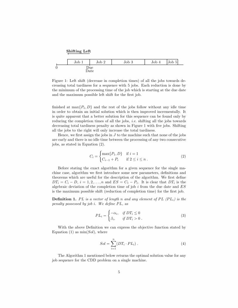
Shifting Left

Figure 1: Left shift (decrease in completion times) of all the jobs towards de-creasing total tardiness for a sequence with 5 jobs. Each reduction is done bythe minimum of the processing time of the job which is starting at the due dateand the maximum possible left shift for the first job.

finished at max{P1, D} and the rest of the jobs follow without any idle timein order to obtain an initial solution which is then improved incrementally. Itis quite apparent that a better solution for this sequence can be found only byreducing the completion times of all the jobs, i.e. shifting all the jobs towardsdecreasing total tardiness penalty as shown in Figure 1 with five jobs. Shiftingall the jobs to the right will only increase the total tardiness.

Hence, we first assign the jobs in J to the machine such that none of the jobsare early and there is no idle time between the processing of any two consecutivejobs, as stated in Equation (2).

Ci =

{

max{P1, D} if i = 1

Ci−1 + Pi if 2 ≤ i ≤ n .(2)

Before stating the exact algorithm for a given sequence for the single ma-chine case, algorithm we first introduce some new parameters, definitions andtheorems which are useful for the description of the algorithm. We first defineDTi = Ci − D, i = 1, 2, . . . , n and ES = C1 − P1. It is clear that DTi is thealgebraic deviation of the completion time of job i from the due date and ESis the maximum possible shift (reduction of completion time) for the first job.

Definition 1. PL is a vector of length n and any element of PL (PLi) is thepenalty possessed by job i. We define PL, as

PLi =

{

−αi, if DTi ≤ 0

βi, if DTi > 0 .(3)

With the above Definition we can express the objective function stated byEquation (1) as min(Sol), where

Sol =

n∑

i=1

(DTi · PLi) . (4)

The Algorithm 1 mentioned below returns the optimal solution value for anyjob sequence for the CDD problem on a single machine.

5

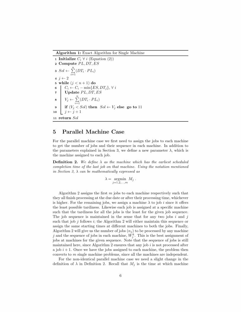
Algorithm 1: Exact Algorithm for Single Machine

1 Initialize Ci ∀ i (Equation (2))2 Compute PL,DT,ES

3 Sol ←n∑

i=1

(DTi · PLi)

4 j ← 25 while (j < n+ 1) do6 Ci ← Ci −min{ES,DTj}, ∀ i7 Update PL,DT,ES

8 Vj ←n∑

i=1

(DTi · PLi)

9 if (Vj < Sol) then Sol← Vj else go to 1110 j ← j + 1

11 return Sol

5 Parallel Machine Case

For the parallel machine case we first need to assign the jobs to each machineto get the number of jobs and their sequence in each machine. In addition tothe parameters explained in Section 3, we define a new parameter λ, which isthe machine assigned to each job.

Definition 2. We define λ as the machine which has the earliest scheduledcompletion time of the last job on that machine. Using the notation mentionedin Section 3, λ can be mathematically expressed as

λ = argminj=1,2,...,m

Mj .

Algorithm 2 assigns the first m jobs to each machine respectively such thatthey all finish processing at the due date or after their processing time, whicheveris higher. For the remaining jobs, we assign a machine λ to job i since it offersthe least possible tardiness. Likewise each job is assigned at a specific machinesuch that the tardiness for all the jobs is the least for the given job sequence.The job sequence is maintained in the sense that for any two jobs i and jsuch that job j follows i; the Algorithm 2 will either maintain this sequence orassign the same starting times at different machines to both the jobs. Finally,Algorithm 2 will give us the number of jobs (nj) to be processed by any machinej and the sequence of jobs in each machine, W k

j . This is the best assignment ofjobs at machines for the given sequence. Note that the sequence of jobs is stillmaintained here, since Algorithm 2 ensures that any job i is not processed aftera job i+ 1. Once we have the jobs assigned to each machine, the problem thenconverts to m single machine problems, since all the machines are independent.

For the non-identical parallel machine case we need a slight change in thedefinition of λ in Definition 2. Recall that Mj is the time at which machine

6

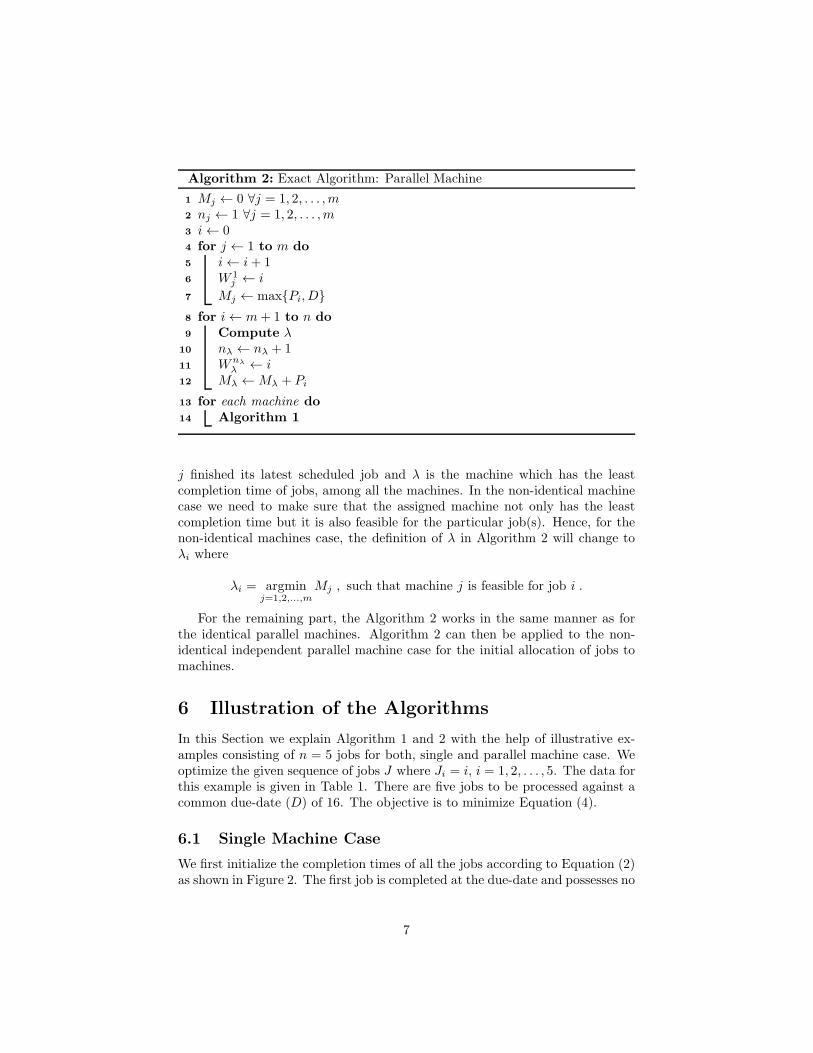
Algorithm 2: Exact Algorithm: Parallel Machine

1 Mj ← 0 ∀j = 1, 2, . . . ,m2 nj ← 1 ∀j = 1, 2, . . . ,m3 i← 04 for j ← 1 to m do

5 i← i+ 16 W 1

j ← i

7 Mj ← max{Pi, D}

8 for i← m+ 1 to n do

9 Compute λ10 nλ ← nλ + 111 Wnλ

λ ← i12 Mλ ←Mλ + Pi

13 for each machine do

14 Algorithm 1

j finished its latest scheduled job and λ is the machine which has the leastcompletion time of jobs, among all the machines. In the non-identical machinecase we need to make sure that the assigned machine not only has the leastcompletion time but it is also feasible for the particular job(s). Hence, for thenon-identical machines case, the definition of λ in Algorithm 2 will change toλi where

λi = argminj=1,2,...,m

Mj , such that machine j is feasible for job i .

For the remaining part, the Algorithm 2 works in the same manner as forthe identical parallel machines. Algorithm 2 can then be applied to the non-identical independent parallel machine case for the initial allocation of jobs tomachines.

6 Illustration of the Algorithms

In this Section we explain Algorithm 1 and 2 with the help of illustrative ex-amples consisting of n = 5 jobs for both, single and parallel machine case. Weoptimize the given sequence of jobs J where Ji = i, i = 1, 2, . . . , 5. The data forthis example is given in Table 1. There are five jobs to be processed against acommon due-date (D) of 16. The objective is to minimize Equation (4).

6.1 Single Machine Case

We first initialize the completion times of all the jobs according to Equation (2)as shown in Figure 2. The first job is completed at the due-date and possesses no

7

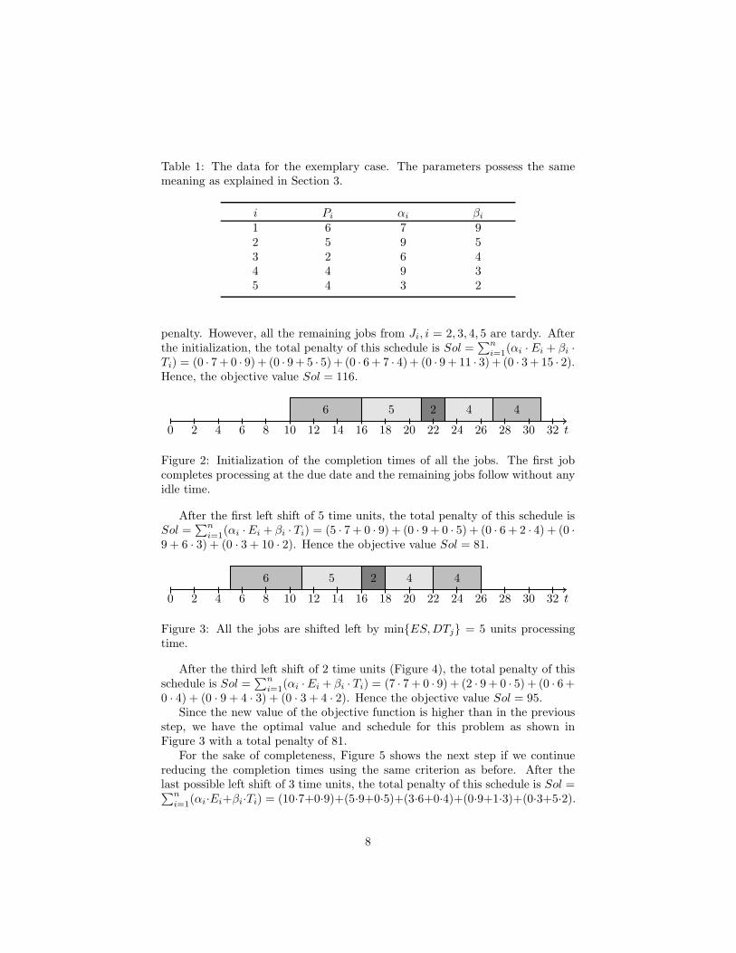
Table 1: The data for the exemplary case. The parameters possess the samemeaning as explained in Section 3.

i Pi αi βi

1 6 7 92 5 9 53 2 6 44 4 9 35 4 3 2

penalty. However, all the remaining jobs from Ji, i = 2, 3, 4, 5 are tardy. Afterthe initialization, the total penalty of this schedule is Sol =

∑n

i=1(αi ·Ei + βi ·

Ti) = (0 · 7+ 0 · 9)+ (0 · 9+ 5 · 5)+ (0 · 6+ 7 · 4)+ (0 · 9+ 11 · 3)+ (0 · 3+ 15 · 2).Hence, the objective value Sol = 116.

6 5 2 4 4

t0 2 4 6 8 10 12 14 16 18 20 22 24 26 28 30 32

Figure 2: Initialization of the completion times of all the jobs. The first jobcompletes processing at the due date and the remaining jobs follow without anyidle time.

After the first left shift of 5 time units, the total penalty of this schedule isSol =

∑n

i=1(αi ·Ei + βi · Ti) = (5 · 7 + 0 · 9) + (0 · 9 + 0 · 5) + (0 · 6 + 2 · 4) + (0 ·

9 + 6 · 3) + (0 · 3 + 10 · 2). Hence the objective value Sol = 81.

6 5 2 4 4

t0 2 4 6 8 10 12 14 16 18 20 22 24 26 28 30 32

Figure 3: All the jobs are shifted left by min{ES,DTj} = 5 units processingtime.

After the third left shift of 2 time units (Figure 4), the total penalty of thisschedule is Sol =

∑n

i=1(αi ·Ei + βi · Ti) = (7 · 7 + 0 · 9) + (2 · 9 + 0 · 5) + (0 · 6+

0 · 4) + (0 · 9 + 4 · 3) + (0 · 3 + 4 · 2). Hence the objective value Sol = 95.Since the new value of the objective function is higher than in the previous

step, we have the optimal value and schedule for this problem as shown inFigure 3 with a total penalty of 81.

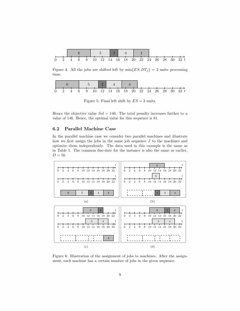
For the sake of completeness, Figure 5 shows the next step if we continuereducing the completion times using the same criterion as before. After thelast possible left shift of 3 time units, the total penalty of this schedule is Sol =∑n

i=1(αi·Ei+βi·Ti) = (10·7+0·9)+(5·9+0·5)+(3·6+0·4)+(0·9+1·3)+(0·3+5·2).

8

6 5 2 4 4

t0 2 4 6 8 10 12 14 16 18 20 22 24 26 28 30 32

Figure 4: All the jobs are shifted left by min{ES,DTj} = 2 units processingtime.

6 5 2 4 4

t0 2 4 6 8 10 12 14 16 18 20 22 24 26 28 30 32

Figure 5: Final left shift by ES = 3 units.

Hence the objective value Sol = 146. The total penalty increases further to avalue of 146. Hence, the optimal value for this sequence is 81.

6.2 Parallel Machine Case

In the parallel machine case we consider two parallel machines and illustratehow we first assign the jobs in the same job sequence J to the machines andoptimize them independently. The data used in this example is the same asin Table 1. The common due-date for the instance is also the same as earlier,D = 16.

0 2 4 6 8 10 12 14 16 18 20 22

t

0 2 4 6 8 10 12 14 16 18 20 22

t

6 5 2 4 4

(a)

0 2 4 6 8 10 12 14 16 18 20 22

t

0 2 4 6 8 10 12 14 16 18 20 22

t

6

5

2 4 4

(b)

0 2 4 6 8 10 12 14 16 18 20 22

t

0 2 4 6 8 10 12 14 16 18 20 22

t

6

5

2

4

44

(c)

0 2 4 6 8 10 12 14 16 18 20 22

t

0 2 4 6 8 10 12 14 16 18 20 22

t

6

5

2

4

4

(d)

Figure 6: Illustration of the assignment of jobs to machines. After the assign-ment, each machine has a certain number of jobs in the given sequence.

9

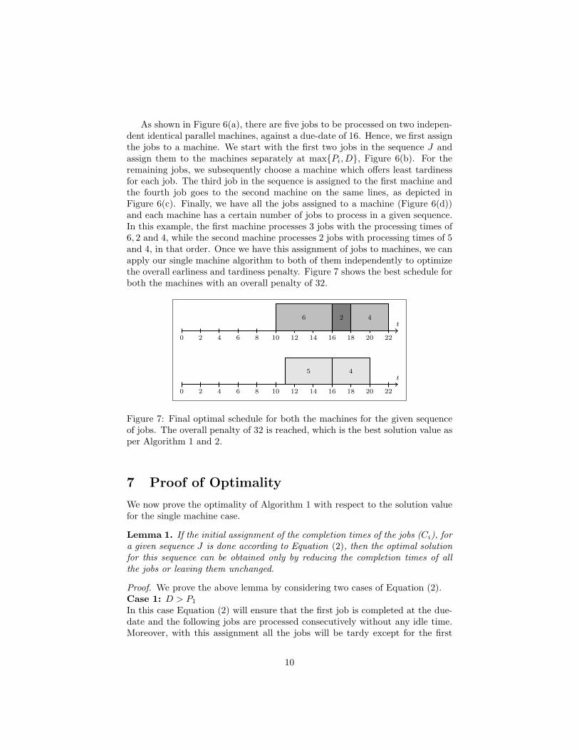
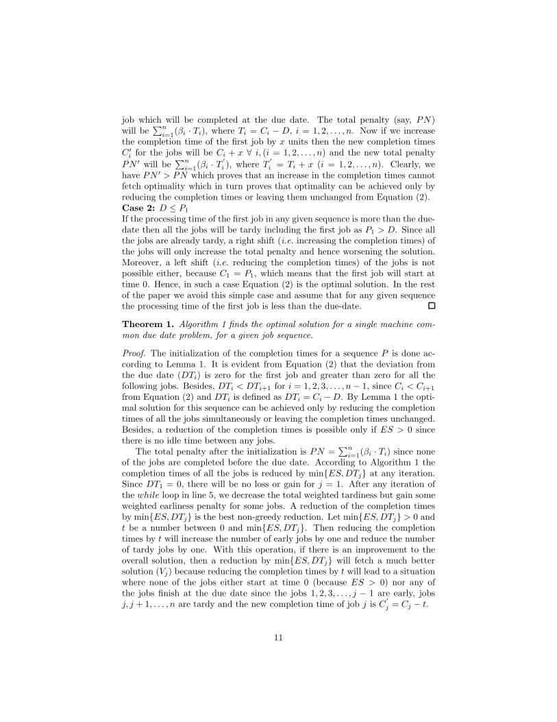
As shown in Figure 6(a), there are five jobs to be processed on two indepen-dent identical parallel machines, against a due-date of 16. Hence, we first assignthe jobs to a machine. We start with the first two jobs in the sequence J andassign them to the machines separately at max{Pi, D}, Figure 6(b). For theremaining jobs, we subsequently choose a machine which offers least tardinessfor each job. The third job in the sequence is assigned to the first machine andthe fourth job goes to the second machine on the same lines, as depicted inFigure 6(c). Finally, we have all the jobs assigned to a machine (Figure 6(d))and each machine has a certain number of jobs to process in a given sequence.In this example, the first machine processes 3 jobs with the processing times of6, 2 and 4, while the second machine processes 2 jobs with processing times of 5and 4, in that order. Once we have this assignment of jobs to machines, we canapply our single machine algorithm to both of them independently to optimizethe overall earliness and tardiness penalty. Figure 7 shows the best schedule forboth the machines with an overall penalty of 32.

0 2 4 6 8 10 12 14 16 18 20 22

t

0 2 4 6 8 10 12 14 16 18 20 22

t

6

5

2

4

4

Figure 7: Final optimal schedule for both the machines for the given sequenceof jobs. The overall penalty of 32 is reached, which is the best solution value asper Algorithm 1 and 2.

7 Proof of Optimality

We now prove the optimality of Algorithm 1 with respect to the solution valuefor the single machine case.

Lemma 1. If the initial assignment of the completion times of the jobs (Ci), fora given sequence J is done according to Equation (2), then the optimal solutionfor this sequence can be obtained only by reducing the completion times of allthe jobs or leaving them unchanged.

Proof. We prove the above lemma by considering two cases of Equation (2).Case 1: D > P1

In this case Equation (2) will ensure that the first job is completed at the due-date and the following jobs are processed consecutively without any idle time.Moreover, with this assignment all the jobs will be tardy except for the first

10

job which will be completed at the due date. The total penalty (say, PN)will be

∑n

i=1(βi · Ti), where Ti = Ci − D, i = 1, 2, . . . , n. Now if we increase

the completion time of the first job by x units then the new completion timesC′

i for the jobs will be Ci + x ∀ i, (i = 1, 2, . . . , n) and the new total penalty

PN ′ will be∑n

i=1(βi · T

′

i ), where T′

i = Ti + x (i = 1, 2, . . . , n). Clearly, wehave PN ′ > PN which proves that an increase in the completion times cannotfetch optimality which in turn proves that optimality can be achieved only byreducing the completion times or leaving them unchanged from Equation (2).Case 2: D ≤ P1

If the processing time of the first job in any given sequence is more than the due-date then all the jobs will be tardy including the first job as P1 > D. Since allthe jobs are already tardy, a right shift (i.e. increasing the completion times) ofthe jobs will only increase the total penalty and hence worsening the solution.Moreover, a left shift (i.e. reducing the completion times) of the jobs is notpossible either, because C1 = P1, which means that the first job will start attime 0. Hence, in such a case Equation (2) is the optimal solution. In the restof the paper we avoid this simple case and assume that for any given sequencethe processing time of the first job is less than the due-date.

Theorem 1. Algorithm 1 finds the optimal solution for a single machine com-mon due date problem, for a given job sequence.

Proof. The initialization of the completion times for a sequence P is done ac-cording to Lemma 1. It is evident from Equation (2) that the deviation fromthe due date (DTi) is zero for the first job and greater than zero for all thefollowing jobs. Besides, DTi < DTi+1 for i = 1, 2, 3, . . . , n− 1, since Ci < Ci+1

from Equation (2) and DTi is defined as DTi = Ci −D. By Lemma 1 the opti-mal solution for this sequence can be achieved only by reducing the completiontimes of all the jobs simultaneously or leaving the completion times unchanged.Besides, a reduction of the completion times is possible only if ES > 0 sincethere is no idle time between any jobs.

The total penalty after the initialization is PN =∑n

i=1(βi · Ti) since none

of the jobs are completed before the due date. According to Algorithm 1 thecompletion times of all the jobs is reduced by min{ES,DTj} at any iteration.Since DT1 = 0, there will be no loss or gain for j = 1. After any iteration ofthe while loop in line 5, we decrease the total weighted tardiness but gain someweighted earliness penalty for some jobs. A reduction of the completion timesby min{ES,DTj} is the best non-greedy reduction. Let min{ES,DTj} > 0 andt be a number between 0 and min{ES,DTj}. Then reducing the completiontimes by t will increase the number of early jobs by one and reduce the numberof tardy jobs by one. With this operation, if there is an improvement to theoverall solution, then a reduction by min{ES,DTj} will fetch a much bettersolution (Vj) because reducing the completion times by t will lead to a situationwhere none of the jobs either start at time 0 (because ES > 0) nor any ofthe jobs finish at the due date since the jobs 1, 2, 3, . . . , j − 1 are early, jobsj, j + 1, . . . , n are tardy and the new completion time of job j is C

′

j = Cj − t.

11

Since after this reductionDTj > 0 andDTj < DTj+1 for j = 1, 2, 3, . . . , n−1,none of the jobs will finish at the due date after a reduction by t units. Moreover,it was proved by Cheng et al. [6] that in an optimal schedule for the restrictivecommon due date, either one of the jobs should start at time 0 or one of thejobs should end at the due date. This case can occur only if we reduce thecompletion times by min{ES,DTj}. If ES < DTj, the first job will start attime 0 and if DTj < ES then one of the jobs will end at the due date. In thenext iterations we continue the reductions as long as we get an improvementin the solution and once the new solution is not better than the previous best,we do not need to check any further and we have our optimal solution. Thiscan be proved by considering the values of the objective function at the indicesof two iterations; j and j + 1. Let Vj and Vj+1 be the value of the objectivefunction at these two indices, then the solution cannot be improved any furtherif Vj+1 > Vj by Lemma 2.

Lemma 2. Once the value of the solution at any iteration j is less than thevalue at iteration j + 1, the solution cannot be improved any further.

Proof. If Vj+1 > Vj , a further left shift of the jobs does not fetch a bettersolution. Note that the objective function has two parts: penalty due to earlinessand penalty due to tardiness. Let us consider the earliness and tardiness of thejobs after the jth iterations are Ej

i and T ji for i = 1, 2, . . . , n. Then we have Vj =

∑n

i=1(αiE

ji + βiT

ji ) and V j+1 =

∑n

i=1(αiE

j+1

i + βiTj+1

i ). Besides, after everyiteration of the while loop in Algorithm 1, the completion times are reduced or inother words the jobs are shifted left. This leads to an increase in the earliness anda decrease in the tardiness of the jobs. Let’s say, the difference in the reductionbetween V j+1 and V j is x. Then we have Ej+1 = Ej + x and Tj+1 = Tj − x.

Since V j+1 > V j , we have:∑n

i=1(αiE

j+1

i + βiTj+1

i ) >∑n

i=1(αiE

ji + βiT

ji ).

By substituting the values of Ej+1 and T j+1 we get,∑j+1

i=1αix >

∑n

i=j+2βix.

Hence, at the (j + 1)th iteration the total penalty due to earliness exceeds thetotal penalty due to tardiness. This proves that for any further reduction therecannot be an improvement in the solution because a decrease in the tardinesspenalty will always be less than the increase in the earliness penalty.

8 Algorithm Run-Time Complexity

In this Section we study and prove the run-time complexity of the Algorithms 1and 2. We calculate the complexities of all the algorithms separately consideringthe worst cases for all. Let T1 and T2 be the run-time complexities of thealgorithms respectively.

Lemma 3. The run-time complexities of both Algorithms 1 and 2 are O(n2),where n is the total number of jobs.

Proof. As for Algorithm 1, the calculations involved in the initialization step andevaluation of PL,DT,ES, Sol are all of O(n) complexity and their evaluation is

12

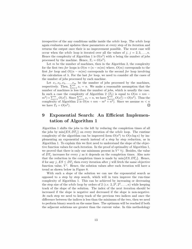
irrespective of the any conditions unlike inside the while loop. The while loopagain evaluates and updates these parameters at every step of its iteration andreturns the output once their is no improvement possible. The worst case willoccur when the while loop is iterated over all the values of j, j = 2, 3, . . . , n.Hence the complexity of Algorithm 1 is O(n2) with n being the number of jobsprocessed by the machine. Hence, T1 = O(n2).

Let m be the number of machines, then in the Algorithm 2, the complexityfor the first two for loops is O(m+(n−m)m) where, O(m) corresponds to thefirst for loop and O((n − m)m) corresponds to the second for loop involvingthe calculation of λ. For the last for loop, we need to consider all the cases ofthe number of jobs processed by each machine.

Let x1, x2, x3, . . . , xm be the number of jobs processed by the machines,respectively. Then,

∑m

i=1xi = n. We make a reasonable assumption that the

number of machines is less than the number of jobs, which is usually the case.In such a case the complexity of Algorithm 2 (T2) is equal to O(m + nm −m2)+

∑m

i=1O(x2

i ). Since∑m

i=1xi = n, we have

∑m

i=1O(x2

i ) = O(n2). Thus thecomplexity of Algorithm 2 is O(m + nm −m2 + n2). Since we assume m < nwe have T2 = O(n2).

9 Exponential Search: An Efficient Implemen-

tation of Algorithm 1

Algorithm 1 shifts the jobs to the left by reducing the completion times of allthe jobs by min{ES,DTj} on every iteration of the while loop. The runtimecomplexity of the algorithm can be improved form O(n2) to O(n logn) by im-plementing an exponential search instead of a step by step reduction, as inAlgorithm 1. To explain this we first need to understand the slope of the objec-tive function values for each iteration. In the proof of optimality of Algorithm 1,we proved that there is only one minimum present in V j ∀j. Besides, the valueof DTj increases for every j as it depends on the completion times. Also notethat the reduction in the completion times is made by min{ES,DTj}. Hence,if for any j, ES ≤ DTj then every iteration after j will fetch the same objectivefunction value, V j . Hence, the solution values after each iteration will have atrend as shown below in Figure 8.

With such a slope of the solution we can use the exponential search asopposed to a step by step search, which will in turn improve the run-timecomplexity of Algorithm 1. This can be achieved by increasing or decreasingthe step size of the while loop by orders of 2 (i.e. 2, 22, 23, . . . , n) while keepingtrack of the slope of the solution. The index of the next iteration should beincreased if the slope is negative and decreased if the slope is non-negative.At each step we need to keep track of the previous two indices and once thedifference between the indices is less than the minimum of the two, then we needto perform binary search on the same lines. The optimum will be reached if boththe adjacent solutions are greater than the current value. In this methodology

13

j0 1 ES ≤ DTjn

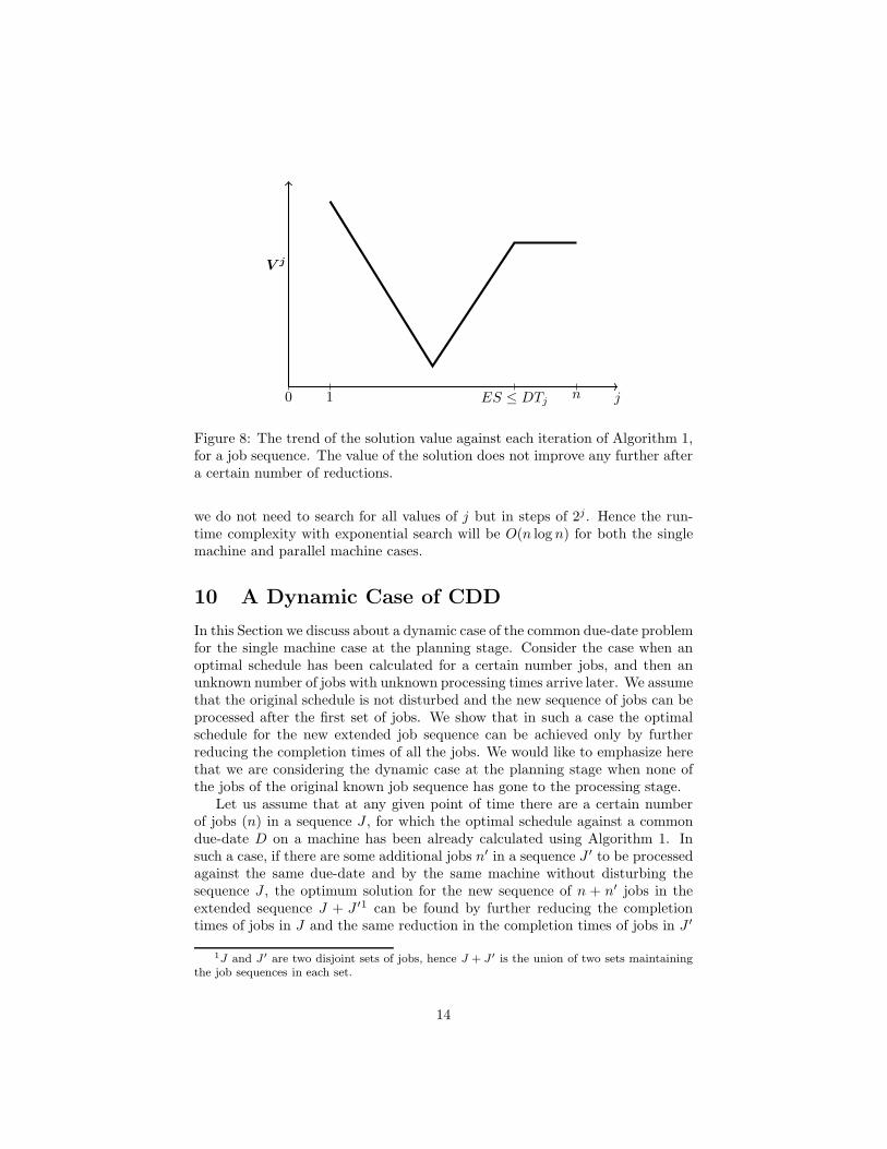
Vj

Figure 8: The trend of the solution value against each iteration of Algorithm 1,for a job sequence. The value of the solution does not improve any further aftera certain number of reductions.

we do not need to search for all values of j but in steps of 2j. Hence the run-time complexity with exponential search will be O(n log n) for both the singlemachine and parallel machine cases.

10 A Dynamic Case of CDD

In this Section we discuss about a dynamic case of the common due-date problemfor the single machine case at the planning stage. Consider the case when anoptimal schedule has been calculated for a certain number jobs, and then anunknown number of jobs with unknown processing times arrive later. We assumethat the original schedule is not disturbed and the new sequence of jobs can beprocessed after the first set of jobs. We show that in such a case the optimalschedule for the new extended job sequence can be achieved only by furtherreducing the completion times of all the jobs. We would like to emphasize herethat we are considering the dynamic case at the planning stage when none ofthe jobs of the original known job sequence has gone to the processing stage.

Let us assume that at any given point of time there are a certain numberof jobs (n) in a sequence J , for which the optimal schedule against a commondue-date D on a machine has been already calculated using Algorithm 1. Insuch a case, if there are some additional jobs n′ in a sequence J ′ to be processedagainst the same due-date and by the same machine without disturbing thesequence J , the optimum solution for the new sequence of n + n′ jobs in theextended sequence J + J ′1 can be found by further reducing the completiontimes of jobs in J and the same reduction in the completion times of jobs in J ′

1J and J ′ are two disjoint sets of jobs, hence J + J ′ is the union of two sets maintainingthe job sequences in each set.

14

using Algorithm 1. We prove it using Lemma 4.

Lemma 4. Let, Ci (i = 1, 2, . . . , n) be the optimal completion times of jobs insequence J and C′

j (j = 1, 2, . . . , n, n+ 1, . . . , n+ n′ − 1, n+ n′) be the optimalcompletion times of jobs in the extended job sequence J + J ′ with n + n′ jobs.Then,

i) ∃ γ ≥ 0 s.t. Ci − C′i = γ for i = 1, 2, . . . , n

ii) C′k = Cn − γ +

∑k

τ=n+1Pτ , (k = n+ 1, n+ 2, . . . , n+ n′) .

Proof. Let SolJ denote the optimal solution for the job sequence J . This optimalvalue for sequence J is calculated using Algorithm 1 which is optimal accordingto Theorem 1. In the optimal solution let the individual penalties for earlinessand tardiness be Ei and Ti, respectively, hence

SolJ =

n∑

i=1

(αiEi + βiTi) . (5)

Clearly, the value of SolJ cannot be improved by either reducing the completiontimes any further as explained in Theorem 1. Now, processing an additional jobsequence J ′ starting from Cn (the completion time of the last job in J) meansthat for the new extended sequence J+J ′ the tardiness penalty increases furtherby some value, say PTJ′ . Besides, the due date remains the same, the sequenceJ is not disturbed and all the jobs in the sequence J ′ are tardy. Hence the newsolution value (say VJ+J′) for the new sequence J + J ′ will be

VJ+J′ = SolJ + PTJ′ . (6)

For this new sequence we do not need to increase the completion times sinceit will only increase the tardiness penalty. This can be proved by contradiction.Let x be the increase in the completion times of all the jobs in J + J ′ withx > 0. The earliness and tardiness for the jobs in J become Ei − x and Ti + x,respectively and the new total penalty (VJ ) for the job sequence J becomes

VJ =n∑

i=1

(αi · (Ei − x) + βi · (Ti + x))

=n∑

i=1

(αi ·Ei + βi · Ti) +n∑

i=1

(βi − αi) · x .(7)

Equation (5) yields

VJ = SolJ +

n∑

i=1

(βi − αi) · x . (8)

Since SolJ is optimal SolJ ≤ VJ , we have

n∑

i=1

(βi − αi) · x ≥ 0 . (9)

15

Besides, the total tardiness penalty for the sequence J ′ will further increaseby the same quantity, say δ, δ ≥ 0. With this shift, the new overall solutionvalue V ′

J+J′ will be

V ′J+J′ = VJ + PTJ′ + δ . (10)

Substituting VJ from Equation (8) we have

V ′J+J′ = SolJ +

n∑

i=1

(βi − αi) · x+ PTJ′ + δ . (11)

Using Equation (6) gives

V ′J+J′ = VJ+J′ +

n∑

i=1

(βi − αi) · x+ δ . (12)

Using Equation (9) and δ ≥ 0 we have

V ′J+J′ ≥ VJ+J′ . (13)

This shows that only a reduction in the completion times of all the jobs canimprove the solution. Thus, there exists a γ, γ ≥ 0 by which the completiontimes are reduced to achieve the optimal solution for the new job sequenceJ + J ′. Clearly, Ci −C′

i = γ for i = 1, 2, . . . , n and C′k = Cn − γ +

∑k

τ=n+1Pτ ,

(k = n+ 1, n+ 2, . . . , n+ n′) since all the jobs are processed one after anotherwithout any idle time.

11 Results

In this Section we present our results for the single and parallel machine cases.We used our exact algorithms with simulated annealing for finding the best jobsequence. All the algorithms were implemented on MATLAB R© and run on amachine with a 1.73 GHz processor and 2 GB RAM. We present our results forthe benchmark instances provided by Biskup and Feldmann in [4] for both thesingle and parallel machine cases. For brevity, we call our approach as APSAand the benchmark results as BR.

We use a modified Simulated Annealing algorithm to generate job sequencesand Algorithm 1 to optimize each sequence to its minimum penalty. Our ex-periments show that an ensemble size of 4+n/10 and the maximum number ofiterations as 500 · n, where n is the number of jobs, work best for the providedbenchmark instances. The runtime for all the results is the time after whichthe solutions mentioned in Table 2 and 3 are obtained. The initial tempera-ture is kept as twice the standard deviation of the energy at infinite tempera-ture: σET=∞

=√

〈E2〉T=∞ − 〈E〉2T=∞. We estimate this quantity by randomlysampling the configuration space [18]. An exponential schedule for cooling is

16

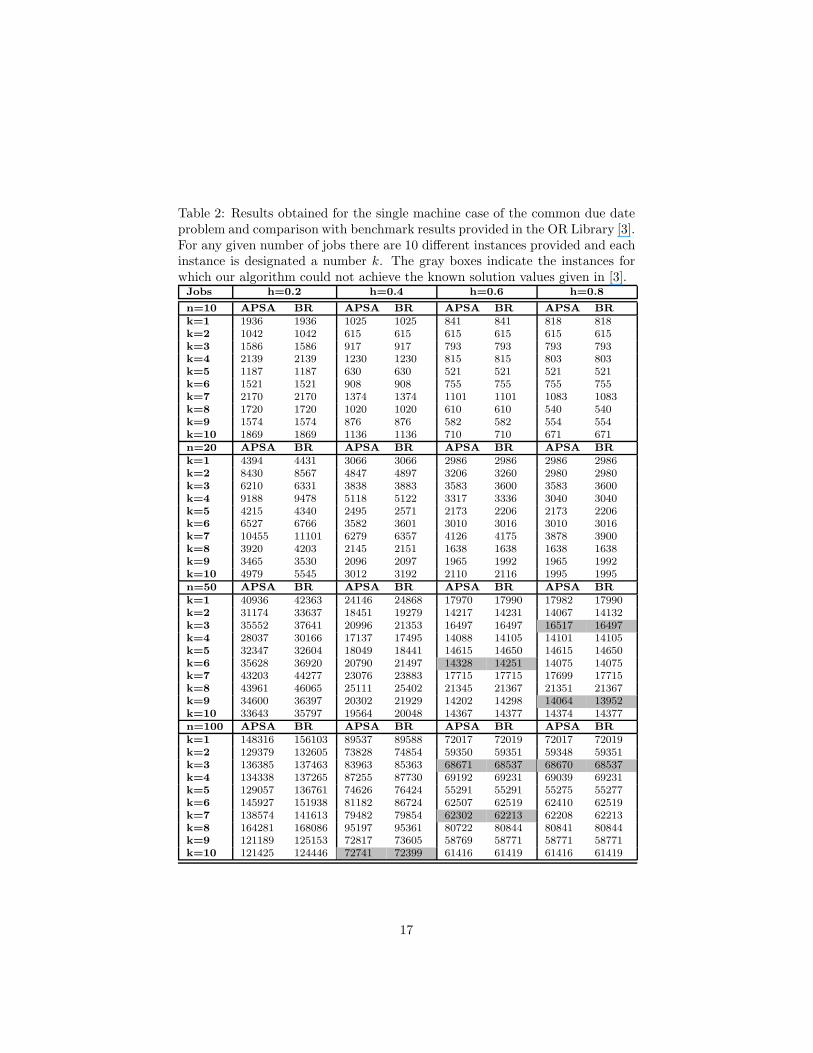
Table 2: Results obtained for the single machine case of the common due dateproblem and comparison with benchmark results provided in the OR Library [3].For any given number of jobs there are 10 different instances provided and eachinstance is designated a number k. The gray boxes indicate the instances forwhich our algorithm could not achieve the known solution values given in [3].Jobs h=0.2 h=0.4 h=0.6 h=0.8

n=10 APSA BR APSA BR APSA BR APSA BRk=1 1936 1936 1025 1025 841 841 818 818k=2 1042 1042 615 615 615 615 615 615k=3 1586 1586 917 917 793 793 793 793k=4 2139 2139 1230 1230 815 815 803 803k=5 1187 1187 630 630 521 521 521 521k=6 1521 1521 908 908 755 755 755 755k=7 2170 2170 1374 1374 1101 1101 1083 1083k=8 1720 1720 1020 1020 610 610 540 540k=9 1574 1574 876 876 582 582 554 554k=10 1869 1869 1136 1136 710 710 671 671n=20 APSA BR APSA BR APSA BR APSA BRk=1 4394 4431 3066 3066 2986 2986 2986 2986k=2 8430 8567 4847 4897 3206 3260 2980 2980k=3 6210 6331 3838 3883 3583 3600 3583 3600k=4 9188 9478 5118 5122 3317 3336 3040 3040k=5 4215 4340 2495 2571 2173 2206 2173 2206k=6 6527 6766 3582 3601 3010 3016 3010 3016k=7 10455 11101 6279 6357 4126 4175 3878 3900k=8 3920 4203 2145 2151 1638 1638 1638 1638k=9 3465 3530 2096 2097 1965 1992 1965 1992k=10 4979 5545 3012 3192 2110 2116 1995 1995n=50 APSA BR APSA BR APSA BR APSA BRk=1 40936 42363 24146 24868 17970 17990 17982 17990k=2 31174 33637 18451 19279 14217 14231 14067 14132k=3 35552 37641 20996 21353 16497 16497 16517 16497k=4 28037 30166 17137 17495 14088 14105 14101 14105k=5 32347 32604 18049 18441 14615 14650 14615 14650k=6 35628 36920 20790 21497 14328 14251 14075 14075k=7 43203 44277 23076 23883 17715 17715 17699 17715k=8 43961 46065 25111 25402 21345 21367 21351 21367k=9 34600 36397 20302 21929 14202 14298 14064 13952k=10 33643 35797 19564 20048 14367 14377 14374 14377n=100 APSA BR APSA BR APSA BR APSA BRk=1 148316 156103 89537 89588 72017 72019 72017 72019k=2 129379 132605 73828 74854 59350 59351 59348 59351k=3 136385 137463 83963 85363 68671 68537 68670 68537k=4 134338 137265 87255 87730 69192 69231 69039 69231k=5 129057 136761 74626 76424 55291 55291 55275 55277k=6 145927 151938 81182 86724 62507 62519 62410 62519k=7 138574 141613 79482 79854 62302 62213 62208 62213k=8 164281 168086 95197 95361 80722 80844 80841 80844k=9 121189 125153 72817 73605 58769 58771 58771 58771k=10 121425 124446 72741 72399 61416 61419 61416 61419

17

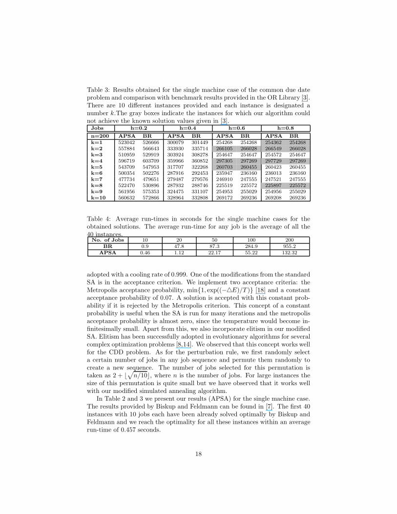
Table 3: Results obtained for the single machine case of the common due dateproblem and comparison with benchmark results provided in the OR Library [3].There are 10 different instances provided and each instance is designated anumber k.The gray boxes indicate the instances for which our algorithm couldnot achieve the known solution values given in [3].Jobs h=0.2 h=0.4 h=0.6 h=0.8

n=200 APSA BR APSA BR APSA BR APSA BRk=1 523042 526666 300079 301449 254268 254268 254362 254268k=2 557884 566643 333930 335714 266105 266028 266549 266028k=3 510959 529919 303924 308278 254647 254647 254572 254647k=4 596719 603709 359966 360852 297305 297269 297729 297269k=5 543709 547953 317707 322268 260703 260455 260423 260455k=6 500354 502276 287916 292453 235947 236160 236013 236160k=7 477734 479651 279487 279576 246910 247555 247521 247555k=8 522470 530896 287932 288746 225519 225572 225897 225572k=9 561956 575353 324475 331107 254953 255029 254956 255029k=10 560632 572866 328964 332808 269172 269236 269208 269236

Table 4: Average run-times in seconds for the single machine cases for theobtained solutions. The average run-time for any job is the average of all the40 instances.No. of Jobs 10 20 50 100 200

BR 0.9 47.8 87.3 284.9 955.2APSA 0.46 1.12 22.17 55.22 132.32

adopted with a cooling rate of 0.999. One of the modifications from the standardSA is in the acceptance criterion. We implement two acceptance criteria: theMetropolis acceptance probability, min{1, exp((−△E)/T )} [18] and a constantacceptance probability of 0.07. A solution is accepted with this constant prob-ability if it is rejected by the Metropolis criterion. This concept of a constantprobability is useful when the SA is run for many iterations and the metropolisacceptance probability is almost zero, since the temperature would become in-finitesimally small. Apart from this, we also incorporate elitism in our modifiedSA. Elitism has been successfully adopted in evolutionary algorithms for severalcomplex optimization problems [8,14]. We observed that this concept works wellfor the CDD problem. As for the perturbation rule, we first randomly selecta certain number of jobs in any job sequence and permute them randomly tocreate a new sequence. The number of jobs selected for this permutation istaken as 2 + ⌊

√

n/10⌋, where n is the number of jobs. For large instances thesize of this permutation is quite small but we have observed that it works wellwith our modified simulated annealing algorithm.

In Table 2 and 3 we present our results (APSA) for the single machine case.The results provided by Biskup and Feldmann can be found in [7]. The first 40instances with 10 jobs each have been already solved optimally by Biskup andFeldmann and we reach the optimality for all these instances within an averagerun-time of 0.457 seconds.

18

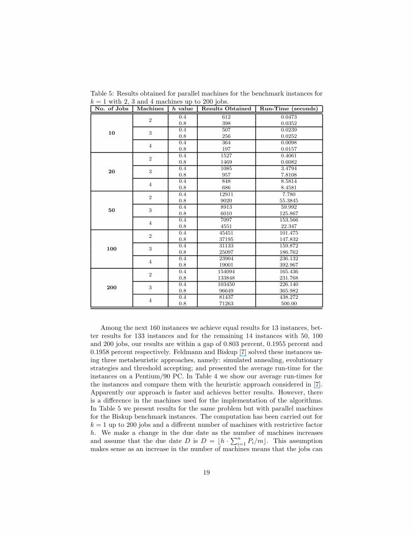
Table 5: Results obtained for parallel machines for the benchmark instances fork = 1 with 2, 3 and 4 machines up to 200 jobs.No. of Jobs Machines h value Results Obtained Run-Time (seconds)

10

20.4 612 0.04730.8 398 0.0352

30.4 507 0.02390.8 256 0.0252

40.4 364 0.00980.8 197 0.0157

20

20.4 1527 0.40610.8 1469 0.6082

30.4 1085 3.47940.8 957 7.8108

40.4 848 8.58140.8 686 8.4581

50

20.4 12911 7.7800.8 9020 55.3845

30.4 8913 59.9920.8 6010 125.867

40.4 7097 153.5660.8 4551 22.347

100

20.4 45451 101.4750.8 37195 147.832

30.4 31133 159.8720.8 25097 186.762

40.4 23904 236.1320.8 19001 392.967

200

20.4 154094 165.4360.8 133848 231.768

30.4 103450 226.1400.8 96649 365.982

40.4 81437 438.2720.8 71263 500.00

Among the next 160 instances we achieve equal results for 13 instances, bet-ter results for 133 instances and for the remaining 14 instances with 50, 100and 200 jobs, our results are within a gap of 0.803 percent, 0.1955 percent and0.1958 percent respectively. Feldmann and Biskup [7] solved these instances us-ing three metaheuristic approaches, namely: simulated annealing, evolutionarystrategies and threshold accepting; and presented the average run-time for theinstances on a Pentium/90 PC. In Table 4 we show our average run-times forthe instances and compare them with the heuristic approach considered in [7].Apparently our approach is faster and achieves better results. However, thereis a difference in the machines used for the implementation of the algorithms.In Table 5 we present results for the same problem but with parallel machinesfor the Biskup benchmark instances. The computation has been carried out fork = 1 up to 200 jobs and a different number of machines with restrictive factorh. We make a change in the due date as the number of machines increasesand assume that the due date D is D = ⌊h ·

∑n

i=1Pi/m⌋. This assumption

makes sense as an increase in the number of machines means that the jobs can

19

be completed much faster and reducing the due-date will test the whole setupfor more competitive scenarios. We implemented Algorithm 2 with six differentcombinations of the number of machines and the restrictive factor. Since theseinstances have not been solved for the parallel machines, we are presenting theupper bounds achieved for these instances using Algorithm 2 and the modifiedsimulated annealing.

12 Conclusion and Future Direction

In this paper we present two novel exact polynomial algorithms for the commondue-date problem to optimize any given job sequence. We prove the optimalityfor the single machine case and the run-time complexity of the algorithms. Weimplemented our algorithms over the benchmark instances provided by Biskupand Feldmann [4] and the results obtained by using our algorithms are superiorto the benchmark results in quality. We discuss how our approach can be usedfor non-identical parallel machines and present results for the parallel machinecase for the same instances. Furthermore, we also discuss the efficiency of ouralgorithm for a special dynamic case of CDD at the planning stage.

Acknowledgement

The research project was promoted and funded by the European Union andthe Free State of Saxony, Germany. The authors take the responsibility for thecontent of this chapter.

References

[1] Awasthi, A., Lassig, J., Kramer, O.: Common due-date problem: Exactpolynomial algorithms for a given job sequence. In: 15th InternationalSymposium on Symbolic and Numeric Algorithms for Scientific Computing(SYNASC 2013), pp. 260–266 (2013)

[2] Banisadr, A.H., Zandieh, M., Mahdavi, I.: A hybrid imperialist competi-tive algorithm for single-machine scheduling problem with linear earlinessand quadratic tardiness penalties. The International Journal of AdvancedManufacturing Technology 65(5–8), 981–989 (2013)

[3] Beasley, J.E.: OR-library: Distributing test problems by electronic mail.Journal of the Operational Research Society 41(11), 1069–1072 (1990)

[4] Biskup, D., Feldmann, M.: Benchmarks for scheduling on a single ma-chine against restrictive and unrestrictive common due dates. Computers& Operations Research 28(8), 787 – 801 (2001)

[5] Cheng, T.C.E.: Optimal due-date assignment and sequencing in a singlemachine shop. Applied Mathematics Letters 2(1), 21–24 (1989)

20

[6] Cheng, T.C.E., Kahlbacher, H.G.: A proof for the longest-job-first policyin one-machine scheduling. Naval Research Logistics (NRL) 38(5), 715–720(1991)

[7] Feldmann, M., Biskup, D.: Single-machine scheduling for minimizing ear-liness and tardiness penalties by meta-heuristic approaches. Computers &Industrial Engineering 44(2), 307–323 (2003)

[8] Gen, M., Tsujimura, Y., Kubota, E.: Solving job-shop scheduling problemsby genetic algorithm. In: IEEE International Conference on Systems, Man,and Cybernetics, 1994. Humans, Information and Technology., vol. 2, pp.1577–1582 (1994)

[9] Graham, R.L., Lawler, E.L., Lenstra, J.K., Rinnooy Kan, A.H.G.: Opti-mization and approximation in deterministic sequencing and scheduling: asurvey. In: Discrete Optimization II Proceedings of the Advanced ResearchInstitute on Discrete Optimization and Systems Applications of the Sys-tems Science Panel of NATO and of the Discrete Optimization Symposiumco-sponsored by IBM Canada and SIAM Banff, Aha. and Vancouver, vol. 5,pp. 287 – 326. Elsevier (1979)

[10] Hall, N.G., Kubiak, W., Sethi, S.P.: Earliness–tardiness scheduling prob-lems, ii: deviation of completion times about a restrictive common duedate. Operations Research 39(5), 847–856 (1991)

[11] Hoogeveen, J.A., Van de Velde, S.L.: Scheduling around a small commondue date. European Journal of Operational Research 55(2), 237–242 (1991)

[12] James, R.J.W.: Using tabu search to solve the common due dateearly/tardy machine scheduling problem. Computers & Operations Re-search 24(3), 199–208 (1997)

[13] Kanet, J.J.: Minimizing the average deviation of job completion timesabout a common due date. Naval Research Logistics Quarterly 28(4), 643–651 (1981)

[14] Kim, J.L.: Genetic algorithm stopping criteria for optimization of con-struction resource scheduling problems. Construction Management andEconomics 31(1), 3–19 (2013)

[15] Panwalkar, S.S., Smith, M.L., Seidmann, A.: Common due date assign-ment to minimize total penalty for the one machine scheduling problem.Operations Research 30(2), 391–399 (1982)

[16] Rebai, M., Kacem, I., Adjallah, K.H.: Earliness-tardiness minimization ona single machine to schedule preventive maintenance tasks: metaheuristicand exact methods. Journal of Intelligent Manufacturing 23(4), 1207–1224(2012)

21

[17] Ronconi, D.P., Kawamura, M.S.: The single machine earliness and tardi-ness scheduling problem: lower bounds and a branch-and-bound algorithm.Computational & Applied Mathematics 29, 107 – 124 (2010)

[18] Salamon, P., Sibani, P., Frost, R.: Facts, Conjectures, and Improvementsfor Simulated Annealing. Society for Industrial and Applied Mathematics(2002). DOI 10.1137/1.9780898718300

[19] Seidmann, A., Panwalkar, S.S., Smith, M.L.: Optimal assignment of due-dates for a single processor scheduling problem. The International JournalOf Production Research 19(4), 393–399 (1981)

[20] Toksari, M.D., Guner, E.: The common due-date early/tardy schedulingproblem on a parallel machine under the effects of time-dependent learningand linear and nonlinear deterioration. Expert Systems with Applications37(1), 92–112 (2010)

[21] Yang, S.J., Lee, H.T., Guo, J.Y.: Multiple common due dates assignmentand scheduling problems with resource allocation and general position-dependent deterioration effect. The International Journal of AdvancedManufacturing Technology 67(1-4), 181–188 (2013)

22