a new noble gas paleoclimate record in texas — basic assumptions revisited

tters 257 (2007) 170–187www.elsevier.com/locate/epsl

Earth and Planetary Science Le

A new noble gas paleoclimate record inTexas — Basic assumptions revisited

Maria Clara Castro a,⁎, Chris Michael Hall a, Delphine Patriarche b,1,Patrick Goblet c, Brian Robert Ellis a,2

a University of Michigan, Department of Geological Sciences, 2534 C. C. Little Building, Ann Arbor, MI 48109 - 1005, United Statesb Commissariat à l'Energie Atomique, 91680 Bruyères-le-Châtel, France

c Ecole des Mines de Paris, Centre de Géosciences, 77305 Fontainebleau, France

Received 25 July 2006; received in revised form 19 February 2007; accepted 19 February 2007

Available onlin

Editor: R.D. van der Hilst

e 27 February 2007

Abstract

A generally accepted basic principle in relation to the use of the noble gas thermometer in groundwater flow systems is that high-frequency noble gas climatic signals are lost due to the effect of dispersion. This loss of signal, combinedwith 14C dating issues, makes itonly suited to identify major climatic events such as the Last Glacial Maximum (LGM). Consequently, the identification of significantnoble gas temperature (NGT) cooling (≥5 °C) with respect to present time has systematically been associated with the occurrence of theLGM even when reasonable water age controls were unavailable. It has also become apparent at a number of studied sites that modernNGTs estimated through standardmodels [M. Stute, P. Schlosser, Principles and applications of the noble gas paleothermometer, in: P.K.Swart, K.C. Lohmann, J.A. McKenzie, S. Savin, (Eds), Climate change in continental isotopic records, Geophysical monograph 78,AGU (1993) 89-100.; W. Aeschbach-Hertig, F. Peeters, U. Beyerle, R. Kipfer, Paleotemperature reconstruction from noble gases inground water taking into account equilibration with entrapped air, Nature 405(6790) (2000) 1040-1044.] are unable to reproduce groundtemperatures at the interface with the unsaturated zone, a basic requirement for proper paleoclimate reconstruction through noble gases.Instead, a systematic bias to low NGTs in recharge areas is observed. The Carrizo aquifer, in which the LGM was previously identified[M. Stute, P. Schlosser, J.F. Clark, W.S. Broecker, Paleotemperatures in the Southwestern United States derived from noble gases inground water, Science 256(5059) (1992) 1000-1001.] and which presents an NGT bias of over 4 °C, is an ideal setting to analyze andrevise basic principles and assumptions in relation with the use of the noble gas thermometer.

Here, we present a new noble gas data set (49 measurements) collected at 20 different locations in the Carrizo aquifer. This newdata set together with previously published data (20 measurements) was used to calibrate a 3-D groundwater flow and 4He transportmodel in which simulations of groundwater age were subsequently carried out. These account for mixing processes due toadvection, dispersion, diffusion, and cross-formational flow.

We first show that samples previously attributed to the LGM belong in fact to the middle Holocene. Through a step-by-stepapproach we then proceed to carry out a comparative analysis of both the impact of dispersion on high frequency climatic signalsand assumptions underlying competing NGT models. Our combined analysis indicates that groundwater flow systems, at least

⁎ Corresponding author. Tel.: +1 734 615 3812; fax: +1 734 763 4690.E-mail addresses: [email protected] (M.C. Castro), [email protected] (C.M. Hall), [email protected] (D. Patriarche),

[email protected] (P. Goblet), [email protected] (B.R. Ellis).1 Now at Gaz de France, 361, avenue du President Wilson, 93211 La Plaine Saint Denis, France.2 Now at Princeton University, Department of Civil and Environmental Engineering, E-223 E-Quad, Princeton, NJ 08540.

0012-821X/$ - see front matter © 2007 Elsevier B.V. All rights reserved.doi:10.1016/j.epsl.2007.02.030

mailto:[email protected]





http://dx.doi.org/10.1016/j.epsl.2007.02.030

171M.C. Castro et al. / Earth and Planetary Science Letters 257 (2007) 170–187

those with similar characteristics to that of the Carrizo, do have the ability to preserve short term (100–200 yrs) climaticfluctuations archived by noble gases. It also shows that abrupt climate shifts during the mid-late Holocene which are associatedwith significant NGT changes (≥5 °C) do not reflect equally important changes in the mean annual atmospheric temperature(MAAT). Instead, these reflect the combined effect of atmospheric temperature changes, seasonality of recharge and, above all,significant variations of the water table depth which result from shifts between humid and arid regimes. Together with NGTs, ourexcess air record plays a critical role in identifying such abrupt climate changes. Specifically, the Carrizo combined data setindicates an abrupt shift from a cool, humid regime to a warmer, arid one at ∼ 1 kyrs BP. A major Holocene (∼ 6 kyrs BP) NGTchange of 7.7 °C with respect to present now identified is mostly the result of a dramatic water table drop which occurred duringthe ∼ 1 kyrs BP transition period. Current NGTs in the Carrizo recharge area do not appear to be recording atmospheric changes.Rather, these are recording ground conditions reflecting mostly the impact of heat flow in the area. We also show that observedsystematic offsets in NGT recharge areas can be reconciled through NGT estimation models which account for a noble gas partialpressure increase in the unsaturated zone, potentially due to O2 depletion.© 2007 Elsevier B.V. All rights reserved.

Keywords: noble gas temperatures; groundwater flow modeling; simulation of groundwater ages; high-frequency climatic signals; dispersion

1. Introduction

Because noble gases (Ne, Ar, Kr, and Xe) are conserv-ative tracers and their concentrations in the recharge areasof groundwater systems are typically considered to besimply a function of temperature, altitude, excess air, andsalinity, noble gas temperatures (NGTs) are commonlyregarded as a potentially robust indicator of past climate[1–3].

Meaningful paleoclimatic reconstructions throughNGTs, however, require a number of conditions andbasic assumptions to be fulfilled (e.g., [4]). The mostimmediate one is availability of reasonably accurate waterage information. Correspondence between NGTs andgroundwater age has been typically done based on 14Cages, a dating tool that remains problematic in manygroundwater flow systems (e.g., [5–7]). Another generallyaccepted basic principle is that high-frequency noble gasclimatic signals are lost or severely diminished in mostgroundwater systems due to the effect of dispersion [1,2].Because of the combined effect of high-frequency signalloss and 14C dating issues, it was concluded that the noblegas thermometer cannot be used to identify short-termclimatic fluctuations, but instead, is only suited to identifymajor climatic events such as the Last Glacial Maximum(LGM) [3]. Consequently, the identification of importantcooling (≥5 °C) with respect to present time throughNGTs has systematically been associated with theoccurrence of the LGM. In some cases, such associationshave been made despite the lack of reasonable water agecontrols (e.g., [8,5]).

Another basic requirement for the application of thenoble gas thermometer is that noble gases should closelyrecord themean annual temperature at the water table, i.e.,the ground temperature at the interface with the saturatedzone [3,1]. Until recently, with the exception of estimated

water table NGTs systematically lower (∼ 2.2 °C) withrespect to soil temperature observed in Bocholt, Germany[4], no other NGT biases in recharge areas have beenreported in the literature. Such depressed NGTs wereattributed to the effect of vegetation, presumably due todepressed ground temperature. A recent and detailedstudy in southern Michigan [9,10], however, also foundthat estimated water table NGTs were systematicallydepressed with respect to ground temperature. These wereestimated using the two most common and widelyaccepted models, i.e., the unfractionated air (UA) modelas developed by Stute and Schlosser [1], and thecontinuous equilibration (CE) model [11]. As demon-strated by Hall et al. [10], both models display differing(2.5–4 °C) but systematically depressed NGTs comparedto ground temperature at the interface with thewater table.A closer look at previously published NGT data indicatesthat at least in some cases, equally important biases areobserved elsewhere. For example, temperature measure-ments in recharge waters of the Carrizo aquifer,southwestern Texas (e.g., [12]) indicate that previouslyreported [8,13] NGTs in this area are also depressed withrespect to ground temperature by ∼ 4.2 °C. Thissignificant bias to low NGTs in recharge areas in verydistinct climatic regions, i.e., temperate (Germany,southeastern Michigan) versus semi-arid (southwestTexas) is a clear indication that assumptions of both theUA and CE models do not adequately describe all themechanisms controlling noble gas concentrations (e.g.,increased noble gas partial pressure, modification of gassolubility due to reduced soil humidity, etc.) and thus,NGTs in these areas (e.g., [14,10]).

Issues of groundwater dating and preservation or loss ofhigh versus low frequency climatic signals in groundwatersystems are intrinsically related to the specific character-istics of each individual system. As already pointed out by

172 M.C. Castro et al. / Earth and Planetary Science Letters 257 (2007) 170–187

Favreau et al. [15], in order to correctly interpret NGTrecords as well as to improve our understanding of themechanisms controlling the original input of atmosphericnoble gas concentrations, a reasonable knowledge of thedynamics of the groundwater system in question both inthe confined and unconfined areas is required. Improvedand increased density data sets will also play a critical rolein reaching such goals.

Groundwater flow, heat transfer, and helium transportin the Carrizo aquifer and surrounding formations havebeen extensively studied in recent years (e.g., [12,16–18]). Such studies were carried out with the aide of 1-, 2-,and 3-D numerical and geostatistical models throughincorporation of large primary data sets. Issues ofgroundwater age estimation in this particular systemhave also been analyzed [7]. This background worktogether with a new noble gas data set renders the Carrizoaquifer an ideal candidate to further analyze and deepenour understanding of the information archived by thenoble gas thermometer in groundwater flow systems.

Here, through a combination of 3-D simulations ofgroundwater flow, 4He transport, and groundwater agesas well as a comparative analysis of both the impact ofdispersion on high-frequency climatic signals andassumptions underlying competing NGT models, weaddress some basic issues in relation to the use of thenoble gas thermometer in groundwater flow systems.Our analysis is based on the combined previouslypublished [8,19] and new (this study) data sets.

Overall this work attempts to clarify a number ofissues relating to the use of the noble gas thermometer ingroundwater flow systems and to address apparentinconsistencies between NGTs and ground temperaturewhich, at present, widely used and sophisticated NGTsmodels (e.g., UA, CE) remain unable to resolve.

2. Geological and hydrogeological background

The Carrizo aquifer, a major groundwater flowsystem in Texas, is part of a thick regressive sequenceof terrigenous clastics that formed within fluvial, deltaicand marine depositional systems in the Rio GrandeEmbayment area of South Texas on the northwesternmargin of the Gulf Coast Basin (Fig. 1a).

In the study area (Fig. 1b) the Carrizo aquifer is aconfined, massive sandstone lying unconformably on theWilcox formation (Fig. 1c; [20,21]). Downdip, theCarrizo contains an increasing amount of shales andmudstones [22,23]. The thickness of the Carrizo is highlyvariable, ranging from 50 m in the southern part ofMcMullen County to about 350 m in the northern part ofLive Oak County. The underlying lower-Wilcox, the

oldest formation of Tertiary age, contains thick mudstoneand clay layers. The Recklaw formation, a confining layerprimarily composed of shale, fine sand and marinemudstones, conformably overlies the Carrizo aquifer andis in turn overlain by the Queen City aquifer that consistsof thick coastal barrier sands in the study area. Theseformations outcrop subparallel to the present-day coast-line as a southwest–northeast wide band across Texas.Dip is to the southeast (Fig. 1a, c). The Carrizo aquiferterminates at a major 32 km wide growth–fault systemcommonly known as the Wilcox Geothermal Corridor(Fig. 1a, b). Groundwater flows gravitationally from theoutcrop areas toward the southeast. Discharge occurs bycross-formational upward leakage along the entireformation, and along fault-related permeability pathways.

3. Sample collection and measurements

Groundwater samples were collected from 20 wellsin the Carrizo aquifer (Fig. 1, Table 1) for measurementof noble gases (Table 2). Replicates were collected atmultiple locations resulting in a total of 49 analyzedsamples. Water samples were collected in 3/8″ Cu tubesclamped at both ends and analyzed for He, Ne, Ar, Krand Xe using an automated noble gas extraction systemconnected to a MAP215 mass spectrometer. Noble gaseswere analyzed at the University of Michigan. Samplingand measurement procedures are reported elsewhere[9,24]. Ne, Ar, Kr and Xe isotope ratios are identical toair within measurement precision.

Among the 20 wells now sampled, only one (CTX03,Table 1) corresponds to one of the 22 set of previouslysampled wells (TX03 [8,19]). With this new samplingcollection noble gas analyses are now available at 41different locations in the study area (Fig. 1b).

4. 4He systematics and results

4He measurements from this new sampling campaigntogether with previously published data [19] were used torecalibrate a 3-D groundwater flow and 4He transportmodel ([17], Fig. 1b), prior to simulation of groundwaterages (Section 5).

4He concentrations (4Hemeas) in groundwater frequentlyexceed those expected for water in solubility equilibriumwith the atmosphere (Air Saturated Water: ASW; 4Heeq).Observed 4He excesses in groundwater (4Heexc) have eithera mantle or crustal (radiogenic) origin. The latter resultsfrom α decay of the natural U and Th decay series presentin many common rocks. In groundwater systems, theseexcesses can result either from in-situ production (produc-tion taking place within the groundwater flow system in

Fig. 1. a) Location and tectonic setting of the study area inTexas afterHamlin [21]. b)Detailed representation of the study area and delineation of the regioncovered by the 3-D model. Lateral boundaries of the 3-D model (BB′ and CC′) as well as cross-section AA′ [15] shown as bold black lines; locations ofpreviously published [8,19] and new (this study) noble gas samples shown as closed circles and open squares, respectively; c) simplified representation ofcross-section along AA′.


Table 1Well identification and location for new samples (this study) collectedin the study area

Wellname

Wellnumber

Latitude Longitude Distance a Bottom wellelevationASLb

(km) (m)

Tx39 6860119 29.09948 −98.60350 9.91 26.5Tx40 6861203 29.12218 −98.43765 11.51 37.8Tx41 6860530 29.06772 −98.55563 15.03 −89.9Tx42 6861413 29.06732 −98.49215 17.39 −216.0Tx43 6860850 29.03444 −98.57361 17.73 −193.5Tx44 6860852 29.03560 −98.54985 18.55 −222.5Tx45 6861205 29.07525 −98.41560 17.79 −162.2Tx46 6859804 29.00833 −98.70361 20.00 −74.4Tx47 6861401 29.05111 −98.48167 19.50 −156.7Tx48 6861905 29.03528 −98.40167 23.10 −283.8Tx49 7804107 28.98653 −98.58942 24.85 −216.7Tx50 78026– – 28.92968 −98.76865 27.86 −322.8Tx51 7805124 28.96000 −98.48833 28.73 −403.9CTx34 7804820 28.93000 −98.54944 32.13 −457.2Tx52 7811217 28.86333 −98.70806 39.19 −408.1Tx53 7813704 28.78861 −98.49694 48.77 −752.9Tx54 78127– – 28.75005 −98.61888 55.57 −668.7CTx216 7820101 28.72889 −98.60306 56.63 −710.2CTx03 7814302 28.84081 −98.28168 48.87 −901.7Tx55 7822702 28.64483 −98.34508 66.61 −1194.2a From origin of Carrizo outcrop in the 3-D model.b Above Sea Level.


question) or have an external origin, from deeper layers orfrom the crystalline basement (e.g., [25–27]). In the lattercase, 4He must be transported to the upper levels eitherthrough advection, dispersion and diffusion or a combina-tion of these transport processes [27]. In recharge waters anon-negligible excess air component (4Heea) resulting fromdissolution of small air bubbles during fluctuations of thewater table [28] might be present. 4Heeq and 4Heeaare estimated based on recharge temperatures (Table 2)derived from Ne, Ar, Kr, and Xe concentrations [29],and 4Heexc=

4Hemeas− 4Heeq−4Heea. The 3-D 4Hetransport model was calibrated with respect to 4Hemeasured concentrations for which the excess aircomponent has been subtracted (4Henoea), i.e., with respectto 4Henoea=

4Hemeas− 4Hea ([19,30], Table 2, this study).While previous work in the Carrizo aquifer ([19];

Fig. 1b) show excesses of 4He up to two orders ofmagnitude, 4Heexc in our new samples reach a maximumof ∼ 45 times that of ASW (Table 2). These excesses,which increase with recharge distance from the outcrop aswell as with depth, reflect the incorporation of in-situ andexternal (crustal and/or mantle) 4He that is progressivelyadded to recharge water entering with an atmospheric 4Hecomponent. Smaller 4He excesses of our new data setreflect the closer proximity to the recharge area and

shallower depths of the sampled wells which, in turn,translate into younger water ages (Section 5).

5. 3-D conceptual model and calibration results —groundwaterflow,4Hetransport,andgroundwaterages

Coupled groundwater flow and 4He transport simula-tions as well as direct simulation of groundwater ageswere carried out in a 3-D model encompassing fourstratigraphic units, the Carrizo and overlying Queen Cityaquifers, and the Recklaw and upper-Wilcox confininglayers (Fig. 1b, c). The 3-D model [17], which comprises5,089,848 elements and covers a surface of ∼ 7000 km2

(Fig. 1b) represents the exact topography of the differentformations both at the surface and at depth. Furtherinformation on the 3-D model can be found elsewhere[17]. Mathematical formulation and numerical approach,as well as boundary conditions, calibration data andparameter values can be found in Appendix A.

Prior work on the 3-D model [17] has shown thatgroundwater flow and 4He concentrations are bestdescribed by an exponential decrease of hydraulic con-ductivities as a function of depth (see also, e.g., [35]). Here,we present the results of a new calibration of the 3-Dgroundwater flow and transport models which takeadvantage of additional information obtained from recentheat flow simulations in the area [12], as well as a muchricher 4He data set now available.

Exponential decreases of hydraulic conductivity withdepth obtained through calibration of the 3-D model with149 measured hydraulic heads [17] in the Wilcox (Kw),Carrizo (Kc), Recklaw (Kr) andQueen City (Kq) formationsare as follow:

Kw ¼ 1:09⁎10−11expððz−zwÞ=3985ÞKc ¼ 3:5⁎10−4expððz−zcÞ=252ÞKr ¼ 1:7⁎10−8expððz−zrÞ=252ÞKq ¼ 2:94⁎10−4expððz−zqÞ=310Þ

ð4Þ

where z is the altitude at the center of the element at alocation of interest, and zw, zc, zr, and zq are the altitudes atthe center of the element located on the outcrops of theWilcox, Carrizo, Recklaw, and Queen City, respectively.Calculated and measured hydraulic heads, which decreasefrom the outcrops toward the discharge area are extremelywell correlated (r2=0.98; Fig. 2a, b).

Calibration of the 4He transport model based on atotal of 71 measurements (cf., Section 3; Fig. 2c, d) wasachieved by prescribing a flux entering the base of theCarrizo of 1*10−15 mol m−2 s−1. Note that, aspreviously discussed [12], this flux is not representativeof the crustal 4He flux. Rather, it reflects the impact of

Table 2Noble gas concentrations, He component concentrations and unfractionated air (UA) model NGT values

Sample Hemeas4Henoea

a

(±1σ)

4Heexca

(±1σ)Ne Ar Kr Xe UA_NGTb

(±1σ)Excess air(±1σ)

χ2 3-Dmodelage

(10−8 cm3

STP g−1)(10−8 cm3

STP g−1)(10−9 cm3

STP g−1)(10−7 cm3

STP g−1)(10−4 cm3

STP g−1)(10−8 cm3

STP g−1)(10−9 cm3

STP g−1)(°C) (10−3 cm 3

STP g−1)(yr)

TX39.1 7.377 5.25(0.34) 8.63(1.11) 2.528 3.614 7.540 9.300 19.05(1.44) 4.06(0.61) 20.41 98.1TX39.2 7.479 5.06(0.18) 6.80(1.12) 2.642 3.596 7.486 9.767 19.08(0.60) 4.61(0.26) 3.45 "TX40.1 8.159 6.58(0.16) 21.20(1.22) 2.445 3.683 8.216 11.562 14.34(0.41) 3.02(0.19) 0.47 215.8TX40.2 10.341 8.49(0.19) 40.16(1.55) 2.544 3.862 8.505 11.649 13.36(0.40) 3.54(0.19) 1.19 "TX41.1 7.539 5.46(0.28) 10.65(1.13) 2.531 3.619 7.708 9.625 18.18(1.15) 3.97(0.50) 13.46 406.2TX41.2 7.591 5.58(0.24) 11.85(1.14) 2.507 3.592 7.588 9.678 18.39(0.95) 3.84(0.41) 9.26 "TX41.3 8.087 6.09(0.23) 16.88(1.21) 2.510 3.590 7.652 9.756 18.16(0.88) 3.82(0.38) 7.97 "TX42.1 27.315 25.17(0.43) 207.0(4.1) 2.644 3.855 8.270 11.961 13.96(0.53) 4.10(0.26) 3.32 685.3TX43.1 8.327 6.80(0.20) 24.42(1.25) 2.313 3.324 7.123 9.050 20.64(0.74) 2.91(0.29) 5.36 868.1TX43.2 8.387 6.96(0.18) 25.70(1.26) 2.309 3.442 7.371 9.710 18.61(0.58) 2.72(0.23) 3.55 "TX43.3 8.758 7.23(0.26) 28.44(1.31) 2.329 3.486 7.303 9.429 19.06(1.04) 2.92(0.42) 11.16 "TX44.1 9.637 8.15(0.23) 37.74(1.45) 2.308 3.398 7.191 9.230 19.87(0.87) 2.85(0.34) 7.54 891.0TX44.2 11.176 8.78(0.20) 44.01(1.68) 2.644 3.502 7.525 9.740 19.41(0.46) 4.57(0.20) 1.23 "TX44.3 9.480 8.34(0.17) 39.73(1.42) 2.195 3.249 7.139 9.241 20.12(0.49) 2.17(0.19) 2.48 "TX45.1 8.567 6.72(0.21) 23.37(1.29) 2.440 3.484 7.332 9.471 19.42(0.77) 3.53(0.31) 5.81 889.6TX45.2 8.789 6.86(0.22) 24.61(1.32) 2.492 3.571 7.724 9.868 17.84(0.77) 3.68(0.33) 6.23 "TX46.1 9.683 7.98(0.18) 35.47(1.45) 2.461 3.609 8.017 10.866 15.78(0.42) 3.25(0.19) 0.35 959.7TX46.2 8.445 7.87(0.17) 34.57(1.27) 2.031 3.341 7.323 9.789 17.86(0.57) 1.12(0.21) 3.75 "TX46.3 9.183 8.23(0.17) 38.24(1.38) 2.167 3.418 7.534 10.011 17.36(0.48) 1.82(0.19) 2.64 "TX47.1 11.033 9.85(0.19) 54.25(1.65) 2.265 3.495 7.744 10.431 16.51(0.42) 2.26(0.17) 0.86 886.4TX47.2 10.706 9.71(0.24) 52.82(1.61) 2.193 3.545 7.764 10.169 16.28(0.85) 1.91(0.35) 8.52 "TX47.3 10.775 9.63(0.19) 52.24(1.62) 2.233 3.476 7.546 10.147 17.22(0.47) 2.18(0.19) 2.52 "TX48.1 8.920 7.67(0.18) 32.50(1.34) 2.281 3.483 7.749 10.171 16.91(0.52) 2.40(0.21) 3.04 1566.0TX48.2 8.590 7.49(0.16) 31.05(1.29) 2.202 3.282 7.127 9.903 19.23(0.44) 2.11(0.17) 0.85 "TX48.3 8.684 7.63(0.16) 32.30(1.30) 2.192 3.402 7.419 9.853 17.99(0.49) 2.01(0.19) 2.62 "TX49.1 7.104 6.50(0.13) 21.47(1.07) 1.998 3.046 6.675 9.134 21.55(0.45) 1.16(0.15) 0.52 1832.7TX49.2 8.581 7.42(0.16) 30.08(1.29) 2.253 3.433 7.616 10.441 17.00(0.42) 2.21(0.17) 0.03 "TX49.3 8.433 7.45(0.20) 30.56(1.26) 2.157 3.382 7.341 9.551 18.48(0.77) 1.88(0.30) 6.47 "TX50.1 9.077 8.38(0.20) 39.40(1.36) 2.105 3.544 7.810 10.520 15.44(0.67) 1.34(0.27) 5.66 3742.7TX50.2 9.034 7.99(0.20) 35.90(1.36) 2.188 3.438 7.506 9.798 17.69(0.73) 1.99(0.29) 6.02 "TX50.3 9.187 8.28(0.16) 38.38(1.38) 2.189 3.508 7.835 10.894 15.49(0.41) 1.74(0.17) 0.06 "TX51.1 9.091 8.17(0.16) 37.45(1.36) 2.172 3.461 7.665 10.339 16.55(0.41) 1.77(0.17) 1.47 3078.6TX51.2 9.265 8.27(0.18) 38.45(1.39) 2.205 3.496 7.572 10.887 16.21(0.51) 1.90(0.21) 3.05 "TX51.3 9.057 8.07(0.16) 36.41(1.36) 2.206 3.469 7.769 10.628 16.12(0.41) 1.89(0.17) 0.17 "CTX34.1 9.008 8.04(0.16) 36.03(1.35) 2.212 3.515 7.823 11.097 15.38(0.41) 1.84(0.17) 0.60 4319.4CTX34.2 9.498 8.50(0.17) 40.55(1.42) 2.230 3.550 8.026 11.127 14.85(0.40) 1.90(0.17) 0.11 "TX52.1 13.864 13.00(0.28) 85.18(2.08) 2.206 3.803 8.524 11.413 12.57(0.83) 1.64(0.36) 9.35 6482.1TX52.2 15.264 14.30(0.25) 98.11(2.29) 2.253 3.743 8.464 11.827 12.68(0.39) 1.85(0.17) 0.52 "TX52.3 13.798 13.03(0.22) 85.95(2.07) 2.136 3.464 7.763 10.786 15.72(0.41) 1.47(0.16) 0.03 "TX53.1 30.502 29.99(0.47) 255.4(4.6) 2.065 3.517 8.144 10.878 14.36(0.54) 0.97(0.22) 3.86 21216.8TX53.2 29.900 29.37(0.46) 249.2(4.5) 2.072 3.540 8.111 11.013 14.23(0.39) 1.00(0.16) 1.99 "TX54.1 46.234 45.67(0.74) 412.8(6.9) 1.999 3.301 7.274 9.014 19.01(1.35) 1.08(0.49) 20.50 25586.2CTX216.1 46.960 46.59(0.71) 421.6(7.0) 1.995 3.365 7.816 10.373 15.89(0.56) 0.71(0.21) 3.85 30840.7CTX216.2 48.574 48.08(0.74) 436.5(7.3) 2.036 3.410 7.813 10.382 15.85(0.52) 0.95(0.20) 3.37 "CTX03.1 123.608 122.1(1.9) 1176(19) 2.401 3.683 8.245 10.852 14.81(0.59) 2.88(0.26) 4.17 47544.8CTX03.2 98.002 97.62(1.47) 932.0(14.7) 1.989 3.317 7.673 10.151 16.60(0.55) 0.74(0.21) 3.69 "TX55.1 194.517 192.8(2.9) 1884(29) 2.392 3.415 7.264 9.196 20.04(0.86) 3.31(0.35) 7.26 246444.6TX55.2 194.372 192.6(2.9) 1882(29) 2.445 3.658 7.906 10.186 16.52(0.89) 3.33(0.39) 8.88 "TX55.3 201.381 199.6(3.0) 1952(30) 2.453 3.633 7.911 10.207 16.61(0.78) 3.36(0.34) 6.72 "Error (1σ) 1.5% 1.3% 1.3% 1.5% 2.2%

a Calculated using the UA model.b Average recharge altitude is 200 m.


Fig. 2. a) Distribution of calculated hydraulic heads in the calibrated 3-D model; b) calculated versus measured hydraulic heads; line 1:1 plotted forreference; c) distribution of 4He concentration contours (mol m−3) for the 3-D calibrated transport model within the Carrizo aquifer; contour linesexpress constant variations of one unit inside each order of magnitude between 2×10−6 and 3.3×10−3 mol m−3; d); calculated versus measured(4Henoea) concentrations (closed circles); line 1:1 plotted for reference; outliers TX08, TX24, and TX42 are indicated.


progressive dilution on 4He concentrations by rechargewater present in deeper aquifers/formations. Progressivedown dip increase of 4He concentrations in the Carrizois apparent (Fig. 2c). Such increase is slow near rechargeareas where water movement is faster (e.g.,U∼2.85*10−7 m s−1; x∼10 km) and the atmosphericcomponent has a strong dilution effect on 4Heconcentrations. It is faster at depth where hydraulicconductivities and thus, water velocities progressivelydecrease (e.g., U∼5.32*10−9 m s−1; x∼50 km),

allowing for a more rapid 4He accumulation due to theexternal flux entering the Carrizo aquifer as well as in-situ production.

Although the 4He correlation coefficient is slightlylower than that of hydraulic heads, calculated and mea-sured concentrations for the entire data set (71measurements) are also well correlated (r2 =0.94;Fig. 2d). Three samples (TX08, TX24 [8,19], TX42,Fig. 2d), however, fall distinctly outside the normal 4Heaccumulation pattern displayed in the area and cannot be

Fig. 4. Periodic signal behavior for a perturbation lasting 1 kyrssimulated under conditions adopted by Stute and Schlosser [1] (dashedline). Periodic signal behavior for a perturbation lasting only 200 yrssimulated under conditions similar to those of the Carrizo aquifer(solid line).

Fig. 3. 4Heexc as a function of 3-D model ages. 4Heexc were calculatedthrough the UA NGT model as were those from Stute et al. [8]. OtherNGT models give only slightly differing 4Heexc values, as thisparameter is very insensitive to the details of the NGT model used. Allerror estimates are 1σ.


reproduced by the 3-D model under realistic hydrody-namic conditions. The abnormal pattern displayed byTX08, TX24 and TX42 is readily apparent in Fig. 3, inwhich 4Heexc is plotted as a function of groundwaterage. Note that calculated groundwater ages, which weresimulated on the calibrated 3-D groundwater flowmodel, account simultaneously for mixing processesdue to advection, dispersion, diffusion, and cross-formational flow. Depth, not recharge distance, plays acritical role in the water age calculation. This is ofparticular relevance in the study area as dip andthickness of the different formations is highly variable[17], both of which are reproduced in the 3-D model.The implications of such variations together withmixing processes on the age calculation are numerousand relevant, as the age of a particular water sample willintegrate its history (i.e., changes in dip, occurrence orabsence of mixing) along the flow path between therecharge location and the location of a particular sample.Thus, although almost impossible to predict within sucha complex 3-D velocity field, in the absence of faults,samples collected at similar recharge distances butdifferent depths will display distinct 4He concentrations.Typically, deeper samples will display higher 4Heconcentrations (e.g., Fig. 4 [7]). The abnormal patterndisplayed by TX08, TX24, and TX42 is local and canonly be reproduced by a 4He flux ∼ 35 times that of thecalibrated model. Such high 4He flux might occurthrough a local, relatively small fault, as no apparentabrupt hydraulic head changes are observed in the area.Such faults are not represented by the 3-D model.Although to a much smaller extent, samples TX14

[8,19] and TX40 also fall somewhat outside of thegeneral pattern. These 5 outliers, however, do not in anyway affect the general conclusions that follow, and willnot be part of the present discussion which focus on themid-late Holocene period. Indeed, most of the samplesof our new data set (Table 2) display a young age(Fig. 3). These, together with three samples previouslycollected in the recharge area (TX02, TX22, TX32[8,19]) provide us with the opportunity to address issuesin relation to preservation of short climate signals, aswell as observed inconsistencies between recharge areaNGTs and ground temperature. Both issues are analyzedin the sections that follow.

6. Preservation of climatic signals in groundwaterflow systems

6.1. Impact of dispersion — periodic versus discretepulse signal response

To assess the impact of dispersion on the resolution ofclimatic records in confined aquifers, Stute and Schlosser[1] simulated the smoothing of a climatic signal through aone-dimensional approach. They concluded that high-frequency fluctuations occurring on a time scale ≤1 kyrshave already completely disappeared at the very beginningof the record. Among their underlying assumptions was aconstant pore velocity of 1 m yr−1 throughout the aquifer.

Preservation of high or low frequency climatic signalsis intrinsically related to the specific hydrodynamiccharacteristics of each individual system. Many highlyproductive aquifers, including the Carrizo, have far greatervelocities both in the unconfined and shallow confined

Fig. 5. a) Behavior of a discrete signal (e.g., abrupt climate change) fora perturbation lasting 1 kyrs simulated under conditions adopted byStute and Schlosser [1]. Peaks at 5, 10, 15, 20, and 50 kyrs areindicated; b) behavior of a discrete signal (e.g., abrupt climate change)for a perturbation lasting only 200 yrs simulated under conditionssimilar to those of the Carrizo aquifer. Peaks at 1, 2, 3, 4, and 10 kyrsare indicated.


areas. Our 3-Dmodel results yield a velocity of∼ 1myr−1

at a recharge distance of ∼ 50 km, while an average valueof ∼ 20 m yr−1 is found within the initial 20 km from therecharge area. Values of the same order were also foundthrough field tests (e.g., [18,36]). Note that the rechargearea is composed of very permeable sandy soils [37].

We analyze the contrasting behavior of a periodic signaland that of an aperiodic discrete pulse and show that thelatter can be well preserved within the Holocene ingroundwater flow systems with hydrodynamic conditionssimilar to those of the Carrizo. Details of this analysis arepresented in Appendix B. Our findings are consistent withthe noble gas record in the Carrizo aquifer, which indicatesan abrupt climate change at ∼ 1 kyrs BP (Section 7).

6.2. Results

To compare the behavior of signals defined throughdifferent parameters, the input concentration (see Appen-dix B) is 1 in all cases. Similarly to the analysis by Stuteand Schlosser [1], all results presented below assume anaverage dispersivity of 100m. The critical parameters for agood preservation of the signal are thus the duration of theinjection and the pore velocity (cf. Appendix B). Distancefor which the signal will be preserved will increase withincreased velocity. For a similar pore velocity, preservationof the signal will depend directly on the duration of theinjection (length of climatic perturbation). The value ofparameter CG, as defined inAppendixB indicateswhetherthe signal is lost or well preserved. More specifically, oursimulations show that the signal is almost entirely lost forCG=2.5, while extremely sharp for CG=5.

We tested preservation of the signal under assumptionsadopted by Stute and Schlosser [1], i.e., V=1 m yr−1 andT=2 kyrs (perturbation of 1 kyrs). For example, ourresults show that for a distance of 5 km (5 kyrs) CG=2.8.CG values decrease as age and distance increase. Ourresults thus confirm findings by Stute and Schlosser [1]which indicate that a periodic climatic perturbation lasting≤1 kyrs will be lost at the very beginning of the record.Fig. 4 clearly illustrates the loss of signal under theseconditions. Our simulations also show that in order for aperiodic climatic signal to be well preserved at a distanceof 20 km (e.g., LGM) under similar conditions, aperturbation lasting ∼ 3.5 kyrs (CG∼5) would be re-quired. This behavior greatly contrasts with preservationof a much shorter periodic signal (T=400 yrs) in agroundwater flow system with an average velocity of20 m yr−1 (e.g., Carrizo). Under these conditions it isapparent that a periodic climatic perturbation of 200 yrsremains perfectly sharp and visible for time scales of onethousand years (CG=5.7) and beyond (Fig. 4).

As stated earlier, however, behavior of a discrete signal(e.g., abrupt climate change) greatly contrasts with that of aperiodic one. Fig. 5a, which shows the behavior of adistinct, discrete signal under assumptions by Stute andSchlosser [1] illustrates this contrast in a clear fashion.Indeed, under such conditions, a climatic perturbation of1 kyrs, although of reduced amplitude (four fold), remainsperfectly identifiable 5 kyrs later and beyond. Although ofmuch smaller amplitude it is apparent that such a peak isstill present 50 kyrs later. Similarly, it is clear that a muchshorter perturbation (200 yrs) remains extremely sharp andof much greater amplitude (∼ 2 fold reduction) 1 kyrs laterunder conditions mimicking those of the Carrizo (Fig. 5b).It is apparent that this short perturbation remains strongand visible for thousands of years and it is still well defined10 kyrs later (Fig. 5b).

Because our noble gas climatic record in Texas indicatesan abrupt change in climatic conditions at around 1 kyrs,we


were interested in investigating the potential duration ofsuch an abrupt perturbation for which a climatic signalmight still be preserved. Our simulations indicate that whilea short 100 yr periodic perturbation has been almostentirely lost at 1 kyrs (CG=2.8), a discrete 100 yrperturbation remains clearly visible and well defined.

In the sections that follow we discuss our NGT recordin Texas, with particular emphasis to the mid-late Holo-cene period (≤∼ 6 kyrs).

7. Noble gas temperature (NGT) record

7.1. UA NGT model results

Fig. 6 shows our site-averaged NGT values togetherwith those of Stute et al. [8] plotted as a function of 3-Dmodel ages. All NGTs were calculated using thestandard unfractionated air (UA) model [1] for incor-poration of excess air. A χ2 test (MSWDN3) was per-formed for replicates of each individual site (Table 2).Because potential laboratory or sampling problemstypically lead to underestimation of noble gas concen-trations (e.g. leaks, incomplete outgassing) and thus,erroneously high NGTs, highest NGT replicates wereremoved from a number of sites that did not pass the χ2

test (MSWDN3; see also [38]). A new average from theremaining runs was then recomputed. Only 8 runs out of49 were removed and 16 out of our 20 sites haveaverages from at least 2 runs (total of 41 runs).

Fig. 6. UA model NGTs vs 3-D model groundwater ages. For datafrom this study, points are site-averaged values using the procedureoutlined in the text. NGTs from Stute et al. [8] were calculatedmanually from Ne, Kr and Xe data. Current ground temperature andaverage present NGTs are indicated and display an offset of 4.4 °C.Average present NGT value was calculated using TX02, TX22, andTX32 [8,19] together with TX39 (this study, Table 2), all of which arelocated in the recharge area.

Although argon was discarded from NGT estimationsby Stute et al. [8], it is apparent that a very good generalagreement between both data sets is present (Fig. 6). TheNGT record shows a general pattern of increasingtemperatures with decreasing age between ∼ 6 kyrs BPandpresent, from12.66 °C to an average of 20.06 °C, i.e., aNGT rise of 7.4 °C within the Holocene alone. This NGTtrend is abruptly interrupted at ∼ 1 kyrs BP, a time duringwhich an abrupt change in climatic conditions occurred(Section 7.3). A gap between 6 and N21 kyrs is present inthe NGT record indicating that the LGM has not yet beencaptured in this system, a conclusion very different fromStute et al. [8] (see also [13]). Samples N21 kyrs belongmostly to previously published data and will not be part ofthe present discussion.

The most immediate striking feature in Fig. 6 relatesnot to the NGT record per se, but rather, to thesignificant 4.4 °C offset displayed between present UANGTs (20.06 °C) and ground temperature (24.5 °C).Ground temperature was estimated based on 42available Carrizo water table temperature measurementsin the study area [12,39]. A basic requirement for acorrect application of the noble gas thermometer is thatnoble gases should closely record the ground temper-ature at the interface with the saturated zone [1–4].

Bias to low NGTs in the Carrizo recharge area is not anisolated case. Bolchot, Germany [4], and southernMichigan [9,10] are among groundwater systems sharingsimilar bias. Clearly, none of the standard NGT estimationmodels fully describe all the mechanisms controlling noblegas concentrations and thus, resulting NGTs in these areas.Under these circumstances, no meaningful NGT paleocli-matic reconstruction is possible. We thus address this issueprior to further discussing the NGT paleoclimate record inthe Carrizo. Unfortunately, noble gas data used by Stuteet al. [8] to construct the Carrizo NGT record has not beenpublished and it is not available to us. Thus, the in-depthanalysis that follows is based almost entirely on our newdata set (Table 2).

7.2. NGT bias to ground temperature

In addition to the misfit between modern UA NGTsand average ground temperature, a systematic andsignificant offset between model UA NGT noble gasconcentrations and the actual measured values is alsoobserved. Indeed, total χ2=201.6 for 82 degrees offreedom for the 41 replicates, reflecting significantdifficulties of the UA model to describe this data set. Asimilar analysis using the continuous equilibration (CE)model of Aeschbach-Hertig et al. [11] yields χ2=65.3 for41 degrees of freedom which illustrates its inability to

Fig. 7. OD model analysis for the 41 Carrizo samples from this studyplotted in Fig. 6 (see also Table 2); a) overall χ2 as a function ofoverpressure factor. This is the relative amount of noble gascompression due to water loading during infiltration and/or thereduction of active gases due to processes occurring in the unsaturatedzone; b) a plot of the average misfit (in units of 1σ) of the differentnoble gases as a function of overpressure factor. For a factor of 1(equivalent to the UA model), there is significantly more measured Arand less Xe than predicted from the model. As the overpressure factoris increased, the noble gas misfits converge toward zero, with a χ2

minimum at 1.14. The model is constrained so that excess air for anyindividual analysis is non-negative.


adequately fit the Carrizo data set. Compounding thisproblem are the severe non-uniqueness issues of the CEmodel leading to systematic large parameter uncertaintiesand, occasionally, a complete inability to estimate certainparameters, and thus, corresponding NGTs (e.g., [5,10]).A plot (not shown) of CE NGTs versus 3-D model agesdisplays a similar trend to that of UANGTs. Although CENGTs are ∼ 1 °C above UA NGTs, the former remainbiased to low recharge NGTs by N ∼ 3 °C.

An alternative NGT model by Mercury et al. [14]explains noble gas misfits by invoking changes insolubility due to negative water pressure in the capillaryzone. A minimum χ2=198.8 was found at a singleassumedpressure of−36 bars, with 80 degrees of freedom.This χ2 value is only slightly better than that for the UAmodel. Although recharge NGTs did increase by∼ 1.9 °C,a 2.5 °C offset with respect to ground temperature remains.

All NGT models assume that the ASW component isincorporated at the water table which is in contact withstandard air at the normal atmospheric pressure (Patm)corresponding to the altitude of a particular recharge area.Hall et al. [10] suggested that noble gas partial pressures atthe interface with the water table are higher than predictedfrom standard air, possibly due to net depletion of O2

resulting from biological processes such as respiration.These authors called an NGT system which allows forhigher noble gas pressures the “oxygen depletion” (OD)model. They demonstrated that not only is χ2 improvedover that of the UAmodel, it also leads to an almost perfectfit of the actual ground temperature, thus, eliminating theNGT offset. Build up of CO2 in the gas phase can besuppressed via CO2 solubility and/or conversion intobicarbonate. For example, Tan [40] estimated that typicalsubsoil air (depth of 1.2 m) in temperate zones duringwinter time has a total O2 plus CO2 content of only 10.3%.Air with this composition would have 1.115 times thenormal partial pressure for noble gases. Higher values arelikely to be present closer to the water table.

A similar χ2 analysis using the OD model wasconducted. Fig. 7a, b shows how each individual noblegas component behaves as a function of the overpressurefactor. While Ne and Kr are reasonably well fit over mostof the pressure range, the opposite is true with Ar and Xe.Ar is too high at normal pressure while Xe is too low. Onlyat pressures N1.1Patm do all four gases fit reasonably well.The minimum χ2 was found for an overpressure factor of1.14 corresponding to a combined O2 and CO2 air contentof 8.7% as opposed to the expected value of 21%. Thiscorresponds to an NGT increase of 4.6 °C for sampleTX39c located in the recharge area, leading to an NGT of23.7 °C, just below the average ground temperature. It isinteresting to note that the minimum χ2 is 113.0 for 81

degrees of freedom. Thus, with a MSWD=1.40, the ODmodel actually performs better than the CE model(MSWD=1.59). This is of particular significance aswhile one single additional parameter was used for theOD model, 41 additional parameters were required for theCE model, further reinforcing the notion that the ODmodel, in addition to better parameter estimation perfor-mance, better represents actual recharge conditions thanthe CE model. Consequently, the discussion that followson the Carrizo NGT record is based on OD model resultsand comparison between these and UA NGT results.

7.3. Combined NGT and excess air Holocene record

The overall NGT shift observed between the UA andODmodels for an overpressure factor of 1.14 is∼ 4.7 °C.Fig. 8 shows the UA and OD NGT record plotted as afunction of 3-D model ages. As expected, recharge ODNGTs very closely reproduce ground temperature.

Fig. 8. Site averaged UA and OD models, the latter with a pressurefactor of 1.14. The youngest samples near the recharge zone reproduceactual present day ground temperatures. OD model values for rechargearea samples (TX02, TX22, TX32 [8]) were estimated by averagingthe offset between UA and OD model NGTs for the youngestsamples from this study. The MAAT and current ground temperaturein the Carrizo recharge area are indicated and display an offset of3.9 °C.

Fig. 9. Excess air for the OD model versus groundwater age. ODmodel excess air is significantly lower than that for the UA model,essentially disappearing at ∼ 6 kyrs BP. The dramatic excess airincrease at ∼ 1 kyrs BP and minimum at ∼ 6 kyr BP correspond to atransition period from a cooler wetter period to a warmer, semi-aridone as recorded in multiple paleoclimate records from southern Texasand neighboring areas around the Gulf of Mexico.


Of relevance is the observed OD 7.7 °C NGT increasebetween 6 kyrs BP (TX52) and present time. Such asignificant NGT increase within the Holocene alone isspectacular, yet real. It is documented by multiple highquality replicates (30) and it represents, to our knowl-edge, the best documented noble gas data set for such ashort time period. It is also apparent that this wealth ofdata blends particularly well with previously publisheddata (Fig. 6). Of significance, is sample TX21 (UANGT=15.2 °C) for which the conclusion that the LGMwas 5 °C lower than present was based [8]. TX21 with a3-D model age of ∼ 5.5 kyrs (Fig. 3) and a very similar14C age [7,19], definitely belongs to the Holoceneperiod, not to the LGM (see also [13]). Previous LGMidentification in the Carrizo aquifer by Stute et al. [8] wasbased solely on the identification of an important NGTcooling (≥5 °C) with respect to the present.

The significant 7.7 °CNGTHolocene change raises twocritical questions: a) what is the noble gas thermometerprecisely recording in the recharge area?; b) what is theexact meaning of such major NGT changes? These areaddressed below.

Another striking feature of this NGT Holocene recordis the presence of an extremely disturbed period between∼ 0.9 and 1 kyrs BP duringwhich NGTshifts of over 4 °Care observed. As demonstrated in Section 6, discrete,short (100–200 yrs) high-frequency climatic signals areexpected to be extremely well preserved in the Carrizo.Parallel to this NGT record is yet another striking featureas evidenced by the amount of entrapped excess air as a

function of model ages (Fig. 9). Indeed, UA and ODmodel excess air values show equally abrupt changeswithin the same period. The record is represented by adramatic excess air increase from ∼ 1 to ∼ 0.9 kyrs BP.Low to almost non-existent entrapped excess air is inplace ≥1 kyrs BP, while high excess air amountsdominate the last millennium.

The Holocene NGT record is very clear. It shows thepresence of a cool climate prior to 1 kyrs BP, as opposedto a warmer one following the transition, and a highlydisturbed period at∼ 1 kyrs. Present climate in the studyarea is warm (MAAT is 20.6 °C) and semi-arid. Theabrupt climatic NGT perturbation at∼ 1 kyrs thus marksthe transition between a cool and warm regime. Theexcess air record is complementary to that provided byNGTs and gives information on the type of regime inplace. More specifically, our data undoubtedly showsthat high amounts of entrapped excess air are associatedwith arid/semi-arid regimes and episodic aquiferrecharge. Below, we will further argue that low ornon-existent excess air is indicative of humid regimes.We thus associate our combined NGT and excess airrecord with a cooler and wet regime ≥1 kyrs BP, incontrast to a warm, semi-arid one at b 1 kyrs BP.

The occurrence of an abrupt climatic transition at∼ 1 kyrs BP in low latitude areas has been extremelywelldocumented, including regions close to our study area.For example, in Texas and Oklahoma it has beendocumented in great detail through channel incision and


flood plain abandonment of rivers (e.g., [41,42]). Furthersouth, in the Yucatan Peninsula, oxygen isotopes andgypsum records from lake sediments indicate theoccurrence of an extremely disturbed period at ∼ 0.8–1 kyrs BP [43,44]. This period is believed to be the driestof the mid-late Holocene, which also coincided with thecollapse of the Classic Maya civilization [45]. The Mayawere highly dependent on rainfall and surface reservoirsas their main source of water supply.

7.4. High and low excess air versus arid and humidclimate regimes

A negative relationship between excess air andprecipitation was previously identified in the UK [46].In addition, a relationship between high excess air andtropical aquifers was also suggested, potentially inrelation to large water table fluctuations [38]. A similarfinding was noted by Mercury et al. [14] for a NGTrecord from Brazil and they were also able to correlatethe quantity of apparent excess air with humidity viatheir fitted capillary pressure values. It now appears thatthe apparent quantity of excess air present in a sample, nomatter what NGT estimation scheme is used, is asignificant indicator of past climate. To understand theconnection between excess air content and climateregimes, it is critical to understand the overall function-ing of the hydrologic system in question (e.g., [15]).

Present semi-arid climate in our study area ischaracterized by a severe moisture deficit, with anaverage annual evaporation rate ∼ 3 times that of rainfall(∼ 650 mm yr−1 [23]). Precipitation is heaviest in May–June, lowest in January–March. The drainage system,characterized by intermittent flow [47], reflects both theprecipitation regime and high temperatures in the area.Under these conditions, recharge of the Carrizo(∼ 145 mm yr−1, this study, see also [23]) is likely tobe mostly provided through flood flows and stream-channels [37] when the drainage system is activated dueto major storms (e.g., Gulf ofMexico hurricanes). Presentaverage water table depth in the Carrizo is 25.4 m [39].

Based both on climate and hydrological conditionscurrently in place in the area as well as our Carrizo data set,we conclude that high excess air content is associated withrelatively deep water table levels. These, in turn, arecommonly linked to arid/semi-arid climates which aregenerally characterized by discontinuous recharge, typical-ly associated with discrete episodes of strong rainfall. Suchepisodes lead to significant fluctuations of the water table,and consequently, to incorporation of high excess airamounts [28]. By contrast, humid regimes (warm or cool)which are typically characterized by continuous annual

precipitation, very shallowwater table, and thus, absence ofmajor water table fluctuations, are expected to becharacterized by low excess air. Thus, our combinedNGTand excess air record strongly suggests that while thelast millennium has been characterized by a warm and arid/semi-arid climate, conditions in the mid-late Holocene (1–6kyrsBP)werewetter and cooler as evidenced by the smallto almost non-existent excess air amounts. The presence ofa wetter period N1 kyrs BP is also supported by a diversityof proxies (e.g., [41]). We thus conclude that the ∼ 1 kyrstransition period translates into a dramatic drop of the watertable level in the Carrizo aquifer. Such a dramatic watertable drop has critical implications on the informationpresently being recorded by the noble gas thermometer inthe Carrizo recharge area. These are discussed below.

7.5. Reading the noble gas thermometer in the Carrizorecharge area

Prior to ∼ 1 kyrs BP our combined NGT and excessair record indicate a cool humid climate in which thewater table is expected to be close to the surface. Thus,throughout most of the mid-late Holocene (1–6 kyrsBP), NGTs are recording ground temperature changeswhich result directly from atmospheric variations. Theopposite is true at present time and throughout most ofthe last millennium, which differs from conclusions inCastro and Goblet [13]. Indeed, ground temperaturesreflecting atmospheric variations are expected to bewithin∼ 1 °C that of MAAT [8,48]. Ground temperatureof the Carrizo at the water table is 3.9 °C above theMAAT (Fig. 8) and clearly independent of presentclimatic atmospheric conditions. Instead, due to thesignificant water table depth, it is a direct reflection ofheat flow in the region. Impact of heat flow in the watertable/ground temperature is also evidenced by the ratherhomogeneous temperature in the unconfined Carrizo atall depths [12]. Consequently, present NGTs arerecording ground, not surface conditions. The observedNGT increase of over 4 °C during the transition periodreflects mostly the drop of the water table due to a changefrom humid to semi-arid regime rather than a realatmospheric temperature change. Consequently, in orderto obtain an approximate absolute temperature changethrough the NGT record during the Holocene (∼ 6 kyrsBP), ∼ 3.9 °C corresponding to the current temperaturedifference between the ground and MAAT have to besubtracted. If one discards any potential seasonalinfluence on aquifer recharge, temperature changebetween 6 kyrs BP (TX52) and present would thus be3.6 °C. However, numerous general circulation models(GCMs [49–52]) indicate that while current climate has

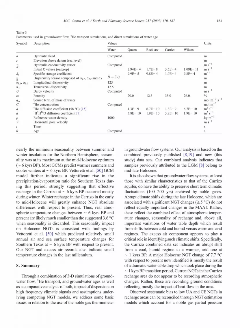
Table 3Parameters used in groundwater flow, 4He transport simulations, and direct simulations of water age

Symbol Description Values Units

Water Queen Recklaw Carrizo Wilcox

h Hydraulic head Computed mz Elevation above datum (sea level) m

K¼ Hydraulic conductivity tensor Computed m s−1

Initial K values (outcrop) 2.94E− 4 1.7E− 8 3.5E− 4 1.09E− 11 m s−1

Ss Specific storage coefficient 9.9E− 5 9.8E− 4 1.0E− 4 9.8E− 4 m−1

a¼ Dispersivity tensor composed of αL1, αL2 and αT D

¼ ¼ a¼U m

αL1, αL2 Longitudinal dispersivity 125 mαT Transversal dispersivity 12.5 mU Darcy velocity Computed m s−1

ω Porosity 20.0 12.5 35.0 26.0 %qm Source term of mass of tracer mol m−3 s−1

C 4He concentration Computed mol m−3

d 4He diffusion coefficient (58 °C) [15] 1.3E− 9 6.7E− 10 1.3E− 9 6.7E− 10 m2 s−1

d 1H3H16O diffusion coefficient [7] 3.8E− 10 1.9E− 10 3.8E− 10 1.9E− 10 m2 s−1

ρ Reference water density 1000 kg m−3

V Horizontal pore velocity m s−1

t Time sθ Age Computed s


nearly the minimum seasonality between summer andwinter insolation for the Northern Hemisphere, season-ality was at its maximum at the mid-Holocene optimum(∼ 6 kyrs BP). Most GCMs predict warmer summers andcooler winters at ∼ 6 kyrs BP. Vettoretti et al. [50] GCMmodel further indicates a significant rise in theprecipitation/evaporation ratio for Southern Texas dur-ing this period, strongly suggesting that effectiverecharge in the Carrizo at ∼ 6 kyrs BP occurred mostlyduring winter. Winter recharge in the Carrizo in the earlyto mid-Holocene will greatly enhance NGT absolutedifferences with respect to present. Thus, real atmo-spheric temperature changes between ∼ 6 kyrs BP andpresent are likely much smaller than the suggested 3.6 °Cwhen seasonality is discarded. This seasonality impacton Holocene NGTs is consistent with findings byVettoretti et al. [50] which predicted relatively smallannual air and sea surface temperature changes forSouthern Texas at ∼ 6 kyrs BP with respect to present.Our NGT and excess air records also indicate smalltemperature changes in the last millennium.

8. Summary

Through a combination of 3-D simulations of ground-water flow, 4He transport, and groundwater ages as wellas a comparative analysis of both, impact of dispersion onhigh frequency climatic signals and assumptions under-lying competing NGT models, we address some basicissues in relation to the use of the noble gas thermometer

in groundwater flow systems. Our analysis is based on thecombined previously published [8,19] and new (thisstudy) data sets. Our combined analysis indicates thatsamples previously attributed to the LGM [8] belong tomid-late Holocene.

It is also shown that groundwater flow systems, at leastthose with similar characteristics to that of the Carrizoaquifer, do have the ability to preserve short term climaticfluctuations (100–200 yrs) archived by noble gases.Abrupt climate shifts during the late Holocene, which areassociated with significant NGT changes (≥5 °C) do notreflect equally important changes in the MAAT. Rather,these reflect the combined effect of atmospheric temper-ature changes, seasonality of recharge and, above all,important variations of water table depth which resultfrom shifts between cold and humid versus warm and aridregimes. The excess air component appears to play acritical role in identifying such climatic shifts. Specifically,the Carrizo combined data set indicates an abrupt shiftfrom a cool, humid regime to a warmer, arid one at∼ 1 kyrs BP. A major Holocene NGT change of 7.7 °Cwith respect to present now identified is mostly the resultof a dramatic water table dropwhich took place during the∼ 1 kyrsBP transition period.CurrentNGTs in theCarrizorecharge area do not appear to be recording atmosphericchanges. Rather, these are recording ground conditionsreflecting mostly the impact of heat flow in the area.

Observed systematic bias to low UA and CE NGTs inrecharge areas can be reconciled through NGTestimationmodels which account for a noble gas partial pressure


increase in the unsaturated zone, potentially due to O2

depletion (OD model, [10]).

Acknowledgments

The authors wish to thank an anonymous reviewer forhis/her constructive comments as well as Dr. R. van derHilst for the editorial handling of this manuscript. Theauthors also thank E. T. Baker (USGS, Austin), J.-P. Nicot(Bureau of Economic Geology, Austin), R. E. Mace, G.Franklin, J. Hopkins (Texas Water Development Board,Austin), as well as L. Ackers, M. Mahoney, J. West, andC. Gonzales (Evergreen Underground Water Conserva-tion District, Pleasanton) for their help in providingadditional geological and hydrogeological information aswell as assistance with field sampling. Financial supportby the U.S. National Science Foundation grant EAR-03087 07 is greatly appreciated.

Appendix A

A.1. 3-D Model

A.1.1. Mathematical formulation and numericalapproach

To model groundwater flow and mass transport, twoclassical equations are solved. For incompressible fluids,the general 3-D diffusion equation is expressed as [31]:

jd K¼jh

� �¼ Ss

AhAt

ð1Þ

where K¼

is the hydraulic conductivity tensor, h is thehydraulic head, Ss is the specific storage coefficient, andt is the time. All symbols and values used in this sectionare defined in Table 3.

To account for advection, kinematic dispersion, andmolecular diffusion the 3-D transport equation isexpressed as:

jd D¼ þx d

¼� �jC−CU

Y� �¼ x

ACAt

þ qm ð2Þ

where UY

is the Darcy velocity, d¼is the pore diffusion

coefficient tensor of the solute in question, ω is theporosity, qm is a source term corresponding to the added orwithdrawn mass of tracer per unit volume per unit time,and C is the concentration of the solute in water. D

¼is the

dispersivity coefficient tensor.Movement of water in porous media is, in addition to

advection and like any other tracer, also affected by

kinematic dispersion, molecular diffusion, and cross-formational flow (e.g., [7,32,33]). 3-D groundwater agesimulations taking these processes into account werecarried out in steady-state and calculated as follows [32]:

jd a¼U þ x d

¼� �jh− hU

Y� �

¼ x ð3Þ

where θ is the age.All simulations were conducted with the finite

element code METIS [34] in steady-state.

A.1.2. Boundary conditions, calibration data andparameter values

Groundwater flow boundary conditions includehydraulic heads prescribed on the outcrop areas of allformations as well as on top of the Queen City aquiferobtained through geostatistical modeling [17]. A no-flow boundary condition was imposed both at the base ofthe Wilcox and lateral boundaries of the domain. Inaddition, a hydraulic conductivity of 10−5 m s−1 wasimposed in the Wilcox Geothermal Corridor area,allowing the water to be evacuated upward, reflectingthe situation occurring at the major growth–fault system.

For the transport model an ASW 4He concentration of2.01*10−6 mol m−3 was imposed on all outcrop areas. Ontop of the Queen City an outlet condition was prescribed,which allows 4He to be evacuated upward by advection. A4He flux representing the external contribution from theunderlying crust and/or mantle was imposed at the base ofthe Carrizo. This upward external flux is our 4He transportcalibration parameter. Inside the domain, a term represent-ing in-situ 4He production was imposed (cf., [12]).

To account for groundwater mixing, water age istreated in a similar manner to that of a solute concen-tration. Water age is simulated by considering the productof water mass (ρV) and age (θ) [32], where ρ is the waterdensity and V is the water volume. This quantity, referredto as “age mass”, is conserved and is equivalent to molesof a solute tracer. Boundary conditions included zero-agemass flux across all no flow and inflow boundaries of the3-D domain (Fig. 1b) and no age–mass dispersive fluxacross outflow boundaries.

Appendix B

B.1. Periodic versus discrete pulse signal response —mathematical formulation

The analysis presented below is not exhaustive andremains greatly simplified. A more thorough analysis onthe impact of dispersion on high versus low frequencyclimatic signals will be presented elsewhere.


We start by analyzing a periodic signal behavior, forexample, a fluctuation of noble gas concentrations in thewater table translating into NGT variations. Here, wedeal with a succession of peaks separated by a constanttime interval T (period). As time since the initial pulseincreases, partial superposition of the peaks will occur,leading to smoothing and eventually a loss of signal. Weanalyze this periodic signal behavior in a mono-dimensional (along x) groundwater flow system. Thedispersion equation is described by:

DA2CAx2

−VACAx

¼ ACAt

ð5Þ

where V is the horizontal pore velocity. The solution to abrief pulse (injection) is given by:

Cðx; tÞ ¼ m

2effiffiffiffiffiffiffiffikDt

p exp −ðx−VtÞ24Dt

!: ð6Þ

Where m is the initial mass of the solute andε kinematic porosity. This gaussian distributioncan be described by the width corresponding to thehalf-height of the peak concentration (Cmax/2) at a timet, here referred to as half-width. For example, ifexp − 12

4Dt

� �¼ 0:5, half-width ¼ 3:4

ffiffiffiffiffiDt

p. Two pulses

sent within a time interval T will remain separated onlyif the sum of their half-widths is much smaller than thedistance between their maxima (VT). This requirementfor a proper preservation of the signals can be expressedin terms of the dimensionless number CG as follows:

CG ¼ VTffiffiffiffiffiDt

p ¼ VTffiffiffiffiffiffiffiaVt

p ¼ VTffiffiffiffiffiffiaL

p ð7Þ

where L is the distance covered by the signal. Note that(CG)2, in addition to T2/t which directly relates thesignal period to the time since the first pulse occurred,incorporates also D/V2, the parameter on which Stuteand Schlosser [1] based their analysis. Incorporation ofT2/t renders CG dimensionless, thus, ideal for analysis ofthe signal's behavior. To identify the CG thresholdvalues for which the peak of a particular signal remainssharp, and that one for which it blends with neighboringsignals, the response to a sinusoidal injection was sim-ulated. The latter is given by the convolution integral:

Cðx; tÞ ¼Z t

0IðsÞ 1

2effiffiffiffiffiffiffiffiffiffiffiffiffiffiffiffiffikDðt−sÞp exp −

ðx−V ðt−sÞÞ24Dðt−sÞ

!ds

ð8Þ

where τ is time and I(τ)dτ is the tracer mass injectedduring time interval dτ:

IðtÞ ¼ V eðvm þ va � sinð2kt=TÞÞ ð9Þ

where Vε is the water flux, and vm and va are the averageand amplitude of the signal's fluctuation. Note that thissinusoidal signal is smoother than the succession of pulsesdiscussed above. After a certain distance, however, theshape of a short signal displays little dependence on itsinitial shape. Our simulations show that the signal is almostentirely lost for CG=2.5, while extremely sharp for CG=5.

Behavior of a discrete high-frequency pulse signal(e.g., an abrupt change in climate) is distinct and contrastsgreatly with that one of a periodic signal. To observe itspropagation over time a similar approach was used inwhich the signal corresponds to half a period, i.e., T/2.

References

[1] M. Stute, P. Schlosser, Principles and applications of the noblegas paleothermometer, in: P.K. Swart, K.C. Lohmann, J.A.McKenzie, S. Savin (Eds.), Climate Change in ContinentalIsotopic Records, Geophysical Monograph, vol. 78, AGU, 1993,pp. 89–100.

[2] M. Stute, P. Schlosser, Atmospheric noble gases, in: P.G. Cook,A.L. Herczeg (Eds.), Environmental Tracers in SubsurfaceHydrology, Kluwer, Dordrecht, 1999, pp. 349–377.

[3] R. Kipfer, W. Aeschbach-Hertig, F. Peeters, M. Stute, Noblegases in lakes and ground waters, Noble Gases in Geochemistryand Cosmochemistry, Rev. Min. and Geochem., vol. 47,Mineralogical Society of America, Washington, D.C., USA,2002, pp. 615–700.

[4] M. Stute, C. Sonntag, Palaeotemperatures derived from noblegases dissolved in groundwater and in relation to soiltemperature, Panel Proceedings Series STI/PUB/859, IAEA,1992, pp. 111–122.

[5] W. Aeschbach-Hertig, M. Stute, J.F. Clark, R.F. Reuter, P.Schlosser, A paleotemperature record derived from dissolvednoble gases in groundwater of the Aquia Aquifer (Maryland,USA), Geochim. Cosmochim. Acta 66 (5) (2002) 797–817.

[6] F.M. Phillips, M.C. Castro, Groundwater dating and residence-time measurements, in: J.I. Drever (Ed.), Surface and GroundWater, Weathering, and Soils, Treatise on Geochemistry, vol. 5,Elsevier, Oxford, UK, 2003, pp. 451–497.

[7] M.C. Castro, P. Goblet, Calculation of ground water ages — acomparative analysis, Ground Water 43 (3) (2005) 368–380.

[8] M. Stute, P. Schlosser, J.F. Clark, W.S. Broecker, Paleotempera-tures in the Southwestern United States derived from noble gasesin ground water, Science 256 (5059) (1992) 1000–1001.

[9] L. Ma, M.C. Castro, C.M. Hall, A late Pleistocene–Holocene noblegas paleotemperature record in southern Michigan, Geophys. Res.Lett. 31 (23) (2004) L23204, doi: 10.1029/2004GL021766.

[10] C.M. Hall, M.C. Castro, K.C. Lohmann, L. Ma, Noble gases andstable isotopes in a shallow aquifer in southern Michigan:implications for noble gas paleotemperature reconstructions forcool climates, Geophys. Res. Lett. 32 (18) (2005) L18404,doi: 10.1029/2005GL023582.

http://dx.doi.org/10.1029/ 2004GL021766

http://dx.doi.org/10.1029/2005GL023582


[11] W. Aeschbach-Hertig, F. Peeters, U. Beyerle, R. Kipfer,Paleotemperature reconstruction from noble gases in groundwater taking into account equilibration with entrapped air, Nature405 (6790) (2000) 1040–1044.

[12] M.C. Castro, D. Patriarche, P. Goblet, 2-D numerical simulationsof groundwater flow, heat transfer and 4He transport —implications for the He terrestrial budget and the mantlehelium–heat imbalance, Earth Planet. Sci. Lett. 237 (3–4)(2005) 893–910, doi: 10.1016/j.epsl.2005.06.037.

[13] M.C. Castro, P. Goblet, Noble gas thermometry and hydrologicages: evidence for late Holocene warming in Southwest Texas,Geophys. Res. Lett. 30 (24) (2003) 2251, doi: 10.1029/2003GL018875.

[14] L.Mercury, D.L. Pinti, H. Zeyen, The effect of the negative pressureof capillary water on atmospheric noble gas solubility in groundwater and palaeotemperature reconstruction, Earth Planet. Sci. Lett.223 (1–2) (2004) 147–161, doi: 10.1016/j.epsl.2004.04.019.

[15] G. Favreau, A. Guero, J.L. Seidel, Comment on “Improvingnoble gas based paleoclimate reconstruction and groundwaterdating using 20Ne/22Ne ratios,” by F. Peeters et al. Geochim.Cosmochim. Acta 67 (2003) 587–600;Geochim. Cosmochim. Acta 68 (6) (2004) 1433–1435,doi: 10.1016/j.gca.2003.07.022.

[16] M.C. Castro, P. Goblet, Calibration of regional groundwater flowmodels: working toward a better understanding of site-specificsystems, Water Resour. Res. 39 (6) (2003) 1172, doi: 10.1029/2002WR001653.

[17] D. Patriarche, M.C. Castro, P. Goblet, Large-scale hydraulicconductivities inferred from three dimensional groundwater flowand 4He transport modeling in the Carrizo aquifer, Texas,J. Geophys. Res. 109 (B11) (2004) B11202, doi: 10.1029/2004JB003173.

[18] D. Patriarche, M.C. Castro, P. Goovaerts, Estimating regionalhydraulic conductivity fields— a comparative study of geosta-tistical methods, Math. Geol. 37 (6) (2005) 587–613,doi: 10.1007/s11004-005-7308-5.

[19] M.C. Castro, M. Stute, P. Schlosser, Comparison of the 4He agesand 14C ages in simple aquifer systems: implications forgroundwater flow and chronologies, Appl. Geochem. 15 (2000)1137–1167.

[20] D.G. Bebout, V.J. Gavenda, A.R. Gregory, S.C. Claypool, J.H.Han, J.H. Seo, Geothermal resources, Wilcox Group, Texas GulfCoast, Bur. of Econ. Geol., Univ. of Tex. at Austin, Austin, Tex.,USA, Report ORO/4891-3, 1978, 82 pp.

[21] H.S. Hamlin, Depositional and ground-water flow systems of theCarrizo–Upper Wilcox, South Texas, Report of Investigations,vol. 175, Bur. of Econ. Geol., Austin, Tex., USA, 1988, 61 pp.

[22] H.B. Harris, Ground-water resources of La Salle and McMullenCounties, Texas, Bulletin, vol. 6520, Texas Water Commission,Austin, Tex., USA, 1965, 96 pp.

[23] W.H. Alexander Jr., D.E. White, Ground-water resources ofAtascosa and Frio Counties, Texas, Report, vol. 32, Texas WaterDevelopment Board, Austin, Tex., USA, 1966, 211 pp.

[24] M.O. Saar, M.C. Castro, C.M. Hall, M. Manga, T.P. Rose,Quantifying magmatic, crustal, and atmospheric helium contribu-tions to volcanic aquifers using all stable noble gases: implica-tions for magmatism and groundwater flow, Geochem. Geophys.Geosyst. 6 (2005) Q03008, doi: 10.1029/2004GC000828.

[25] T. Torgersen, W.B. Clarke, Helium accumulation in groundwater,I: an evaluation of sources and the flux of crustal 4He in the GreatArtesian Basin, Geochim. Cosmochim. Acta 49 (5) (1985)1211–1218.

[26] M.C. Castro, A. Jambon, G. deMarsily, P. Schlosser, Noble gases asnatural tracers of water circulation in the Paris Basin 1. Measure-ments and discussion of their origin and mechanisms of verticaltransport in the basin,WaterResour. Res. 34 (10) (1998) 2443–2466.

[27] M.C. Castro, P. Goblet, E. Ledoux, S. Violette, G. de Marsily,Noble gases as natural tracers of water circulation in the ParisBasin 2. Calibration of a groundwater flow model using noblegas isotope data, Water Resour. Res. 34 (10) (1998) 2467–2483.

[28] T.H.E. Heaton, J.C. Vogel, “Excess air” in groundwater,J. Hydrol. 50 (1–4) (1981) 201–216.

[29] C.J. Ballentine, C.M. Hall, Determining paleotemperature andother variables by using error-weighted, nonlinear inversion ofnoble gas concentrations in water, Geochim. Cosmochim. Acta63 (16) (1999) 2315–2336.

[30] M.C. Castro, Helium sources in passive margin aquifers — newevidence for a significant mantle 3He source in aquifers withunexpectedly low in-situ 3He/4He production, Earth Planet. Sci.Lett. 222 (3–4) (2004) 897–913, doi: 10.1016/j.epsl.2004.03.031.

[31] G. de Marsily, Quantitative Hydrogeology, Academic Press, SanDiego, CA, USA, 1986 440 pp.

[32] D.J. Goode, Direct simulation of groundwater age, Water Resour.Res. 32 (2) (1996) 289–296.

[33] M. Varni, J. Carrera, Simulation of groundwater age distribution,Water Resour. Res. 12 (34) (1998) 3271–3281.

[34] E. Cordier, P. Goblet, Programme METIS- Simulation d'écoule-ment et de transport miscible en milieu poreux et fracturé, Centred'Informatique Géologique, Ecole Nationale Supérieure desMines de Paris, Fontainebleau, France, Notice d'emploi LHM/RD/99/18, 1999.

[35] C.E. Manning, S.E. Ingebritsen, Permeability of the continentalcrust; implications of geothermal data and metamorphic systems,Rev. Geophys. 37 (1) (1999) 127–150.

[36] W.B. Klemt, G.L. Duffin, G.R. Elder, Ground-water Resourcesof the Carrizo Aquifer in the Winter Garden Area of Texas,Report, vol. 210 (1), Texas Water Development Board, Austin,Tex., USA, 1976, 30 pp.

[37] LBG-Guyton Associates, HDR Engineering Inc., InteractionBetween Ground Water and Surface Water in the Carrizo–Wilcox Aquifer, Texas Water Development Board, 1998W600.8 C235.

[38] W. Aeschbach-Hertig, U. Beyerle, J. Holocher, F. Peeters, R.Kipfer, Excess air in groundwater as a potential indicator of pastenvironmental changes, Study of Environmental Change usingIsotope Techniques, IAEA, Vienna, 2002, pp. 174–183.

[39] Texas Water Development Board, Ground-Water Database, http://www.twdb.state.tx.us/publications/reports/GroundWaterReports/GWDatabaseReports/GWdatabaserpt.htm, 2003.

[40] K.H. Tan, Environmental Soil Science; Second Edition, Revisedand Expanded, Marcel Dekker, New York, NY, USA, 2000451 pp.

[41] S.A. Hall, Channel trenching and climatic-change in the SouthernUnited-States Great-Plains, Geology 18 (4) (1990) 342–345.

[42] M.D. Blum, S. Valastro Jr., Response of the Pedernales River ofcentral Texas to late Holocene climatic change, Ann. Assoc. Am.Geogr. 79 (3) (1989) 435–456.

[43] D.A. Hodell, J.H. Curtis, G.A. Jones, A. Higueragundy, M.Brenner, M.W. Binford, K.T. Dorsey, Reconstruction ofCaribbean climate change over the past 10,500 years, Nature352 (6338) (1991) 790–793.

[44] D.A. Hodell, M. Brenner, J.H. Curtis, T. Guilderson, Solarforcing of drought frequency in the Maya lowlands, Science 292(5520) (2001) 1367–1370.

http://www.twdb.state.tx.us/publications/reports/GroundWaterReports/GWDatabaseReports/GWdatabaserpt.htm




http://dx.doi.org/10.1029/2003GL018875


http://dx.doi.org/10.1016/j.gca.2003.07.022

http://dx.doi.org/10.1029/2002WR001653

http://dx.doi.org/10.1029/2004JB003173

http://dx.doi.org/10.1007/s11004-005-7308-5

http://dx.doi.org/10.1029/2004GC000828



[45] R.B. Gill, The Great Mayan Droughts: Water, Life, and Death,University of New Mexico Press, Albuquerque, 2000 464 pp.

[46] G.B. Wilson, G.W. McNeill, Noble gas recharge temperatures andthe excess air component, Appl. Geochem. 12 (6) (1997) 747–762.

[47] J.E. Brinkman,Water age dating of the Carrizo sand, Ph.D., Univ.of Arizona (1981) 131 pp.

[48] G.D. Smith, F. Newhall, L.H. Robinson, D. Swanson, Soil-temperature regimes — their characteristics and predictability,Technical Publication, vol. 144, U.S. Department of AgricultureSoil Conservation Service, 1964, 14 pp.

[49] N.M.J. Hall, P.J. Valdes, A GCM simulation of the climate6000 years ago, J. Clim. 10 (1) (1997) 3–17.

[50] G. Vettoretti, W.R. Peltier, N.A. McFarlane, Simulations of mid-Holocene climate using an atmospheric general circulationmodel, J. Clim. 11 (10) (1998) 2607–2627.

[51] A. Kitoh, S. Murakami, H. Koide, A simulation of the LastGlacial Maximum with a coupled atmosphere–ocean GCM,Geophys. Res. Lett. 28 (11) (2001) 2221–2224.

[52] Z. Liu, S.P. Harrison, J. Kutzbach, B. Otto-Bliesner, Globalmonsoons in the mid-Holocene and oceanic feedback, Clim. Dyn.22 (2–3) (2004) 157–182, doi: 10.1007/s00382-003-0372-y.

http://dx.doi.org/10.1007/s00382-003-0372-y

a new noble gas paleoclimate record in texas — basic assumptions revisited

Documents