A New Keynesian Model with Noisy

Observations of Aggregate Variables

Dennis Tatarkov

September 21, 2011

Abstract

This thesis looks at the effects of data uncertainty on the representativeconsumer DSGE model. Several cases are considered: demand/supplyshock as well as the effects on policy. A measure of welfare is approximatedfrom the assumed utility function. Using a set of parameter values, thewelfare effects of a range of noise levels is calculated. The results implya strongly non-linear effect of uncertainty on welfare. Optimal filteringplaces more weight on the variable which is subject to less noise. Hence ina regime where the inflation rate is affected by both the cost-push shockand an informational error term, the utility of this indicator is found todecline very rapidly. Policy acts on the perceived shocks, so that in thepresence of policy the two indicators become orthogonalized.This leads toa situation where only improvements in the measurement of the outputgap positively affect welfare.

1 Introduction

A feature of the real world which is often overlooked in economic modeling isthe presence of uncertainty regarding the true economic variables. The aim ofthis paper is to incorporate elements of this uncertainty through additive noiseinto a DSGE model that has become standard in the literature. This is donethrough re-examination of the first order conditions under partial information.The results are then used to assess the welfare costs which are imposed onsociety by a lack of access to complete and accurate information the economy.

The effects of this uncertainty have been recognized by policymakers at theBank of England, who in their output projections have placed error bars ontopast observations of GDP. Retrospective revisions of GDP data are also frequent,some of these occur after several years of the release of the initial estimate.Similarly, it is also widely recognized that measures of inflation have inherentproblems, such as an inability to take into account the substitution effect or aninsufficient adjustment for the quality of manufactured goods. Unlike the datafor GDP, inflation data is never revised. However, due to substitution in theconsumption basket, introduction of new goods and changes in the quality ofgoods already being consumed, the measured rate of inflation is never a perfectlyaccurate measure of the price changes in the basket of consumption goods andit is reasonable to assume that some noise is present in this measure. Thisthesis focuses on the effects of this uncertainty in a standard DSGE model, andleading from this onto the effects that uncertainty has on welfare as measuredby the level of utility of a representative household.

In terms of the DSGE model, the measure of the inflation rate is relevantto producers to determine the pricing strategy that they follow since in the im-perfectly competitive setting that is considered here, the relevant price statisticis the ratio of own price to the general price level. Since a Dixit-Stiglitz con-sumption aggregate is used, the overall price level is the relevant metric forcompetitor prices. Therefore, the noise in the measure of inflation could be seenas the effect of not knowing how the economy-wide inflation measure translatesinto a relevant metric of competitor prices.

The way that this paper is organized is as follows. The first section providesa literature review and places this model among the recent developments inmacroeconomics, the next section details the model and calculates welfare lossesas well as providing some numerical estimates. The final section concludes.

2 Literature Review

The most well-known model to deal with an imperfect information among mar-ket participants, and the macroeconomic implications of such an information

2

structure has been the Lucas islands model (1972, 1973, 1975). The model isbased on an idea that the economy consists of some number of islands, whichin one formulation is a continuum between 0 and 1. These Islands are taken tobe separate, which allows for the markets to be both physically and informa-tionally separate. There is only one consumption good, which is produced andtraded competitively on each island. In this setting, each island is subject to amean zero idiosyncratic shock, while at the same time the economy experiencesa shock to the level of the overall money supply. After each period individualsare randomly reassigned to another island. Since the cash balances that theyhold depreciate at the rate of inflation in the overall economy, this means thatdespite being physically separate from the rest of the economy, their decisionsare affected by the aggregate price level that prevails in the set of islands whichcomprise the economy. As each individual is allocated to another island at ran-dom, in expectation all goods are perfectly substitutable and are defined as agood belonging to a particular island.

This model focuses on the aggregate supply side of the economy and is aattempt at an explanation behind the apparent failure of monetary neutralityin the short run. The model can be summarized using a few key equations. Theessential idea is that rational agents are placed into a setting where they areconcerned with relative prices, yet unable to distinguish relative from generalprice movements. At the simplest level, Lucas assumes that the supply yt ineach market i depends on the ratio of the price in that market to the generalprice level as:

yt (i) = κ (pt (i)− E (pt|It)) (1)

Here, p denotes the (log of) the price level and y denotes output with indi-vidual market price being given by terms with the market index i as a functionaldefinition. To complete the model, Lucas assumed that the general price levelis unobserved and follows a stochastic path, the distribution of which is knownto all participants. Furthermore, there is an additional shock process on theindividual prices follows the following:

pt (i) = pt + z (2)

Assuming that the z term is stochastic and follows a known distributionallows for a filtering problem to be set up for the expectation of the generalprice level. In that case, the responsiveness to that expectation will dependon the signal-to-noise ratio of relative price to aggregate shifts. Therefore, theexpectation in the firm supply function is given by:

3

E (pt|It) = E (pt|pt (i)) (3)

= κpt (i)

Here, κ is the signal-to-noise ratio which has the form of:

κ =σ2z

σ2z + σ2

τ

(4)

The variance of the general price level is given by σ2τ which stands as a magni-

tude of the size of the general shock affecting the economy. In this case, σ2z is the

idiosyncratic shock to the individual firm’s markets. Putting all this togetherand summing across the distribution of firms across i allows the derivation ofthe well-known Lucas supply function:

yt = κκpt (5)

In keeping with notation later, the hat over the output term signifies a gapfrom the competitive allocation. This states that in response to a price increasein the local market, the firm will only raise price a portion of the way of thatincrease. The structure of the κ multiplier is such that if all shocks are due tothe aggregate and σ2

z is large relative to σ2τ , then most of the shock will be taken

up by prices and vice versa.

This model is one of the first which uses incomplete information as a causebehind incomplete adjustment, although the particular focus of the problem isnot framed in terms of informational errors, but rather a lack of it altogether.Following it’s publication this model attracted criticism for it’s inability to ex-plain deviations from the flexible price equilibrium which last longer than thedelay in publishing the economy-wide aggregate data. As this is released with alag of only a month to a quarter, this model fails in explaining deviations witha periodicity of a year or more.

Since the publication of the Lucas model, several others have proposed al-ternative monetary policy transmission mechanisms based on uncertainty andbeliefs, while responding to the criticism of insufficient persistence. These havetended to depart from the original idea of uncertainty about current data, asit tends to be released relatively frequently. This does not lead to any sig-nificant sources of internal persistence of shocks apart from those generatedthrough assumptions on the shock process itself. Woodford (2001) proposes anidea that given that information is incomplete means that second order beliefswould be relevant to decision making. The key changes that allow this to be

4

relevant are the assumptions of monopolistic competition between firms whichallows price-setting to take place as well as a limit on the agents’ ability toprocess information. The general result is that since second-order beliefs aremore sticky, hence leading to greater internal model persistence. It is foundthat this mechanism can in some cases approximate that of the more standardCalvo contracts.

Similarly, Aoki (2007) looks at the effects of uncertainty about the bank’sinflation target as a key informational handicap for economic agents. In thepresence of stochastic disturbances, private agents cannot determine whether ashift in the real rate is caused by a shock, or whether that signifies a changein the bank’s target rate, both of which are unobservable. Without a crediblecommitment mechanism, a situation arises where shocks are imperfectly ob-served, and the variation in the natural rate is only partially attributed to theseshocks. This imperfect credibility leads to incomplete adjustment in responseto shocks in a similar vein to the Lucas model, however rather than dependingon informational imperfections the key mechanism here is learning. Learningon behalf of the private sector which leads to greater credibility of the infla-tion target rate, which means that some amount of time is needed before thetarget becomes more credible, diminishing the volatility of transmitted shocks.Both these models continue to employ information as the driving mechanismfor incomplete adjustment.

Instead of letting the informational imperfections play a key role in breakingmonetary neutrality, it has become more common to assume the presence ofnominal rigidities, which force producers to set prices away from the flexible-price equilibrium. This has been motivated firstly by the observation that pricesare never set in a continuous manner, with revisions only occurring at regularintervals. Furthermore, it is commonly observed that wages are set at intervalsof 1-2 years. To provide rigorous micro-foundations, this behaviour is usuallyrationalised by taking into account the existence of small menu costs, whichnevertheless induce agents to only change prices infrequently. This strand hasseparated into state-dependent and time-dependent pricing rules. While a state-dependent pricing rule is obviously superior in terms of it’s micro-foundations,the complexity of such rules prohibits a model from achieving parsimony. Thisstems from the fact that state-dependent pricing rules result in a strong historydependence, with each successive pricing decision becoming dependent on astring of past realisations.

The introduction of Calvo pricing means that the model has an appearancewhich is similar to more contemporary formulations. This sets a constant hazardrate for pricing decisions and while potentially some prices can be set for anunlimited time period, the average duration of a price contract is given by theinverse of the hazard rate. With this value calibrated to that observed in thewider economy would allow for a realistic portrayal of the rigidities present inthe economy. This approach also has limitations. While it can be argued that

5

a constant hazard rate is appropriate for a situation where inflation is largelystable, this would not be the case for countries which experience periods of veryhigh and volatile inflation. In this case, price changes would be carried out withgreater frequency, i.e. the parameter for the hazard rate could no longer beapproximated to be constant.

The basic model itself owes much of it’s structure to the model exposited inChapter 3 of Woodford (2003), while assuming some particular, though com-mon functional forms for simplicity of exposition. Solution is then achieved bylog-linear approximations around the steady state of the economy. Woodfordpresents a general model of an economy with a representative household, whichis subjected to a vector of stochastic disturbances. Using the utility functionof the representative consumer, the author is able to derive a second order ap-proximation to the welfare function of the economy. This welfare function isoutwardly similar to the more standard ad hoc assumption of a loss function(Clarida, Gali, Gertler, 1999) for the central bank dependent on the square ofthe deviations of the level of output and the inflation rate. The presence ofthe squared output gap term results from the curvature of the utility function,with greater variance leading to reductions in the average level of utility. In-flation penalizes the welfare function due to distortions in the price level. Thederivation of the welfare function shows this result to be highly dependent onthe time-dependent pricing rule that the model employs. The essential intuitionstates that higher rates of inflation lead to larger gaps in the pricing betweenfirms who are able to adjust in the current period and those that set their pricesin one of the previous periods. This causes some resource mis-allocation asprices set by firms in the past period no longer reflect the marginal costs ofproducing those goods. This micro-foundation for the costs of inflation dependson the form of the pricing rigidity. A situation could be envisaged where if allfirms adjust their prices simultaneously, even with some delay, then inflationcauses no utility loss. Furthermore, this derivations for the costs of inflationdraws some criticism from the observation that higher inflation is associatedwith greater volatility in the inflation. As this makes long term contracts (suchas employment contracts) more risky, this imposes costs on individuals. Thissource of disutility is not adequately reflected in the standard DSGE model.

In making the welfare derivation Woodford goes on to assume that the econ-omy’s inefficiency tends to zero, so that the central bank does not have anincentive to try to push output beyond it’s natural rate in the sense of Gordonand Barro model. In another paper Benigno and Woodford (2005) explore anapproximation which does not rely on either making an assumption regardingthe size of the distortion, or an assumption that such a distortion is offset by anappropriate fiscal policy. They show that this results in a modification of theweights attributed to inflation and output in the welfare function.

The baseline model, as presented by Woodford, is then supplemented in mysetting by a set of informational imperfections, essentially making agents work

6

with imperfect data. The paper, which has provided much of the motivation be-hind the interest in informational imperfections has been a paper by Orphanides(1997). In this paper, the author looks at a specification of the popular Taylorrule using contemporaneous data estimates and finds that this differs from therule that emerges from data of varying vintages. While this paper does not di-rectly test whether initial indicator estimates are subject to noise and the degreeof error that this entails, the paper does indicate a large discrepancy betweenthe policy interest rate which is set according to contemporaneous and reviseddata.

It can be argued that from the outset, the baseline model considered hereis insufficiently detailed to be able to handle information uncertainty, as theassumption of a representative consumer rules out any heterogeneity in theresponse of the private sector. Aoki (2006b) explores the micro-foundations be-hind informational constraints. The author considers a model of islands, whereinformation is dispersed among agents in the economy. The essential structuremeans that each agent is only able to observe the activity of those islands thatare nearest to him rather than aggregate information. This leads to a situationwhere none of the agents have reliable information about the true state of theeconomy. It is then shown that this model behaves in an identical manner to amodel with a representative consumer, where the consumer has full informationwhile the monetary authority only has only partial information about the econ-omy. This can be seen as an argument against the assumption used here aboutthe symmetry of informational noise, however the type of uncertainty consideredin this paper does not correspond to the idea of errors in aggregate data, whichis relevant for economy-wide decision making. On the other hand, followingthis model, shows that the effects of idiosyncratic uncertainty are likely to besmall and the assumption of a representative consumer is warranted, which isinherited from the full information baseline model.

Several papers also look at the theoretical implications of informational noisefor policy formulation. Aoki (2006a) makes an assumption that the privatesector is fully informed, while the central bank has only partial informationabout current indicators. In this setting data is revised within one period to it’strue values. This is the opposite assumption to the setting considered previouslyand focuses on the filtering and optimisation problem of the monetary authority.Aoki derives the optimal commitment solution using a Kalman filter to takeaccount of both filtering and optimal control. The findings show that initialresponses are likely to overshoot the value in the next period. Policy here isfound to closely resemble that under price-level targeting. Similarly, Svenssonand Woodford (2002) consider the form of the solution in a model where partialinformation is available. They detail the conditions where certainty equivalenceholds for the optimal reaction function, as well as a situation where optimizationand filtering cannot be made separate. These papers impose the condition thatthe information set of the central bank is a subset of the information set of thepublic. This means that the effect of partial information on household decisions

7

is not considered.

Additionally, McCallum (2001) has written on the implications of outputgap mis-measurement if the Central bank follows a policy rule, but insteadof using the true economic output gap, defined as the difference between thecurrent level of output and the level of output that prevails in steady state, thebank has an incorrect measure. This possibility translates to model uncertaintyas the optimal policy in any particular case depends on the specification ofthe model economy, it is necessary to have some general policy prescriptionswhich would be applicable to a large set of candidate models. For this reason,McCallum argues against a strong response to output data, partially groundinghis argument in the observed uncertainty of the output gap.

With this, I have chosen to simplify the set-up as much as possible, whileretaining the key elements of the DSGE model. This means that I will not beconcentrating on the possible gains from commitment and will rather follow asimpler discretionary policy framework. Similarly, the shock structure will alsobe simplified from that adopted in Clarida, Gali and Gertler as I will only focuson one-period transitory shocks. With most of the set-up following the lines ofWoodford chapter 2 model, this work will take particular functional forms forease of exposition.

3 Households

The model is based around a set of standard assumptions and this section detailsthe description of the household. The individual household’s utility, U is givenby:

U = E0Σ∞s=0βsUt+s (6)

where

Ut = Nt(C1−δt

1− δ− Lγt

γ); (7)

Ct = (

∫ 1

0

Ct (i)θ−1θ di)

θθ−1 ;Lt =

∫ 1

0

Lt (i) di (8)

log(Nt) = nt˜N(0, σ2n) (9)

8

Here, C denotes consumption and L denotes labour input, with functionalarguments referring to the quantity for a given good. Consumption is modeledusing a Dixit-Stiglitz aggregator where consumption goods are located on thecontinuum between 0 and 1. Each of the goods is produced by a separate firm,which employs labour from the household. The overall labour disutility of thehousehold is determined by a simple sum of the labour supplied to each firm.

The form of the utility function implies that it is additively separable overtime, which serves to rule out some realistic features such as habit formation.In the event that habit formation was included in the description, the house-hold optimization would yield a more persistent pattern for consumption, whichwould have served as an integral mechanism for generating persistence. At thesame time, there is a preference shock modeled by Nt, which has a log-normaldistribution around zero with a variance of σ2

n.This term denotes a demandshock that is introduced into the economy.

The household also faces a budget constraint, where At , is the holding ofgovernment assets with a nominal interest rate set by the central bank at timet.

At−1Pt

(1 + it−1) + LtWt

Pt+ Πt −

∫ 1

0

Ct (i)Pt(i)

Ptdi− At

Pt= 0 (10)

Maximizing the households utility subject to the constraint results in thefollowing set of first order conditions with a Lagrange multiplier λt:

At : −λt1

Pt+ Et

(λt+1

1 + itPt+1

)= 0 (11)

Lt : NtLγ−1t − λt

Wt

Pt= 0 (12)

Ct(i) : Nt(C−δt

∂Ct∂Ct (i)

)− λtPt (i)

Pt= 0 (13)

where

∂Ct∂Ct (i)

=

(Ct (i)

Ct

)− 1θ

(14)

since λt is the same for all goods it is possible to derive demand curves fromthese equations as follows.

9

Nt

(C−δt

(Ct (i)

Ct

)− 1θ

)− λt

Pt (i)

Pt= 0 (15)

λt =NtPtPt (i)

(C−δt

(Ct (i)

Ct

)− 1θ

)for all i ∈ [0, 1] (16)

Pt(k)

Pt (i)=

(Ct (k)

Ct(i)

)− 1θ

(17)

Ct (i) = Ct

(Pt(i)

Pt

)−θ(18)

Since there is no capital in the model, total output must equal total con-sumption, therefore this can be re-written as:

Yt (i) = Yt

(Pt(i)

Pt

)−θ(19)

According to this equation, demand for individual goods is proportional tothe total level of demand as well as the ratio of the price of the good relativeto the overall price level. The parameter θ, determines elasticity of substitutionbetween goods, and as such controls the degree of monopoly power that eachindividual producer enjoys.

3.1 Euler Equation

Using the demand curves above to substitute for λt, gives λt, = NtC−δt . Hence

it becomes possible to derive the following Euler equation for this household:

NtC−δt

Pt= Et

(Nt+1C

−δt+1

1 + itPt+1

)(20)

This can then be used to derive the IS curve for this model economy. Inorder to derive the IS curve, log-linearise the model around the steady statewith a value for the shock equal to it’s expectation. For all the variables which

10

correspond to this steady state, let them be denoted by letters with no sub-scripts. Using lower-case letters to denote the log of a variable and using hatsto denote gaps, such that for any variable, say X:

Xt −XX

' log (Xt)− log (X) = xt − x = xt (21)

A log-linearised relation of this type leads to the following form of the IScurve, which has become standard in the literature.

yt = Etyt+1 −1

δ(it − Etπt+1) + nt (22)

Essentially this relation states that the current output gap depends entirelyon the expectation of the output gap in the next time period, the gap betweenthe current interest rate and the inflation rate expected to prevail in the futureand lastly, the current output gap depends on the value of the ”preference”shock Nt, which affects the marginal value of utilities between periods, henceleads the household to shift consumption between time periods.

One of the shortcomings of the structure of an IS curve such as that presentedabove is that decisions on consumption in the current period depend almostentirely on expectations of the future. On the scale that time periods represent,which in this case corresponds to quarters, adjustment is instantaneous. Somemore recent models incorporate the effects of habits on the form of the aboveequation, which leads to some dependence on lagged values and smooths theadjustment process for households. This step has been avoided in this caseto simplify the overall set-up to focus on the effects of informational problemsalone.

3.2 Labour Supply

Using the definition of λt, = NtC−δt , the real marginal cost of labour is equated

to the real wage:

Wt

Pt= Lγ−1t Cδt (23)

The labour market functions competitively with both the household and thefirms acting as price-takers. Households supply an amount of undifferentiatedlabour equal to Lt which is employed by firms on the unit interval in amounts

11

Lt (i). Since the production function for firm i is Yt(i) = Lt(i), and Lt =∫ 1

0Lt (i) di, then to a first approximation lt = yt. Due to there being no capital

accumulation, Ct = Yt. The real marginal cost of output then depends entirelyon the output gap.

3.2.1 Supply Shocks

The way that the model is formulated allows supply shocks to be introducedwith relative ease into the model. Suppose that the per-period utility functionhas the following form:

Ut = Nt(C1−δt

1− δ− MtL

γt

γ) log (Mt) ˜N

(0, σ2

m

)(24)

The only difference from the baseline case is that there is an additional mul-tiplicative term on the dis-utility of labour. As with the time preference shock,suppose that the logarithm of Mt (denoted by mt) has a normal distributionwith a zero mean and a known variance of σ2

m.

This shock is motivated to take the form of a cost-push shock by creating agap between the wage rate and the marginal dis-utility of labour. It is importantto note, that while in form this can be seen as a real shock, the effect of Mt doesnot shift the natural rate of output in the same way that a productivity shockor preference shock would. In that sense this appears to be similar in form tothose shocks, but must be seen as conceptually different.

This modification leads to the following first order condition for labour:

Lt : NtMtLγ−1t − λt

Wt

Pt= 0 (25)

As before, λt = C−δt Nt. Therefore, the level of the real wage must now beequal to the following expression:

Wt

Pt= MtL

γ−1t Cδt (26)

This expression shows that the form of the real wage is broadly the same,although there is now a stochastic component to the level of the dis-utility oflabour. The baseline model is simply nested within this modification as a modelwhere σ2

m → 0. This now means that firms’ costs which consist of the real cost

12

of labour to households now also contains a stochastic component. This canroughly be interpreted as the variation in the real production costs. Therefore,this is a cost-push shock, which means that firms will have an incentive to passit onto prices, generating a burst of inflation.

4 Steady State

This section characterises the steady state of the economy described here, apoint around which all of the log-linear expansions are calculated. As describedin the previous sections, all firms are symmetrical, hence in the steady statethey all produce output at the same level as one another. Both the inflationrate and the output gap are equal to zero in the steady state defined here.In this symmetric steady state all firms demand identical quantities of labourfrom the household, face identical costs and set identical prices as a mark-upover the marginal cost determined by their degree of market power. Using thischaracterisation of the steady state the optimal pricing equation becomes:

N = 1, M = 1

P ∗

P= 1 =

(θ

θ − 1

)W

P(27)

Using the labour supply equation from above, the real wage rate must satisfy:

W

P= Lγ−1Cδ (28)

Now, as the model features no capital, C = Y. Also, consider the steadystate equivalent of L, given the fact that L(i) is a constant.

L =

∫ 1

0

L (i) di = L

∫ 1

0

di (29)

This then leads to the following result concerning the steady state level ofoutput.

Y = (θ − 1

θ)

1δ+γ−1 (30)

13

This is the level of output that prevails when the economy is not subjectto any shocks. The way that the supply shock has been introduced in thefirst section means that the shock to the dis-utility of labour does not have aneffect on the natural output level of the economy. If this took the form of aproductivity shock, then, the stochastic term would enter into the specificationof the steady state. As this would shift the natural rate by the same amount asthe actual output expansion, this would not enter the Phillips curve additively.Under the cost-push structure of the shock described above, the steady statelevel of output Y, remains the competitive equilibrium of the economy.

5 Firms

Firms are assumed to optimize their expected level of profit in every period.Consider the two cases: one where firms are free to set prices every period andanother case where firms are constrained with a Calvo pricing scheme.

5.1 Flexible Pricing

Firstly, consider a situation where all firms can change their prices in every pe-riod to maximize the discounted present value of profits. It is assumed that firmsare located on the unit interval indexed by i and hire labour from a competitivelabour market. Capital is absent and labour is the only factor of production.Labour required between firms is not specialized and the index i denoted thedemand for labour by firm i. Firms face a technological constraint in the formof the production function:

Yt(i) = Lt(i) (31)

As profit maximization is independent between time-periods, optimizationentails period-by period profit maximisation. Given the production functionabove and the demand function derived from household optimization results inthe following profit function for firm i:

Πt = (Pt (i)−Wt)Yt (i)

Pt(32)

where

14

Yt (i) = Yt

(Pt (i)

Pt

)−θ(33)

This expression is optimized with respect to the price set by an individualfirm to give the first order condition of the form:

Pt(i) =θ

θ − 1Wt (34)

The first order condition shows that the price set by an individual firm willbe held as a constant mark-up over costs, as typified by the wage rate. At thesame time, since all firms are assumed to be symmetrical, then this first ordercondition applies to all firms, and the equilibrium of this economy must featurethe same price set by all firms in the economy. Hence, taking the labour supplyrelationship gives the result that output with competitive firms is always equalto the natural rate.

Pt =θ

θ − 1Wt (35)

Wt

Pt=θ − 1

θ(36)

Hence, taking the labour supply relationship gives the result that outputwith competitive firms is always equal to the natural rate.

Yt =

(θ − 1

θ

) 1δ+γ−1

(37)

In this case, the demand shock has no effect on the equilibrium of the econ-omy as a frictionless adjustment fully stabilises the economy. Since the changesin prices are still driven by the period-by-period realisation of the shock, infla-tion will not in general be stable. However, in a symmetric equilibrium that isdescribed above there is no possibility of resource mis-allocation due to pricedistortions. In this case inflation is not correlated with the variance of outputsacross the individual firms and any magnitude of the realisation of inflation isentirely costless.

15

5.2 Calvo Pricing

Now suppose that firms are also subject to a Calvo (1983) time dependentpricing constraint with a constant hazard rate of changing prices: 1− α. Usingthe demand curves derived previously, the maximization problem for the firmis:

πt(i) =

∞∑s=0

(αβ)s

[Pt (i)

Pt− Wt

Pt

]Yt

(Pt (i)

Pt

)−θ(38)

The first order condition is given by:

∂πt(i)

∂Pt (i)=YtPt

[(1− θ)

(Pt (i)

Pt

)−θ+ θ

Wt

Pt

(Pt (i)

Pt

)−1−θ](39)

From the first order condition it can be seen that the pricing decision for thefirm depends entirely on three variables. These consist of the general price level,the level of demand in the economy and the wage rate, which is the only costof production for the firm. Since the firm is an imperfect competitor, the pricelevel acts as a measure for the prices set by the other firms, which determines thedemand of a particular firm in a continuous fashion. An alternative assumptionwould have been to treat firms as perfect competitors, although in this case, thedemand changes for prices would not have been continuous as the entire marketdemand would have been split between those firms, which charge the lowestprices. In conjunction with Calvo price setting it would lead to a situation withdiscontinuous supply curves, and no possibility of price setting by producers.

As mentioned earlier the firm’s decision depends entirely on the general pricelevel, the size of the overall demand in the economy, and the level of the wagerate in the economy. However, wages are determined in a perfectly competitivelabour market, with the current wage rate reflecting the real cost of labour asreflected by both the disutility of working and the value of forgone consumptionas well as the amount of output that this additional unit of labour produces asdetermined by the production function. It can be shown that the size of all ofthese factors can be summarized by the size of the output gap in time t. Usinglabour supply first order condition:

Wt

Pt= Lγ−1t Cδt (40)

16

Since no capital accumulation occurs, all production must go towards con-sumption, hence it is easy to show that: Ct = Yt. Also, using the productionfunction, the overall level of labour supply is a direct integral over all of thefirms production level. Hence,

Lt =

∫ 1

0

Lt (i) di =

∫ 1

0

Yt (i) di (41)

At the same time, the Dixit-Stiglitz consumption aggregate in the absenceof capital accumulation can be rewritten as:

Yt = (

∫ 1

0

Yt (i)θ−1θ di)

θθ−1 (42)

Then using a second order Taylor approximation around the steady state ofthe model, denoted by variables without any subscripts this expression becomes:

Yθ−1θ +

(θ − 1

θ

)Yθ−1θ

(Yt − Y

Y

)+ ... =

∫ 1

0Y (i)

θ−1θ di+

θ − 1

θ

∫ 1

0Y (i)

θ−1θ

[Yt (i) − Y (i)

Y (i)

]di+ ... (43)

Note that the steady state level of output that is assumed here implies thatall firms are located on the unit interval and due to symmetry means that Yi = Yfor all i. Hence the above expression can be further simplified to give:

Yt − YY

=

∫ 1

0

[Yt (i)− Y (i)

Y (i)

]di (44)

Now, as before using lower case letters to denote the logs of variables and us-ing hats to signify the percentage deviation from steady state gives the followingsimplification.

yt =

∫ 1

0

yt (i) di (45)

All this implies that the deviation of the wage rate from the steady statecan be approximated sufficiently well by an estimate of the output gap in anytime period. Using φt to denote the (log) level of marginal costs in period t,such that φt = log(Wt

Pt). gives the following approximation to the level of costs

at any time:

17

φt = (δ + γ − 1) yt (46)

As such, the implication is that the firm’s decision is dependent only on twovariables, namely the general price level and the level of the overall output gap.This can be explained in the following way. The demand for a firm’s good,derived in the previous section depends on the general output gap due to theconstancy of the elasticity of substitution between the firm’s and other goods,so an increase in the overall level of demand raises the demand for all firms ina symmetric fashion. This also holds for the costs to each firm of producingan extra unit of output, as the wage rate that they have to pay for a unit oflabour depends only on the output gap. There are no effects arising due to thecurvature of the production function, ie the marginal product of labour doesnot depend on the level of output already being produced. The ratio betweenthe price set by an individual firm and the overall price level in the economydetermines it’s relative share of the overall demand. As such, the variations inthe price level between firms is the only source of heterogeneity in productiondecisions and is the source of the costs which arise from inflation.

Hence the first order condition can be further rearranged to give the optimumprice to be set whenever the firm has the chance to adjust prices, with Ptdenoting the price level prevailing when the decision has to be made.

P ∗tPt

=

(θ

θ − 1

) Et∑∞s=0 (αβ)

s(Pt+sPt

)θWt+s

Pt+sYt+s

Et∑∞s=0 (αβ)

s(Pt+sPt

)θ−1Yt+s

(47)

This equation can be log-linearised to give the familiar pricing equation:

p∗ − pt = (1− αβ)Et

∞∑s=0

[pt+s − pt + (δ + γ − 1) yt+s] (48)

Due to Calvo pricing with a hazard rate of changing prices of α the law ofmotion for the price level is given by:

pt = αp∗ + (1− α) pt−1 (49)

Letting the desired mark-up by a firm in period t be denoted qt, means thatit will have the following relationship with the inflation rate in that period:

18

qt = p∗ − pt =

(α

1− α

)πt (50)

Now, combining this with the log-linearised pricing equation allows thederivation of the full information Phillips curve for this economy in the standardway.

qt = αβEtπt+1 + (1− αβ) (δ + γ − 1) yt + αβEtqt+1 (51)

Finally, substituting for qt produces the standard Phillips curve:

πt = βEtπt+1 +(1− α) (1− αβ) (δ + γ − 1)

αyt (52)

This Phillips curve corresponds to a standard relationship between inflationand prices and has been used extensively in the literature. It links the currentrate of inflation to that expected in the next period and the current outputgap. This is due to the dependence of the wage rate on the current output gap.Since labour is also the sole factor of production, the output gap is a directdeterminant of production costs in this model.

5.2.1 Supply Shock

In the case where the utility function also has a stochastic element in the disu-tility of labour, this leads to several changes in the profit maximizing conditionfor firms. Now, the real cost of production is given by:

Wt

Pt= MtY

δ+γ−1t (53)

Therefore, the extra stochastic term comes through into the log-linearisedversion of this pricing equation as follows:

p∗ − pt = (1− αβ)Et

∞∑s=0

[pt+s − pt + (δ + γ − 1) yt+s +mt+s] (54)

Here, lower case mt = log(Mt

M

), and M = 1, the expected value of the

shock. Now taking a similar path as before allows the full information Phillipscurve to be derived without any added difficulty as:

19

qt = αβEtπt+1 + (1− αβ) (δ + γ − 1) yt + (1− αβ)mt + αβEtqt+1 (55)

Then, using the substitution that qt =(

α1−α

)πt, gives:

πt = βEtπt+1 +(1− α) (1− αβ) (δ + γ − 1)

αyt + (1− αβ)

(1− α)

αmt (56)

Therefore, this version of the model also contains a stochastic disturbance tothe inflation rate as well as the output gap. To simplify notation, let the shock

be relabeled into: µt = (1− αβ) (1−α)α mt. This new variable is also a randomly

distributed variable as µt˜N(0, σ2

µ

), where σ2

µ =[(1− αβ) (1−α)

α

]2σ2m. This

means that the Phillips curve can be written as:

πt = βEtπt+1 +(1− α) (1− αβ) (δ + γ − 1)

αyt + µt (57)

It is possible to consider this shock in the case of competitive pricing, how-ever, the symmetry result reappears again, since the shock affects prices sym-metrically across firms it leads to a situation, where this shock would be entirelycostless as despite causing significant variation in inflation rates, this does notaffect the utility of the representative household.

6 Shock with no information noise

The economy can be represented by the following set of equations in the absenceof any information noise:

yt = Etyt+1 +1

δ(it − Etπt+1) + nt (58)

πt = βEtπt+1 +(1− α) (1− αβ) (δ + γ − 1)

αyt + µt (59)

nt˜N(0, σ2n)µt˜N

(0, σ2

µ

)and σ2

µ =

[(1− α) (1− αβ)

α

]2σ2m (60)

20

The Phillips curve is derived from the optimal pricing equation given in theprevious section.

Then the path of the economy given that the central bank follows a passivepolicy with no biases to inflation and output, which amounts to keeping theinterest rate at it’s long run steady state value of 0, will lead to the followingsolution for the motion of the economy expressed in terms of the state variable(the shock):

yt = nt (61)

πt =

[(1− α) (1− αβ) (δ + γ − 1)

α

]nt + µt (62)

This demonstrates the effect of the demand shock is spread onto both theinflation rate and the output gap, however, the cost-push shock only affects thecurrent rate of inflation. In this formulation the effect of the supply shock is tochange the marginal disutility of labour. As the household adjusts the quantityof its labour supply, this shifts the wage rate. Since the wage rate equals to themarginal disutility of labour in this setting, the cost-push shock affects firmsthrough the wage rate labour is the sole factor of production.

7 Information Structure

The information set of all the agents in the economy is assumed to be imperfect.The firms (and the households) are assumed to be unable to observe currentmacro-indicators with certainty, i.e. the current observed variables are observedwith some random noise. This noise disappears in the next period and all agentsknow past variables with certainty. This informational constraint also applies tothe policy-maker in the economy and means that they must form an expectationof the current conditions.

Prior to period t a set of variables (p′

t, y′

t), which are subject to some randomnoise are observed by all agents in the economy. This can be viewed as a forecastof the relevant economic indicators which contains some errors. The forecastof i

′

t also includes the expectation of the action of the central bank. Formallylet the set Ωt = (pt, yt, pt−1, yt−1, pt−2, yt−2, ...) . Then the information set ofagents at time t is

It = (p′t, y′t,Ωt−1) (63)

21

where

y′t = yt + ωt where ωt ∼ N(0, σ2y) (64)

p′t = pt + εt where εt ∼ N(0, σ2p) (65)

This means that all expectations above must be taken with respect to thisinformation set. The additive stochastic component of the forecast variables(the errors) are also assumed to be uncorrelated with both each other and withthe demand shock.

The link between inflation and the output gap in any period as determinedthrough the Phillips curve represents the best response of all the firms to theiravailable information. Therefore, in making a decision of it’s own level of outputa firm must consider that every other firm will follow it’s own best policy andwill not deviate from it. In effect, in setting it’s price the Phillips curve alreadyexists, such that the firm is able to assume some degree of covariance betweenthese two variables. This means that the Phillips curve allows inference to bedrawn about the value of one variable from the observation of the other.

It is possible to imagine that given some structure for the Phillips curve, thedemand shock only moves the economy along this curve to another location onthe same curve. Given this fact, the problem for the firm is always estimatingthe size of the demand shock rather than the value of the relevant variablesper se, although perfect knowledge about either of these indicators would give aperfect indicator for the size of the shock. To avoid this problem, the non-trivialsolution requires that the noise in both of these indicators is non-zero, since ifone is perfectly known it allows the other to be determined.

With the introduction of a set of signal variables it now becomes necessaryto differentiate between 3 sets of distinct, but related variables which operatein the solution for this economy. The first set is the set of variables describedhere, the signals which can be thought of as arriving before period t is in effect.The set of forecast variables (π′t, y

′t) are connected to the actual observations of

inflation and the output gap in the way that is described above. At the sametime there exists an extra set of variables : (Et|Itπt, Et|It yt). These variablesare distinct from both the realisation and the forecast. Since the noise (boththe shock and informational noise) are normal, these variables are also randomvariables, although they are the expectation of the conditional distribution ofthe output gap and the inflation rate given the observation of the forecast set. Itis then these variables that are used for decision-making by firms in this model.

The reason behind the existence of a distinct set of variables becomes clearin the following section, but in short the Phillips curve relationship depends on

22

the aggregated pricing decision from the set of firms existing in the economy.the signal, which arrives at the beginning of the period is constructed to be asignal on the realised value of the future variables. In that sense, this shouldrepresent a forecast value. An individual firm makes it’s own decision on ob-serving the signals from these forecasts and the realised aggregate value is justthe aggregation of the decisions of the individual firms.

In assuming that the forecast variables are rational, this means that basedon observing a particular signal, the economy rationally responds in such a waythat the expected value of the forecast is still the true value of the aggregatevariable.

8 Phillips Curve

Given the fact that the forecast of economic conditions includes an expectationon the use of policy by the central bank, the Phillips curve depends on the waythat policy is carried out. Here, an inactive policy mode is considered first,followed by an active policy procedure.

8.1 Passive policy with Imperfect Information

8.1.1 Demand Shock

Under an inactive policy the central bank does not adjust interest rates andtherefore the private sector must form it’s own expectations about the futuregiven the forecast. Also, in this section consider only the effects of the demandshock. This means that M=1 for all t or equivalently σ2

m = 0. Based on theassumption that the central bank will not respond to the shock, firms mustestimate the size of this shock and adjust their optimal price accordingly. Firstly,consider a relationship between output and inflation in period t to be of the form:

πt = kyt (66)

This equation has the form of the Phillips curve that it proposes to solve,however, this equation is only intended as a proposed correlation between in-flation and the output gap, and as such does not require that expected futureinflation to be included. It is possible to specify this more fully, but as termsother than inflation and the output gap will not enter the inference problemof the firm, then at this point they would be redundant. Note, that the policyunder consideration here also assumes that expected inflation is zero in any case.

23

Given the way that the economy functions, the only complication that arisesfrom the information structure is the fact that the agents must construct aforecast of the demand shock that hits the economy.

Then, using the IS relationship above and the postulated relationship, thesevariables relate to the shock in the following way:

yt = nt (67)

πt = knt (68)

This gives the following joint distribution for the states of the economy:

nty′tπ′t

˜N

000

,

σ2n σ2

n kσ2n

σ2n σ2

n + σ2y kσ2

n

kσ2n kσ2

n k2σ2n + σ2

p

(69)

This 3-d normal distribution describes the sigma-space of the economy. Thisdescription of the joint distribution takes account of the fact that inflation andoutput gap deviations are linked via the equation above. The i.i.d. demandshock pushes the economy away from equilibrium as detailed in the IS curve.As this is expected to raise costs, firms pass on some of the shock into higherprices. In this sense, the demand shock affects both the inflation rate and theoutput gap. Actual inflation rates and output gap influence what the forecastssay, hence the extra variance on these terms is due to informational noise. Sincethe demand shock has a non-zero effect on both inflation and output, then thecovariances must necessarily be non-zero.

In every period, the agents in the economy make an estimate of the size of theshock nt, based on the observable set of macro-indicators available to them. Inthis section it is possible to consider the joint distribution of the state variablesand the observed indicators to find the optimal estimate given observed valuesof the indicators. By substituting the optimal estimate into the firms’ pricingequation, it becomes possible to determine the Phillips curve by finding the fixedpoint of the correlation between the output gap and the inflation rate. This isdone to ensure that forecasts of the inflation and output gap are rational.

The distribution of interest is the conditional distribution of (nt|y′t, π′t). Toevaluate this, consider the covariance matrix of the above distribution:

Σ =

σ2n σ2

n kσ2n

σ2n σ2

n + σ2y kσ2

n

kσ2n kσ2

n kσ2n + σ2

p

(70)

24

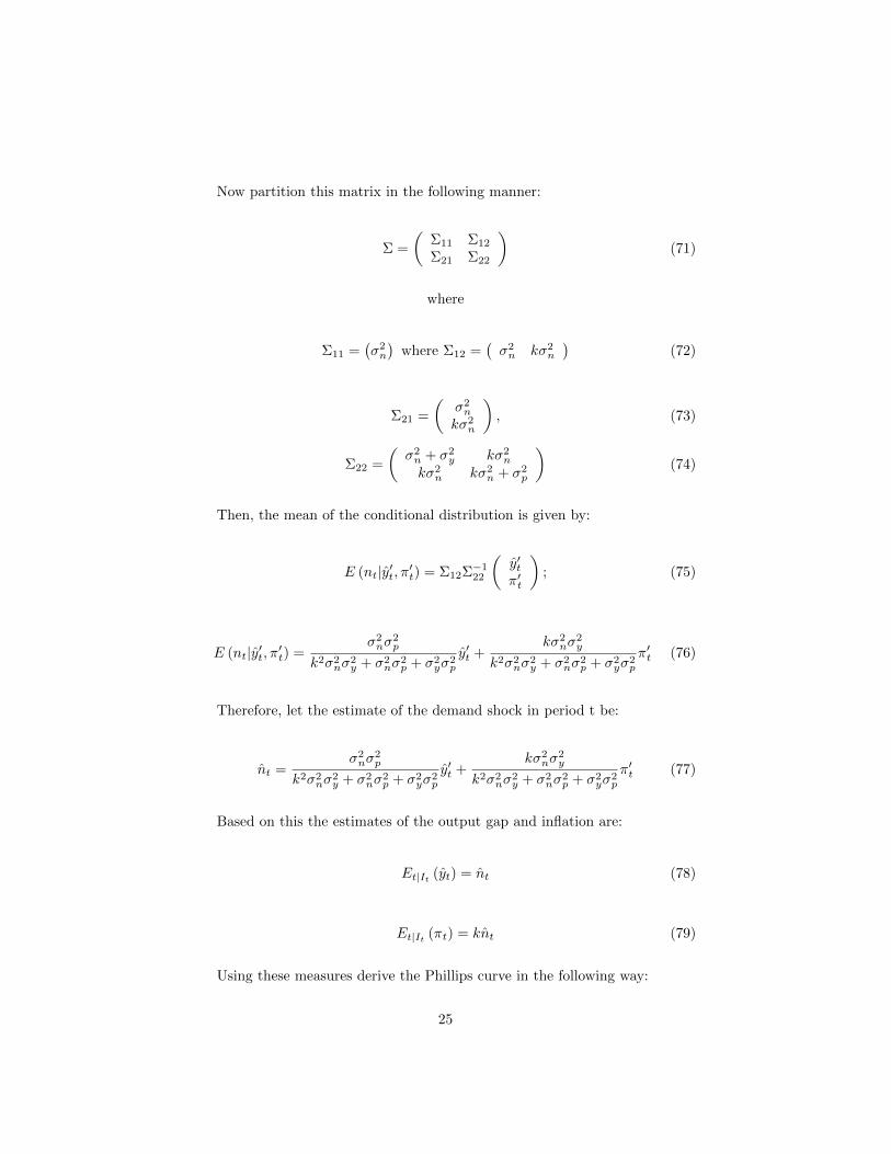
Now partition this matrix in the following manner:

Σ =

(Σ11 Σ12

Σ21 Σ22

)(71)

where

Σ11 =(σ2n

)where Σ12 =

(σ2n kσ2

n

)(72)

Σ21 =

(σ2n

kσ2n

), (73)

Σ22 =

(σ2n + σ2

y kσ2n

kσ2n kσ2

n + σ2p

)(74)

Then, the mean of the conditional distribution is given by:

E (nt|y′t, π′t) = Σ12Σ−122

(y′tπ′t

); (75)

E (nt|y′t, π′t) =σ2nσ

2p

k2σ2nσ

2y + σ2

nσ2p + σ2

yσ2p

y′t +kσ2

nσ2y

k2σ2nσ

2y + σ2

nσ2p + σ2

yσ2p

π′t (76)

Therefore, let the estimate of the demand shock in period t be:

nt =σ2nσ

2p

k2σ2nσ

2y + σ2

nσ2p + σ2

yσ2p

y′t +kσ2

nσ2y

k2σ2nσ

2y + σ2

nσ2p + σ2

yσ2p

π′t (77)

Based on this the estimates of the output gap and inflation are:

Et|It (yt) = nt (78)

Et|It (πt) = knt (79)

Using these measures derive the Phillips curve in the following way:

25

p∗t = (1− αβ)Et|Itpt + (1− αβ) (δ + γ − 1)Et|It yt +αβEt|Itpt+1 +αβEt|Itqt+1

(80)

subtracting pt from both sides yields:

qt = (1− αβ) (δ + γ − 1)Et|It yt + αβEt|Itpt+1 + αβEt|Itqt+1 (81)

Now, use the expectations derived previously:

qt = (1 − αβ) (δ + γ − 1)Et|It

σ2nσ2p

k2σ2nσ2y + σ2nσ

2p + σ2yσ

2p

y′t +

kσ2nσ2y

k2σ2nσ2y + σ2nσ

2p + σ2yσ

2p

π′t

+αβEt|Itpt+1+αβEt|It qt+1

(82)

Now expand the term in square brackets:

qt = (1 − αβ) (δ + γ − 1)Et|It

σ2nσ2p

k2σ2nσ2y + σ2nσ

2p + σ2yσ

2p

yt +kσ2nσ

2y

k2σ2nσ2y + σ2nσ

2p + σ2yσ

2p

πt

(83)

+

σ2nσ2p

k2σ2nσ2y+σ2nσ

2p+σ

2yσ

2pωt +

kσ2nσ2y

k2σ2nσ2y+σ2nσ

2p+σ

2yσ

2pεt

+ αβEt|Itpt+1 + αβEt|It qt+1

Therefore, use the initial condition that πt = kyt, to give the followingexpression:

qt = (1 − αβ) (δ + γ − 1)Et|It

σ2nσ2p

k2σ2nσ2y+σ2nσ

2p+σ

2yσ

2p

+k2σ2nσ

2y

k2σ2nσ2y+σ2nσ

2p+σ

2yσ

2p

yt+

+

σ2nσ2p

k2σ2nσ2y+σ2nσ

2p+σ

2yσ

2pωt +

kσ2nσ2y

k2σ2nσ2y+σ2nσ

2p+σ

2yσ

2pεt

+ αβEt|Itpt+1 + αβEt|It qt+1

This leads to a Phillips Curve with the following form:

πt =(1 − α) (1 − αβ) (δ + γ − 1)

α

σ2nσ2p

k2σ2nσ2y + σ2nσ

2p + σ2yσ

2p

+k2σ2nσ

2y

k2σ2nσ2y + σ2nσ

2p + σ2yσ

2p

yt+ (84)

+ 1−αα

σ2nσ2p

k2σ2nσ2y+σ2nσ

2p+σ

2yσ

2pωt +

kσ2nσ2y

k2σ2nσ2y+σ2nσ

2p+σ

2yσ

2pεt

+ βEt|Itπt+1

The terms in curved brackets are the terms which describe the noise errorswhich cause inflation to fluctuate away from the steady state equilibrium. Thefull solution is obtained numerically by finding the root of the equation, whichguarantees consistency between the relationship between inflation and outputthat is postulated at the beginning of this section:

26

(1 − α) (1 − αβ) (δ + γ − 1)

α

σ2nσ2p

k2σ2nσ2y + σ2nσ

2p + σ2yσ

2p

+k2σ2nσ

2y

k2σ2nσ2y + σ2nσ

2p + σ2yσ

2p

= k (85)

These solutions have been plotted for a variety of values of σ2p and σ2

y.I alsoassume a set of values for exogenous parameters as shown in the table below:

α β γ θ δ σ2η

0.75 1.04−14 1.5 7.88 0.6 0.03Y

These assumptions imply that the average mark-up per firm will be approx-imately 14%, and that the variance of the shocks to output is approximately3% of steady state output as denoted by Y. Furthermore, the assumptions onthe utility parameters are such that the discount rate is 4% per annum andthe inter-temporal elasticity of substitution is -1.67, while the assumption onγ corresponds to a labour supply elasticity of 1

γ−1 , here is equal to 2. The as-sumption that α is set to 0.75, corresponds to an average length of a contract of4 periods, hence if this model is taken to quarterly data, this implies an averagelength of price setting of 1 year.

As the solution is plotted for a set of noise levels, some results are immedi-ately apparent. Firstly, along the axes (where either σ2

p or σ2y equal zero) the

solution just reduces to the standard Phillips curve that had been solved for

27

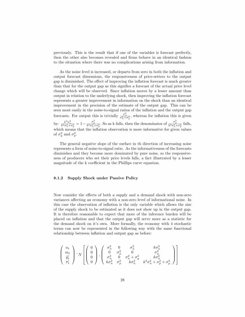
previously. This is the result that if one of the variables is forecast perfectly,then the other also becomes revealed and firms behave in an identical fashionto the situation where there was no complications arising from information.

As the noise level is increased, or departs from zero in both the inflation andoutput forecast dimensions, the responsiveness of price-setters to the outputgap is diminished. The effect of improving the inflation forecast is much greaterthan that for the output gap as this signifies a forecast of the actual price levelchange which will be observed. Since inflation moves by a lesser amount thanoutput in relation to the underlying shock, then improving the inflation forecastrepresents a greater improvement in information on the shock than an identicalimprovement in the precision of the estimate of the output gap. This can beseen most easily in the noise-to-signal ratios of the inflation and the output gap

forecasts. For output this is triviallyσ2n

σ2n+σ

2y, whereas for inflation this is given

by:k2σ2

n

k2σ2n+σ

2p

= 1− σ2p

k2σ2n+σ

2p. So as k falls, then the denominator of

σ2p

k2σ2n+σ

2p

falls,

which means that the inflation observation is more informative for given valuesof σ2

y and σ2p.

The general negative slope of the surface in th direction of increasing noiserepresents a form of noise-to-signal ratio. As the informativeness of the forecastsdiminishes and they become more dominated by pure noise, so the responsive-ness of producers who set their price levels falls, a fact illustrated by a lessermagnitude of the k coefficient in the Phillips curve equation.

8.1.2 Supply Shock under Passive Policy

Now consider the effects of both a supply and a demand shock with non-zerovariances affecting an economy with a non-zero level of informational noise. Inthis case the observation of inflation is the only variable which allows the sizeof the supply shock to be estimated as it does not show up in the output gap.It is therefore reasonable to expect that more of the inference burden will beplaced on inflation and that the output gap will serve more as a statistic forthe demand shock on it’s own. More formally, the economy with 4 stochasticterms can now be represented in the following way with the same functionalrelationship between inflation and output gap as before:

ntmt

y′tπ′t

˜N

0000

,

σ2n 0 σ2

n kσ2n

0 σ2µ 0 σ2

µ

σ2n 0 σ2

n + σ2y kσ2

n

kσ2n σ2

µ kσ2n k2σ2

n + σ2p + σ2

µ

28

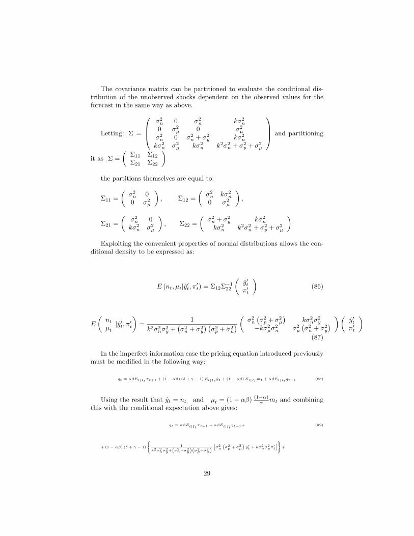
The covariance matrix can be partitioned to evaluate the conditional dis-tribution of the unobserved shocks dependent on the observed values for theforecast in the same way as above.

Letting: Σ =

σ2n 0 σ2

n kσ2n

0 σ2µ 0 σ2

µ

σ2n 0 σ2

n + σ2y kσ2

n

kσ2n σ2

µ kσ2n k2σ2

n + σ2p + σ2

µ

and partitioning

it as Σ =

(Σ11 Σ12

Σ21 Σ22

)the partitions themselves are equal to:

Σ11 =

(σ2n 0

0 σ2µ

), Σ12 =

(σ2n kσ2

n

0 σ2µ

),

Σ21 =

(σ2n 0

kσ2n σ2

µ

), Σ22 =

(σ2n + σ2

y kσ2n

kσ2n k2σ2

n + σ2p + σ2

µ

)Exploiting the convenient properties of normal distributions allows the con-

ditional density to be expressed as:

E (nt, µt|y′t, π′t) = Σ12Σ−122

(y′tπ′t

)(86)

E

(ntµt|y′t, π′t

)=

1

k2σ2nσ

2y +

(σ2n + σ2

y

) (σ2p + σ2

µ

) ( σ2n

(σ2p + σ2

µ

)kσ2

nσ2y

−kσ2µσ

2n σ2

µ

(σ2n + σ2

y

) )( y′tπ′t

)(87)

In the imperfect information case the pricing equation introduced previouslymust be modified in the following way:

qt = αβEt|Itπt+1 + (1 − αβ) (δ + γ − 1)Et|It yt + (1 − αβ)Et|Itmt + αβEt|It qt+1 (88)

Using the result that yt = nt, and µt = (1− αβ) (1−α)α mt and combining

this with the conditional expectation above gives:

qt = αβEt|Itπt+1 + αβEt|It qt+1+ (89)

+ (1 − αβ) (δ + γ − 1)

1

k2σ2nσ2y+

(σ2n+σ2y

)(σ2p+σ

2µ

) [σ2n (σ2p + σ2µ

)y′t + kσ2nσ

2yπ′t

]+

29

+ (1 − αβ)

((1 − αβ) (1−α)

α

)−11

k2σ2nσ2y+

(σ2n+σ2y

)(σ2p+σ

2µ

) [σ2µ (σ2n + σ2y

)π′t − kσ

2µσ

2ny′t

]

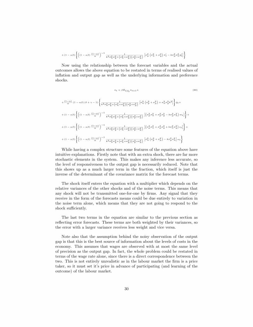
Now using the relationship between the forecast variables and the actualoutcomes allows the above equation to be restated in terms of realised values ofinflation and output gap as well as the underlying information and preferenceshocks.

πt = βEt|Itπt+1+ (90)

+(1−α)α

(1 − αβ) (δ + γ − 1)

1

k2σ2nσ2y+

(σ2n+σ2y

)(σ2p+σ

2µ

) [σ2n (σ2p + σ2µ

)+ σ2nσ

2yk

2] yt+

+ (1 − αβ)

((1 − αβ) (1−α)

α

)−11

k2σ2nσ2y+

(σ2n+σ2y

)(σ2p+σ

2µ

) [(σ2µσ2n + σ2µσ2y − kσ

2µσ

2n

)mt

]+

+ (1 − αβ)

((1 − αβ) (1−α)

α

)−11

k2σ2nσ2y+

(σ2n+σ2y

)(σ2p+σ

2µ

) [(σ2µσ2n + σ2µσ2y + kσ2nσ

2y

)εt

]+

+ (1 − αβ)

((1 − αβ) (1−α)

α

)−11

k2σ2nσ2y+

(σ2n+σ2y

)(σ2p+σ

2µ

) [σ2n (σ2p + σ2µ

)− kσ2µσ

2n

]ωt

While having a complex structure some features of the equation above haveintuitive explanations. Firstly note that with an extra shock, there are far morestochastic elements in the system. This makes any inference less accurate, sothe level of responsiveness to the output gap is necessarily reduced. Note thatthis shows up as a much larger term in the fraction, which itself is just theinverse of the determinant of the covariance matrix for the forecast terms.

The shock itself enters the equation with a multiplier which depends on therelative variances of the other shocks and of the noise terms. This means thatany shock will not be transmitted one-for-one by firms. Any signal that theyreceive in the form of the forecasts means could be due entirely to variation inthe noise term alone, which means that they are not going to respond to theshock sufficiently.

The last two terms in the equation are similar to the previous section asreflecting error forecasts. These terms are both weighted by their variances, sothe error with a larger variance receives less weight and vice versa.

Note also that the assumption behind the noisy observation of the outputgap is that this is the best source of information about the levels of costs in theeconomy. This assumes that wages are observed with at most the same levelof precision as the output gap. In fact, the whole problem could be restated interms of the wage rate alone, since there is a direct correspondence between thetwo. This is not entirely unrealistic as in the labour market the firm is a pricetaker, so it must set it’s price in advance of participating (and learning of theoutcome) of the labour market.

30

8.2 Active Central Bank Policy

8.2.1 Demand Shock

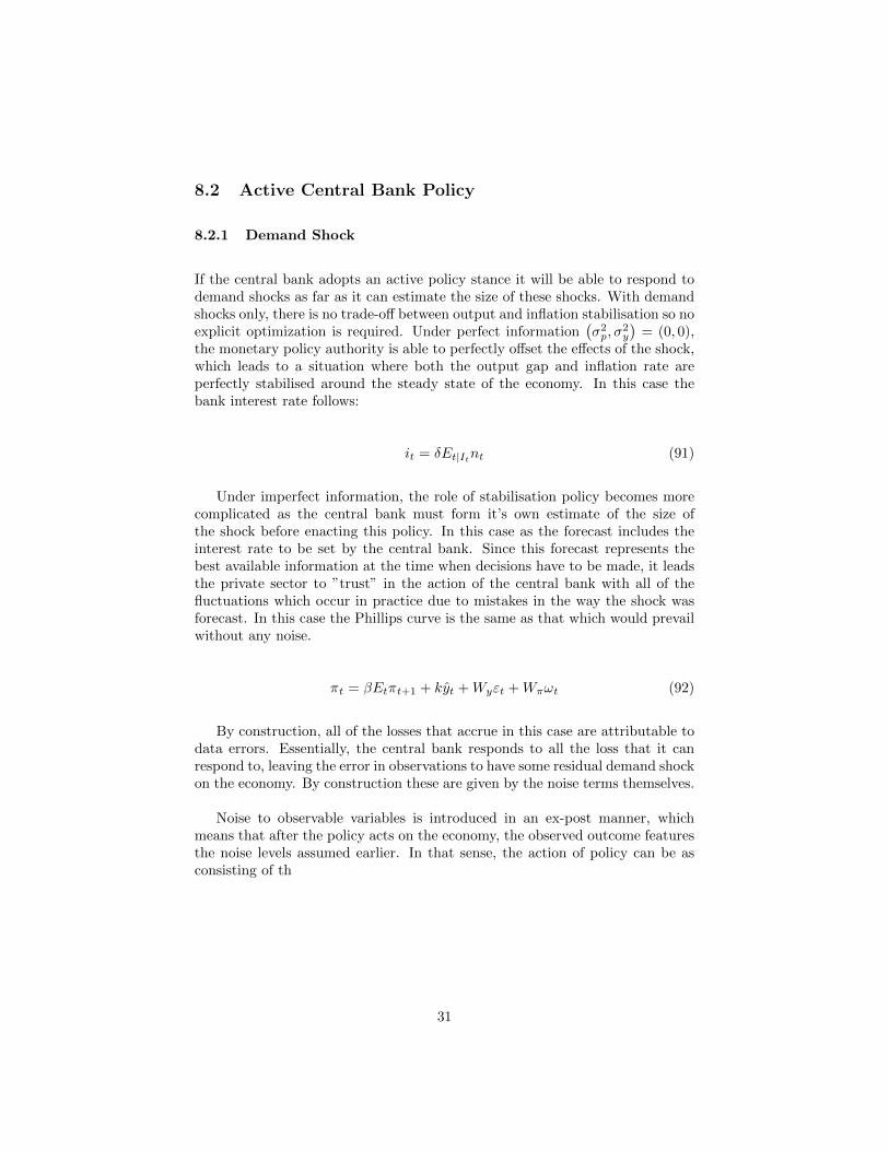
If the central bank adopts an active policy stance it will be able to respond todemand shocks as far as it can estimate the size of these shocks. With demandshocks only, there is no trade-off between output and inflation stabilisation so noexplicit optimization is required. Under perfect information

(σ2p, σ

2y

)= (0, 0),

the monetary policy authority is able to perfectly offset the effects of the shock,which leads to a situation where both the output gap and inflation rate areperfectly stabilised around the steady state of the economy. In this case thebank interest rate follows:

it = δEt|Itnt (91)

Under imperfect information, the role of stabilisation policy becomes morecomplicated as the central bank must form it’s own estimate of the size ofthe shock before enacting this policy. In this case as the forecast includes theinterest rate to be set by the central bank. Since this forecast represents thebest available information at the time when decisions have to be made, it leadsthe private sector to ”trust” in the action of the central bank with all of thefluctuations which occur in practice due to mistakes in the way the shock wasforecast. In this case the Phillips curve is the same as that which would prevailwithout any noise.

πt = βEtπt+1 + kyt +Wyεt +Wπωt (92)

By construction, all of the losses that accrue in this case are attributable todata errors. Essentially, the central bank responds to all the loss that it canrespond to, leaving the error in observations to have some residual demand shockon the economy. By construction these are given by the noise terms themselves.

Noise to observable variables is introduced in an ex-post manner, whichmeans that after the policy acts on the economy, the observed outcome featuresthe noise levels assumed earlier. In that sense, the action of policy can be asconsisting of th

31

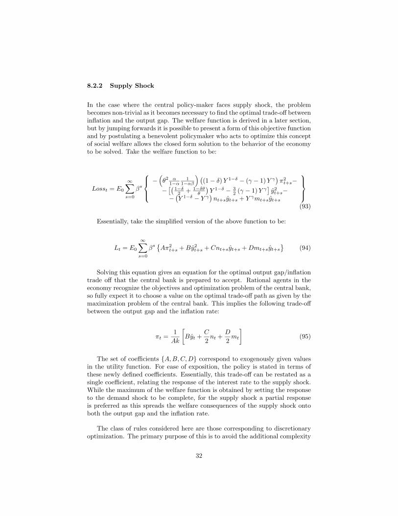
8.2.2 Supply Shock

In the case where the central policy-maker faces supply shock, the problembecomes non-trivial as it becomes necessary to find the optimal trade-off betweeninflation and the output gap. The welfare function is derived in a later section,but by jumping forwards it is possible to present a form of this objective functionand by postulating a benevolent policymaker who acts to optimize this conceptof social welfare allows the closed form solution to the behavior of the economyto be solved. Take the welfare function to be:

Losst = E0

∞∑s=0

βs

−(θ2 α

1−α1

1−αβ

) ((1− δ)Y 1−δ − (γ − 1)Y γ

)π2t+s−

−[(

1−δ2 + 1−δθ

θ

)Y 1−δ − 3

2 (γ − 1)Y γ]y2t+s−

−(Y 1−δ − Y γ

)nt+syt+s + Y γmt+syt+s

(93)

Essentially, take the simplified version of the above function to be:

Lt = E0

∞∑s=0

βsAπ2

t+s +By2t+s + Cnt+syt+s +Dmt+syt+s

(94)

Solving this equation gives an equation for the optimal output gap/inflationtrade off that the central bank is prepared to accept. Rational agents in theeconomy recognize the objectives and optimization problem of the central bank,so fully expect it to choose a value on the optimal trade-off path as given by themaximization problem of the central bank. This implies the following trade-offbetween the output gap and the inflation rate:

πt =1

Ak

[Byt +

C

2nt +

D

2mt

](95)

The set of coefficients A,B,C,D correspond to exogenously given valuesin the utility function. For ease of exposition, the policy is stated in terms ofthese newly defined coefficients. Essentially, this trade-off can be restated as asingle coefficient, relating the response of the interest rate to the supply shock.While the maximum of the welfare function is obtained by setting the responseto the demand shock to be complete, for the supply shock a partial responseis preferred as this spreads the welfare consequences of the supply shock ontoboth the output gap and the inflation rate.

The class of rules considered here are those corresponding to discretionaryoptimization. The primary purpose of this is to avoid the additional complexity

32

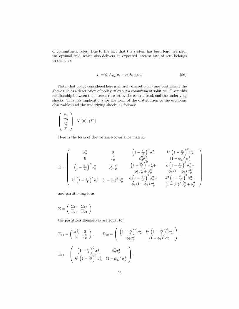
of commitment rules. Due to the fact that the system has been log-linearized,the optimal rule, which also delivers an expected interest rate of zero belongsto the class:

it = φ1Et|Itnt + φ2Et|Itmt (96)

Note, that policy considered here is entirely discretionary and postulating theabove rule as a description of policy rules out a commitment solution. Given thisrelationship between the interest rate set by the central bank and the underlyingshocks. This has implications for the form of the distribution of the economicobservables and the underlying shocks as follows:

ntmt

y′tπ′t

˜N [(0) , (Σ)]

Here is the form of the variance-covariance matrix:

Σ =

σ2n 0

(1− φ1

δ

)2σ2n k2

(1− φ1

δ

)2σ2n

0 σ2µ φ22σ

2µ (1− φ2)

2σ2µ(

1− φ1

δ

)2σ2n φ22σ

2µ

(1− φ1

δ

)2σ2n+

φ22σ2µ + σ2

y

k(

1− φ1

δ

)2σ2n+

φ2 (1− φ2)σ2µ

k2(

1− φ1

δ

)2σ2n (1− φ2)

2σ2µ

k(

1− φ1

δ

)2σ2n+

φ2 (1− φ2)σ2µ

k2(

1− φ1

δ

)2σ2n+

(1− φ2)2σ2µ + σ2

p

and partitioning it as

Σ =

(Σ11 Σ12

Σ21 Σ22

)the partitions themselves are equal to:

Σ11 =

(σ2n 0

0 σ2µ

), Σ12 =

(1− φ1

δ

)2σ2n k2

(1− φ1

δ

)2σ2n

φ22σ2µ (1− φ2)

2σ2µ

,

Σ21 =

(

1− φ1

δ

)2σ2n φ22σ

2µ

k2(

1− φ1

δ

)2σ2n (1− φ2)

2σ2µ

,

33

Σ22 =

(

1− φ1

δ

)2σ2n+

φ22σ2µ + σ2

y

k(

1− φ1

δ

)2σ2n+

φ2 (1− φ2)σ2µ

k(

1− φ1

δ

)2σ2n+

φ2 (1− φ2)σ2µ

k2(

1− φ1

δ

)2σ2n+

(1− φ2)2σ2µ + σ2

p

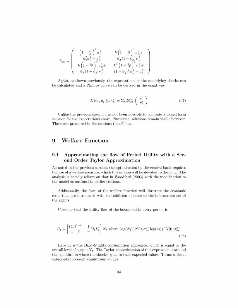
Again, as shown previously, the expectations of the underlying shocks can

be calculated and a Phillips curve can be derived in the usual way.

E (nt, µt|y′t, π′t) = Σ12Σ−122

(y′tπ′t

)(97)

Unlike the previous case, it has not been possible to compute a closed formsolution for the expectations above. Numerical solutions remain viable however.These are presented in the sections that follow.

9 Welfare Function

9.1 Approximating the flow of Period Utility with a Sec-ond Order Taylor Approximation

As noted in the previous section, the optimisation by the central bank requiresthe use of a welfare measure, which this section will be devoted to deriving. Theanalysis is heavily reliant on that in Woodford (2003) with the modification tothe model as outlined in earlier sections.

Additionally, the form of the welfare function will illustrate the economiccosts that are introduced with the addition of noise to the information set ofthe agents.

Consider that the utility flow of the household in every period is:

Ut =

[(Ct)

1−δ

1− δ− 1

γMtL

γt

]Nt where log(Nt)˜N(0, σ2

n) log(Mt)˜N(0, σ2m)

(98)

Here Ct is the Dixit-Stiglitz consumption aggregate, which is equal to theoverall level of output Yt. The Taylor approximation of this expression is aroundthe equilibrium where the shocks equal to their expected values. Terms withoutsubscripts represent equilibrium values.

34

Ut =

(Y 1+δ

1 + δ− 1

γY γ)

+ (99)

+(Y 1−δ

1−δ −1γMY γ

)(Nt −N)− 1

γYγ (Mt −M) +

+[Y −δ − Y γ−1

] ∫ 1

0Yt (i)− Y (i) di− Y γ−1 (Nt −N) (Mt −M) +

+ 12

[−δY −δ−1 − (γ − 1)Y γ−2

] ∫ 1

0(Yt (i)− Y (i))

2di+

+[1−δθθ Y −1−δ − (γ − 1)Y γ−2

] ∫ 1

0Yt (i)− Y (i)

∫ 1

0Yt (j)− Y (j) djdi+

+(Y −δ − Y γ−1

)(Nt −N)

∫ 1

0Yt (i)− Y (i) di−

−Y γ−1 (Mt −M)∫ 1

0Yt (i)− Y (i) di+O

(|Yt (i) , Nt,Mt|3

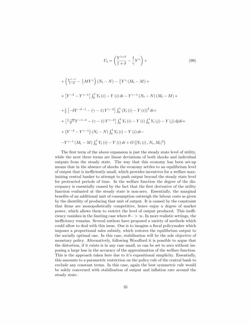
)The first term of the above expansion is just the steady state level of utility,

while the next three terms are linear deviations of both shocks and individualoutputs from the steady state. The way that this economy has been set-upmeans that in the absence of shocks the economy settles to an equilibrium levelof output that is inefficiently small, which provides incentives for a welfare max-imizing central banker to attempt to push output beyond the steady state levelfor protracted periods of time. In the welfare function the degree of the dis-crepancy is essentially caused by the fact that the first derivative of the utilityfunction evaluated at the steady state is non-zero. Essentially, the marginalbenefits of an additional unit of consumption outweigh the labour costs as givenby the disutility of producing that unit of output. It is caused by the constraintthat firms are monopolistically competitive, hence enjoy a degree of marketpower, which allows them to restrict the level of output produced. This ineffi-ciency vanishes in the limiting case where θ− >∞. In more realistic settings, theinefficiency remains. Several authors have proposed a variety of methods whichcould allow to deal with this issue. One is to imagine a fiscal policymaker whichimposes a proportional sales subsidy, which restores the equilibrium output tothe socially optimal one. In this case, stabilisation will be the sole objective ofmonetary policy. Alternatively, following Woodford it is possible to argue thatthe distortion, if it exists is in any case small, so can be set to zero without im-posing a large loss in the accuracy of the approximation of the welfare function.This is the approach taken here due to it’s expositional simplicity. Essentially,this amounts to a parametric restriction on the policy rule of the central bank toexclude any constant terms. In this case, again the best symmetric rule wouldbe solely concerned with stabilisation of output and inflation rate around thesteady state.

35

The second term on the third line is the interaction term between the twosources of shock, which in expectation will be zero due to the assumption ofindependence between the supply shock (Mt) and the demand shock (Nt). Thequadratic term in the individual outputs of the firms is a measure of the dis-persion of individual outputs from their steady state values. As this is causedby the formation of atoms of firms which are unable to change their prices ev-ery period leading to asymmetries in the production of different goods. Due tosymmetry the most efficient production plan involves all the firms producingidentical quantities equalised at marginal costs. Due to nominal frictions theasymmetry in the production of firms causes a reduction in welfare. The termon the fourth line of the above equation refers to the covariance between onefirm’s output with that of all the others. Since the firms in this economy areall directly competing against all the others so this term is non-zero as anyadjustment by one firm will cause the outputs of others to change. The termson lines 5 and 6 are simply the covariance between the level of production andthe effect of the shocks. These terms similarly have a non-negligible effect onwelfare as the level of output has already been shown to depend directly on themagnitude of shocks, so these are not independent from the each other.

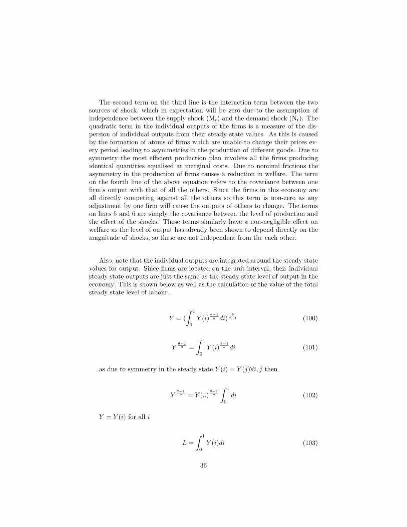
Also, note that the individual outputs are integrated around the steady statevalues for output. Since firms are located on the unit interval, their individualsteady state outputs are just the same as the steady state level of output in theeconomy. This is shown below as well as the calculation of the value of the totalsteady state level of labour.

Y = (

∫ 1

0

Y (i)θ−1θ di)

θθ−1 (100)

Yθ−1θ =

∫ 1

0

Y (i)θ−1θ di (101)

as due to symmetry in the steady state Y (i) = Y (j)∀i, j then

Yθ−1θ = Y (..)

θ−1θ

∫ 1

0

di (102)

Y = Y (i) for all i

L =

∫ 1

0

Y (i)di (103)

36

L = Y

∫ 1

0

di (104)

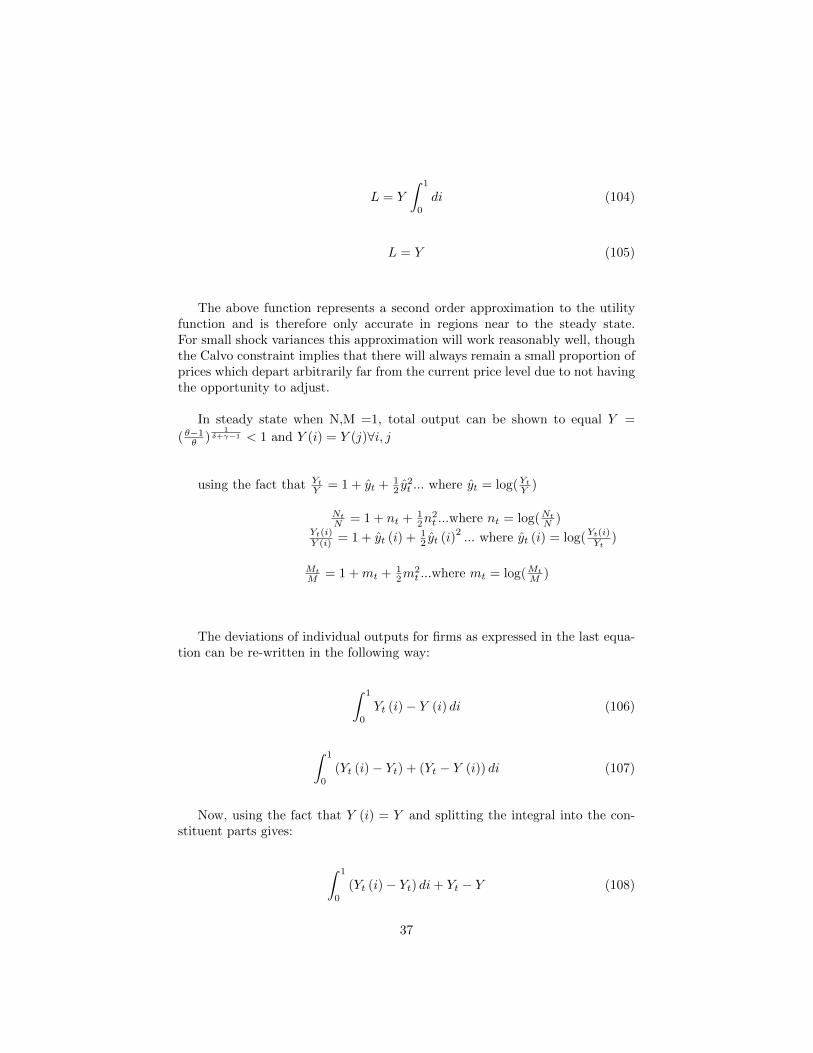
L = Y (105)

The above function represents a second order approximation to the utilityfunction and is therefore only accurate in regions near to the steady state.For small shock variances this approximation will work reasonably well, thoughthe Calvo constraint implies that there will always remain a small proportion ofprices which depart arbitrarily far from the current price level due to not havingthe opportunity to adjust.

In steady state when N,M =1, total output can be shown to equal Y =

( θ−1θ )1

δ+γ−1 < 1 and Y (i) = Y (j)∀i, j

using the fact that YtY = 1 + yt + 1

2 y2t ... where yt = log(YtY )

NtN = 1 + nt + 1

2n2t ...where nt = log(NtN )

Yt(i)Y (i) = 1 + yt (i) + 1

2 yt (i)2... where yt (i) = log(Yt(i)Yt

)

Mt

M = 1 +mt + 12m

2t ...where mt = log(Mt

M )

The deviations of individual outputs for firms as expressed in the last equa-tion can be re-written in the following way:

∫ 1

0

Yt (i)− Y (i) di (106)

∫ 1

0

(Yt (i)− Yt) + (Yt − Y (i)) di (107)

Now, using the fact that Y (i) = Y and splitting the integral into the con-stituent parts gives:

∫ 1

0

(Yt (i)− Yt) di+ Yt − Y (108)

37

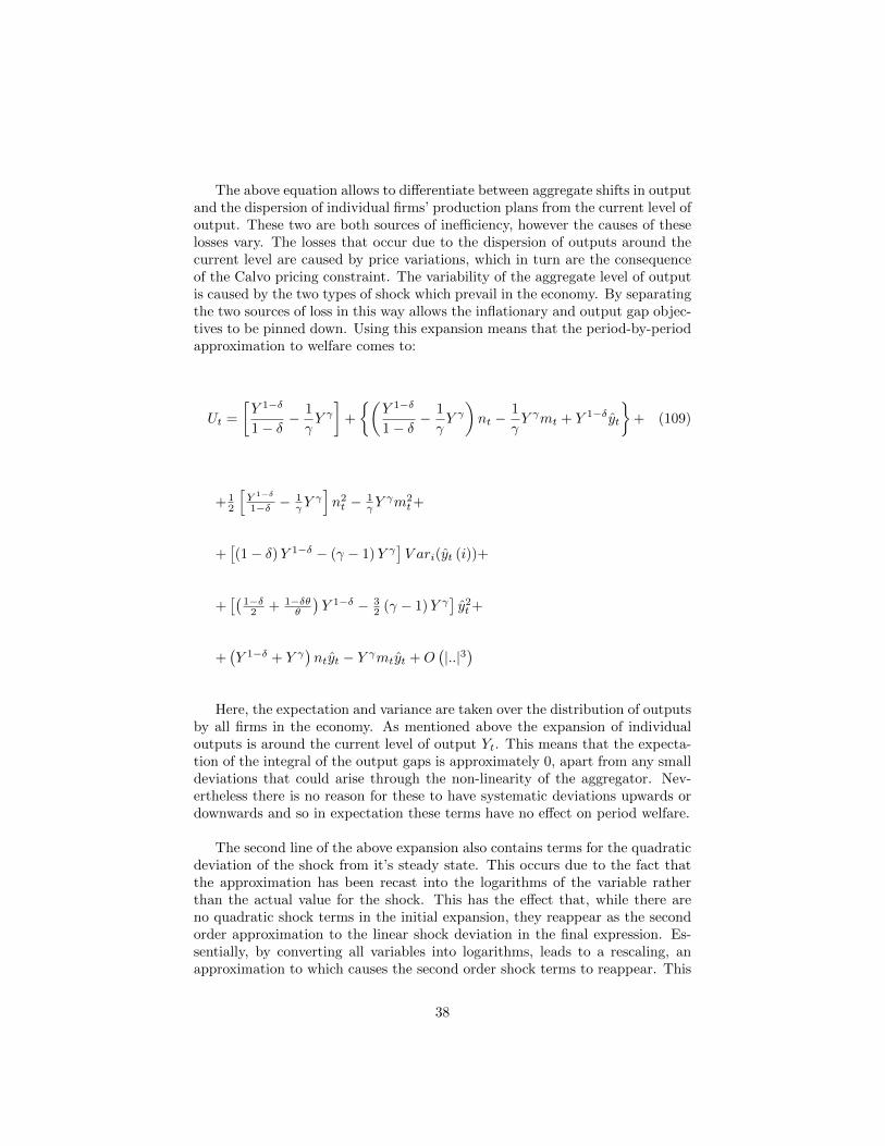
The above equation allows to differentiate between aggregate shifts in outputand the dispersion of individual firms’ production plans from the current level ofoutput. These two are both sources of inefficiency, however the causes of theselosses vary. The losses that occur due to the dispersion of outputs around thecurrent level are caused by price variations, which in turn are the consequenceof the Calvo pricing constraint. The variability of the aggregate level of outputis caused by the two types of shock which prevail in the economy. By separatingthe two sources of loss in this way allows the inflationary and output gap objec-tives to be pinned down. Using this expansion means that the period-by-periodapproximation to welfare comes to:

Ut =

[Y 1−δ

1− δ− 1

γY γ]

+

(Y 1−δ

1− δ− 1

γY γ)nt −

1

γY γmt + Y 1−δ yt

+ (109)

+ 12

[Y 1−δ

1−δ −1γY

γ]n2t − 1

γYγm2

t+

+[(1− δ)Y 1−δ − (γ − 1)Y γ

]V ari(yt (i))+

+[(

1−δ2 + 1−δθ

θ

)Y 1−δ − 3

2 (γ − 1)Y γ]y2t+

+(Y 1−δ + Y γ

)ntyt − Y γmtyt +O

(|..|3)

Here, the expectation and variance are taken over the distribution of outputsby all firms in the economy. As mentioned above the expansion of individualoutputs is around the current level of output Yt. This means that the expecta-tion of the integral of the output gaps is approximately 0, apart from any smalldeviations that could arise through the non-linearity of the aggregator. Nev-ertheless there is no reason for these to have systematic deviations upwards ordownwards and so in expectation these terms have no effect on period welfare.

The second line of the above expansion also contains terms for the quadraticdeviation of the shock from it’s steady state. This occurs due to the fact thatthe approximation has been recast into the logarithms of the variable ratherthan the actual value for the shock. This has the effect that, while there areno quadratic shock terms in the initial expansion, they reappear as the secondorder approximation to the linear shock deviation in the final expression. Es-sentially, by converting all variables into logarithms, leads to a rescaling, anapproximation to which causes the second order shock terms to reappear. This

38

is also true for all other variables, although as they all have non-zero secondderivatives, the effect of the logarithmic expansion is to supplement the coeffi-cients in the welfare function. Alternative cases can now be analysed as the lossfunction at time t is given by:

Losst = Et

∞∑s=0

βsUt+s (110)

This means that the loss function can be rewritten more completely as:

Losst = Et

∞∑s=0

βs

[(1− δ)Y 1−δ − (γ − 1)Y γ

]V ari(yt (i))+

+[(

1−δ2 + 1−δθ

θ

)Y 1−δ − 3

2 (γ − 1)Y γ]y2t+

+(Y 1−δ + Y γ

)ntyt − Y γmtyt+

+t.i.s.+O(|..|3)

(111)

Here t.i.s. refers to terms which are independent of the structure of theeconomy (in the sense of the levels of noise in relation to the actual shocks) aswell as any policy actions. These contain the quadratic shock deviations as wellas the constant welfare level in addition to the linear terms.

The above expression for the welfare losses based on the representative con-sumer utility function shows that the terms relevant to changing the structureof the economy will be those which are non-constant as the informational regimeis adjusted. Therefore, the function above can be adjusted to give the following:

Losst = Et

∞∑t=0

βs

[(1− δ)Y 1−δ − (γ − 1)Y γ

]V ari(yt (i))+

+[(

1−δ2 + 1−δθ

θ

)Y 1−δ − 3

2 (γ − 1)Y γ]y2t+

+(Y 1−δ + Y γ

)ntyt − Y γmtyt+

+t.i.s.+O(|..|3)

(112)

Essentially, the terms that matter for welfare evaluation are the varianceof aggregate output and the variance of output between firms in the economy,which is determined by the degree of price dispersion. As the demand curvegiven by Dixit-Stiglitz preferences is:

log Yt(i) = log Yt − θ(logPt(i)− logPt) (113)

39

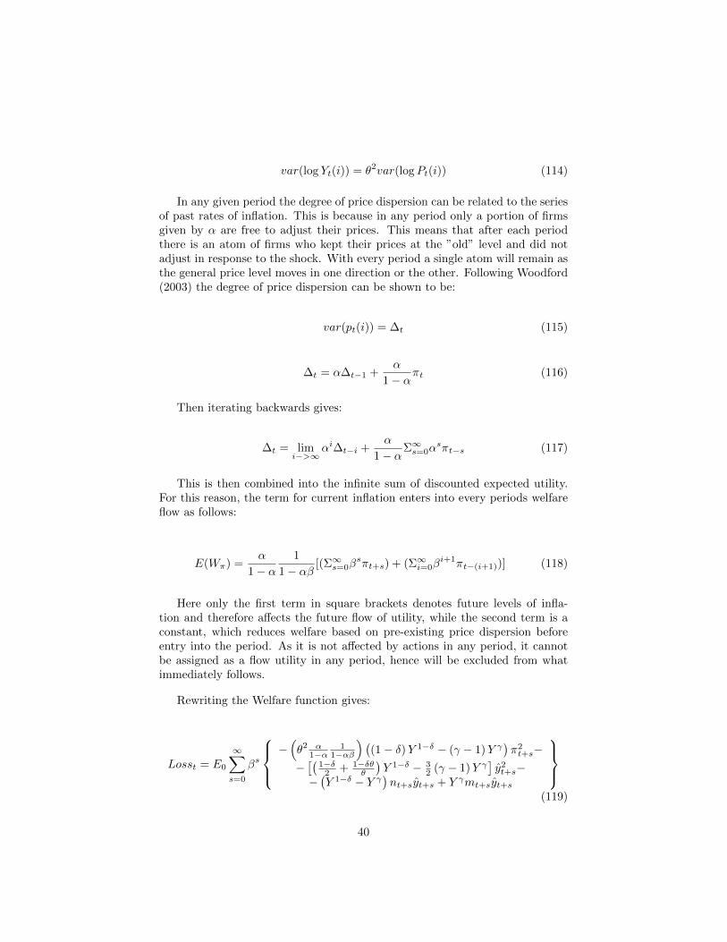
var(log Yt(i)) = θ2var(logPt(i)) (114)

In any given period the degree of price dispersion can be related to the seriesof past rates of inflation. This is because in any period only a portion of firmsgiven by α are free to adjust their prices. This means that after each periodthere is an atom of firms who kept their prices at the ”old” level and did notadjust in response to the shock. With every period a single atom will remain asthe general price level moves in one direction or the other. Following Woodford(2003) the degree of price dispersion can be shown to be:

var(pt(i)) = ∆t (115)

∆t = α∆t−1 +α

1− απt (116)

Then iterating backwards gives:

∆t = limi−>∞

αi∆t−i +α

1− αΣ∞s=0α

sπt−s (117)

This is then combined into the infinite sum of discounted expected utility.For this reason, the term for current inflation enters into every periods welfareflow as follows:

E(Wπ) =α

1− α1

1− αβ[(Σ∞s=0β

sπt+s) + (Σ∞i=0βi+1πt−(i+1))] (118)

Here only the first term in square brackets denotes future levels of infla-tion and therefore affects the future flow of utility, while the second term is aconstant, which reduces welfare based on pre-existing price dispersion beforeentry into the period. As it is not affected by actions in any period, it cannotbe assigned as a flow utility in any period, hence will be excluded from whatimmediately follows.

Rewriting the Welfare function gives:

Losst = E0

∞∑s=0

βs

−(θ2 α

1−α1

1−αβ

) ((1− δ)Y 1−δ − (γ − 1)Y γ

)π2t+s−

−[(

1−δ2 + 1−δθ

θ

)Y 1−δ − 3

2 (γ − 1)Y γ]y2t+s−

−(Y 1−δ − Y γ

)nt+syt+s + Y γmt+syt+s

(119)

40

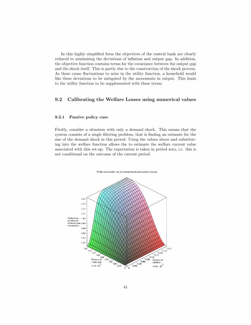
In this highly simplified form the objectives of the central bank are clearlyreduced to minimising the deviations of inflation and output gap. In addition,the objective function contains terms for the covariance between the output gapand the shock itself. This is partly due to the construction of the shock process.As these cause fluctuations to arise in the utility function, a household wouldlike these deviations to be mitigated by the movements in output. This leadsto the utility function to be supplemented with these terms.

9.2 Calibrating the Welfare Losses using numerical values

9.2.1 Passive policy case

Firstly, consider a situation with only a demand shock. This means that thesystem consists of a single filtering problem, that is finding an estimate for thesize of the demand shock in this period. Using the values above and substitut-ing into the welfare function allows the to estimate the welfare current valueassociated with this set-up. The expectation is taken in period zero, i.e. this isnot conditional on the outcome of the current period.

41

The above graph is plotted to show the percentage of steady state welfarethat the loss function takes under current settings for a variety of values of thenoise levels. Higher levels of noise correspond to a larger variance on the forecasterror terms and it is in terms of this variance that the results are shown. As canbe seen from the graph, as the levels of noise approach the magnitudes equivalentto the variance of the shock, then the cost in terms of steady state consumptionrises by approximately 0.2%. While on the scale of steady state welfare this mayappear to be an insignificant, this should be be seen as amplified by the scaleof the entire economy when compared to the costs of information gathering.

A broad feature of the result is that greater information uncertainty leadsto larger welfare losses. This is caused both by the fact that higher uncertaintyleads to lesser responsiveness to indicators since these are less informative. Fur-thermore, greater incidence of error lead to larger deviations from the efficientallocation due to the aggregation of decisions made on seeing errors in the fun-damental variables.

Moving along the axes of the graph, the losses from a lack of informationhave a similar shape, in fact they are almost identical, save for the fact thatalong the inflation axis, greater noise results in the inflation rates causes the losscurve to rise much more steeply along this axis and flattens out much earlierthan a similar interval along the axis of output noise. This means that for lowlevels of noise, at least, an improvement in inflation data would have a greatereffect on welfare than a similar one for the output gap. This is caused by thefact that as inflation only reacts to a demand shock through a response to thechange in the output gap, a greater precision in this variable has a more thanone for one effect on the precision of backing out the required output gap.

The above result can also be recomputed for the case where the economyis affected by both the demand and the supply shock as detailed in previoussections. Using the same values for exogenous variables as those used in theabove computation leads to the result as shown on the graph below.

42

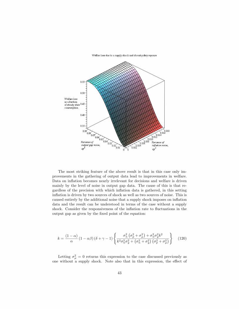
The most striking feature of the above result is that in this case only im-provements in the gathering of output data lead to improvements in welfare.Data on inflation becomes nearly irrelevant for decisions and welfare is drivenmainly by the level of noise in output gap data. The cause of this is that re-gardless of the precision with which inflation data is gathered, in this settinginflation is driven by two sources of shock as well as two sources of noise. This iscaused entirely by the additional noise that a supply shock imposes on inflationdata and the result can be understood in terms of the case without a supplyshock. Consider the responsiveness of the inflation rate to fluctuations in theoutput gap as given by the fixed point of the equation:

k =(1− α)

α(1− αβ) (δ + γ − 1)

σ2n

(σ2p + σ2

µ

)+ σ2

nσ2yk

2

k2σ2nσ

2y +

(σ2n + σ2

y

) (σ2p + σ2

µ

) (120)

Letting σ2µ = 0 returns this expression to the case discussed previously as

one without a supply shock. Note also that in this expression, the effect of

43

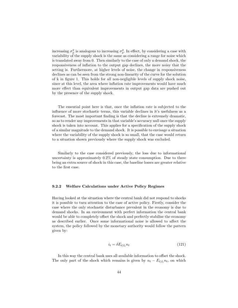
increasing σ2µ is analogous to increasing σ2

p. In effect, by considering a case withvariability of the supply shock is the same as considering a range for noise whichis translated away from 0. Then similarly to the case of only a demand shock, theresponsiveness of inflation to the output gap declines, the more noisy that thesetting is. Furthermore, at higher levels of noise, the change in responsivenessdeclines as can be seen from the strong non-linearity of the curve for the solutionof k in figure 1. This holds for all non-negligible levels of supply shock noise,since at this level, the area where inflation rate improvements would have muchmore effect than equivalent improvements in output gap data are pushed outby the presence of the supply shock.

The essential point here is that, once the inflation rate is subjected to theinfluence of more stochastic terms, this variable declines in it’s usefulness as aforecast. The most important finding is that the decline is extremely dramatic,so as to render any improvements in that variable’s accuracy null once the supplyshock is taken into account. This applies for a specification of the supply shockof a similar magnitude to the demand shock. It is possible to envisage a situationwhere the variability of the supply shock is so small, that the case would returnto a situation shown previously where the supply shock was excluded.

Similarly to the case considered previously, the loss due to informationaluncertainty is approximately 0.2% of steady state consumption. Due to therebeing an extra source of shock in this case, the baseline losses are greater relativeto the first case.

9.2.2 Welfare Calculations under Active Policy Regimes

Having looked at the situation where the central bank did not respond to shocksit is possible to turn attention to the case of active policy. Firstly, consider thecase where the only stochastic disturbance prevalent in the economy is due todemand shocks. In an environment with perfect information the central bankwould be able to completely offset the shock and perfectly stabilise the economyas described earlier. Once some informational noise is allowed to affect thesystem, the policy followed by the monetary authority would follow the patterngiven by:

it = δEt|Itnt (121)

In this way the central bank uses all available information to offset the shock.The only part of the shock which remains is given by nt − Et|Itnt, on which

44

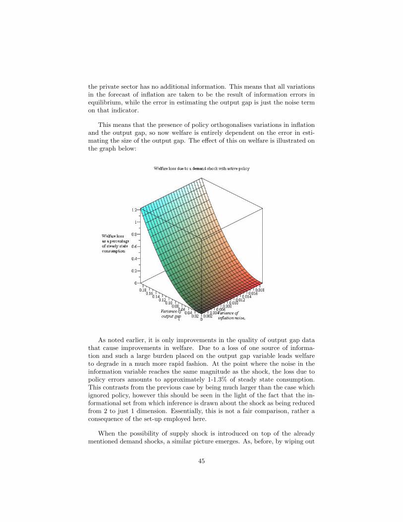
the private sector has no additional information. This means that all variationsin the forecast of inflation are taken to be the result of information errors inequilibrium, while the error in estimating the output gap is just the noise termon that indicator.

This means that the presence of policy orthogonalises variations in inflationand the output gap, so now welfare is entirely dependent on the error in esti-mating the size of the output gap. The effect of this on welfare is illustrated onthe graph below:

As noted earlier, it is only improvements in the quality of output gap datathat cause improvements in welfare. Due to a loss of one source of informa-tion and such a large burden placed on the output gap variable leads welfareto degrade in a much more rapid fashion. At the point where the noise in theinformation variable reaches the same magnitude as the shock, the loss due topolicy errors amounts to approximately 1-1.3% of steady state consumption.This contrasts from the previous case by being much larger than the case whichignored policy, however this should be seen in the light of the fact that the in-formational set from which inference is drawn about the shock as being reducedfrom 2 to just 1 dimension. Essentially, this is not a fair comparison, rather aconsequence of the set-up employed here.

When the possibility of supply shock is introduced on top of the alreadymentioned demand shocks, a similar picture emerges. As, before, by wiping out

45

the predictable shifts in the output gap, the presence of active policy orthog-onalises inflation and the output gap since there is no relevant information onthe output gap for the private sector once policy is taken into account.

The central bank sets interest rates according to the rule shown previously,i.e.

it = φ1Et|Itnt + φ2Et|Itmt (122)

The private sector takes this into account, which means that the value ofφ2 leads for a new relationship between the output gap and the inflation rate,this time led by the reaction function of the central bank. As before φ1 is setequal to δ to offset the predictable part of the demand shock completely, whileφ2 equals to a value prescribed by the welfare function as an optimal trade-offbetween inflation and the output gap. The effects on the loss function are shownin the graph below:

Broadly, the result is similar to the case immediately prior to this, notehowever that the loss function rises more quickly as noise levels increase due toan additional source of stochastic disturbances in the form of the supply shock.As before, the effect of policy is to orthogonalise the effect of the inflation rateand the output gap, hence it is only affected by errors in the output gap errors.

46

10 Conclusion

This thesis concentrated on the microfoundations of the effects of uncertaintyon agents in a standard DSGE economy. The results illustrate that noise byitself can act as a large burden on welfare in an economy where there are othersources of stochastic fluctuations. An immediate conclusion of this work isthat given imperfect information, observation errors will still have an effecton real variables. Furthermore, these fluctuations are not the result of anyunderlying shock. Essentially, these could be seen as another illustration of thepeso problem, shifts in real economic variables which have no basis in termsof shifts of the shock terms. A set describing the stochastic fluctuations ofthe economy must also take account of the informational shocks as well as thestochastic shocks which have a real effect on the rates of marginal utility.

The actual magnitude of the informational shocks is at most of the sameorder of magnitude as the shock itself, and smaller in most other cases. Thisis a consequence of the informational filtering which agents perform in thissetting, which acts in a similar fashion to the noise-to-signal ratio introducedby Lucas. In other words, the mechanism described here does not have a strongamplification property. In order to be able to explain large economic fluctuationsit becomes necessary to assume large shock variances for both the noise termand the underlying economic shock. While this is not shown here explicitly, itcomes as a direct consequence of the filtering mechanism.

Nevertheless, the overall costs of informational errors appear to be signifi-cant, especially considering the scale of the economy. It is useful to rememberthat when the steady state level of consumption is of the magnitude of GDP,then even the costs of informational mistakes presented here are significant.This has implications for the cost-benefit trade-off which is chosen for statisti-cal agencies. Consider the size of UK nominal GDP to be £2674 billion; thenthe losses estimated here would range from approximately £5.348 billion to £26billion. These numbers are a significant cost when compared to overall costs ofprocessing information.

Furthermore, the results on the demand shock show that given the factthat noisy information affects both the private sector and the policymaker inthe same way, the burden of informational filtering is shifted entirely onto thecentral bank, which sets policy to offset the shock. In this case, it has beenassumed that the objectives of the central bank do not deviate from those ofthe households in the economy. The situation where this is not the case has notbeen addressed.

These results could be extended in a number of ways, the first of thesebeing the effect of persistent informational errors as well as persistent shocks,

47

which are gradually ”discovered” by increasingly accurate estimates of data.The effects of this may also feature a form of ”wait-and-see” behaviour, whichmay be an important determinant of economic activity.

48

11 Bibliography

T. Andersen; Persistency in Sticky Price Models; European Economic Review;42; 1998

K. Aoki, Optimal Commitment Under Noisy Information, Journal of Eco-nomic Dynamics and Control, 30, 2006

K. Aoki, Price-Level Determination Under Dispersed Information and Mon-etery Policy, The Japanese Economic Review, 2006

K. Aoki, T. Kimura; Uncertainty about Percieved Inflation Target and Mon-etary Policy, Bank of Japan Working Paper No 07-E-16, 2007

O. Blanchard and S. Fischer; Lectures on Macroeconomics; MIT Press; 1991

G. Calvo, Staggered prices in a utility-maximizing framework; Journal ofMonetary Economics; Vol 12; 1983

L. Christiano, M. Eichenbaum, C. Evans; Nominal Rigidities and the Dy-namic Effects of a Shock to Monetary Policy; Federal Reserve Bank of ClevelandWorking Paper 0107; 2003

R. Clarida, J. Gali, M. Gertler; The Science of Monetary Policy: a NewKeynesian Perspective; Journal of Economic Literature; Vol 37; 1999

R. David; Advanced Macroeconomics; 2nd ed. Boston, MA; McGraw Hill;2001

C. Erceg, A. Levin; Imperfect Credibility and Inflation Persistence; Journalof Monetary Economics; 50; 2003

R. Lucas; Some International Evidence on Output-Inflation Tradeoffs; TheAmerican Economic Review; Vol 63, No 3; 1973

R. Lucas; Expectations and The Neutrality of Money; Journal of EconomicTheory; 4; 1972

R. Lucas; An Equilibrium Model of the Business Cycle; The Journal ofPolitical Economy; Vol 83; No 6; 1975

B. T. MacCallum, Issues in the design of Monetary Policy Rules, NBERWorking Paper No. 6016, 1997

49

A. Orphanides; Monetary Policy Rules Based on Real-Time Data; AmericanEconomic Review; 91; 2001

J. Steinsson; Optimal Monetary Policy in an Economy with Inflation Per-sistence; Journal of Monetary Economics; 50; 2003

L. Svensson, M. Woodford; Indicator Variables for Optimal Policy underAsymmetric Information; NBER Working Paper 8255; 2002

C. Walsh; Monetary Theory and Policy; The MIT Press; Cambridge Mas-sachusetts; 2nd edition; 2003

M. Woodford; Imperfect Common Knowledge and the Effects of MonetaryPolicy; NBER Working Paper 8673; 2001

M. Woodford, P. Benigno; Inflation Stabilization and Welfare: The Case ofa Distorted Steady State; Journal of the European Economic Association; 3;2005

M. Woodford; Interest and Prices; Princeton University Press; 2003

50