a mathematical model to analyze the utilization of a cloud datacenter middleware

A mathematical model to analyze the utilization of a clouddatacenter middleware

Khaleel Mershad n, Hassan Artail, Mazen Saghir 1, Hazem Hajj, Mariette AwadElectrical and Computer Engineering Department, American University of Beirut, Bliss Street, Beirut 1107-2020, Lebanon

a r t i c l e i n f o

Article history:Received 27 December 2013Received in revised form14 July 2014Accepted 12 August 2014

Keywords:Cloud computingBig dataMiddlewareFPGAMathematical modelingUtilization

a b s t r a c t

Cloud computing is the future paradigm that will dominate the visualization and processing of web data.Achieving high performance in storing and processing huge amounts of data in the cloud has been amajor research concern in the last decade, with the exponential growth of data that has presented itselfas a challenge to manage and analyze. The vital element in the success of major cloud businesses andcompanies depends on their abilities to store Big data and make it available to their users and clients in asatisfactory manner. In a previous work, we presented a system which combines active solid state drivesand reconfigurable FPGAs (which we called reconfigurable active SSD nodes or simply RASSD nodes) intoa storage-compute node that can be used by a cloud datacenter to achieve accelerated computationswhile running data intensive applications. In order to hide the complexity of accessing and processingthe data stored on these distributed nodes from application developers, we proposed in another work aframework for middleware functionality through an API abstraction layer. The middleware handles alllow-level hardware related communications, thus allowing programmers to focus on the application,and not the underlying specialized architecture. The Middleware Server (MWS), which could take therole of a cloud datacenter controller, bridges the connection between a client and the set of RASSD nodesand is a vital component in the viability of the RASSD system. In this paper, we propose a mathematicalanalysis model to evaluate the performance of the RASSD MWS. We study the utilization of threeimportant elements of the MWS: CPU, memory, and network bandwidth. For each, we derive theparameters that govern and affect its operations, and propose formulas for its utilization factor. We usethe analysis results, while applying different values to the system parameters, to illustrate importantbenefits and limitations of the system.

& 2014 Elsevier Ltd. All rights reserved.

1. Introduction

A novel and rapidly growing area of research concerns data-intensive applications and the technical challenges that accompanyit. Recent technological advances have greatly increased the rate atwhich various data is collected and digitally stored. Analyzing suchhuge amounts of data often presents itself as a challenging factor fordevelopers who create applications to extract useful results fromstored data. Many major cloud computing providers currently offertheir customers the ability to mine and analyze data from variousresources. The computational need for processing massive datasetslooking for patterns, or for simply executing complicated algorithmicroutines, is rapidly increasing to the extent that, in some applications(e.g., medical), it is outpacing the performance improvements of the

current computing systems. It is very important to advance theresearch in this area since a variety of large and heterogeneous BigData applications are becoming increasingly popular, yet currentcloud resource provisioning techniques neither scale nor performwell under unpredictable situations (data size, data diversity, dataarrival rate, etc.). The increase in the efficiency of cloud-hosted BigData applications will lead to reduced financial and environmentalcosts, less under-utilization of resources, and better performanceunder various workloads.

Big data has multiple uses in almost every industry, fromanalyzing huge volumes of data to driving more precise answers,to analyzing data in motion and data at rest to capturingopportunities that were previously lost. As the amount of datathat is available to organizations and enterprises increases, morebusinesses and companies are looking to turn this data intoactionable information and intelligence in real time. To addressthese requirements, applications must be able to mine, analyze,and extract from potentially enormous volumes and varieties ofstored data in order to provide decision makers with criticalinformation almost instantaneously (Ebbers, 2013). Competitors

Contents lists available at ScienceDirect

journal homepage: www.elsevier.com/locate/jnca

Journal of Network and Computer Applications

http://dx.doi.org/10.1016/j.jnca.2014.08.0061084-8045/& 2014 Elsevier Ltd. All rights reserved.

n Corresponding author.E-mail addresses: [email protected] (K. Mershad),

[email protected] (H. Artail), [email protected] (M. Saghir),[email protected] (H. Hajj), [email protected] (M. Awad).

1 Texas A&M University at Qatar, Doha, Qatar.

Please cite this article as: Mershad K, et al. A mathematical model to analyze the utilization of a cloud datacenter middleware. Journalof Network and Computer Applications (2014), http://dx.doi.org/10.1016/j.jnca.2014.08.006i

Journal of Network and Computer Applications ∎ (∎∎∎∎) ∎∎∎–∎∎∎

www.sciencedirect.com/science/journal/10848045

www.elsevier.com/locate/jnca

http://dx.doi.org/10.1016/j.jnca.2014.08.006



mailto:[email protected]









that use Big data to deliver better insights to decision-makersstand a better chance of thriving through the difficult economyand beyond (Kelly).

With such requirement, various cloud providers that use distrib-uted systems to handle the process of Big data analysis, should copewith the stringent and evolving requirements, mostly concerning fastsystem response and accurate results. In Abbani et al. (2011), weproposed a reconfigurable active solid state drives (RASSD) systemthat deals with such requirements, through employing FPGAs con-nected to SSDs that will operate as processing nodes that can bedeployed near various data locations. This advantageous setup can beachieved by connecting SSDs directly to FPGAs to avoid data transferover a network connection. The FPGA is the computing componentthat can reconfigure hardware according to the requirements of dataprocessing applications. The design proposed in Abbani et al. (2011)assumes that data is generated and collected in dispersed locationsthrough third party applications, and then stored on RASSD nodes,which form an integrated platform that may contain hundreds orthousands of such nodes that are physically located in distributed andpossibly far apart geographical sites. Each site will contain one or morecloud datacenters that will configure and monitor the RASSD nodes.The RASSD system is therefore meant to support multiple data-intensive applications with distinct processing and storage needs.

In order to interface high level applications with the distributedRASSD nodes, we proposed in Jomaa et al. (2013) a middlewareframework which hides the complexity of accessing data fromuser applications, and allows them instead to focus on theapplication business logic. Hence, a high level application, suchas a cloud search engine or a mobile cloud healthcare service,needs only to interface with the middleware through a set ofapplication programming interfaces (APIs) that determine theservices the middleware provides and the underlying functionalityof the low-level firmware and hardware. These APIs are compa-tible with existing Cloud-APIs, and designed for Interoperabilitybetween various cloud platforms. The middleware abstracts theheterogeneity, distribution, and security requirements of the low-level system modules and makes them appear as though theapplication is interfacing with a local centralized system.

In order to achieve high performance in terms of response timeand functionality, the middleware manages the data processing onthe RASSD nodes through special pieces of code (drivelets) that aresent by the Middleware Server (MWS) to FPGAs, along with FPGAhardware configuration files (bitstreams). Another importantresponsibility of the proposed middleware architecture lies inthe automatic management of applications' flows, where theMWS uses an intelligent script-parsing mechanism to turn onegeneral request from the client into a sequence of operations thatare executed via RASSD-specific commands that are sent to FPGAsto generate the required results. The design proposed in Jomaaet al. (2013) illustrated how the MWS configures and acceleratesthe RASSD hardware to suit the needs of demanding applications.The MWS interprets the application workflow and requests, mapseach operation to hardware configurations, and processes jobs onthe reconfigurable FPGA nodes.

The middleware system proposed in Jomaa et al. (2013) wasevaluated via comparing its characteristics and operations withanother middleware system (Rodriguez-Martinez and Roussopoulos,2000). Also, we presented in Jomaa et al. (2013) two use-cases(Epidemic monitoring and k-means clustering) that illustrate twodata intensive applications which benefit from the RASSD MWS. Wedescribed our implementation of a RASSD MWS prototype, whichconsisted of a server running the MWS project code and connectedto a set of Xilinx Virtex 6 FPGAs, and presented the results ofintegrating and running the two mentioned use-cases into theimplemented prototype. Our Previous work in Jomaa et al. (2013)however lacked a solid mathematical model that analyzes the

various performance aspects of the MWS. In this paper, we presentthis model which focuses on analyzing the utilization of the MWSfrom three different perspectives: CPU usage, memory storage, andnetwork‘s bandwidth consumption. In our analysis, we discuss thevarious parameters that affect each of the three utilization factors.Some of these parameters, such as the average size of jobssubmitted by users, are very critical to the performance of theRASSD MWS in its role as a cloud datacenter controller. By varyingvarious system parameters, such as the number of users' requests,the number of MWSs in the system, the average number of FPGAsconnected to an MWS, etc., we deduce the various loads on theMWS under these different circumstances, and therefore will be ableto derive a theoretical measure of the capacity of the system.

To the best of our knowledge, our mathematical model is the firstattempt to analyze the performance of a cloud datacenter thatsupports hardware acceleration on FPGAs. An analysis related tocloud datacenter performance was proposed in Herodotou (2011). Itwas however focused on analyzing the total delay and cost of aHadoop MapReduce job. The model in Herodotou (2011) describesthe dataflow and cost information at the fine granularity of phaseswithin the Map and Reduce tasks. The authors divided the Map taskinto five different phases: Read, Map, Collect, Spill, and Merge; andthe Reduce task into four phases: Shuffle, Merge, Reduce, and Write.For each of the nine phases, the authors estimated the total delayand the cost estimates (resource usage) of the phase. The analysisdepended on three sets of parameters: job input data, resourcesavailable in the Hadoop cluster (e.g., CPU, I/O), and configurationparameters (both cluster-wide and job-level). The authors derivedthe delay and data usage of each of the nine phases based on thevarious sets of parameters that affect it, and combined their resultsto deduce an estimate of the total MapReduce job execution time fordifferent numbers of nodes in the cluster. Compared to Herodotou(2011), our model is more general, since it estimates the averageutilization of the datacenter middleware, rather than the job itself.Moreover, our analysis is more focused, since we will depend on amuch smaller set of parameters, as we will illustrate in Section 3.

Before presenting the MWS mathematical model and itsresults, we illustrate in the next section a brief description of theRASSD MWS from Jomaa et al. (2013), focusing on the elementsthat we will use in our model and analysis.

2. Overview of the RASSD middleware

The RASSD System, as detailed in Jomaa et al. (2013), iscomposed of three layers: application, middleware, and hardware.The application layer represents the client applications that issuerequests. The middleware layer abstracts the low-level details ofthe RASSD hardware and enables data-intensive applications touse these devices, through a set of APIs, to achieve high levels ofperformance. The hardware layer consists of the geographically-distributed RASSD nodes that store and process data.

Across the three layers, the system consists of the Applicationand Client Middleware (CLM), which operates at the applicationlayer, Middleware Server (MWS), at the middleware layer and theRASSD nodes, at the hardware layer. All components are connectedtogether via WAN and LAN networks. By design, the MWSs areconnected to RASSD nodes via LAN network (i.e., geographicallycollocated). Each RASSD node comprises one FPGA board con-nected to one or more SSD devices over a PCIe interconnect.Applications running on PCs, laptop computers, and smartphonescan be clients desiring to run different data processing tasks.Figure 1 provides an overall picture of the system.

A customized operating system (OS) is installed on each RASSDnode for managing and monitoring its functionality. We proposedand implemented the RASSD OS in Ali et al. (2012), with services

K. Mershad et al. / Journal of Network and Computer Applications ∎ (∎∎∎∎) ∎∎∎–∎∎∎2





https://www.researchgate.net/publication/221148753_A_Distributed_Reconfigurable_Active_SSD_Platform_for_Data_Intensive_Applications?el=1_x_8&enrichId=rgreq-0006c4b32020d6e30a3c49a7f94426d1-XXX&enrichSource=Y292ZXJQYWdlOzI2NTE2OTkxMjtBUzoxODk0MTYxOTA1MjEzNTFAMTQyMjE3MTc0NzYzNw==


https://www.researchgate.net/publication/221213652_MOCHA_A_Self-extensible_Database_Middleware_System_for_Distributed_Data_Sources?el=1_x_8&enrichId=rgreq-0006c4b32020d6e30a3c49a7f94426d1-XXX&enrichSource=Y292ZXJQYWdlOzI2NTE2OTkxMjtBUzoxODk0MTYxOTA1MjEzNTFAMTQyMjE3MTc0NzYzNw==


https://www.researchgate.net/publication/235751070_An_Operating_System_for_a_Reconfigurable_Active_SSD_Processing_Node?el=1_x_8&enrichId=rgreq-0006c4b32020d6e30a3c49a7f94426d1-XXX&enrichSource=Y292ZXJQYWdlOzI2NTE2OTkxMjtBUzoxODk0MTYxOTA1MjEzNTFAMTQyMjE3MTc0NzYzNw==

such as initializing the RASSD node, configuring its variouscomponents, monitoring its activities, and processing middlewarerequests (which are RASSD-specific commands generated by theMWS according to the client's job). The OS was implemented usingthe multithreading library of Xilkernels to provide all OS servicessimultaneously. For more details on the RASSD OS, please refer toAli et al. (2012).

Data-intensive applications usually include several complexfunctionalities and tasks for pre-processing, classifying, proces-sing, and/or post-processing the data. For each application, eachtask is mapped to a drivelet (C code) that implements the requiredtasks. Drivelets are parameterized software modules designed torun on the RASSD‘s FPGA MicroBlaze microprocessor to accom-plish data processing functions on identified data groups stored onthe RASSD nodes' SSDs. Some parts of drivelets represent veryfrequent and time-consuming functions, where the highest per-centage of the drivelet time is spent. These functions can be turnedinto hardware accelerators (bitstreams) that exploit the reconfi-gurable FPGA logic fabric to customize computations and achievesignificant speedups over software implementations. For detailson integrating drivelets and bitstreams within the RASSD OS,please refer to Jomaa et al. (2013).

2.1. Middleware components

The RASSD MWS plays the role of a mediator between thecloud application and the hardware nodes. The middleware'sresponsibilities can be summed up in the following tasks:

� wait constantly for new requests from clients,

� process the requests and prepare the jobs to be performed bythe RASSD nodes,

� delegate jobs to the appropriate RASSD nodes,� keep track of the different jobs being processed,� send data sharing requests to other MWSs (when such requests

are received from FPGAs), and process data sharing requestsreceived by other MWSs,

� aggregate the results at the middleware level,� send the results back to the clients and� keep track of the different “alive” (operating) nodes in the

system and the data residing on them.

The middleware design comprises three main entities: theClient Local Middleware (CLM), the Middleware Server (MWS),and the Data Site Schema (DSS). For complete details on thesethree entities, please refer to Jomaa et al. (2013).

The CLM is the middleware entity that is in direct contact withthe cloud application. As its name depicts, the CLM resides on theclient side, i.e., one CLM is dedicated to every client host,constantly listening for new requests to service this client. It isthe CLM's responsibility to acquire the client's request from thecloud application and to generate from this request the corre-sponding RASSD job file. The CLM contacts the Data Site Schema toget the needed information regarding the distribution of the jobdata on the RASSD nodes of the system, and contact the MWSsthat are connected to these nodes respectively. The CLM sends thenecessary commands to the different MWSs, indicating the pro-cessing needed on the specified data, and waits for the resultsfrom these MWSs. Once the CLM receives all the results, itaggregates them (the aggregation function varies with the appli-cation), and sends the final results back to the cloud application.

Applicationand

MiddlewareClient (CLM)

SchemaServer(DSS)

Internet

RASSDnodes

MiddlewareServer

LAN

AccessRouter

RASSDnodes

MiddlewareServer

LAN

AccessRouter LAN

AccessRouter

SchemaServer(DSS)

Mobile Applicationand thin Middleware

Client (TCLM)

Applicationand

MiddlewareClient (CLM)

MiddlewareServer

MiddlewareServer

Fig. 1. High level distributed RASSD system architecture.

K. Mershad et al. / Journal of Network and Computer Applications ∎ (∎∎∎∎) ∎∎∎–∎∎∎ 3






The core entity in our design is the Middleware Server (MWS).Unlike the CLM, the MWS is not dedicated to a certain client, but it ismeant to serve many clients (through their CLMs) simultaneously.Typically, there are several MWSs strategically distributed on dedi-cated machines that are geographically close to their respective RASSDnodes. Each MWS is responsible for a group of nodes. This responsi-bility includes assigning jobs to these nodes and monitoring the statusof these jobs until they are completed and the results are sent back tothe requesting CLMs. Hence, each MWS is constantly listening forcommands originating from CLMs. Upon the receipt of a request, anMWS prepares the job to be sent and processed. For this, it contactsthe DSS in order to get information about the RASSD nodes on whichthe concerned data resides. Next, the MWS contacts these nodes andassigns the job's commands to them while supplying them with theIDs of the input data needed for the processing. The results that areobtained by the MWS from the different nodes are aggregated at theMWS level and then sent to the requesting CLM. While this scenariodepicts the general role of the MWS, it remains a simplistic scenario.The next section illustrates the complete details of the MWSoperations.

Finally, the Data Site Schema (DSS) is composed of thedatabases that contain all the metadata and information neededto locate the needed data files. The DSS is usually distributed onseveral servers (similar to the MWSs distribution). The DSS isinvolved in every preparatory step of the jobs that are sent to theMWSs and to the RASSD nodes. However, it should be noted thatcaching at both the CLM and MWS levels is employed to reducethe number of trips to the DSS sites. For complete details on theDSS, please refer to Jomaa et al. (2013).

2.2. Middleware operations

2.2.1. At the CLMThis section describes the sequence of events performed by the

middleware when servicing a request. First, when the CLM receives arequest from a client, it determines from the request's command theapplication it is servicing. Each application has a script stored on theDSS, depicting the overall set of operations that could be performedwithin this application. The client describes the job as a set of pseudo-code commands, where each command is a task in the job. Hence, theclient defines the application and the set of tasks and sends thepseudo-code to the CLM. The CLM runs a tool that produces the job'sflow file from the pseudo-code commands by transferring eachcommand into one or more operations in the flow. The manner inwhich the flow detection and management mechanisms work pro-vides the application developers with flexibility, since the generatedflow scripts can vary from one job to another, even within the same

application. An example of the first three lines of a possible flow is asfollows:

In the flow script example above, the first line indicates that theapplication developer is providing the operation to be performed(name of the function) and the input and output files' names. TheCLM knows from each flow line the set of input files that will beused in the corresponding operation. Next, the CLM divides the job

into several sub-jobs where each sub-job is targeted towards asingle MWS as follows: for each operations in the job flow file, theCLM gets from the DSS the RASSD nodes that contain the data(the input files) of the operation. The RASSD nodes that containthe data of a certain operation in the flow might be connected tomultiple MWSs. Hence, for each operation O1, the CLM defines theset of MWSs that are connected to one or more RASSDs thatcontains data of O1, and adds O1 to the sub-job of each MWS in theset. In other words, the sub-job of an MWS M1 is determined bycombining all operations that are partially or totally executed onone or more RASSD nodes that are connected to M1. After creatingthe sub-jobs of each MWS on which part of the job will beprocessed, the CLM sends the sub-jobs to their correspondingMWSs. Note that sub-jobs might be interconnected with eachother, meaning that intermediate data produced by one sub-jobmight be the input to another sub-job. Hence, MWSs need tocooperate and share results to produce the final results. Also, inmany cases, a certain sub-job S1 might be an intermediate step toanother sub-job S2, meaning that S2 will wait until S1 has finishedand will continue after that fromwhere it stopped. Hence, the finalresults of S1 and S2 will be the final results produced by S2, andthese will be returned to the CLM for aggregation, while the finalresults produced by S1 will be discarded after they are used by S2.

2.2.2. At the MWSOnce an MWS receives its sub-job from a CLM, it proceeds to

preparing the tasks that are to be executed on the RASSD nodes.Each task performed by an FPGA is represented at the MWS as anFPGA command. Hence, the MWS transforms each flow operationin the sub-job into a list of FPGA commands. Then the MWScombines the FPGA commands of each RASSD node together toproduce the list of commands that will be executed by this RASSDnode (more on this in the next section). The MWS locates theRASSD nodes of each operation in the sub-job with the help of theDSS. Each RASSD node is coupled to a queue at the MWS, whichstores all the jobs (from different clients) that this node has toexecute. In case the node is idle, the job is directly passed to it.Otherwise, if it is executing a command, a new job targeted to thisnode would be added to its queue then popped whenever it isready for executing a different job.

One of the MWS's responsibilities is keeping track of the nodesinvolved in the processing of a given job, and making sure itreceives the results from all these nodes before it aggregates them.The aggregation is another functionality that depends on the typeof application that is being handled. The DSS helps the MWS indetermining the needed aggregation function that should beperformed on the results for the specific application. This

aggregation is executed at the MWS level once all the results arereceived, then its output is sent to the CLM that initially sent thecommand.

Another possible scenario is keeping the results of a job savedon the RASSD nodes instead of shipping them to the MWS. This isneeded when more than one processing operation should beperformed on certain data consecutively, in which case the node

Operation _ID; Number _of_InputFiles; InputFile_1; InputFile_2; …; Output_File

Initialization; 1; State _simple.txt;

Out_of_(1).txt

Obtain_Visits; 2; Out_of_(1).txt; graph_ simple.txt;

Out_of_(2).txt






is instructed to save the results until it is invoked by the MWS toperform a different operation on them. Eventually the resultswould be sent back to the MWS when the MWS-level aggregationtakes place. A second aggregation might be needed at the CLM incase more than one MWS is involved in processing a job, in orderto assemble the results received by the CLM from these differentMWSs. This aggregation is also dependent on the application, as inthe case of the first one. The CLM is responsible of keeping track ofthe status of each operation in the flow file (via the status reportsthat it receives from MWSs), and triggering the aggregationfunction once it receives the final results from all MWSs that areexecuting the job. Whenever the CLM aggregation finishes, thefinal results of the job are shipped back to the client.

2.3. MWS functional threads

In this section, we go deep into the details of the MWS whichwill help us in our mathematical model. We extend the generaldescription of the MWS operations which we presented in theprevious section, and we describe the various threads running atthe MWS and their detailed operations. Since our aim is to studythe utilization factors of the CPU usage, memory consumption, andnetwork bandwidth of the MWS, the details of the operations thatare executed by various threads within the MWS will pave theroad for calculating these utilization factors, as we will see in thenext section.

The main thread that is executed by the MWS is called Tc ,which runs all the time and continuously listens to requests fromCLMs. Once Tc receives a request, it opens a new thread (Tr) andhands over the request to it. This new thread (i.e., Tr) will beresponsible for all operations related to the request including thecommunications with the CLM. Each one will do the followingtasks:

1. Create a list of operations (FPGA commands) from the request,i.e., divide the request into tasks. Each task will be executed onan FPGA via an FPGA command. Some tasks are sequential,while others are parallel. Some will start immediately, whileothers will wait until other tasks finish.

2. Determine (whenever possible), from the DSS, the RASSD nodewhich contains the data (resources) of each task. Hence, eachtask will be assigned to the RASSD node that contains its dataresources. If the resources to the task are not known (are notfixed or cannot be predicted), Tr will assign the task to the nodethat has the highest processing resources (memory, speed,storage, etc.) at that instance of time. If a task depends onintermediate results that will be produced by a known RASSDnode, Tr will assign the task to this RASSD node.

3. Next, Tr prepares the list of tasks for each RASSD node (list ofcommands to be executed by the RASSD node). Some of thesecommands might be within parallel areas, which means thatthey will be executed in parallel on the RASSD node. Others aresequential with other commands and with sets of commands inparallel areas (Fig. 2). Figure 3 illustrates the operationsperformed by a Tr thread.

Tr opens a new thread Tn for each RASSD node and sends thelist of commands for that RASSD node to Tn. All Tn threads will runin parallel. The following summarizes the operations of a Tn

thread:

1. Sends sequential commands to the RASSD node one afteranother (as the RASSD finishes a command and replies withan ACK to Tn, the latter sends the next command). If the nextcommand is a set of parallel commands, Tn adds a certain flagto each command that indicates to the RASSD nodes that the

command belongs to a set of parallel commands. Also, Tn addsthe number of commands in the parallel set to these com-mands. Tn then forwards all commands in the parallel set to theRASSD node, one after another. When the RASSD node receivessuch command, it starts executing it. When it receives the nextcommand; it opens a new parallel thread to it and startsexecuting it, and so on for all commands in the parallel set.The RASSD node waits until all parallel threads that areexecuting the parallel commands finish and sends an ACK to Tn.

2. For each command sent by Tn to a RASSD node, Tn waits for theRASSD node's reply. If Tn receives an ACK, it sends the nextcommand, but if it receives a NACK, it looks at the error to try totake the appropriate action. If the error is known to have asolution, Tn tries to apply the solution and then resend thecommand to the RASSD node. If not, it tries to send thecommand again to the RASSD node. If the error continues, Tn

waits for the solution from the job main thread Tr , which willhold the responsibility of monitoring all Tn threads. After Tn

receives a reply (ACK or NACK) from the RASSD, it forwards it toTr , which will send continuous reports to the client about thecurrent progress of the job (reports are generated by combiningreplies from various Tn threads). Also, Tr will take appropriateactions when serious errors occur, such as stopping andre-executing one or more parts of the job, or even restartingthe whole jobs in certain cases. Tr will contact the DSS to searchfor a solution to an error, whenever the solution does not existin the MWS cache. Figure 4 summarizes the operationsperformed by a Tn thread.

In addition to the Tr and Tn threads, Each MWS will run aseparate thread TE that will listen to requests from other MWSs for

Fig. 2. Examples of sequential and parallel FPGA commands.

Fig. 3. Operations performed by a Tr thread.






data exchange. If a RASSD node tries to execute a task that it doesnot have its data, it sends to Tn a specific command, which willinclude the ID of the required data (for example, a file name, adatabase query, results of another task in the job, etc.) Tn willforward the RASSD command to Tr which will contact the DSS tofind the location of the data if that data comes from outside thejob. If the required data is the result of another task Ta in the job,Tr will search the sub-job flow file to find the RASSD node towhich the required task (Ta) was assigned. If Ta was assigned to anRASSD node that is connected to this same MWS, Tr examines thelist of update reports from that particular node to see if Ta wasexecuted. If yes, Tr sends the location of Ta's data to Tn, whichfetches the data and sends it to the RASSD node that requested it.If Ta has not been executed yet, Tr asks Tn to wait (along with theRASSD node) until Ta is executed and the data becomes ready.If Ta is executed by a RASSD node that is connected to anotherMWS. Tr will contact the DSS to find the concerned MWS, then itwill connect to TE of that MWS and send to it the ID of Ta. Once Ta

is executed at the other MWS, TE (at the other MWS) will send thedata to Tr (on this MWS) which will save it and send it to theRASSD node.

After all Tn threads finish execution, i.e., all RASSD nodes finishprocessing their commands. Each Tn that finishes will save its finalresults and sends a finish signal (reply) to Tr , waits for an ACK fromTr , and then closes. When the last Tn finishes, Tr aggregates theresults that were saved by all Tns into one final result (the finalresult of the MWS) and sends it to the CLM. Along with the results,Tr will send the final status report. In some cases, Tr will startaggregating the results as soon as it receives the first two from thefirst two finished Tn threads. This however depends on the type ofthe aggregation function and whether it is possible to aggregateresults gradually or all results should be present in order foraggregation to start.

Another continuous thread at each MWS is TM . The job that thisthread will perform is monitoring the status of each RASSD nodethat is connected to the MWS, when a RASSD node is idle (i.e., notperforming any tasks), TM will add the ID of the node to an arraythat contains the IDs of all Idle RASSD nodes. When the RASSDnode is processing one or more tasks, it sends continuous

heartbeats to TM . A heartbeat contains metadata of the data filesthat reside on the RASSD node and the description of each file,alongside with the resources that are currently used by the RASSDnode and its free resources. TM will extract useful reports from theheartbeats and will save these in the DSS, where they will be keptfor a certain short time (for example, few hours up to one day).These reports will help the Tr thread know the available resourcesat each RASSD node.

2.4. Data control center

Each MWS M1 is connected to a Data Control Center (DCC),which in turn is connected to the FPGAs and the stacks of SSDsthat are connected to M1's FPGAs. Also, the DCC is connected viaEthernet lines to other Data Control centers and to the Internet(external data sources). The data transfer process from an SSD thatis connected to an MWS to an SSD that is connected to anotherMWS or from an external database to an SSD is organized,executed, and monitored by the DCCs of the involved MWSs.When an MWS M1 needs certain data from another MWS M2, theTE thread of M1 will include the IP of M1's DCC in the data sharingrequest that is sent to the TE of M2. The latter will forward the datasharing request packet to M2's DCC, which will communicate withM1's DCC via their dedicated Ethernet line to organize and executethe data transfer process in which data will be transferred fromthe target SSD to the target DCC, then to the source (requesting)DCC, and then to the source SSD. Also, if the data is requested froman external source, the data sharing request packet will containthe IP of the source DCC as the entity that should receive the data.Hence, data will be transferred from the external DB to this DCCand then to the SSD via the dedicated internal line between theDCC and the SSDs. The usage of a DCC will highly relieves the MWSfrom the data transfer process which requires large bandwidth,and will reserve a separate bandwidth to data transfer operations.The use of this data transfer dedicated bandwidth will ensure theefficiency of the system, as we will show in the mathematicalanalysis results.

3. MWS utilization mathematical model

Given the critical role of the MWS, we evaluate its ability toprovide reliable services as the number and/or size of sub-jobssent to it by different CLMs increases. The resources that influencea server‘s operations are: memory, processor, network, and sto-rage. We ignore storage, as it presents no bottleneck to serveroperations. It was stated in Celimaris Vega Citrix Consulting thatfor smooth server operations: (1) memory utilization must bebelow 85% to avoid page faults and swap operations, (2) processorutilization must stay below 75% to make room for kernel and othersoftware to operate with no effect on the server operations, and(3) network utilization should be kept under 50% to preventqueuing delays at the network interface.

In our analysis, we make a number of simplifying and at thesame time reasonable assumptions while carrying out the analysisand arriving to representative scalability measures. First, eventhough certain jobs that target our system consume few resourcesand finish quickly while others consume more resources and takea longer time to finish, we will give all sub-jobs (fragments of jobsthat run on individual FPGAs) the same priority, and set the time ittakes a sub-job to complete to the average service time. Theseassumptions are consistent with those in (Cao et al., 2003), andthey are reasonable because even if the jobs vary in service time,the sub-jobs are therefore expected to vary much less. Second, wewill model the processor (CPU) and network performances usingqueuing theory. Considering processor performance, it is well

Fig. 4. Operations performed by a Tn thread.






https://www.researchgate.net/publication/4010173_Web_server_performance_modeling_using_an_MG1KPS_queue?el=1_x_8&enrichId=rgreq-0006c4b32020d6e30a3c49a7f94426d1-XXX&enrichSource=Y292ZXJQYWdlOzI2NTE2OTkxMjtBUzoxODk0MTYxOTA1MjEzNTFAMTQyMjE3MTc0NzYzNw==

established that an M/G/1-RR (round robin) queuing model issuitable (Cao et al., 2003). It is designed for round-robin systems(like operating systems) and is generic, as it requires the mean andvariance without the full distribution of the service time. Thismodel assumes that requests to the processor follow a Poissondistribution. The distribution of the inter-arrival time betweenrequests (clients' jobs in our system) is exponential with meanλ requests/s. Since requests are assumed to have same prioritywith low size variations, the queuing model is reduced to M/G/1-PS(processor sharing). With respect to the network utilization, therequests (clients' jobs) to the network card can be modeled by aPoisson process, where the service time is constant, basically equalto the transmission delay (Ramon et al., 2011), so an M/D/1 queuingmodel is appropriate to be applied.

We assume that at full utilization, the processor can serve μprequests per seconds. Thus, by queuing theory and Little's Theo-rem, the processor utilization is ρP ¼ λ=μp. The memory utilizationρM is the amount of memory used by the server Mu divided by thetotal memory MT : ρM ¼Mu=MT . Finally, the network utilization ρNis the number of arriving requests λ over the number that can behandled μN: ρN ¼ λ=μN , where the maximum number of requeststhat can be handled is equal to the number of requests that willconsume all the network bandwidth.

3.1. Total number of threads

We start the analysis by calculating the number of threadsoperating at the MWS. First, we assume that an average of NMWS

MWSs exist in the system, and that each MWS is connected to anaverage of NRN RASSD nodes. The number of RASSD nodesconnected to an MWS that will be responsible for executing acertain sub-job will vary from one job to another. However, wewill assume that on average k RASSD nodes will be responsible forexecuting a sub-job, where k¼ pc � NRN . Therefore, the averagenumber of Tn threads per sub-job is equal to k. Hence, we candeduce that for each sub-job, the MWS will be running ðTrþk TnÞthreads. In addition to these threads that are opened for each newsub-job, there are some continuous (all-time running) threadswhich we explained in Section 2.3, which are TC , TE , and TM .

Each thread will have a stack that will occupy a certain space invirtual memory. Also, each thread will have a thread executioncode (in addition to inputs/outputs) that will occupy a certainspace in main memory. We will consider that an average of STbytes is allocated for a thread's stack, and a main memory of Mn

bytes is allocated for each thread execution code (also on average).From our observations so far, we can deduce that the total

virtual memory allocated for the threads of a single sub-job isequal to STð1þkÞ, and the total main memory is equal to Mnð1þkÞ.In order to calculate the total number of threads from all sub-jobs,we need to find the average number of sub-jobs that will berunning simultaneously (Np), which can be calculated using theprocessor utilization queuing model. In Agus et al. (2010), it wasproved that an expression for the average number of servedconcurrent users can be found by using the average number ofrequests in the processor, and it is Np ¼ λ=ðμp�λμpÞ.

Hence, the average value of the total number of threads thatwill be running simultaneously is equal to:

Nth ¼ ½3þNpð1þkÞ� ð1Þ

The average virtual memory (Mstacks) and main memory (MN)allocated for threads can be calculated as

Mstacks ¼ ST Nth ¼ ST ½3þNpð1þkÞ� ð2Þ

MN ¼Mn Nth ¼Mn½3þNpð1þkÞ� ð3Þ

Next, we will calculate the average memory allocated at theMWS for each sub-job, which includes, in addition to Mstacks andMN , the memory allocated to the resources and management ofthe sub-job.

3.2. Memory allocated

In order to calculate the total used memory by the MWS, wecalculate first the memory required for each sub-job. The MWSwill allocate memory for each of the following sub-job operations:

3.2.1. Sub-job configuration and error managementHere we study the memory allocated for saving the sub-job‘s

flow file and the lists of commands for each RASSD node andupdating the lists as tasks are executed on FPGAs, in addition tocaching the solutions for known errors for error management.

We assume that the average size of a sub-job flow file is equalto MSJFF , the average size of a RASSD node command list file isequal to MRNCL, and the average size for error management for thesub-job is equal to MEM .

Therefore total memory size for sub-job configuration andmanagement is equal to

MCMg ¼MSJFFþk MRNCLþMEM ð4Þ

3.2.2. Metadata for input and output data to sub-jobs' tasksThe MWS caches the metadata of the data (resources) that are

needed as input to RASSD nodes and the metadata of data that isoutputted by RASSD nodes (for each command or task executed bythe RASSD nodes). The input metadata is obtained from either thelist of RASSD resources and data that will be sent by the FPGAs(via heartbeats) to TM (more on this later) or from an externalsource (could be another MWS or an external DB). Note that in thelast case the data is transferred by the management of the DCCfrom the external source to the SSDs. Also, for the FPGA tasks thatproduce output data, the MWS caches metadata (data description)of these intermediate results. The MWS saves the data descriptiononly (i.e., queries, location, size, type, distribution (e.g., numberand location of files), etc.), and not the data itself.

First, we define the concept of a Data Piece (DP), which is thesmallest possible chunk of data that could be processed by anFPGA as a whole. A Data Piece could be a part or a whole of a datafile, a database table, an image, etc. The average size of memoryneeded to save a Data Piece is equal toMDP , and the average size ofmemory needed to describe a DP is equal to MDPMD (Memory of aData Piece metadata). Note that the components of a Data Piecemetadata may vary, as they might include one or more of thefollowing information: keywords, query, location, size, type, file-name, file ID, array of files metadata (names, IDs, sizes, locations offiles), etc. The MDPMD can be thought of as the average value of thememory occupied by all existing Data Pieces' metadata.

Next, we calculate the average number of tasks per sub-job thatrequire input data and the average number of tasks that produceoutput data. Suppose that the average total number of tasks withina job is equal to Nt , then the average number of tasks within a sub-job would be equal to Ntsj ¼Nt=NMWS. Also, suppose that theaverage number of sub-job tasks that require input data is equal toIt, and the average number of sub-job tasks that produce outputdata is equal to Ot . We will use Nt as a main variable in ouranalysis, and will express It and Ot in terms of Nt . Hence, we willassume that on average, It ¼Ot ¼ 0:9Ntsj ¼ 0:9Nt=NMWS. Thisassumption is based on the fact that the tasks that do not produceoutput data are those whose output data is directly passed on toanother task without saving it (intermediate tasks that are usedonly once). The same thing can be said about input tasks that do






https://www.researchgate.net/publication/224163873_Characteristics_of_human_voice_processing?el=1_x_8&enrichId=rgreq-0006c4b32020d6e30a3c49a7f94426d1-XXX&enrichSource=Y292ZXJQYWdlOzI2NTE2OTkxMjtBUzoxODk0MTYxOTA1MjEzNTFAMTQyMjE3MTc0NzYzNw==

https://www.researchgate.net/publication/51537163_The_speed_of_recognition_of_personally_familiar_faces?el=1_x_8&enrichId=rgreq-0006c4b32020d6e30a3c49a7f94426d1-XXX&enrichSource=Y292ZXJQYWdlOzI2NTE2OTkxMjtBUzoxODk0MTYxOTA1MjEzNTFAMTQyMjE3MTc0NzYzNw==


not take input data from memory, but directly from another tasks.Such tasks are rare; hence we consider them as 10% on average ofthe total number of tasks.

Also, we assume that the average number of Data Piecesincluded in the input data to an input task is equal to NIDP DPs,and the average number of Data Pieces produced by an output taskis equal to NODP DPs. Hence, we derive the total memory requiredfor saving the metadata of input and output data to FPGA tasks as

MMD ¼Np �MDPMDðIt NIDPþOt NODPÞ ð5Þ

3.2.3. AggregationThe MWS requires memory space for aggregating the inter-

mediate results of sub-jobs. Note that this memory is not neces-sarily equal to the overall size of the intermediate results, sincethese are saved on SSDs, and the aggregation functions do notneed to transfer all of them to the memory at the same time.Rather, an aggregation function transfers two chunks of data tomemory to perform aggregation and produce results, and thenbrings in another two chunks that replace the already aggregatedones. However, a new result set may be produced before the oldresults are transferred out, all depending on the speed of aggrega-tion processing relative to the speed of data transfer. Hence thesize of memory will depend on the size of the aggregation chunkand the size of results.

Suppose that the average size of an aggregation data chunk isequal to MADC bytes, and the average size of an aggregation result(intermediate or final) is equal to MADR, then the total memory foran aggregation operation is equal to 2 MADCþMADRð Þ. Each sub-jobmight require a different number of aggregation levels, accordingto the structure of the job. For example, most simple jobs require asingle aggregation level. More complex jobs with a hierarchicaldistribution of tasks might require two or more aggregation levels.Suppose that the average number of aggregation levels per all jobsis equal to NAL, then the total memory for aggregation can beexpressed as

Magg ¼NP � NAL � 2 ðMADCþMADRÞ ð6Þ

3.2.4. HeartbeatsThe MWS will require memory for saving data from heartbeats

that will periodically sent to the MWS (TM) from all operating(not idle) RASSDs. TM will save the data from the last heartbeatfrom each RASSD node and overwrite the previous data with thearrival of each new heartbeat. The memory needed is that neededto save the status, resources metadata, and data metadata (names,sizes, and location of data files). Note that the first heartbeat (afterbooting) will contain all the metadata. After that, new heartbeatswill contain only updates of the metadata (changes that occurred).

First, in order to find the average number of operating RASSDnodes, we will calculate the average RASSD utilization factor,which can be defined as

RASSD nodes utilization ðURNÞ ¼NORN=NRN ¼ ðNRN�NIRNÞ=NRN

where NORN is the average number of operating RASSDs, NIRN isthe average number of idle RASSDs, and NRN is the total number ofRASSD nodes. URN can be calculated as an average for a long periodof time, for example, average per month or per year, and it iscalculated as an average for all MWSs in the system.

Next, suppose that the average size of the first heartbeat (HB)packet is SFHB, which is the size of the FPGA ID, plus the size of theFPGA status (load factor), plus the size of the FPGA resources (forexample, an array that describe the amount of logic blocks,registers, static memory, non-static memory, etc., both used andidle), plus the size of metadata saved in the FPGA memory. On theother hand, the average size of an update heartbeat packet is SUHB,which is the size of the FPGA ID, plus the size of the FPGA status

(load factor), plus the size of the updated FPGA resources (thechanges that occurred to resources since the last heartbeat), plusthe size of metadata for the updated data pieces (DPs that havebeen added, deleted, or updated). We will name the averagenumber of Data Pieces saved by an FPGA as NRNDP , the averagesize occupied by all DPs saved by an FPGA as SRNDP , and the size ofthe metadata of all DPs as SRNMD. The latter can be calculated as:SRNMD ¼MDPMD � NRNDP . Also, the average number of updated DPsin a HB will be expressed as NRNUDP , and the average size occupiedby the updated DPs metadata as SRNUMD ¼MDPMD � NRNUDP .

The actual memory that will be saved by the MWS is thatof the first heartbeat packet and updates will overwriteinitially saved data. Hence, we deduce that the total memoryneeded to save the heartbeats from one FPGA is equal toMRNHB ¼ SRNIDþSRNstþSRNRsþMDPMD � NRNDP , where SRNID is thesize of the RASSD node ID, SRNst is the size of the RASSD nodestatus, and SRNRs is the size of the RASSD node resources metadata.Therefore, we can derive the total memory at the MWS for savingdata from all received heartbeats as:

MHB ¼NRN � URN � ðSRNIDþSRNstþSRNRsþMDPMD � NRNDPÞ ð7ÞAs we previously stated, the memory utilization is equal to

ρM ¼Mu=MT , whereMT is the total memory of the MWS, and Mu isthe total used memory. From our derivations so far, we can deducethat Mu is the addition of the memory needed for threads and thememory required for sub-job management and operations. Inother words, Mu is the addition of Mth and MM , where Mth is theaddition of Mstacks and MN , which were defined in (2) and (3), andMM is the addition of the memory needed for the sub-jobconfiguration and error management, metadata, aggregation andheartbeats. Hence, MM ¼MCMgþMMDþMaggþMHB. Hence, we candeduce that the total used memory Mu can be calculated as

Mu ¼MMþMth ¼ ðMstacksþMNþMCMgþMMDþMaggþMHBÞ ð8ÞIn the next section, we calculate the factors that affect the

network utilization.

3.3. MWS communications

We begin the network utilization analysis by reviewing theMWS operations that involve communications with externalentities (CLMs and other MWSs). We exclude the communicationswith RASSD nodes since they are usually made on a separateinternal network. Hence, they do not consume a part of the MWSexternal network bandwidth. For each studied operation orprocess, we determine the total number of bytes that are sent orreceived by the MWS per sub-job.

3.3.1. Sub-job flow file and data sharingInitially, the MWS receives from a CLM a sub-job flow file,

whose size was stated in (4) as MSJFF . Hence, the first data receivedby the MWS is MSJFF bytes from the CLM. Next, when the CLMdivides the job into sub-jobs, it tries to group the tasks within eachsub-job such that they all require data that is stored at one of theFPGAs that are connected to the MWS that will be assigned thissub-job. This can be achieved to a certain extent. However, inmany cases, the input data to a task is not known. Hence, when theMWS prepares the lists of commands for FPGAS, it can determinethe number of tasks that require data from an external source(another MWS or external DB). Suppose that the average numberof tasks per job that require external data is NTED. Considering auniform distribution of the job among various MWSs, we candeduce that the average number of tasks within a sub-job thatrequire external data is equal to NTED�MWS ¼ NTED=MMWS

� �. Also,

the average number of tasks from other sub-jobs that will dependon data from this MWS (supposing that dependencies are uniform






among all MWSs) is also equal to NTED�MWS. In other words,NTED�MWS tasks within the sub-job will require data that is savedon the RASSD nodes of other MWSs, and NTED�MWS tasks that willbe executed by RASSD nodes that are connected to other MWSswill require data from the RASSD nodes connected to this MWS.Hence, we can say that for each job, each MWS will sendNTED�MWS data sharing request packets to TE of other MWSs andthe TE of this MWS will receive NTED�MWS data sharing requestpackets from the TEs of other MWSs.

Assuming that the size of a data sharing request packet is SDSRP ,then the total size of packets sent and received by a MWS for datasharing per job is equal to

SDS ¼ SDSRP � 2 NTED=NMWS ð9Þ

3.3.2. Update reports to clientsThe Tr thread, which is the main thread for the sub-job at the

MWS, will frequently combine the tasks' update reports from allRASSD nodes (ACKs and NACKs) and send a general update reportto the CLM. Supposing that the update report frequency is f urupdate reports/second, and that the average size of a single updatereport is Ssur bytes. Note that the update report will contain the ID,description and status of each new task that is running or hasfinished at an FPGA. Hence, the size of an update report willdepend on the number of tasks per job (Nt). We will use thisinformation to estimate Ssur later on in our analysis. From thestated description, we can deduce that the total size of packetsthat will be sent by the MWS to the CLM due to update reports isequal to f ur � Ssur bytes per second. In order to calculate the totalsize of data sent due to update reports for the whole job, we definethe total job execution time Tj. Hence, the average number of bytesper job sent from the MWS to the CLM due to update reports is:

SUR ¼ ðf ur � Ssur � TjÞ bytes ð10ÞNote that the process of sending the final sub-job results from the

MWS to the CLM doesn‘t need any additional packets. After the MWSaggregates the RASSD nodes' results and saves the final result into anSSD, it sends the final update report to the CLM, inwhich all tasks aremarked as finished. The final UR will also contain the ID of the SSDonwhich the results are saved and their location. The CLM will knowfrom the fact that all tasks are finished that it should get the finalresults. The CLM fetches the data from the corresponding SSD via theData Control Center (DCC) of this MWS.

3.3.3. Locations of tasks' dataAfter the MWS receives the sub-job from the CLM, it assigns

each task (i.e., flow) in the sub-job to one or more FPGA whichhave access to the data of the task. If the MWS is caching the datalocation(s) (as we explained in Section 3.2.2), it can determinedirectly the IDs of the FPGAs that have access to this data; else, itneeds to contact the DSS in order to find the data locations. Wewill consider the worst case scenario, in which the MWS is notcaching any of the sub-jobs tasks' data locations. In this case, theMWS will send a request packet to the DSS with the description ofeach task and will receive a reply with the description and locationof data or with the description and that the location is not known(per task). If we consider that each of the description and thelocation will occupy the size of a single string, hence, for each taskis the sub-job, the MWS and the DSS will exchange 3 strings ofdata, or 12�3¼36 bytes. As we stated before, considering that theaverage total number of tasks per job is Nt , then the averagenumber of tasks per sub-job is Nt=NMWS. Also, if we consider thesize of packet headers, which is 20 bytes, the ‘locations of data’request packet will have a size of 20þ12Nt=NMWS bytes and the‘locations of data’ reply packet will have a size of 20þ24Nt=NMWS

bytes. Hence, the total size of the packets exchanged between the

MWS and DSS for data locations is

Std ¼ 20þ12Nt=NMWS bytes ð11ÞAnother case in which the MWS contacts the DSS is when it

needs to know the locations of data for intermediate tasks thatrequire data from an external source (another MWS or anexternal DB), which we previously described in Section 3.3.1. Insuch cases, the identity of data that is required by these tasks is notknown until just before their execution. Similar to Std in (11), theMWS and DSS will exchange 3 strings of data for each such task.Since we defined the number of tasks that require external data inSection 3.3.1as NTED, hence, the total size of the packets exchangedbetween the MWS and the DSS for such tasks is equal to

SIl ¼ 20þ36 NTED=NMWS bytes ð12Þ

3.3.4. Errors and solutionsAs we stated in Section 3.2.1, the MWS will cache previously

encountered errors and their solutions. However, whenever a newerror that is not cached occurs, the MWS needs to send the errordescription to the DSS and then receive and apply the solution.Suppose that the average sizes of an error description and an errorsolution are Se and Ses, respectively. Also, suppose that theprobability that an error will occur while executing a certain taskis Pet . Hence, the average size of data exchanged between theMWS and the DSS for error resolution per sub-job is

Serr ¼ ðNt=NMWSÞ � PetðSeþSesÞbytes ð13Þ

3.3.5. Saving heartbeats' data in the DSSIn Section 2.3, we described how heartbeats are sent by RASSD

nodes to the MWS, which will send the heartbeats’ data to the DSSwhere they will be saved for a certain specified period of time.Recall from Section 3.2.4 that the first heartbeat sent by the FPGAafter booting will contain all metadata, while the next heartbeatswill contain only the changes that occurred since the previousheartbeat. In Section 3.2.4, we calculated the average size of anupdate heartbeat as SUHB ¼ SRNIDþSRNStþSRNURs þMDPMD � NRNUDP .

Assuming that the heartbeat frequency is f HB heartbeatsper second, hence the total number of bytes per second sent fromthe MWS to the DSS due to heartbeats is: NRN � URN�SUHB � f HBbytes/second, and the total bandwidth occupied by heartbeats is

BUHB ¼NRN � URN�SUHB � f HB � ð8=1000Þ Kbps ð14ÞNote that the heartbeats packets are sent from the MWS to the

DSS regardless of jobs. In other words, the heartbeats data willalways occupy a certain portion of the network's bandwidthregardless of the number of sub-jobs being executed. In order toconsider this factor in our calculations, we will subtract thebandwidth occupied by the heartbeats from the total availablebandwidth, and calculate the network utilization as the number ofjobs that can be handled by the remaining bandwidth. Hence, ifwe consider a total available bandwidth equal to B Kbps, and theaverage bandwidth which is always occupied by heartbeats dataequal to BUHB Kbps, then the remaining bandwidth is equal to

B0 ¼ B�BUHB ¼ B�½NRN � URN�SUHB � f HB � ð8=1000Þ� Kbps ð15ÞFrom the derivations we made in Section 3.3.1 up to this

section, we can deduce that the average total number of bytesgenerated (sent or received) by the MWS due a single sub-job isequal to

SJbytes ¼MSJFFþSDSþSURþStdþSIlþSerr bytes=request ð16Þ

In order to derive the network utilization, we deduce fromwhat we assumed that the network interface to the Internet aftersubtracting the bandwidth occupied by heartbeats has a bit rate of






B0 Kbps, and that the total bits generated by a single sub-job isequal to ð8=1000Þ � SJbytes Kbits/request, that the network inter-face can serve a maximum of μN ¼ ð1000 B0Þ=ð8 SJbytesÞ requests/s.Therefore, the network utilization will be

ρN ¼ λð8 SJbytesÞ=ð1000 B0Þ ð17ÞThe final utilization factor that we will discuss in the next

section is the processor (CPU) utilization.

3.4. Time required for various sub-job tasks

In order to calculate the processor utilization, we need to findthe percent of the processor time that is used in executing sub-jobs. First, we calculate the average time spent by the processor inexecuting a single sub-job, which is the total time in which theprocessor is busy with executing a certain task or operationrelated to the sub-job. As we did in the previous sections, wedivide the execution of the sub-job into separate parts, andcalculate the average time for executing each part. We considerthe time required to open the new threads of the sub-job (Tr andTns) and send the lists of commands to different Tn threads asnegligible. The first delay we calculate is the time required to getthe location of each task from the DSS.

3.4.1. Time to determine tasks' locationsAssuming that the DSS saves the tasks descriptions and data

locations in a dedicated database, and that tasks are indexedaccording to the application and then according to the taskoperation (for example, Operation_ID in Section 2.2.1). Hence,we can deduce that the time needed to access the tasks locationsis the average time needed to access a database tuple (using theindexes), multiplied by the average number of tasks per sub-job.Suppose that the average time needed to access a single databasetuple is Ta, and the average time needed to transfer a packet(request or reply) from the MWS to the DSS (or vice versa) is Tf ,hence, the total time for the MWS to get the locations of the dataof the sub-job tasks from the DSS is

TDSS ¼Nt

NMWSðTaÞþ2Tf ð18Þ

3.4.2. Time to process FPGAs’ commands listsAfter the MWS receives the locations of data required by each

task, it uses this information to create the list of commands foreach RASSD node. We denote by the average time needed to parsethe sub-job (flow file) and the information received from the DSSregarding the tasks' data locations in order to distribute the tasksamong various RASSD nodes and create the list of commands foreach RASSD node as TPRL (time of processing various RASSD lists).

3.4.3. Time to send commands to FPGAsWe define the time needed to send a single command to an

FPGA as the time between the time Tn receives an ACK from theFPGA which indicates that the FPGA is waiting for the nextcommand and the time at which Tn finishes putting the nextcommand on the internal network line that connects it to theFPGA. Note that this is different from the delay of executing thecommand at the FPGA, since the Tn thread sends the commandand waits for an ACK to send the next command. However, theMWS can execute other tasks while waiting for the FPGA’s reply.Hence, the only delay of concern at the MWS is that of sending thecommand to the FPGA.

Suppose that the average time to send a single command isequal to Tcm, and that the average number of commands per task isequal to Ncpt . Therefore, the average time to send all commands ina sub-job to their corresponding RASSD nodes is equal to the

average number of tasks per sub-job multiplied by the averagenumber of commands per task, multiplied by the average time tosend a single command

TFPGA ¼Nt

NMWS� Ncpt � Tcm ð19Þ

3.4.4. Time to handle errorsIn Section 3.3.4, we defined the probability that an error will

occur while executing a certain task as Pet . We assume that inorder to solve an error, Tr needs to make a single access to the DSSto check for the existence of the error and its solution in the DSS.Each time an error occurs, Tr will send an error packet to the DSS,wait for the database search engine to access the database andretrieve the error solution, and wait for the error solution packetto reach Tr . Hence, the total time to handle a single error can beaveraged as Taþ2Tf . Therefore, the total time for error manage-ment for a single sub-job can be described as

Terr ¼Nt

NMWS� Pet � ðTaþ2Tf Þ ð20Þ

3.4.5. Time required for data transferIn case one of the FPGAs that are connected to an MWS M1

needs data from another party (another MWS or external datasource); TE of M1 will send a data sharing request packet (DSRP) tothe other party, and handle the responsibility of the data transferprocess to the DCC of M1. In case an FPGA of another MWS needsdata that is saved by one of the FPGAs that are connected to M1,TE of M1 will receive a data sharing request packet and willforward it to the DCC of M1. Suppose that the average delay tosend a DSRP is TsDSRP and that the average delay to receive andforward a DSRP is TrDSRPþTsDSRP , and using the derivation wemade in Section 3.3.1 that the number of tasks that requireexternal data is equal to the number of external tasks that requirelocal data and is equal to NTED=NMWS, then the total delayexperienced by the MWS for data sharing operations of a singlesub-job can be derived as

Tdsh ¼ TsDSRP � ðNTED=NMWSÞþðTrDSRPþTsDSRPÞ � ðNTED=NMWSÞ¼ 2� TsDSRP � ðNTED=NMWSÞþTrDSRP � ðNTED=NMWSÞ¼ NTED

NMWSð2TsDSRPþTrDSRPÞ ð21Þ

3.4.6. Aggregation timeSuppose that a single aggregation operation to aggregate two

chunks of data (defined in Section 3.2.3) requires an average timeequal to Tsagg (time for a single aggregation). Also, in Section 3.2.2,we defined the number of tasks that produce output data asOt ¼ 0:9 NTED=NMWS, the average number of data pieces producedby a task that contains an output operation as NODP , and theaverage size of memory needed to save a single Data Piece as MDP .Hence, we can deduce that the average size of the output dataproduced by a single task is equal to NODP �MDP . Now, for a singleaggregation level, the total size of data to be aggregated is equal toOt � NODP �MDP . From Section 3.2.3, the average size of a datachunk for aggregation is equal to MADC . Hence, we can deduce thatthe total number of data chunks to be aggregated is equal toOt � NODP �MDP=MADC . From these observations, we derive theaverage total aggregation time for a single sub-job as

Tagg ¼NAL �Ot � NODP �MDP

MADC� Tsagg ð22Þ

where NAL is the number of aggregation levels, as defined inSection 3.2.3.

Combing the results from Sections 3.4.1 to 3.4.6, we deducethat the total time an MWS spends in executing a single sub-job






can be approximated as:

Tjob ¼ TDSSþTPRlþTFPGAþTerrþTdshþTaggþcðkþ1Þ ð23Þwhere c is the context switch of a single thread, which is theaverage total time needed to store and restore the state (context)of the thread so that execution can be resumed from the samepoint at a later time. From (23), we deduce that the maximumnumber of sub-jobs that can be served by the MWS per second isequal to μp ¼ 1=Tjob. Hence, from the definitions of the differentutilizations at the beginning of Section 3, we can write theequation for the processor utilization as

ρp ¼λ

μp¼ λðTDSSþTPRlþTFPGAþTerrþTdshþTaggþcðkþ1ÞÞ ð24Þ

Having calculated the equations for the three MWS utilizationfactors in (8), (17), and (24), we examine the elements andparameters of each equation, aiming at defining the constantsand the variables. Some of these parameters either have aspecified constant value or can be assigned a certain averageconstant value. We depend on previous literature work and on ourexperiments which we performed using the RASSD prototype wedescribed in Jomaa et al. (2013), to find the values of suchparameters. The remaining parameters, which could have anyvalue within a certain range, will be considered as variables, aswe will see in the next section.

3.5. Variables and constants

First, we determine the average time to access a randomdatabase tuple (Ta), which was calculated in Curran and Duffy(2005) to have an average value of 40 milliseconds. However, thisvalue did not consider using indexes, which significantly reducesthe database access time. In Litwin and Risch Dec (1992), it wasstated that using an index reduces the access delay to the order ofaround 1 ms. Hence, by using a double index (as we stated inSection 3.4.1), we can reduce the access delay to around 0.5 ms.Hence, we will consider that the time needed to access the DSSrecords of the data locations of a jobs' tasks is as follows: first, weneed a 40 ms delay to access the database and reach the firstrecord (for the first task). After that, we will use the two describedindexes to access the remaining records, which requires 0.5 ms foreach remaining task. With respect to the transmission delay Tf , itwas stated in CISCO Financial Services Technical Decision MakerWhite Paper that when the database is physically near to thedatacenter (as in our case), and the size of the transmitted data issmall, the transmission delay is less than 1 μs, which can beconsidered negligible as compared to the access delay.

With respect to TPRl, it constitutes several delays. First, weconsider the memory access and memory read/write parts of TPRl

as negligible, since they are in the order of tens to hundredsnanoseconds, as was stated in Dean. In order to calculate theprocessing time, which is the major part of TPRl, we refer to oursimulations we made in Jomaa et al. (2013) on a RASSD prototype,in which four different applications were tested with differentdatasets for each application. We found that the average proces-sing time needed to generate the FPGAs' commands lists from arandom sub-job is about 4 ms, which is the value we assign to TPRl.As for TFPGA, we refer to Dean which states that the average time toput small amount of data on the network line is around 10 μs,which is the value we assign to Tcm. With respect to the errorprobability Pet , we give it a value of 0.05 (5%) as was done inMershad et al. (2013). As for Tdsh, it was calculated in Larsen et al.(2007.) that the average time to transmit a packet is about 4 μswhile that to receive a packet is about 8 μs. Hence, TsDPR¼4 μs andTrDSRP¼8 μs. With respect to NTED, it depends on the usedapplication. In some applications we can easily locate the required

data, while in other applications there might be several levels orlayers of execution so it is very hard to predict the needed datafarther than the first level. Hence, we will consider an averagevalue of NTED equal to 0:7 Nt .

With respect to Tagg , we will define the size of a Data Piece asMDP¼1 KB, and the size of a data chunk for aggregation asMADC¼100 KB (a total of 100 Data Pieces). We will also consider thatthe average number of aggregation levels per job (or sub-job)NAL¼1.5. Now, suppose that the average total size of the output dataproduced by a job is SOD, then the total size of output data producedby a single MWS is equal to SOD=MMWS. Hence, the average size ofoutput data produced by a single task is equal to SOD= MMWS � Otð Þ,and the average number of Data Pieces produced by a single task isequal to NODP ¼ SOD= MMWS � Ot �MDPð Þ. Using these observations,we can recalculate the aggregation time Tagg as follows:

Tagg ¼NAL �Ot �MDP

MADC� SOD

NMWS � Ot �MDP� Tsagg

¼NAL �SOD

MADC � NMWS� Tsagg

From our simulation in Jomaa et al. (2013), we found that ittakes an average of 10 ms to aggregate two chunks of data of size100 KB each. Hence, Tsagg will be set to 10 ms. Finally regardingprocessor utilization, the average context switch of a thread wasfound in the literature to have an average value c¼30 μs (Howlong does it take to make a context switch).

Moving to the parameters of memory utilization, we start by thevalues of the memory for threads. In Using – Xss to adjust Java defaultthread stack size to save memory and prevent StackOverflowError, itwas stated that most thread stacks will need 128 KB or less to save alltheir variables. Windows allocates a maximum of 1 MB for a thread'sstack, while Java (JVM) allocates a default value of 512 KB. In oursystem, we will use a similar approach and will assign ST the value of512 KB. With respect to Mn, which is the main memory for saving thethread execution code, it is usually small, since lines of code requireusually a small memory size. Hence, wewill give it an average value ofMn¼128 KB. As for the sub-job memory, we will assume an averageflow file size of MSJFF¼100 KB, an average “list of commands for theFPGA” file MRNCL of size 10 KB. With respect to MEM , which is thecache memory for storing previous errors’ descriptions and solutions:suppose that the average memory needed to store one error is equalto 512 bytes (descriptionþsolution), and that the MWS will cache amaximum of 1000 errors, then MEM¼512 KB. With respect tometadata memory, suppose that a Data Piece metadata will containthe following: keywords (2 strings), query (2 strings), location (1 string),type (1 string), and ID (or filename, which is also 1 string), then thetotal size of a Data Piece metadata is equal to the size of 7 strings,hence MDPMD¼84 bytes.

Similar to how we calculated NODP , we calculate the number ofInput Data Pieces per task NIDP , as:

NIDP ¼SID

NMWS � It �MDPð25Þ

where SID is the average size of the total input data to a job. Wewill substitute the value of NIDP from (25) in the equation of MMD

in (5) when calculating the memory utilization. As for aggregationmemoryMagg , and for simplicity, we will consider a general case inwhich two chunks of output data of size 100 KB each areaggregated to produce a result data chunk of size 100 KB. Hence,MADC¼MADR¼100 KB. With respect to heartbeats memory MHB,first, we will consider that when the MWS is experiencing heavyload, it will use the resources of all FPGAs connected to it, hencewe will assume the worst case scenario where URN¼1. In order tocalculate the average number of Data Pieces (DPs) that are savedby an FPGA (NRNDP), we will consider that an FPGA will use acompact flash memory of size 2 GB to save DPs and their






https://www.researchgate.net/publication/4292022_Architectural_Breakdown_of_End-to-End_Latency_in_a_TCPIP_Network?el=1_x_8&enrichId=rgreq-0006c4b32020d6e30a3c49a7f94426d1-XXX&enrichSource=Y292ZXJQYWdlOzI2NTE2OTkxMjtBUzoxODk0MTYxOTA1MjEzNTFAMTQyMjE3MTc0NzYzNw==


https://www.researchgate.net/publication/262169264_A_Framework_for_Multi-cloud_Cooperation_with_Hardware_Reconfiguration_Support?el=1_x_8&enrichId=rgreq-0006c4b32020d6e30a3c49a7f94426d1-XXX&enrichSource=Y292ZXJQYWdlOzI2NTE2OTkxMjtBUzoxODk0MTYxOTA1MjEzNTFAMTQyMjE3MTc0NzYzNw==

https://www.researchgate.net/publication/45949368_Understanding_and_Reducing_Web_Delays?el=1_x_8&enrichId=rgreq-0006c4b32020d6e30a3c49a7f94426d1-XXX&enrichSource=Y292ZXJQYWdlOzI2NTE2OTkxMjtBUzoxODk0MTYxOTA1MjEzNTFAMTQyMjE3MTc0NzYzNw==


metadata. Assuming that the FPGA will use a maximum of 80% ofthe compact flash memory (1.6 GB), and considering that the sizeof a DP is equal to 1 KB, and the size of a DP metadata is equal to84 bytes, we can calculate the total number of DPs and theirmetadata that can be saved in 1.6 GB, which is equal toNRNDP¼1.55�106 DPs. We also assume that the size of an FPGAID (SRNID) and the size of an FPGA status (SRNst) are equal to 12bytes each (single strings), while the size of an FPGA resources list(SRNRs) is equal to 160 bytes, assuming it contains 10 integers and10 strings, where each integer and string combination describesthe value and the ID of a single resource.

The remaining parameters related to network utilization arecalculated as follows: the data sharing request packet contains, inaddition to the packet headers, the ID (single string) of the MWSDCC and general Metadata of the requested file (DP metadata sizewas calculated to be equal to 84 bytes). Hence, the size of DSRP canbe calculated as SDSRPE128 bytes. With respect to update reports,we will consider that the MWS will send an update report to theMWS every 50 seconds. Hence, f UR¼0.02. On the other hand, asingle update report will contain the IDs and status of the currentrunning tasks. If we consider that a single running task will require2 strings (24 bytes), then it is sufficient to consider a single updatereport size equal to Ssur¼10 KB (which can accommodate morethan 400 tasks). The size of an error description is equal to the sizeof a single string of data, which is 12 bytes. Hence, the size of anerror packet Se¼32 bytes. On the other hand, the size of an errorsolution packet Ses will be assumed equal to 10 KB on average. Asfor the BUHB parameters, we will assume here an average value ofURN equal to 0.8 (80%), and a heartbeat frequency equal to0.1 heartbeats per second, which is equivalent to a single heartbeatevery 10 s. As for the number of updated Data Pieces every 10seconds (NRNUDP), we will calculate it as follows: we will considerthat each DP will be updated once every 24 hours, as wasconsidered by several previous works (Cho and Garcia-Molina,2003). Considering a total of 1.55�106 DPs, we can calculate thetotal number of DPs that will be updated in 10 s asNRNUDP¼(1.55�106�10)/(24�3600)¼180 DPs. As for SRNURs, wewill consider that on average 30% of the FPGA resources will beupdated every 10 s. Hence, the updated resources' array willcontain a list of three integers and three strings, where eachinteger and string combination represents the value and ID of anupdated resource. Hence, SRNURs will be set to 48 bytes. And withthat we conclude the values of constant parameters.

Moving next to the variable parameters, we will state eachparameter and the range within which it will be varied, in additionto its default value. The latter is the value assigned to a variableparameter when we want to fix it and vary other variableparameters. The first variable is Nt , which will be varied between1 and 10,000, with a default of 1000. Also, NMWS will be variedbetween 10 and 1000, with a default of 100. Ncpt will be variedbetween 1 and 100, with a default of 10. SOD will be variedbetween 1 KB and 100 MB, with a default of 1 MB, while SID willbe varied between 1 KB and 1 GB, with a default of 10 MB. Theaverage number of FPGAs connected to an MWS NRN will be variedbetween 1 and 30, with a default of 5, while pc from Section 3.1(k¼ pc � NRN) will be set to 0.5, which will result in varying kbetween 1 and 15, with a default of 3. The MWS total availablememory MT will be varied between 500 MB and 100 GB, with adefault of 6 GB. Finally, the average total time to execute a job Tj

will be varied between 1 and 10,000 seconds, with a default of1800 s (30 min).

3.6. Equations of utilization factors

We now use the definitions and values that we calculatedin the previous section, after substituting them in their

corresponding equations in Sections 3.1–3.4, to develop expres-sions from which we can measure the different loads on the MWSunder various circumstances. To start with, after substituting thevalues of Ta, TPRl, Tcm, pet , TsDSRP , TrDSRP , NTED, MDP , MADC , NAL, Tsagg ,and c in (23), Tjob is found to be equal to

Tjob ¼ 0:004þ Nt

NMWSð0:0065112þ10�5NcptÞ

� �� þ SODNMWS

ð10�7Þ

þð3� 10�5Þðkþ1Þ ð26ÞHence, the processor utilization ρp ¼ λ=Tjob, can be calculated in

terms of the variables λ, Nt , NMWS, Ncpt , SOD, and k, after substitut-ing the value of Tjob from (26). ρp must be less than 0.75, or else,the processor will be the bottleneck and will limit the MWS'sscalability. Next, the total memory usage of the MWS processes,Mu, can be calculated after substituting the values of ST , Mn, MSJFF ,MRNCL, MEM , MDPMD, MDP , NAL, MADC , MADR, URN , NRNDP , SRNID, SRNst ,and SRNRs which we calculated in the previous section, in (8), andresult in the following equation:

Mu ¼ 2:532� 106þð2:605� 108Þ

�kþ 11�λ

9:3� 105þ48� 104kþ63� 10�3ðSIDþSODÞNMWS

!

ð27ÞHence, the memory utilization ρM which is equal to Mu=MT ,

will be dependent on the variables: k, λ, SID, SOD, NMWS, and MT . ρMmust be below 0.85. Finally, in order to calculate the utilization onthe external network interface ρN , we calculate first the equationof SJbytes, by substituting the values of MSJFF , NTED, SDSRP , f UR, Ssur ,Pet , Se, and Sesfrom the previous section in (16), which leads to

SJbytes ¼ 105þ822:4Nt

NMWSþ200Tj ð28Þ

Next, we substitute the values of URN , f HB, SRNID, SRNSt , SRNURs,NRNUDP , and MDPMD which we calculated in the previous sectionin (14). We also substitute NRN by its default value, which is 5, to get aconstant average value for BUHB, which is 48.8 Kbps. Hence, theremaining bandwidth B0 can be calculated as: B0 ¼ B�48:8 (Kbps).Finally, the network utilization ρN can be calculated by substituting thevalues of SJbytes and B0 that we just calculated, in (17), which gives usthe equation of ρN (which should be below 0.5):

ρN ¼ λ

ðB�48:8Þ �8

1000105þ822:4Nt

NMWSþ200Tj

� �ð29Þ

In the analysis of network utilization, we will consider a defaultvalue of B equal to 128 Kbps. Hence, ρN will depend on thevariables λ, Nt , NMWS, and Tj. In the next section, we will studyeach of the three utilizations by varying each of the parameters onwhich it depends. While varying a certain parameter, we set theother parameters to their default values.

4. Results

4.1. Values of utilization factors while varying λ

We start by calculating the different values of the three utilizationfactors ρp, ρM , and ρN while varying the input request rate λ between 1and 25 req/s, while setting all other variables to their default values.The results are shown in Fig. 5 for all three utilizations. We notice thatthe processor utilization is the most critical among the three, as itreaches its full capacity at 14 req/s, and its good-performance limit,which is 0.75, at 10 req/s. On the other hand, the network utilizationreaches its full capacity at 22 req/s and its good-performance limit,which is 0.5, also at 10 req/s. As for the memory utilization, it remainswell below its good-performance limit, which is 0.85, for all values ofλ, which reflects that the MWS memory will remain relaxed and






https://www.researchgate.net/publication/2818364_Estimating_Frequency_of_Change?el=1_x_8&enrichId=rgreq-0006c4b32020d6e30a3c49a7f94426d1-XXX&enrichSource=Y292ZXJQYWdlOzI2NTE2OTkxMjtBUzoxODk0MTYxOTA1MjEzNTFAMTQyMjE3MTc0NzYzNw==


under-utilized even when the request rate increases. Hence, we candeduce that when considering the average default values that westated in Sections 3.5 and 3.6, the main factors that affect the MWSperformance are its processor and its network link. Also, from Fig. 5,we can deduce that for a requests rate λ less than or equal to 10, theMWS performance will remain fine. As λ increases more than 10, theMWS performance starts degrading. As λ reaches 15 req/s, the MWSprocessor will not be able to handle all requests simultaneously andqueuing of new requests will start. As λ reaches 23 req/s, the networkconnection will not be able to accept all incoming requests and newrequests will be queued at the network interface.

4.2. Processor utilization while varying Nt, NMWS, Ncpt, and SOD

In Fig. 5, we illustrated the general performance of all threeutilizations. Next, we study the factors that affect each of the threeutilizations. We start by the processor utilization, which dependson the variables Nt , NMWS, Ncpt , SOD, and k. From the equation of ρpin (24), we deduce that k is multiplied by a very small constant,which makes its impact on ρp very small. Hence, we focus on theeffect of varying the other four variables, each for different valuesof λ. The results are shown in Fig. 6a–d. In Fig. 6a, we notice that asthe number of tasks in the job increases, the processor utilizationexponentially increases. However, the maximum average numberof tasks per job that can be managed depends on the request rate:As λ increases, less average number of tasks per job can behandled. For example, if the current request rate is 5 req/s, thenan average of 2000 tasks per job or less will result in goodprocessor performance. If λ is 30 req/s, then any average value ofNt above 250 tasks per job will lead to degrading performance. Thesame note can be pointed out for NMWS (Fig. 6b), but in an inverseway, since the processor utilization decreases as NMWS increases.For example, if only 10 MWSs are operating in the system, then themaximum λ that will lead to good performance is 1 req/s. Thismeans that a small number of MWSs in the system will lead to ahuge load on each MWS such that it will experience a poorperformance even for medium request rates. Hence, we deducethe great importance of highly distributing the system among tensup to hundreds of MWSs in order to reduce the load on each MWS.The default value we chose for NMWS, which is 100, proved toprovide good performance up to λ¼10, whereas if we choosehigher values, we would obtain good performance up to highervalues of λ. For example, Fig. 6b shows that if NMWS is equal to 200,

00.10.20.30.40.50.60.70.80.91

1.1

0 2 4 6 8 10 12 14 16 18 20 22 24 26

Util

izat

ion

λ (requests/sec)

CPU

Memory

Network

Fig. 5. Processor, memory, and network utilization factors of the MWS whilevarying the input request rate λ.

00.10.20.30.40.50.60.70.80.91

1.1

1 10 100 1000 10000

Util

izat

ion

Nt (tasks/job)

λ = 30λ = 20λ = 10λ = 5λ = 1

00.10.20.30.40.50.60.70.80.91

1.11.2

10 100 1000

Util

izat

ion

NMWS

λ = 1 λ = 5 λ = 10λ = 20 λ = 30

00.10.20.30.40.50.60.70.80.91

1.11.2

1 11 21 31 41 51 61 71 81 91

Util

izat

ion

Ncpt (commands/task)

λ = 1 λ = 5 λ = 10λ = 13 λ = 15

00.10.20.30.40.50.60.70.80.91

1.11.2

1 10 100 1000 10000 100000

Util

izat

ion

SOD (KB)

λ = 1 λ = 5 λ = 10λ = 13 λ = 15

Fig. 6. Processor utilization results while varying Nt (a), NMWS (b), Ncpt (c), and SOD (d) for different values of the request rate λ.






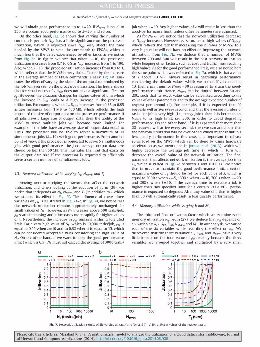
we will obtain good performance up to λ¼20. If NMWS is equal to350, we obtain good performance up to λ¼30, and so on.

On the other hand, Fig. 6c shows that varying the number ofcommands per task Ncpt has a little significance on the processorutilization, which is expected since Ncpt only affects the timeneeded by the MWS to send the commands to FPGAs, which ismuch less that the delay experienced by other tasks, as we noticefrom Fig. 6c. In figure, we see that when λ¼10, the processorutilization increases from 0.7 to 0.8 as Ncpt increases from 1 to 100.Also, when λ¼13, the processor utilization increases from 0.9 to 1,which reflects that the MWS is very little affected by the increasein the average number of FPGA commands. Finally, Fig. 6d illus-trates the effect of varying the size of the output data produced bythe job (on average) on the processor utilization. The figure showsthat for small values of λ, SOD does not have a significant effect onρp. However, the situation changes for higher values of λ, in whichthe increase in SOD leads to a high increase in the processorutilization. For example, when λ¼5, ρp increases from 0.35 to 0.85as SOD increases from 1 MB to 100 MB, which reflects the highimpact of the size of output data on the processor performance. Ifall jobs have a large size of output data, then the ability of theMWS to serve multiple jobs will become more limited. Forexample, if the jobs have an average size of output data equal to5 MB, the processor will be able to server a maximum of 10simultaneous jobs (λ¼10) with good performance. From anotherpoint of view, if the processor is requested to serve 5 simultaneousjobs with good performance, the job's average output data sizeshould be less than 50 MB. This illustrates the limit that exists onthe output data size if the processor is requested to efficientlyserve a certain number of simultaneous jobs.

4.3. Network utilization while varying Nt, NMWS, and Tj

Moving next to studying the factors that affect the networkutilization, and when looking at the equation of ρN in (29), wenotice that it depends on Nt , NMWS, and Tj (in addition to λ whichwe studied its effect in Fig. 5). The influence of these threevariables on ρN is illustrated in Fig. 7a–c. In Fig. 7a, we notice thatthe network utilization remains approximately unchanged forsmall values of Nt . However, as Nt increases above 500 tasks/job,ρN starts increasing and it increases more rapidly for higher valuesof λ. Nevertheless, the increase in ρN remains within a toleratedlimit. For a very high value of Nt , which is 10,000 tasks/job, ρN isequal to 0.55 when λ¼10 and to 0.82 when λ is equal to 15, whichcan be considered acceptable vales considering the high value ofNt . On the other hand, if we want to keep the good-performancelimit (which is 0.5), Nt must not exceed the average of 3000 tasks/

job when λ¼10. Any higher values of λ will result in less than thegood-performance limit, unless other parameters are adjusted.

As for NMWS, we notice that the network utilization decreasesas NMWS increases. However, ρN saturates at high values of NMWS,which reflects the fact that increasing the number of MWSs to avery high value will not have an effect on improving the networkutilization. From Fig. 7b, we deduce that a number of MWSsbetween 200 and 300 will result in the best network utilization,while keeping other factors, such as cost and traffic, from reachinghigh values. As for the good performance limit, we also notice herethe same point which was reflected in Fig. 7a, which is that a valueof λ above 10 will always result in degrading performance,considering the default values which we stated. If λ is equal to10, then a minimum of NMWS¼30 is required to attain the good-performance limit. Hence, NMWS can be limited between 30 and200, such that its exact value can be calculated according to thevalues of other parameters, and to the average expected number ofrequest per second (λ). For example, if it is expected that 10requests will arrive every second, and that the average number oftasks per job is very high (i.e., heavy jobs), then it is better to setNMWS to its high limit, i.e., 200, in order to avoid degradingperformance. On the other hand, if it is expected that more than20 requests will arrive every second, then we can anticipate thatthe network utilization will be overloaded which might result in aless-quality performance. In this case, it is important to releasesome load on the MWS, which can be done by using hardwareacceleration as we mentioned in Jomaa et al. (2013), which willhighly decrease the average job time Tj, which in turn willdecrease the overall value of the network utilization. The finalparameter that affects network utilization is the average job timeTj, which is varied in Fig. 7c between 1 and 10,000 s. We noticethat in order to maintain the good-performance limit, a certainmaximum value of Tj should be set for each value of λ, which isequal to 3000 s when λ¼5, 1800 s when λ¼10, 700 s when λ¼20,and 290 s when λ¼30. If the average time to execute a job ishigher than this specified limit for a certain value of λ, perfor-mance is expected to degrade. Also, any value of λ that is higherthan 30 will automatically result in less quality performance.

4.4. Memory utilization while varying k and MT

The third and final utilization factor which we examine is thememory utilization ρM . From (27), we deduce that ρM depends onsix variables: k, λ, SID, SOD, NMWS, and MT . In our analysis, we variedeach of the six variables while recording the effect on ρM . Wediscovered that the three variables SID, SOD, and NMWS have a verylittle impact on the total value of ρM , mainly because the threevariables are grouped together and multiplied by a very small

00.10.20.30.40.50.60.70.80.91

1.11.2

1 10 100 1000 10000

Util

izat

ion

Nt (tasks/job)

λ = 1 λ = 5 λ = 10λ = 15 λ = 20

00.10.20.30.40.50.60.70.80.91

1.11.2

10 100 1000

Util

izat

ion

NMWS

λ = 1 λ = 5 λ = 10λ = 15 λ = 20

00.10.20.30.40.50.60.70.80.91

1.11.2

1 10 100 1000 10000

Util

izat

ion

Tj (sec)

λ = 1 λ = 5 λ = 10λ = 20 λ = 30 λ = 50

Fig. 7. Network utilization results while varying Nt (a), NMWS (b), and Tj (c) for different values of the request rate λ.






constant (63�10�3), as compared to the other three variables(k, λ, andMT ). Hence, we do not show here the insignificant resultsof varying SID, SOD, and NMWS. Rather, we focus on the results of kand MT , which have an influence on the total value of ρM (havingalready presented the results of λ in Fig. 5). These results areshown in Fig. 8a, which shows the effect of varying the averagenumber of FPGAs per MWS on which a job is executed (k) on thememory utilization for different values of λ, and in Fig. 8b, whichdepicts the effect of varying k on ρM , but for different values of thetotal memory MT . First, from Fig. 8a, we deduce that as k increases,the memory utilization linearly increases. This increase is constantfor any value of λ, i.e., the value of ρM is approximately indepen-dent of the value of λ, a fact which we also observed in Fig. 5. Also,the maximum value of ρM , which is obtained when k is equal to 15FPGAs per job, is 0.6, which is much less than the good-performance limit, which is 0.85. Hence, the MWS memory in allcases that we studied will remain under-utilized and will not be aperformance bottleneck for the MWS. Finally in Fig. 8b, weobserve the effect of varying the total memory of the MWS MT

on ρM . We can see that when MT is less than 6 GB, thememory utilization will be high if the job is executed onmany FPGAs, mainly because of the large amounts of job dataand tasks that need to be saved. However, any value of MT

higher than 6 GB insures a good memory performance for allvalues of k.

4.5. Comparing with prototype results

A very important part of our analysis is to verify the model'sresults by comparing them to those obtained from testing a realcluster. To achieve this, we built a sample cloud prototype thatconsisted of five MWS servers that where connected via a high-speed router to form a sample cloud cluster. Each MWS is an Intel i7processor with 6 GB RAM running at 3.4 GHz, and connected via aswitch to two Xilinx Virtex 6 FPGAs. The MapReduce jobs that wererun by the MWSs on the FPGAs represented three applicationswhich we have used in Jomaa et al. (2013) and Mershad et al. (2013),and are part of The Phoenix benchmark (Yoo et al., 2009) that offersa variety of workloads and emphasis on communication andcomputation. These applications are String Matching (SM),K-means (KM), and Matrix Multiplication (MM). For the stringmatching application, a master document representing a researchpublication was searched for a keyword to return a list of sentencesthat contain it, if any. The string whose length ranged between 5 and22 characters was randomly selected from a list of 48 keywords,whereas the selected document was one of 25 conference and

journal papers ranging in length from 5112 to 11,674 words. As forthe k-means application, we used a dataset containing 20 millionpoints in a 2D space, whereas the number of centroids wasrandomly set to a value between 2 and 32. Finally, the matrixmultiplication application, calculates the product of two inputmatrices containing integer values and randomly picked from a setof two pairs, with dimensions of (100�150, 150�100) and(400�400, 400�400), respectively.

The string matching application is a series of MapReduce Jobs,where each job is assigned a keyword and a buffer that is used tohold a single line from the document to be searched. Theencapsulated Map tasks look for keyword matches in the assignedbuffers, and the results are sent to a Reduce task for overallordering of matches in the document. For K-Means clustering, the2D points are grouped into vectors that are assigned to Map tasks.Each task is responsible for computing the Euclidian distancesbetween the various data points in its assigned data vector and theK centroids. The distances are sent to a Reduce task to recalculatethe nearest centroids. Finally, in matrix multiplication, each Maptask multiplies a row in the left matrix and a column in the rightmatrix, whereas the Reduce task performs the addition.

The input data to the applications were distributed uniformlyamong the ten FPGAs. To each MWS, a laptop is connected via adedicated Ethernet cable, and representing a client that sendsMapReduce jobs to the MWS. During the testing time, each clientchoses randomly one of the three applications, formulates aMapReduce job with random but realistic input parameter values,and sends the job to the MWS to which it is connected. The MWS,after receiving the job from the client, distributes it to one or moreFPGAs, including those attached to other MWSs. This operation isrepeated by each client according to the desired value of λ in thetesting scenario.

In order to make a fair comparison between the mathematicaland the prototype results, we saved all parameters that were usedwhen running the testing scenarios, and used them in the analysisequations. For each MapReduce job that is executed during atesting scenario, we save to a log file the job parameters, inputs,and outputs; and at the end of the testing scenario, we calculatethe average values for all jobs that were executed in the scenario.For example, we found that the average job input and output sizesin the testing scenarios were about 9.67 MB and 122 KB, respec-tively, and hence, we set the value of SID and SOD in themathematical model's equations to 10,139,730 and 124,928 bytes,respectively. Similarly, based on the average values calculated fromthe testing scenarios, we found that the average number of tasksper job was equal to 20, the average number of commands per task

0

0.1

0.2

0.3

0.4

0.5

0.6

0.7

0 1 2 3 4 5 6 7 8 9 10 11 12 13 14 15

Util

izat

ion

k (FPGAs/job)

λ = 1 λ = 5 λ = 10λ = 20 λ = 30

00.10.20.30.40.50.60.70.80.91

1.11.2

0 1 2 3 4 5 6 7 8 9 10 11 12 13 14 15

Util

izat

ion

k (FPGAs/job)

MT = 0.5 GB MT = 2 GB MT = 6 GBMT = 10 GB MT = 20 GB

Fig. 8. Memory utilization results while varying the number of FPGAs per job (k) for different values of the request rate λ (a), and for different values of the total memoryMT (b).







https://www.researchgate.net/publication/221474571_Phoenix_rebirth_Scalable_MapReduce_on_a_large-scale_shared-memory_system?el=1_x_8&enrichId=rgreq-0006c4b32020d6e30a3c49a7f94426d1-XXX&enrichSource=Y292ZXJQYWdlOzI2NTE2OTkxMjtBUzoxODk0MTYxOTA1MjEzNTFAMTQyMjE3MTc0NzYzNw==

was equal to 10, and the average time for a job to finish executionwas equal to 1391 seconds. Hence, we set Nt to 20, Ncpt to 10, andTj to 1391. Finally, it is important to note that the five MWSsshared a network link of 1 Mbps, and therefore, we consideredthat the bandwidth of each MWS will be 200 Kbps when calculat-ing the value of B0.

The prototype results were calculated using the PerformanceMonitor tool that is part of Microsoft Windows. We usedcustom counters that we designed to only track related applicationnetwork traffic, plus CPU and memory utilizations. On each MWS,we run the Performance Monitor tool during the testing scenarioto save to a custom data collector set the amount of CPU andMemory utilizations, and network bandwidth that are consumedby each running process. The data collector collects and saves thisdata based on constant time intervals. After the testing scenariofinishes, we identify from the output of the data collector set, theprocesses that are related to our system. Then we calculate thetotal CPU, Memory, and Network bandwidth consumed by theseprocesses, and the average utilization of the CPU, Memory, andNetwork link during the testing scenario. We performed ninetesting scenarios, in which λ was varied between 1 and 40, withintervals of 5 (i.e., 1, 5, 10, 15 …). The calculated results, alongsidethe analysis equations results for the corresponding parameters ofthis section, are shown in Fig. 9a, b, and c.

In Fig. 9a, we notice the same trend of the prototype and themathematical results of the CPU utilization, but the prototype resultsare more affected by λ. The error margin between the two results isabout 0.15 between λ¼1 and λ¼25. After λ¼30, both resultsconverge to 1 and the processor will be working at full utilization.The good performance limit is achieved by the prototype at λ¼18,while with the mathematical model it is reached at λ¼23. The smallerror margin between the prototype and the mathematical analysisresults of Fig. 9a proves that our mathematical model depicts, to ahigh level of accuracy, the CPU utilization of the MWS. On the other,with respect to the network utilization in Fig. 9b, the error margin isabout 0.03 between λ¼1 and λ¼10, but increases to 0.07 for valuesof λ between 25 and 35. After λ¼35, both results converge to 1, andthe network link will be working at full utilization. The network goodperformance limit is achieved by the prototype at λ¼18 and by themodel at λ¼22. The error margin between the prototype and themathematical model is smaller for the network utilization resultsthan the CPU utilization results. However, both can be considered asaccepted error margins. Most importantly, both prototype and modelresults converge at near values (30 for the CPU utilization and 40 forthe network utilization). Finally, Fig. 9c shows the memory utilizationresults, where we notice that the model's memory utilizationincreases at a low rate, as λ increases between 1 and 40. On the

other hand, the prototype's memory utilization increases at a slightlyhigher rate. However, this rate decreases as λ increases. After λ¼30,we notice that the prototype results starts converging. The errormargin is the lowest here, with an average value of 0.023.

Overall, the small error margins between the prototype and themathematical model results, and the fact that they converge atsimilar values of λ proves the accuracy of our model in depictingthe CPU, Memory, and Network utilizations.

5. Concluding remarks

In this paper, we presented a novel mathematical model thatanalyzes the performance of the Middleware Server (MWS) of adistributed framework for data-intensive applications that wepresented in Abbani et al. (2011) under the name of the RASSDplatform. The mathematical model focused on deriving equationsthat illustrate the load on the MWS from three perspectives:processor, memory, and network interface. The aim was tocalculate the utilization of each of the three domains in terms ofthe parameters that affect it. We studied the various operationsand processes that have an influence of each of the three domains,and so we divided these operations into separate parts andcalculated the equation for each part in terms of its own para-meters. In order to reach our objective, we investigated the bestapproach for each of the three utilizations: for processor utiliza-tion, we studied the various operations that consume a certaintime inside the MWS CPU, and derived an equation of the delay ofeach operation. For memory utilization, we defined the tasks thatare executed by the MWS and that require saving data inside theprocessor memory and we derived an equation for the amount ofmemory needed by each task. For network utilization, we pointedout the various communications that might occur between theMWS and external entities and derived an equation for the totalamount of bytes exchanged in each communication. Using thesecalculated equations, we were able to determine each of the threeutilizations in terms of the variables that might take differentvalues depending on the system status and circumstances, afterwe find out the average values of other parameters that can beassigned an average constant based on previous literature worksand based on our own simulations. The obtained results provedthat memory utilization is in most cases within its good-performance limit, meaning that it does not constitute a perfor-mance bottleneck for the MWS, unless in very severe load cases.As for the processor utilization, we found that it is mostly affectedby the overall jobs' characteristics, such as the average number oftasks in the job (which can be directly related to the amount of

00.10.20.30.40.50.60.70.80.91

1.1

0 5 10 15 20 25 30 35 40

CPU

Util

izat

ion

λ (requests/sec)

Analysis

Prototype0

0.10.20.30.40.50.60.70.80.91

1.1

0 5 10 15 20 25 30 35 40

Net

wor

k U

tiliz

atio

n

λ (requests/sec)

Analysis

Prototype

00.020.040.060.080.10.120.140.160.180.2

0 5 10 15 20 25 30 35 40

Mem

ory

Util

izat

ion

λ (requests/sec)

Analysis

Prototype

Fig. 9. Comparison of CPU (a), Network (b), and Memory (c) utilizations for the prototype and the mathematical analysis while varying λ.







execution in the job) and the average size of the jobs' output data.With respect to network utilization, we found that it is mostlyaffected by the average jobs' execution time. For both utilizations,we defined the limits for good-performance and the values ofvarious variables that will keep the MWS performance withinthese limits. We discussed the effects of changing one or multiplevariables simultaneously on the MWS performance, and themeasures that could be taken to avoid poor performance. Forfuture work, we aim at comparing the performance of our system,both analytically and via simulations, with other similar systems,such as the Hadoop framework.

Acknowledgment

This work was supported by NPRP grant # 09-155-2-066 fromthe Qatar National Research Fund (a member of Qatar Foundation).The statements made therein are solely the responsibility of theauthors.

References

Abbani N, Ali A, Al Otoom D, Jomaa M, Sharafeddine M, Artail H, Akkary H, Saghir M,Awad M, Hajj H. A distributed reconfigurable active SSD platform for dataintensive applications. In: Proceedings of IEEE 13th international conference onHigh Performance Computing and Communications (HPCC); September 2011.

Agus T, Suied C, Thorpe S, Pressnitzer D. Characteristics of human voice processing.In: Proceedings of IEEE International Symposium on Circuits and Systems(ISCAS 2010). Paris, France; June 2010.

Ali A, Jomaa M, Romanous B, Sharafeddine M, Saghir M, Akkary H, Artail H, Awad M,Hajj H. An operating system for a reconfigurable active SSD processing node. In:Proceedings of the 19th International Conference on Telecommunications (ICT2012). Jounieh, Lebanon; April 2012.

CISCO Financial Services Technical Decision Maker White Paper: Design BestPractices for Latency Optimization. Available online: ⟨www.cisco.com/application/pdf/en/us/guest/netsol/ns407/c654/ccmigration_09186a008091d542.pdf⟩.

Cao J, Andersson M, Nyberg C, Kihl M. Web server performance modeling using anm/g/1/kn ps queue. In: Proceedings of the 10th International Conference onTelecommunications ICT (2003). Tahiti, Papeete, French Polynesia; February2003.

Celimaris Vega Citrix Consulting. MetaFrame XP Oracle 11i Scalability Analysis.Available online: ⟨http://support.citrix.com/article/CTX101887⟩.

Cho J, Garcia-Molina H. Estimating frequency of change. ACM Trans InternetTechnol 2003;3(3):256–90.

Curran K, Duffy C. Understanding and reducing web delays. Int J Netw Manag2005;15(2):89–102.

Dean J. Software engineering advice from building large-scale distributed systems.Available online: ⟨http://research.google.com/people/jeff/stanford-295-talk.pdf⟩.

Ebbers M. Turning big data into actionable information with IBM InfoSpherestreams, IBM Redbooks Solution Guide. January 2013.

Herodotou H. Hadoop Performance Models, technical report CS-2011-05, dukecomputer science. Available online: ⟨http://www.cs.duke.edu/starfish/files/hadoop-models.pdf⟩; 2011.

How long does it take to make a context switch? Available online: ⟨http://blog.tsunanet.net/2010/11/how-long-does-it-take-to-make-context.html⟩.

Jomaa M , Mershad K, Abbani N, Sharaf-Dabbagh Y, Romanous B, Artail H, Saghir M,Hajj H, Akkary H, Awad M. A mediation layer for connecting data-intensiveapplications to reconfigurable data nodes. In: Proceedings of the InternationalConference on Computer Communications and Networks (ICCCN 2013). Nassau,Bahamas; July 2013.

Kelly L. Big data and analytics: a large challenge offering great opportunities,Computer Weekly. Available online: ⟨http://www.computerweekly.com/feature/Big-data-and-analytics-a-large-challenge-offering-great-opportunities⟩.

Larsen S, Sarangam P, Huggahalli R. Architectural breakdown of end-to-end latencyin a TCP/IP Network. Proceedings of the 19th international symposium oncomputer architecture and high performance computing (SBAC-PAD 2007).Gramado, RS, Brazil; October 2007.

Litwin W, Risch T. Main memory oriented optimization of OO queries using typeddatalog with foreign predicates. IEEE Trans Knowl Data Eng 1992;4(6):517–28.

Mershad K, Kaitoua A, Artail H, Saghir M, Hajj H. A framework for multi-cloudcooperationwith hardware reconfiguration support. In: Proceedings of IEEE 9thworld congress on services (SERVICES 2013). Santa Clara, CA; June 2013.

Ramon M, Caharel S, Rossion B. The speed of recognition of personally familiarfaces. Perception 2011;40(4):437–49.

Rodriguez-Martinez M, Roussopoulos N. MOCHA: a self-extensible database mid-dleware system for distributed data sources. In: Proceedings of the 2000 ACMSIGMOD international conference on Management of data (SIGMOD 000), vol.29. June 2000. p. 213–24.

Using – Xss to adjust Java default thread stack size to save memory and preventStackOverflowError. Available online: ⟨http://www.onkarjoshi.com/blog/209/using-xss-to-adjust-java-default-thread-stack-size-to-save-memory-and-prevent-stackoverflowerror/⟩.

Yoo R, Romano A, Kozyrakis C. Phoenix rebirth: Scalable MapReduce on a large-scale shared-memory system. IISWC’09. Austin, TX; October 2009.



http://www.cisco.com/application/pdf/en/us/guest/netsol/ns407/c654/ccmigration_09186a008091d542.pdf

http://www.cisco.com/application/pdf/en/us/guest/netsol/ns407/c654/ccmigration_09186a008091d542.pdf

http://support.citrix.com/article/CTX101887

http://refhub.elsevier.com/S1084-8045(14)00192-1/sbref1




http://research.google.com/people/jeff/stanford-295-talk.pdf

http://www.cs.duke.edu/starfish/files/hadoop-models.pdf

http://www.cs.duke.edu/starfish/files/hadoop-models.pdf

http://blog.tsunanet.net/2010/11/how-long-does-it-take-to-make-context.html

http://blog.tsunanet.net/2010/11/how-long-does-it-take-to-make-context.html

http://www.computerweekly.com/feature/Big-data-and-analytics-a-large-challenge-offering-great-opportunities

http://www.computerweekly.com/feature/Big-data-and-analytics-a-large-challenge-offering-great-opportunities





http://www.onkarjoshi.com/blog/209/using-xss-to-adjust-java-default-thread-stack-size-to-save-memory-and-prevent-stackoverflowerror/





















https://www.researchgate.net/publication/232653720_Main_Memory_Orientated_Optimization_of_OO_Queries_Using_Typed_Datalog_with_Foreign_Predicates?el=1_x_8&enrichId=rgreq-0006c4b32020d6e30a3c49a7f94426d1-XXX&enrichSource=Y292ZXJQYWdlOzI2NTE2OTkxMjtBUzoxODk0MTYxOTA1MjEzNTFAMTQyMjE3MTc0NzYzNw==

https://www.researchgate.net/publication/232653720_Main_Memory_Orientated_Optimization_of_OO_Queries_Using_Typed_Datalog_with_Foreign_Predicates?el=1_x_8&enrichId=rgreq-0006c4b32020d6e30a3c49a7f94426d1-XXX&enrichSource=Y292ZXJQYWdlOzI2NTE2OTkxMjtBUzoxODk0MTYxOTA1MjEzNTFAMTQyMjE3MTc0NzYzNw==



















a mathematical model to analyze the utilization of a cloud datacenter middleware

Documents