data mining approach to analyze mobile telecommunication
TRANSCRIPT
ADDIS ABABA UNIVERSITY
SCHOOL OF GRADUATE STUDIES
SCHOOL OF INFORMATION SCIENCE
DATA MINING APPROACH TO ANALYZE
MOBILE TELECOMMUNICATIONS NETWORK
QUALITY OF SERVICE: THE CASE OF ETHIO-
TELECOM
LULU DEYU
MAY 2014
SCHOOL OF GRADUATE STUDIES
SCHOOL OF INFORMATION SCIENCE
DATA MINING APPROACH TO ANALYZE
MOBILE TELECOMMUNICATIONS NETWORK
QUALITY OF SERVICE: THE CASE OF ETHIO-
TELECOM
A Thesis Submitted to the School of Graduate Studies of
Addis Ababa University in Partial Fulfillment of the
Requirements for the Degree of
Masters of Science in Information Science
BY
LULU DEYU
MAY 2014
ADDIS ABABA UNIVERSITY
SCHOOL OF GRADUATE STUDIES
SCHOOL OF INFORMATION SCIENCE
DATA MINING APPROACH TO ANALYZE MOBILE
TELECOMMUNICATIONS NETWORK QUALITY OF SERVICE:
THE CASE OF ETHIO-TELECOM
BY
LULU DEYU
Name and Signature of Members of the Examining Board
Name Title Signature Date
Ato Getachew Jemaneh Advisor ___________ __________
Dr. Martha Yifru Examiner ___________ __________
Ato Michael Melese Chair person __________ _________

i
Acknowledgement
I gratefully acknowledge the support and guidance of my advisor Ato Getachew Jemaneh. I
would not imagine completing this work without all his scholarly advices. I am deeply indebted
to him for his critical readings and constructive comments. I would like also to express my
gratitude to all my instructors whose contribution helped me to succeed on this study.
I would like to express my deep gratitude and appreciation to the ethio telecom Engineering as
well as Operation and Maintenance departments, especially, Ato Ashagre Getenet and his mobile
optimization team, Ato Gebru Kerse and his team for their dedicated support in my study.
Last but not least, my deepest thank goes to my family for their emotional support and
encouragement.
ii
Acronyms
2G Second Generation
3G Third Generations
3GPP Third Generation Partnership Project
AGCH Access grant channel
ARFF Attribute Relation File Format
ANSI American National Standards Institute
ARIB Alliance of Radio Industries and Business
AUC Authentication Centre
BCCH Broadcast control channel
BSS Base Station Subsystem
BTS Base Transreceiver Station
CART Classification and Regression Trees
CCCH Common control channel
CCH Control channels
CDMA Code Division Multiple Access
CDR Call Drop Rate
CRISP CRoss-Industry Standard Process
CSR Call Success Rate
CSSR Call Set-Up Success Rate
DAMA Demand -Assigned Multiple Access
CSV Comma Separated Value
DCCH Dedicated control channel
DNS Domain Name Servers
EDGE Enhanced Data rates in GSM Environment
EFY Ethiopian Fiscal Year
EIR Equipment Identity Registers
ETSI European Telecommunication Standard Institute
FACCH Fast associated dedicated control channel
FCCH Frequency correction channel
iii
FDMA Frequency Division Multiple Access
FP-growth Frequent Pattern growth
GGSN Gateway GPRS Support Node
GPRS General Packet Radio Service
GSM Global Standard for Mobile Communication
HLR Home Location Register
HOSR Handover Success Rate
ICT Information Communication Technology
IP Internet Protocol
ISDN Integrated Switch Digital Network
ITU International Telecommunication Union
KDD Knowledge Data Discovery
KPI Key Performance Indicator
KQI Key Quality Indicator
LAC Location area code
LAPD Link Access Protocol for D-channel
LTE Long Term Evolution
MLP Multi-Layer Perception
MSC Mobile Switching Control
NMS Network Management System
NP Network Performance
NSS Network Switching Subsystem
O&M Operation and Maintenance
PCH Paging Channel
PSTN Public Switch Telephone Network
QoS Quality of Service
RACH Random access channel
RAN Radio Access Network
RF Radio Frequency
SACCH Slow associated dedicated control channel
SCH Synchronization channel
iv
SDCCH Stand-alone dedicated control channel
SGSN Serving GPRS Support Node
SMS Short Message Service
SMSC Short Message Service Centre
SOM Self-Organizing Map
SS Spread Spectrum
SS7 Signaling system no. 7
TCH Traffic channels
TCHCR TCH Congestion Rate
TCSM Transcoder sub-multiplexer
TMN Telecom Management Network
TRX Transceivers
TS Time slots
UMTS Universal Terrestrial Mobile System
VAS Value Added Services
VAS IN VAS INtelligent services
VLR Visitor Location Register
VMS Voice Mail System
WCDMA Wide band Code Division Multiple Access

v
Table of Contents
Acknowledgement .......................................................................................................................... i
Acronyms ....................................................................................................................................... ii
List of Tables ................................................................................................................................. x
List of Figures .............................................................................................................................. xii
Abstract ....................................................................................................................................... xiii
Chapter One .................................................................................................................................. 1
1. Introduction ............................................................................................................................. 1
1.1 Background ...................................................................................................................... 1
1.2 Statement of the problem ................................................................................................. 4
1.3 Objectives of the Study .................................................................................................... 6
1.3.1 General Objective ..................................................................................................... 6
1.3.2 Specific Objectives ................................................................................................... 6
1.4 Scope and Limitation ....................................................................................................... 6
1.5 Significance of the Study ................................................................................................. 7
1.6 Research Methodology ..................................................................................................... 7
1.7 Expected Findings and Summary ..................................................................................... 8
1.8 Organization of the Research ........................................................................................... 8
Chapter Two .................................................................................................................................. 9
2 Mobile Cellular Network and Quality of Service .................................................................... 9
2.1 Overview of Mobile Communication in Ethiopia and the World .................................... 9
2.2 Standardization Bodies in Mobile Technology .............................................................. 10
2.3 Evolution of Mobile Network ........................................................................................ 10
2.3.1 The First-generation System (Analogue) ................................................................ 11
2.3.2 The Second-generation System (Digital) ................................................................ 11
vi
2.3.3 Third-generation Networks (WCDMA in UMTS) ................................................. 12
2.3.4 Fourth-generation Networks (All-IP) ..................................................................... 12
2.4 Multiple-access Techniques ........................................................................................... 13
2.5 System Capacity ............................................................................................................. 13
2.5.1 Traffic Estimates ..................................................................................................... 14
2.5.2 Average Antenna Height......................................................................................... 14
2.5.3 Frequency Usage and Re-use .................................................................................. 15
2.6 Constituents of Mobile Networks .................................................................................. 15
2.6.1 Second Generation Network ................................................................................... 15
2.6.2 Third Generation Network ...................................................................................... 17
2.6.3 Fourth Generation (All IP) Network ....................................................................... 18
2.7 Telecommunications Management Network (TMN) ..................................................... 19
2.8 Quality of Service (QoS) and Network Performance (NP) ............................................ 21
2.9 Radio Access Network Key Performance Indicators (RAN KPIs) ................................ 23
2.9.1 Logical Channels .................................................................................................... 24
2.9.2 Performance Measurement ..................................................................................... 25
Chapter Three ............................................................................................................................. 29
3 Data Mining and Knowledge Discovery ............................................................................... 29
3.1 Basic Concepts ............................................................................................................... 29
3.2 Data Mining Tasks ......................................................................................................... 30
3.2.1 Predictive Methods ................................................................................................. 30
3.2.2 Descriptive Methods ............................................................................................... 33
3.3 Challenges of Data Mining ............................................................................................ 35
3.4 Data Mining Process Models ......................................................................................... 37
3.4.1 KDD Process ........................................................................................................... 39
vii
3.4.2 CRISP-DM Process Model ..................................................................................... 40
3.5 Application of Data Mining in Telecommunications ..................................................... 42
3.5.1 Types of Telecommunication Data ......................................................................... 43
3.5.2 Data Mining Tasks in Telecommunications ........................................................... 44
3.5.3 Local Researches in the Telecom Industry ............................................................. 46
3.6 Review of Related works ............................................................................................... 47
Chapter Four ............................................................................................................................... 49
4 Data Mining Methods for QoS Management ........................................................................ 49
4.1 Decision Tree Classification .......................................................................................... 49
4.1.1 J48 Decision Tree Algorithm .................................................................................. 52
4.2 Naïve Bayes Classification............................................................................................. 54
4.2.1 Bays Theorem ......................................................................................................... 54
4.3 Neural Network .............................................................................................................. 56
4.3.1 Multilayer perception .............................................................................................. 57
4.4 k-Means Clustering ........................................................................................................ 59
4.4.1 k-Means Algorithm ................................................................................................. 60
Chapter Five ................................................................................................................................ 62
5 Experimentation and Analysis ............................................................................................... 62
5.1 Experiment Design ......................................................................................................... 62
5.2 KDD Processes ............................................................................................................... 62
5.2.1 Learning the application domain ............................................................................ 62
5.2.2 Creating target data set............................................................................................ 63
5.2.3 Data cleaning and preprocessing ............................................................................ 63
5.2.4 Data reduction ......................................................................................................... 66
5.2.5 Choosing the function of data mining ..................................................................... 77
viii
5.2.6 Choosing the data mining algorithm ....................................................................... 78
5.2.7 Data Mining ............................................................................................................ 78
5.3 Cluster Model ................................................................................................................. 79
5.3.1 Experiment 1 ........................................................................................................... 80
5.3.2 Experiment 2 ........................................................................................................... 82
5.3.3 Evaluation of the Discovered Knowledge .............................................................. 83
5.4 Classification Model ...................................................................................................... 85
5.4.1 J48 Decision Tree Classifier ................................................................................... 86
5.4.2 The Naïve Bayes Classifier ..................................................................................... 88
5.4.3 Multilayer Perception Classifier ............................................................................. 89
5.4.4 Comparison of J48, Naïve Bayes, and Multilayer Perception Models ................... 92
5.4.5 Evaluation of the discovered knowledge ................................................................ 94
Chapter Six .................................................................................................................................. 96
6 Conclusion and Recommendation ......................................................................................... 96
6.1 Conclusion ...................................................................................................................... 96
6.2 Recommendation ............................................................................................................ 98
References ..................................................................................................................................... 99
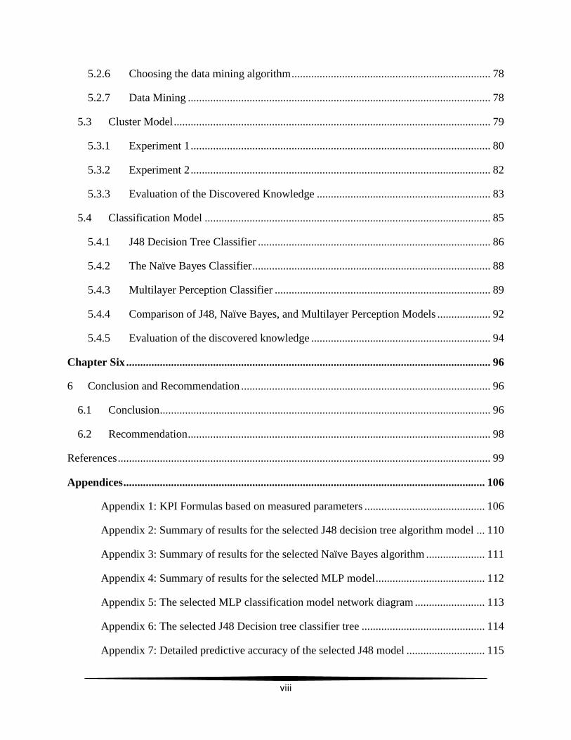
Appendices ................................................................................................................................. 106
Appendix 1: KPI Formulas based on measured parameters ........................................... 106
Appendix 2: Summary of results for the selected J48 decision tree algorithm model ... 110
Appendix 3: Summary of results for the selected Naïve Bayes algorithm ..................... 111
Appendix 4: Summary of results for the selected MLP model ....................................... 112
Appendix 5: The selected MLP classification model network diagram ......................... 113
Appendix 6: The selected J48 Decision tree classifier tree ............................................ 114
Appendix 7: Detailed predictive accuracy of the selected J48 model ............................ 115

ix
Appendix 8: Detailed predictive accuracy of the selected Naïve Bayes model ............. 116
Appendix 9: Detailed predictive accuracy of the selected MLP model .......................... 117
x
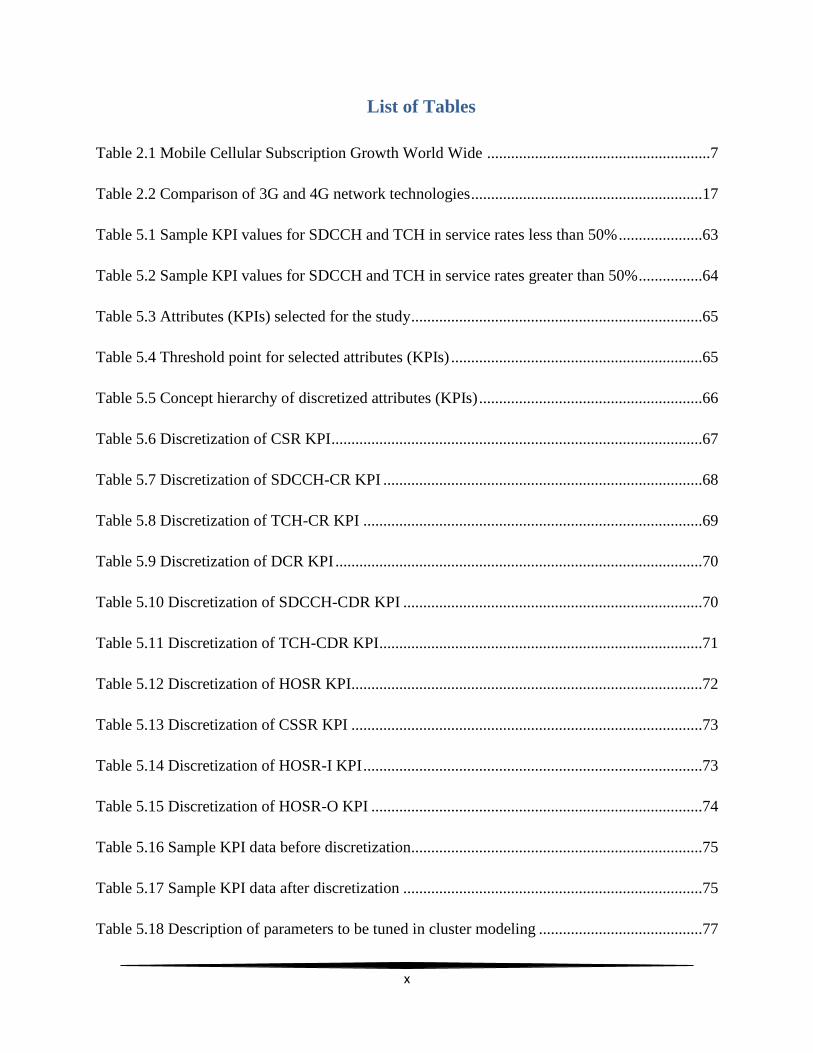
List of Tables
Table 2.1 Mobile Cellular Subscription Growth World Wide ........................................................7
Table 2.2 Comparison of 3G and 4G network technologies ..........................................................17
Table 5.1 Sample KPI values for SDCCH and TCH in service rates less than 50% .....................63
Table 5.2 Sample KPI values for SDCCH and TCH in service rates greater than 50% ................64
Table 5.3 Attributes (KPIs) selected for the study .........................................................................65
Table 5.4 Threshold point for selected attributes (KPIs) ...............................................................65
Table 5.5 Concept hierarchy of discretized attributes (KPIs) ........................................................66
Table 5.6 Discretization of CSR KPI .............................................................................................67
Table 5.7 Discretization of SDCCH-CR KPI ................................................................................68
Table 5.8 Discretization of TCH-CR KPI .....................................................................................69
Table 5.9 Discretization of DCR KPI ............................................................................................70
Table 5.10 Discretization of SDCCH-CDR KPI ...........................................................................70
Table 5.11 Discretization of TCH-CDR KPI .................................................................................71
Table 5.12 Discretization of HOSR KPI........................................................................................72
Table 5.13 Discretization of CSSR KPI ........................................................................................73
Table 5.14 Discretization of HOSR-I KPI .....................................................................................73
Table 5.15 Discretization of HOSR-O KPI ...................................................................................74
Table 5.16 Sample KPI data before discretization.........................................................................75
Table 5.17 Sample KPI data after discretization ...........................................................................75
Table 5.18 Description of parameters to be tuned in cluster modeling .........................................77
xi
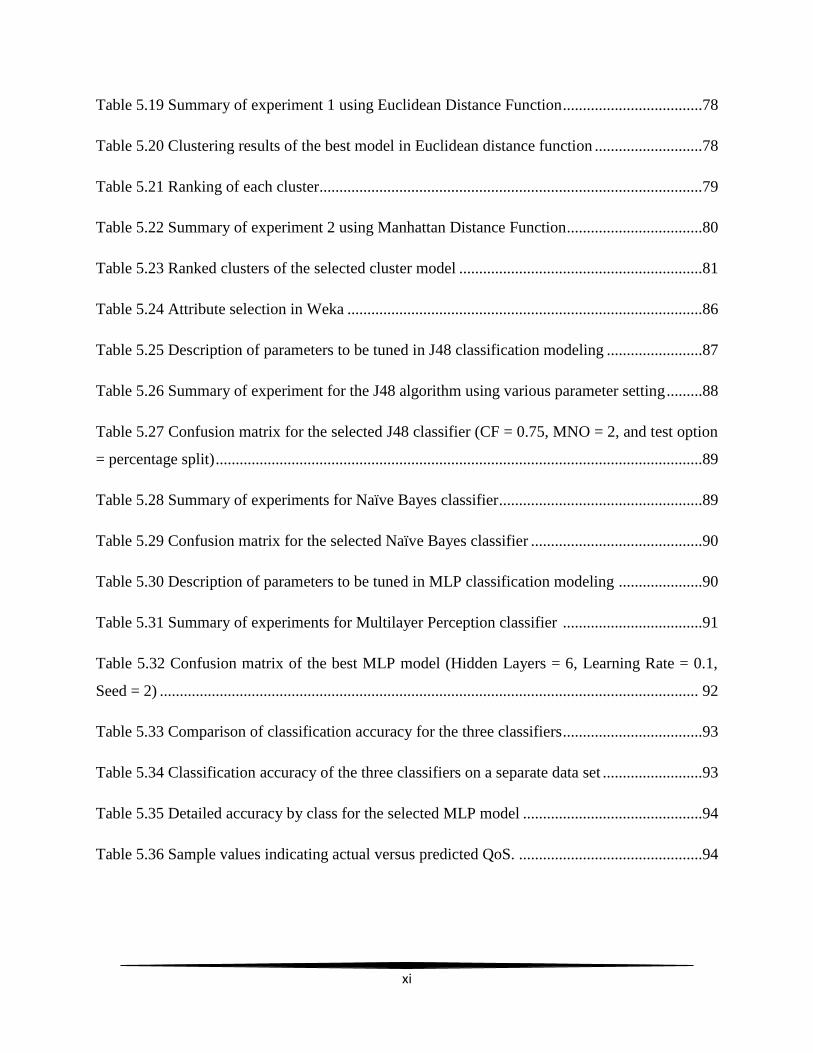
Table 5.19 Summary of experiment 1 using Euclidean Distance Function ...................................78
Table 5.20 Clustering results of the best model in Euclidean distance function ...........................78
Table 5.21 Ranking of each cluster................................................................................................79
Table 5.22 Summary of experiment 2 using Manhattan Distance Function ..................................80
Table 5.23 Ranked clusters of the selected cluster model .............................................................81
Table 5.24 Attribute selection in Weka .........................................................................................86
Table 5.25 Description of parameters to be tuned in J48 classification modeling ........................87
Table 5.26 Summary of experiment for the J48 algorithm using various parameter setting .........88
Table 5.27 Confusion matrix for the selected J48 classifier (CF = 0.75, MNO = 2, and test option
= percentage split) ..........................................................................................................................89
Table 5.28 Summary of experiments for Naïve Bayes classifier ...................................................89
Table 5.29 Confusion matrix for the selected Naïve Bayes classifier ...........................................90
Table 5.30 Description of parameters to be tuned in MLP classification modeling .....................90
Table 5.31 Summary of experiments for Multilayer Perception classifier ...................................91
Table 5.32 Confusion matrix of the best MLP model (Hidden Layers = 6, Learning Rate = 0.1,
Seed = 2) ....................................................................................................................................... 92
Table 5.33 Comparison of classification accuracy for the three classifiers ...................................93
Table 5.34 Classification accuracy of the three classifiers on a separate data set .........................93
Table 5.35 Detailed accuracy by class for the selected MLP model .............................................94
Table 5.36 Sample values indicating actual versus predicted QoS. ..............................................94
xii
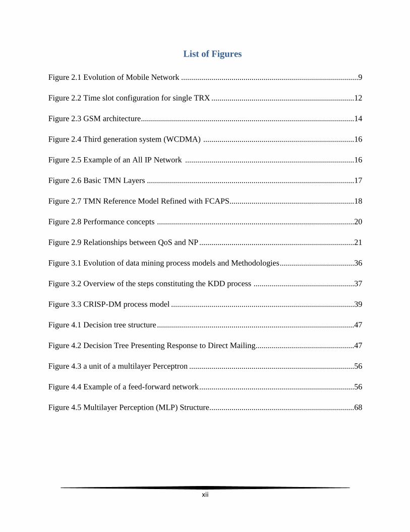
List of Figures
Figure 2.1 Evolution of Mobile Network ........................................................................................9
Figure 2.2 Time slot configuration for single TRX .......................................................................12
Figure 2.3 GSM architecture..........................................................................................................14
Figure 2.4 Third generation system (WCDMA) ...........................................................................16
Figure 2.5 Example of an All IP Network ....................................................................................16
Figure 2.6 Basic TMN Layers .......................................................................................................17
Figure 2.7 TMN Reference Model Refined with FCAPS..............................................................18
Figure 2.8 Performance concepts ..................................................................................................20
Figure 2.9 Relationships between QoS and NP .............................................................................21
Figure 3.1 Evolution of data mining process models and Methodologies .....................................36
Figure 3.2 Overview of the steps constituting the KDD process ..................................................37
Figure 3.3 CRISP-DM process model ...........................................................................................39
Figure 4.1 Decision tree structure ..................................................................................................47
Figure 4.2 Decision Tree Presenting Response to Direct Mailing.................................................47
Figure 4.3 a unit of a multilayer Perceptron ..................................................................................56
Figure 4.4 Example of a feed-forward network .............................................................................56
Figure 4.5 Multilayer Perception (MLP) Structure........................................................................68
xiii
Abstract
Huge amount of measurement data indicating the performance of a mobile network has been
generated. Sometimes it is very difficult to draw essential information from this complex data
merely applying domain expertise and prior knowledge. For the ultimate goal of QoS
improvement, it is helpful to follow a data mining approach to deal with this complex data.
In this study, a sample data on three time stamps such as 24-hour, 1-month, and 1-week day and
night high traffic hours, indicating QoS KPIs has been taken from the live network of ethio
telecom. Strictly following the KDD process, various experiments are conducted using the Weka
open source data mining tool. This is done to find out the number of clusters that logically
segment the KPI data applying the simple k-means algorithm and the best classification model
comparing the J48 decision tree, the Naïve Bayes, as well as the Multilayer Perception
classifiers.
It has been found that the cluster model worth splits the KPI data in to five clusters on the basis
of their natural proximity. These clusters are ranked and labeled to be applied on the next
classification model experiment. In this experiment a data set of four selected attributes and 8478
instances has been used to build and select the best model. A separate data set of 4240 instances
is provided to finally evaluate the classification accuracy of the selected model for unseen data.
As a result a classification model built on Multilayer Perception with 6 ‗Hidden Layers‘,
‗Learning Rate‘ of 0.1 and ‗ Seed‘ value of 2 has got the best classification accuracy by correctly
classifying 84.4953 % of the data in to their classes.
Key Words: QoS, KPI, KDD process.
Data Mining Approach to Analyze Mobile Telecommunication Network QoS: The case of ethio telecom
1
Chapter One
1. Introduction
1.1 Background
The application of data mining for any industry generally depends on the availability of data and
business challenges that reside in the industry as described in Weiss (2009). In this regard, the
telecommunications industry generates high quality data from its network operation and the
occurrence of large customer that rely on the network infrastructure. Those data generated as a
result of the business operation of telecommunications include phone call data regarding each
call conducted by the customer in the form of call detail record, billing information that details
about the payment to be discharged together with the customer profile, and data generated as a
result of the network operations. On the other hand this telecom industry faces enormous
business challenges such as how to improve the functionality of its market, how to detect and
prevent fraudulent call activities, as well as how to plan and optimize the network and manage
the recurring fault. Acting up on the routinely generated huge data, these business challenges can
be resolved through the application of data mining.
There are also so many data mining challenges in applying the telecommunications data for data
mining. As discussed in Weiss (2009) these challenges include the scale of the data in the large
telecommunications database, the raw data needs to be summarized based on important features
to make it suitable for data mining, predicting very rare events such as detecting a fraudulent call
activity from the time series data that represent individual events, as well as many data mining
models such as fraud detection and network fault isolation needs to be applied in real time.
Data mining technology solve problems through the analysis of data already exist in databases.
As the observed data sets are grown in size and complexity there is a need to automatically
analyze these data using data mining technology through the application of different intelligent
algorithms such as neural networks, decision trees, association rules and others, Pitas et al
(2011). When it comes to mobile network quality of service (QoS), the observational data for
Data Mining Approach to Analyze Mobile Telecommunication Network QoS: The case of ethio telecom
2
performance measurement could be captured from the live network through drive test
measurement or from the network management system database.
It is the user expectations that constitute the Quality of Service (QoS), which is defined as "the
collective effect of service performances, which determine the degree of satisfaction of a user of
the service‖ ITU-T E.800 (1988), pp. 3. This general definition means that a single QoS measure
is not possible. In this regard, Hardy (2001) has specified three notions of QoS, which are
intrinsic, perceived, and assessed quality of service. Intrinsic quality is achieved via the
technical design of the transport network and terminations, which determine the characteristics
of the connections made through the network, and provisioning of network accesses,
terminations, and switch-to-switch links, which determines whether the network will have
adequate capacity to handle the anticipated demand. Perceived QoS resulted from user
experiences when a service is being used. Assessed QoS indicates the value of continued use of
a service for the user who pays for it.
Suutarinen (1994) develop a solution for quality performance measurement to manage the
performance of a GSM base station system and suggest a task oriented approach to network
management which is classified in to four categories:
1. Implementation of a new network - the functionality of the network must be verified from
base station sub-system if problems occur
2. Monitoring - daily evaluation and control of services.
3. Tuning - verifying adequate service levels, identifying problems, optimization, and
analysis of the network.
4. Planning - optimal configuration of the network is a perpetual process.
Each task category must have defined goals and information criteria, and means must be
developed to get the information from the network management system.
Mobile communication network that has passed through more than three generations is one of
the communication technologies. The historical milestone shows that the first generation mobile
networks were analog and entirely meant for voice communication. In the second generation
though the switch was changed from analog to digital still it provides voice. However, the move
from analog to digital produces some non-voice services such as Short Message Service (SMS).
Data Mining Approach to Analyze Mobile Telecommunication Network QoS: The case of ethio telecom
3
The later development of General Packet Radio Service (GPRS) for Second Generation (2G)
networks provided many mobile users with their first taste of mobile Internet services though
more bandwidth would be needed to satisfy all users of this technology. 3G expanded the data
delivery capabilities of GPRS to make mobile internet services truly mainstream, Mishra (2004).
In Ethiopia, mobile communication service dates back to 1999 and currently ethio telecom is the
sole provider owned by the Federal Government of Ethiopia. ethio telecom has been established
on November 2010 by the Council of Ministers Regulation No 197/2010 repelling the Ethiopian
Telecommunications Corporation establishment Council of Ministers Regulation No. 10/1996,
Federal Negarit Gazeta 17th (2011). The operator has passed through different names since 1894
at the governance of Emperor Menelik II when the 407 Km telegraph and telephone line between
the cities of Harar and the capital Addis Ababa was constructed. The major services provided by
this company includes: Fixed telephone (both wired and wireless), Internet and data (dialup and
broadband), mobile (pre-paid and post-paid), CDMA and WCDMA (voice, internet and data),
and other value-added services as stated in ethio telecom company profile (2012).
As described in the press release of November 28, 2013, ethio telecom has signed a 1.6 billion
dollar telecom expansion project contract with Chinese companies, Huawei and ZTE, in order to
realize the Government's Growth and Transformation Plan (GTP) in the telecom sector. The
project contract would increase the mobile service capacity to 59 million and to implement in
Addis Ababa the fourth generation (4G) service or LTE (Long Term Evolution) which is the
modern technology. Through this contract, the country's telecom network total coverage will
reach 85 %. So that by undertaking all-round and international standard telecom infrastructure
deployment through this telecom expansion projects the company would increase the nationwide
telecom infrastructure by more than double compared to the infrastructure deployed so far.
ethio telecom has the following objectives:
Being a customer centric company
Offering the best quality of services
Meeting world-class standards
Building a financially sound company
Data Mining Approach to Analyze Mobile Telecommunication Network QoS: The case of ethio telecom
4
1.2 Statement of the problem
There are various tasks in telecommunications that demand the application of data mining
techniques. These tasks include, but not limited to the detection of fraudulent call activities
which is the identification of very rare events, customer relationship management (CRM) or
customer profiling, and network management tasks where this study is categorized.
Huge amount of measurement data that indicate the performance of a GSM (Global System for
Mobile communications) network and even more huge amount of data indicating all the alarm
events in this infrastructure have been generated. Performance experts in the telecom domain,
specifically in ethio telecom are expected to analyze the information in the measurements to
manage and improve the quality of service (QoS). Sometimes it will be difficult to exhaustively
produce essential information from this complex data by solely applying domain expertise and a
prior knowledge as the performance experts do. It is here that the application of data mining
methods to deal with this complex data to improve the quality of service becomes helpful.
Telecom operators often report the performance of their network quality in terms of key
performance indicators (KPIs). There are so many KPIs to evaluate the quality of a mobile
telecommunication network. These KPIs are designed to measure the quality of specific services
such as voice, data, internet … etc. as well as the general quality of a mobile network. Although
most of these KPIs are common for many telecom operators, some of them are different.
Very large amount of KPI data is often generated from the network management system of ethio
telecom for the purpose of mobile network optimization. Engineers in the performance
optimization task analyze these data based on their experience and prior knowledge. However,
these data is so huge and complex that it cannot be easy to make an exhaustive extraction of
important and relevant knowledge unless and other wise a better data analysis mechanism is
implemented. Data mining is the best data analysis technique that can extract relevant and
important knowledge from such a huge and complex data. This study will address the
applicability of data mining techniques to analyze the mobile telecommunication network QoS
based on these KPIs.
Pitas et. al. (2011) presents a paper entitled ―QoS Mining Methods for Performance Estimation
of Mobile Radio Networks‖ on the 10th International Conference on Measurement of Speech,
Data Mining Approach to Analyze Mobile Telecommunication Network QoS: The case of ethio telecom
5
Audio and Video Quality in Networks. It is proved that quality of speech and video telephony
services can be discovered applying algorithms like the k nearest-neighbor (KNN) classifier,
decision trees and Multilayer Perception (MLP) on Weka data mining tool. The data set is built
based up on data gathered from a drive test measurement. The result indicates that using KNN
classifier; it is possible to achieve 62.13% classification accuracy for GSM Speech, 88.49%
classification accuracy for UMTS Speech, and 77.56% classification accuracy for UMTS Video.
Finally, the study concludes that learning from QoS measurements is suitable for building
evaluation and prediction models. However, the classification accuracy achieved is not reliable
for both speech and video qualities.
According to Weiss (2006), extensive amount of data is generated and stored in
telecommunications companies regarding the operation of their networks. The network elements
in the huge telecommunications network have self-diagnostic capabilities and generate both
status and alarm messages. These streams of messages can be mined to support network
management functions. However, the messages are generated based on conformance of a certain
threshold point in reference with the measurement data which can also be mined.
On the other hand, in order to deal with the complex telecommunications network infrastructure,
Liebowitz (1988) proposed an expert system that could capture knowledge from human experts
in the telecommunication area. However developing the expert systems is not only time
consuming but also it is difficult to get the necessary domain knowledge from the experts. Data
mining can be considered as a mechanism to extract some of such knowledge from the relevant
data.
The knowledge extracted from the huge KPI data as a result of data mining can benefit domain
experts in the GSM performance optimization task being an additional knowledge to their prior
experience. Moreover, this knowledge enables to produce effective utilization of network
resources.
To the reach of the knowledge of the researcher, no local research has been conducted to solve
the problem of data analysis in mobile telecommunication network QoS using data mining
technique. Hence the purpose of this study is to analyze the QoS for mobile telecommunications
network applying different data mining techniques using the relevant KPI data extracted from the
Data Mining Approach to Analyze Mobile Telecommunication Network QoS: The case of ethio telecom
6
live ethio telecom network management system. In this regard, this study attempts to answer the
following research questions:
What number of clusters logically segments the KPI data?
What most combinations of KPIs produce which level of QoS?
Which data mining algorithm best classifies the KPI data in to the right level of QoS?
1.3 Objectives of the Study
1.3.1 General Objective
The general objective of this study is to develop a model for QoS analysis of a mobile network
using data mining techniques.
1.3.2 Specific Objectives
To study key components of a mobile network related to QoS.
To collect KPI data indicating performance from live ethio telecom GSM network.
To identify KPIs appropriate to evaluate the general quality of a mobile network.
To construct a target data set following steps of the KDD process model
To develop a data mining model for QoS analysis.
To evaluate the proposed model.
To draw recommendations based on the findings.
1.4 Scope of the Study
Although the QoS concept is the same in all the mobile communication technologies such as 2G,
2.5G, 3G, 4G, and others, due to the technological difference each generation would better be
treated and studied separately. Thus, due to time limitation to cover each technology one by one
and computational resource limitation to run the resulting data, the scope of this research work is
limited to the general QoS for mobile communication networks of ethio telecom in Addis Ababa
specifically the 2.5G, GSM network. Moreover, it is limited to the data mining aspects of
clustering and classification using the proposed algorithms.
Data Mining Approach to Analyze Mobile Telecommunication Network QoS: The case of ethio telecom
7
1.5 Significance of the Study
The huge and complex KPI data should be managed in order to explore and extract important
knowledge from it. In this regard, the research will propose a data mining model to analyze the
complex data generated from the live GSM network. The resulting knowledge is also important
for effective network resource utilization.
1.6 Research Methodology
Primary and Secondary Sources: On this study review of different internal reports, manuals,
interview of relevant professionals and observation of the actual system and other relevant data
were undertaken. Moreover, extensive literature review has been conducted to identify and
understand how other similar researchers deal with QoS related problems in a GSM network.
Data source: The raw data for this specific research are collected from the ethio telecom live
mobile network. This data includes Key Performance Indicators (KPIs) that indicate the
performance of a GSM network.
Process Model: The nine step KDD process described from the practical viewpoint proposed by
Fayyad et al. (1996b) has been used in order to perform this study throughout the
experimentation and analysis tasks. The steps in this process model are more clarified specially
in preprocessing and data mining stages in detail than the CRISP (Cross Industry Standard
Process) data mining process model. Other data mining process models such as 5A‘s (Assess,
Access, Analyze, Act, Automate) proposed by SPSS or SEMMA (Sample, Explore, Modify,
Model, and Assess) proposed by SAS are product specific. Moreover it refers to the overall
process of discovering useful knowledge from data. It involves the evaluation and possibly
interpretation of the patterns to make the decision of what qualifies as knowledge. It also
includes the choice of encoding schemes, preprocessing, sampling and projections of the data
before the data mining step, Mariscal, Marba, & Fernandez (2010). Thus, the steps in the KDD
process model were well suited to deal with the problem at hand.
Tools: Weka open source data mining tool has been used in all the data mining aspects of this
study. Updated version of this tool is often available with full documentation. Moreover it is not
only the researcher‘s familiarity with the tool but also many of its features are well suited for the
Data Mining Approach to Analyze Mobile Telecommunication Network QoS: The case of ethio telecom
8
data mining tasks of this study. Microsoft Excel was used for filtration of the data extracted in
CSV format.
1.7 Expected Findings and Summary
This research will point out a better way on the analysis of a GSM network based on historical
KPI data collected from the live ethio telecom network. Moreover what combination of KPIs
will correspond to a specific ranked quality will be explored.
1.8 Organization of the Research
This study is organized in six chapters. The first chapter is the introduction part that introduces
key points about the research including the background, the scope, the objectives and others. In
chapter two, important technologies in the mobile telecommunications network related to
network planning and optimization including a high level view of each generation mobile
network technology will be presented. Chapter three contains the data mining knowledge and
data mining processes in different literatures including those applied on this specific study as
well as a literature review related to this study. Chapter four contains specific data mining
algorithms that will be applied during the experiment to build a model. Chapter 5 contains the
experiment and analysis part, where experimentation of all the algorithms indicated in chapter
four will be conducted in order to build a model and give analysis. Finally, conclusions and
recommendations based on the study will be provided in chapter 6.
Data Mining Approach to Analyze Mobile Telecommunication Network QoS: The case of ethio telecom
9
Chapter Two
2 Mobile Cellular Network and Quality of Service
2.1 Overview of Mobile Communication in Ethiopia and the World
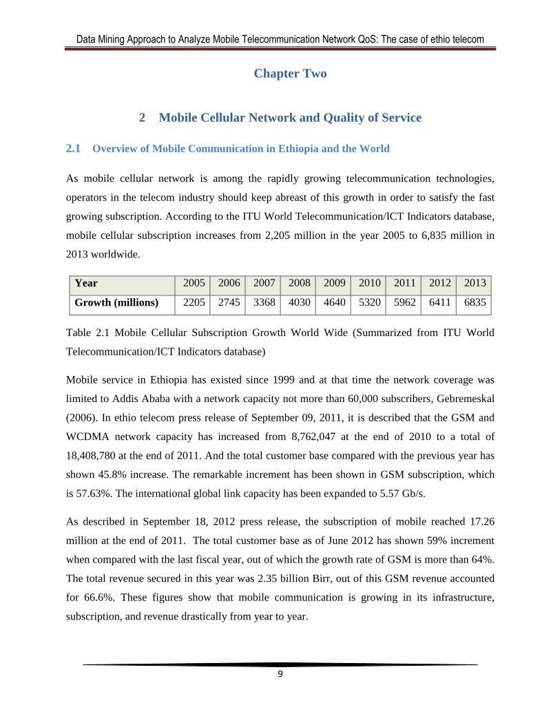
As mobile cellular network is among the rapidly growing telecommunication technologies,
operators in the telecom industry should keep abreast of this growth in order to satisfy the fast
growing subscription. According to the ITU World Telecommunication/ICT Indicators database,
mobile cellular subscription increases from 2,205 million in the year 2005 to 6,835 million in
2013 worldwide.
Year 2005 2006 2007 2008 2009 2010 2011 2012 2013
Growth (millions) 2205 2745 3368 4030 4640 5320 5962 6411 6835
Table 2.1 Mobile Cellular Subscription Growth World Wide (Summarized from ITU World
Telecommunication/ICT Indicators database)
Mobile service in Ethiopia has existed since 1999 and at that time the network coverage was
limited to Addis Ababa with a network capacity not more than 60,000 subscribers, Gebremeskal
(2006). In ethio telecom press release of September 09, 2011, it is described that the GSM and
WCDMA network capacity has increased from 8,762,047 at the end of 2010 to a total of
18,408,780 at the end of 2011. And the total customer base compared with the previous year has
shown 45.8% increase. The remarkable increment has been shown in GSM subscription, which
is 57.63%. The international global link capacity has been expanded to 5.57 Gb/s.
As described in September 18, 2012 press release, the subscription of mobile reached 17.26
million at the end of 2011. The total customer base as of June 2012 has shown 59% increment
when compared with the last fiscal year, out of which the growth rate of GSM is more than 64%.
The total revenue secured in this year was 2.35 billion Birr, out of this GSM revenue accounted
for 66.6%. These figures show that mobile communication is growing in its infrastructure,
subscription, and revenue drastically from year to year.
Data Mining Approach to Analyze Mobile Telecommunication Network QoS: The case of ethio telecom
10
2.2 Standardization Bodies in Mobile Technology
The major standardization bodies that play an important role in defining the specifications for the
mobile technology as discussed in Mishra (2004) are:
ITU (International Telecommunication Union): The ITU, with headquarters in Geneva,
Switzerland, is an international organization within the United Nations, where global
telecom networks and services are coordinated in governments and the private sector.
The ITU-T is one of the three sectors of ITU and produces the quality standards covering
all the fields of telecommunications.
ETSI (European Telecommunication Standard Institute): This body was primarily
responsible for the development of the specifications for the GSM. Owing to the
technical and commercial success of the GSM, this body will also play an important role
in the development of third-generation mobile systems. ETSI mainly develops the
telecommunication standards throughout Europe and beyond.
ARIB (Alliance of Radio Industries and Business): This body is predominant in the
Australasian region and is playing an important role in the development of third-
generation mobile systems. ARIB basically serves as a standards developing organization
for radio technology.
ANSI (American National Standards Institute): ANSI currently provides a forum for over
270 ANSI-accredited standards developers representing approximately 200 distinct
organizations in the private and public sectors. This body has been responsible for the
standards development for the American networks.
3GPP (Third Generation Partnership Project): This body was created to maintain overall
control of the specification design and process for third-generation networks. The result
of the 3GPP work is a complete set of specifications that will maintain the global nature
of the 3G networks.
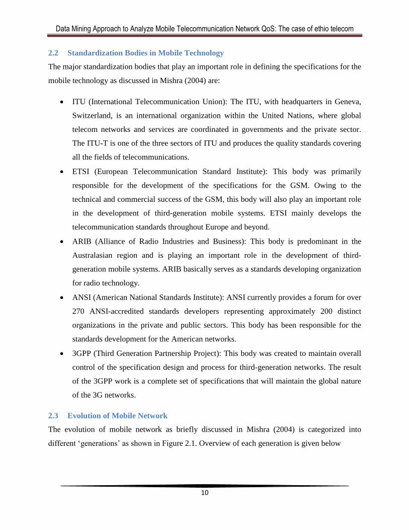
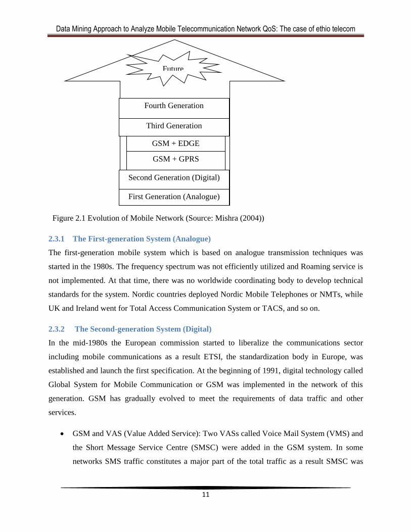
2.3 Evolution of Mobile Network
The evolution of mobile network as briefly discussed in Mishra (2004) is categorized into
different ‗generations‘ as shown in Figure 2.1. Overview of each generation is given below
Data Mining Approach to Analyze Mobile Telecommunication Network QoS: The case of ethio telecom
11
Figure 2.1 Evolution of Mobile Network (Source: Mishra (2004))
2.3.1 The First-generation System (Analogue)
The first-generation mobile system which is based on analogue transmission techniques was
started in the 1980s. The frequency spectrum was not efficiently utilized and Roaming service is
not implemented. At that time, there was no worldwide coordinating body to develop technical
standards for the system. Nordic countries deployed Nordic Mobile Telephones or NMTs, while
UK and Ireland went for Total Access Communication System or TACS, and so on.
2.3.2 The Second-generation System (Digital)
In the mid-1980s the European commission started to liberalize the communications sector
including mobile communications as a result ETSI, the standardization body in Europe, was
established and launch the first specification. At the beginning of 1991, digital technology called
Global System for Mobile Communication or GSM was implemented in the network of this
generation. GSM has gradually evolved to meet the requirements of data traffic and other
services.
GSM and VAS (Value Added Service): Two VASs called Voice Mail System (VMS) and
the Short Message Service Centre (SMSC) were added in the GSM system. In some
networks SMS traffic constitutes a major part of the total traffic as a result SMSC was
First Generation (Analogue)
Second Generation (Digital)
GSM + GPRS
GSM + EDGE
Third Generation
Fourth Generation
Future
Data Mining Approach to Analyze Mobile Telecommunication Network QoS: The case of ethio telecom
12
commercially successful. IN (Intelligent) services are also emerged and made fraud
management and 'pre-paid' services to be created.
GSM and GPRS (General Packet Radio Services): SGSN (Serving GPRS Support Node)
and GGSN (Gateway GPRS Support Node) were added to the existing GSM system to
send packet data on the air-interface. Part of the network handling the packet data is
called the 'packet core network'. This network also contains the IP routers, firewall
servers and DNS (domain name servers) in addition to the SGSN and GGSN. This
enables wireless access to the Internet and the bit rate reaching to 150 kbps optimally.
GSM and EDGE (Enhanced Data rates in GSM Environment): The need to increase the
data rate in the data traffic was done by using more sophisticated coding methods over
the Internet and thus increasing the data rate up to 384 kbps.
2.3.3 Third-generation Networks (WCDMA in UMTS)
Though high volume movement of data was possible in EDGE, still the packet transfer on the air
interface work like a circuit switches call, which results in loss of packet connection in the circuit
switch environment. The inconsistency of network standards around the world was also another
challenge. Hence, it was decided to have a network its design standards are the same globally
and provides services irrespective of technology platform. Thus, 3G also called UMTS
(Universal Terrestrial Mobile System) in Europe, which is ETSI-driven, was born. IMT-2000 is
the ITU-T name for the 3G system. WCDMA is the air-interface technology for the UMTS. The
main components include BS (base station) or node B, RNC (radio network controller) apart
from WMSC (wideband CDMA mobile switching center) and SGSN/GGSN. This platform
offers many Internet based services, along with video phoning, imaging, etc.
2.3.4 Fourth-generation Networks (All-IP)
The fundamental reason for the transition to the All-IP is to have a common platform for all the
technologies that have been developed so far, and to harmonize with user expectations of the
many services to be provided. The fundamental difference between the GSM/3G and All-IP is
that the functionality of the RNC and BSC is now distributed to the BTS and a set of servers and
gateways. This means that this network will be less expensive and data transfer will be much
faster.
Data Mining Approach to Analyze Mobile Telecommunication Network QoS: The case of ethio telecom
13
2.4 Multiple-access Techniques
According to Horak (2007), communication networks adopt the concept of DAMA (Demand -
Assigned Multiple Access). DAMA enables multiple devices to share access to the same network
on a demand basis, that is, first come, first served. There exist a number of techniques for
providing multiple accesses (i.e., access to multiple users) in a wireless network. Those
techniques generally, but not always, are mutually exclusive.
Frequency division is the starting point for all wireless communications because all
communications within a given cell must be separated by frequency to avoid mutual interference.
Frequency Division Multiple Access (FDMA) divides the assigned frequency range into multiple
frequency channels to support multiple conversations. Analog cellular systems employ FDMA.
As discussed in Mishra (2004) the advantage of the FDMA system is that transmission can be
without coordination or synchronization and its constraint is the limited availability of
frequencies.
As mobile communications moved on to the second generation, FDMA was not considered an
effective way for frequency utilization, so time division multiple access (TDMA) was
introduced. TDMA is a digital technique that divides each frequency channel into multiple time
slots, each time slot supports an individual conversation Horak (2007); Mishra (2004).
Code Division Multiple Access (CDMA) is relatively new technology, initially developed for
military applications, has better bandwidth and service quality in congestion and interference
environment. In this technology, every user is assigned a separate code/s depending on the
transaction. One user may have several codes, thus, separation is based on codes than frequency
or time. These codes are very long sequences of bits having a higher bit rate than the original
information. The major advantage of using CDMA is that no plan is needed for frequency re-use,
greater number of channels, effective utilization of bandwidth, and the confidentiality of
information is well protected Horak (2007); Mishra (2004).
2.5 System Capacity
According to Dunlop and Smith (2000), the capacity of a system may be described in terms of
the number of available channels or the number of subscribers that the system will support. The
latter measure assumes that each call has a mean duration and not all of the subscribers will be
Data Mining Approach to Analyze Mobile Telecommunication Network QoS: The case of ethio telecom
14
trying to make a call concurrently. Thus, it is the capacity planning undertaken from the outset
that determines the system capacity. In this regard, Mishra (2004) identifies three essential
parameters required for capacity planning: Estimated traffic, Average antenna height, and
Frequency usage described in short hear after:
2.5.1 Traffic Estimates
Experience developed from studying an existing network and theoretical baselines are crucial for
traffic estimates. Traffic in the network is dependent on two variables: the user communication
rate, which is the amount of traffic generated by the subscriber per unit time and the user
movement, which estimates the dynamic and static mode of network usage. The traffic on this
network is estimated in terms of ‗erlangs‘. One erlang (1Erl) is equivalent to the utilization of a
traffic channel for an hour. Considering that subscribers are speaking for 120 seconds on
average, it is assumed that they will generate 25 mErl of traffic during busy hours. In some
networks this figure will be 35 mErl and 90 s respectively.
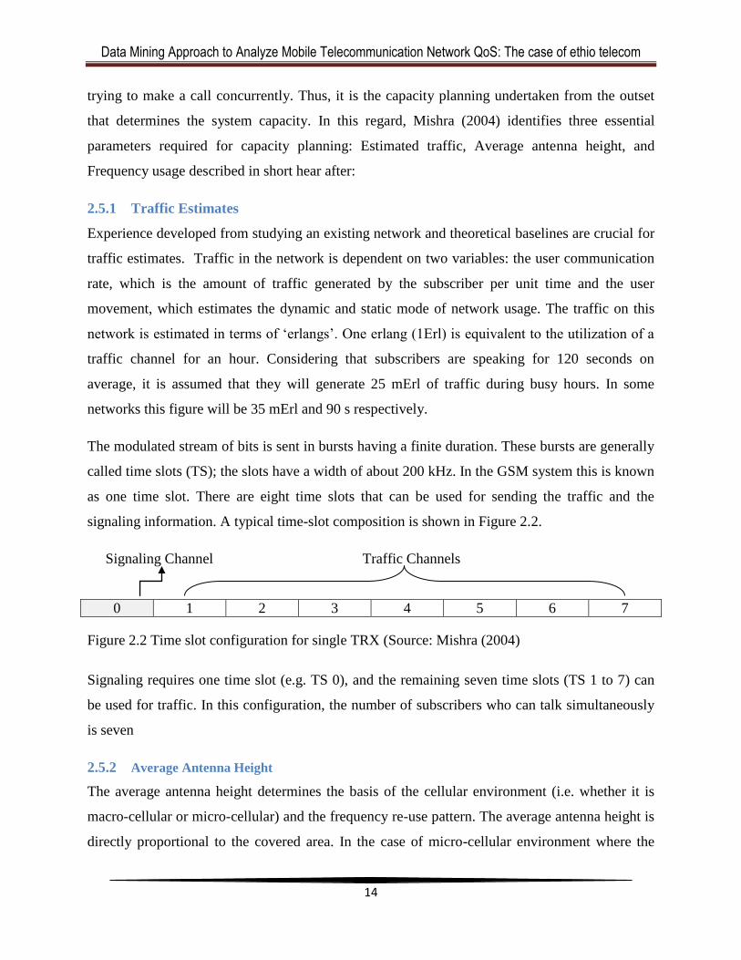
The modulated stream of bits is sent in bursts having a finite duration. These bursts are generally
called time slots (TS); the slots have a width of about 200 kHz. In the GSM system this is known
as one time slot. There are eight time slots that can be used for sending the traffic and the
signaling information. A typical time-slot composition is shown in Figure 2.2.
Signaling Channel Traffic Channels
Figure 2.2 Time slot configuration for single TRX (Source: Mishra (2004)
Signaling requires one time slot (e.g. TS 0), and the remaining seven time slots (TS 1 to 7) can
be used for traffic. In this configuration, the number of subscribers who can talk simultaneously
is seven
2.5.2 Average Antenna Height
The average antenna height determines the basis of the cellular environment (i.e. whether it is
macro-cellular or micro-cellular) and the frequency re-use pattern. The average antenna height is
directly proportional to the covered area. In the case of micro-cellular environment where the
0 1 2 3 4 5 6 7

Data Mining Approach to Analyze Mobile Telecommunication Network QoS: The case of ethio telecom
15
antenna height is low, there is an increase in the number of times the same frequency can be re-
allocated and this will lead to the creation of more cells. The opposite is the case in a macro-
cellular environment where the same frequency can be reallocated fewer times and the coverage
area would be more. These relations are based on the interference analysis of the system as well
as the topography and propagation conditions.
2.5.3 Frequency Usage and Re-use
Frequency usage is a concept related to both coverage and capacity usage and frequency re-use
means how often a frequency can be re-used in the network. According to Dunlop and Smith
(2000), the total number of voice channels depends on the radio spectrum allocated and the
bandwidth of each channel. Based on this number a frequency reuse pattern must be developed
in order to optimally use the channels and this is closely linked with cell size. The following are
among the factors that decide the minimum distance where the same frequencies to be re-used:
i. The number of co-channel cells in the vicinity of the center cell;
ii. The geography of the terrain;
iii. The antenna height;
iv. The transmitted power within each cell
2.6 Constituents of Mobile Networks
Mishra (2004) provides a detailed description about the constituents of a mobile network on each
generation. A condensed description of the 2G, 3G, and 4G is given in the coming paragraphs.
Interested reader may refer this text to have a detailed knowledge on this area.
2.6.1 Second Generation Network
Out of the second-generation mobile systems, GSM is the most widely used. It is divided into
three major parts: base station subsystem, network subsystem, and network management system
as shown in Figure 2.3.
Data Mining Approach to Analyze Mobile Telecommunication Network QoS: The case of ethio telecom
16
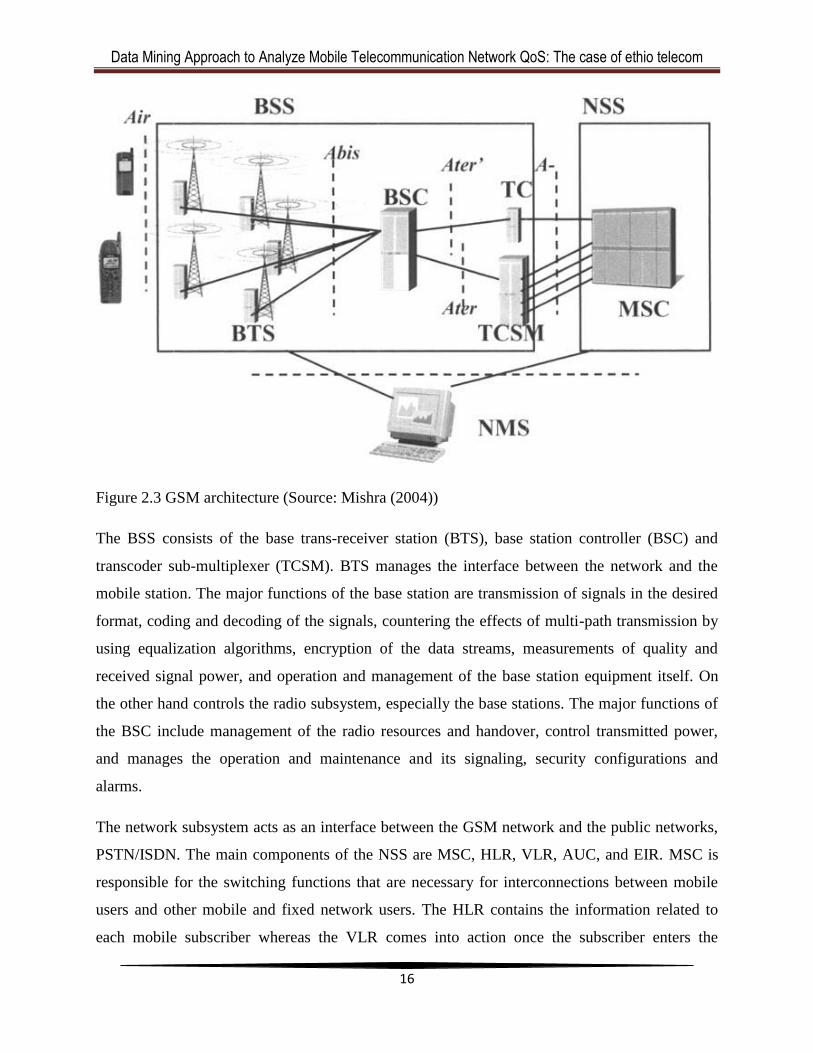
Figure 2.3 GSM architecture (Source: Mishra (2004))
The BSS consists of the base trans-receiver station (BTS), base station controller (BSC) and
transcoder sub-multiplexer (TCSM). BTS manages the interface between the network and the
mobile station. The major functions of the base station are transmission of signals in the desired
format, coding and decoding of the signals, countering the effects of multi-path transmission by
using equalization algorithms, encryption of the data streams, measurements of quality and
received signal power, and operation and management of the base station equipment itself. On
the other hand controls the radio subsystem, especially the base stations. The major functions of
the BSC include management of the radio resources and handover, control transmitted power,
and manages the operation and maintenance and its signaling, security configurations and
alarms.
The network subsystem acts as an interface between the GSM network and the public networks,
PSTN/ISDN. The main components of the NSS are MSC, HLR, VLR, AUC, and EIR. MSC is
responsible for the switching functions that are necessary for interconnections between mobile
users and other mobile and fixed network users. The HLR contains the information related to
each mobile subscriber whereas the VLR comes into action once the subscriber enters the
Data Mining Approach to Analyze Mobile Telecommunication Network QoS: The case of ethio telecom
17
coverage region and it is dynamic in nature. The AUC (or AC) is responsible for controlling
actions in the network. The EIR contains the International Mobile Equipment Identity (IMEI) list
of authorized numbers and allows the IMEI to be verified. Finally the NMS has four major tasks
to perform: network monitoring, network development, network measurements, and fault
management.
2.6.2 Third Generation Network
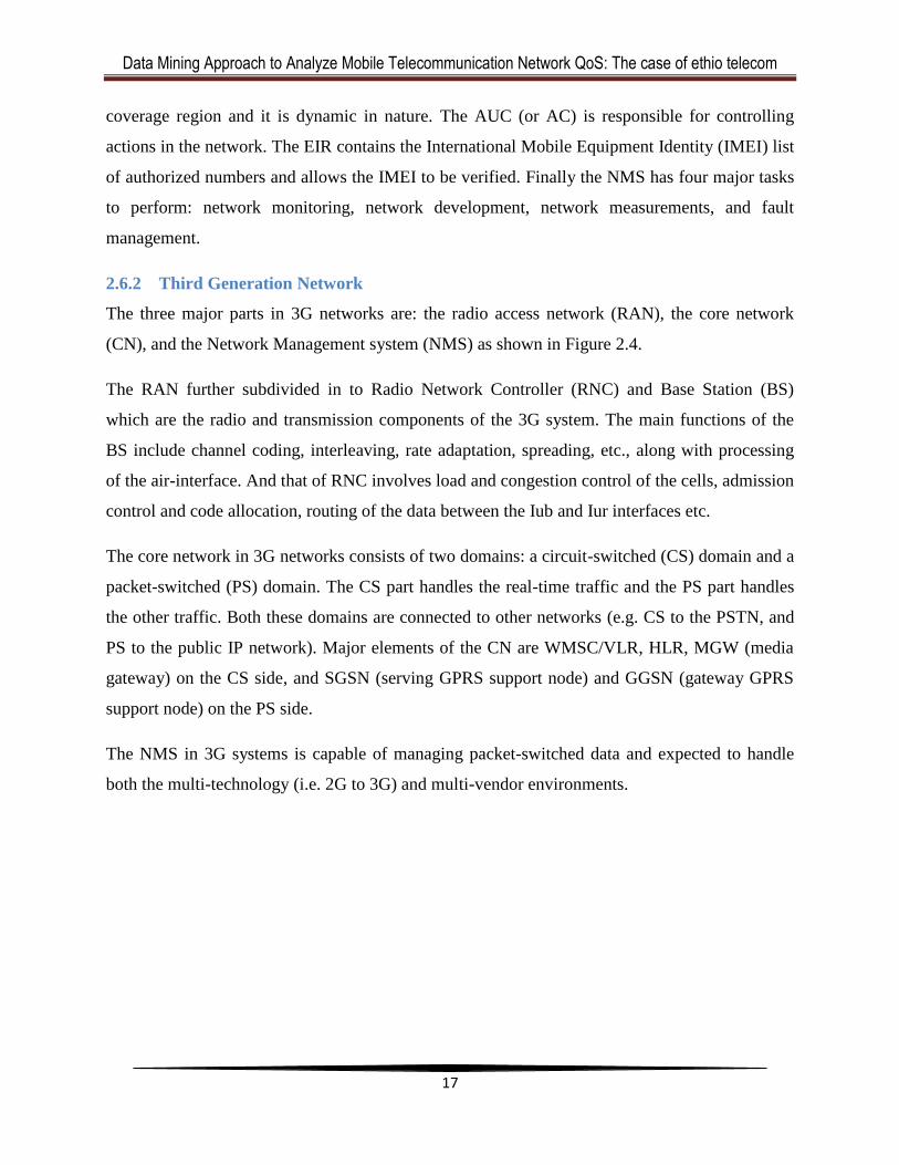
The three major parts in 3G networks are: the radio access network (RAN), the core network
(CN), and the Network Management system (NMS) as shown in Figure 2.4.
The RAN further subdivided in to Radio Network Controller (RNC) and Base Station (BS)
which are the radio and transmission components of the 3G system. The main functions of the
BS include channel coding, interleaving, rate adaptation, spreading, etc., along with processing
of the air-interface. And that of RNC involves load and congestion control of the cells, admission
control and code allocation, routing of the data between the Iub and Iur interfaces etc.
The core network in 3G networks consists of two domains: a circuit-switched (CS) domain and a
packet-switched (PS) domain. The CS part handles the real-time traffic and the PS part handles
the other traffic. Both these domains are connected to other networks (e.g. CS to the PSTN, and
PS to the public IP network). Major elements of the CN are WMSC/VLR, HLR, MGW (media
gateway) on the CS side, and SGSN (serving GPRS support node) and GGSN (gateway GPRS
support node) on the PS side.
The NMS in 3G systems is capable of managing packet-switched data and expected to handle
both the multi-technology (i.e. 2G to 3G) and multi-vendor environments.
Data Mining Approach to Analyze Mobile Telecommunication Network QoS: The case of ethio telecom
18
Figure 2.4 Third generation system (WCDMA) (Source: Mishra (2004))
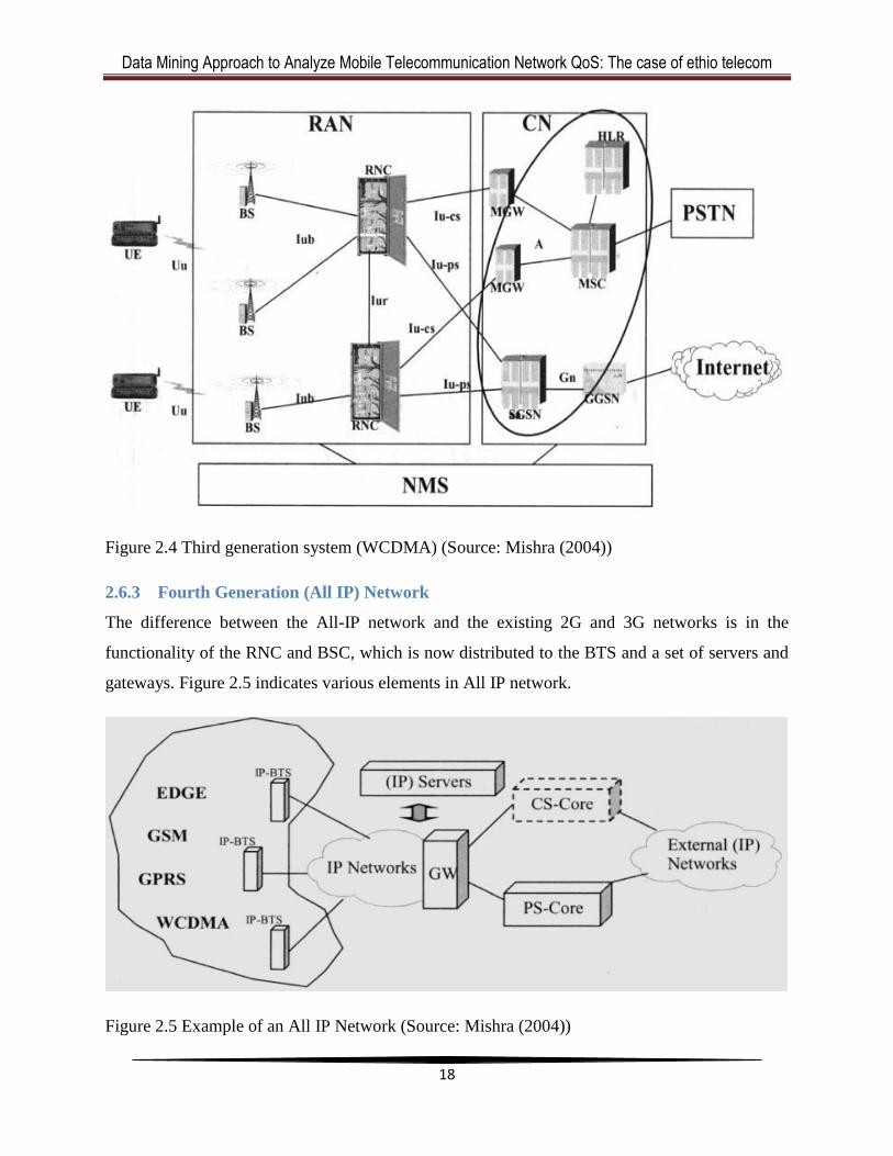
2.6.3 Fourth Generation (All IP) Network
The difference between the All-IP network and the existing 2G and 3G networks is in the
functionality of the RNC and BSC, which is now distributed to the BTS and a set of servers and
gateways. Figure 2.5 indicates various elements in All IP network.
Figure 2.5 Example of an All IP Network (Source: Mishra (2004))
Data Mining Approach to Analyze Mobile Telecommunication Network QoS: The case of ethio telecom
19
IP-BTS: The functionality of the IP BTS in this network is more than the functionality of base
stations seen in the earlier generations; it acts as a mini-RNC/BSC.
(IP) servers: The IP BTS is not capable of performing all the RNC/BSC functions, which are of
network level. These servers handle the signaling between the network elements.
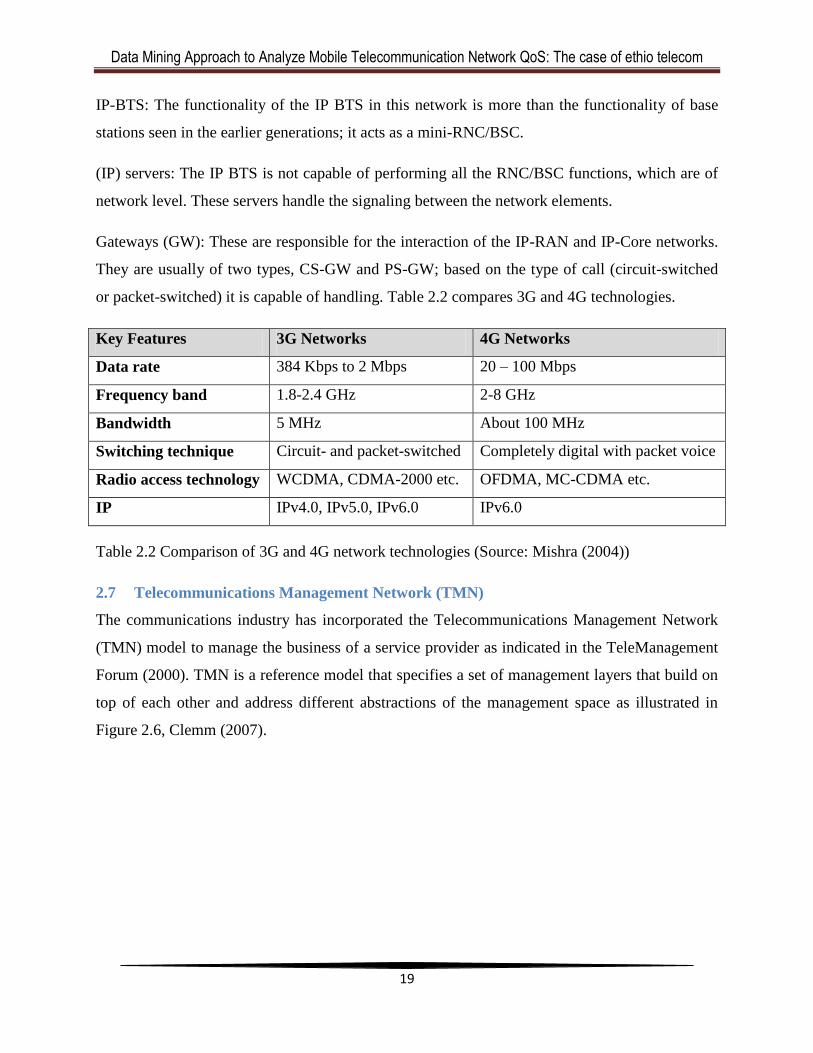
Gateways (GW): These are responsible for the interaction of the IP-RAN and IP-Core networks.
They are usually of two types, CS-GW and PS-GW; based on the type of call (circuit-switched
or packet-switched) it is capable of handling. Table 2.2 compares 3G and 4G technologies.
Key Features 3G Networks 4G Networks
Data rate 384 Kbps to 2 Mbps 20 – 100 Mbps
Frequency band 1.8-2.4 GHz 2-8 GHz
Bandwidth 5 MHz About 100 MHz
Switching technique Circuit- and packet-switched Completely digital with packet voice
Radio access technology WCDMA, CDMA-2000 etc. OFDMA, MC-CDMA etc.
IP IPv4.0, IPv5.0, IPv6.0 IPv6.0
Table 2.2 Comparison of 3G and 4G network technologies (Source: Mishra (2004))
2.7 Telecommunications Management Network (TMN)
The communications industry has incorporated the Telecommunications Management Network
(TMN) model to manage the business of a service provider as indicated in the TeleManagement
Forum (2000). TMN is a reference model that specifies a set of management layers that build on
top of each other and address different abstractions of the management space as illustrated in
Figure 2.6, Clemm (2007).
Data Mining Approach to Analyze Mobile Telecommunication Network QoS: The case of ethio telecom
20
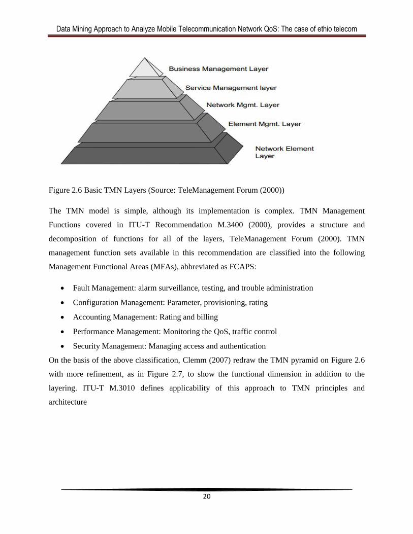
Figure 2.6 Basic TMN Layers (Source: TeleManagement Forum (2000))
The TMN model is simple, although its implementation is complex. TMN Management
Functions covered in ITU-T Recommendation M.3400 (2000), provides a structure and
decomposition of functions for all of the layers, TeleManagement Forum (2000). TMN
management function sets available in this recommendation are classified into the following
Management Functional Areas (MFAs), abbreviated as FCAPS:
Fault Management: alarm surveillance, testing, and trouble administration
Configuration Management: Parameter, provisioning, rating
Accounting Management: Rating and billing
Performance Management: Monitoring the QoS, traffic control
Security Management: Managing access and authentication
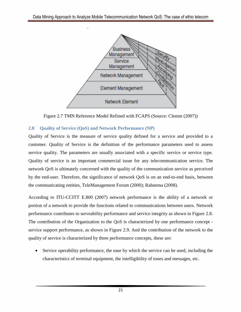
On the basis of the above classification, Clemm (2007) redraw the TMN pyramid on Figure 2.6
with more refinement, as in Figure 2.7, to show the functional dimension in addition to the
layering. ITU-T M.3010 defines applicability of this approach to TMN principles and
architecture
Data Mining Approach to Analyze Mobile Telecommunication Network QoS: The case of ethio telecom
21
Figure 2.7 TMN Reference Model Refined with FCAPS (Source: Clemm (2007))
2.8 Quality of Service (QoS) and Network Performance (NP)
Quality of Service is the measure of service quality defined for a service and provided to a
customer. Quality of Service is the definition of the performance parameters used to assess
service quality. The parameters are usually associated with a specific service or service type.
Quality of service is an important commercial issue for any telecommunication service. The
network QoS is ultimately concerned with the quality of the communication service as perceived
by the end-user. Therefore, the significance of network QoS is on an end-to-end basis, between
the communicating entities, TeleManagement Forum (2000); Rahnema (2008).
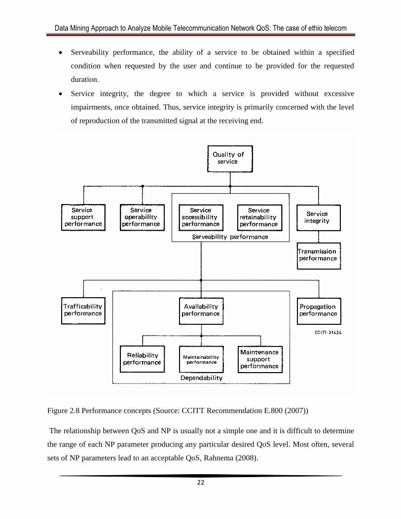
According to ITU-CCITT E.800 (2007) network performance is the ability of a network or
portion of a network to provide the functions related to communications between users. Network
performance contributes to serveability performance and service integrity as shown in Figure 2.8.
The contribution of the Organization to the QoS is characterized by one performance concept -
service support performance, as shown in Figure 2.9. And the contribution of the network to the
quality of service is characterized by three performance concepts, these are:
Service operability performance, the ease by which the service can be used, including the
characteristics of terminal equipment, the intelligibility of tones and messages, etc.
Data Mining Approach to Analyze Mobile Telecommunication Network QoS: The case of ethio telecom
22
Serveability performance, the ability of a service to be obtained within a specified
condition when requested by the user and continue to be provided for the requested
duration.
Service integrity, the degree to which a service is provided without excessive
impairments, once obtained. Thus, service integrity is primarily concerned with the level
of reproduction of the transmitted signal at the receiving end.
Figure 2.8 Performance concepts (Source: CCITT Recommendation E.800 (2007))
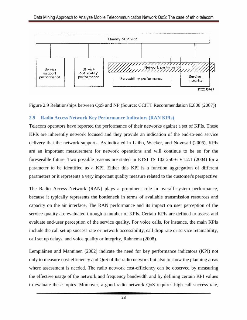
The relationship between QoS and NP is usually not a simple one and it is difficult to determine
the range of each NP parameter producing any particular desired QoS level. Most often, several
sets of NP parameters lead to an acceptable QoS, Rahnema (2008).
Data Mining Approach to Analyze Mobile Telecommunication Network QoS: The case of ethio telecom
23
Figure 2.9 Relationships between QoS and NP (Source: CCITT Recommendation E.800 (2007))
2.9 Radio Access Network Key Performance Indicators (RAN KPIs)
Telecom operators have reported the performance of their networks against a set of KPIs. These
KPIs are inherently network focused and they provide an indication of the end-to-end service
delivery that the network supports. As indicated in Laiho, Wacker, and Novosad (2006), KPIs
are an important measurement for network operations and will continue to be so for the
foreseeable future. Two possible reasons are stated in ETSI TS 102 250-6 V1.2.1 (2004) for a
parameter to be identified as a KPI. Either this KPI is a function aggregation of different
parameters or it represents a very important quality measure related to the customer's perspective
The Radio Access Network (RAN) plays a prominent role in overall system performance,
because it typically represents the bottleneck in terms of available transmission resources and
capacity on the air interface. The RAN performance and its impact on user perception of the
service quality are evaluated through a number of KPIs. Certain KPIs are defined to assess and
evaluate end-user perception of the service quality. For voice calls, for instance, the main KPIs
include the call set up success rate or network accessibility, call drop rate or service retainability,
call set up delays, and voice quality or integrity, Rahnema (2008).
Lempiäinen and Manninen (2002) indicate the need for key performance indicators (KPI) not
only to measure cost-efficiency and QoS of the radio network but also to show the planning areas
where assessment is needed. The radio network cost-efficiency can be observed by measuring
the effective usage of the network and frequency bandwidth and by defining certain KPI values
to evaluate these topics. Moreover, a good radio network QoS requires high call success rate,
Data Mining Approach to Analyze Mobile Telecommunication Network QoS: The case of ethio telecom
24
good voice quality and normal call release. In order to analyze the radio QoS, the KPI values
such as call success rate, handover success rate, dropped call rate and blocking have to be
measured.
The performance of cellular networks is crucial for telecom operators as their main goal is to
keep the subscribers satisfied with the QoS they provide. To achieve the best performance, they
have to monitor and analyze their network continuously. RAN KPIs are among the reports
generated by the network and analyzed to optimize QoS. These raw data are available on the
Network Management System (NMS) on-line database, Kyriazakos and Karetsos (2004), The
KPI data undertaken for this specific research would be extracted from the NMS database of the
operational mobile network of ethio telecom.
2.9.1 Logical Channels
Logical channels occur through the allocation of time slots by physical channels. Consequently
the data of a logical channel is transmitted in the corresponding time slots of the physical
channel. During this process, logical channels can occupy a part of the physical channel or even
the entire channel. The GSM recommendations define several logical channels for signaling on
the basis of this principle, dividing them into two main groups: traffic channels and control
channels, as described in Kyriazakos and Karetsos (2004):
Traffic channels (TCH) are logical channels over which user information are exchanged
between mobile users during a connection. Speech and data are digitally transmitted on these
channels using different coding methods. It includes full rate traffic channel and half rate traffic
channel.
Control channels (CCH): Control information is used for signaling and for system control.
Typical signaling tasks include the signaling for establishing, maintaining and releasing traffic
channels, for mobility management and access control to radio channels. Control information is
transmitted over so-called control channels (CCH). Three groups of control channels were
defined in GSM:
Broadcast control channel (BCCH) which includes frequency correction channel (FCCH)
and synchronization channel (SCH) as a sub class.
Data Mining Approach to Analyze Mobile Telecommunication Network QoS: The case of ethio telecom
25
Common control channel (CCCH) which includes Paging channel (PCH), Random
access channel (RACH), and Access grant channel (AGCH) as a sub class.
Dedicated control channel (DCCH) which includes Stand-alone dedicated control
channel (SDCCH), Slow associated dedicated control channel (SACCH), and Fast
associated dedicated control channel (FACCH) as a sub class.
Kyriazakos et al. find out that the logical channels that are primarily used in todays, mainly,
voice traffic in cellular networks are the TCH (Traffic Channel) and the SDCCH (Stand-alone
dedicated control channel) often referred as signaling channel. This paper also focuses on the
KPI data of these two logical channels and handover.
2.9.2 Performance Measurement
As stated in Gómez and Sánchez (2005), performance measurement in the telecom world is
usually defined in terms of accessibility, retainability and quality. Accessibility can be defined
with the blocked calls, retainability with the dropped calls, and the quality with speech frame
error rate. All these measured can be taken at the radio level (i.e. BSS) and easily translated into
service quality.
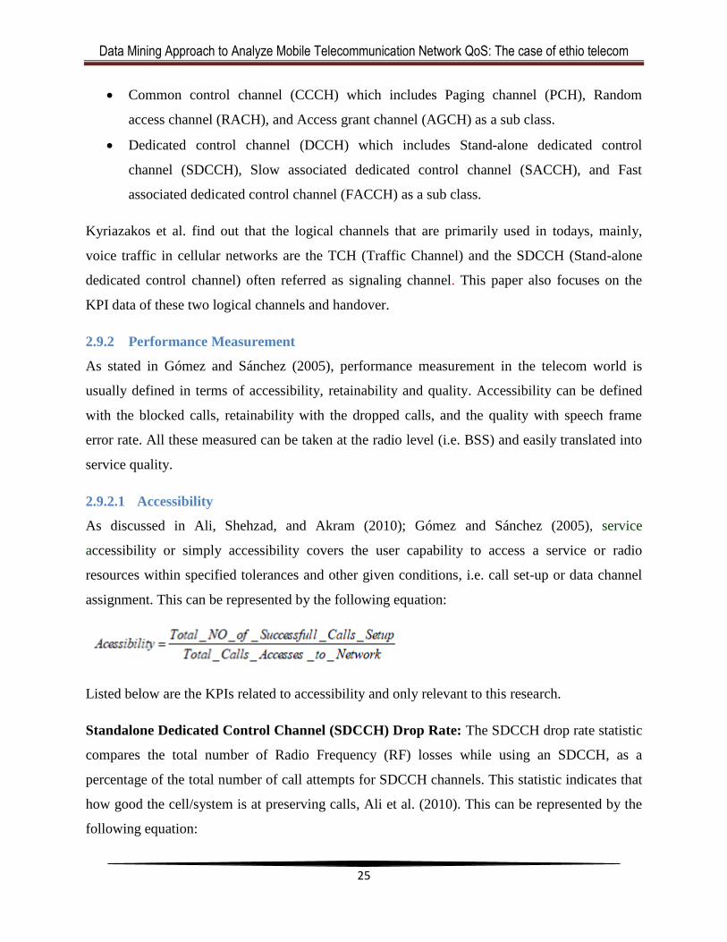
2.9.2.1 Accessibility
As discussed in Ali, Shehzad, and Akram (2010); Gómez and Sánchez (2005), service
accessibility or simply accessibility covers the user capability to access a service or radio
resources within specified tolerances and other given conditions, i.e. call set-up or data channel
assignment. This can be represented by the following equation:
Listed below are the KPIs related to accessibility and only relevant to this research.
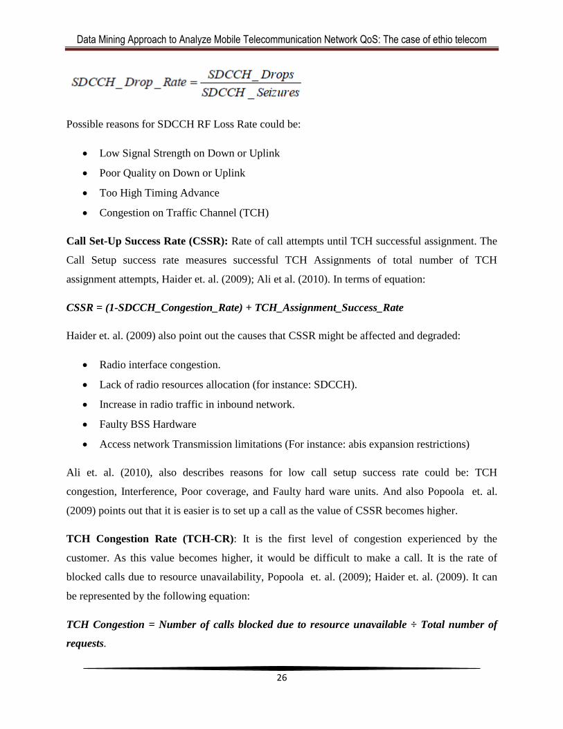
Standalone Dedicated Control Channel (SDCCH) Drop Rate: The SDCCH drop rate statistic
compares the total number of Radio Frequency (RF) losses while using an SDCCH, as a
percentage of the total number of call attempts for SDCCH channels. This statistic indicates that
how good the cell/system is at preserving calls, Ali et al. (2010). This can be represented by the
following equation:
Data Mining Approach to Analyze Mobile Telecommunication Network QoS: The case of ethio telecom
26
Possible reasons for SDCCH RF Loss Rate could be:
Low Signal Strength on Down or Uplink
Poor Quality on Down or Uplink
Too High Timing Advance
Congestion on Traffic Channel (TCH)
Call Set-Up Success Rate (CSSR): Rate of call attempts until TCH successful assignment. The
Call Setup success rate measures successful TCH Assignments of total number of TCH
assignment attempts, Haider et. al. (2009); Ali et al. (2010). In terms of equation:
CSSR = (1-SDCCH_Congestion_Rate) + TCH_Assignment_Success_Rate
Haider et. al. (2009) also point out the causes that CSSR might be affected and degraded:
Radio interface congestion.
Lack of radio resources allocation (for instance: SDCCH).
Increase in radio traffic in inbound network.
Faulty BSS Hardware
Access network Transmission limitations (For instance: abis expansion restrictions)
Ali et. al. (2010), also describes reasons for low call setup success rate could be: TCH
congestion, Interference, Poor coverage, and Faulty hard ware units. And also Popoola et. al.
(2009) points out that it is easier is to set up a call as the value of CSSR becomes higher.
TCH Congestion Rate (TCH-CR): It is the first level of congestion experienced by the
customer. As this value becomes higher, it would be difficult to make a call. It is the rate of
blocked calls due to resource unavailability, Popoola et. al. (2009); Haider et. al. (2009). It can
be represented by the following equation:
TCH Congestion = Number of calls blocked due to resource unavailable ÷ Total number of
requests.
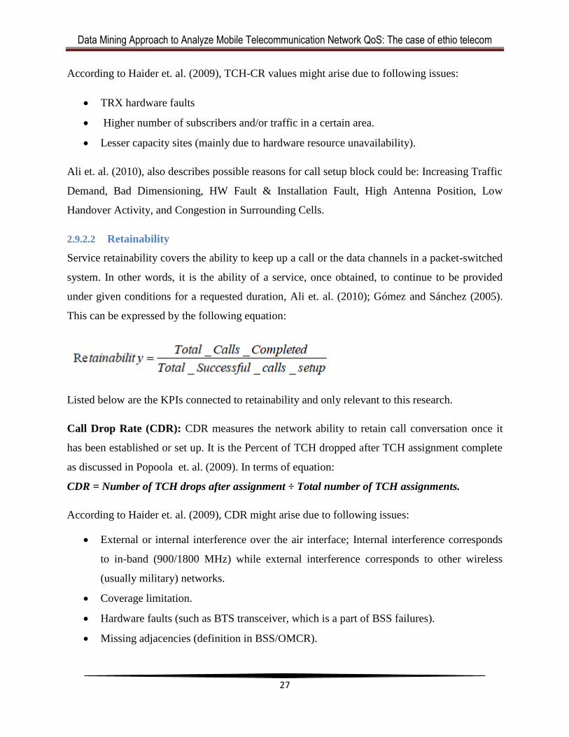
Data Mining Approach to Analyze Mobile Telecommunication Network QoS: The case of ethio telecom
27
According to Haider et. al. (2009), TCH-CR values might arise due to following issues:
TRX hardware faults
Higher number of subscribers and/or traffic in a certain area.
Lesser capacity sites (mainly due to hardware resource unavailability).
Ali et. al. (2010), also describes possible reasons for call setup block could be: Increasing Traffic
Demand, Bad Dimensioning, HW Fault & Installation Fault, High Antenna Position, Low
Handover Activity, and Congestion in Surrounding Cells.
2.9.2.2 Retainability
Service retainability covers the ability to keep up a call or the data channels in a packet-switched
system. In other words, it is the ability of a service, once obtained, to continue to be provided
under given conditions for a requested duration, Ali et. al. (2010); Gómez and Sánchez (2005).
This can be expressed by the following equation:
Listed below are the KPIs connected to retainability and only relevant to this research.
Call Drop Rate (CDR): CDR measures the network ability to retain call conversation once it
has been established or set up. It is the Percent of TCH dropped after TCH assignment complete
as discussed in Popoola et. al. (2009). In terms of equation:
CDR = Number of TCH drops after assignment ÷ Total number of TCH assignments.
According to Haider et. al. (2009), CDR might arise due to following issues:
External or internal interference over the air interface; Internal interference corresponds
to in-band (900/1800 MHz) while external interference corresponds to other wireless
(usually military) networks.
Coverage limitation.
Hardware faults (such as BTS transceiver, which is a part of BSS failures).
Missing adjacencies (definition in BSS/OMCR).
Data Mining Approach to Analyze Mobile Telecommunication Network QoS: The case of ethio telecom
28
Ali et. al. (2010), also describes some possible reasons for TCH-DCR could be: low signal
strength on down or uplink, lack of best server, congestion in neighboring cells, battery flaw,
poor quality on down or uplink, too high timing advance, antenna problems, low BTS output
power, missing neighboring cell definitions, unsuccessful outgoing and incoming handover.
Handover Success Rate (HOSR): The handover success rate shows the percentage of
successful handovers of all handover attempts. A handover attempt is when a handover
command is sent to the mobile, Ali et. al. (2010). In other words, it is the rate of successful
handovers (intercell + intracell). In terms of equation:
HOSR = No of successful [intercell + intracell] HO Attempt ÷Total number of HO requests.
Haider et. al. (2009) discuss the issues that HOSR might be affected as:
Interference (either external or internal) over the air interface.
Missing adjacencies.
Hardware faults (such as BTS transceiver, which is a part of BSS failures).
Location area code (LAC) boundaries wrongly planned and/or defined (where Location
area represents a cluster of cells).
Coverage limitation.
Ali et. al. (2010), also describes the possible reasons for poor handover success rate could be:
congestion, bad antenna installation, the mobile station (MS) measures signal strength of another
co-or- adjacent cell than presumed, and incorrect handover relations..
2.9.2.3 Connection Quality
Connection quality or service integrity is a measurement of how good the connection or how the
data service is performing. It is subjected to constant changes in response to increasing coverage
and capacity. The way to measure the quality will depend on the type of service and the
availability of measurement in the network. In a telephone network, voice quality is an indicator
of end-to-end speech transmission or connection quality. However, there is a clear limitation to
provide user perspective of the quality from network measurements. Depending on the services,
different performance indicators will be available, Popoola et. al. (2009); Gómez and Sánchez
(2005).
Data Mining Approach to Analyze Mobile Telecommunication Network QoS: The case of ethio telecom
29
Chapter Three
3 Data Mining and Knowledge Discovery
3.1 Basic Concepts
Complex and huge amount of data is generated and captured in every aspect of the industry such
as marketing, insurance, finance, health, telecommunication, etc. However it is difficult for a
human being to manually collect and process these data. This vast amount of data should be
baked up on computerization technology to create a valuable and interesting knowledge, which
brought data mining technology in to existence.
As indicated in Gorunescu (2011), the notion of data mining has emerged in many industries
since 1990s as a process of ―mining‖ data from the academic field for an intended purpose. Han,
Kamber, and Pei (2011) discussed the term data mining as ―the process of discovering interesting
patterns and knowledge from large amounts of data. The data sources can include databases, data
warehouses, the Web, other information repositories, or data that are streamed into the system
dynamically‖ (P.18). There are also other terms synonyms to data mining such as knowledge
mining from data, knowledge extraction, data or pattern analysis, data archaeology, and data
dredging.
As discussed in Gorunescu (2011); Han et. al. (2011), data mining is a multidisciplinary field of
information technology that adopts the techniques and terminologies from various disciplines
such as Artificial Intelligence, Statistics, Database Systems, Data Warehouse, Information
Retrieval, Machine Learning, Applications, Pattern Recognition, Visualization, Algorithms, and
High Performance Computing.
Knowledge Discovery in Databases (KDD) is an automatic, exploratory analysis and modeling
of large data repositories as well as the organized process of identifying crucial knowledge from
large and complex data sets. Data Mining (DM) is the critical task in the KDD process involving
the selection of algorithms that fits the data exploration task, development of model and
discovery of previously unknown patterns. The model can be used to visualize the data generally
Data Mining Approach to Analyze Mobile Telecommunication Network QoS: The case of ethio telecom
30
and to analyze, predict, group, associate, formulate rules… etc. specifically, Maimon and Rokach
(2010).
The move towards offering wide range of contemporary services such as cellular phone, smart
phone, Internet access, email, text messages, images, computer and web data transmissions, and
other data traffic made the telecommunications industry to handle huge and complex data. This
has made the application of data mining mandatory in the area for the accomplishment of many
tasks such as detect fraudulent activities, efficient resource utilization, understand business
dynamics, understand customers, and improve service quality which is in line with this study,
Han et. al. (2011).
3.2 Data Mining Tasks
Functionalities of data mining specify the kinds of patterns found in data mining tasks that can be
generally classified into two categories, descriptive and predictive. Although the boundaries
between prediction and description are not sharp in such a way that some of the predictive
models can be descriptive, to the degree that they are understandable, and vice versa, the
distinction is useful to understand the overall discovery goal. The relative importance of
prediction and description is specific to each data-mining application as the goals is achieved
using a variety of particular data-mining methods, Fayyad, Piatetsky, Shapiro, and Smyth
(1996b); Han et. al. (2011).
3.2.1 Predictive Methods
Predictive mining tasks perform induction on the current data in order to make prediction which
is often referred to as supervised data mining. Moreover, prediction involves using some
variables or fields in the database to predict the values of unknown or future values of other
variables through the application of classification, regression, biases/anomalies detection… etc.
Kumar, Tan, Steinbach (2001); Fayyad et. al. (1996b); Han et. al. (2011); Gorunescu (2011);
Maimon and Rokach (2010). Basic prediction methods are described in the coming paragraphs as
discussed by different scholars.
3.2.1.1 Classification
The natural process of classification where human mind organizes its knowledge differs from the
classification in the context of data mining by the concept of taxonomy. The word ‗Taxonomy‘ is
Data Mining Approach to Analyze Mobile Telecommunication Network QoS: The case of ethio telecom
31
made up of two Greece words ‗tassein = classify‘ and ‗nomos = science law‘, appeared first as
the science of classifying living organisms (alpha taxonomy). However, it is developed latter as
the science of classification in general, including the principles of classification (taxonomic
schemes) too. Thus, the taxonomic or classification is the process of categorizing a specific
object (concept) based on the respective object (concept) properties, Gorunescu (2011).
Han et. al. (2011) defines classification as ―a form of data analysis that extracts models
describing important data classes. Such models called classifiers, predict categorical (discrete,
unordered) class labels‖ (p.271). The book also discusses data classification as a two-step
process that comprises model construction and model application to predict class labels for a
given data. The first one is a learning step where the classification algorithm learns from the
training set that contains a predetermined class label to build the classifier. The second one is a
classification step where the model is applied to classify those data whose class label is unknown
or previously unseen data different from the training set providing that the predictive accuracy of
the model is acceptable. Classification has various applications such as fraud detection, target
marketing, performance prediction, manufacturing, and medical diagnosis.
Gorunescu (2011) also describe the most widely used classification methods as follows:
Decision/classification trees;
Bayesian classifiers/Naive Bayes classifiers;
Neural networks;
Statistical analysis;
Genetic algorithms;
Rough sets;
k-nearest neighbor classifier;
Rule-based methods;
Memory based reasoning;
Support vector machines.
3.2.1.2 Regression
As indicated in Gorunescu (2011), statistically, regression analysis means the mathematical
model which relates the values of a given variable (response/outcome/dependent variable) with
Data Mining Approach to Analyze Mobile Telecommunication Network QoS: The case of ethio telecom
32
the values of other variables (predictor/independent variables). Regression analysis can be used
to determine the quantitative relationship among multiple variables and to forecast the values of
a variable on the basis of the values of other variables.
Kumar et al. (2001) clearly discussed the regression problem in relation with classification
problem. Each record or instance or example in classification is represented by a tuple (x, y),
where x is the set of explanatory variables associated with the object and y is the object‘s class
label. The attributes x1, x2, ・ ・ ・ xk ∈ x can be discrete or continuous however the class label
y must be a discrete variable its value is chosen from a finite set {y1, y2, ・ ・ ・ yc}. If y is a
continuous variable, then this problem is known as regression.
In the context of data mining regression analysis has various applications such as in commerce to
predict the dependent variable sales amounts of new product based on the independent variable
advertising expenditure; in meteorology to predict the dependent variables wind velocities and
directions as a function of temperature, humidity, air pressure, etc.; in stock exchange for time
series prediction of stock market indices (trend estimation); in medicine to visualize the effect of
parental birth weight/height on the dependent variable infant birth weight/height, Gorunescu
(2011).
3.2.1.3 Time series Analysis
Time series data are records accumulated over time and they contains the large fraction of the
world‘s supply of data For example, a company‘s sales, a customer‘s credit card transactions,
and stock prices are all time series data. Such data can be viewed as objects with an attribute
time. The objects are the snapshots of entities with values that change over time, Maimon and
Rokach (2010); Sumathi and Sivanandam (2006).
According to Esling and Agon (2012), a time-series T is an ordered sequence of n real-valued
variables which can be expressed as:
T = (t1. . . tn) , ti ∈ R.
And also a time series can be considered as the result of observation in a certain process where
values are collected from the measurement at uniformly spaced time instants and according to a
Data Mining Approach to Analyze Mobile Telecommunication Network QoS: The case of ethio telecom
33
given sampling rate. Thus, a time series is a set of contiguous time instants its series being
univariate or multivariate.
Maimon and Rokach (2010) also indicate the major tasks of time series in data mining are:
indexing, clustering, classification, prediction, summarization, anomaly detection, and
segmentation.
3.2.1.4 Anomaly Detection
As described in Gorunescu (2011), terms like anomaly, extreme value, or outlier are somewhat
equivalent and refer to a value which is found very far from the rest of data, and represent an
isolated point of the dataset. In other words, they are infrequently observed data points which do
not follow the distribution of the rest of the data.
Anomaly detection identifies data points that are different from the rest of the points in the data
set. Thus, anomaly detection techniques can be applied to detect network intrusions and to
predict fraudulent credit card transactions. Approaches to anomaly detection are based on
statistics or based on distance or graph-theoretic notions, Kumar et. al. (2001).
3.2.2 Descriptive Methods
Descriptive mining tasks characterize properties of the data in a target data set. It focuses on
finding human-interpretable patterns describing the underlying relationships in the data.
Descriptive methods reveal patterns in data through the application of clustering, association
rules, sequential patterns …etc. Moreover descriptive data mining includes the unsupervised and
visualization aspects of data mining, Fayyad et. al. (1996b); Kumar et. al. (2001); Gorunescu
(2011); Maimon and Rokach (2010).
3.2.2.1 Clustering
Unlike classification and prediction, which analyze class-labeled data objects, clustering
analyzes data objects that do not have class label. The class labels are not present in the training
data because they are not known so that clustering can be used to generate such labels. The
objects are clustered or grouped with the aim of maximizing the intra class similarity and
minimizing the interclass similarity. That is, objects within a cluster have high similarity in
comparison to one another, but very dissimilar to objects in other clusters, Han and Kamber
(2006). Thus, clustering can be defined as the process of grouping a collection of patterns into

Data Mining Approach to Analyze Mobile Telecommunication Network QoS: The case of ethio telecom
34
distinct segments or clusters based on a suitable notion of closeness or similarity among these
patterns.
According to Ye (2003), approaches to clustering are broadly classified in to two, these are:
Partitional methods partition the data set into k clusters, the problem being how to determine
the ―best‖ value for k. This can be done by guesswork, by application requirements, or by
running the clustering algorithm several times with different values of k and selecting one of the
solutions based on a suitable evaluation criterion. These algorithms were popular long before the
emergence of data mining. The two most popular representatives are the k-means algorithm and
the k-median algorithm.
Hierarchical methods can be of two types, agglomerative or bottom-up and divisive or top-
down approaches.
The bottom-up approach starts with each object forming a separate group and successively
merges these objects or groups which are closest according to some distance measure, until a
termination condition is satisfied. The distance between two clusters can be measured as the
distance between the closest pair, the farthest pair, or an average among all pairs and the result of
these measures could be a single link, complete link, or average link. Single link is the most
efficient however; it tends to give large clusters and is sensitive to noise. Complete link and
average link methods yield more compact clusters even though they are computationally
expensive.
The top-down approach starts with all the objects in the same cluster. Each successive iteration
result in a cluster to split into smaller clusters according to some measure until a termination
condition is satisfied. Divisive methods are less popular.
3.2.2.2 Association rules
Association rule mining results a set of dependence rules that predict the occurrence of a variable
given the occurrences of other variables. For instance it can be used to identify products often
purchased together; a task referred to as market basket analysis. As indicated in Han and Kamber
(2006), rule interestingness is measured by rule support which reflects usefulness of the
discovered rule and confidence which reflect certainty of the discovered rules.
Data Mining Approach to Analyze Mobile Telecommunication Network QoS: The case of ethio telecom
35
In general, association rule mining can be regarded as a two-step process that involves finding all
frequent item sets, and generating strong association rules from these frequent item sets.
Gorunescu (2011) discussed some popular algorithms in association rule discovery:
A priori algorithm, proposed by Rakesh Agrawal and Ramakrishnan Srikant, being
considered the best-known algorithm to mine association rules
FP-growth (frequent pattern growth) algorithm, proposed by Jiawei Han, Jian Pei,
Yiwen Yin, and Runying Mao
ECLAT (Equivalence Class Clustering and Bottom-up Lattice Traversal), proposed by
Mohammed Javeed Zaki, Srinivasan Parthasarathy, Mitsunori Ogihara, Wei Li
3.2.2.3 Sequential patterns
In sequential pattern mining, frequently occurring ordered events or subsequences are captured
as patterns, the order of occurrence and the value of the events being important. According to
Sumathi and Sivanandam (2006), sequential pattern mining can be applied to investigate changes
in customer consumption or loyalty and suggest adjustments on the pricing and variety of goods
in order to retain existing customers and attract new customers.
Moreover, Gorunescu (2011) discussed some real-life situations where sequential pattern
techniques are employed:
In supermarket, analysis of large database containing sequence of commercial
transactions to streamlining the sale.
In medicine, when diagnosing a disease, symptoms are record on each day and analyzed
in real time to discover sequential patterns for that disease.
In Meteorology, discovering patterns in global climate change such as global warming,
discovering the possibility of occurrence of hurricanes, tsunamis, etc., based on
previously captured events.
3.3 Challenges of Data Mining
Many scholars conduct different studies in order to identify the challenges in data mining.
According to (Fayyad et al. 1996c), the data mining research community often challenged in
developing methods that adopt data mining algorithms for real-world databases . One of the
Data Mining Approach to Analyze Mobile Telecommunication Network QoS: The case of ethio telecom
36
characteristics of real-world databases is huge volume of data that results in several challenges
such as:
Computing complexity: Most algorithms have a computational complexity greater than
linear, if they are applied on a database containing large number of attributes or tuples,
there would be a significant execution time.
Poor classification accuracy due to difficulties in finding the correct classifier as the
search space increases.
Storage problems: The main memory is not capable of storing the training dataset so that
most machine learning algorithms use secondary storage.
Kumar et al. (2001) also indicates several important challenges in applying data mining
techniques to large data sets:
Scalability: Scalable techniques are needed to handle the huge datasets created now days.
Dimensionality: Due to the ―curse of dimensionality‖ in some application domains, the number
of dimensions (or attributes of a record) of the data can be very large, which makes it difficult to
analyze.
Complex Data: More complicated types of structured and semi-structured data have been
generated and captured in recent years. The data analysis techniques should also be modified to
handle the complex nature of such data.
Data Quality: Many data sets have problems with data quality, e.g., erroneous or inexact values,
or missing values. Hence, there is a need for data mining techniques that can perform well even
in such type of problematic situations or with reduced quality of data.
Yang and Wu (2006) also identify 10 challenging problems in data mining research that are
sampled from a small segment of community. These are:
Developing a unifying theory of data mining
Scaling up for high dimensional data and high speed data streams
Mining sequence data and time series data
Mining complex knowledge from complex data

Data Mining Approach to Analyze Mobile Telecommunication Network QoS: The case of ethio telecom
37
Data mining in a network setting
Distributed data mining and mining multi-agent data
Data mining for biological and environmental problems
Data Mining process-related problems
Security, privacy and data integrity
Dealing with non-static, unbalanced and cost-sensitive data
Each ranked important problem in data mining research is discussed in a great detail in the study
for the interested reader.
3.4 Data Mining Process Models
As there are many types of data mining process models, there is no much difference among the
various steps since most of them are interrelated. One could follow a model that fits the specific
data mining project under study. In the article by Yang and Wu (2006), one of the 10 challenging
problems to be solved in data mining research is Data Mining Process-Related Problems.
Important topics exist in improving data-mining tools and processes through automation, as
suggested by several researchers. Specific issues include how to automate the composition of
data mining operations and building a methodology into data mining systems to help users avoid
many data mining mistakes.
As described in Pressman (2005), a process model can be defined as a set of framework activities
and tasks including inputs and outputs in every task to accomplish the desired job. As indicated
in Tyrrell (2000), the following characteristics are crucial for a good process model:
Effective, produce the right product.
Maintainable, the problems should be identified quickly and easily in case of faults.
Predictable, plans are used as the basis for allocating resources: both time and people.
Repeatable, replicable irrespective of specific team and project.
Quality, the product fitness for its purpose.
Improvable, process needs further improvement.
Traceable, easy follow up of the project status..
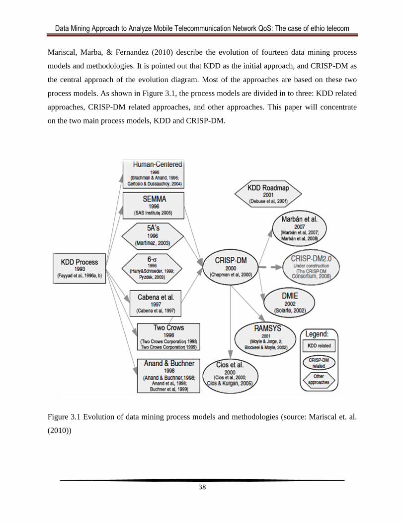
Data Mining Approach to Analyze Mobile Telecommunication Network QoS: The case of ethio telecom
38
Mariscal, Marba, & Fernandez (2010) describe the evolution of fourteen data mining process
models and methodologies. It is pointed out that KDD as the initial approach, and CRISP-DM as
the central approach of the evolution diagram. Most of the approaches are based on these two
process models. As shown in Figure 3.1, the process models are divided in to three: KDD related
approaches, CRISP-DM related approaches, and other approaches. This paper will concentrate
on the two main process models, KDD and CRISP-DM.
Figure 3.1 Evolution of data mining process models and methodologies (source: Mariscal et. al.
(2010))
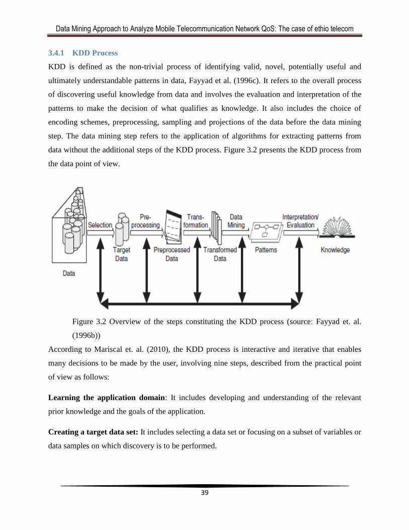
Data Mining Approach to Analyze Mobile Telecommunication Network QoS: The case of ethio telecom
39
3.4.1 KDD Process
KDD is defined as the non-trivial process of identifying valid, novel, potentially useful and
ultimately understandable patterns in data, Fayyad et al. (1996c). It refers to the overall process
of discovering useful knowledge from data and involves the evaluation and interpretation of the
patterns to make the decision of what qualifies as knowledge. It also includes the choice of
encoding schemes, preprocessing, sampling and projections of the data before the data mining
step. The data mining step refers to the application of algorithms for extracting patterns from
data without the additional steps of the KDD process. Figure 3.2 presents the KDD process from
the data point of view.
Figure 3.2 Overview of the steps constituting the KDD process (source: Fayyad et. al.
(1996b))
According to Mariscal et. al. (2010), the KDD process is interactive and iterative that enables
many decisions to be made by the user, involving nine steps, described from the practical point
of view as follows:
Learning the application domain: It includes developing and understanding of the relevant
prior knowledge and the goals of the application.
Creating a target data set: It includes selecting a data set or focusing on a subset of variables or
data samples on which discovery is to be performed.
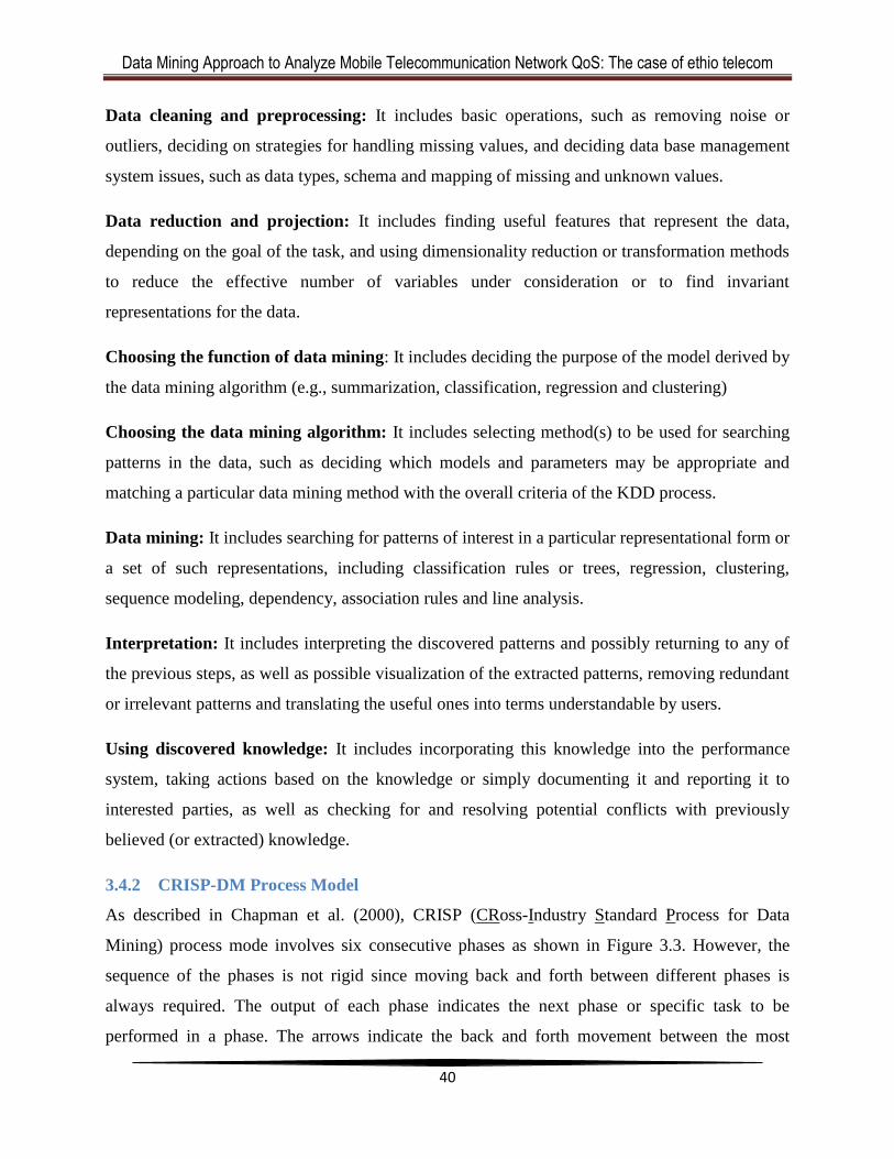
Data Mining Approach to Analyze Mobile Telecommunication Network QoS: The case of ethio telecom
40
Data cleaning and preprocessing: It includes basic operations, such as removing noise or
outliers, deciding on strategies for handling missing values, and deciding data base management
system issues, such as data types, schema and mapping of missing and unknown values.
Data reduction and projection: It includes finding useful features that represent the data,
depending on the goal of the task, and using dimensionality reduction or transformation methods
to reduce the effective number of variables under consideration or to find invariant
representations for the data.
Choosing the function of data mining: It includes deciding the purpose of the model derived by
the data mining algorithm (e.g., summarization, classification, regression and clustering)
Choosing the data mining algorithm: It includes selecting method(s) to be used for searching
patterns in the data, such as deciding which models and parameters may be appropriate and
matching a particular data mining method with the overall criteria of the KDD process.
Data mining: It includes searching for patterns of interest in a particular representational form or
a set of such representations, including classification rules or trees, regression, clustering,
sequence modeling, dependency, association rules and line analysis.
Interpretation: It includes interpreting the discovered patterns and possibly returning to any of
the previous steps, as well as possible visualization of the extracted patterns, removing redundant
or irrelevant patterns and translating the useful ones into terms understandable by users.
Using discovered knowledge: It includes incorporating this knowledge into the performance
system, taking actions based on the knowledge or simply documenting it and reporting it to
interested parties, as well as checking for and resolving potential conflicts with previously
believed (or extracted) knowledge.
3.4.2 CRISP-DM Process Model
As described in Chapman et al. (2000), CRISP (CRoss-Industry Standard Process for Data
Mining) process mode involves six consecutive phases as shown in Figure 3.3. However, the
sequence of the phases is not rigid since moving back and forth between different phases is
always required. The output of each phase indicates the next phase or specific task to be
performed in a phase. The arrows indicate the back and forth movement between the most
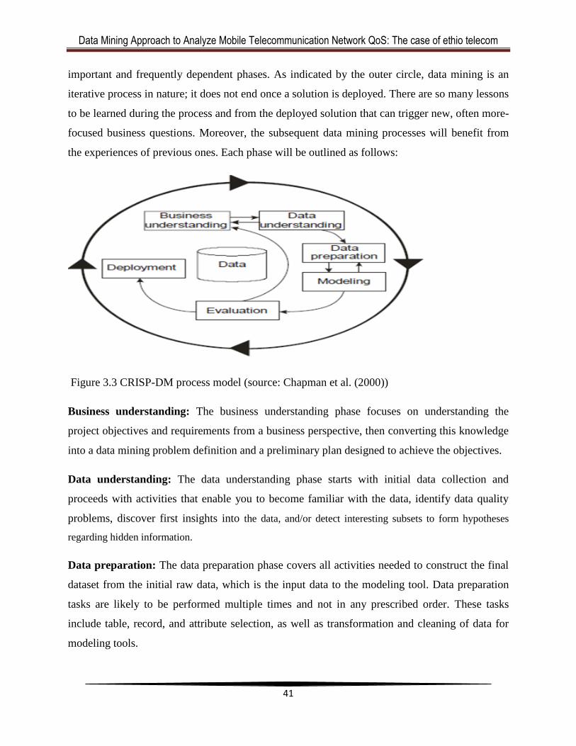
Data Mining Approach to Analyze Mobile Telecommunication Network QoS: The case of ethio telecom
41
important and frequently dependent phases. As indicated by the outer circle, data mining is an
iterative process in nature; it does not end once a solution is deployed. There are so many lessons
to be learned during the process and from the deployed solution that can trigger new, often more-
focused business questions. Moreover, the subsequent data mining processes will benefit from
the experiences of previous ones. Each phase will be outlined as follows:
Figure 3.3 CRISP-DM process model (source: Chapman et al. (2000))
Business understanding: The business understanding phase focuses on understanding the
project objectives and requirements from a business perspective, then converting this knowledge
into a data mining problem definition and a preliminary plan designed to achieve the objectives.
Data understanding: The data understanding phase starts with initial data collection and
proceeds with activities that enable you to become familiar with the data, identify data quality
problems, discover first insights into the data, and/or detect interesting subsets to form hypotheses
regarding hidden information.
Data preparation: The data preparation phase covers all activities needed to construct the final
dataset from the initial raw data, which is the input data to the modeling tool. Data preparation
tasks are likely to be performed multiple times and not in any prescribed order. These tasks
include table, record, and attribute selection, as well as transformation and cleaning of data for
modeling tools.
Data Mining Approach to Analyze Mobile Telecommunication Network QoS: The case of ethio telecom
42
Modeling: In this phase, various modeling techniques are selected and applied, and their
parameters are calibrated to optimal values. Typically, there are several techniques for the same
data mining problem type. Some techniques have specific requirements on the form of data.
Therefore, going back to the data preparation phase is often necessary.
Evaluation: At this stage in the project, you have built a model (or models) that appear to have
high quality from a data analysis perspective. Before proceeding to final deployment of the
model, it is important to thoroughly evaluate it and review the steps executed to create it, to be
certain the model properly achieves the business objectives. A key objective is to determine if
there is some important business issue that has not been sufficiently considered. At the end of
this phase, a decision on the use of the data mining results should be reached.
Deployment: Creation of the model is generally not the end of the project. Even if the purpose
of the model is to increase knowledge of the data, the knowledge gained will need to be
organized and presented in a way that the customer can use it. It often involves applying ―live‖
models within an organization‘s decision making processes
3.5 Application of Data Mining in Telecommunications
The telecommunications industry has been one of the earliest adopters of data mining technology
and will continue to accelerate this adoption as companies strive to operate more efficiently and
gain a competitive advantage in dealing with the huge amount of data generated in this area.
According to Nadaf & Kadam (2013), these data include call detail data which describes the calls
that traverse the telecommunications networks, network data which describes the state of the
hardware and software components in the network, and customer data which describes the
telecommunication customers. The amount of these data is so great that manual analysis of the
data is difficult, if not impossible.
Telecommunications data have several interesting issues for data mining. The first is concerning
scale since telecommunications databases contain billions of records and are amongst the largest
in the world. The second issue is that the raw data is often not suitable for data mining. For
example, both call detail and network data are time-series data that represent individual events.
Before this data can be effectively mined, useful ―summary‖ features must be identified and then
the data must be summarized using these features. Because many data mining applications in the
Data Mining Approach to Analyze Mobile Telecommunication Network QoS: The case of ethio telecom
43
telecommunications industry involve predicting very rare events, such as the failure of a network
element or an instance of telephone fraud, rarity is another issue that must be dealt with. The
fourth and final data mining issue concerns real-time performance; many data mining
applications, such as fraud detection, require that any learned model/rules be applied in real-time,
Nadaf & Kadam (2013); Joseph (2013).
3.5.1 Types of Telecommunication Data
Useful applications cannot be developed without understanding the various data used in
telecommunications industries. So the early step in the data mining process is to understand the
data. According to Joseph (2013), the different kinds of data used in this industry are mainly
grouped into 3 different types: Call detail data, Network data, and Customer data.
Call detail data: This is the information about the call made by the subscriber, stored as the call
detail record. As frequent calls are made by a large number of subscribers, the number of call
detail records generated is huge. Since every call is placed on the network, the details are stored.
Call detail record includes information like originating and terminating phone numbers, date,
time and duration of call. Usually these call detail records are not directly used for Data Mining.
A list of features can be generated from the call detail data such as:
Average call duration
Average number of call originated per day
Average number of call received per day
Percentage of no-answer calls
Percentage of day time calls (office hours)
Percentage of weekday calls (Monday – Friday)
These features can be used to generate a customer profile, which would be used to distinguish
residential and business customers.
Network data: Telecommunications contain thousands of interconnected network components,
that are capable of generating error and status messages which leads to a large volume of
network data. These network data are used for network management functions like fault
detection. As discussed in Weiss (2009), expert systems have been developed to analyze these
Data Mining Approach to Analyze Mobile Telecommunication Network QoS: The case of ethio telecom
44
messages automatically, since the huge volume of network messages generated cannot be
handled by technicians. However, these expert systems were expensive to develop as it is both
time-consuming and difficult to encode the relevant knowledge from the human expert. Hence
data mining technologies are used in identification of network faults by automatically extracting
knowledge from network data. Network data is also generated in real time which can be
accomplished by applying a time window to the data.
Customer data: Like any other business, telecommunication companies also have millions of
customers. Hence it is very much essential to have a database for storing the information about
these customers. Information about the customer will include:
Name of the customer
Address details
Payment history
Service plan and so on
3.5.2 Data Mining Tasks in Telecommunications
The telecommunications industry share many similarities with the retail industry in many data
mining tasks such as constructing large-scale data warehouses, performing multi-dimensional
visualization, OLAP, and in-depth analysis of trends, customer patterns, and sequential patterns.
Both industries are benefited from data mining in many aspects like business improvements, cost
reduction, customer retention, fraud analysis, and sharpening the edges of competition. Data
mining tools that are customized to be applied for the telecommunications business are
anticipated to provide solutions for the wide range of problems in this industry Han et. al. (2011).
In recent years, telecommunications have taken full advantage of access to data mining
technology. There is a fierce competition in this area, especially among telecom operators, to
improve the service quality and attract customers. In this regard, they should manage their
customers and the market itself by finding a solution to the problems of identifying customer
profile, to create and maintain their loyalty, and strategies for selling new products or services
through the application of data mining. Among the problems that can be solved by data mining
techniques in this area are: Fraud prediction in mobile telephony, Identifying loyal/profitable
customer profile, Identifying factors influencing customer behavior concerning the type of phone
Data Mining Approach to Analyze Mobile Telecommunication Network QoS: The case of ethio telecom
45
calls, Identifying risks regarding new investments in cutting-edge technologies (e.g., optic fiber,
nano-technologies, semiconductors, etc.), Identifying differences in products and services
between competitors are the vital once, Gorunescu F. (2011). Unlike the wide range of the
issues, the advent of data mining technology promised solutions to these problems. Some of
them are described in the following paragraphs.,
3.5.2.1 Fraud Detection
As indicated in Nadaf and Kadam (2013), fraud is a serious problem for telecommunications
companies that results in a loss of revenue in billions of dollars each year. There are two types of
fraud, namely subscription fraud and superimposition fraud. Subscription fraud occurs when a
customer subscribes for a service with the intention of never paying for the usage charges.
Superimposition fraud is committed by a legitimate subscription with some legitimate activity,
but also includes some ―superimposed‖ illegitimate activity by an individual other than the
account holder. In the current telecom business activity, superimposition fraud is a bigger
problem for the telecommunications industry.
3.5.2.2 Customer Segmentation and Profiling
Customer Segmentation is the process of dividing customers into the homogeneous groups
according to their common attributes. These attributes include their likes, habits, actions. And
Customer profiling means to describe the customers by their characteristics like age, gender,
economic conditions, income, culture … etc. This Customer segmentation and profiling helps the
telecommunications companies to decide which marketing actions should be taken for respective
segment and allocating the resources, Weiss (2009).
3.5.2.3 Network Fault Isolation
Telecommunications networks are extremely complex configurations of hardware, software, and
various network elements. Most of the network elements are capable of at least limited self-
diagnosis, and these elements may collectively generate millions of status and alarm messages at
each instance. In order to effectively manage the network, the status and alarm messages must be
analyzed automatically in order to identify network faults in a timely manner—or before they
occur and degrade network performance. A proactive response is essential to maintaining the
reliability of the network. Because of the volume of the data, and because a single fault may
Data Mining Approach to Analyze Mobile Telecommunication Network QoS: The case of ethio telecom
46
cause many different, seemingly unrelated, alarms to be generated, the task of network fault
isolation is quite difficult. Data mining has a role to play in generating rules for identifying
faults, Weiss (2009).
3.5.3 Local Researches in the Telecom Industry
As described in the previous paragraphs of section 3.5.2, the three main research areas of data
mining in the context of telecommunications business are Fraud detection, Customer
Segmentation and Profiling, and Network Fault Isolation. The local researches conducted on the
application of data mining for the telecommunications industry can be summarized in two
classes based on the three areas, one on the telecom fraud related to fraud detection and the other
on customer relationship management (CRM) related to Customer Segmentation and Profiling.
Melaku (2009) have conducted a research on ‗Applicability of Data Mining Techniques to
Customer Relationship Management (CRM): The Case of Ethiopian Telecommunication
Corporation's (ETC) Code Division Multiple Access (CDMA) Telephone Service.‘ On this
research, CDMA call detail record (CDR) data along with billing information and the customers
profile are collected. Different clustering and classification techniques of data mining are applied
to cluster and classify high and low value customers.
Yeshinegus (2013) have conducted a research on ‗Predictive Modeling for Fraud Detection in
Telecommunications: The Case of ethio telecom.‘ On this study an effort has been made to
predict fraudulent calls made using SIM boxes to terminate international calls. Sample Call
Detail Record (CDR) data is used along with SMS, GPRS and on line charging service (OCS)
data as a data set. Different classification methods such as J48, PART and multilayer perception
algorithms are applied to predict fraudulent calls.
According to Weiss (2009), numerous data mining applications have been deployed in the
telecommunications industry. However, most applications fall into one of the following three
categories: marketing, fraud detection, and network fault isolation and prediction. It is clearly
shown that the theme of this paper winds up on the last application.
Data Mining Approach to Analyze Mobile Telecommunication Network QoS: The case of ethio telecom
47
3.6 Review of Related works
Different studies have been made on the QoS for mobile telecommunication by different scholars
around the world. However, as to the reach of the knowledge of this researcher no local
researches have been conducted on this area.
Pitas et. al. (2011) presents a paper entitled ―QoS Mining Methods for Performance Estimation
of Mobile Radio Networks‖ on the 10th International Conference on Measurement of Speech,
Audio and Video Quality in Networks. This study present data mining methods for speech and
video quality analysis and prediction. Accordingly, it is proved that quality of speech and video
telephony services can be discovered applying algorithms like the k nearest-neighbor (KNN)
classifier, decision trees and artificial neural networks. The study concludes that learning from
QoS measurements is suitable for building evaluation and prediction models. Finally, it
recommends conducting a study on the applicability of clustering algorithms.
Fong (2011), on his study entitled ―Data Mining for Resource Planning and QoS Supports in
GSM Networks‖, uses data mining to derive rules and extract traffic patterns that reveal critical
information for setting values. The study tries to propose a new resource planning scheme that
can dynamically adjusts the resource allocations according to the latest information of the traffic
statues. As a result, resource management system is proposed for resource planning in order to
facilitate dynamic resource allocation.
Lehtim aki (2008) studies on his doctoral research named ―Data Analysis Methods for Cellular
network Performance Optimization‖, the application of various data-analysis methods for the
processing of the available measurement information in order to provide more efficient methods
for performance optimization. On this research expert-based methods have been presented for
the monitoring and analysis of multivariate cellular network performance data. These methods
allow the analysis of performance bottlenecks having an effect in multiple performance
indicators.
Multanen et. al. (2006) conduct a research entitled ―Hierarchical analysis of GSM network
performance data‖ to study a method for hierarchical examination and visualization of GSM data
using the Self-Organizing Map (SOM) both in clustering and in visualization. As a result it is
possible to reduce the amount of data and to give an extensive picture of the performance data.
Data Mining Approach to Analyze Mobile Telecommunication Network QoS: The case of ethio telecom
48
Vehviläinen (2004) have conducted a doctoral research named 'Data Mining for Managing
Intrinsic Quality of Service in Digital Mobile Telecommunications Networks'. In this study three
data mining methods; rough sets, Classification And Regression Trees (CART), and Self-
Organizing Map (SOM) were applied to the actual GSM network performance measurements
preparing a data set of 3069 instances. The results show that the analyst can make good use of
rough sets and Classification And Regression Trees (CART), because their information can be
expressed in plain language rules that preserve the variable names of the original measurement.
The study also recommends to concentrates on the preprocessing of the data set.
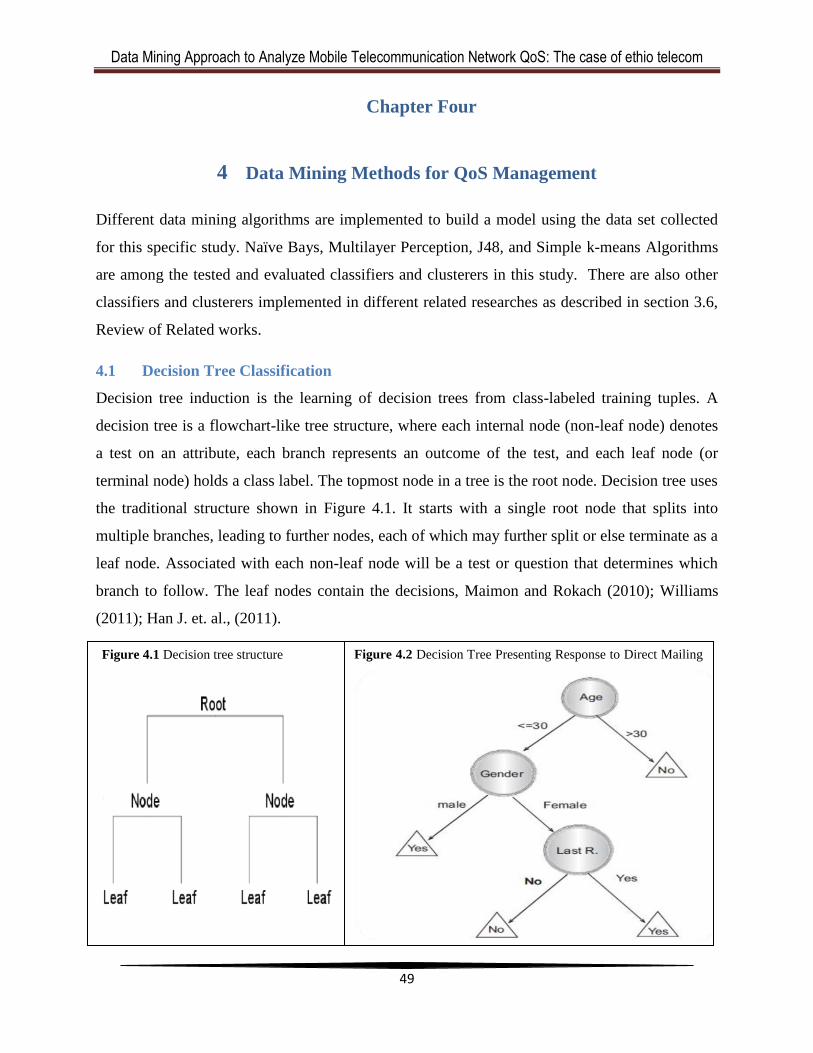
Data Mining Approach to Analyze Mobile Telecommunication Network QoS: The case of ethio telecom
49
Chapter Four
4 Data Mining Methods for QoS Management
Different data mining algorithms are implemented to build a model using the data set collected
for this specific study. Naïve Bays, Multilayer Perception, J48, and Simple k-means Algorithms
are among the tested and evaluated classifiers and clusterers in this study. There are also other
classifiers and clusterers implemented in different related researches as described in section 3.6,
Review of Related works.
4.1 Decision Tree Classification
Decision tree induction is the learning of decision trees from class-labeled training tuples. A
decision tree is a flowchart-like tree structure, where each internal node (non-leaf node) denotes
a test on an attribute, each branch represents an outcome of the test, and each leaf node (or
terminal node) holds a class label. The topmost node in a tree is the root node. Decision tree uses
the traditional structure shown in Figure 4.1. It starts with a single root node that splits into
multiple branches, leading to further nodes, each of which may further split or else terminate as a
leaf node. Associated with each non-leaf node will be a test or question that determines which
branch to follow. The leaf nodes contain the decisions, Maimon and Rokach (2010); Williams
(2011); Han J. et. al., (2011).
Figure 4.2 Decision Tree Presenting Response to Direct Mailing Figure 4.1 Decision tree structure

Data Mining Approach to Analyze Mobile Telecommunication Network QoS: The case of ethio telecom
50
Decision trees attempt to find a strong relationship between input values and target values in a
group of observations that form a data set. When a set of input values is identified as having a
strong relationship to a target value, then all of these values are grouped in a bin that becomes a
branch on the decision tree. These groupings are determined by the observed form of the
relationship between the bin values and the target, Ville (2006).
The construction of decision tree classifiers does not require any domain knowledge or
parameter setting, and therefore is appropriate for exploratory knowledge discovery. Decision
trees can handle multidimensional data. Their representation of acquired knowledge in tree form
is intuitive and generally easy to assimilate by humans. The learning and classification steps of
decision tree induction are simple and fast. Their attraction lies in the simplicity of the resulting
model, where a decision tree (at least one that is not too large) is quite easy to view, understand,
and, importantly explain. In general, decision tree classifiers have good accuracy. However
decision trees do not always deliver the best performance, and represent a trade-off between
performance and simplicity of explanation and successful use may depend on the data at hand,
Williams (2011); Han J. et. al. (2011).
According to Gorunescu (2011), decision trees have three classical approaches:
i. Classification trees: when the prediction result is the class membership of data;
ii. Regression trees: when the predicted result is considered as a real number (e.g., oil price,
value of a house, stock price, etc.);
iii. CART (or C&RT), i.e., Classification And Regression Tree: when both Classification
and Regression trees are considered.
A. Tree Size
Generally, decision makers prefer less complex decision trees, since it is considered more
comprehensive and easy to understand. According to Breiman et al. (1984), the tree complexity
has a crucial effect on its accuracy. The tree complexity is explicitly controlled by the stopping
criteria used and the pruning method employed. Usually the tree complexity is measured by one
of the following metrics: the total number of nodes, total number of leaves, tree depth and
number of attributes used.

Data Mining Approach to Analyze Mobile Telecommunication Network QoS: The case of ethio telecom
51
B. Rule Induction in Trees
As described in Han J. et. al. (2011), there is a close relationship between decision tree induction
and rule induction. Each path from the root of a decision tree to one of its leaves can be
transformed into a rule simply by conjoining the tests along with the path to form the antecedent
part, and taking the leaf‘s class prediction as the class value. For example, one of the paths in
Figure 4.2 can be transformed into the rule: If customer age is less than or equal to 30, and the
gender of the customer is ―Male‖ – then the customer will respond to the mail. The resulting rule
set can then be simplified to improve its comprehensibility to a human user, and possibly its
accuracy.
C. Splitting Criteria
As indicated in Maimon and Rokach (2010), there are two types of splitting criteria in decision
tree: Univariate Splitting Criteria and Multivariate Splitting Criteria.
Univariate Splitting Criteria: Univariate means that an internal node is split according to the
value of a single attribute. Consequently the inducer searches for the best attribute upon which to
split. The most common criteria in the literature includes: Impurity-based Criteria, Information
Gain, Gini Index, Gain Ratio, etc.
Multivariate Splitting Criteria: In multivariate splitting criteria, several attributes may
participate in a single node split test. Obviously, finding the best multivariate criteria is more
complicated than finding the best univariate split. Furthermore, although this type of criteria may
dramatically improve the tree‘s performance, these criteria are much less popular than the
univariate criteria. Most of the multivariate splitting criteria is based on the linear combination of
the input attributes.
D. Stopping Criteria
The growing phase continues until a stopping criterion is triggered. Conditions that are common
for stopping rules are: All instances in the training set belong to a single value of y; The
maximum tree depth has been reached; The number of cases in the terminal node is less than the
minimum number of cases for parent nodes; If the node were split, the number of cases in one or
more child nodes would be less than the minimum number of cases for child nodes; The best
Data Mining Approach to Analyze Mobile Telecommunication Network QoS: The case of ethio telecom
52
splitting criterion is not greater than a certain threshold, Han J. et. al. (2011); Maimon and
Rokach (2010).
E. Pruning
Employing tightly stopping criteria tends to create small and under–fitted decision trees. On the
other hand, using loosely stopping criteria tends to generate large decision trees that are over–
fitted to the training set. Pruning methods originally suggested in Breiman et al., (1984) were
developed for solving this dilemma. According to this methodology, a loosely stopping criterion
is used, letting the decision tree to over-fit the training set. Then the over-fitted tree is cut back
into a smaller tree by removing sub–branches that are not contributing to the generalization
accuracy. It has been shown in various studies that employing pruning methods can improve the
generalization performance of a decision tree, especially in noisy domains.
When the goal is to produce a sufficiently accurate compact concept description, pruning is
highly useful. Within this process, the initial decision tree is seen as a completely accurate one.
Thus the accuracy of a pruned decision tree indicates how close it is to the initial tree, Maimon
and Rokach (2010).
The dramatic growth of information system enable huge amount of data to be generated and
collected day to day in many application areas so that there is a need for data mining algorithms
such as decision tree to deal with this large datasets. I58, SLIQ, SPRINT, C4.5 (JAVA
implementation is J48), CART and CHAID are among the decision tree algorithms that are
described in many literatures. This study will concentrate on J48 decision tree algorithm which is
the JAVA implementation of C4.5 algorithm, as it is used for experimentation.
4.1.1 J48 Decision Tree Algorithm
The best known decision tree learner is C4.5 by Quinlan (1993) and its java version, J48 the
more recent upgrade by the same author, which is widely used and has been incorporated into
commercial data mining tools as well as in the publicly available WEKA Data Mining toolbox. It
is reliable, efficient and capable of dealing with large sets of training examples, Maimon and
Rokach (2010).

Data Mining Approach to Analyze Mobile Telecommunication Network QoS: The case of ethio telecom
53
It generates a classification-decision tree for the given data-set by recursive partitioning of data.
The decision is grown using Depth-first strategy. The algorithm considers all the possible tests
that can split the data set and selects a test that gives the best information gain. For each discrete
attribute, one test with outcomes as many as the number of distinct values of the attribute is
considered. For each continuous attribute, binary tests involving every distinct values of the
attribute are considered. In order to gather the entropy gain of all these binary tests efficiently,
the training data set belonging to the node in consideration is sorted for the values of the
continuous attribute and the entropy gains of the binary cut based on each distinct values are
calculated in one scan of the sorted data. This process is repeated for each continuous attributes,
Zhao and Zhang (2007).
As described in Wu et al., (2007), given a set S of cases, C4.5 first grows an initial tree using the
divide-and-conquer algorithm as follows:
• If all the cases in S belong to the same class or S is small, the tree is a leaf labeled with
the most frequent class in S.
• Otherwise, choose a test based on a single attribute with two or more outcomes. Make the
test the root of the tree with one branch for each outcome of the test, partition S into
corresponding subsets S1, S2, . . . according to the outcome for each case, and apply the
same procedure recursively to each subset.
There are usually many tests that could be chosen in this last step. C4.5 uses two heuristic
criteria to rank possible tests: information gain, which minimizes the total entropy of the subsets
{Si } (but is heavily biased towards tests with numerous outcomes), and the default gain ratio
that divides information gain by the information provided by the test outcomes. Attributes can be
either numeric or nominal and this determines the format of the test outcomes. For a numeric
attribute A they are {A ≤ h, A > h} where the threshold h is found by sorting S on the values of
A and choosing the split between successive values that maximize the criterion above. An
attribute A with discrete values has by default one outcome for each value, but an option allows
the values to be grouped into two or more subsets with one outcome for each subset. The initial
tree is then pruned to avoid over-fitting, Wu et al., (2007).

Data Mining Approach to Analyze Mobile Telecommunication Network QoS: The case of ethio telecom
54
4.2 Naïve Bayes Classification
Bayesian classifiers are statistical classifiers. They can predict class membership probabilities
such as the probability that a given tuple belongs to a particular class. Bayesian classification is
based on Bayes‘ theorem. Studies comparing classification algorithms have found a simple
Bayesian classifier known as the naïve Bayesian classifier to be comparable in performance with
decision tree and selected neural network classifiers. Bayesian classifiers have also exhibited
high accuracy and speed when applied to large databases. The naive Bayes classifier assumes
that attributes are independent, but it is still surprisingly powerful for many applications Zaki and
Meira (2013); Han J. et. al. (2011).
As indicated in Harrington (2012), the advantage of Naïve Bayes classification is that it works
with a small amount of data and handles multiple classes. However it is sensitive to how the
input data is prepared. In general, Naïve Bayes works with nominal values.
4.2.1 Bays Theorem
According to Harrington (2012), Bayesian probability is named after Thomas Bayes, who was an
eighteenth-century theologian. Bayesian probability allows prior knowledge and logic to be
applied to uncertain statements.
As indicated in Zaki and Meira (2013), let the training dataset D consist of n points of xi in a d-
dimensional space, and let yi denote the class for each point, with yi ∈ {c1, c2… ck}. The Bayes
classifier directly uses the Bayes theorem to predict the class for a new test instance, x. It
estimates the posterior probability P(ci|x) for each class ci, and chooses the class that has the
largest probability. The Bayes theorem allows inverting the posterior probability in terms of the
likelihood and prior probability, which can be written as:
Where P(x|ci) is the likelihood, defined as the probability of observing x assuming that the true
class is ci, P(ci) is the prior probability of class ci, and P(x) is the probability of observing x from
any of the k classes, given as

Data Mining Approach to Analyze Mobile Telecommunication Network QoS: The case of ethio telecom
55
Cios K., Pedrycz W., Swiniarski R., Kurgan L. (2007) stated Bayes‘ classification rule for
multiclass objects with a multidimensional feature vector as:
―Given an object with a corresponding feature vector value x, assign an object to a class cj with
the highest a posteriori conditional probability P (cj/x).‖
In other words:
―For a given object with a given value x of a feature vector, assign an object to class cj when
P (cj/x) > P (ci/x), i = 1, 2…, l; i ≠ j‖
The conditional probability p (ci/x) is difficult to ascertain; however, using Bayes‘ theorem, we
express it in terms of p (x/ci), P (ci) and P (x):
―A given object, with a given value x of a feature vector, can be classified as belonging to class
cj when
After canceling the scaling probability p(x) from both sides, we obtain the following form of the
Bayes classification rule:
―Assign an object with a given value x of a feature vector to class cj when
p (x/cj) P (cj) > p (x/ci) P (ci) , i = 1, 2,…,l; i ≠ j‖
In the sense of the minimization of the probability of classification, Bayes‘ error rule is the
theoretically optimal classification rule. In other words, there is no other classification rule that
yields lower values of the classification error.
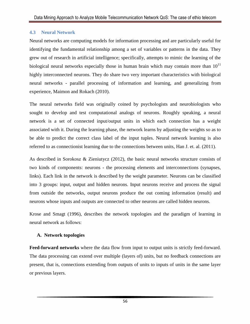
Data Mining Approach to Analyze Mobile Telecommunication Network QoS: The case of ethio telecom
56
4.3 Neural Network
Neural networks are computing models for information processing and are particularly useful for
identifying the fundamental relationship among a set of variables or patterns in the data. They
grew out of research in artificial intelligence; specifically, attempts to mimic the learning of the
biological neural networks especially those in human brain which may contain more than 1011
highly interconnected neurons. They do share two very important characteristics with biological
neural networks - parallel processing of information and learning, and generalizing from
experience, Maimon and Rokach (2010).
The neural networks field was originally coined by psychologists and neurobiologists who
sought to develop and test computational analogs of neurons. Roughly speaking, a neural
network is a set of connected input/output units in which each connection has a weight
associated with it. During the learning phase, the network learns by adjusting the weights so as to
be able to predict the correct class label of the input tuples. Neural network learning is also
referred to as connectionist learning due to the connections between units, Han J. et. al. (2011).
As described in Sorokosz & Zieniutycz (2012), the basic neural networks structure consists of
two kinds of components: neurons - the processing elements and interconnections (synapses,
links). Each link in the network is described by the weight parameter. Neurons can be classified
into 3 groups: input, output and hidden neurons. Input neurons receive and process the signal
from outside the networks, output neurons produce the out coming information (result) and
neurons whose inputs and outputs are connected to other neurons are called hidden neurons.
Krose and Smagt (1996), describes the network topologies and the paradigm of learning in
neural network as follows:
A. Network topologies
Feed-forward networks where the data flow from input to output units is strictly feed-forward.
The data processing can extend over multiple (layers of) units, but no feedback connections are
present, that is, connections extending from outputs of units to inputs of units in the same layer
or previous layers.

Data Mining Approach to Analyze Mobile Telecommunication Network QoS: The case of ethio telecom
57
Recurrent networks that do contain feedback connections; contrary to feed-forward networks,
the dynamical properties of the network are important. In some cases, the activation values of the
units undergo a relaxation process such that the network will evolve to a stable state in which
these activations do not change anymore. In other applications, the change of the activation
values of the output neurons is significant, such that the dynamical behavior constitutes the
output of the network.
Classical examples of feed-forward networks include the Perceptron and Adaline; and that of
recurrent networks are the Hopfield network, the Elman network (where some of the hidden unit
activation values are fed back to an extra set of input units), and the Jordan network (where
output values are fed back into hidden units).
B. Paradigms of learning
We can categories the learning situations in two distinct sorts. These are:
Supervised learning or Associative learning in which the network is trained by providing it
with input and matching output patterns. These input-output pairs can be provided by an external
teacher, or by the system which contains the network (self-supervised).
Unsupervised learning or Self-organization in which an output unit is trained to respond to
clusters of pattern within the input. In this paradigm the system is supposed to discover
statistically salient features of the input population. Unlike the supervised learning paradigm,
there is no a priori set of categories into which the patterns are to be classified; rather the system
must develop its own representation of the input stimuli.
4.3.1 Multilayer perception
Multilayer perceptions (MLPs) are the best known and most widely used kind of neural network.
They are formed by units of the type shown in Figure 4.3. Each of these units forms a weighted
sum of its inputs, to which a constant term is added. This sum is then passed through a
nonlinearity, which is often called its activation function. Most often, units are interconnected in
a feed-forward manner, that is, with interconnections that do not form any loops, as shown in
Figure 4.4. For some kinds of applications, recurrent (i.e. non-feed-forward) networks in which
some of the interconnections form loops are also used, Krose and Smagt (1996).
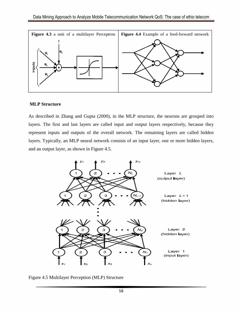
Data Mining Approach to Analyze Mobile Telecommunication Network QoS: The case of ethio telecom
58
MLP Structure
As described in Zhang and Gupta (2000), in the MLP structure, the neurons are grouped into
layers. The first and last layers are called input and output layers respectively, because they
represent inputs and outputs of the overall network. The remaining layers are called hidden
layers. Typically, an MLP neural network consists of an input layer, one or more hidden layers,
and an output layer, as shown in Figure 4.5.
Figure 4.5 Multilayer Perception (MLP) Structure
Figure 4.3 a unit of a multilayer Perceptron
Figure 4.4 Example of a feed-forward network

Data Mining Approach to Analyze Mobile Telecommunication Network QoS: The case of ethio telecom
59
Suppose the total number of layers is L. The 1st layer is the input layer, the L
th layer is the output
layer, and layers 2 to L-1 are hidden layers. Let the number of neurons in lth
layer be Nl, l = 1,
2… L.
Let Wlij represent the weight of the link between j
th neuron of l-1th layer and i
th neuron of lth
layer,, 1<=j<=Nl-1, 1<=I<=Nl. Let xi represent the ith
external input to the MLP, and zi be the
output of ith
neuron of lth
layer. We introduce an extra weight parameter for each neuron, wli0,
representing the bias for ith
neuron of lth
layer. As such, w of MLP includes wlij, j = 0, 1…Nl-1,
i= l=2, 3… L, that is,
As briefly described in Han J. et. al. (2011); Maimon and Rokach (2010), the advantage of neural
networks include: they involve long training times, high tolerance of noisy data as well as ability
to classify patterns on which they have not been trained. They can be used when there is a little
knowledge regarding the relationships between attributes and classes. They are well suited for
continuous-valued inputs and outputs, unlike most decision tree algorithms. They have been
successful on a wide array of real-world data, including handwritten character recognition,
pathology and laboratory medicine, and training a computer to pronounce English text. Neural
network algorithms are inherently parallel; parallelization techniques can be used to speed up the
computation process. In addition, several techniques have been recently developed for rule
extraction from trained neural networks. These factors contribute to the usefulness of neural
networks for classification and numeric prediction in data mining. However neural networks
have been criticized for their poor interpretability. For example, it is difficult for humans to
interpret the symbolic meaning behind the learned weights and of ―hidden units‖ in the network.
These features initially made neural networks less desirable for data mining.
4.4 k-Means Clustering
As described in Harrington P. (2012), k-means is an algorithm that will find k clusters for a
given dataset. The number of clusters k is user defined. Each cluster is described by a single
point known as the centroid. Centroid means the single point is at the center of all the points in
the cluster.

Data Mining Approach to Analyze Mobile Telecommunication Network QoS: The case of ethio telecom
60
As indicated in Han J. et. al. (2011), this centroid can be defined by the mean or medoid of the
objects (or points) assigned to the cluster. The difference between an object p ∈ Ci and ci, the
representative of the cluster, is measured by dist (p, ci), where dist (x, y) is the Euclidean
distance between two points x and y. The quality of cluster Ci can be measured by the within-
cluster variation, which is the sum of squared error between all objects in Ci and the centroid ci,
defined as:
∑ ∑
∈ Dist (p, ci) 2
Where E is the sum of the squared error for all objects in the data set; p is the point in space
representing a given object; and ci is the centroid of cluster Ci (both p and ci are
multidimensional). In other words, for each object in each cluster, the distance from the object to
its cluster center is squared, and the distances are summed. This objective function tries to make
the resulting k clusters as compact and as separate as possible.
4.4.1 k-Means Algorithm
Gorunescu (2011) describes the general scheme of the k-means algorithm as follows:
1) Select k points at random as cluster centers.
2) Assign instances to their closest cluster center according to some similarity
distance function.
3) Calculate the centroid or mean of all instances in each cluster (this is the ‘mean‘
part of the algorithm).
4) Cluster the data into k groups where k is predefined.
5) GOTO the step 3. Continue until the same points are assigned to each cluster in
consecutive rounds.
The time complexity of the k-means algorithm is O (n*k*t), where n is the total number of
objects, k is the number of clusters, and t is the number of iterations. Normally, k ≪ n and t ≪ n,
therefore, the method is relatively scalable and efficient in processing large data sets, Han J. et.
al. (2011).
Data Mining Approach to Analyze Mobile Telecommunication Network QoS: The case of ethio telecom
61
According to Maimon and Rokach (2010), the k-means algorithm has an advantage when it is
compared to other clustering methods (e.g. hierarchical clustering methods) on that it has non-
linear complexity, ease of interpretation, simplicity of implementation, speed of convergence and
adaptability to sparse data. However the k-means algorithm works well only on data sets having
isotropic clusters, and is not as versatile as single link algorithms. Moreover, this algorithm is
sensitive to noisy data and outliers (a single outlier can increase the squared error dramatically);
it is applicable only when mean is defined (namely, for numeric attributes); and it requires the
number of clusters in advance, which is not trivial when no prior knowledge is available. The use
of the k-means algorithm is often limited to numeric attributes.
Han J. et. al. (2011) points out approaches to make the k-means method more efficient on large
data sets. One is to use a good-sized set of samples in clustering. Another is to employ a filtering
approach that uses a spatial hierarchical data index to save costs when computing means. A third
approach explores the micro-clustering idea, which first groups nearby objects into ―micro-
clusters‖ and then performs k-means clustering on the micro-clusters.
Data Mining Approach to Analyze Mobile Telecommunication Network QoS: The case of ethio telecom
62
Chapter Five
5 Experimentation and Analysis
As indicated from the outset, the objective of this research is to analyze the performance of the
GSM network based on the data extracted from the ethio telecom live mobile network using data
mining techniques. Thus, the experimentation is conducted on the basis of the selected process
model which is Knowledge Data Discovery (KDD) indicated in Section 1.6. Different data
mining algorithms such as J48 Decision Tree, Naïve Bayes, Multilayer Perception, and k-means
are applied in this experimentation. On the top of all these, Knowledge from domain experts is
crucial to understand the application domain where this study is conducted.
5.1 Experiment Design
The computer used for this experimentation is Dell-E5430, Intel (R), Core I7, CPU 3.oo GHz,
RAM 4.00 GHz, and 32 bit operating system. Different software tools are involved in this
experiment including Microsoft Excel to filter out and format the desired data before it is
changed into Attribute Relation File Format (ARFF) data format. The open source data mining
tool selected for this study is Weka since it is platform independent as it is written in java and
also based on the researcher‘s familiarity with the tool. The Weka version used for this specific
experimentation is Weka 3.7.11.
5.2 KDD Processes
As described in section 3.4.1, the KDD process model described from the practical viewpoint
proposed by Fayyad et al. (1996b) can be performed with in nine steps: Learning the application
domain, creating a target data set, data cleaning and preprocessing, data reduction and projection,
choosing the function of data mining, choosing the data mining algorithm, data mining,
interpretation, and using the discovered knowledge.
5.2.1 Learning the application domain
In order to acquire the domain knowledge on the application area of telecommunication network
environment relevant books, researches, and manuals are referred as well as practical knowledge
Data Mining Approach to Analyze Mobile Telecommunication Network QoS: The case of ethio telecom
63
of domain experts such as telecommunication engineers in the actual network optimization task
has been acquired through unstructured interview. Moreover, the researcher‘s previous
experience is also helpful to align the goal of the study with the application area.
5.2.2 Creating target data set
As indicated from the outset, the target data set used for this study will be extracted from the
network management system database of the live telecommunication mobile network for the
cells covered under the scope. Three kinds of data sets are extracted based on the time period
where the KPI measurements are taken. The first indicates a one day or 24 Hour KPI
measurement per one hour query granularity where the query time is 2013-12-30 00:00:00 -
2013-12-31 00:00:00, the second indicates the day high traffic hour (10:00 to 11:00) and the
night high traffic hour (20:00 to 21:00) per one hour query granularity where the query time is
2013-12-23 00:00:00 - 2013-12-30 00:00:00 and the effective time is 10:00:00-11:00:00
20:00:00-21:00:00 , and the third indicates a one month KPI measurement per one day query
granularity where the Query time is 2013-11-01 00:00:00 - 2013-12-01 00:00:00. The initial
data set contains more than 270 attributes and 33,331 rows for the first, 19,420 rows for the
second and 40,741 rows for the third data set.
The reason that the data sets are extracted in three kinds is for simplicity of analysis. The one day
KPI dataset enable to observe the cumulative effects of the KPI values in 24 hour, the day and
night high traffic hour KPI dataset enable to observe the effects of the KPIs during high traffic
hour, and the one month KPI dataset enables to observe the consistency and the cumulative
effects of the KPI values within one month.
5.2.3 Data cleaning and preprocessing
As indicated in the previous section the dataset extracted for this study contains more than 270
attributes (KPIs) however nineteen of these attributes are not informative for this specific study
and removed in order to clean the data. These attributes include: Index, Start Time, End Time,
Query Granularity, SUBNETWORK, SUBNETWORK Name, ME Name, ME, SITE, BTS,
SITE Name, BTS NAME, Location(LAC), CI(CI), cell latitude, cell longitude, cell anteHeight,
cell anteAzimuth, cell address.
Data Mining Approach to Analyze Mobile Telecommunication Network QoS: The case of ethio telecom
64
As described in Witten, Frank, and Hall (2011), errors that appear during measurement of
numeric values might cause outliers. Erroneous values often create a significant deviation from
the pattern that might be extracted in the remaining values. Thus, such inaccurate values should
be treated though it is difficult to find, particularly without specialist domain knowledge. Such
kinds of problems are visualized in the extracted data set of two specific KPIs, Standalone
Dedicated Control Channel (SDCCH) in service rate and Traffic Channel (TCH) in service rate,
whose value is below 50%. These KPIs generally indicate the health of the TRX in the
corresponding cell, which might directly or indirectly affected by a certain alarm event (minor,
major, or critical) generated in the interconnected network element. In this regard, it is
mandatory to refer the recommendation of experts in the mobile network optimization and to
examine the data set at hand.
When the data set is examined for these two KPIs, SDCCH in service rate and TCH in service
rate of values less than or equal to 50%, it is possible to generalize that the corresponding values
of other KPIs are subjected to inaccurate value. Even in the case of both SDCCH in service rate
and TCH in service rate equals 0% (when the cell is totally down), out of ten KPIs eight of them
have a KPI value even better than the standard for most of the instances. This can be taken as
manifestation of inaccuracy. As shown in Table 5.1 only Call Success Rate (CSR) and Call
Setup Success Rate (CSSR) KPIs respond to the very decrease of both SDCCH and TCH in
service rate, the rest KPIs (SDCCH-CR, TCH-CR, DCR, SDCCH-CD, TCH-CDR, HOSR,
HOSR-I, and HOSR-O) indicate a KPI value even better than the standard indicated in the
heading columns.
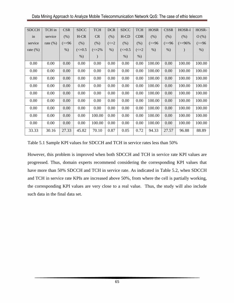
Data Mining Approach to Analyze Mobile Telecommunication Network QoS: The case of ethio telecom
65
SDCCH
in
service
rate (%)
TCH in
service
rate (%)
CSR
(%)
(>=96
%)
SDCC
H-CR
(%)
(<=0.5
%)
TCH
CR
(%)
(<=2%
)
DCR
(%)
(<=2
%)
SDCC
H-CD
(%)
(<=0.5
%)
TCH
CDR
(%)
(<=2
%)
HOSR
(%)
(>=96
%)
CSSR
(%)
(>=96
%)
HOSR-I
(%)
(>=96%
)
HOSR-
O (%)
(>=96
%)
0.00 0.00 0.00 0.00 0.00 0.00 0.00 0.00 100.00 0.00 100.00 100.00
0.00 0.00 0.00 0.00 0.00 0.00 0.00 0.00 100.00 0.00 100.00 100.00
0.00 0.00 0.00 0.00 0.00 0.00 0.00 0.00 100.00 0.00 100.00 100.00
0.00 0.00 0.00 0.00 0.00 0.00 0.00 0.00 100.00 0.00 100.00 100.00
0.00 0.00 0.00 0.00 0.00 0.00 0.00 0.00 100.00 0.00 100.00 100.00
0.00 0.00 0.00 0.00 0.00 0.00 0.00 0.00 100.00 0.00 100.00 100.00
0.00 0.00 0.00 0.00 0.00 0.00 0.00 0.00 100.00 0.00 100.00 100.00
0.00 0.00 0.00 0.00 100.00 0.00 0.00 0.00 100.00 0.00 100.00 100.00
0.00 0.00 0.00 0.00 100.00 0.00 0.00 0.00 100.00 0.00 100.00 100.00
33.33 30.16 27.33 45.82 70.10 0.87 0.05 0.72 94.33 27.57 96.88 88.89
Table 5.1 Sample KPI values for SDCCH and TCH in service rates less than 50%
However, this problem is improved when both SDCCH and TCH in service rate KPI values are
progressed. Thus, domain experts recommend considering the corresponding KPI values that
have more than 50% SDCCH and TCH in service rate. As indicated in Table 5.2, when SDCCH
and TCH in service rate KPIs are increased above 50%, from where the cell is partially working,
the corresponding KPI values are very close to a real value. Thus, the study will also include
such data in the final data set.
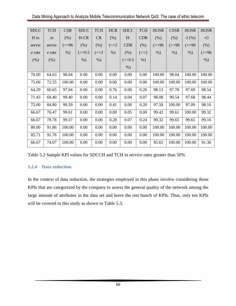
Data Mining Approach to Analyze Mobile Telecommunication Network QoS: The case of ethio telecom
66
SDCC
H in
servic
e rate
(%)
TCH
in
servic
e rate
(%)
CSR
(%)
(>=96
%)
SDCC
H-CR
(%)
(<=0.5
%)
TCH
CR
(%)
(<=2
%)
DCR
(%)
(<=2
%)
SDCC
H-
CDR
(%)
(<=0.5
%)
TCH
CDR
(%)
(<=2
%)
HOSR
(%)
(>=96
%)
CSSR
(%)
(>=96
%)
HOSR
-I (%)
(>=96
%)
HOSR
-O
(%)
(>=96
%)
70.00 64.63 98.04 0.00 0.00 0.00 0.00 0.00 100.00 98.04 100.00 100.00
75.00 72.55 100.00 0.00 0.00 0.00 0.00 0.00 100.00 100.00 100.00 100.00
64.29 60.65 97.04 0.00 0.00 0.76 0.00 0.20 98.13 97.78 97.69 98.54
71.43 69.40 99.40 0.00 0.00 0.14 0.04 0.07 98.08 99.54 97.68 98.44
75.00 84.80 99.59 0.00 0.00 0.41 0.00 0.20 97.58 100.00 97.09 98.16
66.67 76.47 99.61 0.00 0.00 0.00 0.05 0.00 99.42 99.61 100.00 99.32
66.67 78.78 99.37 0.00 0.00 0.28 0.07 0.24 99.32 99.65 99.65 99.16
80.00 91.86 100.00 0.00 0.00 0.00 0.00 0.00 100.00 100.00 100.00 100.00
85.71 91.76 100.00 0.00 0.00 0.00 0.00 0.00 100.00 100.00 100.00 100.00
66.67 74.07 100.00 0.00 0.00 0.00 0.00 0.00 95.65 100.00 100.00 91.36
Table 5.2 Sample KPI values for SDCCH and TCH in service rates greater than 50%
5.2.4 Data reduction
In the context of data reduction, the strategies employed in this phase involve considering those
KPIs that are categorized by the company to assess the general quality of the network among the
large amount of attributes in the data set and leave the rest bunch of KPIs. Thus, only ten KPIs
will be covered in this study as shown in Table 5.3.
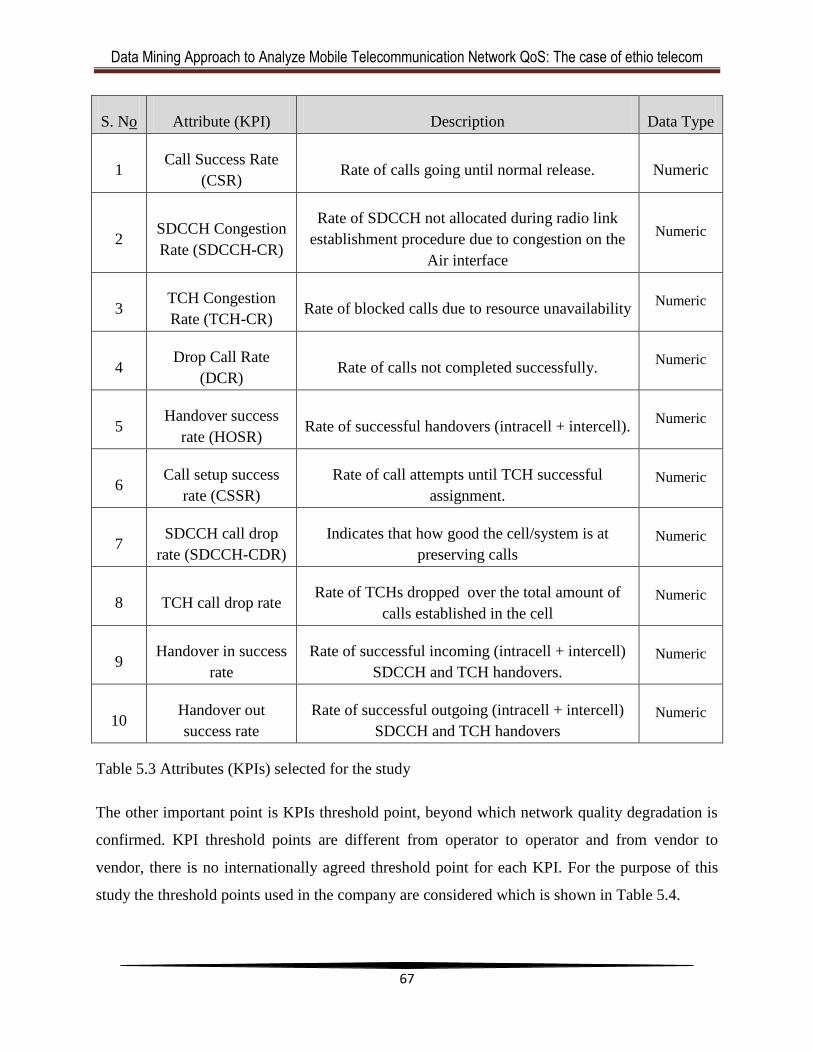
Data Mining Approach to Analyze Mobile Telecommunication Network QoS: The case of ethio telecom
67
S. No Attribute (KPI) Description Data Type
1 Call Success Rate
(CSR) Rate of calls going until normal release. Numeric
2 SDCCH Congestion
Rate (SDCCH-CR)
Rate of SDCCH not allocated during radio link
establishment procedure due to congestion on the
Air interface
Numeric
3 TCH Congestion
Rate (TCH-CR) Rate of blocked calls due to resource unavailability
Numeric
4 Drop Call Rate
(DCR) Rate of calls not completed successfully.
Numeric
5 Handover success
rate (HOSR) Rate of successful handovers (intracell + intercell).
Numeric
6 Call setup success
rate (CSSR)
Rate of call attempts until TCH successful
assignment.
Numeric
7 SDCCH call drop
rate (SDCCH-CDR)
Indicates that how good the cell/system is at
preserving calls
Numeric
8 TCH call drop rate Rate of TCHs dropped over the total amount of
calls established in the cell
Numeric
9 Handover in success
rate
Rate of successful incoming (intracell + intercell)
SDCCH and TCH handovers.
Numeric
10 Handover out
success rate
Rate of successful outgoing (intracell + intercell)
SDCCH and TCH handovers
Numeric
Table 5.3 Attributes (KPIs) selected for the study
The other important point is KPIs threshold point, beyond which network quality degradation is
confirmed. KPI threshold points are different from operator to operator and from vendor to
vendor, there is no internationally agreed threshold point for each KPI. For the purpose of this
study the threshold points used in the company are considered which is shown in Table 5.4.
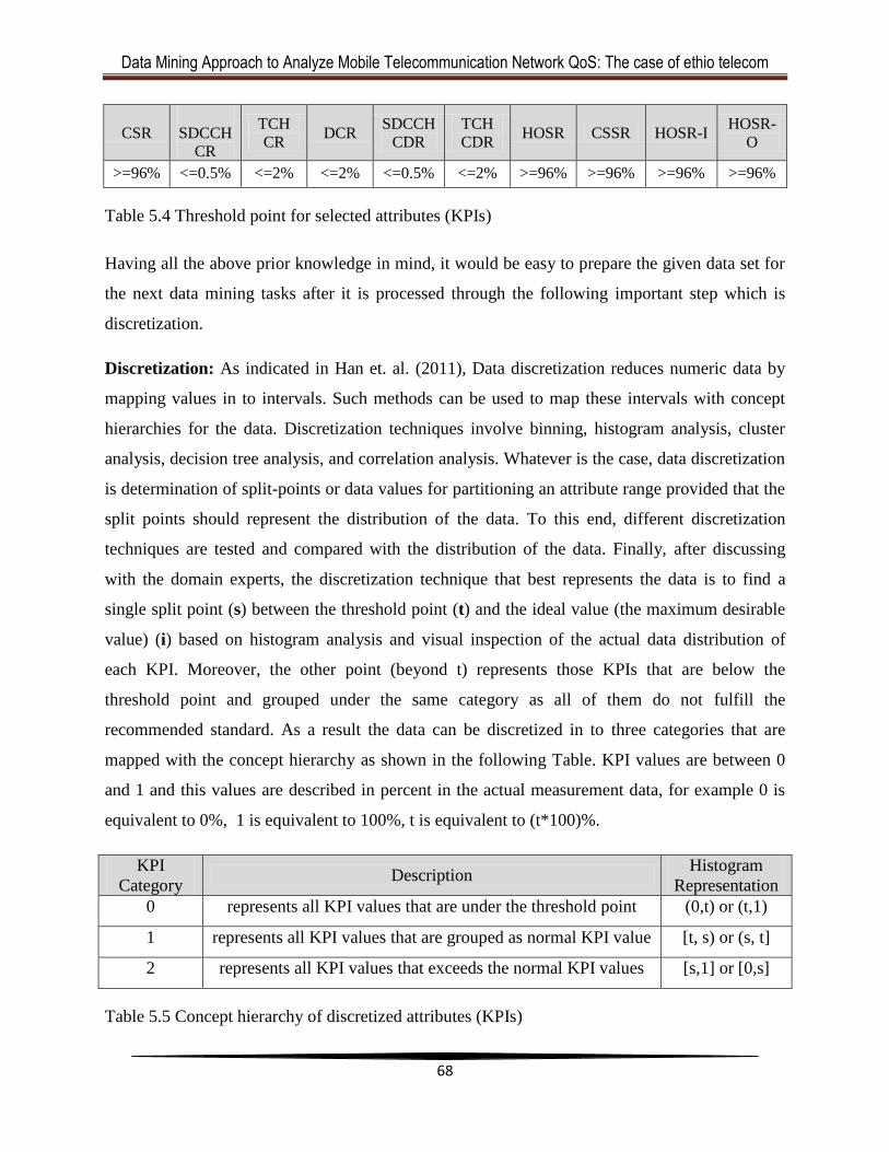
Data Mining Approach to Analyze Mobile Telecommunication Network QoS: The case of ethio telecom
68
CSR
SDCCH
CR
TCH
CR DCR
SDCCH
CDR
TCH
CDR HOSR CSSR HOSR-I
HOSR-
O
>=96% <=0.5% <=2% <=2% <=0.5% <=2% >=96% >=96% >=96% >=96%
Table 5.4 Threshold point for selected attributes (KPIs)
Having all the above prior knowledge in mind, it would be easy to prepare the given data set for
the next data mining tasks after it is processed through the following important step which is
discretization.
Discretization: As indicated in Han et. al. (2011), Data discretization reduces numeric data by
mapping values in to intervals. Such methods can be used to map these intervals with concept
hierarchies for the data. Discretization techniques involve binning, histogram analysis, cluster
analysis, decision tree analysis, and correlation analysis. Whatever is the case, data discretization
is determination of split-points or data values for partitioning an attribute range provided that the
split points should represent the distribution of the data. To this end, different discretization
techniques are tested and compared with the distribution of the data. Finally, after discussing
with the domain experts, the discretization technique that best represents the data is to find a
single split point (s) between the threshold point (t) and the ideal value (the maximum desirable
value) (i) based on histogram analysis and visual inspection of the actual data distribution of
each KPI. Moreover, the other point (beyond t) represents those KPIs that are below the
threshold point and grouped under the same category as all of them do not fulfill the
recommended standard. As a result the data can be discretized in to three categories that are
mapped with the concept hierarchy as shown in the following Table. KPI values are between 0
and 1 and this values are described in percent in the actual measurement data, for example 0 is
equivalent to 0%, 1 is equivalent to 100%, t is equivalent to (t*100)%.
KPI
Category Description
Histogram
Representation
0 represents all KPI values that are under the threshold point (0,t) or (t,1)
1 represents all KPI values that are grouped as normal KPI value [t, s) or (s, t]
2 represents all KPI values that exceeds the normal KPI values [s,1] or [0,s]
Table 5.5 Concept hierarchy of discretized attributes (KPIs)
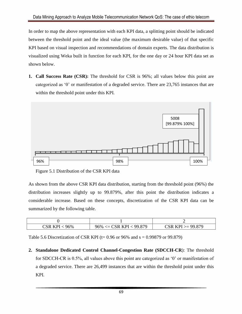
Data Mining Approach to Analyze Mobile Telecommunication Network QoS: The case of ethio telecom
69
In order to map the above representation with each KPI data, a splitting point should be indicated
between the threshold point and the ideal value (the maximum desirable value) of that specific
KPI based on visual inspection and recommendations of domain experts. The data distribution is
visualized using Weka built in function for each KPI, for the one day or 24 hour KPI data set as
shown below.
1. Call Success Rate (CSR): The threshold for CSR is 96%; all values below this point are
categorized as ‗0‘ or manifestation of a degraded service. There are 23,765 instances that are
within the threshold point under this KPI.
Figure 5.1 Distribution of the CSR KPI data
As shown from the above CSR KPI data distribution, starting from the threshold point (96%) the
distribution increases slightly up to 99.879%, after this point the distribution indicates a
considerable increase. Based on these concepts, discretization of the CSR KPI data can be
summarized by the following table.
0 1 2
CSR KPI < 96% 96% <= CSR KPI < 99.879 CSR KPI >= 99.879
Table 5.6 Discretization of CSR KPI (t= 0.96 or 96% and s = 0.99879 or 99.879)
2. Standalone Dedicated Control Channel-Congestion Rate (SDCCH-CR): The threshold
for SDCCH-CR is 0.5%, all values above this point are categorized as ‗0‘ or manifestation of
a degraded service. There are 26,499 instances that are within the threshold point under this
KPI.
5008 [99.879% 100%]
96% 98% 100%
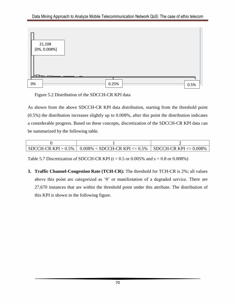
Data Mining Approach to Analyze Mobile Telecommunication Network QoS: The case of ethio telecom
70
Figure 5.2 Distribution of the SDCCH-CR KPI data
As shown from the above SDCCH-CR KPI data distribution, starting from the threshold point
(0.5%) the distribution increases slightly up to 0.008%, after this point the distribution indicates
a considerable progress. Based on these concepts, discretization of the SDCCH-CR KPI data can
be summarized by the following table.
0 1 2
SDCCH-CR KPI > 0.5% 0.008% < SDCCH-CR KPI <= 0.5% SDCCH-CR KPI <= 0.008%
Table 5.7 Discretization of SDCCH-CR KPI (t = 0.5 or 0.005% and s = 0.8 or 0.008%)
3. Traffic Channel-Congestion Rate (TCH-CR): The threshold for TCH-CR is 2%; all values
above this point are categorized as ‗0‘ or manifestation of a degraded service. There are
27,670 instances that are within the threshold point under this attribute. The distribution of
this KPI is shown in the following figure.
21,108 [0%, 0.008%]
0% 0.25% 0.5%
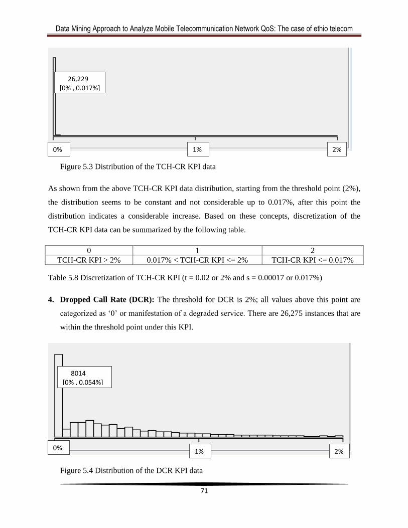
Data Mining Approach to Analyze Mobile Telecommunication Network QoS: The case of ethio telecom
71
Figure 5.3 Distribution of the TCH-CR KPI data
As shown from the above TCH-CR KPI data distribution, starting from the threshold point (2%),
the distribution seems to be constant and not considerable up to 0.017%, after this point the
distribution indicates a considerable increase. Based on these concepts, discretization of the
TCH-CR KPI data can be summarized by the following table.
0 1 2
TCH-CR KPI > 2% 0.017% < TCH-CR KPI <= 2% TCH-CR KPI <= 0.017%
Table 5.8 Discretization of TCH-CR KPI (t = 0.02 or 2% and s = 0.00017 or 0.017%)
4. Dropped Call Rate (DCR): The threshold for DCR is 2%; all values above this point are
categorized as ‗0‘ or manifestation of a degraded service. There are 26,275 instances that are
within the threshold point under this KPI.
Figure 5.4 Distribution of the DCR KPI data
26,229 [0% , 0.017%]
8014 [0% , 0.054%]
2% 1% 0%
2% 1% 0%
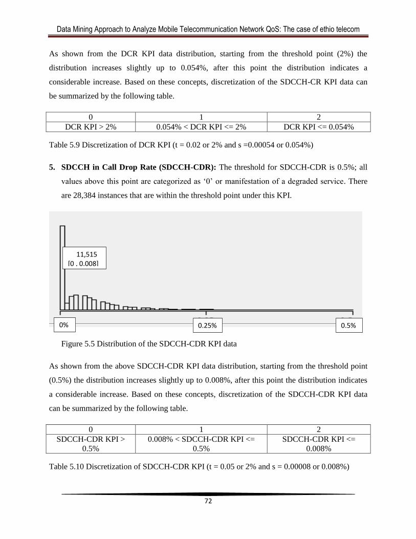
Data Mining Approach to Analyze Mobile Telecommunication Network QoS: The case of ethio telecom
72
As shown from the DCR KPI data distribution, starting from the threshold point (2%) the
distribution increases slightly up to 0.054%, after this point the distribution indicates a
considerable increase. Based on these concepts, discretization of the SDCCH-CR KPI data can
be summarized by the following table.
0 1 2
DCR KPI > 2% 0.054% < DCR KPI <= 2% DCR KPI <= 0.054%
Table 5.9 Discretization of DCR KPI (t = 0.02 or 2% and s =0.00054 or 0.054%)
5. SDCCH in Call Drop Rate (SDCCH-CDR): The threshold for SDCCH-CDR is 0.5%; all
values above this point are categorized as ‗0‘ or manifestation of a degraded service. There
are 28,384 instances that are within the threshold point under this KPI.
Figure 5.5 Distribution of the SDCCH-CDR KPI data
As shown from the above SDCCH-CDR KPI data distribution, starting from the threshold point
(0.5%) the distribution increases slightly up to 0.008%, after this point the distribution indicates
a considerable increase. Based on these concepts, discretization of the SDCCH-CDR KPI data
can be summarized by the following table.
0 1 2
SDCCH-CDR KPI >
0.5%
0.008% < SDCCH-CDR KPI <=
0.5%
SDCCH-CDR KPI <=
0.008%
Table 5.10 Discretization of SDCCH-CDR KPI (t = 0.05 or 2% and s = 0.00008 or 0.008%)
11,515 [0 , 0.008]
0.5% 0% 0.25%
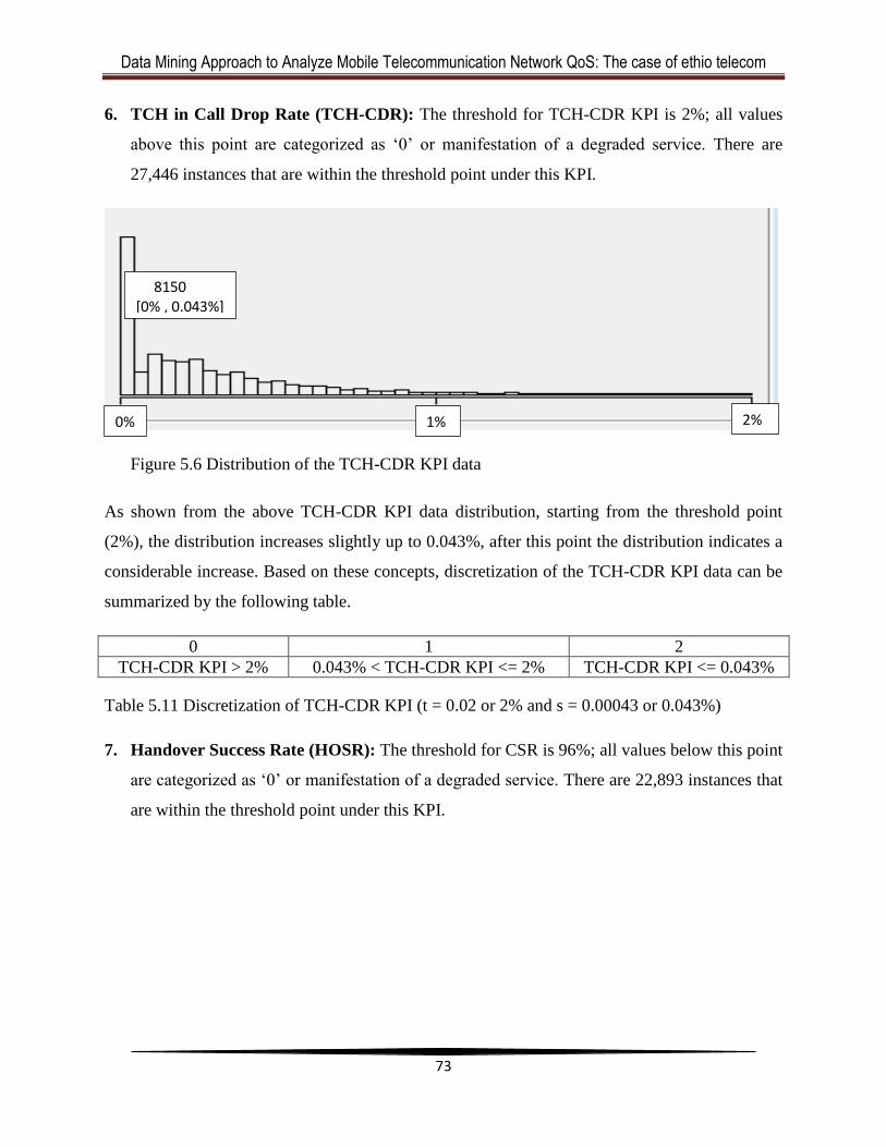
Data Mining Approach to Analyze Mobile Telecommunication Network QoS: The case of ethio telecom
73
6. TCH in Call Drop Rate (TCH-CDR): The threshold for TCH-CDR KPI is 2%; all values
above this point are categorized as ‗0‘ or manifestation of a degraded service. There are
27,446 instances that are within the threshold point under this KPI.
Figure 5.6 Distribution of the TCH-CDR KPI data
As shown from the above TCH-CDR KPI data distribution, starting from the threshold point
(2%), the distribution increases slightly up to 0.043%, after this point the distribution indicates a
considerable increase. Based on these concepts, discretization of the TCH-CDR KPI data can be
summarized by the following table.
0 1 2
TCH-CDR KPI > 2% 0.043% < TCH-CDR KPI <= 2% TCH-CDR KPI <= 0.043%
Table 5.11 Discretization of TCH-CDR KPI (t = 0.02 or 2% and s = 0.00043 or 0.043%)
7. Handover Success Rate (HOSR): The threshold for CSR is 96%; all values below this point
are categorized as ‗0‘ or manifestation of a degraded service. There are 22,893 instances that
are within the threshold point under this KPI.
8150 [0% , 0.043%]
2% 1% 0%
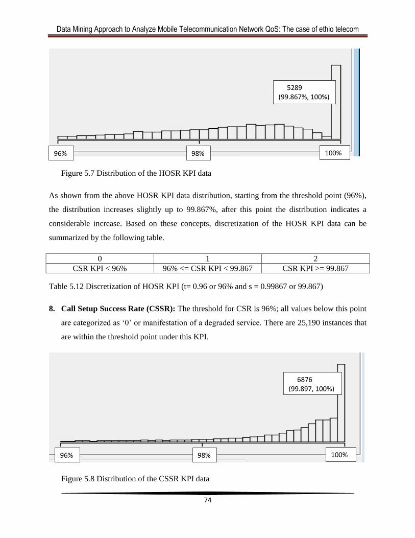
Data Mining Approach to Analyze Mobile Telecommunication Network QoS: The case of ethio telecom
74
Figure 5.7 Distribution of the HOSR KPI data
As shown from the above HOSR KPI data distribution, starting from the threshold point (96%),
the distribution increases slightly up to 99.867%, after this point the distribution indicates a
considerable increase. Based on these concepts, discretization of the HOSR KPI data can be
summarized by the following table.
0 1 2
CSR KPI < 96% 96% <= CSR KPI < 99.867 CSR KPI >= 99.867
Table 5.12 Discretization of HOSR KPI (t= 0.96 or 96% and s = 0.99867 or 99.867)
8. Call Setup Success Rate (CSSR): The threshold for CSR is 96%; all values below this point
are categorized as ‗0‘ or manifestation of a degraded service. There are 25,190 instances that
are within the threshold point under this KPI.
Figure 5.8 Distribution of the CSSR KPI data
5289 (99.867%, 100%)
6876 (99.897, 100%)
98% 96% 100%
98% 96% 100%
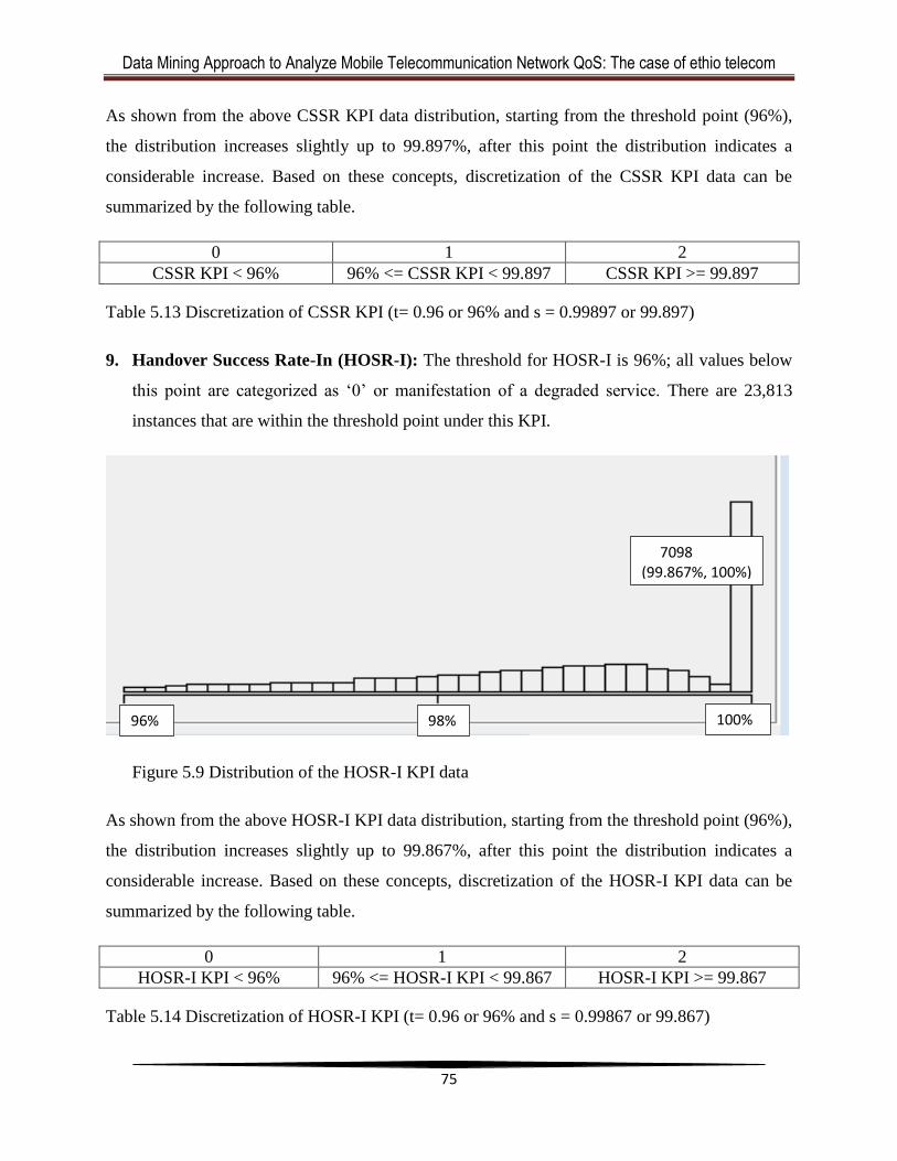
Data Mining Approach to Analyze Mobile Telecommunication Network QoS: The case of ethio telecom
75
As shown from the above CSSR KPI data distribution, starting from the threshold point (96%),
the distribution increases slightly up to 99.897%, after this point the distribution indicates a
considerable increase. Based on these concepts, discretization of the CSSR KPI data can be
summarized by the following table.
0 1 2
CSSR KPI < 96% 96% <= CSSR KPI < 99.897 CSSR KPI >= 99.897
Table 5.13 Discretization of CSSR KPI (t= 0.96 or 96% and s = 0.99897 or 99.897)
9. Handover Success Rate-In (HOSR-I): The threshold for HOSR-I is 96%; all values below
this point are categorized as ‗0‘ or manifestation of a degraded service. There are 23,813
instances that are within the threshold point under this KPI.
Figure 5.9 Distribution of the HOSR-I KPI data
As shown from the above HOSR-I KPI data distribution, starting from the threshold point (96%),
the distribution increases slightly up to 99.867%, after this point the distribution indicates a
considerable increase. Based on these concepts, discretization of the HOSR-I KPI data can be
summarized by the following table.
0 1 2
HOSR-I KPI < 96% 96% <= HOSR-I KPI < 99.867 HOSR-I KPI >= 99.867
Table 5.14 Discretization of HOSR-I KPI (t= 0.96 or 96% and s = 0.99867 or 99.867)
7098 (99.867%, 100%)
98% 96% 100%
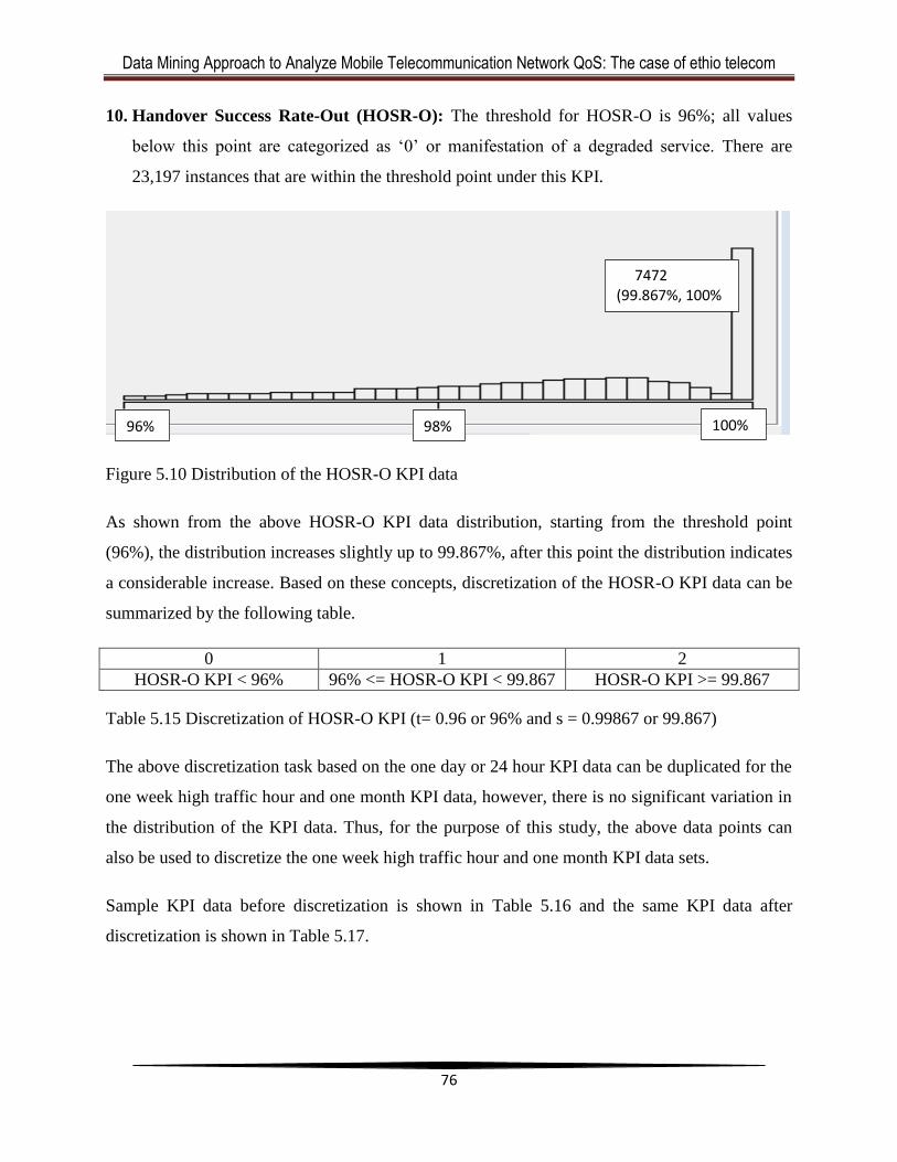
Data Mining Approach to Analyze Mobile Telecommunication Network QoS: The case of ethio telecom
76
10. Handover Success Rate-Out (HOSR-O): The threshold for HOSR-O is 96%; all values
below this point are categorized as ‗0‘ or manifestation of a degraded service. There are
23,197 instances that are within the threshold point under this KPI.
Figure 5.10 Distribution of the HOSR-O KPI data
As shown from the above HOSR-O KPI data distribution, starting from the threshold point
(96%), the distribution increases slightly up to 99.867%, after this point the distribution indicates
a considerable increase. Based on these concepts, discretization of the HOSR-O KPI data can be
summarized by the following table.
0 1 2
HOSR-O KPI < 96% 96% <= HOSR-O KPI < 99.867 HOSR-O KPI >= 99.867
Table 5.15 Discretization of HOSR-O KPI (t= 0.96 or 96% and s = 0.99867 or 99.867)
The above discretization task based on the one day or 24 hour KPI data can be duplicated for the
one week high traffic hour and one month KPI data, however, there is no significant variation in
the distribution of the KPI data. Thus, for the purpose of this study, the above data points can
also be used to discretize the one week high traffic hour and one month KPI data sets.
Sample KPI data before discretization is shown in Table 5.16 and the same KPI data after
discretization is shown in Table 5.17.
7472 (99.867%, 100%
98% 96% 100%
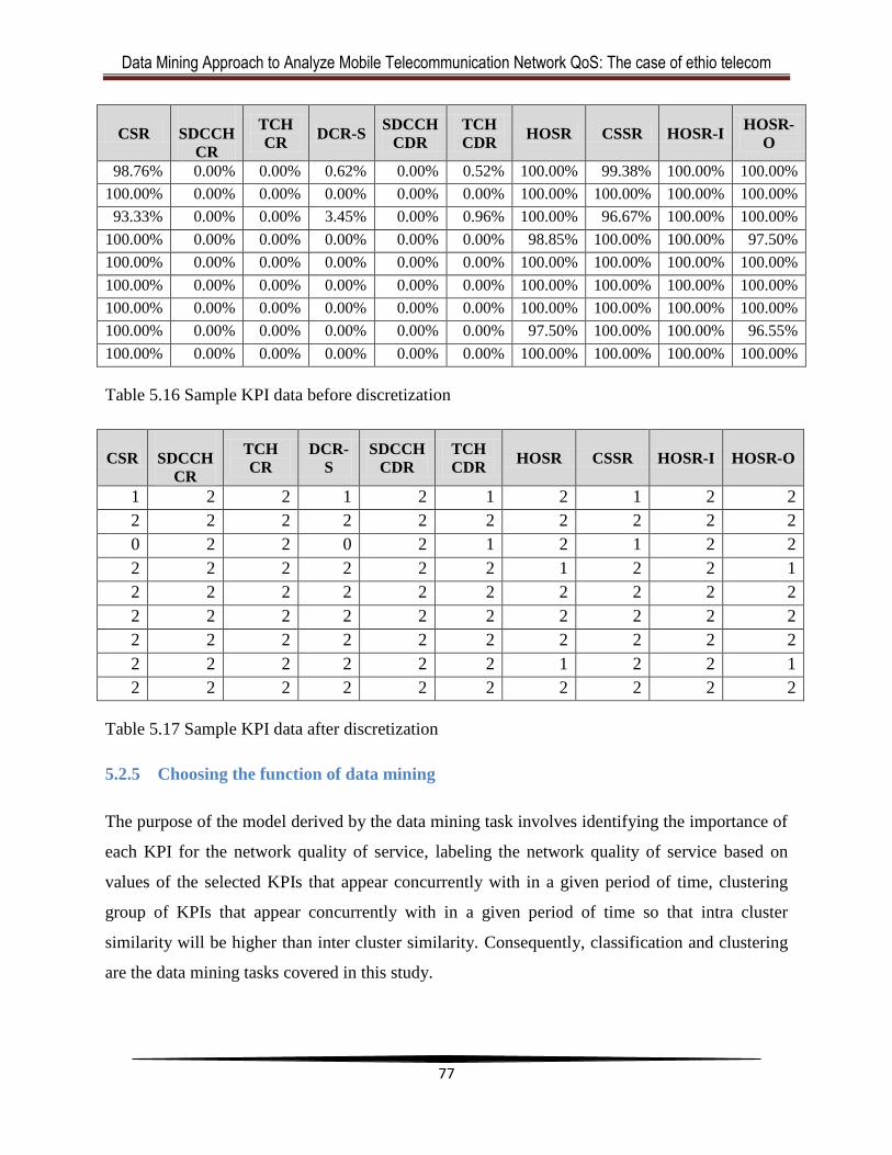
Data Mining Approach to Analyze Mobile Telecommunication Network QoS: The case of ethio telecom
77
CSR
SDCCH
CR
TCH
CR DCR-S
SDCCH
CDR
TCH
CDR HOSR CSSR HOSR-I
HOSR-
O
98.76% 0.00% 0.00% 0.62% 0.00% 0.52% 100.00% 99.38% 100.00% 100.00%
100.00% 0.00% 0.00% 0.00% 0.00% 0.00% 100.00% 100.00% 100.00% 100.00%
93.33% 0.00% 0.00% 3.45% 0.00% 0.96% 100.00% 96.67% 100.00% 100.00%
100.00% 0.00% 0.00% 0.00% 0.00% 0.00% 98.85% 100.00% 100.00% 97.50%
100.00% 0.00% 0.00% 0.00% 0.00% 0.00% 100.00% 100.00% 100.00% 100.00%
100.00% 0.00% 0.00% 0.00% 0.00% 0.00% 100.00% 100.00% 100.00% 100.00%
100.00% 0.00% 0.00% 0.00% 0.00% 0.00% 100.00% 100.00% 100.00% 100.00%
100.00% 0.00% 0.00% 0.00% 0.00% 0.00% 97.50% 100.00% 100.00% 96.55%
100.00% 0.00% 0.00% 0.00% 0.00% 0.00% 100.00% 100.00% 100.00% 100.00%
Table 5.16 Sample KPI data before discretization
CSR
SDCCH
CR
TCH
CR
DCR-
S
SDCCH
CDR
TCH
CDR HOSR CSSR HOSR-I HOSR-O
1 2 2 1 2 1 2 1 2 2
2 2 2 2 2 2 2 2 2 2
0 2 2 0 2 1 2 1 2 2
2 2 2 2 2 2 1 2 2 1
2 2 2 2 2 2 2 2 2 2
2 2 2 2 2 2 2 2 2 2
2 2 2 2 2 2 2 2 2 2
2 2 2 2 2 2 1 2 2 1
2 2 2 2 2 2 2 2 2 2
Table 5.17 Sample KPI data after discretization
5.2.5 Choosing the function of data mining
The purpose of the model derived by the data mining task involves identifying the importance of
each KPI for the network quality of service, labeling the network quality of service based on
values of the selected KPIs that appear concurrently with in a given period of time, clustering
group of KPIs that appear concurrently with in a given period of time so that intra cluster
similarity will be higher than inter cluster similarity. Consequently, classification and clustering
are the data mining tasks covered in this study.
Data Mining Approach to Analyze Mobile Telecommunication Network QoS: The case of ethio telecom
78
5.2.6 Choosing the data mining algorithm
The data mining algorithms selected for the tasks on this study such as classification, and
clustering are covered in chapter 4. For, classification, J48 decision tree algorithm, Naïve Bayes
and multilayer perception, and for clustering, k-means algorithms are applied. These algorithms
become best matches for this study not only by their pros and cons described previously but also
by different experimentations undertaken to choose the best algorithm per each data mining task.
5.2.7 Data Mining
After having the final data set at hand, the next task will be data mining. As indicated in Witten
et.al. (2011), the final data set prepared for the data mining task doesn‘t specify which one of the
attributes is going to be predicted. Thus, the same data set can be used to predict each attribute
from the others in the case of classification, or to find association rules, or for clustering. In this
regard, the data set of this study does not include a class label up to this point that aggregates
each instances of the KPI.
On the other hand, Witten et. al. (2011) also discuss that when there is no specified class,
clustering can be used to group items based on the natural proximity of the data. It may be
followed by a second step of classification learning in which rules are learned regarding how
new instances should be placed into the clusters. Likewise, after the first clustering
experimentation, the classification task will be preceded by the class labeling.
As indicated from the outset, there are three data sets extracted from the network management
system database, all of them are cleansed and reduced for the actual data mining task. After the
preprocessing stage, the one day or 24 hour KPI data set contains 28,680 instances per each KPI
(averaged per one hour granularity), the one week busy hour KPI data set contains 16,899
instances per each KPI (averaged per one hour granularity), and the one month KPI data set
contains 37,510 instances per each KPI (averaged per one day granularity). Finally, all these data
sets are consolidated in to one data set that contains 83,089 instances per each KPI.
In order to increase the representativeness of the data set, as much care as possible should be
taken when samples are selected. In this regard, due to the nature of the application area, not only
the effect of each KPI with in one full day or 24 hour should be visualized but also the
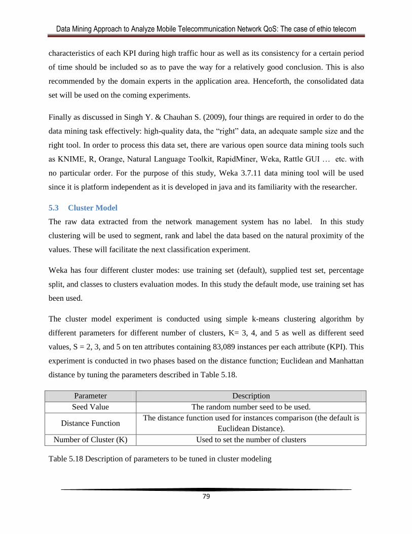
Data Mining Approach to Analyze Mobile Telecommunication Network QoS: The case of ethio telecom
79
characteristics of each KPI during high traffic hour as well as its consistency for a certain period
of time should be included so as to pave the way for a relatively good conclusion. This is also
recommended by the domain experts in the application area. Henceforth, the consolidated data
set will be used on the coming experiments.
Finally as discussed in Singh Y. & Chauhan S. (2009), four things are required in order to do the
data mining task effectively: high-quality data, the ―right‖ data, an adequate sample size and the
right tool. In order to process this data set, there are various open source data mining tools such
as KNIME, R, Orange, Natural Language Toolkit, RapidMiner, Weka, Rattle GUI … etc. with
no particular order. For the purpose of this study, Weka 3.7.11 data mining tool will be used
since it is platform independent as it is developed in java and its familiarity with the researcher.
5.3 Cluster Model
The raw data extracted from the network management system has no label. In this study
clustering will be used to segment, rank and label the data based on the natural proximity of the
values. These will facilitate the next classification experiment.
Weka has four different cluster modes: use training set (default), supplied test set, percentage
split, and classes to clusters evaluation modes. In this study the default mode, use training set has
been used.
The cluster model experiment is conducted using simple k-means clustering algorithm by
different parameters for different number of clusters, K= 3, 4, and 5 as well as different seed
values, S = 2, 3, and 5 on ten attributes containing 83,089 instances per each attribute (KPI). This
experiment is conducted in two phases based on the distance function; Euclidean and Manhattan
distance by tuning the parameters described in Table 5.18.
Parameter Description
Seed Value The random number seed to be used.
Distance Function The distance function used for instances comparison (the default is
Euclidean Distance).
Number of Cluster (K) Used to set the number of clusters
Table 5.18 Description of parameters to be tuned in cluster modeling
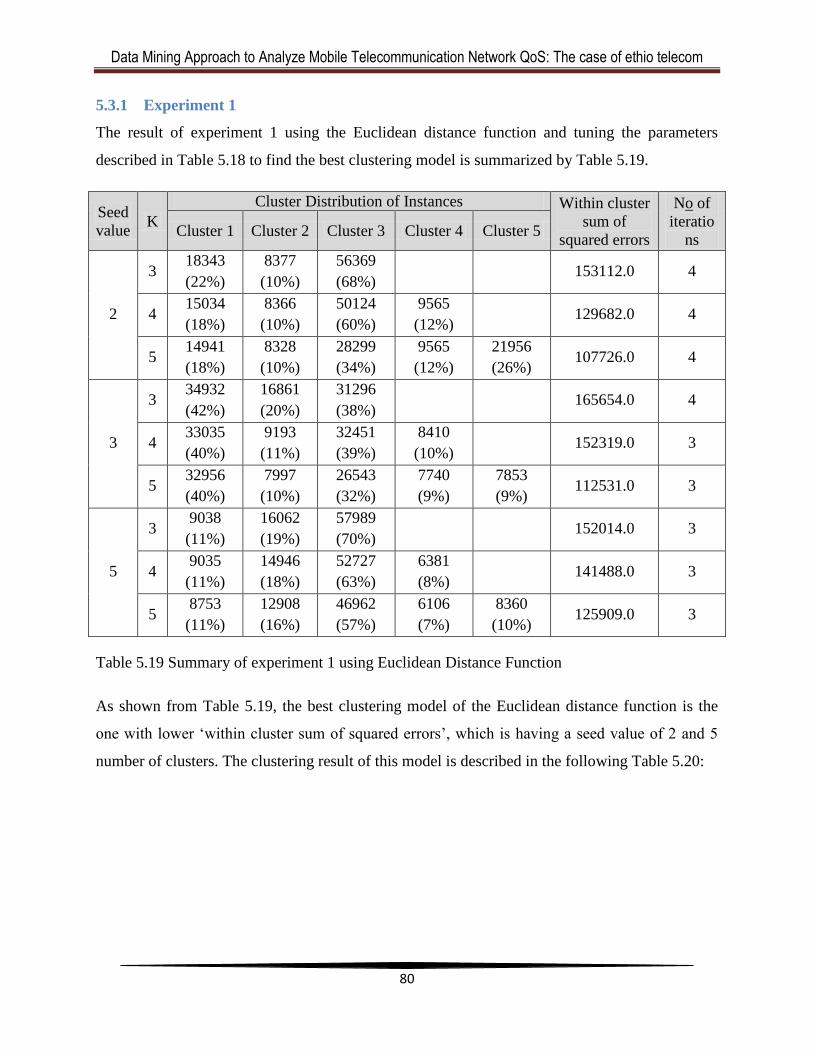
Data Mining Approach to Analyze Mobile Telecommunication Network QoS: The case of ethio telecom
80
5.3.1 Experiment 1
The result of experiment 1 using the Euclidean distance function and tuning the parameters
described in Table 5.18 to find the best clustering model is summarized by Table 5.19.
Seed
value K
Cluster Distribution of Instances Within cluster
sum of
squared errors
No of
iteratio
ns Cluster 1 Cluster 2 Cluster 3 Cluster 4 Cluster 5
2
3 18343
(22%)
8377
(10%)
56369
(68%) 153112.0 4
4 15034
(18%)
8366
(10%)
50124
(60%)
9565
(12%) 129682.0 4
5 14941
(18%)
8328
(10%)
28299
(34%)
9565
(12%)
21956
(26%) 107726.0 4
3
3 34932
(42%)
16861
(20%)
31296
(38%) 165654.0 4
4 33035
(40%)
9193
(11%)
32451
(39%)
8410
(10%) 152319.0 3
5 32956
(40%)
7997
(10%)
26543
(32%)
7740
(9%)
7853
(9%) 112531.0 3
5
3 9038
(11%)
16062
(19%)
57989
(70%) 152014.0 3
4 9035
(11%)
14946
(18%)
52727
(63%)
6381
(8%) 141488.0 3
5 8753
(11%)
12908
(16%)
46962
(57%)
6106
(7%)
8360
(10%) 125909.0 3
Table 5.19 Summary of experiment 1 using Euclidean Distance Function
As shown from Table 5.19, the best clustering model of the Euclidean distance function is the
one with lower ‗within cluster sum of squared errors‘, which is having a seed value of 2 and 5
number of clusters. The clustering result of this model is described in the following Table 5.20:
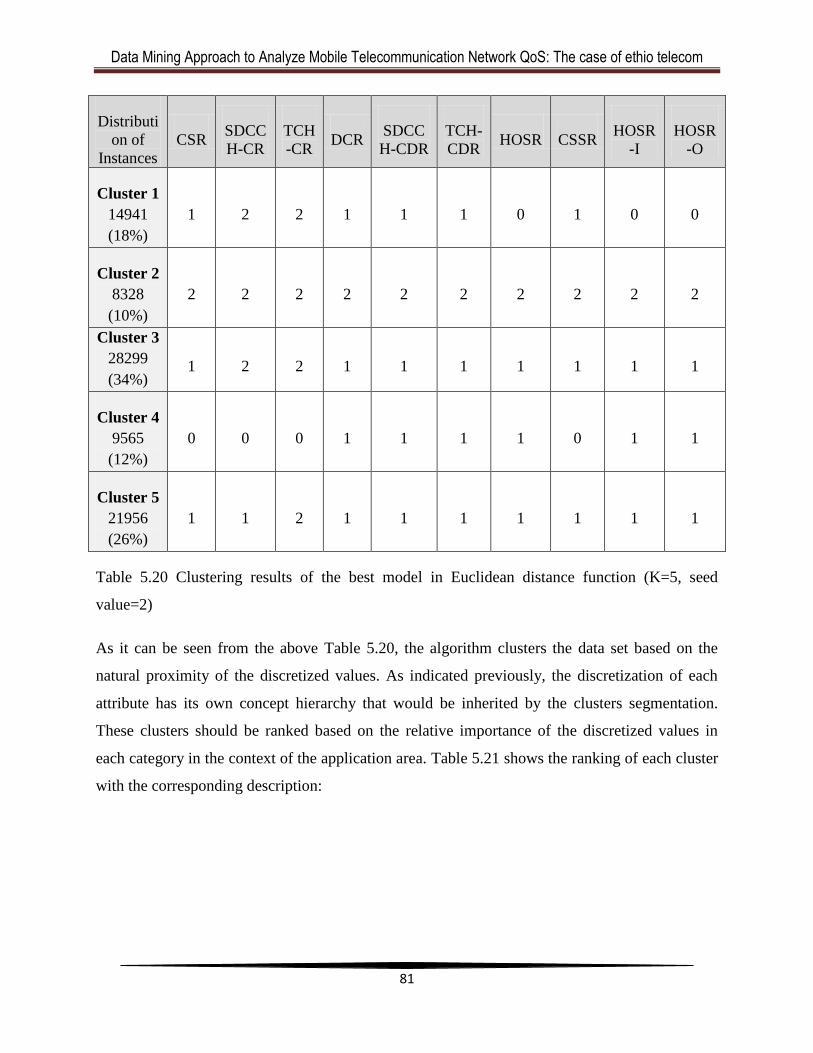
Data Mining Approach to Analyze Mobile Telecommunication Network QoS: The case of ethio telecom
81
Distributi
on of
Instances
CSR SDCC
H-CR
TCH
-CR DCR
SDCC
H-CDR
TCH-
CDR HOSR CSSR
HOSR
-I
HOSR
-O
Cluster 1
14941
(18%)
1 2 2 1 1 1 0 1 0 0
Cluster 2
8328
(10%)
2 2 2 2 2 2 2 2 2 2
Cluster 3
28299
(34%) 1 2 2 1 1 1 1 1 1 1
Cluster 4
9565
(12%)
0 0 0 1 1 1 1 0 1 1
Cluster 5
21956
(26%)
1 1 2 1 1 1 1 1 1 1
Table 5.20 Clustering results of the best model in Euclidean distance function (K=5, seed
value=2)
As it can be seen from the above Table 5.20, the algorithm clusters the data set based on the
natural proximity of the discretized values. As indicated previously, the discretization of each
attribute has its own concept hierarchy that would be inherited by the clusters segmentation.
These clusters should be ranked based on the relative importance of the discretized values in
each category in the context of the application area. Table 5.21 shows the ranking of each cluster
with the corresponding description:
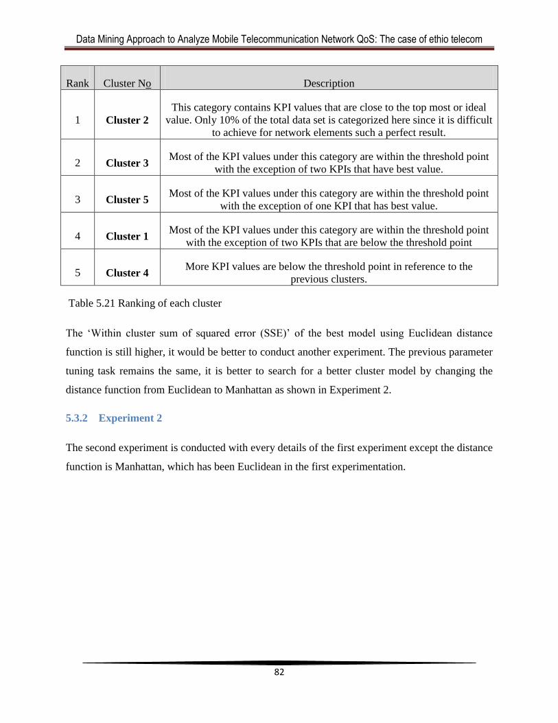
Data Mining Approach to Analyze Mobile Telecommunication Network QoS: The case of ethio telecom
82
Rank Cluster No Description
1 Cluster 2
This category contains KPI values that are close to the top most or ideal
value. Only 10% of the total data set is categorized here since it is difficult
to achieve for network elements such a perfect result.
2 Cluster 3 Most of the KPI values under this category are within the threshold point
with the exception of two KPIs that have best value.
3 Cluster 5 Most of the KPI values under this category are within the threshold point
with the exception of one KPI that has best value.
4 Cluster 1 Most of the KPI values under this category are within the threshold point
with the exception of two KPIs that are below the threshold point
5 Cluster 4 More KPI values are below the threshold point in reference to the
previous clusters.
Table 5.21 Ranking of each cluster
The ‗Within cluster sum of squared error (SSE)‘ of the best model using Euclidean distance
function is still higher, it would be better to conduct another experiment. The previous parameter
tuning task remains the same, it is better to search for a better cluster model by changing the
distance function from Euclidean to Manhattan as shown in Experiment 2.
5.3.2 Experiment 2
The second experiment is conducted with every details of the first experiment except the distance
function is Manhattan, which has been Euclidean in the first experimentation.
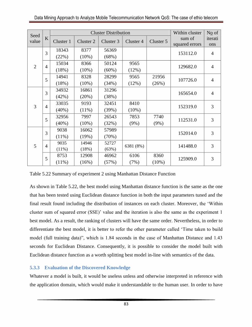
Data Mining Approach to Analyze Mobile Telecommunication Network QoS: The case of ethio telecom
83
Seed
value K
Cluster Distribution Within cluster
sum of
squared errors
No of
iterati
ons Cluster 1 Cluster 2 Cluster 3 Cluster 4 Cluster 5
2
3 18343
(22%)
8377
(10%)
56369
(68%) 153112.0 4
4 15034
(18%)
8366
(10%)
50124
(60%)
9565
(12%) 129682.0 4
5 14941
(18%)
8328
(10%)
28299
(34%)
9565
(12%)
21956
(26%) 107726.0 4
3
3 34932
(42%)
16861
(20%)
31296
(38%) 165654.0 4
4 33035
(40%)
9193
(11%)
32451
(39%)
8410
(10%) 152319.0 3
5 32956
(40%)
7997
(10%)
26543
(32%)
7853
(9%)
7740
(9%) 112531.0 3
5
3 9038
(11%)
16062
(19%)
57989
(70%) 152014.0 3
4 9035
(11%)
14946
(18%)
52727
(63%) 6381 (8%) 141488.0 3
5 8753
(11%)
12908
(16%)
46962
(57%)
6106
(7%)
8360
(10%) 125909.0 3
Table 5.22 Summary of experiment 2 using Manhattan Distance Function
As shown in Table 5.22, the best model using Manhattan distance function is the same as the one
that has been tested using Euclidean distance function in both the input parameters tuned and the
final result found including the distribution of instances on each cluster. Moreover, the ‗Within
cluster sum of squared error (SSE)‘ value and the iteration is also the same as the experiment 1
best model. As a result, the ranking of clusters will have the same order. Nevertheless, in order to
differentiate the best model, it is better to refer the other parameter called ‗Time taken to build
model (full training data)‖, which is 1.84 seconds in the case of Manhattan Distance and 1.43
seconds for Euclidean Distance. Consequently, it is possible to consider the model built with
Euclidean distance function as a worth splitting best model in-line with semantics of the data.
5.3.3 Evaluation of the Discovered Knowledge
Whatever a model is built, it would be useless unless and otherwise interpreted in reference with
the application domain, which would make it understandable to the human user. In order to have
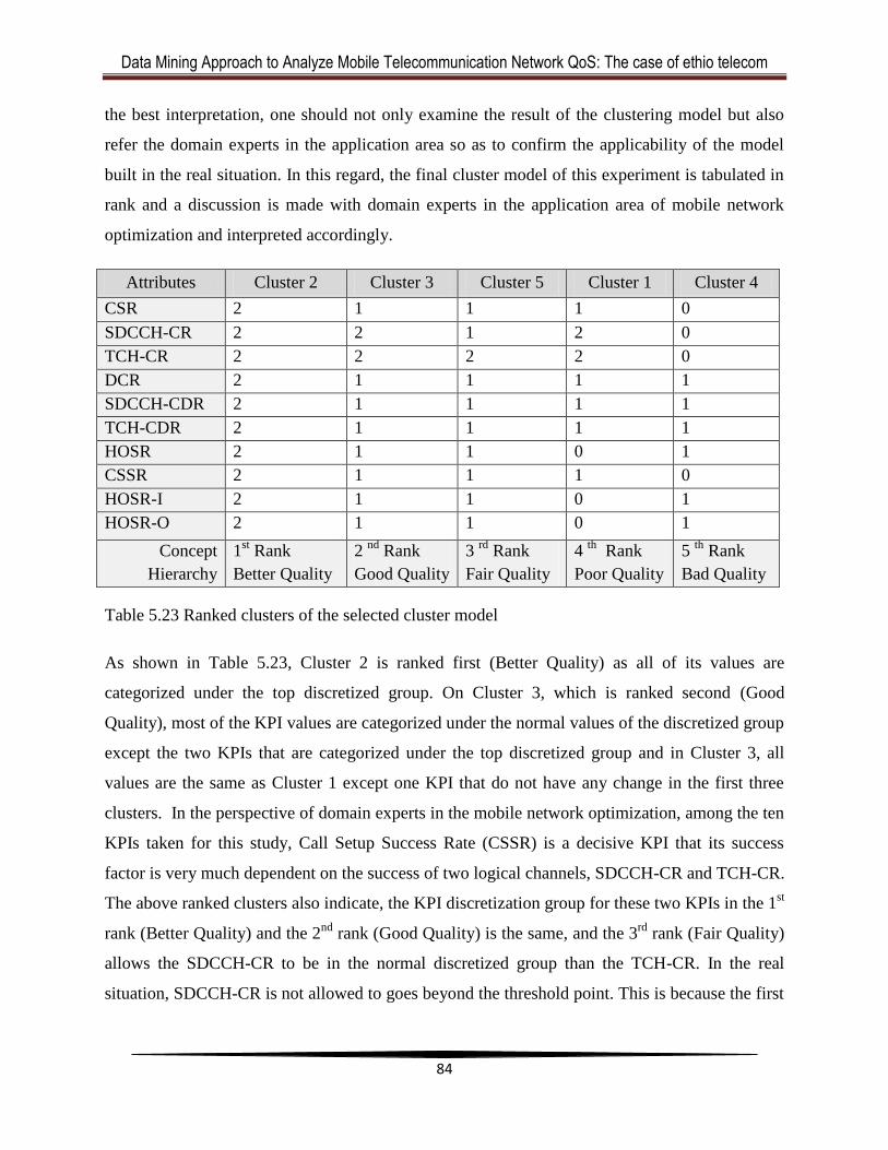
Data Mining Approach to Analyze Mobile Telecommunication Network QoS: The case of ethio telecom
84
the best interpretation, one should not only examine the result of the clustering model but also
refer the domain experts in the application area so as to confirm the applicability of the model
built in the real situation. In this regard, the final cluster model of this experiment is tabulated in
rank and a discussion is made with domain experts in the application area of mobile network
optimization and interpreted accordingly.
Attributes Cluster 2 Cluster 3 Cluster 5 Cluster 1 Cluster 4
CSR 2 1 1 1 0
SDCCH-CR 2 2 1 2 0
TCH-CR 2 2 2 2 0
DCR 2 1 1 1 1
SDCCH-CDR 2 1 1 1 1
TCH-CDR 2 1 1 1 1
HOSR 2 1 1 0 1
CSSR 2 1 1 1 0
HOSR-I 2 1 1 0 1
HOSR-O 2 1 1 0 1
Concept
Hierarchy
1st Rank
Better Quality
2 nd
Rank
Good Quality
3 rd
Rank
Fair Quality
4 th
Rank
Poor Quality
5 th
Rank
Bad Quality
Table 5.23 Ranked clusters of the selected cluster model
As shown in Table 5.23, Cluster 2 is ranked first (Better Quality) as all of its values are
categorized under the top discretized group. On Cluster 3, which is ranked second (Good
Quality), most of the KPI values are categorized under the normal values of the discretized group
except the two KPIs that are categorized under the top discretized group and in Cluster 3, all
values are the same as Cluster 1 except one KPI that do not have any change in the first three
clusters. In the perspective of domain experts in the mobile network optimization, among the ten
KPIs taken for this study, Call Setup Success Rate (CSSR) is a decisive KPI that its success
factor is very much dependent on the success of two logical channels, SDCCH-CR and TCH-CR.
The above ranked clusters also indicate, the KPI discretization group for these two KPIs in the 1st
rank (Better Quality) and the 2nd
rank (Good Quality) is the same, and the 3rd
rank (Fair Quality)
allows the SDCCH-CR to be in the normal discretized group than the TCH-CR. In the real
situation, SDCCH-CR is not allowed to goes beyond the threshold point. This is because the first
Data Mining Approach to Analyze Mobile Telecommunication Network QoS: The case of ethio telecom
85
resource that should be allocated for a subscriber is SDCCH since it is mandatory for call
establishment, so that it should be available even in a very congested network environment.
If there is a considerable deviation between the CSR and the CSSR, it is an indication of a
remarkable DCR so that the KPI value for CSR should not deviate much from the CSSR. In
reference with the best cluster model selected, the CSSR value from rank 1 to rank 5 is 2,1,1,1,0
respectively and that of CSR is the same as the CSSR, which is 2,1,1,1,0. This shows the value
of CSSR and CSR with in the same cluster have a value that fall under the same discretized
group, which indicates the KPI values of CSSR and CSR are consistent in their respective
cluster.
In the 4th
ranked cluster (Poor Quality), HOSR, HOSR-I, and HOSR-O are beyond the threshold
limit, however the rest KPIs in this cluster are within the desired range. In the 5th
ranked cluster
(Bad Quality), SDCCH-CR, TCH-CR, CSSR and the CSR are under the threshold point. What
makes the 4th
ranked cluster better than the 5th
ranked cluster is that it only affects the HOSR
KPIs that are related to the mobility nature of the network. In other words, the fourth ranked
cluster only affects the moving customers but normal for the rest. In the 5th
ranked cluster the
negative impact on SDCCH-CR and TCH-CR affects the value of CSSR which in turns affect
the value of the CSR. This will again confirms the dependency of CSSR on the values of
SDCCH-CR and TCH-CR as described previously.
5.4 Classification Model
In the previous experiments, the best cluster model is selected and examined with the domain
experts‘ knowledge in the application area. It would be logical to consider the cluster
categorization created by this clustering model for the experimentation of the classification
model, since the model worth splits the data set based on its natural proximity.
In this study, experimentation of classification model is conducted using three different
algorithms: J48 decision tree classifier, Naïve Bayes classifier, and multilayer perception
classifier. These algorithms are experimented by tuning different parameters in Weka to get the
best classification model that can best classify the unseen data. Thus, randomly extracted and
preprocessed separate data sets of 8478 instances to train and test the model and 4240 instances
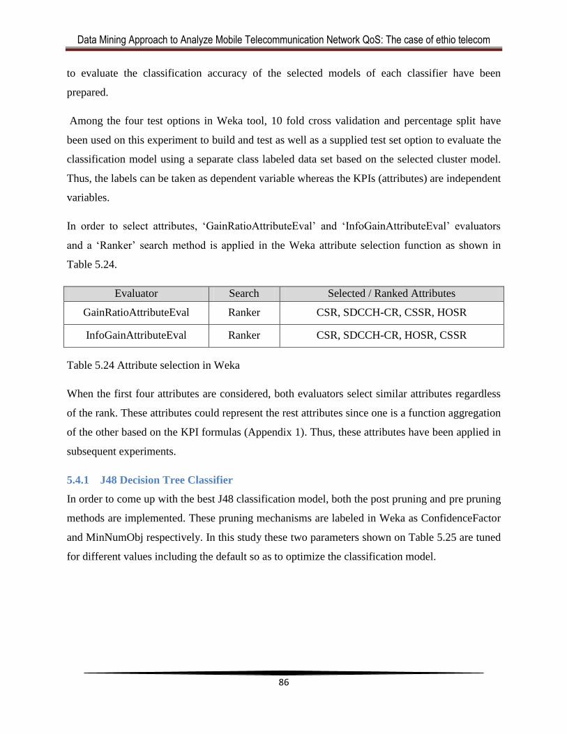
Data Mining Approach to Analyze Mobile Telecommunication Network QoS: The case of ethio telecom
86
to evaluate the classification accuracy of the selected models of each classifier have been
prepared.
Among the four test options in Weka tool, 10 fold cross validation and percentage split have
been used on this experiment to build and test as well as a supplied test set option to evaluate the
classification model using a separate class labeled data set based on the selected cluster model.
Thus, the labels can be taken as dependent variable whereas the KPIs (attributes) are independent
variables.
In order to select attributes, ‗GainRatioAttributeEval‘ and ‗InfoGainAttributeEval‘ evaluators
and a ‗Ranker‘ search method is applied in the Weka attribute selection function as shown in
Table 5.24.
Evaluator Search Selected / Ranked Attributes
GainRatioAttributeEval Ranker CSR, SDCCH-CR, CSSR, HOSR
InfoGainAttributeEval Ranker CSR, SDCCH-CR, HOSR, CSSR
Table 5.24 Attribute selection in Weka
When the first four attributes are considered, both evaluators select similar attributes regardless
of the rank. These attributes could represent the rest attributes since one is a function aggregation
of the other based on the KPI formulas (Appendix 1). Thus, these attributes have been applied in
subsequent experiments.
5.4.1 J48 Decision Tree Classifier
In order to come up with the best J48 classification model, both the post pruning and pre pruning
methods are implemented. These pruning mechanisms are labeled in Weka as ConfidenceFactor
and MinNumObj respectively. In this study these two parameters shown on Table 5.25 are tuned
for different values including the default so as to optimize the classification model.
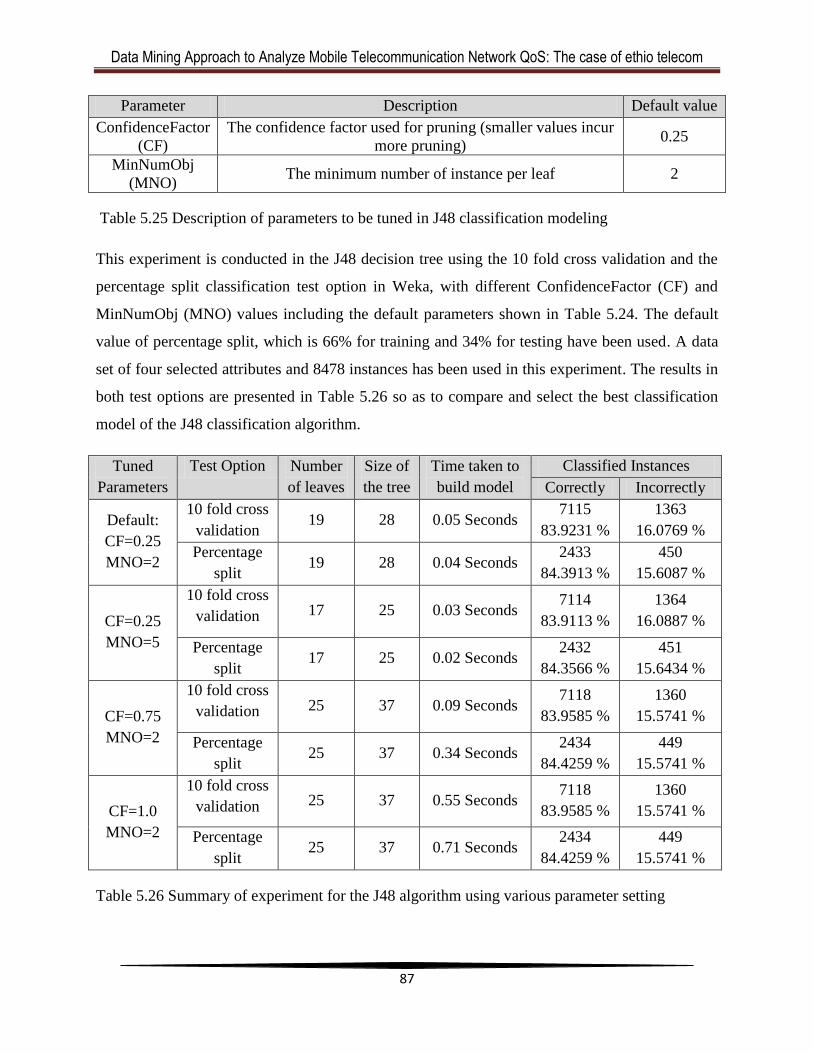
Data Mining Approach to Analyze Mobile Telecommunication Network QoS: The case of ethio telecom
87
Parameter Description Default value
ConfidenceFactor
(CF)
The confidence factor used for pruning (smaller values incur
more pruning) 0.25
MinNumObj
(MNO) The minimum number of instance per leaf 2
Table 5.25 Description of parameters to be tuned in J48 classification modeling
This experiment is conducted in the J48 decision tree using the 10 fold cross validation and the
percentage split classification test option in Weka, with different ConfidenceFactor (CF) and
MinNumObj (MNO) values including the default parameters shown in Table 5.24. The default
value of percentage split, which is 66% for training and 34% for testing have been used. A data
set of four selected attributes and 8478 instances has been used in this experiment. The results in
both test options are presented in Table 5.26 so as to compare and select the best classification
model of the J48 classification algorithm.
Tuned
Parameters
Test Option Number
of leaves
Size of
the tree
Time taken to
build model
Classified Instances
Correctly Incorrectly
Default:
CF=0.25
MNO=2
10 fold cross
validation 19 28 0.05 Seconds
7115
83.9231 %
1363
16.0769 %
Percentage
split 19 28 0.04 Seconds
2433
84.3913 %
450
15.6087 %
CF=0.25
MNO=5
10 fold cross
validation 17 25 0.03 Seconds 7114
83.9113 %
1364
16.0887 %
Percentage
split 17 25 0.02 Seconds
2432
84.3566 %
451
15.6434 %
CF=0.75
MNO=2
10 fold cross
validation 25 37 0.09 Seconds 7118
83.9585 %
1360
15.5741 %
Percentage
split 25 37 0.34 Seconds
2434
84.4259 %
449
15.5741 %
CF=1.0
MNO=2
10 fold cross
validation 25 37 0.55 Seconds 7118
83.9585 %
1360
15.5741 %
Percentage
split 25 37 0.71 Seconds
2434
84.4259 %
449
15.5741 %
Table 5.26 Summary of experiment for the J48 algorithm using various parameter setting
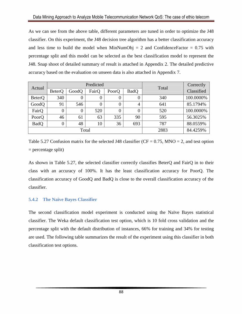
Data Mining Approach to Analyze Mobile Telecommunication Network QoS: The case of ethio telecom
88
As we can see from the above table, different parameters are tuned in order to optimize the J48
classifier. On this experiment, the J48 decision tree algorithm has a better classification accuracy
and less time to build the model when MinNumObj = 2 and ConfidenceFactor = 0.75 with
percentage split and this model can be selected as the best classification model to represent the
J48. Snap shoot of detailed summary of result is attached in Appendix 2. The detailed predictive
accuracy based on the evaluation on unseen data is also attached in Appendix 7.
Actual Predicted
Total Correctly
Classified BeterQ GoodQ FairQ PoorQ BadQ
BeterQ 340 0 0 0 0 340 100.0000%
GoodQ 91 546 0 0 4 641 85.1794%
FairQ 0 0 520 0 0 520 100.0000%
PoorQ 46 61 63 335 90 595 56.3025%
BadQ 0 48 10 36 693 787 88.0559%
Total 2883 84.4259%
Table 5.27 Confusion matrix for the selected J48 classifier (CF = 0.75, MNO = 2, and test option
= percentage split)
As shown in Table 5.27, the selected classifier correctly classifies BeterQ and FairQ in to their
class with an accuracy of 100%. It has the least classification accuracy for PoorQ. The
classification accuracy of GoodQ and BadQ is close to the overall classification accuracy of the
classifier.
5.4.2 The Naïve Bayes Classifier
The second classification model experiment is conducted using the Naïve Bayes statistical
classifier. The Weka default classification test option, which is 10 fold cross validation and the
percentage split with the default distribution of instances, 66% for training and 34% for testing
are used. The following table summarizes the result of the experiment using this classifier in both
classification test options.
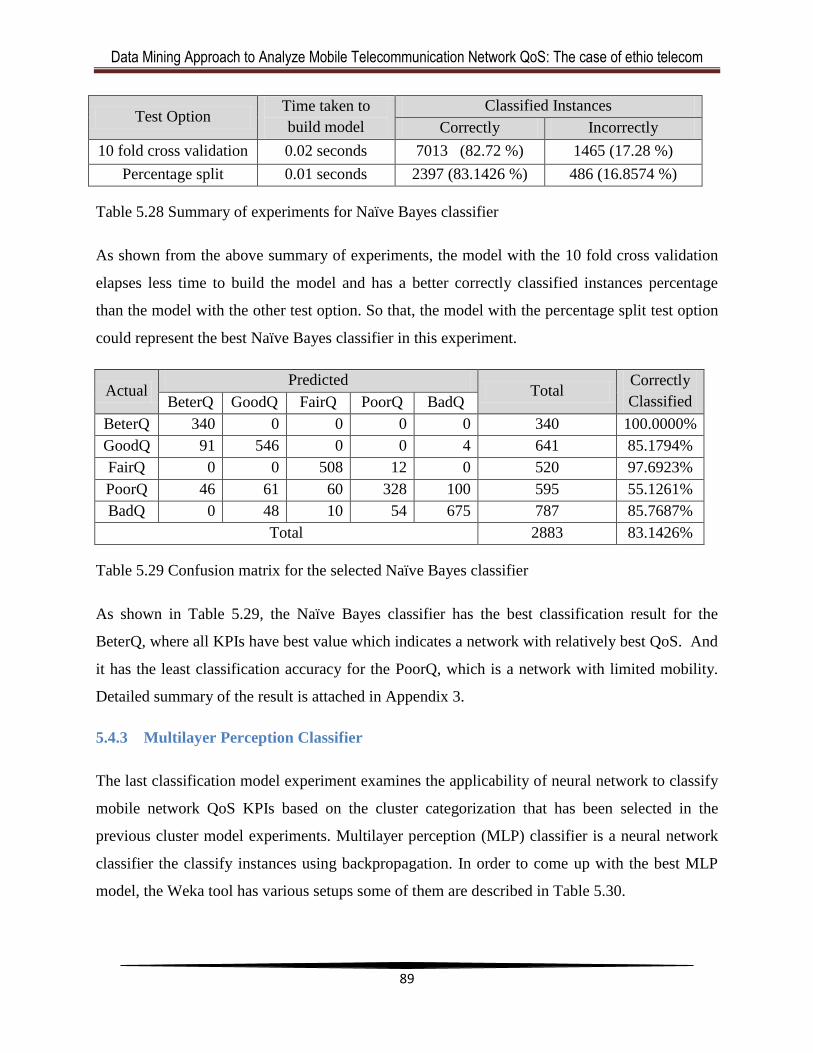
Data Mining Approach to Analyze Mobile Telecommunication Network QoS: The case of ethio telecom
89
Test Option Time taken to
build model
Classified Instances
Correctly Incorrectly
10 fold cross validation 0.02 seconds 7013 (82.72 %) 1465 (17.28 %)
Percentage split 0.01 seconds 2397 (83.1426 %) 486 (16.8574 %)
Table 5.28 Summary of experiments for Naïve Bayes classifier
As shown from the above summary of experiments, the model with the 10 fold cross validation
elapses less time to build the model and has a better correctly classified instances percentage
than the model with the other test option. So that, the model with the percentage split test option
could represent the best Naïve Bayes classifier in this experiment.
Actual Predicted
Total Correctly
Classified BeterQ GoodQ FairQ PoorQ BadQ
BeterQ 340 0 0 0 0 340 100.0000%
GoodQ 91 546 0 0 4 641 85.1794%
FairQ 0 0 508 12 0 520 97.6923%
PoorQ 46 61 60 328 100 595 55.1261%
BadQ 0 48 10 54 675 787 85.7687%
Total 2883 83.1426%
Table 5.29 Confusion matrix for the selected Naïve Bayes classifier
As shown in Table 5.29, the Naïve Bayes classifier has the best classification result for the
BeterQ, where all KPIs have best value which indicates a network with relatively best QoS. And
it has the least classification accuracy for the PoorQ, which is a network with limited mobility.
Detailed summary of the result is attached in Appendix 3.
5.4.3 Multilayer Perception Classifier
The last classification model experiment examines the applicability of neural network to classify
mobile network QoS KPIs based on the cluster categorization that has been selected in the
previous cluster model experiments. Multilayer perception (MLP) classifier is a neural network
classifier the classify instances using backpropagation. In order to come up with the best MLP
model, the Weka tool has various setups some of them are described in Table 5.30.
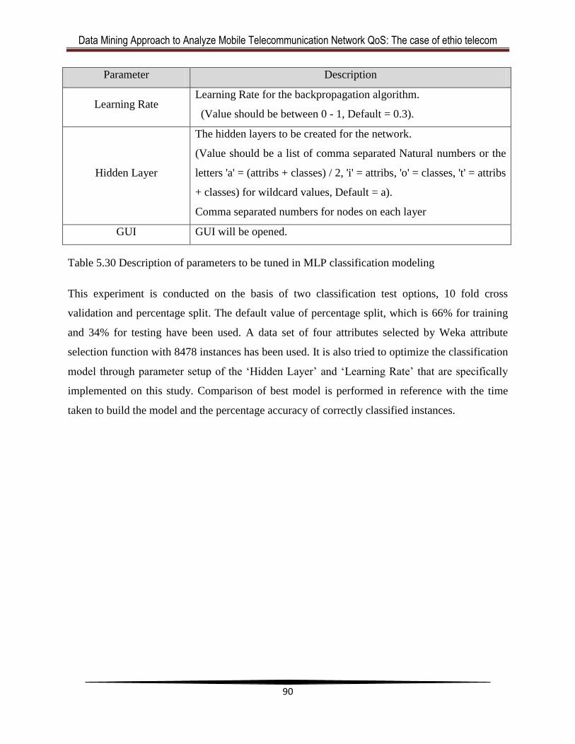
Data Mining Approach to Analyze Mobile Telecommunication Network QoS: The case of ethio telecom
90
Parameter Description
Learning Rate Learning Rate for the backpropagation algorithm.
(Value should be between 0 - 1, Default = 0.3).
Hidden Layer
The hidden layers to be created for the network.
(Value should be a list of comma separated Natural numbers or the
letters 'a' = (attribs + classes) / 2, 'i' = attribs, 'o' = classes, 't' = attribs
+ classes) for wildcard values, Default = a).
Comma separated numbers for nodes on each layer
GUI GUI will be opened.
Table 5.30 Description of parameters to be tuned in MLP classification modeling
This experiment is conducted on the basis of two classification test options, 10 fold cross
validation and percentage split. The default value of percentage split, which is 66% for training
and 34% for testing have been used. A data set of four attributes selected by Weka attribute
selection function with 8478 instances has been used. It is also tried to optimize the classification
model through parameter setup of the ‗Hidden Layer‘ and ‗Learning Rate‘ that are specifically
implemented on this study. Comparison of best model is performed in reference with the time
taken to build the model and the percentage accuracy of correctly classified instances.
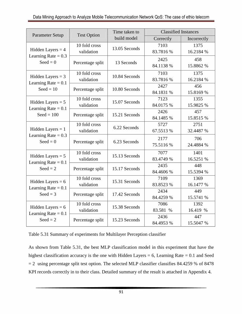
Data Mining Approach to Analyze Mobile Telecommunication Network QoS: The case of ethio telecom
91
Parameter Setup Test Option Time taken to
build model
Classified Instances
Correctly Incorrectly
Hidden Layers = 4
Learning Rate = 0.3
Seed = 0
10 fold cross
validation 13.05 Seconds
7103
83.7816 %
1375
16.2184 %
Percentage split 13 Seconds 2425
84.1138 %
458
15.8862 %
Hidden Layers = 3
Learning Rate = 0.1
Seed = 10
10 fold cross
validation 10.84 Seconds
7103
83.7816 %
1375
16.2184 %
Percentage split 10.80 Seconds 2427
84.1831 %
456
15.8169 %
Hidden Layers = 5
Learning Rate = 0.1
Seed = 100
10 fold cross
validation 15.07 Seconds
7123
84.0175 %
1355
15.9825 %
Percentage split 15.21 Seconds 2426
84.1485 %
457
15.8515 %
Hidden Layers = 1
Learning Rate = 0.3
Seed = 0
10 fold cross
validation 6.22 Seconds
5727
67.5513 %
2751
32.4487 %
Percentage split 6.23 Seconds 2177
75.5116 %
706
24.4884 %
Hidden Layers = 5
Learning Rate = 0.1
Seed = 2
10 fold cross
validation 15.13 Seconds
7077
83.4749 %
1401
16.5251 %
Percentage split 15.17 Seconds 2435
84.4606 %
448
15.5394 %
Hidden Layers = 6
Learning Rate = 0.1
Seed = 3
10 fold cross
validation 15.31 Seconds
7109
83.8523 %
1369
16.1477 %
Percentage split 17.42 Seconds 2434
84.4259 %
449
15.5741 %
Hidden Layers = 6
Learning Rate = 0.1
Seed = 2
10 fold cross
validation 15.38 Seconds
7086
83.581 %
1392
16.419 %
Percentage split 15.23 Seconds 2436
84.4953 %
447
15.5047 %
Table 5.31 Summary of experiments for Multilayer Perception classifier
As shown from Table 5.31, the best MLP classification model in this experiment that have the
highest classification accuracy is the one with Hidden Layers = 6, Learning Rate = 0.1 and Seed
= 2 using percentage split test option. The selected MLP classifier classifies 84.4259 % of 8478
KPI records correctly in to their class. Detailed summary of the result is attached in Appendix 4.
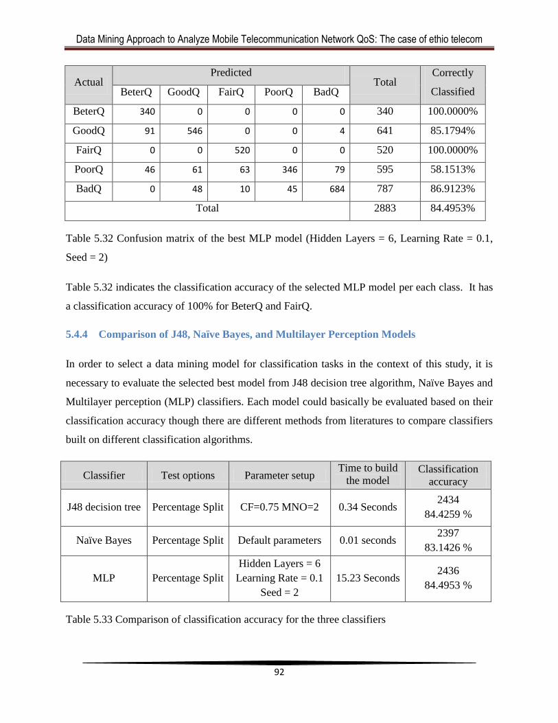
Data Mining Approach to Analyze Mobile Telecommunication Network QoS: The case of ethio telecom
92
Actual Predicted
Total Correctly
Classified BeterQ GoodQ FairQ PoorQ BadQ
BeterQ 340 0 0 0 0 340 100.0000%
GoodQ 91 546 0 0 4 641 85.1794%
FairQ 0 0 520 0 0 520 100.0000%
PoorQ 46 61 63 346 79 595 58.1513%
BadQ 0 48 10 45 684 787 86.9123%
Total 2883 84.4953%
Table 5.32 Confusion matrix of the best MLP model (Hidden Layers = 6, Learning Rate = 0.1,
Seed = 2)
Table 5.32 indicates the classification accuracy of the selected MLP model per each class. It has
a classification accuracy of 100% for BeterQ and FairQ.
5.4.4 Comparison of J48, Naïve Bayes, and Multilayer Perception Models
In order to select a data mining model for classification tasks in the context of this study, it is
necessary to evaluate the selected best model from J48 decision tree algorithm, Naïve Bayes and
Multilayer perception (MLP) classifiers. Each model could basically be evaluated based on their
classification accuracy though there are different methods from literatures to compare classifiers
built on different classification algorithms.
Classifier Test options Parameter setup Time to build
the model Classification
accuracy
J48 decision tree Percentage Split CF=0.75 MNO=2 0.34 Seconds 2434
84.4259 %
Naïve Bayes Percentage Split Default parameters 0.01 seconds 2397
83.1426 %
MLP Percentage Split
Hidden Layers = 6
Learning Rate = 0.1
Seed = 2
15.23 Seconds 2436
84.4953 %
Table 5.33 Comparison of classification accuracy for the three classifiers
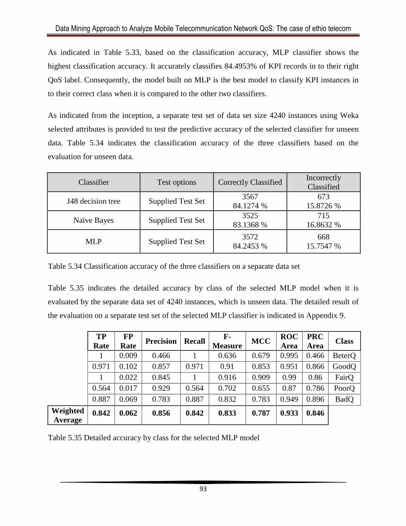
Data Mining Approach to Analyze Mobile Telecommunication Network QoS: The case of ethio telecom
93
As indicated in Table 5.33, based on the classification accuracy, MLP classifier shows the
highest classification accuracy. It accurately classifies 84.4953% of KPI records in to their right
QoS label. Consequently, the model built on MLP is the best model to classify KPI instances in
to their correct class when it is compared to the other two classifiers.
As indicated from the inception, a separate test set of data set size 4240 instances using Weka
selected attributes is provided to test the predictive accuracy of the selected classifier for unseen
data. Table 5.34 indicates the classification accuracy of the three classifiers based on the
evaluation for unseen data.
Classifier Test options Correctly Classified Incorrectly
Classified
J48 decision tree Supplied Test Set 3567
84.1274 %
673
15.8726 %
Naïve Bayes Supplied Test Set 3525
83.1368 %
715
16.8632 %
MLP Supplied Test Set 3572
84.2453 %
668
15.7547 %
Table 5.34 Classification accuracy of the three classifiers on a separate data set
Table 5.35 indicates the detailed accuracy by class of the selected MLP model when it is
evaluated by the separate data set of 4240 instances, which is unseen data. The detailed result of
the evaluation on a separate test set of the selected MLP classifier is indicated in Appendix 9.
TP
Rate
FP
Rate Precision Recall
F-
Measure MCC
ROC
Area
PRC
Area Class
1 0.009 0.466 1 0.636 0.679 0.995 0.466 BeterQ
0.971 0.102 0.857 0.971 0.91 0.853 0.951 0.866 GoodQ
1 0.022 0.845 1 0.916 0.909 0.99 0.86 FairQ
0.564 0.017 0.929 0.564 0.702 0.655 0.87 0.786 PoorQ
0.887 0.069 0.783 0.887 0.832 0.783 0.949 0.896 BadQ
Weighted
Average 0.842 0.062 0.856 0.842 0.833 0.787 0.933 0.846
Table 5.35 Detailed accuracy by class for the selected MLP model
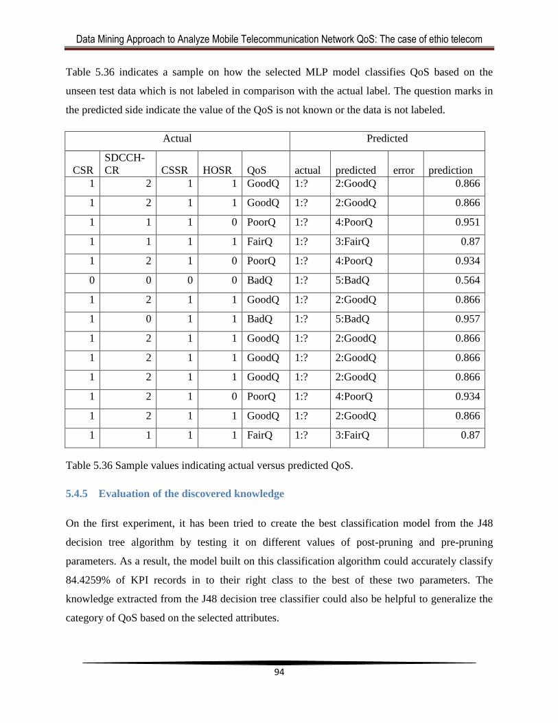
Data Mining Approach to Analyze Mobile Telecommunication Network QoS: The case of ethio telecom
94
Table 5.36 indicates a sample on how the selected MLP model classifies QoS based on the
unseen test data which is not labeled in comparison with the actual label. The question marks in
the predicted side indicate the value of the QoS is not known or the data is not labeled.
Actual Predicted
CSR
SDCCH-
CR CSSR HOSR QoS actual predicted error prediction
1 2 1 1 GoodQ 1:? 2:GoodQ 0.866
1 2 1 1 GoodQ 1:? 2:GoodQ 0.866
1 1 1 0 PoorQ 1:? 4:PoorQ 0.951
1 1 1 1 FairQ 1:? 3:FairQ 0.87
1 2 1 0 PoorQ 1:? 4:PoorQ 0.934
0 0 0 0 BadQ 1:? 5:BadQ 0.564
1 2 1 1 GoodQ 1:? 2:GoodQ 0.866
1 0 1 1 BadQ 1:? 5:BadQ 0.957
1 2 1 1 GoodQ 1:? 2:GoodQ 0.866
1 2 1 1 GoodQ 1:? 2:GoodQ 0.866
1 2 1 1 GoodQ 1:? 2:GoodQ 0.866
1 2 1 0 PoorQ 1:? 4:PoorQ 0.934
1 2 1 1 GoodQ 1:? 2:GoodQ 0.866
1 1 1 1 FairQ 1:? 3:FairQ 0.87
Table 5.36 Sample values indicating actual versus predicted QoS.
5.4.5 Evaluation of the discovered knowledge
On the first experiment, it has been tried to create the best classification model from the J48
decision tree algorithm by testing it on different values of post-pruning and pre-pruning
parameters. As a result, the model built on this classification algorithm could accurately classify
84.4259% of KPI records in to their right class to the best of these two parameters. The
knowledge extracted from the J48 decision tree classifier could also be helpful to generalize the
category of QoS based on the selected attributes.
Data Mining Approach to Analyze Mobile Telecommunication Network QoS: The case of ethio telecom
95
The following rules are important rules taken by traversing through the J48 decision tree
(attached in Appendix 6). The semantics of these rules with the real environment is confirmed by
domain experts.
If CSR=2 and HOSR=2 and CSSR=2 then BeterQ
If CSR=1 and SDCCH_CR=2 and HOSR=1 and CSSR=1 or CSSR=2 then GoodQ
If CSR=1 and SDCCH_CR=2 and HOSR=2 then GoodQ
If CSR=1 and SDCCH_CR=1 and HOSR=1 and CSSR=1 then FairQ
If CSR=1 and SDCCH_CR=1 and HOSR=1 CSSR=1 then FairQ
If CSR=1 and SDCCH_CR=1 and HOSR=0 then PoorQ
If CSR=1 and SDCCH_CR=2 and HOSR=0 then PoorQ
If CSR=1 and SDCCH_CR=1 and HOSR=0 then PoorQ
If CSR=2 and HOSR=0 and 2 then PoorQ
If CSR=0 and HOSR=0 and SDCCH_CR=0 then BadQ
If CSR=1 and SDCCH_CR=0 then BadQ
If CSR=1 and SDCCH_CR=0 then BadQ
The second experiment is conducted on the Naïve Bayes classification algorithm that results the
least classification accuracy of all the experimented classifiers, which is 83.1426 %. It has the
best classification accuracy for KPI instances classified in the 1st ranked cluster or labeled as
‗Better Quality‘, which is 100%.
It takes longer time to build a multilayer perception classification model related to other
classification algorithms in all experiment setups as it has been approved in the third experiment.
Based on the experiments conducted on the MLP classifier on different values of Hidden Layer,
Learning Rate, and Seed value, it has been shown that 84.4953 % classification accuracy can be
achieved to the best of the indicated parameters. This classification accuracy is also the best of
the other two classifiers, J48 decision tree and NaivBayes.
Data Mining Approach to Analyze Mobile Telecommunication Network QoS: The case of ethio telecom
96
Chapter Six
6 Conclusion and Recommendations
6.1 Conclusion
The availability of data by itself do not acquire data mining as a quick fix, it should also be
processed to make it suitable for the data mining task. In this regard, huge amount of data is
generated in every aspect of the industry especially in telecommunications. Once the nature of
the data is understood, it would be easy to call for the corresponding data mining task. In the
context of telecommunications, such tasks include Customer Relationship Management (CRM),
Fraud Detection, and Network Fault detection and isolation which is conducted up on the huge
and complex data generated by the network as this study do.
This study tries to analyze the KPI data indicating the general quality of service (QoS) in a
mobile network by applying different data mining technologies. The cluster model using the k-
means algorithm with its corresponding parameter adjustment provides a worth splitting clusters
based on the natural proximity of the KPI data, discretized as ‗0‘or ‗1‘ or ‗2‘, related to the
concept hierarchy. On the other hand, various experiments are conducted to identify the best
classification model. Thus, the classification model built on MLP has the best accuracy relative
to the J48 and the Naïve Bayes classification algorithm.
Among the KPIs studied, Call Success Rate (CSR) could measure an end to end performance of
a mobile network since CSR indicates the success of a call from its initiation when Standalone
Dedicated Control Channel (SDCCH) is allocated to establish a call; Traffic Channel (TCH) is
assigned to hold the call until it comes to a deliberate termination which otherwise could be a
dropped call. On the other hand the SDCCH and TCH KPIs decide the performance of the Call
Setup Success Rate (CSSR) KPI since to set up a call both call establishment and call persistency
resources are mandatory. Thus, the two logical channels, SDCCH and TCH, are crucial for the
QoS experienced by the customer.
The clustering model built on the simple k-means algorithm provides a better understanding of
the KPI data as it cluster the instances based on their natural proximity. Moreover, the
Data Mining Approach to Analyze Mobile Telecommunication Network QoS: The case of ethio telecom
97
interpretation is very close to the real mobile network optimization knowledge of the domain
experts. So that it is a suitable model to study the real nature and concurrency of the mobile
network general QoS KPIs.
The multilayer perception classification model, which is an implementation of neural network, is
the best model in classifying the KPIs to their ranked cluster labeled as ‗Better Quality‘, ‗Good
Quality‘, ‗Fair Quality‘, ‗Poor Quality‘ and ‗Bad Quality‘.
The rules taken by traversing through the J48 decision tree are important rules that could be used
to generalize the network quality of service in the real situation.
Effective analysis of GSM networks is currently challenging because of large volume of data
collected from network elements and evolution towards better technologies might further
increase the size and complexity of data. It is essential to apply data mining to extract the
relevant information to a level which can be easily managed.
Finally, as there is no cut and dried data set available for a data mining task, different challenges
are faced from data preprocessing through data transformation up to the data mining task. First of
all, there is no split point between the threshold (t) and the ideal (maximum desirable) values for
each KPI. Secondly, the data set taken from the network management system is not labeled. It
needs a considerable time and strategy to do this task. And lastly, the large data set provided for
the data mining task not only needs a considerable computational resource but also challenges
the efficiency of the algorithm. Most of the challenges are vanquished by this research which can
be considered as strength.
Data Mining Approach to Analyze Mobile Telecommunication Network QoS: The case of ethio telecom
98
6.2 Recommendation
Based on the findings, the following recommendations are presented:
The data mining tasks performed on this specific study revolves around clustering and
classification. The cluster model experiment is undertaken based on the simple k-means
algorithm, where the best cluster model selection is on the basis of parameter adjustment.
On the other hand, the Multilayer Perception classification model is selected relative to
J48 and Naïve Bayes classification algorithms. However, other clustering and
classification algorithms might reveal even a better accuracy.
Even though the research is done for academic achievements, the output can be used for a
better understanding of different KPIs and their relationship as well as to generalize
network quality of service based on important rules. These can be applied in the mobile
network optimization task.
The concept of QoS is not only a big issue in a second generation (2G) network, but also
it is the main concern of the third generation (3G), as well as the fourth generation (4G)
network. Moreover, this study is concerned about the general quality of service KPIs in
the mobile telecommunication network; there are also other KPIs that are specifically
designed to measure the service quality of data, internet, and others. These might leave a
room to conduct further studies

Data Mining Approach to Analyze Mobile Telecommunication Network QoS: The case of ethio telecom
99
References
Ali, M. Shehzad, A., & Akram, M. (2010). Radio Access Network Audit & Optimization in GSM
(Radio Access Network Quality Improvement Techniques). International Journal of
Engineering & Technology IJET-IJENS Vol: 10 No: 01
Almeida, L. (1997). Handbook of Neural Computation release. IOP Publishing Ltd and Oxford
University Press
Breiman, L., Friedman, J., Olshen, R., Stone, C. (1984). Classification and Regression Trees.
Wadsworth International Group.
Bouckaert, R., Frank, E., Hall, M., Kirkby, R., Reutemann, P., Seewald, A., Scuse, D. (2014). Weka
(Version 3-7-11) [Computer software]. University of Waikato: Hamilton.
Carvalho, F. & Magedanz, T. (2007). Telecommunication Systems and Technologies. Berline:
Encyclopedia of Life Support System (ELSS)
Chandra, P. (2005). Bulletproof wireless security: GSM, UMTS, 802.11 and Ad Hoc Security.
Elsevier Inc.
Chapman, P. (2000). CRISP-DM 1.0: Step-by-step data mining guide. SPSS Inc.
Cios, K., Pedrycz, W., Swiniarski, R., Kurgan, L. (2007). Data mining: A knowledge discovery
approach. Springer Science & Business Media, LLC
Clemm, A. (2007). Network management fundamentals. Cisco Systems, Inc.
Dunlop, J. & Smith, D, (2000). Telecommunications engineering, Third edition. Chapman & Hall
Esling, P. & Agon, C. (2012). Time-Series Data Mining. ACM Comput. Surv. 45(1), Article 12
ethio-telecom (2012). Company profile.
ethio-telecom (November 2013). Press release. Retrieved from
http://www.ethiotelecom.et/news/news.php?id=88

Data Mining Approach to Analyze Mobile Telecommunication Network QoS: The case of ethio telecom
100
ethio-telecom (September 2011). Press release. Retrieved from
http://www.ethiotelecom.et/press/news.php?id=37
ethio-telecom (September 2012). Press release. Retrieved from
http://www.ethiotelecom.et/press/news.php?id=74
ETSI (2004). Speech Processing, Transmission and Quality Aspects (STQ); QoS aspects for popular
services in GSM and 3G networks; Part 6: Post processing and statistical methods.
Technical Specification, TS, 102 250-6 V1.2.1
ETSI (2010). Key Performance Indicators (KPI) for UMTS and GSM. Technical Specification,
3GPP TS 32.410 version 9.0.0 Release 9.
Fayyad, U., Piatetsky, G., & Smyth, P. (1996b). From Data Mining to Knowledge Discovery in
Databases. American Association for Artificial Intelligence.
Fayyad, U., Piatetsky, G., & Smyth, P. (1996c). Mining Scientific Data. Communications of the
ACM, 39(11),pp. 51-57
Fong, S. (2011). Data Mining for Resource Planning and QoS Supports in GSM Networks. Journal
of Emerging Technologies in Web Intelligence, Vol. 3, No. 2.
Gebremeskal, G. (2006). Data Mining Application in Supporting Fraud Detection on Ethio-Mobile
Services. (Masters Thesis, Addis Ababa University)
Gómez, G & Sánchez, R (eds), (2005). End-to-End Quality of Service over Cellular Networks. John
Wiley & Sons Ltd
Gorunescu, F. (2011). Data Mining: Concepts, Models and Techniques. Springer
Haider, B., Zafrullah, M. & Islam, M. K. (2009). Radio Frequency Optimization & QoS Evaluation in
Operational GSM Network. Proceedings of the World Congress on Engineering and
Computer Science, Vol I.

Data Mining Approach to Analyze Mobile Telecommunication Network QoS: The case of ethio telecom
101
Halonen, T. Romero, J. & Melero, J. (eds.), (2003). GSM, GPRS and EDGE Performance: evolution
towards 3G/UMTS, Second edition. John Wiley & Sons Ltd.
Han, J. & Kamber, M. (2006). Data Mining: Concepts and Techniques, Second Edition. Elsevier
Inc.
Hardy, C. (2001). QoS: Measurement and evaluation of telecommunications quality of service.
Chichester: John Wiley & Sons
Harrington, P. (2012). Machine learning in action. Manning Publications
Horak, R. (2007), Telecommunications and data communications handbook. John Wiley & Sons
ITU (2013). World Telecommunication/ICT Indicators database. Retrieved from
http://www.itu.int/en/ITU-D/Statistics/Pages/stat/default.aspx
ITU-CCITT (2007). Quality of service and dependability vocabulary, Series E: Overall network
operation, Telephone service, Service operation and human factors, Geneva: ITU
ITU-T (2000). TMN Management Functions, Series M: TMN and Network Maintenance:
International Transmission Systems Telephone Circuits, Telegraphy, Facsimile, And Leased
Circuits. M.3400 Recommendation
Joseph, M. (2013). Data Mining and Business Intelligence Applications in Telecommunication
Industry. International Journal of Engineering and Advanced Technology (IJEAT), pp 2249
– 8958, Volume-2, Issue-3
Kamber, M., Pei, J., & Han, J. (2011). Data mining: Concepts and techniques, Third Edition.
Elsevier Inc.
Krose, V. & Smagt, P. (1996). An Introduction to neural network. The University of Amesterdam

Data Mining Approach to Analyze Mobile Telecommunication Network QoS: The case of ethio telecom
102
Kumar, P., Anuradha, B., Naresh, V. (2004). Improvement Of Key Performance Indicators and QoS
Evaluation in Operational GSM Network. International Journal of Engineering Research
and Applications (IJERA), Vol. 1, Issue 3, pp.411-417.
Kumar, V., Tan, P., & Steinbach (2001), Introduction to Data Mining. CRC Press
Kumar, V., Tan, P., & Steinbach, M. (2001). Introduction to data mining. CRC Press, LLC
Kyriazakos, S. & Karetsos, G. (2004). Practical radio resource management in wireless systems.
Artech House
Kyriazakos, S., Papaoulakis, N., Nikitopoulos, D., Gkroustiotis, E., Kechagias, C., Karambalis, C.,
& Karetsos, G. (2002). A Comprehensive Study and Performance Evaluation of Operational
GSM and GPRS Systems under Varying Traffic Conditions. IST Mobile and Wireless
telecommunications Summit, 2002, Greece
Laiho, J., Wacker, A. & Novosad, T. (eds.), (2006). Radio network planning and optimization for
UMTS, Second Edition. John Wiley & Sons Ltd
Lehtim aki, P. (2008). Data analysis methods for cellular network performance optimization.
(Docteral dissertation, Helsinki University of Technology).
Lempiäinen, J. and Manninen, M. (2002). Radio interface system planning for GSM/GPRS/UMTS.
Kluwer Academic Publishers
Maimon, O. and Rokach, L.(eds.) (2010). Data Mining and Knowledge Discovery Handbook.
Second Edition. Springer
Mariscal, G., Marba, O. & Fernandez, C. (2010). A Survey of Data Mining And Knowledge
Discovery Process Models And Methodologies. The Knowledge Engineering Review, Vol.
25:2, pp.137–166.

Data Mining Approach to Analyze Mobile Telecommunication Network QoS: The case of ethio telecom
103
Melaku, G. (2009). Applicability of Data Mining Techniques to Customer Relationship Management
(CRM): The Case of Ethiopian Telecommunication Corporation's (ETC) Code Division
Multiple Access (CDMA) Telephone Service. (Masters thesis, Addis Ababa University)
Mishra, A. (2004). Fundamentals of cellular network planning and optimization: 2G/2.5G/3G...
evolution to 4G. John Wiley & Sons, Ltd
Multanen M., Kimmo Raivio, K., & Lehtim, P. (2006). Hierarchical Analysis of GSM Network
Performance Data. Helsinki University of Technology.
Nadaf, M. & Kadam, V. (2013). Data Mining in Telecommunication.Volume-2, Issue-3, pp 2319 –
2526
Pitas, C. Chourdaki, K. Panagopoulos, A & Constantinou, P. (2011). QoS Mining Methods for
Performance Estimation of Mobile Radio Networks. 10th Int’l Conf. on Measurement of
Speech, Audio and Video Quality in Networks (MESAQIN). Athens: National Technical
University
Popoola, J. J., Megbowon, I. O., & Adeloye, V. S. A. (2009). Performance Evaluation and Improvement
on Quality of Service of Global System for Mobile Communications in Nigeria. Journal of
Information Technology Impact, Vol. 9, No. 2, pp. 91-106
Pressman, R. (2005). Software Engineering: A Practitioner’s Approach, 6th edition, McGraw-Hill
Rahnema M., (2008). UMTS Network planning, optimization, and inter-operation with GSM. John
Wiley & Sons
Rokach, L. & Maimon, O. (2008). Data mining with decision trees: Theory and Applications. World
Scientific Publishing Co. Pte. Ltd.
Singh Y. & Chauhan S. (2009). Neural Networks in Data Mining. Journal of Theoretical and
Applied Information Technology. Retreived from: www.jatit.org

Data Mining Approach to Analyze Mobile Telecommunication Network QoS: The case of ethio telecom
104
Sorokosz, L. & Zieniutycz, W. (2012). Artificial Neural Networks in Microwave Components and
Circuits Modeling. Przeglad Elektrotechniczny (Electrical Review)
Sumathi, S. & Sivanandam S. (2006). Introduction to Data Mining and its Applications. Springer
Tele Management Forum (2000). Telecom Operations Map. GB910
The Federal Democratic Republic of Ethiopia (2011). Federal Negarit Gazeta, 17th
, Year No. 11,
Addis Ababa 28th January
Tyrrell, S. (2000). The many dimensions of the software processes. ACM Crossroads 6(4), pp. 22–
26.
Vehviläinen, V. (2004). Data mining for managing intrinsic quality of service in digital mobile
telecommunications networks. (Doctoral thesis, Tampere University of Technology).
Ville, B. (2006). Decision trees for business intelligence and data mining: Using SAS enterprise
miner. Cary, NC: SAS Institute Inc.
Weiss, G. (2009). Data Mining in the Telecommunications Industry. USA: Global Fordham
University.
Williams, G (2011). Data mining with rattle and R: The art of excavating data for knowledge
discovery. Springer
Witten, I, Frank, E., and Hall, M. (2011). Data Mining Practical Machine Learning Tools and
Techniques, Third Editio. , Morgan Kaufmann Publishers
Wu, X., Kumaret, V., Quinlanal, J. R., Ghosh, J., Yang, Q., & Motoda, H. (2007). Top 10 algorithms
in data mining. London: Springer
Yang, Q. & Wu, X. (2006). 10 Challenging Problems in Data Mining Research. International
Journal of Information Technology & Decision Making Vol. 5, No. 4, pp. 597–604, World
Scientific Publishing Company

Data Mining Approach to Analyze Mobile Telecommunication Network QoS: The case of ethio telecom
105
Ye, N. (ed.), (2003). The handbook of data mining. Lawrence Erlbaum Associates, Inc.
Yeshinegus, G. (2013). Predictive Modeling for Fraud Detection in Telecommunications: The Case
of Ethio-Telecom. AAU, (Masters thesis, Addis Ababa University)
Zaki, M. & Meira, J. W. (2013). Data Mining and Analysis: Fundamental Concepts and Algorithms.
Cambridge University Press
Zhang, Q. & Gupta, K. (2000). Neural Network for RF and Microwave Design. Artech House
Publisher.
Zhao, Y. & Zhang, Y. (2007). Comparison of decision tree methods for finding active objects.
Bejing: National Astronomical Observatories.
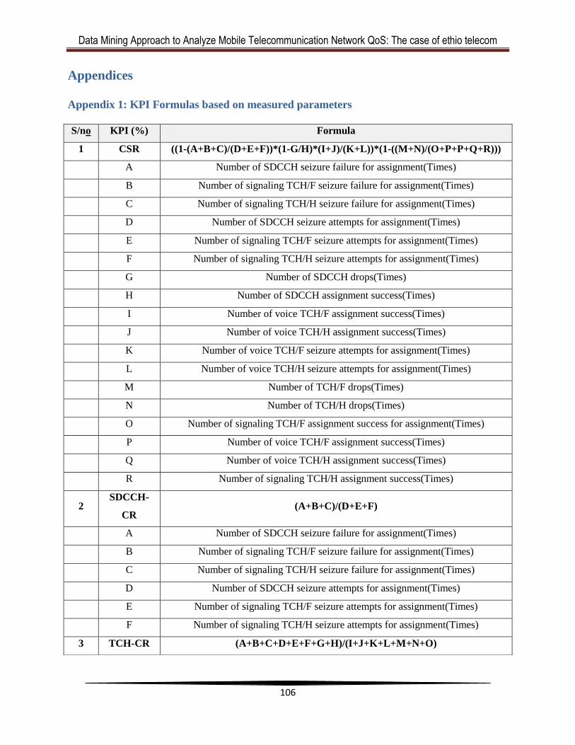
Data Mining Approach to Analyze Mobile Telecommunication Network QoS: The case of ethio telecom
106
Appendices
Appendix 1: KPI Formulas based on measured parameters
S/no KPI (%) Formula
1 CSR ((1-(A+B+C)/(D+E+F))*(1-G/H)*(I+J)/(K+L))*(1-((M+N)/(O+P+P+Q+R)))
A Number of SDCCH seizure failure for assignment(Times)
B Number of signaling TCH/F seizure failure for assignment(Times)
C Number of signaling TCH/H seizure failure for assignment(Times)
D Number of SDCCH seizure attempts for assignment(Times)
E Number of signaling TCH/F seizure attempts for assignment(Times)
F Number of signaling TCH/H seizure attempts for assignment(Times)
G Number of SDCCH drops(Times)
H Number of SDCCH assignment success(Times)
I Number of voice TCH/F assignment success(Times)
J Number of voice TCH/H assignment success(Times)
K Number of voice TCH/F seizure attempts for assignment(Times)
L Number of voice TCH/H seizure attempts for assignment(Times)
M Number of TCH/F drops(Times)
N Number of TCH/H drops(Times)
O Number of signaling TCH/F assignment success for assignment(Times)
P Number of voice TCH/F assignment success(Times)
Q Number of voice TCH/H assignment success(Times)
R Number of signaling TCH/H assignment success(Times)
2 SDCCH-
CR (A+B+C)/(D+E+F)
A Number of SDCCH seizure failure for assignment(Times)
B Number of signaling TCH/F seizure failure for assignment(Times)
C Number of signaling TCH/H seizure failure for assignment(Times)
D Number of SDCCH seizure attempts for assignment(Times)
E Number of signaling TCH/F seizure attempts for assignment(Times)
F Number of signaling TCH/H seizure attempts for assignment(Times)
3 TCH-CR (A+B+C+D+E+F+G+H)/(I+J+K+L+M+N+O)

Data Mining Approach to Analyze Mobile Telecommunication Network QoS: The case of ethio telecom
107
A Number of voice TCH/F seizure failure for assignment(Times)
B Number of data TCH/F seizure failure for assignment(Times)
C Number of voice TCH/H seizure failure for assignment(Times)
D Number of data TCH/H seizure failure for assignment(Times)
E Number of voice TCH/F seizure failure for handover(Times)
F Number of data TCH/F seizure failure for handover(Times)
G Number of voice TCH/H seizure failure for handover(Times)
H Number of data TCH/H seizure failure for handover(Times)
I Number of voice TCH/F seizure attempts for assignment(Times)
J Number of data TCH/F seizure attempts for assignment(Times)
K Number of voice TCH/H seizure attempts for assignment(Times)
L Number of data TCH/H seizure attempts for assignment(Times)
M Number of voice TCH/F seizure attempts for handover(Times)
N Number of data TCH/F seizure attempts for handover(Times)
O Number of voice TCH/H seizure attempts for handover(Times)
P Number of data TCH/H seizure attempts for handover(Times)
4 DCR (A+B)/(C+D+E+F)
A Number of TCH/F drops(Times)
B Number of TCH/H drops(Times)
C Number of signaling TCH/F assignment success for assignment(Times)
D Number of voice TCH/F assignment success(Times)
E Number of voice TCH/H assignment success(Times)
F Number of signaling TCH/H assignment success(Times)
5 SDCCH-
CDR A/(B+C+D)
A Number of SDCCH drops(Times)
B Number of SDCCH seizure attempts for assignment(Times)
C Number of signaling TCH/F seizure attempts for assignment(Times)
D Number of signaling TCH/H seizure attempts for assignment(Times)
6 TCH-CDR (A+B)/(C+D+E+F+G+H+I)
A Number of TCH/F drops(Times)
B Number of TCH/H drops(Times)
C Number of voice TCH/F assignment success(Times)
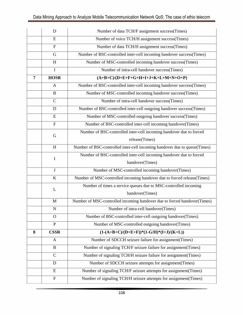
Data Mining Approach to Analyze Mobile Telecommunication Network QoS: The case of ethio telecom
108
D Number of data TCH/F assignment success(Times)
E Number of voice TCH/H assignment success(Times)
F Number of data TCH/H assignment success(Times)
G Number of BSC-controlled inter-cell incoming handover success(Times)
H Number of MSC-controlled incoming handover success(Times)
I Number of intra-cell handover success(Times)
7 HOSR (A+B+C)/(D+E+F+G+H+I+J+K+L+M+N+O+P)
A Number of BSC-controlled inter-cell incoming handover success(Times)
B Number of MSC-controlled incoming handover success(Times)
C Number of intra-cell handover success(Times)
D Number of BSC-controlled inter-cell outgoing handover success(Times)
E Number of MSC-controlled outgoing handover success(Times)
F Number of BSC-controlled inter-cell incoming handover(Times)
G
Number of BSC-controlled inter-cell incoming handover due to forced
release(Times)
H Number of BSC-controlled inter-cell incoming handover due to queue(Times)
I
Number of BSC-controlled inter-cell incoming handover due to forced
handover(Times)
J Number of MSC-controlled incoming handover(Times)
K Number of MSC-controlled incoming handover due to forced release(Times)
L
Number of times a service queues due to MSC-controlled incoming
handover(Times)
M Number of MSC-controlled incoming handover due to forced handover(Times)
N Number of intra-cell handover(Times)
O Number of BSC-controlled inter-cell outgoing handover(Times)
P Number of MSC-controlled outgoing handover(Times)
8 CSSR (1-(A+B+C)/(D+E+F))*(1-G/H)*(I+J)/(K+L))
A Number of SDCCH seizure failure for assignment(Times)
B Number of signaling TCH/F seizure failure for assignment(Times)
C Number of signaling TCH/H seizure failure for assignment(Times)
D Number of SDCCH seizure attempts for assignment(Times)
E Number of signaling TCH/F seizure attempts for assignment(Times)
F Number of signaling TCH/H seizure attempts for assignment(Times)
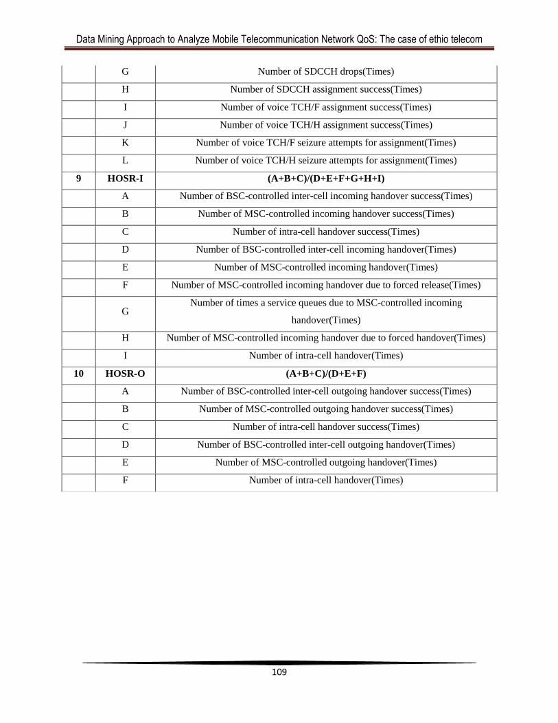
Data Mining Approach to Analyze Mobile Telecommunication Network QoS: The case of ethio telecom
109
G Number of SDCCH drops(Times)
H Number of SDCCH assignment success(Times)
I Number of voice TCH/F assignment success(Times)
J Number of voice TCH/H assignment success(Times)
K Number of voice TCH/F seizure attempts for assignment(Times)
L Number of voice TCH/H seizure attempts for assignment(Times)
9 HOSR-I (A+B+C)/(D+E+F+G+H+I)
A Number of BSC-controlled inter-cell incoming handover success(Times)
B Number of MSC-controlled incoming handover success(Times)
C Number of intra-cell handover success(Times)
D Number of BSC-controlled inter-cell incoming handover(Times)
E Number of MSC-controlled incoming handover(Times)
F Number of MSC-controlled incoming handover due to forced release(Times)
G
Number of times a service queues due to MSC-controlled incoming
handover(Times)
H Number of MSC-controlled incoming handover due to forced handover(Times)
I Number of intra-cell handover(Times)
10 HOSR-O (A+B+C)/(D+E+F)
A Number of BSC-controlled inter-cell outgoing handover success(Times)
B Number of MSC-controlled outgoing handover success(Times)
C Number of intra-cell handover success(Times)
D Number of BSC-controlled inter-cell outgoing handover(Times)
E Number of MSC-controlled outgoing handover(Times)
F Number of intra-cell handover(Times)
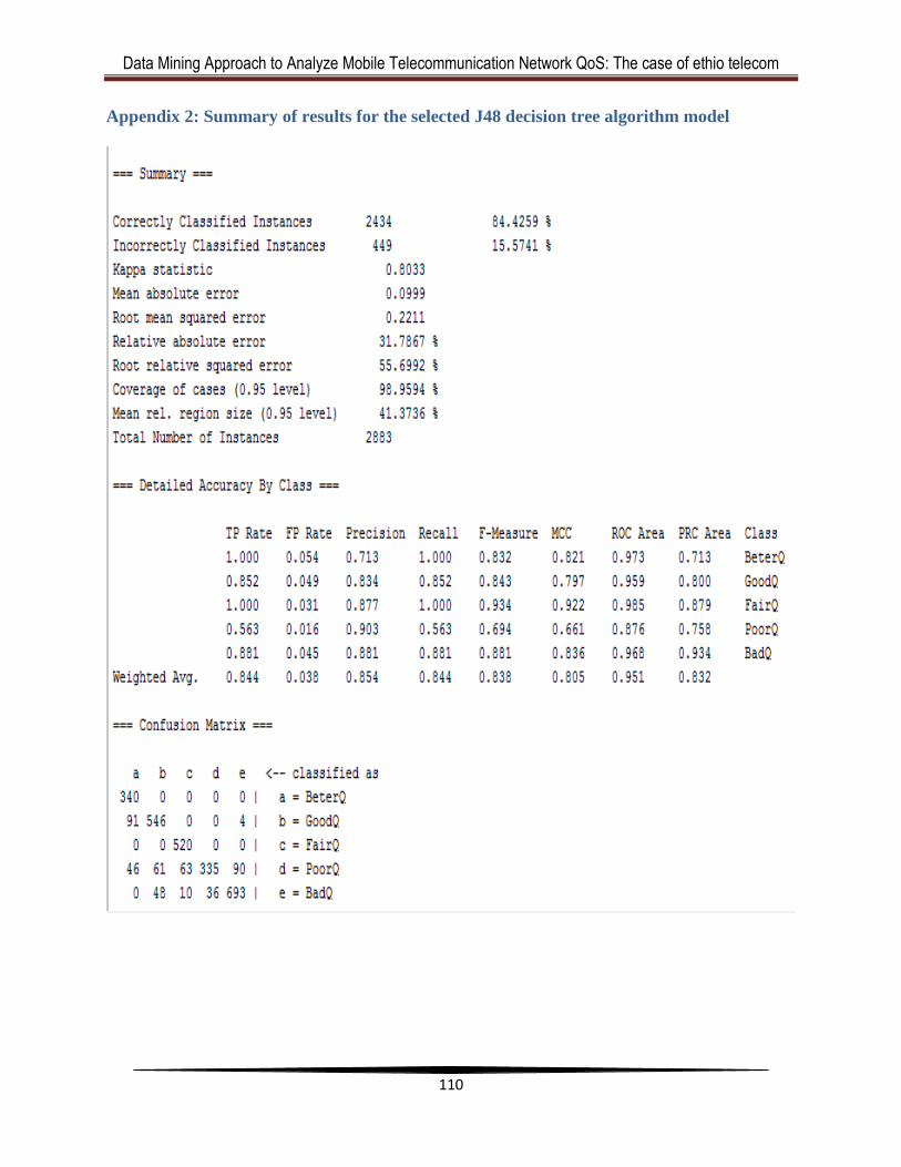
Data Mining Approach to Analyze Mobile Telecommunication Network QoS: The case of ethio telecom
110
Appendix 2: Summary of results for the selected J48 decision tree algorithm model
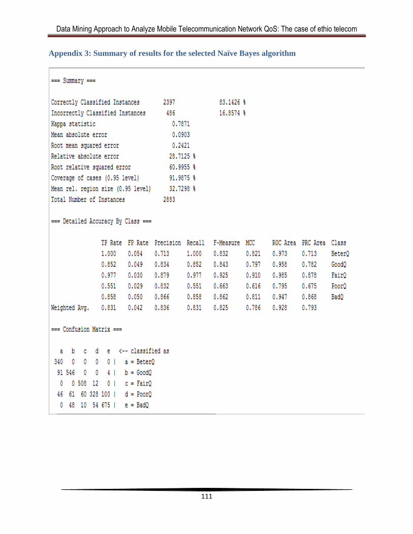
Data Mining Approach to Analyze Mobile Telecommunication Network QoS: The case of ethio telecom
111
Appendix 3: Summary of results for the selected Naïve Bayes algorithm
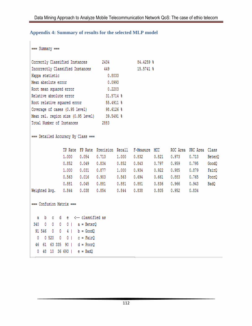
Data Mining Approach to Analyze Mobile Telecommunication Network QoS: The case of ethio telecom
112
Appendix 4: Summary of results for the selected MLP model
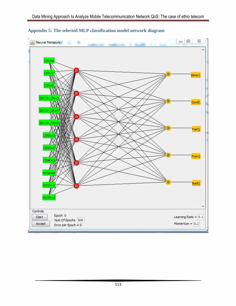
Data Mining Approach to Analyze Mobile Telecommunication Network QoS: The case of ethio telecom
113
Appendix 5: The selected MLP classification model network diagram
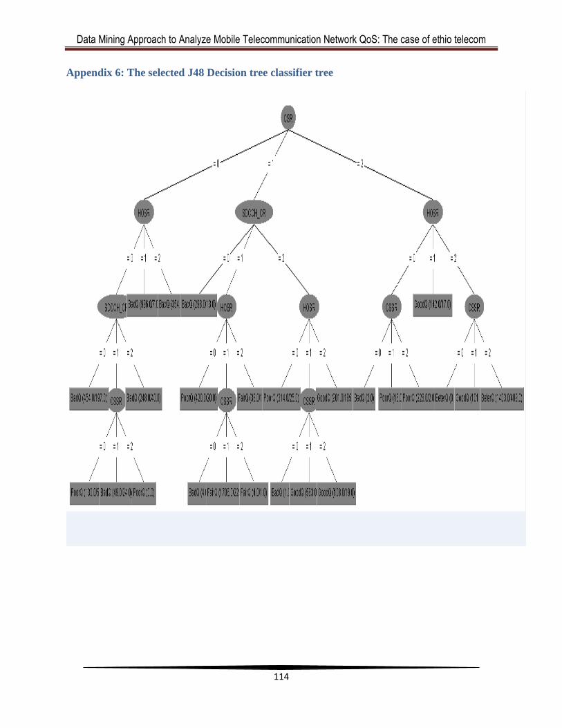
Data Mining Approach to Analyze Mobile Telecommunication Network QoS: The case of ethio telecom
114
Appendix 6: The selected J48 Decision tree classifier tree
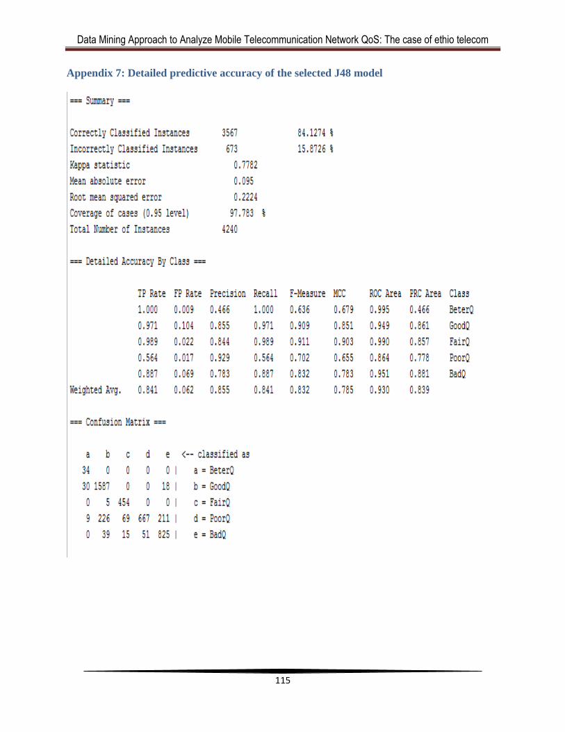
Data Mining Approach to Analyze Mobile Telecommunication Network QoS: The case of ethio telecom
115
Appendix 7: Detailed predictive accuracy of the selected J48 model
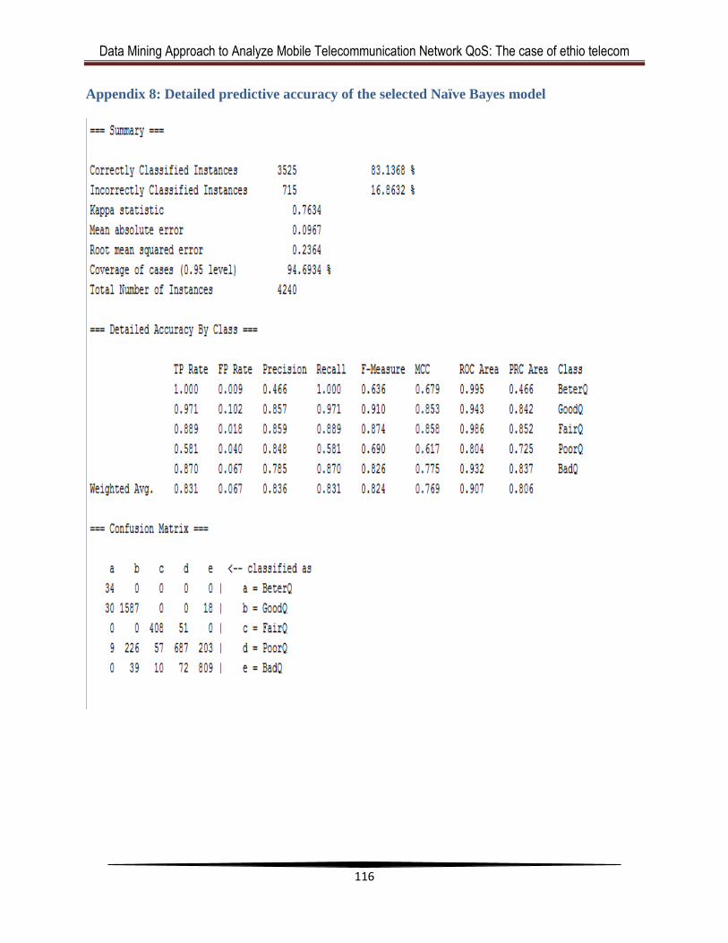
Data Mining Approach to Analyze Mobile Telecommunication Network QoS: The case of ethio telecom
116
Appendix 8: Detailed predictive accuracy of the selected Naïve Bayes model
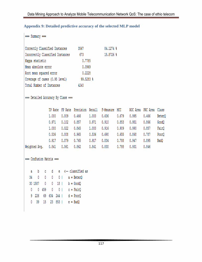
Data Mining Approach to Analyze Mobile Telecommunication Network QoS: The case of ethio telecom
117
Appendix 9: Detailed predictive accuracy of the selected MLP model

Data Mining Approach to Analyze Mobile Telecommunication Network QoS: The case of ethio telecom
118
DECLARATION
I declare that the thesis is my original work and has not been presented for a degree in any other
university.
-------------------------- -----------------------
Signature Date
This thesis has been submitted for examination with my approval as university advisor.
---------------------------------
Ato Getachew Jemaneh