A Framework for Optimization of Sensor Activationusing Most Permissive Observers

Eric DallalUniversity of MichiganDepartment of EECSedallal@umich.edu

Stephane LafortuneUniversity of MichiganDepartment of EECS

stephane@eecs.umich.edu

Abstract—This paper considers the problem of finding dy-namic sensor activation policies that satisfy the property of K-diagnosability for discrete event systems modeled by finite stateautomata. We begin by choosing a suitable information state forthe problem and defining a controller. We then define a structurecalled the most permissive observer, which provides all feasiblesolutions for the controller (i.e., for sensor activations). By formu-lating the problem as a state disambiguation problem, we prove anumber of monotonicity properties about the information state.Finally, we show that this formulation allows us to efficientlycompute the set of all satisfactory control decisions at all pointsin the system’s execution.

I. INTRODUCTION

This paper studies problems of dynamic sensor optimizationin discrete event systems. Our model assumes that a systemis modeled as a deterministic finite state automaton and thatwe have sensors that can detect the occurrence of only asubset of events. These events are classified as “monitorable”and we may choose not to observe them. In engineeringproblems, this might be useful in order to save energy in thesensors if these are costly to operate. Alternatively, there maybe high energy requirements involved in communicating thesensor measurements. Another possibility is that we wouldlike to minimize communication of sensor measurements forthe purpose of maintaining security. For any of these or otherreasons, we assume that we would like to minimize sensoractivations (for a more detailed explanation of the motivationfor dynamic sensor activation, see [1]. For a concrete example,see [2]). Additionally, we assume that, among the remaininginherently unobservable events, there is a significant eventwhose occurrence we would like to be able to determine. Inthis work, we consider the event in question to be a fault event.The control problem is to determine which sensors to turnon/off at every point in time while maintaining the property ofK-diagnosability. The K-diagnosability property is similar tothat of diagnosability as found in [3], but where the diagnosismust be made with a delay of at most K events. Specifically,the system must always be able to distinguish between faultyand non-faulty executions within K + 1 events after a fault.

A number of other recent works have considered theproblem of optimizing sensor activations while maintainingsome notion of diagnosability; see, e.g., [1], [4], [5]. In [4],dynamic programming is used to find an optimal solution tothe problem of optimizing sensor activations while maintaining

the property of diagnosability simultaneously for automatawith multiple fault types. In [5], game theory is used first todefine a structure called most permissive observer (which willbe redefined in this paper). Results from the theory of gameson graphs are then used, resulting in algorithms that solvethe optimal sensor activation problem. Their methodology isextended to opacity in [6]. In [1], the problem of decentralized,or multi-agent, diagnosis is solved through a “window-basedpartition” approach. Algorithms that run in time polynomialin the window partition size are given for both the centralizedand decentralized event diagnoses cases.

Several criteria can be used for guiding the solution of thedynamic sensor activation problem. A simple one is that ofstate disambiguation: sensors must be activated often enoughso that certain pairs of discrete states should never be confusedat run-time, along any system trajectory. State disambiguationrequirements arise naturally at the discrete-event level. Forexample, the discrete-event-theoretic property of observabil-ity [7], which is part of the necessary and sufficient conditionsfor the existence of discrete-event controllers for partially-observed systems, can be expressed as a state disambiguationproperty (cf. [8]). We demonstrate in this paper that K-diagnosability can be mapped to a problem of state disam-biguation over a suitable refinement of the discrete state space.Hence, our results can be adapted, with simple modifications,to solve a standard state disambiguation problem.

Our work is most closely related to the approach of [5], inthat the goal is maintaining the K-diagnosability property fora system modeled by an automaton, and that we both definethe “most permissive observer” (MPO), a discrete structurethat captures all controllers that constitute feasible solutions.In [5], the MPO is defined through game theory and the theoryof games on graphs. Our MPO is defined as a bipartite graphover suitable information states. Although we both end upwith the same structure, our goal is to develop an informationstate based approach to the construction of the MPO, whichallows for two benefits: first, a clearer understanding of infor-mational properties of the MPO; second, a greater adaptabilityin being applied to other dynamic optimization problems indiscrete event systems. As in [5], we tackle the dynamiccontrol problem in two parts: first, we construct the MPOwhich contains all controllers that satisfy the K-diagnosabilityproperty; second, we use the MPO as a “feasbile space” over

2011 50th IEEE Conference on Decision and Control andEuropean Control Conference (CDC-ECC)Orlando, FL, USA, December 12-15, 2011

978-1-61284-799-3/11/$26.00 ©2011 IEEE 2711

which to optimize. This work addresses the first part. With theMPO, we can then use techniques from [5] or [4] to find asingle optimal solution.

Our notion of MPO was first introduced in [9]. In [9], weproved that our information state was “sufficient” in the sensethat no generality is lost by examining only controllers basedon that information state. Section II of this paper will recallsome definitions from [9]. In the main body of this paper, weshow how to map the K-diagnosability problem to the statedisambiguation problem. The most significant contribution ofthis paper is that this approach allows us to establish theexistence of a simple and efficient test on the informationstate for determining whether or not any particular controldecision maintains the K-diagnosability property. We alsocharacterize informational properties of the MPO and thenpresent an efficient algorithm for its construction.

For some references on other concepts of observers inlogical discrete-event models, see [10]–[13].

The rest of this paper is organized as follows. SectionII describes the model under consideration, followed by anumber of definitions related to our information state. SectionIII formally defines the K-diagnosability property, explainshow to formulate it as a state disambiguation problem, anddefines the recursive structure of the MPO. Section IV estab-lishes a number of theorems that show how the “extendedspecification” (from the literature on state disambiguation,see [14]) can be used to efficiently compute the MPO on-line. Finally, we have conclusions and references. Note thatall proofs have been omitted due to space constraints.

II. AUGMENTED STATES AND THE INFORMATION STATE

Consider a deterministic automaton G = (X,E, f, x0),where X is the set of states, E is the set of events, f :X × E → X is the system’s partial transition function, andx0 is the initial state. Define L(G) to be the language of G,that is, the set of all strings of events that can occur in G.Assume that the set E is partitioned into four disjoint setsE = Eo ∪ Es ∪ Euo ∪ Ef , each corresponding to differentcategories of events: Eo is the set of events that are alwaysmonitored, Es is the set of events that are observable but maynot always be monitored (for example, if a sensor is turnedoff), Ef is the set of unobservable faulty events (or any setof important unobservable events whose occurrence we wouldlike to diagnose) and Euo is the set of unobservable (non-faulty) events. In this work, we assume that there is only onefault event.

We wish to dynamically diagnose any occurrence of the faultevent. Here, we use the notion of K-diagnosability (formallydefined in section III), which states that we must be able todiagnose the occurrence of any fault (with certainty) withinat most K + 1 events after the fault event. At each pointin the system’s execution, we wish to find the set of allcontrol decisions that allow the system to maintain the K-diagnosability property, after each run of control decisions andobserved events. The MPO, which we will define in section

III and show how to construct in section IV, contains allcontrollers that constitute feasible solutions to this problem.

The remainder of this section briefly provides the mathemat-ical preliminaries necessary for defining the MPO as it pertainsto the problem of K-Diagnosability. Parts of this section arerecalled or modified from [9], where we first introduced ourMPO.

Definition II.1 (Augmented State). The augmented state isa pair (x, n) ∈ X × {−1, 0, 1, . . .}, where, n represents a“count” of the number of events (of all kinds) that haveoccurred since a fault event occurred, or −1 if no faultevent has occurred. The set of such states is denoted byX+ = X × {−1, 0, 1, . . .}. The initial augmented state isx+

0 = (x0,−1). For any augmented state x+ ∈ X+, let thestate and count components be denoted by S(x+) and N(x+),respectively, so that x+ = (S(x+), N(x+)).

Definition II.2 (Augmented Transition Function). We nextdefine the augmented transition function g : X+ ×E → 2X

+

on augmented states that is induced by the automaton G =(X,E, f, x0) and the partition of event set E. Formally, forany u = (xu, nu) and event e, we have:• Case 1: If nu = −1 and e /∈ Ef then g(u, e) ={(f(xu, e),−1)}.

• Case 2: If nu = −1 and e ∈ Ef then g(u, e) ={(f(xu, e), 0)}.

• Case 3: If nu ≥ 0 and e /∈ Ef then g(u, e) ={(f(xu, e), nu + 1)}.

• Case 4: If nu ≥ 0 and e ∈ Ef then g(u, e) ={(f(xu, e), 0), (f(xu, e), nu + 1)}.

It is because of this last case that g is defined as a mappingfrom augmented states to sets of augmented states rather thansimply to augmented states. So that the function can be appliediteratively, we define g applied to a set as the union of gapplied to each augmented state in the set. Mathematically,we write: g(U, e) =

⋃u∈U g(u, e). This definition is extended

to strings (rather than merely events) in the usual way. Finally,we define g(s) = g(x+

0 , s) for brevity.

Definition II.3 (Augmented Automaton). We define the aug-mented automaton as the automaton G+ = (X+, E, g, x+

0 )defined over augmented states that is induced from the originalautomaton G. Specifically, we take X+ and x+

0 as defined inDefintion II.1 and g as defined in Definition II.2 (the event setE remains the same). Note that G+ might not be deterministic,even if G is, due to case 4 in the definition of the augmentedstate transition function g. Furthermore, without a bound onthe count component of augmented states, G+ might not befinite in size (in section IV, we will use a trimmed version ofG+ that avoids this problem).

Definition II.4 (Run). A run ρ of length n is defined asa sequence C0, e0, . . . , Cn−1, en−1 of control decisions orsensor activations (the Ci’s, which are subsets of events tomonitor) and observed events (the ei’s). Since the events areobserved, they must be among the monitored events. That is,ei ∈ Ci, for all i = 0, . . . , n− 1. On the other hand, the strict

2712

alternation of control decisions and observed events reflectsthe assumption that control decisions are only changed uponthe observance of an event. Denote by Rn the set of runs oflength n. Finally, let ρ(k) = C0, e0, . . . , Ck−1, ek−1 denotethe subsequence of ρ of length k.

Definition II.5 (Admissible Controller). An admissible con-troller is a sequence C = (C0, C1, . . .) of functions Cn :Rn → 2E , n = 0, 1, . . . from runs to control decisions thatsatisfies the following two conditions:

1) Cn(ρ) ⊇ Eo for all ρ ∈ Rn and all n = 0, 1, . . . (Cn

includes the set of events that are always monitored).2) Cn(ρ) ∩ (Euo ∪ Ef ) = ∅ for all ρ ∈ Rn and all

n = 0, 1, . . . (Cn cannot include any event that isunobservable, whether faulty or non-faulty).

Note that Cn is used to denote both the controller andthe control decision. Hereafter, the context will make it clearwhich is which.

Definition II.6 (Information State). An information state (IS)is a subset S ⊆ X+ of augmented states. We will denote byI = 2X

+

the set of information states.

Definition II.7 (Information State Based Controller). An in-formation state based controller (or IS-controller) is a functionC : I → 2E that satisfies the two conditions of an admissiblecontroller (i.e., C(i) ⊇ Eo and C(i)∩ (Euo ∪Ef ) = ∅ for alli ∈ I).

Constructing an observer for an automaton and a fixed setof unobservable events is a relatively simple task. To constructthe observer when the set of observable events is a dynamiccontrol decision, we must explicitly model the effect of thecontroller on the evolution of the information state.

Definition II.8 (Total Observer). The total observer isdefined as a directed bipartite graph (Y ∪ Z,A). Here, Y isthe set of information states (i.e., Y = I), Z is the set ofinformation states augmented with monitored event decisions(i.e., Z = I × 2E), and A is the set of edges in the graph. AY state is a (information) state in which a control decisionis taken and a Z state is a pair consisting of a (information)state and a set of monitored events, in which an observableevent occurs, among those in the current set of monitoredevents. Thus, any run results in the alternation between Yand Z states. The set A contains all transitions from Ystates to Z states (all admissible control decisions) and alltransitions from Z states to Y states (all observable events).Specifically, a transition from a Y state to a Z state representsthe unobservable reach. As a transition from a Z state to aY state occurs upon the observance of a monitored event,it is necessary for each Z state to “remember” the set ofmonitored events from the Y state that led to it. Let I(z)and C(z) denote z’s information state and control decisioncomponents, respectively, so that z = (I(z), C(z)). Formally,(y, z) ∈ A, labeled with C(y) if:

I(z) =

{v ∈ X+ : (∃u ∈ y)(∃t ∈ (E \ C(y))∗)s.t. v ∈ g(u, t)

}(1)

=⋃u∈y

⋃t∈(E\C(y))∗

g(u, t) (2)

C(z) = C(y) (3)

where g(·, ·) is the augmented transition function. In words,this means that I(z) is the set of augmented states reachablefrom some augmented state of the preceding Y state throughsome string of unmonitored events, and that C(z) is the set ofmonitored events chosen in the preceding Y state. We writehY Z(y, C(y)) = z. Formally, (z, y) ∈ A, labeled with e ∈C(z) if:

y = {v ∈ X+ : (∃u ∈ I(z)) [v ∈ g(u, e)]} (4)

=⋃

u∈I(z)

g(u, e) (5)

In words, this means that y is the set of augmented statesreachable from some augmented state of the information statecomponent of the preceding Z state through the single evente. As before, we write hZY (z, e) = y. The initial state of thesystem is the Y state corresponding to the initial informationstate, i.e., y0 = {x+

0 }.

Definition II.9 (Y and Z state Controller Induced InformationState Evolution). Given a controller C, we define ISY

C (y, s)to be the Y state that results from the occurrence of string s,when starting in Y state y. This can be computed as follows:

ISYC (y, ε) := y

ISYC (y, e) :=

{hZY (hY Z(y, C(y)), e) if e ∈ C(y)y if e /∈ C(y)

ISYC (y, es) := ISY

C (ISYC (y, e), s)

(6)For brevity, we define ISY

C (s) := ISYC (y0, s). We define

ISZC (z, s) analogously:

ISZC (z, ε) := z

ISZC (z, e) :=

hY Z(y′, C(y′))where y′ = hZY (z, e)

if e ∈ C(z)

z if e /∈ C(z)ISZ

C (y, es) := ISZC (ISZ

C (z, e), s)(7)

As before, we define ISZC (s) := ISZ

C (z0, s), where z0 =hY Z(y0, C(y0)) (which is well defined for a fixed con-troller).

For a fixed set of monitored events, it is a trivial task todefine the projection of a string. When the set of monitoredevents changes dynamically along the string’s execution, in away that depends on the particular controller C, it is necessaryto define a controller induced projection.

Definition II.10 (Controller Induced Projection). Given acontroller C, we define PC(z, s) as the string t that is observedupon the occurrence of the string s, when starting in Z state

2713

z. This can be computed as follows:

PC(z, ε) := ε

PC(z, e) :=

{e if e ∈ C(z)ε if e /∈ C(z)

PC(z, es) :=

{ePC(z′, s) if e ∈ C(z)PC(z, s) if e /∈ C(z)

where z′ = hY Z(y′, C(y′)) and y′ = hZY (z, e)

(8)

For the last case, the first argument of PC must be updatedwith the new Z state if event e is observed. For brevity, wedefine PC(s) := PC(z0, s).

III. K-DIAGNOSABILITY, STATE DISAMBIGUATION, ANDTHE MOST PERMISSIVE OBSERVER

This section consists of three parts. In the first part, we for-mally define the property of K-Diagnosability. In the secondpart, we briefly describe the state disambiguation problem andshow that the K diagnosability property can be formulated asa state disambiguation problem. Finally, we define the MostPermissive Observer (MPO) in the last part.

Definition III.1 (K-Diagnosability). We recall the standarddefinition of diagnosability from [3]. Adapted for a fixed Kand the context of a dynamic observer, we say that a systemG is K-diagnosable given controller C if there do not exist apair of strings sY , sN ∈ L(G) such that:

1) sY has an occurrence of a fault event f ∈ Ef and sNdoes not.

2) sY has at least K + 1 events after the fault event f3) PC(sY ) = PC(sN ), that is, the observed string of events

is identical given the controller.We also say that a system G is K-diagnosable if there existsa controller C such that G is K-diagnosable given controllerC. We call such a controller safe.

Definition III.2 (State Disambiguation Problem). The statedisambiguation problem is defined as a triple 〈Gsd,Σo, Tspec〉,where Gsd = (Xsd,Σ, fsd, xsd0 ) is an automaton, Σo ⊆ Σ isa set of monitorable events, and Tspec ⊆ Xsd ×Xsd is a setof pairs that must not be confused. The state disambiguationproblem consists of finding a controller C for Gsd, whichchooses sensors to activate, such that the state of Gsd is neverconfused between any pair of states in the specification Tspec.The controller C is defined as a sequence of functions fromruns to control decisions, as in the previous section. That is,C = (C0, C1, . . .), where Cn : Rn → 2Σo . Using the notationdefined in the previous section, we can define the problemformally as that of finding a controller C such that:

s1, s2 ∈ L(G) : PC(s1) = PC(s2)⇒ (f(x0, s1), f(x0, s2)) /∈ Tspec.

(9)

To formulate the K-diagnosability problem as a state dis-ambiguation problem, we specify each of Gsd, Σo, and Tspec:• Gsd = G+

K which is the automaton of Definition II.3, butrestricted to augmented states having counts no greaterthan K + 1.

• Σo = Eo∪Es is the set of monitorable events (we assumethat C is an admissible controller).

• Finally, we define Tspec as:

Tspec ={(u, v) ∈ X+ ×X+ s.t.N(u) = −1 and N(v) = K + 1} . (10)

Comparing definitions III.1 and III.2, we see that this statedisambiguation problem can be satisfied if and only if theredo not exist two strings s1 and s2 with PC(s1) = PC(s2),N(g(x+

0 , s1)) = −1, and N(g(x+0 , s2)) = K + 1. Recall that

N(g(x+0 , s)) is equal to −1 if there is no fault in s, and the

number of events since a fault event otherwise. If we takes1 and s2 in this problem to correspond to sN and sY ofdefinition III.1, we see that the two problems are identical,except for the fact that, in the definition of K-diagnosabilitysY must have at least K + 1 events after a fault, whereas inTspec the string s2 has exactly K + 1 events after a fault. Tosee that this makes no difference, suppose that there exist twostrings sN and sY that violate K-diagnosability and that sYhas r events after a fault. Then we may simply truncate sY toobtain an s′Y with exactly K + 1 events after a fault. If thisshortens the projection PC(sY ), we can shorten sN as well sothat PC(s′Y ) = PC(s′N ).

Definition III.3 (K-diagnosable binary function for infor-mation states). An information state i ∈ I violates K-diagnosability if there exist two augmented states x+

1 , x+2 ∈ i

where x+1 = (x1,−1) and x+

2 = (x2, n) for some n > K. Inlight of the definition of Tspec, we define the K-diagnosabilitybinary function for information states DI : I → {0, 1} as:

DI(i) =

{0, ∃u, v,∈ I : (u, v) ∈ Tspec1, else (11)

In words, DI(i) = 1 if and only if i does not violate theK-diagnosability property.

Definition III.4 (K-diagnosability binary functions for Y andZ states). Having defined safe controller, we now define thenotion of safe Y and Z states. Specifically, we say that aY state is safe if it currently satisfies the K diagnosabilityproperty and there exists some controller that maintains the K-diagnosability property for all future executions of the system.Since we can choose control decisions but not event occur-rences, we define a Z state to be safe if all of its successorY states are safe. We therefore define two K-diagnosabilitybinary functions, DY : Y → {0, 1} and DZ : Z → {0, 1}(similar to DI , but for Y and Z states) as follows:

DY (y) =

1if DI(y) = 1 and∃C(y) : DZ(hY Z(y, C(y))) = 1

0 else(12)

DZ(z) =

1if DI(I(z)) = 1 andDY (hZY (z, e)) = 1 ∀e ∈ C(z)

0 else(13)

2714

From these definitions, we can say that G is K-diagnosable if and only if DI(y0) = 1, and ∃C(y0) :DI(hY Z(y0, C(y0))) = 1, and ∃C(y0)∀e0 ∈ C(y0) :DI(hZY (hY Z(y0, C(y0)), e0)) = 1, etc... Put in terms of theinformation state evolution, we can equivalently say that Gis K-diagnosable if and only if ∃C such that ∀s ∈ L(G),DI(ISY

C (s)) = 1 and DI(I(ISZC (s))) = 1 (in practice,

the second condition is sufficient since y ⊆ I(z) wheneverz = hY Z(y, C(y))). Thus the alternation of existential anduniversal quantifiers implicitly captures the idea that theremust exist some controller such that some condition (namelyK-diagnosability in this case) must hold for all possiblestrings of events.

Definition III.5 (Fault diagnosis binary function). Define thefault diagnosis binary function DF : Y → {0, 1} as follows:

DF (y) =

{1 if N(u) 6= −1 ∀u ∈ y0 else (14)

In words, this means that DF (y) = 1 if and only if all possibleexecutions s ∈ L(G) resulting in information state y had afault occurrence. A Y state y satisfying DF (y) = 1 is calleddiagnosed.

Definition III.6 (Most Permissive Observer). The most per-missive observer is defined as the K-diagnosable connectedsubgraph of the total observer that includes state y0, togetherwith an additional state F (called the “fault detected” state).By the K-diagnosable subgraph of the total observer, wemean the subgraph of the total observer consisting only of K-diagnosable Y and Z states, and the transitions between them.The recursive structure of DY and DZ therefore captures all“safe” control decisions C(y), for all y ∈ Y (and only safecontrol decisions), where by safe we mean that these decisionsdo not cause an immediate or unavoidable eventual violation ofK-diagnosability. The single state F is used to denote any statewhere a fault has been diagnosed. That is, a state y satisfyingDF (y) = 1. All such Y states are replaced by the single stateF , which is a terminal node in the sense that there are notransitions out of it (i.e., we make no further control decisionsfrom F ).

IV. ALGORITHMIC ASPECTS OF THE MPO

This section consists of three parts. In the first part, wepresent the extended specification and describe how to com-pute it. In the second part, we prove a number of interestinginformational properties about the MPO, culminating in twotheorems providing for a simple test in determining the safetyof the Y and Z states of the MPO. Finally, we give analgorithm for constructing the MPO in the last part.

Definition IV.1 (Extended Specification). To begin, we repeatthe definition of the extended specification found in [14]. Todo so, we must first define the natural projection P : E∗ →

(Eo ∪ Es)∗ as:

P (ε) := ε

P (e) :=

{e if e ∈ Eo ∪ Es

ε if e /∈ Eo ∪ Es

P (es) := P (e)P (s)

(15)

The extended specification is therefore defined as the set of allaugmented state pairs that cannot be confused because even ifall the sensors in Eo ∪ Es are turned on for the rest of time,there still exists some sequence of events such that some pairin Tspec will be confused:

T espec =

{(u, v) ∈ X+ ×X+ : ∃s1, s2 s.t. P (s1) = P (s2)and (g(u, s1), g(v, s2)) ∈ Tspec}

(16)

There are a number of approaches for computing theextended specification T e

spec. One approach is to explicitlycompute the automaton G+

K , reverse its transitions and thendo a depth-first search (DFS). Another method is to reversethe augmented state transition function g on-line, while doinga DFS. The first algorithm has the obvious disadvantageof having greater overhead but the substantial advantage ofpotentially resulting in a smaller T e

spec, since many of theaugmented states encountered in the second method might notactually be reachable. Either way, the algorithm comes downto a DFS over the space of pairs of augmented states withreversed transitions. Specifically, we make use of the fact that,if some event e is unobservable, then confusing u, v ∈ X+

implies confusing g(u, e) and v (as well as u and g(v, e)),whereas if e is observable, then confusing u, v ∈ X+ impliesconfusing g(u, e) and g(v, e).

Definition IV.2 (Extended specification binary function forinformation states). In light of the definition of T e

spec, we definethe extended specification binary function for informationstates De

I : I → {0, 1} as follows:

DeI(i) =

{0, ∃u, v,∈ I : (u, v) ∈ T e

spec1, else

(17)

In words, DeI(i) = 1 if and only if i does not violate the

extended specification.

A few theorems are necessary before showing how theextended specification is useful.

Theorem IV.1 (More information and more observation can-not harm safety for Y or Z states). If Z state z1 is safe, andZ state z′1 satisfies I(z′1) ⊆ I(z1) and C(z′1) ⊇ C(z1), thenz′1 is also safe. Similarly, if Y state y1 is safe, and Y state y′1satisfies y′1 ⊆ y1 and then y′1 is also safe.

Corollary IV.2 (Observing more cannot harm safety). Ifcontrol decision C1 is safe in Y state y1, then so is any controldecision C ′1 ⊇ C1.

Lemma IV.3 (Equality of projection when everything isobserved is equivalent to equality of projection under all

2715

controllers). For any two strings s1, s2 ∈ E∗ and startingZ state z, P (s1) = P (s2)⇔ ∀C,PC(z, s1) = PC(z, s2).

Theorem IV.4 (Safety is equivalent to satisfying the extendedspecification for Z states). For any Z state z, we haveDZ(z) = De

I(I(z)). That is, a Z state is safe if and onlyif it satisfies the extended specification.

Note that this immediately implies that the safety of a Zstate is solely dependent on its information state component,and not on its associated control decision.

Theorem IV.5 (Safety is equivalent to satisfying the extendedspecification for Y states). For any Y state y, we haveDY (y) = De

I(y). That is, a Y state is safe if and only ifit satisfies the extended specification.

These last two theorems have important implications. With-out making use of the extended specification, determiningthe safety of any control decision is no simple matter. Thestructure of the MPO itself provides the only obvious meansfor attempting this, which is to search through the space ofY and Z states until all remaining states that can be reachedare either known to be unsafe (if DI(·) = 0), or have alreadybeen visited (i.e., the search has run into a loop). Indeed, thiswas the algorithm we were using before adopting the statedisambiguation approach and it can take exponential time inthe size of G, every time we want to determine the safety of acontrol decision. On the basis of previous results, the extendedspecification approach allows us to circumvent this problemby simply replacing this whole search by a single subroutinecalled each time we would like to determine the safety of a par-ticular information state. At any Y state y, we can determinewhether or not it is safe to take control decision C(y) throughtwo steps: first, we compute z = hY Z(y, C(y)) and, second,we verify whether I(z) satisfies the extended specification.The first step takes is accomplished through a depth first searchover G+

K and therefore takes time O(K|X| · |E|) whereas thesecond step takes time proportional to the size of the extendedspecification, which is O(K|X|2). Thus, the total running timeis O(K|X|(|X|+ |E|)).

The basic outline of an implemented algorithm for con-structing the MPO is shown in Algorithm DoDFS. The algo-rithm simply performs a depth-first search (DFS). The param-eter G represents the finite-state automaton, the parameter yis a Y state, and the parameter E contains the set of eventsEo (E.eo in the algorithms), Es (E.es in the algorithms), Euo

and Ef . The algorithm DoDFS searches through the space ofY states and, for each encountered Y state y, finds the safecontrol decisions. Finding the safe control decisions is done inlines 2-10. This is accomplished by considering each subset ofevents el ⊆ E.es, and determining whether it is safe to chooseto monitor only the events el ∪ E.eo. This determination ismade by a call to DeI (which simply computes the value ofDe

I(I(hY Z(y, el ∪ E.eo))). If the control decision is safe, itis added to the list sl (state list) and y is marked as safe.Traversing the space of Y states is done on lines 11-19. Thisis accomplished by considering all safe control decisions of

1: procedure DODFS(G, y, Tespec, sl, E)2: for all el ⊆ E.es do . Try all subsets of events3: ur ← GetUR(y,E.eo ∪ el) . Unobservable reach4: if DeI(ur, Tespec) = true then5: Add (y,E.eo ∪ el) to sl . Control decisionE.eo ∪ el in state y is safe

6: end if7: end for8: if y is not marked “safe” then9: Mark y as “unsafe”

10: end if11: for all el ⊆ es s.t. (y,E.eo ∪ el) ∈ sl do . Try all

safe control decisions12: ur ← GetUR(y,E.eo ∪ el) . Unobservable reach13: for all e ∈ E.eo ∪ el do . Try all events14: next← Next(ur, e) . Get next y state15: if next not marked then16: DoDFS(G,next, Tespec, sl, E)17: end if18: end for19: end for20: end procedure

the current y state, determining the next Z state and, for eachsuch Z state, computing all possible successor Y states andmaking a recursive call. Since there are a finite number ofaugmented states with count at most K + 1, there are a finitenumber of information states that will be traversed and thealgorithm must eventually terminate. The initial call to thealgorithm (not shown here) is: DoDFS(G, y0,K, ∅, E).

Proposition IV.1 (Running time of DoDFS). The running timeof algorithm DoDFS is in O([2(K+3)|X|][2|Es|][(K+3)|X|2]).

If a fault event occurs multiple times, it needs to be tracked(i.e., included in the information state) once for each potentialoccurrence. If there are multiple different faults to diagnose, itis actually preferable to define mutiple different MPOs, one foreach fault, rather than defining a single one that diagnoses allfaults, since the latter method would require keeping a separatecount for each type of fault event, which would dramaticallyincrease the size of the state space. If the MPO is found tobe in the F state, then the system designer could potentiallyreset the system and simultaneously reset the MPO.

An example of the MPO is useful at this point:

Example IV.1 (A simple example). Consider the automatonon the left side of Fig. 1. If we take K = 1, the specificationTspec is given by Tspec = {(u, v) ∈ X+ × X+ : N(u) =−1 ∧ N(v) = K + 1 = 2}. If we use the first method forcomputing T e

spec, that is, the method in which we constructG+

K , then we obtain the following extended specification:

T espec = {((0,−1), (5, 2)), ((1,−1), (5, 2)),

((2,−1), (5, 2)), ((0,−1), (4, 1))}Note that this T e

spec is much smaller than the original Tspec. Ifwe had computed T e

spec using the on-line algorithm, the result

2716

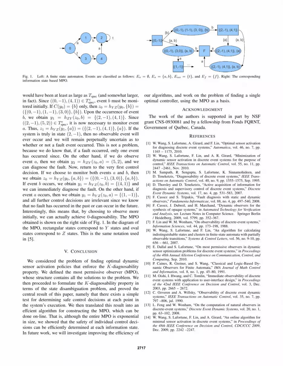
Fig. 1. Left: A finite state automaton. Events are classified as follows: Eo = ∅, Es = {a, b}, Euo = {t}, and Ef = {f}. Right: The correspondinginformation state based MPO.

would have been at least as large as Tspec (and somewhat larger,in fact). Since ((0,−1), (4, 1)) ∈ T e

spec, event b must be moni-tored initially. If C(y0) = {b} only, then z0 = hY Z(y0, {b}) =({(0,−1), (1,−1), (3, 0)}, {b}). Upon the occurrence of eventb, we obtain y1 = hZY (z0, b) = {(2,−1), (4, 1)}. Since((2,−1), (5, 2)) ∈ T e

spec, it is now necessary to monitor eventa. Thus, z1 = hY Z(y1, {a}) = ({(2,−1), (4, 1)}, {a}). If thesystem is truly in state (2,−1), then no observable event willever occur and we will remain perpetually uncertain as towhether or not a fault event occurred. This is not a problem,because we do know that, if a fault occurred, only one eventhas occurred since. On the other hand, if we do observeevent a, then we obtain y2 = hZY (z0, a) = (5, 2), and wecan diagnose the fault. Now, return to the very first controldecision. If we choose to monitor both events a and b, thenwe obtain z0 = hY Z(y0, {a, b}) = ({(0,−1), (3, 0)}, {a, b}).If event b occurs, we obtain y1 = hY Z(z0, b) = {(4, 1)} andwe can immediately diagnose the fault. On the other hand, ifevent a occurs, then we obtain y1 = hY Z(z0, a) = {(1,−1)},and all further control decisions are irrelevant since we knowthat no fault has occurred in the past or can occur in the future.Interestingly, this means that, by choosing to observe moreinitially, we can actually achieve 0-diagnosability. The MPOobtained is shown on the right side of Fig. 1. In the diagram ofthe MPO, rectangular states correspond to Y states and ovalstates correspond to Z states. This is the same notation usedin [5].

V. CONCLUSION

We considered the problem of finding optimal dynamicsensor activation policies that enforce the K-diagnosabilityproperty. We defined the most permissive observer (MPO),whose structure contains all the solutions to the problem. Wethen proceeded to formulate the K-diagnosability property interms of the state disambiguation problem, and proved thecentral result of this paper, namely that there exists a simpletest for determining safe control decisions at each point inthe system’s execution. We then translated this result into aneffcient algorithm for constructing the MPO, which can bedone on-line. That is, although the entire MPO is exponentialin size, we showed that the safety of individual control deci-sions can be efficiently determined at each information state.In future work, we will investigate improving the efficiency of

our algorithms, and work on the problem of finding a singleoptimal controller, using the MPO as a basis.

ACKNOWLEDGMENT

The work of the authors is supported in part by NSFgrant CNS-0930081 and by a fellowship from Fonds FQRNT,Government of Quebec, Canada.

REFERENCES

[1] W. Wang, S. Lafortune, A. Girard, and F. Lin, “Optimal sensor activationfor diagnosing discrete event systems,” Automatica, vol. 46, no. 7, pp.1165 – 1175, 2010.

[2] W. Wang, S. Lafortune, F. Lin, and A. R. Girard, “Minimization ofdynamic sensor activation in discrete event systems for the purpose ofcontrol,” IEEE Transactions on Automatic Control, vol. 55, no. 11, pp.2447 –2461, Nov. 2010.

[3] M. Sampath, R. Sengupta, S. Lafortune, K. Sinnamohideen, andD. Teneketzis, “Diagnosability of discrete event systems,” IEEE Trans-actions on Automatic Control, vol. 40, no. 9, pp. 1555–1575, Sep. 1995.

[4] D. Thorsley and D. Teneketzis, “Active acquisition of information fordiagnosis and supervisory control of discrete event systems,” DiscreteEvent Dynamic Systems, vol. 17, no. 4, pp. 531–583, 2007.

[5] F. Cassez and S. Tripakis, “Fault diagnosis with static and dynamicobservers,” Fundamenta Informaticae, vol. 88, no. 4, pp. 497–540, 2008.

[6] F. Cassez, J. Dubreil, and H. Marchand, “Dynamic observers for thesynthesis of opaque systems,” in Automated Technology for Verificationand Analysis, ser. Lecture Notes in Computer Science. Springer Berlin/ Heidelberg, 2009, vol. 5799, pp. 352–367.

[7] F. Lin and W. M. Wonham, “On observability of discrete-event systems,”Information Sciences, vol. 44, pp. 173–198, 1988.

[8] W. Wang, S. Lafortune, and F. Lin, “An algorithm for calculatingindistinguishable states and clusters in finite-state automata with partiallyobservable transitions,” Systems & Control Letters, vol. 56, no. 9-10, pp.656 – 661, 2007.

[9] E. Dallal and S. Lafortune, “On most permissive observers in dynamicsensor optimization problems for discrete event systems,” in Proceedingsof the 48th Annual Allerton Conference on Communication, Control, andComputing, Sep. 2010.

[10] P. Caines, R. Greiner, and S. Wang, “Classical and Logic-Based Dy-namic Observers for Finite Automata,” IMA Journal of Math Controland Information, vol. 8, no. 1, pp. 45–80, 1991.

[11] M. Oishi, I. Hwang, and C. Tomlin, “Immediate observability of discreteevent systems with application to user-interface design,” in Proceedingsof the 42nd IEEE Conference on Decision and Control, vol. 3, Dec.2003, pp. 2665 – 2672.

[12] C. Ozveren and A. Willsky, “Observability of discrete event dynamicsystems,” IEEE Transactions on Automatic Control, vol. 35, no. 7, pp.797 –806, jul. 1990.

[13] L. Feng and W. Wonham, “On the computation of natural observers indiscrete-event systems,” Discrete Event Dynamic Systems, vol. 20, no. 1,pp. 63–102, 2008.

[14] W. Wang, S. Lafortune, F. Lin, and A. Girard, “An online algorithm forminimal sensor activation in discrete event systems,” in Proceedings ofthe 48th IEEE Conference on Decision and Control, CDC/CCC 2009,Dec. 2009, pp. 2242 –2247.

2717