a dynamic model for rule induction tasks
TRANSCRIPT
455
⁄0022-2496/02 $35.00
© 2002 Elsevier Science (USA)All rights reserved.
Journal of Mathematical Psychology 46, 455–485 (2002)doi:10.1006/jmps.2001.1400
A Dynamic Model for Rule Induction Tasks
Tom Verguts
We thank William Batchelder, Siegfried Dewitte, Martin Schrepp, and Francis Tuerlinckx for theiruseful comments on the topic or on previous versions of this paper.Address correspondence and reprint requests to Tom Verguts, Department of Psychology,Tiensestraat 102, 3000 Leuven, Belgium. E-mail: [email protected].
University of Leuven
Eric Maris
University of Nijmegen
and
Paul De Boeck
University of Leuven
In this paper, a model for performance on rule induction tasks (e.g., itemson intelligence tests) is developed. The model simultaneously specifies distri-butions for response times and response accuracies on an item-by-item basis.It is dynamic in the sense that it can be used to specify and test different waysof learning throughout a test. Three versions of the general model (i.e., withthree different learning rules) are described and the fit of these versions isinvestigated in two datasets on solving number series. The results indicatethat one of these versions (one of the learning rules) is better at accountingfor the data. © 2002 Elsevier Science (USA)
INTRODUCTION
This paper develops a model to account for human problem solving in ruleinduction tasks. The core assumption in this model is that solving items of this typeconsists of sampling a sequence of possible solution rules (or solution principles).For example, possible rules for solving integrals are ‘‘substitute’’ and ‘‘decomposeinto fraction.’’ Such rules are sampled until a useful one is found.Each rule is assumed to have a certain level of activation. The probability ofsampling a rule as well as the time needed to perform this sampling depend on theactivation of that particular rule. Activations of individual rules can change duringproblem solving and this is the way that learning is incorporated in the model.

Probability distributions for accuracy and response time are derived from theseassumptions.It has been amply demonstrated that the process of finding solutions in complexcognitive tasks (such as rule induction tasks) is affected by one’s history of successesand failures (i.e., learning). For example, this has been demonstrated for anagramproblems (Kaplan & Schoenfeld, 1966; Lemay, 1972; White, 1988), the water jarstask (Shore, Koller, & Dover, 1994), the stick building task (Lovett & Anderson,1996; Lovett & Schunn, 1999), insight problems (Duncker, 1945; Maier & Burke,1966), and baseball knowledge (Wiley, 1998). This paper presents a model forstudying this phenomenon in more detail than is possible with traditional models.The model is applied to number series performance. One detailed model for(letter) series performance was proposed by Simon and Kotovsky (1963). Thismodel consists of an algorithm describing the various steps people are presumed tofollow in solving such problems. Most research on this task builds on that paper(Kotovsky & Simon, 1973; Holzmann, Pellegrino, & Glaser, 1982, 1983; Schrepp,1995). The model is a static model, in the sense that the probability of solving aparticular item remains unchanged throughout the test.An influential series of models that can capture learning throughout a test is theseries of ACT models by Anderson and colleagues (e.g., Anderson, 1983, 1993;Anderson & Lebiere, 1998). One important difference between their models and theone we present is that ours is simpler, which makes it to easier to (a) estimateparameters, (b) investigate goodness-of-fit of the model, and (c) empirically distin-guish different versions of the model with different substantive psychological inter-pretations.The remainder of the paper consists of five parts. In the first section (NumberSeries Task) we briefly discuss the rule induction task that is used in our two exper-imental studies described later. This task is introduced in an early phase because theexplanation of the model itself builds on this task. In the second section (Model),we derive the relevant equations. In the third section (Study 1) the model is appliedto number series data without a time limit. In the fourth section (Study 2) the modelis applied to number series data with a time limit. Finally, we close the paper with ageneral discussion.
NUMBER SERIES TASK
Each item of our task is a number series1 such as ‘‘3, 5, 7, 9, 11, 13.’’
1Mathematically, the term ‘‘number series’’ is not completely appropriate since the task involvedconcerns number sequences, not series. However, we follow the tradition in this literature and refer tothis task as a number series.
The number series always consists of six numbers. Each such item can be describedaccording to a certain logical rule. Four rule types are used: addition, Fibonacci,interpolation, and multiplication. An example of the addition type is ‘‘3, 4, 6, 9,13, 18.’’ In an item of this type, the increment between two consecutive numbers isitself incremented by one (so the sequence of increments is +1, +2, +3, +4, +5).The increment between two successive increments is always equal to one, but items
456 VERGUTS, MARIS, AND DE BOECK
can differ in starting number and initial increment. In items of the Fibonacci type,each number is the sum of the previous two. The first two numbers are chosenarbitrarily, with the second number larger than the first. An example is ‘‘2, 4, 6, 10,16, 26.’’ In items of the interpolation type, two series are interpolated, each one witha constant increment rule: An example is ‘‘2, 5, 6, 8, 10, 11,’’ which is a mix of thesequences ‘‘2, 6, 10, ...’’ and ‘‘5, 8, 11, ... .’’ In items of the multiplication type, theincrement is always multiplied by a constant value. An example is ‘‘1, 3, 7, 15,31, 63.’’ The multiplier is always equal to 2. Our rule induction task is constructedby creating a test of 50 such items, with items of the four types intermixed. Thecomplete set of items is presented twice so in fact 100 items are presented to theparticipants. More details on test administration are presented later on.
MODEL
In the first subsection (Response Process) the general model is presented. Thesecond subsection (Activation Dynamics) describes the three versions of the model,each corresponding to a different learning rule. In the third subsection (TimeLimits), we discuss the changes to the model that are required when a time limit peritem is imposed. In the fourth subsection (Estimating and Testing the Model), wediscuss how to estimate the parameters of the model and how to investigate itsgoodness-of-fit.
Response Process
Suppose K possible rules can be used to solve all items of a certain test. In thenumber series example of the previous subsection, K=4; this number is imposed bythe experimenter. When shown an item, one of these rules is sampled. Sampling aparticular rule is conceptualized as a race between the different rules (e.g., Marley,1989). Specifically, each rule k is supposed to have a finishing time that is exponen-tially distributed with hazard rate parameter wk. That is, if Vk denotes the finishingtime for rule k, its probability density function (PDF) is given by p(Vk)=wk exp(−wkVk). The first rule to finish the race is sampled and tried out by the par-ticipant. For example, if the addition rule described in the previous section wins therace, the participant tries to apply this rule to the item at hand. It is easily demon-strated (e.g., Ross, 2000, p. 295, Exercise 7) that if the race times Vk are statisticallyindependent, then the probability that rule k is tried out is given by
Pr(rule k chosen)=wk
;m wm,
where the summation is taken over all rules.If the rule that is sampled turns out to be inapplicable to the item, the process isstarted anew. That is, a new race is set up between all possible rules and the fastestrule is again tried out. Note that the sampling is with replacement. If the correct rulewins the race, it is applied and the solution process is terminated. However, somerules may be incorrect but still lead to a termination of the iterated samplingprocess. For example, suppose a participant incorrectly concludes that the series
DYNAMIC MODEL FOR RULE INDUCTION 457
‘‘1, 3, 5, 7, 9’’ is governed by the rule ‘‘each number is the previous one multipliedby three.’’ In this case, the sampling process will stop, although the correct rule isnot found. Another possible ‘‘rule’’ which may stop the solution process is theanswer ‘‘I don’t know.’’ In this case, the participant decides she cannot solve theitem and goes on to the next one. We aggregate all such misleading rules (mislead-ing in the sense that they incorrectly lead to a termination of the solution process)into an additional response category (K+1), with corresponding activation wK+1.Hence, the race between rules is iterated until either the correct rule is found or oneof the misleading ones wins the race.Let us denote the activation of the correct rule by wC (so C ¥ {1, ..., K}). Then,this iterated sampling process can be conceptualized as a three-state Markov chain,with the three states corresponding to (a) having sampled the correct rule (denotedstate C), (b) having sampled the misleading rule (denoted state M), and (c) havingsampled one of the remaining rules (a rule with an index k ¥ {1, ..., C−1,C+1, ..., K}), denoted state R. The transition probability matrix is given by
: C M R
C 1 0 0
M 0 1 0
R pC pM 1−pC−pM
(1)
where pC=wC/;K+1k=1 wk and pM=wK+1/;K+1
k=1 wk. The process starts in state R.It is now possible to derive the probability of success and the response-time dis-tribution on an item-by-item basis. Let us introduce the item index i (=1, ..., I).This index is attached to the variables introduced earlier. For example, wki nowdenotes the activation of rule k at the presentation of item i. Further, let C(i)denote the correct rule number for item i. For example, if rule 2 is the correct onefor item i=1, then C(1)=2. Then, the probability of sampling the correct rule atitem i is equal to pC(i) i.An item is solved correctly if the chain eventually ends up in state C (rather thanstate M). Let Xi (with realizations xi) denote the accuracy variable. That is, Xi=1if item i is solved correctly and Xi=0 otherwise. It then follows from elementarystochastic process theory (e.g., Ross, 1996, Proposition 4.4.2) that
Pr(Xi=1)=pC(i) i
pC(i) i+p(K+1) i=
wC(i) iwC(i) i+w(K+1) i
. (2)
Let Ti (with realizations ti) be the variable denoting the decision time. This is thetime needed to reach either one of the two states C orM. It is now possible to showthat
p(Ti=ti | Xi=xi)=p(Ti=ti)=(wC(i) i+w(K+1) i) exp(−(wC(i) i+w(K+1) i) ti), (3)
so Ti follows an exponential distribution. This is shown in Appendix A (Result 3).
458 VERGUTS, MARIS, AND DE BOECK
Combining Eqs. (2) and (3), we get the following PDF for the responses (accuraciesand decision times) to all I items jointly:
p(data)=DI
i=1Pr(Xi=xi) p(Ti=ti | Xi=xi)
=DI
i=1(wC(i) i)xi (w(K+1) i)1−xi exp[−(wC(i) i+w(K+1) i) ti]. (4)
The probabilities in these equations are conditional on the parameters wki. Thus,given these parameters, the different Xi and Ti are all statistically independent.The observed response time is assumed to be composed of two parts, a decisiontime and a motor response time. Until now, we have only focused on the decisiontime. The motor response time is the time needed to transform a decision into amotor response (pressing a button, for instance). For simplicity, the motor responsetime is assumed to be a person-specific constant tre. The observed response time canhence be denoted Ti, re=Ti+tre. In our analysis, we first estimate the person-specificconstants tre and then calculate Ti=Ti, re−tre. These Ti are then treated as observeddecision times that are assumed to be governed by Eq. (4).Although the assumption of a constant motor-response time is an oversimplifi-cation, it should be noted that for the tasks modeled the motor response time isrelatively small as compared to the decision time. Also, it is not our intention todescribe the response time distribution in great detail. Rather, we will try to modelthe change in mean response time (the mean taken over blocks of items) to find outwhat this change tells us about the process of solving number series.
Activation Dynamics
Activations wki may change over items as a function of experience and feedback.In general, activations change according to the formula
wki=f(wk(i−1)). (5)
That is, the current activation is a function of the activation on the previous item. Itmay be that wki also depends on a few parameters, but this is implicit in Eq. (5). Wewill consider three special cases of f.
1. The activations are constant throughout; that is, wki=wk(i−1). Theresulting model will be called the constant model in the remainder.
2. The activations of the responses wki change according to the formula
wki=˛awk(i−1)+(1−a) h if item i−1 is of type k and Xi−1=1,awk(i−1) otherwise.
(6)
This model will be called the incremental model, which is shorthand for ‘‘incremen-tal learning model.’’ In Eq. (6), 0 [ a [ 1 and h \ 0. This equation states that if the
DYNAMIC MODEL FOR RULE INDUCTION 459
previous item (i−1) is of type k and that item is solved correctly, the activation ofrule k increases. Otherwise, the activation decreases. For example, if an item is notsolved correctly, then all activation values will decrease. Equation (6) is similar toformulas that were used in earlier mathematical models of learning (e.g., Bush &Mosteller, 1955; Luce, 1959).If a rule is not useful or cannot be found for some time, its activation willdecrease at an exponential rate. In particular, the activation of the (K+1)thresponse, which is sometimes used but is never useful, can be written as w(K+i) i=a i−1w(K+1) 1. This assumption may be unrealistic because the tendency to give up(which is one of the responses in the (K+1)th category) may increase rather thandecrease over time. However, if the giving-up option is not often chosen, the modelmay very well be appropriate (see the Results and Discussion sections of Studies 1and 2).The parameters wk1 refer to the initial biases of a participant. If wk1 is high, theparticipant is likely to sample rule k right from the start when responding to thefirst item. The parameter h partly determines how strongly rules are activated by aprevious successful application. Indeed, if h is high, the activation wki will increasestrongly after successfully solving an item (cf. Eq. (6)). As for the parameter a, thehigher it is (the closer to 1), the slower the activations change, as can be seen fromEq. (6), and hence the slower the response distributions change. The parameter amay therefore be called a stability parameter.
3. The third model is the all-or-none model, in which the activations wki canbe in only two possible states. We formalize this learning rule as follows:
wki=˛h if rule k is used successfully earlier,wk1 otherwise.
(7)
When a rule is activated, it jumps to the point h and never leaves that position. Thisexplains the name ‘‘all-or-none model.’’ Note that, in this model, the activation ofthe (K+1)th response is constant throughout the test (w(K+1) i=w(K+1) 1 for allitems i).The model in Eq. (7) does not correspond in detail to the all-or-none modelspresented earlier in the literature (e.g., Restle, 1962, 1965). However, the old all-or-none models and the present one share the philosophy that a learner can be in oneof only two states, corresponding to unlearned (or weakly active) and learned (orstrongly active), respectively. A more detailed comparison between the current andthe older all-or-none models is provided in the General Discussion. Figure 1 pre-sents examples of how activities develop in all three models (constant, incremental,and all-or-none).
Time Limits
Suppose only a limited time, say 15 seconds, is allowed per item. Then, everyparticipant has only 15−tre s (15 minus the motor response time) to think. Thisthreshold (15−tre) will be denoted by y.
460 VERGUTS, MARIS, AND DE BOECK
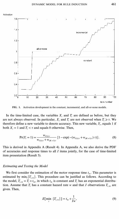
FIG. 1. Activation development in the constant, incremental, and all-or-none models.
In the time-limited case, the variables Xi and Ti are defined as before, but theyare not always observed. In particular, Xi and Ti are not observed when Ti \ y. Wetherefore define a new variable to denote accuracy. This new variable, Yi, equals 1 ifboth Xi=1 and Ti < y and equals 0 otherwise. Then,
Pr(Yi=1)=wC(i) i
wC(i) i+w(K+1) i{1− exp(−(wC(i) i+w(K+1) i) y)}. (8)
This is derived in Appendix A (Result 4). In Appendix A, we also derive the PDFof accuracies and response times to all I items jointly, for the case of time-limiteditem presentation (Result 5).
Estimating and Testing the Model
We first consider the estimation of the motor response time tre. This parameter isestimated by mini{Ti, re}. This procedure can be justified as follows. According tothe model, Ti, re=Ti+tre, in which tre is constant and Ti has an exponential distribu-tion. Assume that Ti has a constant hazard rate w and that I observations Ti, re aregiven. Then,
E[mini{Ti, re}]=tre+
1Iw, (9)
DYNAMIC MODEL FOR RULE INDUCTION 461
since the minimum has itself an exponential distribution with parameter Iw. Thisresult shows that the estimator mini{Ti, re} is biased, but also that the bias is small ifthe sample size (I) is sufficiently large. It might be suspected that this procedure issusceptible to outliers at the left-hand side of the response-time distribution, but wewill show that there are no such outliers in our data.After subtracting the estimated motor response times from the observed responsetimes, these adjusted response times are entered in the likelihood function, which isthen maximized. Thus, maximum likelihood estimates are computed on accuraciesand adjusted response times. The maximization is performed by a protected steepestascent algorithm which is described in Appendix B. The estimation can be per-formed for every participant separately or for all participants together. The secondprocedure will be used when parameters are restricted to be equal acrossparticipants to increase parsimony of the model.For the constant and the all-or-none models, parameters will be estimated foreach participant separately. For the incremental model, parameters are estimatedfor all participants together. This is because the parameter a is restricted to be equalacross participants. Restricting a to be equal across participants is motivated by thefact that we found this parameter to vary little over participants. Different wk1(initial activation) and h parameters are assumed for every participant. The hparameter is assumed to be constant across rules. Hence, the resulting number ofparameters of the incremental model is (K+2) P+1, where P denotes the numberof participants. After this restriction, the incremental model has only one parametermore than the all-or-none model. Specifically, the incremental and all-or-nonemodels now have (K+2) P+1 and (K+2) P parameters, respectively.The model will be tested using the parametric bootstrap procedure (Davison &Hinkley, 1997). This procedure is as follows:
1. Using the estimated parameter vector t=(h, a, ..., w(K+1) 1) for a givenperson, a new data matrix D rep, n is generated N times (n=1, ..., N).
2. Consider a statistic S (different possibilities for S will be discussed later).Let Sobs denote the statistic S as evaluated in the observed data. For each data set n,we check whether S rep, n \ Sobs, where S rep, n denotes the statistic evaluated at the nthreplicated data set D rep, n.
3. The proportion of times that S rep, n \ Sobs is our bootstrapped p-value.Small values (e.g., below .05) indicate that the model is inadequate.
The idea of this procedure is to approximate the true sampling distribution of thestatistic S by replacing the true parameter vector (t) with its estimate (t) and to usethe resulting distribution as the reference distribution for the observed value of S.Thus, the bootstrapped p-value is an approximation of the actual p-value.Recording the number of times that S rep, n \ Sobs (see Step 2) is useful for good-ness-of-fit statistics in which a large Sobs indicates a bad fit and a small Sobs indi-cates a good fit (e.g., a Pearson chi-square statistic). This will be called a one-sidedbootstrap test in the following. However, it is not appropriate for statistics in whichboth very small and very large values of Sobs indicate a bad fit. In these cases, the
462 VERGUTS, MARIS, AND DE BOECK
p-value will be calculated two-sided instead of one-sided. Specifically, in thetwo-sided case we will check whether
|S rep, n−S rep| \ |Sobs−S rep|,
for all n=1, ..., N. In this case, if the p-value is low, this indicates that Sobs is farfrom the mean of S rep (which is denoted by S rep). In the following, when a teststatistic is presented, it will also be indicated whether a one- or two-sided test isperformed. The value of N, the number of bootstrap samples, is set to 100 (perperson and per statistic).
STUDY 1
In this section, we apply the model to a data set on number series performancewithout a time limit. At this point, a note concerning the uniqueness of the rules isin order. Korossy (1998) discusses the fact that even in a very restricted class ofitems there are often many rules that are possible for a single item. He advisesresearchers to tell participants the class of rules under study, so participants canpick one of the intended rules. However, this is neither necessary nor advisable inthe present study, for the following reasons. First, it is not advisable since theecological validity of the task would suffer: Telling the intended rules would makethe test much easier and the test could hardly be called a rule discovery test in thiscase. Second, it is not necessary because we ask participants to state the rule theyare using, rather than to complete the item series. Hence, if people indeed usealternative rules, we would notice this. However, this did not happen in the studieswe report on here. People either use the rules we used to construct the item series orrules that are incorrect or inaccurate.
Method
Material. The number series task was described earlier. There are four ruletypes: addition, Fibonacci, interpolation, and multiplication. In items of the inter-polation type, the series can in principle be nonincreasing, but we constructed theitems so that this did not occur (i.e., the series is always increasing). For the mul-tiplication type, the multiplier used is always equal to 2. The reason for these twoconventions will be explained, later.A test of 50 items is constructed and presented twice in identical order. Hence,I=100 items are presented. The different rule types are introduced gradually. Initems 1 to 10, the addition and Fibonacci types are used, each rule being used 5times out of 10. ln items 11 to 20, the interpolation type is added to these two:Addition, Fibonacci, and interpolation rules are used 2, 4, and 4 times, respectively,in this set of 10 items. In items 21 to 30, the addition and interpolation types areused, each rule used 5 times out of 10. In items 31 to 40, the multiplication type isadded to these two, with addition, interpolation, and multiplication being used 3, 3,and 4 times, respectively. Finally, in items 41 to 50 all 4 types are used, and addi-tion, Fibonacci, interpolation, and multiplication are used 2, 3, 2, and 3 timesrespectively. The exact same sequence is repeated for items 51–100. The samesequence of items is presented to each participant.
DYNAMIC MODEL FOR RULE INDUCTION 463
Procedure. Items are presented on a computer screen. The participant is askedto find the rule involved in the item. If the rule is found, the participant has to pressthe spacebar, which causes a box to cover the item. In this way, we try to enforcethat the participant can no longer think about the rule after pressing the space bar.She should type the rule in the box that appears after pressing the space bar. Itshould be stressed that the participant does not have to complete the number series,but simply has to describe the rule she thinks is the correct one. Hence, the processof finding the rule is separated from the process of applying it. The participant hasunlimited time to type in the rule.In the instructions, the procedure that is required of the participant (typing arule) is illustrated with two examples of number series involving a constant incre-ment (e.g., 2, 5, 8, 11, 14, 17), a rule that is not used in the actual test. Also, it ismentioned that two series may be intermixed: In this way, a hint is given about theinterpolation series. This hint is given because in a pilot experiment it had turnedout that the interpolation rule is very difficult to discover without a hint.After the participant has typed his/her rule, the same series appears again withtwo extra numbers added. For example, if the series is ‘‘1, 3, 5, 7, 9, 11,’’ theextended series would be ‘‘1, 3, 5, 7, 9, 11, 13, 15.’’ This way, the participantreceives feedback about the rule he/she typed because he/she can check whetherthe rule he/she used is in accord with the extended series. The time available tolook at the extended series is unlimited.Each participant is tested separately. Instructions are presented on the computerscreen, and if everything is clear the participant starts solving the items. Theexperimenter does not intervene but always stays in the room. Participants are toldthat they are performing in a response time experiment and that they should workas fast as possible without compromising accuracy.
Data coding. After data collection, two types of data are registered per item,response time and accuracy, the latter indicating whether or not the rule describedis the correct one. The coding is such that the participant is credited with a 1 if thecorrect principle is described even if some details in the description are incorrect. Tomake this more concrete, we now give some details on the scoring of the responsesto the different rule types. For the addition type, a rule description is consideredcorrect if it refers to increasing increments. For example, if the participant describesas a rule ‘‘+1, +2, +3, +4, ...,’’ this is considered correct, but also if the partici-pant writes ‘‘+2,+3,+4,+5, ...’’ for that item. For a Fibonacci item, a response isconsidered correct if there is some reference to the two previous numbers. Forexample, correct descriptions would be ‘‘add two numbers to obtain the next one,’’‘‘the previous number and the last one give the following one,’’ and so on. In thelast description, adding is considered to be the default operation, and this is whythis description is considered correct too, even though there is no explicit referenceto the operation that should be performed. If a participant explicitly mentions anincorrect operation performed on the last two numbers, this would be consideredan incorrect response. For an interpolation item, a response is considered correct ifthere is some reference to the mixing of two series. For example, in the series ‘‘1, 4,5, 7, 9, 10, 13,’’ if a participant’s rule description is ‘‘for the odd numbers, +4, and
464 VERGUTS, MARIS, AND DE BOECK
for the even numbers, also +4,’’ this is considered correct because there is a clearreference to the mixing of series, even though the exact rule is not correct (for theeven numbers, the relevant rule is +3 rather than+4). For a multiplication item, aresponse is considered correct if there is some reference to the multiplication ofincrements. In the item ‘‘3, 4, 6, 10, 18, 34,’’ correct rule descriptions would be‘‘+1, +2, +4, +8, ...,’’ ‘‘multiply the differences by two,’’ ‘‘differences are increas-ing powers of two,’’ and so on. Some people also used the mathematically equiva-lent rule, ‘‘Each number is the previous one times two plus a constant.’’ This wasalso considered correct. Finally, the additional response category (K+1) wasscored if the participant gave an incorrect rule or typed a give-up response such as‘‘I don’t know.’’
Participants. Eight persons participated for a small monetary reward. Theywere students of the University of Leuven who had responded to an advertisement.
Trends. Trends in the data will be examined. The two learning models (incre-mental and all-or-none) predict that accuracy (probability of success) will increaseand response time will decrease over time. This is not predicted by the constantmodel. To investigate this, all instances of each item type are divided into twoblocks as follows: The addition items that were presented in the first half of the testare assigned to Block 1, and the addition items that were presented in the secondhalf are assigned to Block 2. The same procedure is followed for the Fibonacci,interpolation, and multiplication items.We look at the mean accuracy and mean response times over these two blocks,for every (person, item type) pair separately, and report the number of times thatthe difference is in the direction expected by the two learning models. That is,according to the two learning models, accuracy should be higher in the secondblock than in the first and response time should be shorter in the second block thanin the first.Note that investigating the trend in the accuracies is exactly analogous to inves-tigating the frequency of occurrence of the (K+1)th category, since, in this study,choosing the (K+1)th category implies Xi=0, and vice versa. The same will nolonger be true in the next study, where a time limit is imposed.
Goodness-of-fit-statistics. Here, we describe the goodness-of-fit statistics thatwill be used in the parametric bootstrap procedure to test the model. For the firststatistic to be developed, smaller blocks are constructed than those described in theprevious subsection in order to perform more fine-grained analyses. For item-typeaddition, blocks are constructed as follows: Addition items in the first quarter ofthe test are assigned to Block 1, those in the second quarter to Block 2, those in thethird quarter to Block 3, and those in the fourth quarter to Block 4. A similar pro-cedure is followed for Fibonacci and interpolation items. For type multiplication,the two-block structure of the previous paragraph is maintained since there are nomultiplication items in the first quarter of the test. Hence, for addition, Fibonacci,and interpolation, four blocks are constructed, and for multiplication items onlytwo.
DYNAMIC MODEL FOR RULE INDUCTION 465
Let the item type (addition, Fibonacci, interpolation, or multiplication, in thatorder) be indexed by k=1, ..., 4. The first statistic to be used is defined as
Qacc(k)=CB
b=1
[Xbk−E(Xbk)]2
E(Xbk). (10)
Here, Xbk denotes the mean accuracy of all items of type k within block b. Thevariable E(Xbk) is its expectation, which is calculated as
E(Xbk)=1nbk
Ci in block band of type k
E(Xi), (11)
where nbk denotes the number of items of type k in block b and E(Xi) is used as ashorthand notation for E(Xi | X1, ..., Xi−1). The dependence is needed because suc-cesses on previous items influence current success through the activation values wki(see Eqs. (6) and (7)). The summation in Eq. (11) is taken over all items belongingto block b and of type k (e.g., items 1, ..., 25 for b=1 and item type addition). Thisstatistic will be called the Pearson accuracy statistic because it is modeled after thefamiliar Pearson chi-square statistic. We will perform a one-sided bootstrap test forthis statistic.A similar discrepancy measure is calculated for response times,
Qtime(k)=CB
b=1
[Tbk−E(Tbk)]2
E(Tbk). (12)
In Eq. (12),
E(Tbk)=1nbk
Ci in block band of type k
E(Ti),
where E(Ti) is used as a shorthand notation for E(Ti | X1, ..., Xi−1). Again, thedependence on X1, ..., Xi−1 is needed because successes on previous items partiallydetermine the wki values which are needed to calculate E(Ti). The statistic Qtime willbe called the Pearson response time statistic.The third and fourth types of statistic are inspired by a statistical test proposedby Suppes and Ginsberg (1963), which was intended to check a critical aspect of anall-or-none learning model (see our General Discussion for a more elaboratedescription of that model). Their work was concerned with the paired-associatelearning paradigm, and they noted that, prior to learning the (all-or-none) connec-tion between a word and its associated word, successes on the stimulus word shouldbe binomially distributed. This implies that the correct response probabilities arestationary: Prior to learning the association between words, the probability of suc-cessfully answering an item remains constant. Suppes and Ginsberg developed a testfor this aspect of the data. Similar statistics can be constructed in our case, with thedifference that we will check participants’ behavior after a rule has been learned,rather than before. These statistics will be called stationary statistics. One will beconstructed for the accuracy data and one for the response time data.
466 VERGUTS, MARIS, AND DE BOECK
To construct the stationarity statistic for item type k, define item ik to be the firstitem of type k on which a participant gives a correct answer (i.e., xik=1 and xi=0for all items i < ik of type k). Divide all items i > ik of type k into blocks of five:The first five items i of type k for which it holds that i > ik constitute Block 1, thenext five items constitute Block 2, and so on. Suppose there are B such blocks, andlet Xbk be the mean accuracy of type-k items in a block b. (Note that this definitionof Xbk is different from that used in Eqs. (10)–(12).) Finally, let Xk be the meanaccuracy of all items i > ik of type k. Then, the stationarity accuracy statistic isdefined as
Gacc(k)=1B
CB
b=1(Xbk−Xk)2. (13)
The motivation for this statistic is as follows. Under the constant model, allaccuracies Xi involved in this statistic are obtained from the same distribution,namely, a Bernoulli distribution with probability wC(i) 1/(wC(i) 1+w(K+1) 1). Note thatthe item index i=1 can be chosen in this case since the activation values are thesame for all items of the same type under the constant model. Under the all-or-nonemodel, all accuracies are from a Bernoulli distribution with probabilityh/(h+w(K+1) 1). The important thing to note is that in both cases (constant and all-or-none models), these probabilities are the same for all items of rule type k. Hence,under the constant and all-or-none model, the probability of success does notchange for items i > ik of type k.On the other hand, for the incremental model, let the correct rule for item i berule k (so C(i)=k). Then, item accuracies arise from Bernoulli distributions withthe probability of a correct response being
wkiwki+w(K+1) i
=a i−1wk1+h(1−a); i−2
j=0 ajI{k}(i−1−j) Xi−1−j
(a i−1wk1+h(1−a); i−2j=0 a
jI{k}(i−1−j) Xi−1−j)+a i−1w(K+1) 1, (14)
where I{k}(i) is an indicator function which is equal to 1 if item i is of type k and iszero otherwise. The equality in Eq. (14) can be derived by applying mathematicalinduction on Eq. (6). Contrary to the probabilities for the constant and the all-or-none models, the probabilities for the incremental model change after every newitem.The motivation for the statistic in Eq. (13) is now that there will be less varia-bility among the Xi if they all arise from the same distribution (as for the constantand all-or-none models) than if they all arise from different distributions (as for theincremental model). The statistic in Eq. (13) is intended as a measure of the varia-bility of the Xi’s. Under the constant and the all-or-none models, this statistic willbe smaller than under the incremental model. Although this is difficult to deriveanalytically, it is easily demonstrated by simulations. Hence, this statistic can beexpected to be diagnostic in distinguishing between the constant and all-or-nonemodels, on the one hand, and, on the other hand, the incremental model.Strictly speaking, we could also use the data before the first success to distinguishbetween the incremental and the all-or-none models. This is not done here for tworeasons. First, the activations wki of the incremental model change only very weakly
DYNAMIC MODEL FOR RULE INDUCTION 467
during this period, so there is not a big difference with the all-or-none model in thisphase. Second, we are especially interested in the type of learning after a rule is usedcorrectly for the first time; namely, are activations fixed as in the all-or-none modelor variable as in the incremental model? Therefore, the data before the first successdo not bear much on our main point of interest.In a similar manner, we introduce the stationarity response-time statistic,
Gtime(k)=1B
CB
b=1(Tbk−Tk)2, (15)
in which Tbk and Tk are defined in an analogous way as Xbk and Xk are in Eq. (13).Again, this statistic is expected to be smaller under the constant and the all-or-nonemodels than under the incremental model for a similar reason to that outlined inthe previous paragraphs.
Results and Discussion
Two participants are excluded from the analysis because they gave up more andmore often and faster and faster in the course of test taking. This pattern of datacannot be captured by any of the models, so we decided not to analyze these data.Hence, only the 6 participants who did not give up (or not often) were considered inthe following analyses.
Descriptive statistics. Mean accuracies (over items) range (over persons) from.620 to .950. The overall mean accuracy is .887; its standard deviation (SD) overpersons equals 0.136. Mean response times (over items) range (over persons) from4.259 to 25.437 s. The overall mean response time is 15.163 s, and its SD overpersons equals 7.138. Mean accuracies per item type are 1, .924, .779, and .821 foraddition, Fibonacci, interpolation, and multiplication, respectively. Addition andFibonacci items seem to be quite easy. In the following analyses, we will focus oninterpolation and multiplication items because they allow for learning to show up inboth accuracy and response time data.All minimum response times are within one standard deviation of the meanresponse time, calculated for every person separately. This illustrates our statementin the context of Eq. (9) that there are no outliers at the low end of the responsetime scale that can harm the estimation of tre.
Trends. For the accuracy data, we performed 6×4=24 (number of persons ×number of item types) comparisons between performances in the first and in thesecond block of items. Of these 24 comparisons, seven are in the direction predictedby the learning models (accuracy higher in the second block). Three out of theseseven comparisons are statistically significant at the level .05. In 16 comparisons,the accuracies in Blocks 1 and 2 are equal. This is mainly due to people who havenull or perfect scores throughout the test for a certain item type (which occurred 13times out of 16). For one person–item type combination, there was higher accuracyin the first block than in the second.
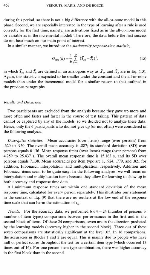
468 VERGUTS, MARIS, AND DE BOECK
For the response time data, all 24 comparisons are in the direction predicted bythe two learning models (response time is lower in Block 2). Of these, 11 are signi-ficant at the .05 level. Hence, these trends in the data, especially in the responsetime data, seem to speak in favor of the two learning models. The accuracy datamay not be appropriate for distinguishing between the two learning models and theconstant model because of a very high overall accuracy.
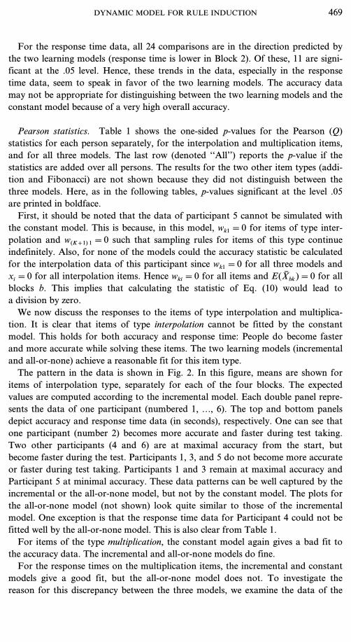
Pearson statistics. Table 1 shows the one-sided p-values for the Pearson (Q)statistics for each person separately, for the interpolation and multiplication items,and for all three models. The last row (denoted ‘‘All’’) reports the p-value if thestatistics are added over all persons. The results for the two other item types (addi-tion and Fibonacci) are not shown because they did not distinguish between thethree models. Here, as in the following tables, p-values significant at the level .05are printed in boldface.First, it should be noted that the data of participant 5 cannot be simulated withthe constant model. This is because, in this model, wk1=0 for items of type inter-polation and w(K+1) 1=0 such that sampling rules for items of this type continueindefinitely. Also, for none of the models could the accuracy statistic be calculatedfor the interpolation data of this participant since wk1=0 for all three models andxi=0 for all interpolation items. Hence wki=0 for all items and E(Xbk)=0 for allblocks b. This implies that calculating the statistic of Eq. (10) would lead toa division by zero.We now discuss the responses to the items of type interpolation and multiplica-tion. It is clear that items of type interpolation cannot be fitted by the constantmodel. This holds for both accuracy and response time: People do become fasterand more accurate while solving these items. The two learning models (incrementaland all-or-none) achieve a reasonable fit for this item type.The pattern in the data is shown in Fig. 2. In this figure, means are shown foritems of interpolation type, separately for each of the four blocks. The expectedvalues are computed according to the incremental model. Each double panel repre-sents the data of one participant (numbered 1, ..., 6). The top and bottom panelsdepict accuracy and response time data (in seconds), respectively. One can see thatone participant (number 2) becomes more accurate and faster during test taking.Two other participants (4 and 6) are at maximal accuracy from the start, butbecome faster during the test. Participants 1, 3, and 5 do not become more accurateor faster during test taking. Participants 1 and 3 remain at maximal accuracy andParticipant 5 at minimal accuracy. These data patterns can be well captured by theincremental or the all-or-none model, but not by the constant model. The plots forthe all-or-none model (not shown) look quite similar to those of the incrementalmodel. One exception is that the response time data for Participant 4 could not befitted well by the all-or-none model. This is also clear from Table 1.For items of the type multiplication, the constant model again gives a bad fit tothe accuracy data. The incremental and all-or-none models do fine.For the response times on the multiplication items, the incremental and constantmodels give a good fit, but the all-or-none model does not. To investigate thereason for this discrepancy between the three models, we examine the data of the
DYNAMIC MODEL FOR RULE INDUCTION 469
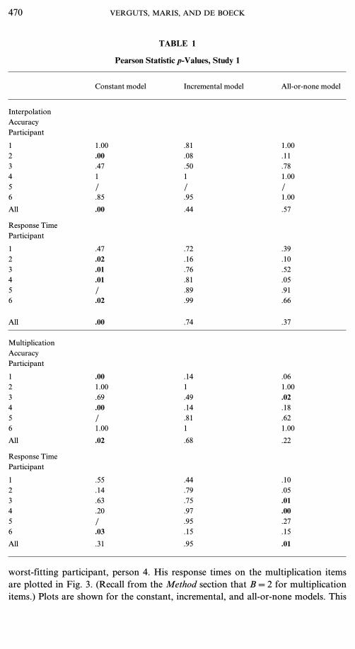
TABLE 1
Pearson Statistic p-Values, Study 1
Constant model Incremental model All-or-none model
InterpolationAccuracyParticipant
1 1.00 .81 1.002 .00 .08 .113 .47 .50 .784 1 1 1.005 / / /6 .85 .95 1.00
All .00 .44 .57
Response TimeParticipant
1 .47 .72 .392 .02 .16 .103 .01 .76 .524 .01 .81 .055 / .89 .916 .02 .99 .66
All .00 .74 .37
MultiplicationAccuracyParticipant
1 .00 .14 .062 1.00 1 1.003 .69 .49 .024 .00 .14 .185 / .81 .626 1.00 1 1.00
All .02 .68 .22
Response TimeParticipant
1 .55 .44 .102 .14 .79 .053 .63 .75 .014 .20 .97 .005 / .95 .276 .03 .15 .15
All .31 .95 .01
worst-fitting participant, person 4. His response times on the multiplication itemsare plotted in Fig. 3. (Recall from the Method section that B=2 for multiplicationitems.) Plots are shown for the constant, incremental, and all-or-none models. This
470 VERGUTS, MARIS, AND DE BOECK
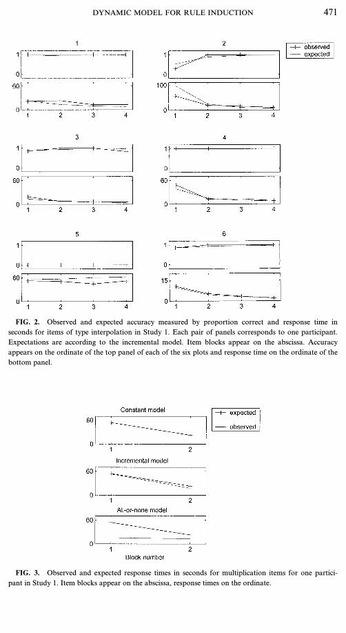
FIG. 2. Observed and expected accuracy measured by proportion correct and response time inseconds for items of type interpolation in Study 1. Each pair of panels corresponds to one participant.Expectations are according to the incremental model. Item blocks appear on the abscissa. Accuracyappears on the ordinate of the top panel of each of the six plots and response time on the ordinate of thebottom panel.
FIG. 3. Observed and expected response times in seconds for multiplication items for one partici-pant in Study 1. Item blocks appear on the abscissa, response times on the ordinate.
DYNAMIC MODEL FOR RULE INDUCTION 471

participant finds the correct rule very quickly in Block 1, so the all-or-none modelpredicts that there is no speedup from Block 1 to Block 2. Of course, the constant
TABLE 2
Stationarity Statistic p-values, Study 1
Constant model Incremental model All-or-none model
InterpolationAccuracyParticipant
1 1.00 .43 .382 .13 .23 .483 .74 .72 .754 1.00 1.00 .985 / / /6 .34 .22 .34
All .06 .11 .10
Response TimeParticipant
1 .83 .71 .362 .15 .17 .073 .18 .15 .174 .01 .75 .005 / / /6 .60 .42 .05
All .07 .21 .00
MultiplicationAccuracyParticipant
1 .00 .10 .022 .58 .88 .903 .57 .58 .834 .00 .29 .115 / .23 .466 .59 .59 .55
All .03 .55 .34
Response TimeParticipant
1 .90 .78 .012 .93 .53 .493 .46 .31 .114 .46 .24 .145 / .56 .566 .07 .09 .10
All .41 .16 .02
472 VERGUTS, MARIS, AND DE BOECK
model also predicts no speedup. Only the incremental model can capture the factthat this participant becomes faster after the first correct application of a rule.Another question is why the all-or-none model puts its expected response time solow (see the third plot in Fig. 3), rather than placing it in between the observedresponse times, just like in the constant model. The reason is that type-multiplica-tion items have to share the same value h with other item types. Therefore, thevalue h, which determines the expected response time, is a compromise between‘‘fast’’ (addition, Fibonacci) and ‘‘slow’’ (interpolation, multiplication) item types.Until now, we have found clear evidence against the constant model but the evi-dence favoring either the incremental or the all-or-none model was less clear. Ingeneral, the incremental model was supported better (see Table 1), but not always.
Stationarity statistics. We now consider the stationarity statistics, which wereconstructed with the aim of distinguishing between the incremental and the all-or-none models. Again, we restrict our discussion to the interpolation and multiplica-tion items. Table 2 reports the p-values for the three models. Participant 5 solvedno items of interpolation type, so calculating this statistic is not meaningful here.For the interpolation items, the accuracy data do not distinguish between thethree models. However, from the response time data, it is clear that the incrementalmodel does a better job than either the constant or the all-or-none model. Thissuggests that people still learn after the first use of a solution principle.
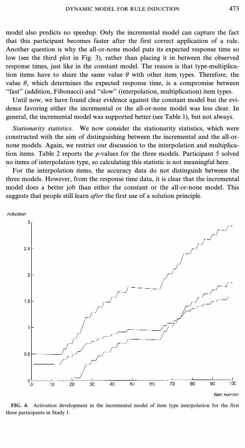
FIG. 4. Activation development in the incremental model of item type interpolation for the firstthree participants in Study 1.
DYNAMIC MODEL FOR RULE INDUCTION 473
For the accuracy data of the multiplication items, the constant model again turnsout to fit worse than the other two. For the response time data, the all-or-nonemodel fits worst (see the row ‘‘All’’ for multiplication items in Table 2).Our tentative conclusion from these data is that the incremental model performsbetter than either of the other two. However, this could be ascribed to two sourcesof differences between this model and the other two. It may be the case that theincremental model fits better because rule activation develops gradually over time(as we suggest). An alternative explanation, however, is that it is better because it isthe only model that allows for forgetting or gradually diminishing activation.However, in the present data, this second explanation is implausible because theestimated parameter a is quite high (a=.998). Hence, if a certain rule is not usedfor a while, its activation will diminish very slowly. Figure 4 shows the estimatedactivation profiles for the first three participants for the rule type interpolation (theprofiles for the other three participants are very similar). One can see that indeed ifrule activation diminishes, it does so very slowly. It should be noted that Eq. (6)seems to imply that, with a high a value, rule activation also increases very slowlyafter successfully using a rule. However, this is not the case (as is clear from Fig. 4),because the parameter h can compensate for a high a value. For the incrementalmodel, the mean estimated h parameter is 61.844, with a minimum value of 31.684.Hence, our incremental activation account of the data seems warranted.
STUDY 2
Method
The material and data coding are the same as in Study 1. The only difference inthe procedure is that only 15 s are allowed to solve an item. If that limit is reachedthe extended number series is shown as in Study 1, and the participant can proceedto the next item by pressing the space bar.
Participants. Eight persons participated for a small monetary reward. All personswere different from those in Study 1. They were students that had responded to anadvertisement.
Trends. Trends in the data are investigated as in the previous study.
Goodness-of-fit statistics. The Pearson Q statistic for the new accuracy variableYi is defined in the same way as the statistic for Xi was defined earlier. Analogousstatistics for response times are not used in this study. This is because preliminaryanalyses indicated that the time limit of 15 s is quite severe, and the response-time differences are not diagnostic for distinguishing between the three models.A stationarity statistic is also not used here because it turned out not to bediagnostic in preliminary analyses of these data.
Results and Discussion
Descriptive statistics. Mean accuracies (over items) range (over persons) from.500 to .670. The overall mean accuracy is .568, its standard deviation (SD) overpersons equals 0.055. As expected, the mean accuracy is much lower than inStudy 1, due to the time limit.
474 VERGUTS, MARIS, AND DE BOECK
The mean response time is calculated over all response times smaller than 15 s.Response-time means (over items) range (over persons) from 5.240 to 9.240 s. Theoverall mean response time is equal to 7.246 s; its SD equals 1.286. As expected,both the mean and the standard deviation are lower than in Study 1. The propor-tions of success are .831, .672, .259, and .473 for, respectively, addition-, Fibonacci-,interpolation-, and multiplication-type items.All minimum response times are within two standard deviations of the meanresponse time, calculated for every person separately. Again, this illustrates ourstatement in the context of Eq. (9), that there are no outliers to disturb theestimation of tre.
Trends. For the accuracy data, 8×4=32 comparisons can be performed. Ofthese, 21 are in the direction predicted by the learning models (higher accuracy inthe second block than in the first). Eight of these 21 comparisons are significant atthe level .05. In six of the comparisons, the mean accuracy is equal across blocks,and in five the mean accuracy is higher in the first block than in the second. Noneof these differences is statistically significant.For the response time data, the truncated data are included to perform thefollowing calculations. Twenty-seven comparisons out of 32 result in faster responsetimes in the second block than in the first. Of these 27, 12 are statistically signifi-cant. Four comparisons are in the inverse direction, and for one comparison theresponse times are equal in both blocks (equality of mean response time is possiblebecause of the truncation).We now look at the trend in the proportion of incorrect responses given beforethe deadline (i.e., the (K+1)th response category). In three out of eight compari-sons this proportion decreases over blocks. In three comparisons the number isequal, and in two the number increases from the first to the second block. None ofthese differences is statistically significant. Hence, the proportion of incorrectresponses does not decrease strongly.
Pearson statistics. Table 3 shows p-values for the Pearson statistic applied toaccuracy data for the three models and for the interpolation and multiplicationitems. If one looks at the last row (denoted ‘‘All’’) of Table 3 for the accuracy andresponse-time data, it can be seen that the incremental model has a better fit thanthe all-or-none model has. This test of the all-or-none model has lower power thanthe test of the incremental model has (due to two fewer participants (5 and 7) beingused in the computation of this statistic for the all-or-none model, for a similarreason as that excluding participant 5 in Study 1). Despite this, Table 3 shows thatthe incremental model does better than the all-or-none model does. Also, theincremental model is better than the constant model.As in the previous study, one might wonder whether the better fit of the incre-mental model is due to its ability to explain forgetting rather than to graduallyincreasing activation. Again, it turns out that the latter explanation is probablycorrect, since the estimated a is again quite high (a=0.9995). In case the first partof the learning rule in Eq. (6) applies (for increasing activation), this is com-pensated by relatively high h-values (mean estimated h=188.016, with a minimum
DYNAMIC MODEL FOR RULE INDUCTION 475

TABLE 3
Pearson Statistic p-values, Study 2
Constant model Incremental model All-or-none model
AccuracyInterpolationParticipant
1 .00 .06 .112 .01 .06 .263 .98 .54 .024 .11 .33 .345 .00 .06 /6 .01 .00 .007 1.00 1.00 /8 .01 .27 .33
All .00 .02 .00
MultiplicationParticipant
1 .94 .40 .002 .92 .69 .033 .71 .78 .054 .18 .27 .275 1.00 .80 /6 .70 .34 .647 .92 .86 /8 .83 .84 .02
All .95 .90 .00
of 112.073). The activation profile for the different participants is similar to thatshown in Fig. 4. There is incremental learning but little if any forgetting. So why dowe include the a parameter at all, rather than use a model where there is onlyincremental learning and no forgetting? The main reason is the interpretability ofthe h parameter in the present formulation of the incremental model. Specifically,suppose that beyond a certain item i, all items are solved correctly. In that case, itholds that limiQ. ; k wki=h. Hence, h can then be interpreted as the maximumactivation that is possible. No such interpretation is possible for the h parameter ifthe a parameter is taken out of the model.
To summarize our findings from both studies, we note that a constant model isinadequate for these data: People do learn while solving this test. Also, the all-or-none learning rule does not seem to account for the data as well as the incrementalmodel does.
GENERAL DISCUSSION
We have developed a general model to account for speed and accuracy data inrule-induction tasks and have shown that this model gives an adequate fit to several
476 VERGUTS, MARIS, AND DE BOECK
aspects of our data. We have formulated, fitted, and tested three specific models intwo contexts (with and without a time limit). The constant model was clearly ina-dequate, and of the two other models, the incremental model fitted better than theall-or-none model. To end this paper, we discuss two limitations of our model andrelate our work to some other research traditions.
Stimulus Information
We have assumed that only the activations of rules that have been built up in thepast determine which response is chosen: There is no direct information from thestimulus itself. A more general model might be one in which certain stimulusaspects cooperate in determining a response. Although this is certainly a relevantdirection to extend the model, we did not incorporate it here because the stimulithemselves usually lend few hints about the correct rule involved. For example,consider the two series
4 7 11 16 22 29
and
5 6 9 11 13 16.
The first is an example of the addition rule and the second an example of theinterpolation rule. The most obvious way to solve these items is to simply try outthe different possible rules rather than to look for specific cues that may differen-tiate between different item types. A point relevant to this argument is that we tookcare to avoid any cues that might distinguish between different item types. Forexample, only items of the interpolation type can in principle show a nonincreasingitem series (e.g., 4, 7, 5, 10, 6, 13). However, as mentioned earlier, the item series weconstructed for these studies were all increasing. Hence, this could not help partici-pants in making a choice between rules. A second example is that the numbers usedin multiplication-type items can increase very quickly if large multipliers are used,but we used only the multiplier 2, the smallest one possible.
Other Learning Mechanisms
A second limitation concerns our localization of learning in the activation ofsolution rules. Other ways to become more proficient in number series performancewould be faster encoding of the number series or faster and more accurate rulechecking (a process that is ignored in the present model). Our model cannot dealwith these kinds of learning. However, in our opinion, in the number series taskthese processes can probably be performed relatively quickly and accurately incomparison with the problem of finding the correct rule.
Dynamics of Test Behavior
Earlier, we noted the fact that many cognitive task analyses assume that nochange takes place during test performance. The untenability of this assumption incognitive testing is most dramatically shown in participants’ behavior on the waterjars task (e.g., Dover & Shore, 1991; Luchins, 1942; Shore et al., 1994). The samepoint was also clearly demonstrated in the present paper by the bad fit of the con-stant model. The misfit was more subtle with number series than with the water jars
DYNAMIC MODEL FOR RULE INDUCTION 477
task, so that we had to resort to statistical methods to show this. On the otherhand, our test represents a more realistic situation in the sense that it more closelyresembles a typical intelligence test.
Existing Learning Models
Some learning models have been proposed in the experimental literature, and wenow make a comparison between our work and a few of these.
The incremental vs all-or-none learning controversy. In the fifties and sixties,there was a debate on whether learning is incremental or all-or-none. We have alsochosen to call two of our models incremental and all-or-none. However, thesemodels, especially the all-or-none model, differ from the ones presented earlier (e.g.,Restle, 1962, 1965). We will discuss the similarities and differences between ourmodels and two well-known earlier learning models, the linear operator model andthe one-element stimulus sampling model.
Consider a paired-associate learning experiment. A set of pairs of words is to belearned, and the first words of the set are presented repeatedly. At each presenta-tion of a word, the participant is required to recall the other word of the pair. Aftera response, the correct answer is provided by the experimenter. The linear operatormodel assumes that at each presentation the probability Pn of providing the correctmissing word, at the nth presentation of that word, is equal to
Pn=(1−h) Pn−1+h.
This model is similar to our incremental model in that the probability of successincreases gradually. However, there are also important differences. First, there is nodependence on previous performance in the linear operator model (i.e., Xi−1).Second, the linear operator model operates directly on probabilities, whereas weassume that the probability of success depends on underlying activations thatchange over time. And third, no response time predictions are derived from thelinear operator model, in contrast to ours. Despite the differences, we think it isnevertheless useful to place our incremental model in this tradition, since it sharesthe basic idea of gradually increasing probabilities of success.On the other hand, the one-element model (or the all-or-none model) is amodel allowing only two states; the ‘‘unlearned’’ and the ‘‘learned’’ states. In theunlearned state, people guess the correct word and have a probability g of guessingthe correct one, where g is usually the reciprocal of the number of response options.After every item processed in the unlearned state, there is a fixed probability ofjumping to the learned state. Once in the learned state, the participant never leavesthat state and solves the item correctly with probability 1. This model differs fromour all-or-none model in important ways. First, in our model, the initial state (i.e.,if the activation of the rule is wk1) is not a completely unlearned state because thereis still some probability wk1/(w(K+1) 1+wk1) of finding the correct rule (for rule typek). On the other hand, in the one-element model, nothing at all is known in theunlearned state, and successful item performance can occur solely through correctguessing. Second, in our model, in the learned state (i.e., if the activation of a rule isequal to h) the probability of success is h/(w(K+1) 1+h), rather than 1. And third, in
478 VERGUTS, MARIS, AND DE BOECK
the one-element model, the event of jumping to the learned state is independent ofthe performance on the previous item. Despite these differences, we have chosen tocall our model an all-or-none model as well, because the two models (ourall-or-none model and the one-element model) share the same basic idea that learn-ing is a ‘‘discontinuous’’ phenomenon; that is, a chunk of knowledge is eitherknown or unknown.
Modern learning models. Recently, interest in learning has revived, and manynew learning models have been proposed. Many of these new models are of a con-nectionist type (e.g., Dragoi & Staddon, 1999; Gluck & Bower, 1988; Kruschke,1992). A related but nonconnectionist model is the dynamic version of the fuzzylogic model (Friedman, Massaro, Kitzis, & Cohen, 1995). Friedman et al. (1995)and Kitzis, Kelley, Berg, Massaro, and Friedman (1998) present theoretical andempirical comparisons between several of these models. None of these recentmodels adhere to all-or-none learning rules. Instead, they all use some type ofincremental learning rule. For example, one often-used rule is the backpropagationlearning rule in neural networks (e.g., Ballard, 1995). In backpropagation learning,the learner is given the correct answer, and weights in the network are optimallyadapted such as to minimize the difference between the correct and the statedanswer. However, the empirical validity of these learning rules is seldom testedexplicitly. Methods proposed in this paper may prove to be useful for makingdetailed comparisons between different learning rules.
APPENDIX A
Derivations
In this appendix, we derive some observations stated in the main text. The chro-nology of the text is followed. The item index i will be dropped whenever this doesnot lead to confusion.Suppose K+1 responses perform a race, in which each response races with a timethat is independent and exponentially distributed with parameter (hazard rate) wk.Then, it is an elementary exercise in probability theory to show that the race timeand the choice are statistically independent in this case (see Ross, 2000, p. 295,Exercise 7). Further, it also follows from that exercise that the probability of thekth rule winning the race equals wk/[;K+1
k=1 wk].Using the definition wtot=;K+1
k=1 wk, we recall that pC=wC/wtot, as in the maintext, and we introduce the notation pK+1=wK+1/wtot and pstop=pC+pK+1=(wC+wK+1)/wtot. The variable wtot denotes the total activation, pC is the probabilityof sampling the correct rule, pK+1 is the probability of sampling the misleading rule,and pstop is the probability that the sampling process stops (i.e., the probability ofsampling the correct or the misleading rule).We first discuss the time-unlimited case. In the main text, it is already noted thatthe probability of success equals
Pr(X=1)=wC
wC+wK+1, (A1)
DYNAMIC MODEL FOR RULE INDUCTION 479
where C denotes the number of the correct rule. Our first result concerns thedistribution of the number of sampled rules in a given item, denoted J (withrealizations j). It turns out that J has a geometric distribution with parameter pstop.
Result 1. Pr(J=j |W=x)=Pr(J=j)=pstop(1−pstop) j−1.
Proof.
Pr(J=j | X=x)=Pr(J=j, X=x)Pr(X=x)
=(1−pstop) j−1 p
xCp1−xK+1
wxCw1−xK+1
wC+wK+1
=(1−pstop) j−1 pstop. L
The second equality of the proof follows from applying Eq. (A1) to Pr(X=x).The next result states that the total decision time t for a given item, conditionalon the number of rules that are sampled (j), is Gamma distributed with parametersj and wtot.
Result 2. p(T=t | J=j, X=x)=p(T=t | J=j)=Gamma(j, wtot).
Proof. The variable T is the sum of j component times. Every component timeis the winning time of a race between K+1 independent exponential randomvariables. From Ross (2000, p. 295, Exercise 7), it follows that the distribution ofeach component time is independent of x. Therefore, T (the sum of the componenttimes) is also independent of x. This proves the first equality. Now, since everycomponent time is distributed as an exponential with parameter wtot, it follows thatT is distributed as a Gamma with parameters j and wtot. This proves the secondequality. L
The next result shows that the decision time follows an exponential distributionwith hazard rate (wC+wK+1). We introduce the moment-generating function of T,denoted byMT(s). The idea of the proof is due to McGill (1963).
Result 3. p(T=t | X=x)=p(T=t)=(wC+wK+1) exp[−(wC+wK−1) t].
Proof.
MT | X=x(s)=C.
j=1Pr(J=j) MT | X=x, J=j(s)
=C.
j=1(1−pstop) j−1 pstop 1
wtotwtot−s2 j
=wC+wK+1wC+wK+1−s
.
The second equality of the proof follows from Result 2. Hence, p(T | X=x) is anexponential distribution with parameter (wC+wK+1). L
480 VERGUTS, MARIS, AND DE BOECK
The following two results are referred to in the subsection ‘‘Time Limits’’ of themain text.
Result 4. Pr(Y=1)=(wC/(wC+wK+1)) {1− exp(−(wC+wK+1) y)}.
Proof.
Pr(Y=1)=Pr(X=1 & T < y)=Pr(X=1 | T < y) Pr(T < y)
=wC
wC+wK+1{1− exp(−((wC+wK+1) y)}. L
We now derive the PDF of accuracies and response times to all I items jointly forthe case of time-limited item presentation. We first define, for item i,
ui=˛ti if ti < yy otherwise.
Then, we can state and prove the following result.
Result 5. p(data)=<i [wxiC(i) iw
1−xi(K+1) i]
I(0, y)(ui) exp[−(wC(i) i+w(K+1) i) ui].
The symbol I denotes an indicator function, where I(0, y)(u)=1 if 0 < u < y andI(0, y)(u)=0 otherwise.
Proof. With time-limited presentation, the variables Ti and Xi are sometimesnot observed, namely, when Ti \ y. The variables Ti with Ti \ y are said to be trun-cated. We define the variable Oi which indicates whether Ti and Xi are observed(Oi=1 if Ti < y) or not (Oi=0 if Ti \ y). We denote the set of items with ti < y asD1 and the items with ti \ y as D0. The probability density of allobservations, including the observations where Ti \ y, can be written as
p(data)=5DI
i=1Pr(Oi=oi)6×5 D
i ¥ D1
p(Xi=xi, Ti=ti | Oi=1)6
=5 Di ¥ D0
[1−Fi(y)]6×5 Di ¥ D1
Fi(y)6×5 Di ¥ D1
p(Xi=xi, Ti=ti, Oi=1)Pr(Oi=1)
6 ,(A2)
where the symbol Fi( ) denotes the cumulative distribution of the response time foritem i. We can rewrite (A2) as
p(data)=Di ¥ D0
[1−Fi(y)] Di ¥ D1
p(Xi=xi, Ti=ti)
=Di ¥ D0
exp[−(wC(i) i+w(K+1) i) y]
× Di ¥ D1
(wC(i) i)xi (w(K+1) i)1−xi exp[−(wC(i) i+w(K+1) i) ti]
=Di[(wC(i) i)xi (w(K+1) i)1−xi]I(0, y)(ui) exp[−(wC(i) i+w(K+1) i) ui]. L
Note that xi is not observed for items with ti \ y. However, in this case xi doesnot appear in the PDF because I(0, y)(ui)=0 for these items.
DYNAMIC MODEL FOR RULE INDUCTION 481
APPENDIX B
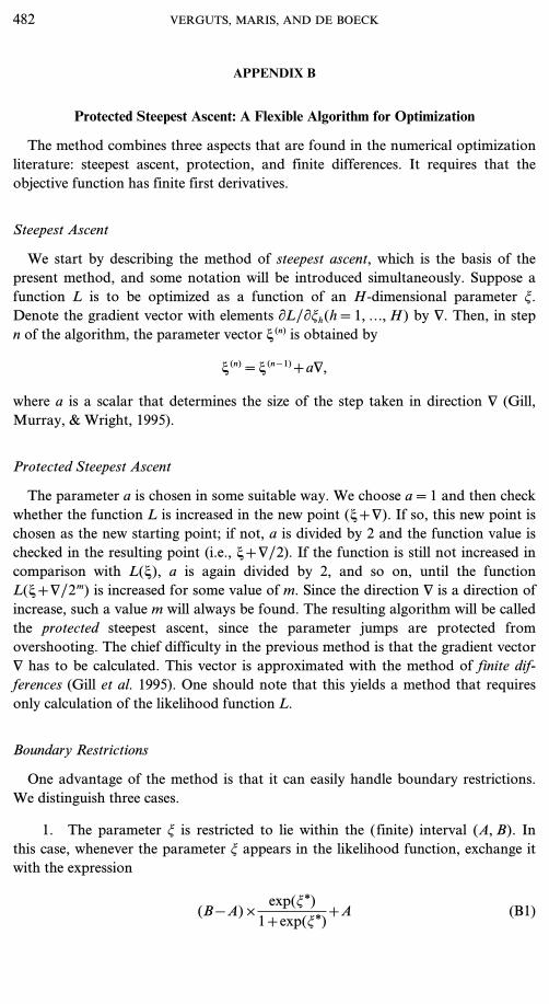
Protected Steepest Ascent: A Flexible Algorithm for Optimization
The method combines three aspects that are found in the numerical optimizationliterature: steepest ascent, protection, and finite differences. It requires that theobjective function has finite first derivatives.
Steepest Ascent
We start by describing the method of steepest ascent, which is the basis of thepresent method, and some notation will be introduced simultaneously. Suppose afunction L is to be optimized as a function of an H-dimensional parameter t.Denote the gradient vector with elements “L/“th(h=1, ..., H) by N. Then, in stepn of the algorithm, the parameter vector t (n) is obtained by
t (n)=t (n−1)+aN,
where a is a scalar that determines the size of the step taken in direction N (Gill,Murray, & Wright, 1995).
Protected Steepest Ascent
The parameter a is chosen in some suitable way. We choose a=1 and then checkwhether the function L is increased in the new point (t+N). If so, this new point ischosen as the new starting point; if not, a is divided by 2 and the function value ischecked in the resulting point (i.e., t+N/2). If the function is still not increased incomparison with L(t), a is again divided by 2, and so on, until the functionL(t+N/2m) is increased for some value of m. Since the direction N is a direction ofincrease, such a value m will always be found. The resulting algorithm will be calledthe protected steepest ascent, since the parameter jumps are protected fromovershooting. The chief difficulty in the previous method is that the gradient vectorN has to be calculated. This vector is approximated with the method of finite dif-ferences (Gill et al. 1995). One should note that this yields a method that requiresonly calculation of the likelihood function L.
Boundary Restrictions
One advantage of the method is that it can easily handle boundary restrictions.We distinguish three cases.
1. The parameter t is restricted to lie within the (finite) interval (A, B). Inthis case, whenever the parameter t appears in the likelihood function, exchange itwith the expression
(B−A)×exp(tg)1+exp(tg)
+A (B1)
482 VERGUTS, MARIS, AND DE BOECK
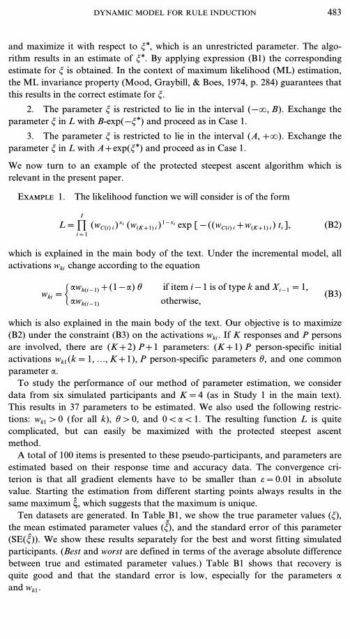
and maximize it with respect to tg, which is an unrestricted parameter. The algo-rithm results in an estimate of tg. By applying expression (B1) the correspondingestimate for t is obtained. In the context of maximum likelihood (ML) estimation,the ML invariance property (Mood, Graybill, & Boes, 1974, p. 284) guarantees thatthis results in the correct estimate for t.
2. The parameter t is restricted to lie in the interval (−., B). Exchange theparameter t in L with B-exp(−tg) and proceed as in Case 1.
3. The parameter t is restricted to lie in the interval (A,+.). Exchange theparameter t in L with A+exp(tg) and proceed as in Case 1.
We now turn to an example of the protected steepest ascent algorithm which isrelevant in the present paper.
Example 1. The likelihood function we will consider is of the form
L=DI
i=1(wC(i) i)xi (w(K+1) i)1−xi exp [−((wC(i) i+w(K+1) i) ti], (B2)
which is explained in the main body of the text. Under the incremental model, allactivations wki change according to the equation
wki=˛awk(i−1)+(1−a) h if item i−1 is of type k and Xi−1=1,awk(i−1) otherwise,
(B3)
which is also explained in the main body of the text. Our objective is to maximize(B2) under the constraint (B3) on the activations wki. If K responses and P personsare involved, there are (K+2) P+1 parameters: (K+1) P person-specific initialactivations wk1(k=1, ..., K+1), P person-specific parameters h, and one commonparameter a.To study the performance of our method of parameter estimation, we considerdata from six simulated participants and K=4 (as in Study 1 in the main text).This results in 37 parameters to be estimated. We also used the following restric-tions: wk1 > 0 (for all k), h > 0, and 0 < a < 1. The resulting function L is quitecomplicated, but can easily be maximized with the protected steepest ascentmethod.A total of 100 items is presented to these pseudo-participants, and parameters areestimated based on their response time and accuracy data. The convergence cri-terion is that all gradient elements have to be smaller than e=0.01 in absolutevalue. Starting the estimation from different starting points always results in thesame maximum t, which suggests that the maximum is unique.Ten datasets are generated. In Table B1, we show the true parameter values (t),the mean estimated parameter values (t), and the standard error of this parameter(SE(t)). We show these results separately for the best and worst fitting simulatedparticipants. (Best and worst are defined in terms of the average absolute differencebetween true and estimated parameter values.) Table B1 shows that recovery isquite good and that the standard error is low, especially for the parameters aand wk1.
DYNAMIC MODEL FOR RULE INDUCTION 483

TABLE B1
Parameter Estimates for I=100
Best-fitting participant Worst-fitting participant
Parameter t t SE(t) t t SE(t)
a 0.990 0.991 0.002 0.990 0.991 0.002h 1.000 0.908 0.379 5.000 5.513 0.968w1, 1 0.100 0.124 0.056 0.100 0.130 0.078w2, 1 0.050 0.063 0.025 0.050 0.060 0.046w3, 1 0.060 0.080 0.045 0.060 0.094 0.059w4, 1 0.020 0.019 0.016 0.020 0.059 0.073wK+1 0.100 0.089 0.021 0.100 0.102 0.030
REFERENCES
Anderson, J. R. (1983). The architecture of cognition. Hillsdale, NJ: Erlbaum.
Anderson, J. R. (1993). Rules of the mind. Hillsdale, NJ: Erlbaum.
Anderson, J. R. (1996). ACT: A simple theory of complex cognition. American Psychologist, 51,355–365.
Anderson, J. R., & Lebiere, C. (Eds.) (1998). The atomic components of thought.Mahwah, NJ: LawrenceErlbaum.
Ballard, D. H. (1997). An introduction to natural computation. Cambridge, MA: MIT Press.
Bush, R. R., & Mosteller, F. (1955). Stochastic models for learning. New York: Wiley.
Davison, A. C., & Hinkley, D. V. (1997). Bootstrap methods and their applications. Cambridge, MA:Cambridge University Press.
Dover, A., & Shore, B. M. (1991). Giftedness and flexibility on a mathematical set-breaking task. GiftedChild Quarterly, 35, 99–124.
Dragoi, V., & Staddon, J. E. R. (1999). The dynamics of operant conditioning. Psychological Review,106, 20–61.
Duncker, K. (1945). On problem solving. Psychological Monographs, 58, No. 5.
Friedman, D., Massaro, D. W., Kitzis, S. N., & Cohen, M. M. (1995). A comparison of learning models.Journal of Mathematical Psychology, 39, 164–178.
Gill, P. E., Murray, W., & Wright, M. H. (1995). Practical optimization. London: Academic Press.
Gluck, M. A., & Bower, G. H. (1988). From conditioning to category learning: An adaptive networkmodel. Journal of Experimental Psychology: General, 117, 227–247.
Holzman, T. G., Pellegrino, J. W., & Glaser, R. (1982). Cognitive dimensions of numerical ruleinduction. Journal of Educational Psychology, 74, 360–373.
Holzman, T. G., Pellegrino, J. W., & Glaser, R. (1983). Cognitive variables in series completion. Journalof Educational Psychology, 75, 603–618.
Kaplan, I. T., & Schoenfeld, W. N. (1966). Oculomotor patterns during the solution of visuallydisplayed anagrams. Journal of Experimental Psychology, 72, 447–451.
Kitzis, S. N., Kelley, H., Berg, E., Massaro, D. W., & Friedman, D. (1998). Broadening the tests oflearning models. Journal of Mathematical Psychology, 42, 327–355.
Korossy, K. (1998). Solvability and uniqueness of linear-recursive number sequence tasks. Methods ofPsychological Research, 3 [www.mpr-online.de].
484 VERGUTS, MARIS, AND DE BOECK

Kotovsky, K., & Simon, H. A. (1973). Empirical tests of a theory of human acquisition of concepts forsequential patterns. Cognitive Psychology, 4, 399–424.
Kruschke, J. K. (1992). ALCOVE: An exemplar-based connectionist model of category learning.Psychological Review, 99, 22–44.
Lemay, E. H. (1972). Anagram solutions as a function of task variables and solution word models.Journal of Experimental Psychology, 92, 65–68.
Lovett, M. C., & Anderson, J. R. (1996). History of success and current context in problem solving.Cognitive Psychology, 31, 168–217.
Lovett, M. C., & Shunn, C. D. (1999). Journal of Experimental Psychology: General, 128, 107–130.
Luce, R. D. (1959). Individual choice behavior. New York: Wiley.
Luchins, A. S. (1942). Mechanization in problem solving—The effect of Einstellung. PsychologicalMonographs, 54.
Maier, N. R., & Burke, R. J. (1966). Test of the concept of ‘‘availability of functions’’ in problemsolving. Psychological Reports, 19, 119–125.
Marley, A. A. J. (1989). A random utility family that includes many of the classical models and hasclosed form choice probabilities and choice reaction times. British Journal of Mathematical andStatistical Psychology, 42, 13–36.
McGill, W. J. (1963). Stochastic latency mechanisms. In R. D. Luce, R. R. Bush, and E. Galanter (Eds.),Handbook of mathematical psychology (Vol. 1, pp. 309–360). New York: Wiley.
Mood, A. M., Graybill, F. A., and Boes, D. C. (1974). Introduction to the theory of statistics. Singapore:McGraw–Hill.
Restle, F. (1962). The selection of strategies in cue learning. Psychological Review, 69, 329–343.
Restle, F. (1965). Significance of all-or-none learning. Psychological Bulletin, 64, 313–325.
Ross, S. M. (1996). Stochastic processes. New York: Wiley.
Ross, S. M. (2000). Introduction to probability models. San Diego: Academic Press.
Schrepp, M. (1995). Modeling interindividual differences in solving letter series completion problems.Zeitschrift für Psychologie, 203, 173–188.
Shore, B. M., Koller, M., and Dover, A. (1994). More from the water jars: A reanalysis of problem-solving performance among gifted and nongifted children. Gifted Child Quarterly, 38, 179–183.
Simon, H. A., and Kotovsky, K. (1963). Human acquisition of concepts for sequential patterns.Psychological Review, 70, 534–546.
Suppes, P., and Ginsberg, R. (1963). A fundamental property of all-or-none models, binomialdistribution of responses prior to conditioning, with application to concept formation in children.Psychological Review, 70, 139–161.
White, H. (1988). Semantic priming of anagram solutions. American Journal of Psychology, 101,383–399.
Wiley, J. (1998). Expertise as mental set: The effects of domain knowledge in creative problem solving.Memory and Cognition, 26, 716–730.
Received: May 23, 2000; published online: January 10, 2002
DYNAMIC MODEL FOR RULE INDUCTION 485