rule formats for distributivity
TRANSCRIPT
Rule Formats for Distributivity?
Luca Aceto1, Matteo Cimini1, Anna Ingolfsdottir1,MohammadReza Mousavi2, and Michel A. Reniers3
1 ICE-TCS, School of Computer Science, Reykjavik University,Menntavegur 1, IS 101 Reykjavik, Iceland
2 Department of Computer Science, Eindhoven University of Technology,P.O. Box 513, NL-5600 MB Eindhoven, The Netherlands
3 Department of Mechanical Engineering, Eindhoven University of Technology,P.O. Box 513, NL-5600 MB Eindhoven, The Netherlands
Abstract. This paper proposes rule formats for Structural OperationalSemantics guaranteeing that certain binary operators are left distributivewith respect to a set of binary operators. Examples of left-distributivitylaws from the literature are shown to be instances of the provided for-mats. Some conditions ensuring the impossibility of the validity of theleft-distributivity law are also offered.
1 Introduction
The syntax of a programming or specification language defines the collectionof syntactically correct expressions, and its core is typically described formallyusing some variation on the notion of context-free grammar. The semantics of alanguage associates a ‘meaning’ to each syntactically correct expression.
Over the last three decades, Structural Operational Semantics (SOS), see,e.g., [9, 27, 30, 31], has proven to be a powerful way to specify the semantics ofprogramming and specification languages. In this approach to semantics, lan-guages can be given a clear behaviour in terms of states and transitions, wherethe collection of transitions is specified by means of a set of syntax-driven infer-ence rules. This behavioural description of the semantics of a language essentiallytells one how the expressions in the language under definition behave when runon an idealized abstract machine.
Designers of languages often have expected algebraic properties of languageconstructs in mind when defining a language. For example, one expects that asequential composition operator be associative and, in the field of process alge-bra [12, 17, 22, 23], operators such as nondeterministic and parallel composition
? The work of Aceto, Cimini and Ingolfsdottir has been partially supported by theprojects ‘New Developments in Operational Semantics’ (nr. 080039021) and ‘Meta-theory of Algebraic Process Theories’ (nr. 100014021) of the Icelandic ResearchFund. The work on the paper was partly carried out while Luca Aceto held an AbelExtraordinary Chair at Universidad Complutense de Madrid, Spain, supported bythe NILS Mobility Project.

are often meant to be commutative and associative with respect to bisimilar-ity [29]. Once the semantics of a language has been given in terms of state tran-sitions, a natural question to ask is whether the intended algebraic properties dohold modulo the notion of behavioural equivalence or preorder of interest. Thetypical approach to answer this question is to perform an a posteriori verifica-tion: based on the semantics in terms of state transitions, one proves the validityof the desired algebraic laws, which describe semantic properties of the variousoperators in the language. An alternative approach is to ensure the validity ofalgebraic properties by design, using the so called SOS rule formats [11]. In thisapproach, one gives syntactic templates for the inference rules used in definingthe operational semantics for certain operators that guarantee the validity of thedesired laws by design. Not surprisingly, the definition of rule formats is basedon finding a reasonably good trade-off between generality and ease of applica-tion. On the one hand, one strives to define a rule format that can capture asmany examples from the literature as possible, including ones that may arise inthe future. On the other, the rule format should be as easy to apply as possibleand, preferably, the syntactic constraints of the format should be algorithmicallycheckable.
The literature on SOS provides rule formats for basic algebraic properties ofoperators such as commutativity [26], associativity [19], idempotence [1] and theexistence of unit and zero elements [4, 10]. The main advantage of this approachis that one is able to verify the desired property by syntactic checks that canbe mechanized. Moreover, it is interesting to use rule formats for establishingsemantic properties since the results so obtained apply to a broad class of lan-guages. Apart from providing one with an insight as to the semantic nature ofalgebraic properties and its link to the syntax of SOS rules, rule formats likethose presented in the above-mentioned references may serve as a guideline forlanguage designers who want to ensure, a priori, that the constructs under designenjoy certain basic algebraic properties.
In the present paper, we develop two rule formats guaranteeing that certainbinary operators are left distributive with respect to others modulo bisimilarity.A binary operator � is left distributive with respect to a binary operator �,modulo some notion of behavioural equivalence, whenever the following equationholds
(x� y) � z = (x� z)� (y � z).
A classic example of left-distributivity law within the realm of process algebrais
(x+ y)‖ z = (x‖ z) + (y‖ z),
where ‘+’ and ‘‖ ’ stand for nondeterministic choice and left merge, respectively,from [12, 17, 23]. (The reader may find many other examples in the main body ofthis paper.) Distributivity laws like the aforementioned one play a crucial role in(ground-)complete axiomatizations of behavioural equivalences over fragmentsof process algebras (see, e.g., the above-mentioned references and [2, 6, 7]), andtheir lack of validity with respect to choice-like operators is often the key to the
2

nonexistence of finite (in)equational axiomatizations of behavioural semantics—see, for instance, [5, 8, 24, 25].
The first rule format we present is the simplest of the two, but suffices tohandle many examples from the literature. The second rule format has morecomplex syntactic conditions and can handle left-distributivity laws that areoutside the scope of the former format. In both rule formats, for the sake ofsimplicity, the � operator ‘behaves like’ some form of nondeterministic choiceoperator. Both rule formats are based on syntactic conditions that are decidableover finite language specifications.
We provide a wealth of examples showing that the validity of several left-distributivity laws from the literature on process algebras can be proved using thetwo rule formats. Moreover, in Section 6 we argue that the two rule formats canbe applied just as well to show left-distributivity laws involving unary operators.
We also offer some impossibility results concerning the validity of the left-distributivity law. Unlike previous results about rule formats for algebraic prop-erties, these theorems allow one to recognize when the left-distributivity law isguaranteed not to hold. When designing operational specifications for operatorsthat are intended to satisfy a left-distributivity law, a language designer mightalso benefit from considering these kinds of negative results. To our knowledgethis type of result does not have any precursor in the field of rule formats. Hith-erto, all rule formats aimed at providing sufficient conditions for establishingsemantic properties, whereas the above-mentioned results are the first ones thatoffer necessary syntactic conditions for some semantic property to hold.
Roadmap of the paper The paper is organized as follows. Section 2 reviews somestandard definitions from the theory of SOS that will be used in the remainderof this study. Section 3 presents our two rule formats guaranteeing that a binaryoperator � is left-distributive with respect to a binary operator � modulo bisim-ilarity. The first rule format and some examples of its application are presentedin 3.2 In Section 3.3, we introduce the second rule format, which extends thefirst rule format and can treat more examples. In order to ease its application,we simplify the checks in the second rule format in Section 4 and summarizethe simplifications in a tabular form. Examples that can be handled using thesecond rule format (even by using the simplified checks in Section 4) are offeredin Section 5. We apply the two rule formats to show left-distributivity laws in-volving unary operators in Section 6. Some impossibility results concerning thevalidity of the left-distributivity law are offered in Section 7. We conclude thepaper with a discussion of its contributions and of lines for future research inSection 8.
2 Preliminaries
In this section we recall some standard definitions from the theory of SOS. Werefer the readers to, e.g., [9] and [27] for more information.
3

2.1 Transition system specifications and bisimilarity
Definition 1 (Signatures, terms and substitutions) We let V denote aninfinite set of variables and use x, x′, xi, y, y
′, yi, . . . to range over elements ofV . A signature Σ is a set of function symbols, each with a fixed arity. We callthese symbols operators and usually represent them by f, g, . . . . An operator witharity zero is called a constant. We define the set T(Σ) of terms over Σ as thesmallest set satisfying the following constraints.
– A variable x ∈ V is a term.– If f ∈ Σ has arity n and t1, . . . , tn are terms, then f(t1, . . . , tn) is a term.
We use s, t, u, possibly subscripted and/or superscripted, to range over terms. Wewrite t1 ≡ t2 if t1 and t2 are syntactically equal. The function vars : T(Σ)→ 2V
gives the set of variables appearing in a term. The set C(Σ) ⊆ T(Σ) is the set ofclosed terms, i.e., terms that contain no variables. We use p, q, p′, pi, . . . to rangeover closed terms. A substitution σ is a function of type V → T(Σ). We extendthe domain of substitutions to terms homomorphically and write σ(t) for theresult of applying the substitution σ to the term t. If the range of a substitutionis included in C(Σ), we say that it is a closed substitution. For a substitutionσ, a sequence x1, . . . , xn of distinct variables and a sequence t1, . . . , tn of terms,we write
σ[x1 7→ t1, . . . , xn 7→ tn]
for the substitution that maps each xi to ti, 1 ≤ i ≤ n, and each variable x 6∈{x1, . . . , xn} to σ(x).
Definition 2 (Transition system specification) A transition system speci-fication (TSS) is a triple (Σ,L, D) where
– Σ is a signature.– L is a set of labels (or actions) ranged over by a, b, l. If l ∈ L and t, t′ ∈ T(Σ),
we say that t l→ t′ is a positive transition formula and tl9 is a negative
transition formula. Such formulae are called t-testing. A transition formula(or just formula), typically denoted by φ or ψ, is either a negative transitionformula or a positive one.
– D is a set of deduction rules, i.e., tuples of the form (Φ, φ) where Φ is a setof formulae and φ is a positive formula. We call the formulae contained inΦ the premises of the rule and φ the conclusion.
We write vars(Φ) to denote the set of variables appearing in a set of formulaeΦ, and vars(r) to denote the set of variables appearing in a deduction rule r.A deduction rule is t-testing, or tests t, if one of its premises is t-testing. Wesay that a formula or a deduction rule is closed if all of its terms are closed.Substitutions are also extended to formulae and sets of formulae in the naturalway. For a rule r and a substitution σ, the rule σ(r) is called a substitutioninstance of r. A set of positive closed formulae is called a transition relation.
4
We often refer to a positive transition formula tl→ t′ as a transition with t
being its source, l its label, and t′ its target. A deduction rule (Φ, φ) is typicallywritten as Φ
φ . For the sake of consistency with SOS specifications of specific
operators in the literature, in examples we use φ1...φn
φ in lieu of {φ1,...,φn}φ .
An axiom is a deduction rule with an empty set of premises. We write φ foran axiom with φ as its conclusion, and often abbreviate this notation to φ whenthis causes no confusion.
Definition 3 Given a rule d of the form
Φ
f(t1, . . . , tn) a→ t,
we say that
– d is f -defining, and write op(d) = f ,– d is a-emitting,– toc(d) = t, the target of the conclusion of d, and– hyps(d) = Φ, the set of premises of d.
We also denote by D(f, a) the set of a-emitting and f -defining rules in a set ofdeduction rules D.
Example 1 (Choice operators). The choice operator from [23] is defined by thefollowing rules, where a ranges over the set of actions.
(chla)xa→x′
x+ ya→x′
(chra)ya→ y′
x+ ya→ y′
For each action a, the rules (chla) and (chra) are a-emitting and +-defining. Forrule (chla), we have that toc(chla) = x′ and hyps(chla) = {x a→x′}.
The left choice operator +l is defined by the rules chla (there is one such rulefor each action a). Symmetrically, the right choice operator +r is defined by therules chra. (Again, there is one such rule for each action a.)
The meaning of a TSS is defined by the following notion of least three-valuedstable model. To define this notion, we need two auxiliary definitions, namelyprovable transition rules and contradiction, which are given below.
Definition 4 (Provable transition rules) A closed deduction rule is called atransition rule when it is of the form N
φ with N a set of negative formulae. ATSS T proves N
φ , denoted by T ` Nφ , when there is a well-founded upwardly
branching tree with closed formulae as nodes and of which
– the root is labelled by φ;– if a node is labelled by ψ and the labels of the nodes directly above it form
the set K then:
5

• ψ is a negative formula and ψ ∈ N , or• ψ is a positive formula and K
ψ is a substitution instance of a deductionrule in T .
We often write T ` φ in lieu of T ` ∅φ .
Definition 5 (Contradiction and consistency) The formula tl→ t′ is said
to contradict t l9 , and vice versa. For two sets Φ and Ψ of formulae, Φ contra-dicts Ψ when there is a φ ∈ Φ that contradicts a ψ ∈ Ψ . We write Φ � Ψ , read‘Φ is consistent with Ψ ’, when Φ does not contradict Ψ .
It immediately follows from the above definition that contradiction and con-sistency are symmetric relations on (sets of) formulae. We now have all thenecessary ingredients to define the semantics of TSSs in terms of three-valuedstable models [32].
Definition 6 (Three-valued stable model) A pair (C,U) of disjoint sets ofpositive closed transition formulae is called a three-valued stable model for aTSS T when the following conditions hold:
– for each φ ∈ C, there is a set N of negative formulae such that T ` Nφ and
C ∪ U � N , and– for each φ ∈ U , there is a set N of negative formulae such that T ` N
φ andC � N .
C stands for Certainly and U for Unknown; the third value is determined by theformulae not in C∪U . The least three-valued stable model is a three-valued stablemodel that is the least one with respect to the (information-theoretic) orderingon pairs of sets of formulae defined as (C,U) ≤ (C ′, U ′) iff C ⊆ C ′ and U ′ ⊆ U .We say that T is complete when for its least three-valued stable model it holdsthat U = ∅. In a complete TSS, we say that a closed substitution σ satisfies a setof formulae Φ if σ(φ) ∈ C, for each positive formula φ ∈ Φ, and C � {σ(φ)}, foreach negative formula φ ∈ Φ. If a TSS is complete, we often also write p l→ p′ inlieu of (p l→ p′) ∈ C, and p l9 when there is no p′ such that p l→ p′.
In what follows, we shall tacitly restrict ourselves to considering only com-plete TSSs.
Definition 7 (Bisimulation and bisimilarity [23, 29]) Let T be a transi-tion system specification with signature Σ and label set L. A relation R ⊆C(Σ) × C(Σ) is a bisimulation relation if and only if R is symmetric and,for all p0, p1, p
′0 ∈ C(Σ) and l ∈ L,
(p0R p1 ∧ T ` p0l→ p′0)⇒ ∃p′1 ∈ C(Σ). (T ` p1
l→ p′1 ∧ p′0R p′1).
Two terms p0, p1 ∈ C(Σ) are called bisimilar, denoted by p0 ↔–– p1, when thereexists a bisimulation relation R such that p0R p1.
Bisimilarity is extended to open terms by requiring that s, t ∈ T(Σ) arebisimilar when σ(s)↔–– σ(t) for each closed substitution σ : V → C(Σ).
6

3 The left-distributivity rule formats
In this section, we present two rule formats guaranteeing that a binary operator� is left-distributive with respect to a binary operator � modulo bisimilarity.The first rule format is the simplest of the two, but suffices to handle manyexamples from the literature. The second rule format has more complex syntacticconditions and can handle left-distributivity laws that are outside the scope ofthe former format.
Definition 8 (Left-distributivity law) We say that a binary operator � isleft-distributive with respect to a binary operator � (modulo bisimilarity) if thefollowing equality holds:
(x� y)� z ↔–– (x� z)� (y � z). (1)
For all closed terms p, q, r, proving the algebraic law (1) involves two proofobligations:
– Firability: ensuring that (p� q)� ra→ if, and only if, (p� r)� (q � r) a→ ,
for each action a;– Matching conclusions: ensuring that, for each closed term p1, if (p� q)�ra→ p1, then there exists some closed term p2 such that• (p� r) � (q � r) a→ p2 and• p1 ↔–– p2,
and vice versa.
Logically, the ‘firability condition’ is implied by the ‘matching-conclusion con-dition’. However, since the two rule formats we shall present in what followsuse the same idea to guarantee the former condition, and differ in how theyguarantee the existence of matching conclusions up to bisimilarity, we prefer toconsider the two conditions separately. To our mind, this also leads to a clearerpresentation of the ideas underlying the rule formats. In what follows, we firstexplain how we achieve the ‘firability condition’, and then we discuss how thetwo different rule formats guarantee the ‘matching-conclusion condition’.
3.1 The firability condition
We begin by introducing the conditions on sets of rules for two binary operators� and � that we shall use to guarantee the firability condition for them. Firstof all, we present syntactic constraints on the rules for those operators that weshall use throughout the remainder of the paper.
Definition 9 We say that a deduction rule is of the form (R1) when it has thestructure
(R1)(∅ or {x a→x′}) ∪ Φy
x� ya→ t
,
where
7

– the variables x, x′, y are pairwise distinct, and– Φy is a (possibly empty) set of (positive or negative) y-testing formulae such
that x, x′ 6∈ vars(Φy).
The above notation should be read as a short-hand for two possible types of rules,viz.
Φy
x� ya→ t
and{x a→x′} ∪ Φy
x� ya→ t
.
A deduction rule is of the form (R2) when it has the structure
(R2)({x a→x′} or {y a→ y′} or {x a→x′, y
a→ y′})x� y
a→ t,
where the variables x, x′, y, y′ are pairwise distinct Again, the above notationshould be read as a short-hand for three possible types of rules, viz.
{x a→x′}
x� ya→ t
{y a→ y′}
x� ya→ t
{x a→x′, ya→ y′}
x� ya→ t
.
A rule of the form (R1) or (R2) is non-left-inheriting if x 6∈ vars(t), that is,if x does not appear in the target of the conclusion of the rule. An operation fspecified by rules of the form (R1) or (R2) is non-left-inheriting if so are all ofthe f -defining rules.
Definition 10 (Firability constraint) Given a TSS T , let � and � be bi-nary operators in the signature of T . For each action a, we write Fire(�,�, a)whenever the following conditions are met:
– if D(�, a) 6= ∅ then D(�, a) 6= ∅,– each d ∈ D(�, a) is of the form (R1), and– each d ∈ D(�, a) is of the form (R2).
Remark 1. Note that the first constraint in the definition of Fire(�,�, a) isasymmetric, as it only requires that if there is a �-defining a-emitting rule, thenthere should also be some �-defining a-emitting rule. As will become clear fromExamples 12–14, amongst others, this is necessary to obtain a widely applicablerule format for left distributivity.
Example 2. Recall the choice operators +, +l and +r presented in Example 1.As our readers can easily check, Fire(f, g, a) holds for each action a and for allf, g ∈ {+,+l,+r}.
The firability constraint in Definition 10 is sufficient to guarantee the afore-mentioned firability condition.
Theorem 1 (Firability Theorem). Given a TSS T , let � and � be binaryoperators from the signature of T . Suppose that Fire(�,�, a) holds for someaction a. Then,
8
(p� q)� ra→ if, and only if, (p� r)� (q � r) a→ ,
for all closed terms p, q, r.
Proof. See Appendix A. ut
The import of Theorem 1 is that, when proving the validity of (1), we canguarantee the firability condition for action a just by showing that Fire(�,�, a)holds. Theorem 1 underlies the soundness of both the rule formats we presentin what follows.
The reader will have already noticed that the rule form (R1) does not placeany restriction on tests for the variable y. This is possible because the secondargument of the terms (p � q) � r, p � r and q � r is always the same, i.e. theterm r. This means that, for each �-defining rule, the same tests performed onthe second argument on one side of (1) are performed on the other. Roughlyspeaking, one side of (1) may fire as much as the other does, insofar the secondargument is concerned.
3.2 The matching-conclusion condition
Theorem 1 tells us that any rule format, whose constraints imply conditionFire(�,�, a) for each action a guarantees the validity of (1) provided that thematching-conclusion condition is met. Intuitively, in order to guarantee syntac-tically that the matching-conclusion condition is satisfied, the targets of theconclusions of �-defining and �-defining rules should ‘match’ when those op-erators are used in the specific contexts of the left- and the right-hand sidesof (1). In what follows, we shall examine two different ways of ensuring theabove-mentioned ‘match’ of the targets of the conclusions of �-defining and �-defining rules. The first relies on assuming that the targets of the conclusions of�-defining rules are target variables of rules of the form (R2). The resulting ruleformat, which we present in Section 3.2, is based on easily checkable syntacticconstraints and covers a large number of left-distributivity laws from the litera-ture. However, there are some examples of left-distributivity axioms that cannotbe shown using that format. In order to be able to deal with those examples,and others that might be presented in the literature in the future, in Section 3.3we propose a more complex rule format in which the ‘match’ of the targets ofthe conclusions of �-defining and �-defining rules is performed by means of apowerful ‘compliance relation’.
The first rule format The first rule format that we present deals with exam-ples of left distributivity with respect to operators whose semantics is given byrules of the form (R2) that, like those for the choice operators we mentioned inExample 1, have target variables of premises as targets of their the conclusions.The following definition presents the syntactic constraints of the rule format.
Definition 11 (First rule format) Let T be a TSS, and let � and � be binaryoperators in the signature of T . We say that the rules for � and � are in thefirst rule format for left distributivity if the following conditions are met:
9
1. Fire(�,�, a) holds for each action a,2. � is non-left-inheriting,3. each �-defining rule has a target variable of one of its premises as target of
its conclusion and4. for each action a, either there is no a-emitting and �-defining rule that tests
both x and y, or if some a-emitting and �-defining rule tests its left argumentx then so do all a-emitting and �-defining rules.
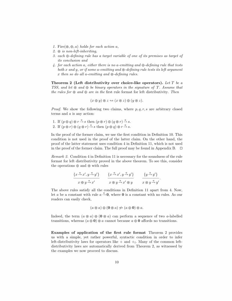
Theorem 2 (Left distributivity over choice-like operators). Let T be aTSS, and let � and � be binary operators in the signature of T . Assume thatthe rules for � and � are in the first rule format for left distributivity. Then
(x� y)� z ↔–– (x� z)� (y � z).
Proof. We show the following two claims, where p, q, r, s are arbitrary closedterms and a is any action:
1. If (p� q)� ra→ s then (p� r)� (q � r) a→ s.
2. If (p� r)� (q � r) a→ s then (p� q)� ra→ s.
In the proof of the former claim, we use the first condition in Definition 10. Thiscondition is not used in the proof of the latter claim. On the other hand, theproof of the latter statement uses condition 4 in Definition 11, which is not usedin the proof of the former claim. The full proof may be found in Appendix B. ut
Remark 2. Condition 4 in Definition 11 is necessary for the soundness of the ruleformat for left distributivity proved in the above theorem. To see this, considerthe operations � and � with rules
{x a→x′, ya→ y′}
x� ya→x′
{x a→x′, ya→ y′}
x� ya→x′ � y
{y a→ y′}
x� ya→ y′
.
The above rules satisfy all the conditions in Definition 11 apart from 4. Now,let a be a constant with rule a a→0, where 0 is a constant with no rules. As ourreaders can easily check,
(a� a)� (0� a) 6↔–– (a� 0)� a.
Indeed, the term (a � a) � (0 � a) can perform a sequence of two a-labelledtransitions, whereas (a� 0) � a cannot because a� 0 affords no transitions.
Examples of application of the first rule format Theorem 2 providesus with a simple, yet rather powerful, syntactic condition in order to inferleft-distributivity laws for operators like + and +l. Many of the common left-distributivity laws are automatically derived from Theorem 2, as witnessed bythe examples we now proceed to discuss.
10

Example 3 (Left merge and interleaving parallel composition). The operationalsemantics of the classic left-merge and interleaving parallel composition opera-tors [12, 16, 17, 23] is given by the rules below.
xa→x′
x‖ y a→x′ ‖ y
xa→x′
x ‖ y a→x′ ‖ y
ya→ y′
x ‖ y a→x ‖ y′
Note that the rules for the left-merge operator ‖ and those for any of +, +l and+r satisfy the constraints of the first rule format for left distributivity. Therefore,Theorem 2 yields the validity of the following laws.
(x+ y)‖ z ↔–– (x‖ z) + (y‖ z)(x+l y)‖ z ↔–– (x‖ z) +l (y‖ z)(x+r y)‖ z ↔–– (x‖ z) +r (y‖ z)
Observe that the equalities
(x+l y) ‖ z ↔–– (x ‖ z) +l (y ‖ z) and(x+r y) ‖ z ↔–– (x ‖ z) +r (y ‖ z)
are sound. However, their soundness cannot be shown using Theorem 2, sincethe parallel composition operator ‖ does not satisfy condition 2 in Definition 11.Indeed, x occurs in the target of the conclusion of the second rule for ‖.
Example 4 (Synchronous parallel composition). Consider the synchronous par-allel composition from CSP [22, 21]4 specified by the rules below, where a rangesover the set of actions:
xa→x′ y
a→ y′
x ‖s ya→x′ ‖s y′
.
Note that the rules for the synchronous parallel composition operator and thosefor any of +, +l and +r satisfy the constraints of the first rule format for leftdistributivity. Therefore, Theorem 2 yields the validity of the following laws.
(x+ y) ‖s z ↔–– (x ‖s z) + (y ‖s z)(x+l y) ‖s z ↔–– (x ‖s z) +l (y ‖s z)(x+r y) ‖s z ↔–– (x ‖s z) +r (y ‖s z)
Example 5 (Join and ‘/’ operators). Consider the join operator on from [15] andthe ‘hourglass’ operator / from [2] specified by the rules below, where a, b rangeover the set of actions:
xa→x′ y
a→ y′
x on ya→x′ ∓ y′
xa→x′ y
b→ y′
x/ya→x′/y′
,
4 In [22], Hoare uses the symbol ‖ to denote the synchronous parallel compositionoperator. Here we use that symbol for parallel composition.
11

where ∓ denotes the delayed choice operator from [15]. (The operational spec-ification of the delayed choice operator is immaterial for the analysis of thisexample.) The above rules and those for any of +, +l and +r satisfy the con-straints of the first rule format for left distributivity. Therefore, Theorem 2 yieldsthe validity of the following laws, where � ∈ {on, /}.
(x+ y)� z ↔–– (x� z) + (y � z)(x+l y)� z ↔–– (x� z) +l (y � z)(x+r y)� z ↔–– (x� z) +r (y � z)
Example 6 (Disrupt). Consider the following disrupt operator I [13, 18] withrules
xa→x′
xI ya→x′ I y
ya→ y′
xI ya→ y′
.
The above rules and those for any of +, +l and +r satisfy the constraints of thefirst rule format for left distributivity. Therefore, Theorem 2 yields the validityof the following laws.
(x+ y)I z ↔–– (xI z) + (y I z)(x+l y)I z ↔–– (xI z) +l (y I z)(x+r y)I z ↔–– (xI z) +r (y I z)
Example 7 (Unless operator). The unless operator / from [14] and the operator∆ from [2, page 23] are specified by the rules
xa→x′ y
b9 for a < b
x / ya→x′
xa→x′ y
b9 for a < b
x ∆ ya→ θ(x′)
,
where < is an irreflexive partial order over the set of actions and θ denotesthe priority operator from [14]. (The operational specification of the priorityoperator is immaterial for the analysis of this example.) The above rules andthose for any of +, +l and +r satisfy the constraints of the first rule format forleft distributivity. Therefore, Theorem 2 yields the validity of the following laws,where � ∈ {/,∆}.
(x+ y)� z ↔–– (x� z) + (y � z)(x+l y)� z ↔–– (x� z) +l (y � z)(x+r y)� z ↔–– (x� z) +r (y � z)
Example 8 (Interplay between the choice operators). Consider the choice opera-tors +, +l and +r from Example 1. The rules for any of the nine combinationsof those operators satisfy the constraints of the first rule format for left dis-tributivity. Therefore, Theorem 2 yields the validity of the following law, where�,� ∈ {+,+l,+r}.
(x� y)� z ↔–– (x� z)� (y � z)
12

For example, as an instance of that family of equalities, we obtain the following‘self left-distributivity law’ for any � ∈ {+,+l,+r}:
(x� y)� z ↔–– (x� z)� (y � z).
As we will see in Section 6, our first rule format for left distributivity canalso be used to derive left-distributivity laws involving unary � operators.
3.3 The second left-distributivity format
As witnessed by the above-mentioned examples, the rule format introduced inDefinition 11 can handle many of the common left-distributivity laws from theliterature. However, as we mentioned in Example 3, that rule format is notgeneral enough to prove the validity of, e.g., the left-distributivity law
(x+l y) ‖ z ↔–– (x ‖ z) +l (y ‖ z).
It is instructive to see why the equality
(p+l q) ‖ r ↔–– (p ‖ r) +l (q ‖ r)
holds for all p, q, r. The terms that can be reached from (p +l q) ‖ r via ana-labelled transition have one of the two following forms:
– p′ ‖ r, for some p′ such that p a→ p′ or– (p+l q) ‖ r′, for some r′ such that r a→ r′.
On the other hand, the terms that can be reached from (p ‖ r) +l (q ‖ r) via ana-labelled transition are of the form
– p′ ‖ r, for some p′ such that p a→ p′ or– p ‖ r′, for some r′ such that r a→ r′.
The first of those possible forms is identical to the first form of a possible deriva-tive of (p+l q) ‖ r. However, the second form—viz. p ‖ r′, for some r′ such thatra→ r′—matches (p+l q) ‖ r′ only up to one application of the equation
x+l y = x,
which is sound modulo bisimilarity, from left to right. This rewriting can beperformed in the context of ‖ since the rules for the interleaving parallel compo-sition operator given in Example 3 are in de Simone format [20], which is one ofthe congruence formats for bisimilarity—see, for instance, the survey articles [9,27].
The above discussion motivates the development of a generalization of therule format we presented in Definition 11. The main idea behind this more power-ful rule format is to weaken the constraints for ensuring the ‘matching-conclusioncondition’, so that terms that are targets of transitions from (p � q) � r and
13

(p � r) � (q � r) need only be equal up to the application of some equation,whose validity modulo bisimilarity can be justified ‘syntactically’, in a contextconsisting of operations that preserve bisimilarity. Of course, the resulting defi-nition of the rule format depends on the set of equations that one is allowed touse. Indeed, one can obtain more powerful rule formats by simply extending thecollection of allowed equations. Therefore, what we now present can be seen as atemplate for rule formats guaranteeing the validity of left-distributivity equationsof the form (1). Our definition of the second rule format is based on a rewritingrelation over terms that is sufficient to handle the examples from the literaturewe have met so far. The rewriting relation we present below can, however, beeasily strengthened by adding more rewritings, provided their soundness withrespect to bisimilarity can be ‘justified syntactically’. (See the paragraphs afterDefinition 12 and Remark 4 for a brief discussion of extensions of the proposedrule format.)
Definition 12 (The rewriting relation ) Let T = (Σ,L, D) be a TSS.
1. The relation is the least binary relation over T(Σ) that satisfies the fol-lowing clauses, where we use t! t′ as a short-hand for t t′ and t′ t:– t t,– f(t, t)! t, if T is in idempotence format with respect to f from [1],– C[t] C[t′], if t t′ and T is in a congruence format for ↔––,– t1 +l t2 t1, if +l ∈ Σ,– t1 +r t2 t2, if +r ∈ Σ, and
2. Let � and � be two binary operations in Σ. We write t↓�,�u if, and only, ifthere are some t′ and u′ such that t t′, u u′, and t′ = u′ can be provedby possibly using one application of axiom
(x� y) � z = (x� z)� (y � z)
at the top level—that is, either t′ ≡ u′ or t′ ≡ (t1 � t2) � t3 and u′ =(t1 � t3)� (t2 � t3), for some t1, t2, t3.
Lemma 1. Let T = (Σ,L, D) be a TSS. If t t′ then t ↔–– t′, for all t, t′ ∈T(Σ).
Proof. By induction on the definition of . The soundness of the rewrite rules
– f(t, t)! t, if T is in idempotence format with respect to f from [1], and– C[t] C[t′], if t t′ and T is in a congruence format for ↔––,
is guaranteed by results in [1] and in the classic theory of structural operationalsemantics. ut
In order to check whether a rewriting rule preserves bisimilarity, in all casesapart from the the first, the above definition relies on existing rule formatsguaranteeing the validity of algebraic laws modulo bisimilarity, see [11], or onequations whose soundness with respect to bisimilarity is easy to check, such as
x+l y = x and x+r y = y.
14

This choice allows us to achieve an expressive and extensible rule format whileretaining its syntactic nature. For instance, one may easily extend the rewritingrelation with the following two clauses:
– f(t1, t2) ! f(t2, t1), if T is in the commutativity rule format with respectto f from [26], and
– f(t, f(t′, t′′)) ! f(f(t, t′), t′′), if T is in the associativity rule format withrespect to f from [19].
While proving the soundness of a left-distributivity law of the form
(x� y)� z ↔–– (x� z)� (y � z),
the validity of equivalences of the form
(t� t′) � t′′ = (t� t′′) � (t′ � t′′)
will be guaranteed by coinduction.In Definition 13 to follow, which is the key ingredient in the definition of our
second rule format for left distributivity, we shall use the relation ↓�,� to describewhen a �-defining rule d1 is ‘distributivity compliant’ to a �-defining rule d2.The intuitive idea is that this will hold when those two rules can be combinedto derive transitions from terms of the form (p� q)� r and (p� r)� (q� r) that‘match’ up to bisimilarity. Since the definition of distributivity compliance isquite technical, we find it useful to explain, by means of examples, the intuitionbehind it. For the sake of consistency and clarity, in the examples to follow, weshall use the same naming convention for substitutions that will be employed inDefinition 13.
Suppose that the transition (p� q) � ra→ s is proved using rule d1 and rule
d2. Assume, furthermore, that
(d1){x a→x′, y
a→ y1, yb→ y2}
x� ya→ t
and that d2 tests only one of its arguments, say
(d2){x a→x′}x� y
a→ t′.
Then s = σ1(t), where
σ1 = [x 7→ p� q, y 7→ r, x′ 7→ σ′2(t′), y1 7→ r1, y2 7→ r2]σ′2 = [x 7→ p, y 7→ q, x′ 7→ p′]
and pa→ p′, r a→ r1 and r
b→ r2.As highlighted by the proof of Theorem 1, rules d2 and d1 can be used to
derive a transition (p� r) � (q � r) a→σ2(t′), where
σ2 = [x 7→ p� r, y 7→ q � r, x′ 7→ σ1x(t)]σ1x = [x 7→ p, y 7→ r, x′ 7→ p′, y1 7→ r1, y2 7→ r2].
15
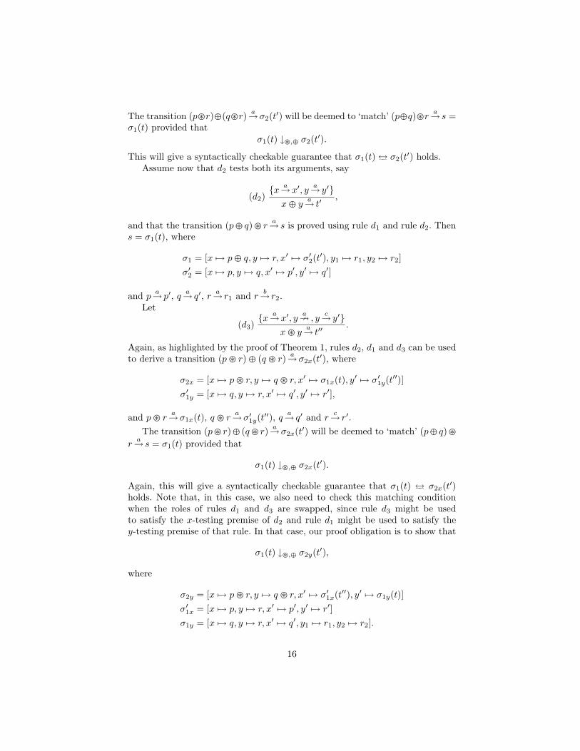
The transition (p�r)�(q�r) a→σ2(t′) will be deemed to ‘match’ (p�q)�r a→ s =σ1(t) provided that
σ1(t) ↓�,� σ2(t′).
This will give a syntactically checkable guarantee that σ1(t)↔–– σ2(t′) holds.Assume now that d2 tests both its arguments, say
(d2){x a→x′, y
a→ y′}x� y
a→ t′,
and that the transition (p� q)� r a→ s is proved using rule d1 and rule d2. Thens = σ1(t), where
σ1 = [x 7→ p� q, y 7→ r, x′ 7→ σ′2(t′), y1 7→ r1, y2 7→ r2]σ′2 = [x 7→ p, y 7→ q, x′ 7→ p′, y′ 7→ q′]
and pa→ p′, q a→ q′, r a→ r1 and r
b→ r2.Let
(d3){x a→x′, y
a9 , yc→ y′}
x� ya→ t′′
.
Again, as highlighted by the proof of Theorem 1, rules d2, d1 and d3 can be usedto derive a transition (p� r)� (q � r) a→σ2x(t′), where
σ2x = [x 7→ p� r, y 7→ q � r, x′ 7→ σ1x(t), y′ 7→ σ′1y(t′′)]σ′1y = [x 7→ q, y 7→ r, x′ 7→ q′, y′ 7→ r′],
and p� ra→σ1x(t), q � r
a→σ′1y(t′′), q a→ q′ and rc→ r′.
The transition (p� r)� (q� r) a→σ2x(t′) will be deemed to ‘match’ (p� q)�ra→ s = σ1(t) provided that
σ1(t) ↓�,� σ2x(t′).
Again, this will give a syntactically checkable guarantee that σ1(t) ↔–– σ2x(t′)holds. Note that, in this case, we also need to check this matching conditionwhen the roles of rules d1 and d3 are swapped, since rule d3 might be usedto satisfy the x-testing premise of d2 and rule d1 might be used to satisfy they-testing premise of that rule. In that case, our proof obligation is to show that
σ1(t) ↓�,� σ2y(t′),
where
σ2y = [x 7→ p� r, y 7→ q � r, x′ 7→ σ′1x(t′′), y′ 7→ σ1y(t)]σ′1x = [x 7→ p, y 7→ r, x′ 7→ p′, y′ 7→ r′]σ1y = [x 7→ q, y 7→ r, x′ 7→ q′, y1 7→ r1, y2 7→ r2].
16

Definition 13 (Distributivity compliance up to ) Let T be a TSS, andlet � and � be binary operators in the signature of T . Let d1 be a �-definingrule in T and d2 be a �-defining rule in T . We say that d1 is distributivitycompliant to d2 up to , and we write it d1
∼ d2, whenever
1. rule d1 is of the form (R1) and rule d2 is of the form (R2),2. the collection of positive y-testing premises in d1 is of the form {y ai→ yi | i ∈
I}, for some index set I, where all the variables are pairwise distinct, and3. one of the following two cases applies:
(a) d2 has premises {x a→x′} or {y a→ y′}, and
σ1(toc(d1)) ↓�,� σ2(toc(d2)),
or(b) d2 has premises {x a→x′, y
a→ y′} and, for each rule d3 ∈ D(�, a),– the collection of positive y-testing premises in d3 is of the form{y aj→ yj | j ∈ J}, for some index set J , where all the variables arepairwise distinct,
– σ1(toc(d1)) ↓�,� σ2x(toc(d2)) and– σ1(toc(d1)) ↓�,� σ2y(toc(d2)),
where the substitutions σ1, σ1x, σ1y, σ2, σ2x and σ2y are defined as follows,with p, q, p′, q′, r, r′, and all the variables in {ri | i ∈ I}∪{rj | j ∈ J} beingfresh and pairwise distinct variables.– σ1 = [x 7→ p� q, y 7→ r, x′ 7→ σ′2(toc(d2)), yi 7→ ri (i ∈ I)].– σ2 = [x 7→ p� r, y 7→ q � r, x′ 7→ σ1x(toc(d1)), y′ 7→ σ1y(toc(d1))].– σ′2 = [x 7→ p, y 7→ q, x′ 7→ p′, y′ 7→ q′].– σ1x = [x 7→ p, y 7→ r, x′ 7→ p′, yi 7→ ri (i ∈ I)].– σ′1x = [x 7→ p, y 7→ r, x′ 7→ p′, yj 7→ rj (j ∈ J)].– σ1y = [x 7→ q, y 7→ r, x′ 7→ q′, yi 7→ ri (i ∈ I)].– σ′1y = [x 7→ q, y 7→ r, x′ 7→ q′, yj 7→ rj (j ∈ J)].– σ2x = [x 7→ p� r, y 7→ q � r, x′ 7→ σ1x(toc(d1)), y′ 7→ σ′1y(toc(d3))].– σ2y = [x 7→ p� r, y 7→ q � r, x′ 7→ σ′1x(toc(d3)), y′ 7→ σ1y(toc(d1))].
The reader should notice that, in order not to complicate the definition fur-ther by a more refined case distinction, in condition 3a of Definition 13, thesubstitution σ2 is defined for both x′ and y′, even if in that case only one ofthem appears in rule d2.
The following result is straightforward.
Theorem 3 (Decidability of ∼). Let T be a TSS, and let � and � be binaryoperators in the signature of T . Let d1 be a �-defining rule in T and d2 bea �-defining rule in T . The problem of determining whether d1
∼ d2 holds isdecidable.
Remark 3. Note that ∼ performs only one rewriting step on both the terms.Clearly, extending Definition 13 in order to consider any finite amount of rewrit-ing steps would not jeopardize Theorem 3.
17

We now have all the necessary ingredients to define our second rule formatfor left distributivity.
Definition 14 (Second left-distributivity format) A TSS T is in the sec-ond left-distributivity format for a binary operator � with respect to a binaryoperator � whenever, for each action a,
1. Fire(�,�, a), and2. if D(�, a) 6= ∅ then d1
∼d2, for each d1 ∈ D(�, a) and for each d2 ∈ D(�, a).
We are now ready to formulate the two main theorems of the paper.
Theorem 4 (Soundness of the second left-distributivity format). Let Tbe a TSS. If T is in the second left-distributivity format for � with respect to �then
(x� y) � z ↔–– (x� z)� (y � z).
Proof. A proof of this result may be found in Appendix C. ut
Remark 4. The above theorem holds true for any notion of distributivity com-pliance up to rewriting that is based on a rewriting relation over terms thathas the following properties:
– ⊆↔–– and– is decidable.
The latter requirement is not necessary for the soundness of the format. However,it is highly desirable from the point of view of applications. Indeed, in order toobtain a bona fide rule format, the relation should be defined by using ruleswhose applicability can be checked syntactically, for instance using extant ruleformat for operational semantics. The proposal we presented in Definition 12 fitsthis requirement.
The following result is straightforward, but important from the point of viewof applications. In its statement, we use Range(f) to stand for the set of actionsa for which there exists an a-emitting f -defining rule.
Theorem 5 (Decidability of the second rule format). Let T be a TSS,and let � and � be two binary operators from the signature of T . Assume thatRange(�) is finite, and that D(�, a)∪D(�, a) is finite for each a ∈ Range(�).Then it is decidable whether T is in the second left-distributivity format for �with respect to �.
The import of Theorems 4 and 5 is that, when establishing that an operator� is left distributive with respect to an operator �, it is sufficient to checkwhether the SOS specification for those operators meets the conditions of theformat of Definition 14, which can be done effectively when the TSS under studyis finite.
18

4 Analyzing the distributivity compliance
In this section, we reduce the analysis of distributive compliance ∼ to a syntac-tic check on the targets of the conclusions of the �- and �-defining rules. Byanalyzing different possible syntactic shapes for terms, we check which pairs ofshapes can be related using the distributivity-compliance relation. This analysisis useful in order to avoid many of the substitutions involved in Definition 13,and, as witnessed by some of the examples in Section 5, to avoid all of them inmany cases.
Table 1 summarizes our results. Even though the offered list is not exhaustive,which, at first sight, seems a challenging task to achieve, we believe Table 1 offersenough cases to avoid substitutions completely in most cases.
Table 1. Analysis of the distributivity-compliance pairs
toc(d1) toc(d2) result further requirements
1 x′ � y x p� r
2 x′ � y y q � r
3 x x′ � y′ p� q D(�, a) = {d1}4 x′ x′ � y′ p′ � q′ D(�, a) = {d1}5 x� t x′ � y′ (p� q) � σ(t) D(�, a) = {d1}, x, x′ 6∈ vars(t)
6 x′ � t x′ � y′ (p′ � q′) � σ(t) D(�, a) = {d1}, x, x′ 6∈ vars(t)
7 t x′ � y′ σ(t) � idempotent, D(�, a) = {d1}, x, x′ 6∈ vars(t)
8 t x′ σ′(t) Condition 4 of Definition 11, x 6∈ vars(t)
9 t y′ σ′(t) Condition 4 of Definition 11, x 6∈ vars(t)
with σ = [y 7→ r, yi 7→ ri (i ∈ I)] and σ′ = [y 7→ r, x′ 7→ p′, yi 7→ ri (i ∈ I)]
In Table 1, x and y are considered as the variables for the first and secondargument, respectively, for both �- and �-defining rules. When the variable x′
is mentioned, implicitly the considered rule has a premise x a→x′ (for a-emittingrules). Similarly, when the variable y′ is mentioned, implicitly the rule consid-ered has a premise y a→ y′. The term t stands for a generic open term from thesignature, and, following Definition 13, p, q and r are hypothetical closed termsapplied to the distributivity equation in this way: (p� q)� r ↔–– (p� r)� (q� r).The symbols p′, q′, and ri, are considered as targets of possible transitions pos-sible transitions from p, q and r.
Table 1 is to be read as follows. First of all, d1 ∈ D(�, a) and d2 ∈ D(�, a),for some action a. In each row, the first column (column toc(d1)) specifies theform of the target of the conclusion of the �-defining rule d1 (e.g., x in case ofrow 3), and the second column (column toc(d2)) specifies the form of the targetof the conclusion of the �-defining rule d2 (e.g., x′ � y′ in case of row 3). If theconditions in the column further requirements are satisfied (e.g., in row 3, d1
is the only �-defining and a-emitting rule), then the result of the transition of
19

terms (p�q)�r and (p�r)�(q�r) is specified by the term given in column result(e.g., p�q in row 3). In rows 5–6, the stated result is up to one application of theleft-distributivity equation (1). The requirement � idempotent means that theoperator � can be proved idempotent, e.g., by means of the rule format offeredin [1].
The reader may want to notice that the first rule format of Section 3.2 ispartly based on the analysis which leads to rows 8 and 9.
Theorem 6 (Soundness of Table 1). Let T be a TSS. Let � and � be binaryoperations in the signature of T satisfying
1. Fire(�,�, a), and2. if D(�, a) 6= ∅ then for each d1 ∈ D(�, a) and for each d2 ∈ D(�, a), the
rules d1 and d2 match a row in Table 1.
It holds that:(x� y) � z ↔–– (x� z)� (y � z).
Proof. The proof of the theorem goes by a straightforward check of the conditionsof Definition 13 on the combination specified in each row. For example, we discussthe case of row 7 in some detail below.
Applying the substitutions, we can see that on the left side of the distribu-tivity equation (p � q) � r ↔–– (p � r) � (q � r), we can prove the transition(p � q) � r
a→ v, with v = t[x 7→ p � q, y 7→ r, x′ 7→ (x′ � y′)[x 7→ p, y 7→ q,x′ 7→ p′, y′ 7→ q′], yi 7→ ri (i ∈ I)], and thus
v = t[x 7→ p� q, y 7→ r, x′ 7→ p′ � q′, yi 7→ ri (i ∈ I)].
On the right side of the distributivity equation, we can prove the transition(p � r) � (q � r) a→ v′, with v′ = (x′ � y′)[x 7→ p � r, y 7→ q � r, x′ 7→ t[x 7→ p,y 7→ r, x′ 7→ p′, yi 7→ ri (i ∈ I)]), y′ 7→ t[x 7→ q, y 7→ r, x′ 7→ q′, yi 7→ ri (i ∈ I)],and thus v′ = v′1 � v′2, where
v′1 = t[x 7→ p, y 7→ r, x′ 7→ p′, yi 7→ ri (i ∈ I)] andv′2 = t[x 7→ q, y 7→ r, x′ 7→ q′, yi 7→ ri (i ∈ I)].
From the column further requirements of row 7, we know that the variables x andx′ do not appear in t, leading the two terms to be v = t[y 7→ r, yi 7→ ri (i ∈ I)]and v′ = v � v. Since, as a further requirement, the operator � is idempotentwith respect to bisimilarity, i.e., x� x↔–– x, we can conclude that
v′ ↓�,� v = t[y 7→ r, yi 7→ ri (i ∈ I)],
where t[y 7→ r, yi 7→ ri (i ∈ I)] is the term stated in the column result of row7. ut
20
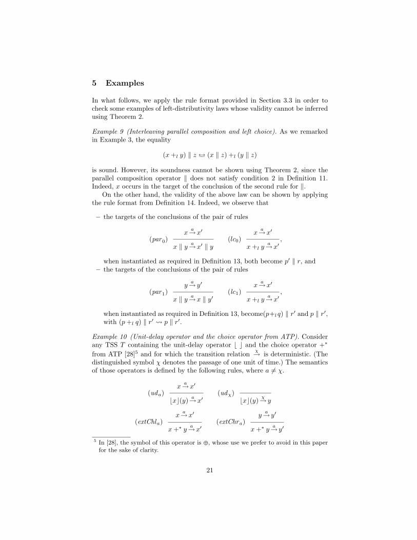
5 Examples
In what follows, we apply the rule format provided in Section 3.3 in order tocheck some examples of left-distributivity laws whose validity cannot be inferredusing Theorem 2.
Example 9 (Interleaving parallel composition and left choice). As we remarkedin Example 3, the equality
(x+l y) ‖ z ↔–– (x ‖ z) +l (y ‖ z)
is sound. However, its soundness cannot be shown using Theorem 2, since theparallel composition operator ‖ does not satisfy condition 2 in Definition 11.Indeed, x occurs in the target of the conclusion of the second rule for ‖.
On the other hand, the validity of the above law can be shown by applyingthe rule format from Definition 14. Indeed, we observe that
– the targets of the conclusions of the pair of rules
(par0)xa→x′
x ‖ y a→x′ ‖ y(lc0)
xa→x′
x+l ya→x′
,
when instantiated as required in Definition 13, both become p′ ‖ r, and– the targets of the conclusions of the pair of rules
(par1)ya→ y′
x ‖ y a→x ‖ y′(lc1)
xa→x′
x+l ya→x′
,
when instantiated as required in Definition 13, become(p+lq) ‖ r′ and p ‖ r′,with (p+l q) ‖ r′ p ‖ r′.
Example 10 (Unit-delay operator and the choice operator from ATP). Considerany TSS T containing the unit-delay operator b c and the choice operator +∗
from ATP [28]5 and for which the transition relationχ→ is deterministic. (The
distinguished symbol χ denotes the passage of one unit of time.) The semanticsof those operators is defined by the following rules, where a 6= χ.
(uda)xa→x′
bxc(y) a→x′(udχ)
bxc(y)χ→ y
(extChla)xa→x′
x+∗ y a→x′(extChra)
ya→ y′
x+∗ y a→ y′
5 In [28], the symbol of this operator is �, whose use we prefer to avoid in this paperfor the sake of clarity.
21

(extTime)xχ→x′ y
χ→ y′
x+∗ yχ→x′ +∗ y′
We claim that T is in the second left-distributivity format for b c with respectto +∗. Indeed, we observe that
– the targets of the conclusions of the pair of rules (uda, extChla) when in-stantiated as required in Definition 13, both become p′,
– the targets of the conclusions of the pair of rules (uda, extChra) when in-stantiated as required in Definition 13, both become q′, and
– the targets of the conclusions of the pair of rules (udχ, extT ime) when in-stantiated as required in Definition 13, become r and r+∗ r, with r+∗ r rbecause T is in idempotence format with respect to +∗, as argued in [1,Example 9].
The well-known law
bx+∗ yc(z)↔–– bxc(z) +∗ byc(z)
thus follows from Theorem 4.Table 1 can be used to match the targets of the conclusions as follows: the
combination of uda and extChla follows from row 8, the combination of uda andextChra follows from row 9, and finally the combination of udχ and extTimefollows from row 7.
Example 11 (Timed left merge and the choice operator from ATP). Consider theTSS for ATP with the timed extension of the left-merge operator from Example 3specified by the following rules, where a 6= χ:
(mergea)xa→x′
x‖ y a→x′ ‖ y(mergeχ)
xχ→x′ y
χ→ y′
x‖ y χ→x′‖ y′.
We claim that this TSS is in the second left-distributivity format for ‖ withrespect to +∗. We limit ourselves to checking that the targets of the conclusionsof the second rule for ‖ and rule extT ime match when instantiated as requiredin Definition 13. This follows because, in all cases, the resulting terms yield aninstance of the equality
(p′ +∗ q′)‖ r′ = (p′‖ r′) +∗ (q′‖ r′).
The law(x+∗ y)‖ z = (x‖ z) +∗ (y‖ z)
thus follows from Theorem 4.Checking the conditions of the second rule format can be simplified by using
the syntactic checks of Table 1, as follows: the combination mergea, extChlafollows from row 8, the combination mergea, extChra follows from row 9 and thecombination mergeχ, extTime follows from row 6.
22

6 Examples of left-distributivity laws involving unaryoperators
In this section we apply the rule formats from Section 3 in order to prove left-distributivity laws involving unary operators from the literature. In order to doso, we turn unary operators into binary operators that simply ignore their rightargument.
We begin with three examples that can be dealt with using Theorem 2.
Example 12 (Encapsulation and choice). Consider the classic unary encapsula-tion operators ∂H from ACP [12], where H ⊆ L, with rules
xa→x′
∂H(x) a→ ∂H(x′)a 6∈ H.
It is well known that
∂H(x+ y)↔–– ∂H(x) + ∂H(y), (2)
where + is the choice operator from Example 1.We shall now argue that the validity of this equation can be shown using The-
orem 2. To this end, we turn the encapsulation operators into binary operatorsthat ignore their second argument. The above rules therefore become
xa→x′
∂H(x, y) a→ ∂H(x′, y)a 6∈ H.
Note that the rules for ∂H and + are in the first rule format for left distributivityfrom Definition 11. In particular, Fire(∂H ,+, a) holds for each action a, becauseif there is an a-emitting rule for ∂H then there is also an a-emitting rule for+. (Note that the converse only holds if H = ∅. This explains the asymmetricnature of the constraint Fire(�,�, a).) Therefore Theorem 2 yields the validityof the left-distributivity law
∂H(x+ y, z)↔–– ∂H(x, z) + ∂H(y, z),
from which the soundness of (2) follows immediately.
Example 13 (Match operator and choice). Consider the unary match operators[a = b] from the π-calculus [33]6, where a, b ∈ L, with rules
xc→x′
[a = b](x) c→x′if a = b,
where c ∈ L.6 Note that in the π-calculus a and b in the formula [a = b]p are names and not labels.
23

It is well known that
[a = b](x+ y)↔–– [a = b](x) + [a = b](y), (3)
where + is the choice operator from Example 1.We shall now argue that the validity of this equation can be shown using
Theorem 2. To this end, as above, we turn the match operators into binaryoperators that ignore their second argument. The above rules therefore become
xc→x′
[a = b](x, y) c→x′if a = b.
Note that the rules for [a = b] and + are in the first rule format for left dis-tributivity from Definition 11. Therefore Theorem 2 yields the validity of theleft-distributivity law
[a = b](x+ y, z)↔–– [a = b](x, z) + [a = b](y, z),
from which the soundness of (3) follows immediately.
Example 14 (Projection operator and choice). Consider the unary projection op-erators πn from ACP [12, 16], where n ≥ 0, with rules
xa→x′
πn+1(x) a→πn(x′)a ∈ L.
It is well known thatπn(x+ y)↔–– πn(x) + πn(y), (4)
where + is the choice operator from Example 1.We shall now argue that the validity of this equation can be shown using
Theorem 2. Again, we turn the projection operators into binary operators thatignore their second argument. The above rules therefore become
xa→x′
πn+1(x, y) a→πn(x′, y)a ∈ L.
Note that the rules for πn and + are in the first rule format for left distribu-tivity from Definition 11. Therefore Theorem 2 yields the validity of the left-distributivity law
πn(x+ y, z)↔–– πn(x, z) + πn(y, z),
from which the soundness of (4) follows immediately.
Example 15 (Prefix operator and synchronous parallel operator). Consider anyTSS T containing the synchronous parallel operator ‖s from Example 4 andcontaining the following binary version of the prefix operator from CCS [23],where a ranges over a set of actions L:
24

prefa =a.(x, y) a→x
.
We claim that T is in the second left-distributivity format for the prefixoperator with respect to ‖s. Let us pick an action a. Then the targets of theconclusions of prefa and of
xa→x′ y
a→ y′
x ‖s ya→x′ ‖s y′
,
which is the only a-emitting rule for ‖s, both yield the term p ‖s q when instan-tiated as required in Definition 13. Therefore, Theorem 4 yields the validity ofthe law
a.(x ‖s y, z)↔–– a.(x, z) ‖s a.(y, z).
Turning the prefix operator back to its unary version, we obtain the soundnessof the following equality:
a.(x ‖s y)↔–– a.x ‖s a.y.
Row 3 in Table 1 can be used to match the targets of the conclusions of thesynchronous parallel composition and the prefix operators.
Example 16 (Unit-delay operator and choice operator). Consider any TSS T thatincludes the choice operator +∗ from Example 10 and the following binary ver-sions of the unit-delay operator:
delay1 =(1)(x, y)
χ→x.
We claim that T is in the second left-distributivity format for (1) with respectto +∗. To see this, it suffices to observe that the targets of the conclusions ofthe χ-emitting rules for those two operators, when instantiated as required inDefinition 13, both yield the term p+∗q. Therefore, Theorem 4 yields the validityof the law
(1)(x+∗ y, z)↔–– (1)(x, z) +∗ (1)(y, z).
Turning the unit-delay operator back to its unary version, we obtain the well-known law
(1)(x+∗ y)↔–– (1)(x) +∗ (1)(y).
Row 3 in Table 1 can be used to match the targets of the conclusions of thedelay rules for the unit-delay and choice operators.
25

7 Impossibility results
In this section we provide some impossibility results concerning the validity of theleft-distributivity law. Unlike previous results about rule formats for algebraicproperties, such as those surveyed in [11], we offer theorems to recognize whenthe left-distributivity law is guaranteed not to hold. When designing operationalspecifications for operators that are intended to satisfy a left-distributivity law,a language designer might also benefit from considering these kinds of negativeresults.
7.1 Left-inheriting operators
Our first negative result will concern a kind of left-inheriting operator, which wecall strong left-inheriting and we now proceed to define.
Definition 15 (Forwarder operators) Let−→k = (k1, k2, . . . , k`), where 1 ≤
` ≤ n and 1 ≤ k1 < k2 < . . . < k` ≤ n. An operator f of arity n is a−→k -
forwarder if the following conditions hold for each action a and for all closedterms p1, . . . , pn:
– if f(p1 . . . , pk1 , . . . , pk2 , . . . , pk`, . . . , pn) a→ then there is some 1 ≤ i ≤ ` such
that pki
a→ and– for each 1 ≤ i ≤ `, if pki
a→ then f(p1 . . . , pk1 , . . . , pk2 , . . . , pk`, . . . , pn) a→ .
Syntactic conditions to guarantee that an operator is a−→k -forwarder can be
given. However, this is beyond the scope of the present paper.
Example 17. As the reader can easily check, the left-merge operator ‖ from Ex-ample 3 and the replication operator ! given by the rules below
xa→x′
!x a→x′ ‖!x(a ∈ L),
where ‖ is the interleaving parallel composition operator from Example 3, are(1)-forwarders. On the other hand, the interleaving parallel composition operatorand the choice operator + from Example 1 are (1, 2)-forwarders.
Definition 16 (Forwarder contexts) The grammar for forwarder contextsfor a variable x is
F [x] ::= x | f(x1, . . . , xi−1, F [x], xi+1, . . . , xn),
where f is an n-ary operator, x1, . . . , xi−1, xi+1, . . . , xn are variables, F [x] ap-pears as the ith argument of f , and f is
−→k -forwarder with i appearing in
−→k .
Lemma 2. Assume that F [x] is a forwarder context for a variable x. Then, foreach closed substitution σ and for each action a, the following statements hold:
26
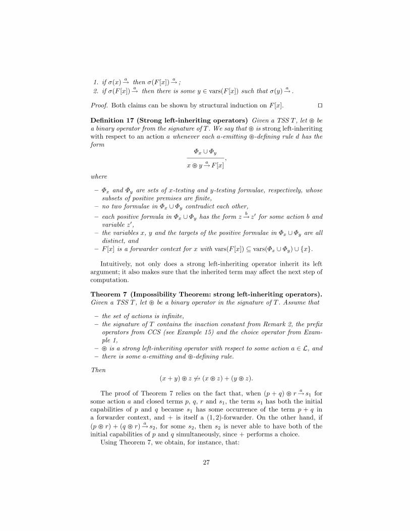
1. if σ(x) a→ then σ(F [x]) a→ ;2. if σ(F [x]) a→ then there is some y ∈ vars(F [x]) such that σ(y) a→ .
Proof. Both claims can be shown by structural induction on F [x]. ut
Definition 17 (Strong left-inheriting operators) Given a TSS T , let � bea binary operator from the signature of T . We say that � is strong left-inheritingwith respect to an action a whenever each a-emitting �-defining rule d has theform
Φx ∪ Φy
x� ya→F [x]
,
where
– Φx and Φy are sets of x-testing and y-testing formulae, respectively, whosesubsets of positive premises are finite,
– no two formulae in Φx ∪ Φy contradict each other,
– each positive formula in Φx ∪ Φy has the form zb→ z′ for some action b and
variable z′,– the variables x, y and the targets of the positive formulae in Φx ∪ Φy are all
distinct, and– F [x] is a forwarder context for x with vars(F [x]) ⊆ vars(Φx ∪ Φy) ∪ {x}.
Intuitively, not only does a strong left-inheriting operator inherit its leftargument; it also makes sure that the inherited term may affect the next step ofcomputation.
Theorem 7 (Impossibility Theorem: strong left-inheriting operators).Given a TSS T , let � be a binary operator in the signature of T . Assume that
– the set of actions is infinite,– the signature of T contains the inaction constant from Remark 2, the prefix
operators from CCS (see Example 15) and the choice operator from Exam-ple 1,
– � is a strong left-inheriting operator with respect to some action a ∈ L, and– there is some a-emitting and �-defining rule.
Then(x+ y) � z 6↔–– (x� z) + (y � z).
The proof of Theorem 7 relies on the fact that, when (p + q) � ra→ s1 for
some action a and closed terms p, q, r and s1, the term s1 has both the initialcapabilities of p and q because s1 has some occurrence of the term p + q ina forwarder context, and + is itself a (1, 2)-forwarder. On the other hand, if(p � r) + (q � r) a→ s2, for some s2, then s2 is never able to have both of theinitial capabilities of p and q simultaneously, since + performs a choice.
Using Theorem 7, we obtain, for instance, that:
27

– (x+ y) ‖ z 6↔–– (x ‖ z) + (y ‖ z)– a.(x+ y) 6↔–– (a.x) + (a.y)– !(x+ y) 6↔–– (!x) + (!y)
For the last two cases, in order to apply the above-mentioned theorem, oneneeds to consider the binary version of the action prefixing operator from Ex-ample 15 and the binary version of the replication operator, which ignores itssecond argument and can be defined along the lines we followed in the examplesin Section 6.
7.2 The use of negative premises
We now present two results that rely on the use of negative premises in rules.
Definition 18 (Always Moving Operators) Given a TSS T , we say that anoperator f from the signature of T with arity n is always moving for action awhenever f(−→p ) a→ , for each n-tuple of closed terms −→p .
For example, an n-ary operator f , with n ≥ 1, is always moving for action awhen the set of rules D(f, a) contains
– either some rule d with hyps(d) = ∅,– or rules d1, d2 with hyps(d1) = {x1
a→x′1} and hyps(d2) = {x1a9 }.
An example of operator that is always moving for action a is the prefixing op-erator a. .
Remark 5. It is possible to find syntactic conditions on the set of rules for someoperator f guaranteeing that f is always moving. For instance, the decidablelogic of initial transition formulae offered in [3], which is able to reason aboutfirability of GSOS rules, can be used in order to check whether operators arealways moving. The development of rule formats for always-moving operators is,however, orthogonal to the gist of this paper and therefore we do not address ithere.
Theorem 8. Given a TSS T , let � and � be binary operators in the signatureof T . Assume that
1. the signature of T contains at least one constant,2. a ∈ L,3. � is always moving for action a, and4. the set of premises of each a-emitting and �-defining rule contains either
xa9 or y a9 .
Then(x� y) � z 6↔–– (x� z)� (y � z),
and any triple of closed terms witnesses the above inequivalence.
28
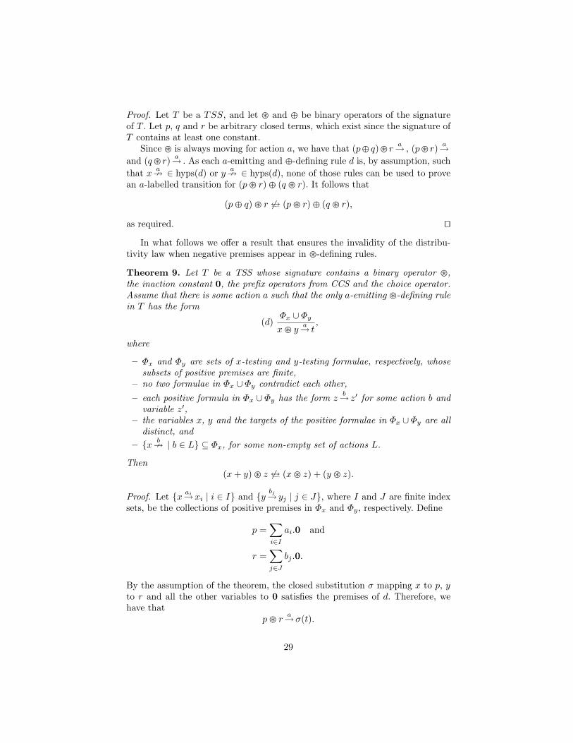
Proof. Let T be a TSS, and let � and � be binary operators of the signatureof T . Let p, q and r be arbitrary closed terms, which exist since the signature ofT contains at least one constant.
Since � is always moving for action a, we have that (p� q)� r a→ , (p� r) a→and (q� r) a→ . As each a-emitting and �-defining rule d is, by assumption, suchthat x a9 ∈ hyps(d) or y a9 ∈ hyps(d), none of those rules can be used to provean a-labelled transition for (p� r)� (q � r). It follows that
(p� q)� r 6↔–– (p� r) � (q � r),
as required. ut
In what follows we offer a result that ensures the invalidity of the distribu-tivity law when negative premises appear in �-defining rules.
Theorem 9. Let T be a TSS whose signature contains a binary operator �,the inaction constant 0, the prefix operators from CCS and the choice operator.Assume that there is some action a such that the only a-emitting �-defining rulein T has the form
(d)Φx ∪ Φyx� y
a→ t,
where
– Φx and Φy are sets of x-testing and y-testing formulae, respectively, whosesubsets of positive premises are finite,
– no two formulae in Φx ∪ Φy contradict each other,– each positive formula in Φx ∪ Φy has the form z
b→ z′ for some action b andvariable z′,
– the variables x, y and the targets of the positive formulae in Φx ∪ Φy are alldistinct, and
– {x b9 | b ∈ L} ⊆ Φx, for some non-empty set of actions L.
Then(x+ y)� z 6↔–– (x� z) + (y � z).
Proof. Let {x ai→xi | i ∈ I} and {y bj→ yj | j ∈ J}, where I and J are finite indexsets, be the collections of positive premises in Φx and Φy, respectively. Define
p =∑i∈I
ai.0 and
r =∑j∈J
bj .0.
By the assumption of the theorem, the closed substitution σ mapping x to p, yto r and all the other variables to 0 satisfies the premises of d. Therefore, wehave that
p� ra→σ(t).
29

Let q = b.0 for some b ∈ L. Then,
(p� r) + (q � r) a→σ(t).
On the other hand, the term (p+ q)� r does not afford an a-labelled transitionbecause p + q
b→0 and therefore no closed substitution mapping x to p + q cansatisfy the premises of d, which is the only a-emitting �-defining rule in T . Thismeans that
(p+ q)� r 6↔–– (p� r) + (q � r),
and the claim follows. ut
Example 18. Let > be an irreflexive partial order over L. The priority operatorΘ from [14] is specified by the following rules:
xa→x′, x
b9 (∀b > a)
Θ(x) a→Θ(x′)(a ∈ L).
The binary version of that operator can be defined following the lines presentedin the examples in Section 6. Theorem 9, when applied to the binary version ofΘ, yields the well-known fact that, when > is a non-trivial partial order,
Θ(x+ y) 6↔–– Θ(x) +Θ(y).
Indeed, if > is non-trivial, then there are actions a and b with a < b. The singlea-emitting rule for the binary version of Θ has a negative premise of the formx
b9 , and therefore Theorem 9 is applicable to derive the above inequivalence.
8 Conclusions
In this paper we have provided two rule formats guaranteeing that certain binaryoperators are left distributive with respect to choice-like operators. As witnessedby the wealth of examples we discussed in the main body of this study, the ruleformats are general enough to cover relevant examples from the literature. Inparticular, they can also be applied to establish the validity of left-distributivitylaws involving unary operators. This can be achieved by simply considering unaryoperators as binary operators that ignore their second argument.
We have also offered conditions that allow one to recognize the invalidityof the left-distributivity law in the context of left-inheriting operators and inthe presence of negative premises. Such conditions can be applied to well-knownexamples of invalid left-distributivity laws.
The research presented in this article opens several interesting lines for futureinvestigation. First of all, our rule formats can be easily adapted to obtain ruleformats guaranteeing the validity of right-distributivity laws of the form
x� (y � z) = (x� y)� (x� z).
30
The rule formats we have presented should also be extended in order to handleexamples of distributivity laws where � is not ‘choice-like’. It would also beinteresting to see whether one can relax the syntactic constraints of the ruleformats presented in this paper substantially, while preserving their soundnessand ease of application.
Last, but not least, we intend to find further ‘impossibility theorems’ alongthe lines of those we presented in Section 7.
This future work will lead to a better understanding of the semantic natureof distributivity properties and of its links to the syntax of SOS rules.
References
1. L. Aceto, A. Birgisson, A. Ingolfsdottir, M. R. Mousavi, and M. A. Reniers. Ruleformats for determinism and idempotence. In F. Arbab and M. Sirjani, edi-tors, Fundamentals of Software Engineering, Third IPM International Conference,FSEN 2009, Kish Island, Iran, April 15-17, 2009, Revised Selected Papers, volume5961 of Lecture Notes in Computer Science, pages 146–161. Springer-Verlag, 2010.
2. L. Aceto, B. Bloom, and F. W. Vaandrager. Turning SOS rules into equations.Inf. Comput., 111(1):1–52, 1994.
3. L. Aceto, M. Cimini, and A. Ingolfsdottir. A bisimulation-based method for provingthe validity of equations in GSOS languages. In Proceedings of Structural Opera-tional Semantics 2009, August 31, 2009, Bologna (Italy), volume 18 of ElectronicProceedings in Theoretical Computer Science, pages 1–16, 2010.
4. L. Aceto, M. Cimini, A. Ingolfsdottir, M. Mousavi, and M. A. Reniers. On ruleformats for zero and unit elements. In Proceedings of the 26th Conference onthe Mathematical Foundations of Programming Semantics (MFPS XXVI), volume265 of Electronic Notes in Theoretical Computer Science, pages 145–160, Ottawa,Canada, 2010. Elsevier B.V., The Netherlands.
5. L. Aceto, W. Fokkink, A. Ingolfsdottir, and B. Luttik. CCS with Hennessy’s mergehas no finite equational axiomatization. Theoretical Comput. Sci., 330(3):377–405,2005.
6. L. Aceto, W. Fokkink, A. Ingolfsdottir, and B. Luttik. Finite equational bases inprocess algebra: Results and open questions. In Processes, Terms and Cycles, vol-ume 3838 of Lecture Notes in Computer Science, pages 338–367. Springer-Verlag,2005.
7. L. Aceto, W. Fokkink, A. Ingolfsdottir, and B. Luttik. A finite equational basefor CCS with left merge and communication merge. ACM Trans. Comput. Log.,10(1), 2009.
8. L. Aceto, W. Fokkink, A. Ingolfsdottir, and S. Nain. Bisimilarity is not finitelybased over BPA with interrupt. Theoretical Comput. Sci., 366(1–2):60–81, 2006.
9. L. Aceto, W. Fokkink, and C. Verhoef. Structural operational semantics. In Hand-book of Process Algebra, pages 197–292. Elsevier, 2001.
10. L. Aceto, A. Ingolfsdottir, M. Mousavi, and M. A. Reniers. Rule formats for unitelements. In J. van Leeuwen, A. Muscholl, D. Peleg, J. Pokorny, and B. Rumpe,editors, SOFSEM 2010, 36th Conference on Current Trends in Theory and Prac-tice of Computer Science, Spindleruv Mlyn, Czech Republic, January 23-29, 2010.Proceedings, volume 5901 of Lecture Notes in Computer Science, pages 141–152.Springer-Verlag, 2010.
31

11. L. Aceto, A. Ingolfsdottir, M. R. Mousavi, and M. A. Reniers. Algebraic propertiesfor free! Bulletin of the European Association for Theoretical Computer Science,99:81–104, Oct. 2009. Columns: Concurrency.
12. J. Baeten, T. Basten, and M. Reniers. Process Algebra: Equational Theories ofCommunicating Processes, volume 50 of Cambridge Tracts in Theoretical ComputerScience. Cambridge University Press, 2009.
13. J. Baeten and J. Bergstra. Mode transfer in process algebra. Technical ReportReport CSR 00–01, Eindhoven University of Technology, 2000.
14. J. Baeten, J. Bergstra, and J. W. Klop. Syntax and defining equations for aninterrupt mechanism in process algebra. Fundamenta Informaticae, IX(2):127–168,1986.
15. J. Baeten and S. Mauw. Delayed choice: An operator for joining Message SequenceCharts. In D. Hogrefe and S. Leue, editors, Formal Description Techniques VII,Proceedings of the 7th IFIP WG6.1 International Conference on Formal Descrip-tion Techniques, Berne, Switzerland, 1994, volume 6 of IFIP Conference Proceed-ings, pages 340–354. Chapman & Hall, 1995.
16. J. Bergstra and J. W. Klop. Fixed point semantics in process algebras. ReportIW 206, Mathematisch Centrum, Amsterdam, 1982.
17. J. Bergstra and J. W. Klop. Process algebra for synchronous communication.Information and Control, 60(1/3):109–137, 1984.
18. E. Brinksma. A tutorial on LOTOS. In Proceedings of the IFIP WG6.1 Fifth Inter-national Conference on Protocol Specification, Testing and Verification V, pages171–194, Amsterdam, The Netherlands, The Netherlands, 1985. North-HollandPublishing Co.
19. S. Cranen, M. Mousavi, and M. A. Reniers. A rule format for associativity. In F. vanBreugel and M. Chechik, editors, Proceedings of the 19th International Conferenceon Concurrency Theory (CONCUR’08), volume 5201 of Lecture Notes in ComputerScience, pages 447–461, Toronto, Canada, 2008. Springer-Verlag, Berlin, Germany.
20. R. de Simone. Higher-level synchronising devices in Meije-SCCS. TheoreticalComputer Science, 37:245–267, 1985.
21. C. Hoare. Communicating sequential processes. Commun. ACM, 21(8):666–677,1978.
22. C. Hoare. Communicating Sequential Processes. Prentice-Hall International, En-glewood Cliffs, 1985.
23. R. Milner. Communication and Concurrency. Prentice-Hall, Inc., Upper SaddleRiver, NJ, USA, 1989.
24. F. Moller. The importance of the left merge operator in process algebras. InM. Paterson, editor, Proceedings 17th ICALP, Warwick, volume 443 of LectureNotes in Computer Science, pages 752–764. Springer-Verlag, July 1990.
25. F. Moller. The nonexistence of finite axiomatisations for CCS congruences. InProceedings 5th Annual Symposium on Logic in Computer Science, Philadelphia,USA, pages 142–153. IEEE Computer Society Press, 1990.
26. M. Mousavi, M. Reniers, and J. F. Groote. A syntactic commutativity format forSOS. Information Processing Letters, 93:217–223, Mar. 2005.
27. M. R. Mousavi, M. A. Reniers, and J. F. Groote. SOS formats and meta-theory:20 years after. Theor. Comput. Sci., 373(3):238–272, 2007.
28. X. Nicollin and J. Sifakis. The algebra of timed processes, ATP: Theory andapplication. Information and Computation, 114(1):131–178, 1994.
29. D. Park. Concurrency and automata on infinite sequences. In Proceedings of the5th GI-Conference on Theoretical Computer Science, pages 167–183, London, UK,1981. Springer-Verlag.
32

30. G. D. Plotkin. A Structural Approach to Operational Semantics. Technical ReportDAIMI FN-19, University of Aarhus, 1981.
31. G. D. Plotkin. A structural approach to operational semantics. J. Log. Algebr.Program., 60-61:17–139, 2004.
32. T. Przymusinski. The well-founded semantics coincides with the three-valued sta-ble semantics. Fundamenta Informaticae, 13(4):445–463, 1990.
33. D. Sangiorgi and D. Walker. The π-calculus: a Theory of Mobile Processes. Cam-bridge University Press, 2001.
A Proof of Theorem 1
Instead of proving Theorem 1 we prove a stronger theorem. In what follows,when we say (p � q) � r
a→ using rules d1 and d2, the considered transitionis provable by the �-defining rule d1, possibly using the �-defining rule d2 toprove a transition (p� q) a→ p′ satisfying the set Φx(d1) of x-testing premises ind1. We say (p�r)�(q�r) a→ using rules d2, d1 and d3, with the straightforwardanalogous meaning, using d1 to prove a transition from (p� r) satisfying Φx(d2)and d3 to prove a transition from (q � r) satisfying Φy(d2).
Theorem 10. Let T be a TSS, and let � and � be binary operators in thesignature of T . Suppose that Fire(�,�, a), for some actions a. Then, for allclosed terms p, q, and r,
– if (p� q) � ra→ using rules d1 and d2 then (p� r) � (q � r) a→ using rules
d2, d1 and d1.– (p� r)� (q� r) a→ using rules d2, d1 and d3 then (p� q)� r
a→ using rulesd1 or d3, and d2.
It is easy to see that Theorem 10 implies Theorem 1.Theorem 10 can be proved along the lines of Theorem 2 and we therefore
omit the details.
B Proof of Theorem 2
Let T be a TSS, and let � and � be binary operators in the signature of T . As-sume that the rules for � and � are in the first rule format for left distributivity.We show the following two claims, where p, q, r, s are arbitrary closed terms anda is any action:
1. If (p� q)� ra→ s then (p� r)� (q � r) a→ s.
2. If (p� r)� (q � r) a→ s then (p� q)� ra→ s.
We consider each of the above claims in turn.
1. Assume that (p� q)� ra→ s. We shall prove that (p� r)� (q � r) a→ s.
33

Since (p� q)� r a→ s and Fire(�,�, a) holds, there are a rule d1 of the form
(∅ or {x a→x′}) ∪ Φy
x� ya→ t
and a closed substitution σ such that– σ(x) = p� q,– σ(y) = r,– σ(t) = s and– σ satisfies the premises of d1.
We shall argue that (p�r)� (q�r) a→ s by considering two cases, dependingon whether d1 has a premise of the form x
a→x′.(a) Case: d1 has no x-testing premise. In this case, rule d1 can be used to
infer that p � ra→ s and q � r
a→ s both hold. Indeed, recall that x 6∈vars(Φy) by the constraints of the rule form (R1) and x 6∈ vars(t) byconstraint 2 in Definition 11. Therefore, the closed substitution σ[x 7→ p]satisfies the premises of d1 and is such that
σ[x 7→ p](x� ya→ t) = p� r
a→ s.
A similar reasoning using the closed substitution σ[x 7→ q] shows thatq � r
a→ s is also provable using d1 as claimed. The first condition inDefinition 10 yields the existence of some rule d2 ∈ D(�, a) of the form
({x a→x′} or {y a→ y′} or {x a→x′, ya→ y′})
x� ya→ t
.
By constraint 3, d2 has a target variable of one of its premises as target ofits conclusion. Therefore, regardless of the set of premises of d2, we caninstantiate that rule using any closed substitution mapping x to p � r,y to q � r and both x′ and y′ to s to infer that
(p� r)� (q � r) a→ s,
as required.(b) Case: d1 has a premise of the form x
a→x′. In this case, as σ satisfiesthe premises of d1, we have that
σ(x) = p� qa→σ(x′).
The above transition can be proved using a rule d2 ∈ D(�, a) of the form
({x a→x′} or {y a→ y′} or {x a→x′, ya→ y′})
x� ya→ t′
,
where, by constraint 3, t′ = x′ or t′ = y′. Assume, without loss ofgenerality, that t′ = y′. Then y
a→ y′ is a premise of rule d2 and
qa→σ(x′).
34
So, instantiating rule d1 above using σ[x 7→ q], we have that
σ[x 7→ q](x� y) = q � ra→σ[x 7→ q](t) = σ(t) = s.
(Recall that x 6∈ vars(t) by constraint 2 in Definition 11.) If d2 doesnot have any x-testing premise then the above transition can be used tosatisfy its premise and we can infer
(p� r)� (q � r) a→ s,
as required. Assume therefore that d2 has x a→x′ as a premise, and there-fore has the form
{x a→x′, ya→ y′}
x� ya→ y′
.
Since the transition p � qa→σ(x′) is proved using d2, there is some p′
such that p a→ p′. Recall that, by the assumptions for this case of theproof,
d1 ={x a→x′} ∪ Φy
x� ya→ t
.
Then the substitution σ[x 7→ p, x′ 7→ p′] satisfies the premises of d1, andwe can deduce that
σ[x 7→ p, x′ 7→ p′](x� y) = p� ra→σ[x 7→ p, x′ 7→ p′](t) = σ[x′ 7→ p′](t).
Using rule d2 and any substitution that maps x to p � r, x′ to σ[x′ 7→p′](t), y to q � r and y′ to s, we may conclude that
(p� r)� (q � r) a→ s,
as required.2. Assume that (p� r)� (q � r) a→ s. We shall prove that (p� q)� r
a→ s.Since (p� r)� (q� r) a→ s and Fire(�,�, a) holds, there are a rule d2 of theform
({x a→x′} or {y a→ y′} or {x a→x′, ya→ y′})
x� ya→ t
,
where, by constraint 3, t = x′ or t = y′, and a closed substitution σ suchthat– σ(x) = p� r,– σ(y) = q � r,– σ(t) = s and– σ satisfies the premises of d2.
35

Assume, without loss of generality, that t = x′. Therefore x a→x′ is a premiseof d2 and
σ(x) = p� ra→ s = σ(x′).
Since p� ra→ s, there are some rule
d1 =(∅ or {x a→x′}) ∪ Φy
x� ya→ t′
and a closed substitution σ′ such that– σ′(x) = p,– σ′(y) = r,– σ′(t′) = s and– σ′ satisfies the premises of d1.
We shall argue that (p� q) � ra→ s by considering two cases, depending on
whether d1 has a premise of the form xa→x′.
(a) Case: d1 has no x-testing premise.Consider the substitution σ′[x 7→ p � q]. Since x 6∈ vars(Φy) and σ′
satisfies the premises of d1, it follows that σ′[x 7→ p� q] also satisfies Φy.Therefore, we can instantiate rule d1 with σ′[x 7→ p� q] to infer that
σ′[x 7→ p� q](x� y) = (p� q)� ra→σ′[x 7→ p� q](t′) = σ′(t′) = s,
as required. (Recall that � is non-left-inheriting by condition 2 in Defi-nition 11.)
(b) Case: d1 has a premise of the form xa→x′. Then,
d1 ={x a→x′} ∪ Φy
x� ya→ t′
.
As σ′ satisfies the premises of d1, we have that
σ′(x) = pa→σ′(x′).
If x a→x′ is the only premise of rule d2, then we can use that rule andthe above transition to infer that
p� qa→σ′(x′).
Consider now the closed substitution σ′[x 7→ p � q]. This substitutionsatisfies the premises of rule d1, because so does σ′ and x 6∈ vars(Φy).Therefore, instantiating rule d1 with σ′[x 7→ p � q], we may derive thetransition
(p� q)� ra→σ′[x 7→ p� q](t′) = σ′(t′) = s,
as required.
36

Assume now that x a→x′ is not the only premise of rule d2. Then, becauseof the assumptions of this case,
d2 ={x a→x′, y
a→ y′}
x� ya→x′
.
Recall that we used the above rule and the closed substitution σ to provethe transition
(p� r)� (q � r) a→ s.
Therefore we have that
σ(y) = q � ra→σ(y′).
Using condition 4 in Definition 11 and the form of the rules d1 and d2,this means that there are a rule
d3 ={x a→x′} ∪ Φ′y
x� ya→ t′′
and a closed substitution σ such that– σ(x) = q
a→ σ(x′),– σ(y) = r,– σ(t′′) = σ(y′) and– σ satisfies Φ′y.
Using rule d2 with premises p a→σ′(x′) and qa→ σ(x′), we obtain that
p� qa→σ′(x′).
Finally, instantiating rule d1 with the closed substitution σ′[x 7→ p� q],we infer the transition
σ′[x 7→ p� q](x� y) = (p� q)� ra→σ′[x 7→ p� q](t′) = σ′(t′) = s,
as required.
This completes the proof.
C Proof of Theorem 4
Let T = (Σ,L, D) be a TSS. Assume that T is in the second left-distributivityformat for � with respect to �. We shall prove that
(x� y) � z ↔–– (x� z)� (y � z).
To this end, it suffices to show that the relation
R = {((p� q) � r, (p� r)� (q � r)) | p, q, r ∈ C(Σ)}∪ ↔––is a bisimulation.
Let us pick an action a and closed terms p, q and r. We now prove thefollowing two claims:
37

1. If (p� q)� r a→ v1 then (p� r)� (q� r) a→ v2, for some v2 such that v1R v2.2. If (p� r)� (q� r) a→ v2 then (p� q)� r a→ v1, for some v1 such that v1 ↔–– v2.
We consider these two claims separately.
1. Assume that (p � q) � ra→ v1 for some closed term v1. This means that
(p � q) � ra→ using rules d1 and d2, for some �-defining rule d1 and some
�-defining rule d2.By Theorem 10, (p� r)� (q � r) a→ v2, for some closed term v2, using rulesd2, d1 and d1. We shall now show that v1 R v2.As T is in the second left-distributivity format for � with respect to �, wehave that d1
∼ d2. We distinguish two cases depending on whether the setof premises of d2 is a singleton.
– Case: hyps(d2) = {x a→x′} or hyps(d2) = {y a→ y′}. In both of the cases,the term v1 is formed by exactly the substitutions of condition 3a inDefinition 13, when the variable p′ is used as a term such that p a→ p′,similarly q′ for q, and each ri for yi, i ∈ I. Thus, v1 = σ1(concl(d1)) and,for the same reasons, v2 = σ2(toc(()d2)). Now, by the definition of ∼,we have that v1 _ v′1 and v2 _ v′2, for some v′1 and v′2 with v′1 = v′2, bypossibly using one application of axiom
(x� y) � z = (x� z)� (y � z)
at the top level. Since v1 ↔–– v′1 and that v2 ↔–– v′2 hold by Lemma 1,by possibly using the transitivity of bisimilarity, we may conclude thatv1 R v2, as required.
– Case: hyps(d2) = {x a→x′, ya→ y′}. In this case, by condition 3b in Def-
inition 13, the bisimilarity proven in the previous case is guaranteed forall the possible pairs of �-defining rules, and this also includes the casewhen the two premises of rule d2 are both satisfied using rule d1.
2. Assume that (p� r)� (q � r) a→ v2 for some closed term v2. This transitioncan be proved using rules d2, d1, d3, for some �-defining rule d2 and some�-defining rules d1 and d3.By Theorem 10, (p � q) � r
a→ v1, for some closed term v1, using rules d1
or d3 and d2. We now argue that v1 R v2. By condition 3b in Definition 13,reasoning as above, v1 R v2 is guaranteed for all the possible pairs of �-defining rules, including the case when the transition (p � q) � r
a→ v1 isproved using d1 and d2 or using d3 and d2.
This completes the proof.
D Proof of Theorem 7
Let T be a TSS and let � be a binary operator of the signature of T . Assumethe hypotheses of Theorem 7.
38

Let us pick an a-emitting and �-defining rule d. By the hypotheses of thetheorem, d has the form
Φx ∪ Φy
x� ya→F [x]
,
where
– Φx and Φy are sets of x-testing and y-testing formulae, respectively,– no two formulae in Φx ∪ Φy contradict each other,
– each positive formula in Φx ∪ Φy has the form zb→ z′ for some action b and
variable z′,– the variables x, y and the targets of the positive formulae in Φx ∪Φy are all
distinct, and– F [x] a forwarder context for x with vars(F [x]) ⊆ vars(Φx ∪ Φy) ∪ {x}.
Since the signature of T contains the inaction, the prefix operators and thechoice operator, and no two formulae in Φx ∪Φy contradict each other, it is easyto construct three terms p, q, and r such that
1. p ‘satisfies’ Φx,2. if x b9 ∈ Φx, then q
b9 ,3. r ‘satisfies’ Φy,
4. p b→ , q b9 and rb9 , for some action b,
5. q c→ , p c9 and rc9 , for some action c, and
6. the depth of p and r is one—that is, for all action b and c, and closed termsp′ and r′, if p b→ p′ then p′
c9 , and if r b→ r′ then r′c9 .
Conditions 4 and 5 can be met because, by assumption, the set of actions isinfinite.
We claim that(p+ q)� r 6↔–– (p� r) + (q � r).
To see this, observe that, since + is a (1, 2)-forwarder operator, due to condi-tions 1 and 2, p + q ‘satisfies’ Φx. By condition 3, the rule d fires with someclosed substitution σ mapping x to p+ q and y to r. Thus (p+ q)� r a→σ(F [x]).By conditions 4–5 and Lemma 2, we have that σ(F [x]) b→ and σ(F [x]) c→ .
Assume now that (p � r) + (q � r) a→ s, for some s. We will now argue thatσ(F [x]) 6↔–– v, proving our claim that
(p+ q)� r 6↔–– (p� r) + (q � r).
Indeed, suppose that p� ra→ s. Since � is strong left-inheriting with respect to
an action a, we have that there are an a-emitting �-defining rule of the form
Φ′x ∪ Φ′y
x� ya→F ′[x]
,
39

satisfying the requirements in Definition 17 and a closed substitution σ′ suchthat s = σ′(F ′[x]). By conditions 5 and 6, using Lemma 2 we have that s c9 .Therefore σ(F [x]) 6↔–– s.
If q�r a→ s then, reasoning in similar fashion using conditions 4 and 6 as wellas Lemma 2, we infer that s b9 . Therefore σ(F [x]) 6↔–– s, and we are done.
40