a diffusive model for interpreting solvation dynamics in isotropic and ordered liquid phases

Ž .Chemical Physics 235 1998 313–331

A diffusive model for interpreting solvation dynamics in isotropicand ordered liquid phases

Antonino Polimeno ), Giacomo Saielli 1, Pier Luigi Nordio 2

Dipartimento di Chimica Fisica, UniÕersita di PadoÕa, Õia Loredan 2, 35131 PadoÕa, Italy`

Received 5 November 1997

Abstract

Solutions are discussed for a two-body diffusive model in which a rotating probe is coupled to a solvent polarisationfield, in the case of anisotropic diffusion. The model describes the diffusional rotational behaviour of a rigid molecule,carrying a permanent electric dipole and coupled, via a dipole-field term, to a polarisation vector or reaction field coordinate,which is also relaxing diffusively. When the solvent relaxation coordinate relaxes faster or slower than the probe rotation, asemi-analytical treatment of the system is possible, based on the separation of timescales. This treatment can be applied inthe presence of a mean field potential acting on the probe orientation, thus allowing to consider liquid crystalline phases. We

Ž .specialize our treatment to the case of solvation dynamics: a theoretical transient Stokes shift TSS correlation function isdefined and its behaviour is discussed. q 1998 Elsevier Science B.V. All rights reserved.

1. Introduction

Simulations and theoretical studies of liquid structures are nowadays focused on complex liquids, includingpolar solvent, ionic fluids or melted salts, and macromolecular fluids, like polymers and oriented phases.Investigations based on molecular dynamics or Monte Carlo techniques are currently employed for testingmicroscopic theories of the liquid state, thanks to the rapid growth of computational power and the availability

w xof realistic potentials 1–4 . However, the complexity of phenomena revealed by molecular dynamics data andthe difficulties which can arise in relating simulation results with actual experimental observations of dynamicalobservables in liquids, make way to the necessity of employing simplified models. Stochastic models based onFokker–Planck operators are suitable tools to interpret qualitatively, and often quantitatively, complex dynami-

w xcal behaviours in liquids. Since the pioneering work of Kramers 5 , many relevant contributions have beendevoted to the application of Fokker–Planck operators to dynamical problems in condensed phases, like

w x w xdescription of molecular rotational dynamics 6 , interpretation of spectroscopical observables in liquids 7,8and treatment of activated processes in chemical systems, a field which has been actively explored by V.I.

w xMelnikov 9,10 .

) Corresponding author. E-mail: [email protected] E-mail: [email protected] E-mail: [email protected].

0301-0104r98r$19.00 q 1998 Elsevier Science B.V. All rights reserved.Ž .PII: S0301-0104 98 00076-7

( )A. Polimeno et al.rChemical Physics 235 1998 313–331314

Many-body or augmented models are of particular interest for interpreting experimental results not explainedby a Markovian description, i.e. based on a single set of stochastic coordinates directly related to a physicalobservable, since they consider explicitly the effect of additional variables with comparable relaxation timescale.They are based on multidimensional Fokker–Planck operators which include two main sets of degrees offreedom, namely rotational andror translational variables of primary interest which describe the motion of asingle molecules sorted out as ‘probe’ or ‘solute’ and a set of additional variables of collective nature, related to

w xsolvation spheres, solvent polarisation components and cage structures 11–16 . Models can be defined with aminimum ensemble of free parameters which are able to reproduce nuclear and electron spin resonancerelaxation data, optical spectroscopies results, like time-resolved fluorescence or optical Kerr effect, lightscattering or neutron scattering, dielectric relaxation, and many other experimental observables. Moreover,stochastic models based on multidimensional Fokker–Planck or Smoluchowski operators are in principle able todescribe the time evolution of the system in an exact way, and they allow to interpret complex dynamicalbehaviours as combinations of subsets of coordinates, and to discard negligible variables, when their relaxationis too fast or too slow in the timescale of interest.

In this work we shall consider the case of the rotational dynamics of an electric dipole in a polar solvent,treated as a rigid diffusive rotator coupled to a vector representing the fluctuating polarisation of the medium.The model has been used recently to interpret the dynamical Stokes shift of fluorescence emission spectra

w xobtained from rigid coumarin dyes in polar isotropic liquids and liquid crystals 17,18 . Exact computationalsolutions of the full time evolution operator have been presented, and compared to measured time-resolvedfluorescence spectra. Here we concentrate on analytical or semi-analytical solutions for the Stokes shift timecorrelation function, which is immediately related to solvation dynamics. The treatment will be based on the

Žassumption that one subset of variables either the rotational degrees of freedom of the emitting probe, or the.vector polarisation is significantly faster than other degrees of freedom. In particular, we intend to show that

different dynamical regimes can be obtained for different value of the anisotropy ratio, i.e. the ratio between thecharacteristic timescales of solute and solvent.

Section 2 is devoted to a brief summary of the ingredients of the model. Section 3 is concerned with theapproximate treatment of the resulting two-body diffusional operator, which is possible in the presence oftimescales separation, and its application to the case of both an isotropic and an oriented system. Our finalremarks are presented in Section 4.

2. The model

2.1. Experimental obserÕables

Ž .The emission spectrum I t of an excited singlet state can be written as a double integral over all the groundand excited states configurations, where each configuration is represented by a point of the phase space, which

Žincludes all relevant degrees of freedom of the molecule in the time window of the experiment e.g. spaceŽ .orientation of the molecular frame MF , conformational internal degrees of freedom, local solvent variables,

. Ž .etc. . The definition of the observable I t is actually quite general, unregarding the nature of the set ofcoordinates. In the following we shall use the symbol q to represent a given configuration of the ground state,0

whereas q will be employed to describe the excited state.For the case of experiments performed in linearly polarized light, the signal is given, neglecting constant

w xfactors depending on the instrumental apparatus, by the expression 19,20 :

2 2 Ž0.I v , v , t sHdq dq e Pm q g v yDv q P qŽ . Ž . Ž . Ž .A E 0 A A 0 A A 0 eq 0

=2

e Pm q g v yDv q P q , q, t 1Ž . Ž . Ž . Ž .E E E E 0

( )A. Polimeno et al.rChemical Physics 235 1998 313–331 315

Ž .Here e are the directions of the polarisation vectors for the exciting and detected light, respectively; m qA, E A 0Ž .and m q are the transition dipole moments; v are the absorption and emission frequencies; g areE A, E A, E

Ž . Ž .band-shape functions in absorption and emission, centered on the frequencies Dv q and Dv q , respectively,0

related to the difference in energy between the two states for a given point q or q of the phase space0

E q yE qŽ . Ž .1 0Dv q s 2Ž . Ž .

"

Ž . Ž0.Ž .Eq. 1 requires the knowledge of the Boltzmann equilibrium distribution for the ground state, P q , and theeq 0Ž .distribution at time t for the excited state, P q ,q, t , which depends parametrically also on q through the0 0ˆinitial conditions. A time evolution operator G for the distribution in the excited state can be introduced. The

Ž . Ž . w xtime evolution equation is then obtained including a source term S q , q, t and a sink term k q 21 :0 E

EˆP q , q, t sy Gqk q P q , q, t qS q , q, t 3Ž . Ž . Ž . Ž . Ž .0 E 0 0

Et

Ž .which is formally solved with initial condition P q , q, 0 s0 to give:0

t ˆP q , q, t s dt exp y Gqk q t S q , q, tyt 4Ž . Ž . Ž . Ž .H ½ 50 E 00

For the case of fluorescence emission spectra a fixed absorption frequency v can be chosen. The sink, sourceAŽ . Ž .and absorption band shape functions can also be simplified: i the sink function k q , responsible for theE

decay of the population of the excited state is taken as a simple exponential decay with time constant given byŽ .the fluorescence lifetime t ; for sake of simplicity we assume k q to be independent on the configurationF E

Ž w x Ž .. Ž .coordinate q see Ref. 22 for a discussion on the wavelength dependence of k q ; ii the source function isEŽ . Ž . Ž .chosen as the product of two Dirac delta functions in space and time, S q , q, t sd q yq d t , i.e. an0 0

Ž .instantaneous, point-to-point excitation from the ground to excited state is allowed; iii the dependence of thew Ž .xband shape function, g v yDv q , upon q , at the selected frequency of absorption v , is neglected. TheA A 0 0 A

Ž .following simplified expression for I t is then obtained:2 2 Ž0.ˆI v , t sexp ytrt Hdq e Pm q g v yDv q exp yG t e Pm q P q 5Ž . Ž . Ž . Ž . Ž . Ž . Ž .Ž .E F E E E E A A eq

Ž .Eq. 5 can be used to interpret the emission fluorescence signal in linearly polarized light. Notice that the timedistribution function of the excited state is depending directly on the ground state equilibrium distribution andon the projection of the absorption transition moment upon the polarisation plane of the exciting radiation.

We may now proceed to specialize our methodology to an experimental setup of interest. Let us consider aŽ .rigid emitting solute molecule probe which is reorienting in a polar environment. The medium may exists

Ž .either in an ordered nematic or in an isotropic phase. Actual experiments which have been recently performedw xto measure solvation dynamics of rigid probes in liquid crystals meet most of the practical requirements 18,23 .

The relevant set of coordinates is then chosen accordingly; first, the orientation of the probe molecule has tobe included, represented by a set of Euler angles Vsa , b , g which define the MF orientation with respect to

Ž .the laboratory frame LF . If a cylindrical symmetry is assumed for the molecule the azimuthal angle g isŽ .separated see below .

ŽAn additional set of variables, represented by a vector X whose components are defined by default in the.LF is then added to the relevant set of coordinates to describe the local polarisation of the solvent. A

one-dimensional polarisation variable was used recently to treat the solvent dynamics of an isotropic polarw xenvironment, coupled to an emitting probe with an internal degree of freedom 21 . In this work we use a vector

description of the solvent polarisation to take into account solvent effects on the full dimensionality of therotational motion of the probe. The solvent dynamics is described by the stochastic reaction field resulting by anOnsager cavity with the dielectric properties of the bulk solvent. An advantage of this phenomenologicalapproach is the immediate relation established with the macroscopical dielectric properties of the medium, i.e.


the dielectric tensor constants ´ and ´ . A minor complication arises from the intrinsic anisotropy of the0 `

w xsolvent in the ordered phase 24 .

2.2. Static

We define the total potential energy of the system as the sum an orientational potential, due to the mean fieldresulting from the liquid crystal phase and depending on the probe coordinates, and of an electrostatic term,

w xwhich accounts for the interaction between the electric dipole of the molecule and the reaction field 18 . For aŽ .given state is0, 1 :

1 1or y1E q sEE yV V y m F m ym Xq XF X 6Ž . Ž . Ž .i i i i ` i i or2 2

Ž . or Ž .In Eq. 6 V V is a measure of the orienting effect, due to the liquid crystalline phase, on the ith excitedi

state of the molecule; m is the electric dipole moment, depending on the molecule orientation if expressed ini

the LF, and m F m r2 represents the energy of the dipole in the absence of coupling with the solvent, while thei ` i

term m X is the interaction term between the dipole and the polarisation; EE is a constant electronic term. Finitei iw xamplitude fluctuations are imposed to the solvent polarisation via a quadratic potential in X 25 .

Tensors F , F and F sF yF are given in terms of ´ and ´ , which are diagonal in the LF, and of the` 0 or 0 ` ` 0

electrostatic depolarisation tensors n and nX, defined respectively for the cavity and in vacuo. A detailedderivation is presented in Appendix A. By choosing a cavity of spherical shape with radius a, and a dielectric

Ž .tensor ´ of cylindrical symmetry i.e. ´ s´ s´ and ´ s´ , as for the case of an oriented nematic phase,1 2 H 3 5

one can show that the generic F tensor is diagonal in the LF, with principal values:

1 1ynX´ y2nXŽ .H H H

F sF sF s 7Ž .X1 2 H 3 ´ yn ´ y14p a ´ Ž .H H H0

1 1ynX´ y2nXŽ .5 5 5

F sF s 8Ž .X3 5 3 ´ yn ´ y14p a e Ž .5 5 50

where the electrostatic depolarisation tensor components are:

` 1X 1n s d z 9Ž .HH 2 1r220 1qz 1q ´ r´ zŽ . Ž .5 H

` 1X 1n s d z . 10Ž .H5 2 3r2

0 1qz 1q ´ r´ zŽ . Ž .H 5

´ is the permittivity in vacuo and a is the Onsager cavity radius. The principal values of F and F are0 0 `

obtained substituting the components of ´ and ´ in the previous set of equations.0 `

2.3. Dynamics

ˆWe need to define the time evolution operator G . We adopt a purely diffusive description for bothŽ w x.coordinates, V and X. The complete time evolution operator is then see Ref. 18 :

y1 y1tr trˆ ˆ ˆ ˆ ˆGsyM D P q M P q y= D P q = P q 11Ž . Ž . Ž . Ž . Ž .R eq eq S eq eq

ˆ ˆ Ž .Here M is the infinitesimal rotation operator in V, whereas = is the gradient in X; P q is the BoltzmanneqŽ .equilibrium distribution of the excited state population, defined with respect to E q . Two diffusional tensors,1

D for the rotation, diagonal in the MF, and D for the solvent polarisation, diagonal in the LF, need to beR SŽ . Ž .defined. Substituting 11 in 5 , we could now proceed to calculate the time-resolved fluorescence spectrum.


Assumptions can still be made to simplify the treatment; first of all, one can assume a very simple form for theorientational interaction, and neglect any difference between the shapes of the two states:

V or VŽ .isylP cosb . 12Ž . Ž .2k TB

Next, m and m are assumed to be aligned to the z-axis of the MF, i.e. in the LF, for is0, 1:0 1

m sm z a , b 13Ž . Ž .i i

Ž .trwhere zs cosa sinb , sina sinb , cosb . Finally we assume a cylindrical symmetry for the principal values ofD and D :R S

1rt H 0 0R

H0 1rt 0D s 14Ž .RR � 050 0 1rt R

F Hrt H 0 0or S

H H0 F rt 0D rk Ts . 15Ž .or SS B � 05 50 0 F rtor S

Since no explicit coupling with the azimuthal angle g is present, the parallel tumbling time t 5 does not enterR

the calculation of correlation functions for observables not depending upon g , and only the perpendiculartumbling time t H' t actually appears in the results: the rotational motion of the probe is assimilated to theR R

ˆrotation of vector z in space and M can be substituted with m, the infinitesimal rotation operator for a vectorˆacting on a and b only. A further simplifying hypothesis is made when noticing that the anisotropy of bothtensors F and F is rather small, since for reasonable values of dielectric constants the difference betweenor `

perpendicular and parallel components is less than 2%. In the following we shall consider both tensors asisotropic, F sF 1 and F sF 1. At this point, it is useful to choose rescaled quantities to represent both theor or ` `

Ž .y1r2 y1r2 Ž .1r2potential functions and the time evolution operator: X™ k T F X and m ™m F rk T .B or 0, 1 0, 1 or B

The potential energy, expressed in k T units, is obtained asB

1tr 2E q sFF ylP cosb ym z Xq X 16Ž . Ž . Ž .i i 2 i 2

where FF , l are also expressed in k T units. FF contains corrections terms depending on the anisotropy of thei B i

dielectric tensors, the magnitude of the electric dipole moments and so on. Notice that the rescaling factor forthe dipole is close to unity, at room temperature, medium solvent polarity as for cyanobiphenyls or cyanobicy-

w x Ž Ž . Ž ..clohexyls 18,23 and an Onsager cavity radius appearing in Eqs. 7 and 8 of few angstroms, so that the˚values of the rescaled dipoles used in the calculations correspond approximately to the same value expressed inDebye units. Finally, we shall consider in this work, if not stated otherwise explicitly, only the case of anisotropic dielectric relaxation of the solvent, i.e. t Hs t 5 't . This is certainly a drastic choice when orientedS S S

liquid phases are concerned, but it simplifies considerably the following analysis, retaining all the essentialphysical arguments. The treatment can be easily modified to include the diffusive anisotropy of the polarisationvector. The final time evolution operator describing the rotation of the probe, in its excited state, is finally given

Ž .in terms of the rescaled coordinates qs V, X sa , b , X , X , X :1 2 3

1 1y1 y1tr trˆ ˆ ˆGsy m P q m P q y = P q =P q 17Ž . Ž . Ž . Ž . Ž .ˆ ˆeq eq eq eqt tR S

Energetic parameters are rescaled l, m and m ; dissipative or dynamical parameters are t , t .0 1 R S


2.4. Transient Stokes shift correlation function

Time-resolved fluorescence emission experiments give direct information on the relaxation of the localstructure of solvent molecules surrounding the fluorescent probe by looking to shift in time towards lower

Ž .frequencies of the band maximum transient Stokes shift, TSS . Experimentally, the intensity of the fluorescenceŽ .emission at each time is centered at a frequency v t whose shift in time is defined as the TSS function:max

v t yv `Ž . Ž .max maxC t s . 18Ž . Ž .exp

v 0 yv `Ž . Ž .max max

The TSS observable can be related to an auto-correlation function of both solute and solvent coordinates. WhenŽ .the interpretation is limited to the case of completely depolarized light, an average of Eq. 5 with respect to all

w xdirections of e and e can be performed 26 . Only constant factors are generated, which can be neglected. TheE A

emission spectrum is then given by

Ž0.ˆI v , t sHdq g vyDv q exp yG t P q 19Ž . Ž . Ž . Ž .Ž . eq

Ž0.Ž .where we recall that P q is the equilibrium distribution in the ground state, calculated in q. Theeq

straightforward dependence upon the lifetime of the excited state has been neglected. The band shape functionŽ .g v can be estimated, in first approximation, to be a simple Gaussian function. By neglecting any change in

the width of the spectrum in time, the frequency of maximum is then identified with the averaged frequency:

Ž0.ˆv t sv t sHdvv I v , t sHdqDv q exp yG t P q . 20Ž . Ž . Ž . Ž . Ž . Ž .Ž .max eq

This expression can be further simplified by writingŽ0. trP q A exp m ym z X P q 21Ž . Ž . Ž . Ž .eq 0 1 eq

Ž .where P q is the equilibrium distribution for the excited state. Expanding the exponential with respect toeq

m ym and truncating the expansion to the first-order term, which is acceptable if one assumes that the0 1

structure of the excited state does not differ much from the ground state, after some algebra the followingexpression is found:

tr tr 2ˆC t s z X exp yG t z X P ym . 22Ž . Ž .Ž .¦ ;eq 1

Notice that this expression depends upon a mixed function, defined with respect to V and X. Sincez tr XsX Mol, where X Mol is the rescaled reaction field with components in the molecular frame, one can also3

write:

Mol Mol 2ˆC t s X exp yG t X P ym , 23Ž . Ž .Ž .¦ ;3 3 eq 1

i.e. the TSS is related to the auto-correlation function of the z-component of the reaction field in the MF.

3. Dynamical regimes

Ž .The dependence upon time of the theoretical TSS observable defined in Eq. 23 can now be calculated bysolving numerically the time evolution equation i.e. by representing the time evolution operator in matrix formin a suitable set of basis functions in q: the resulting linear algebra problem is reduced in the usual way to the

Ž .diagonalization of the matrix, to find the eigenvalues i.e. the decay modes of the problem. The correlationŽ .function of Eq. 23 is then resolved into a sum of exponentials. This approach should be always followed when

Ž .the timescales of the various processes involved rotation and solvent relaxation in this case are relatively close.Difficulties may arise from the relatively high dimensionality of the problem: using highly efficient orthogonal


basis functions made of spherical harmonics in a , b , and polynomials in X one has to diagonalize matricesi

with dimensions of the order of 103–104. Nevertheless, the exact treatment has been developed and tested forw xaccurate interpretation of experimental data 18 . In this paper we shall rather concentrate on the approximate

treatment of different dynamical regimes which arise when the anisotropy of diffusiont R

rs 24Ž .t S

is significantly different from unity. The exact treatment will be used to convalidate the approximate results, inw xthe range of parameters where this is possible. We shall employ the methodology introduced in Ref. 27 to treat

asymptotically multidimensional Kramers or Smoluchowski equations defined with respect to subsets of slowand fast relaxing coordinates. For completeness, the procedure is summarized in Appendix B, and it can be

Ž .considered as the equivalent of the Born–Oppenheimer BO treatment of Schrodinger operators for electrons-¨Žnuclei systems. We shall consider two distinct cases. In the first case, slow probe tumbling or fast solvent

.relaxation is allowed i.e. r41: this case corresponds to the standard treatment of solvation dynamics. In thesecond case the probe tumbling is considered as fast relaxing, or at least of comparable relaxation rate, withrespect to the solute motion, i.e. r(1.

3.1. Slow tumbling

The dynamical regimes of slow tumbling is characterised by a clear separation in timescales resulting from afast relaxation of the solvation coordinates, i.e. t <t . We may then separate coordinates q in a slow setS R

given by the orientational coordinates V and in a fast set given by the reaction field X. We apply then directlyŽ .Eq. 66 of Appendix B. The slow coordinate distribution is

P X sP V 25² :Ž . Ž . Ž .eq q

Ž .where P V is defined with respect to the potential obtained after averaging with respect to X, which coincideswith the orienting mean field potential

V V sylP cosb 26Ž . Ž . Ž .2

since corrections due to the average of the fast solvent are constant and therefore not considered explicitly. Theslow time evolution operator, i.e. the reduced operator responsible for the evolution of the slow soluteorientation only, subjected to a potential averaged with respect to the fast solvent coordinates, is given by theequation:

1 y1trG sy m P V m P V . 27Ž . Ž . Ž .ˆ ˆSt R

The operator responsible for the evolution of the fast relaxing solvent polarisation is simply that part of the totaloperator acting on X only:

1 y1trˆ ˆ ˆG sy = P q = P q . 28Ž . Ž . Ž .F eq eqt S

Let us now consider the TSS observable. According to Appendix B, we can separate the time dependence in twoparts, one slow and the the other fast decaying:

ˆ ˆC t sC t qC t s f exp yG t f P V q fy f exp yG t fy f P . 29Ž . Ž . Ž . Ž . Ž . Ž . Ž .¦ ; ¦ ;Ž . Ž .S F S S S S F S eqX

Ž . ² : Ž .The slow term depends on the averaged function f V s fP rP V . By changing the solvent variables XXS eq

into d XsXym z the following straightforward result is obtained1

² tr :f V s z d X P d X s0 30Ž . Ž . Ž .S X


Ž . 2 Ž .where P d X is the Boltzmann distribution with respect to the potential d X r2. Eq. 30 tells us that in thelimit of fast relaxing solvent no slow component, depending on the tumbling motion of the probe, is found inthe TSS observable. In other words, when the solvent polarisation is relaxing fast enough, it controls completelythe Stokes shift function decay. The fast component is calculated analytically and obtained in the form

tr trˆC t s z d X exp yG t z d X P 31Ž . Ž .;¦ ;Ž .F eq

w xand the final result is a simple mono-exponential decay 28 :

C t seyt rt S . 32Ž . Ž .Ž .Notice that Eq. 32 is independent from the presence of the orienting mean field potential, i.e. it has the same

form in the presence of a preferential alignment of the solute with the director of a liquid crystalline phase.However, if the solvent relaxation times are allowed to be different along the perpendicular and parallel

Ž H 5 .directions t /t , a dependence is predicted upon the order parameterS S

² :Ss P cosb P V . 33Ž . Ž . Ž .2 V

In this case the TSS observable is

2 1yS 2Sq1Ž . H 5yt rt ytrtS SC t s e q e . 34Ž . Ž .3 3

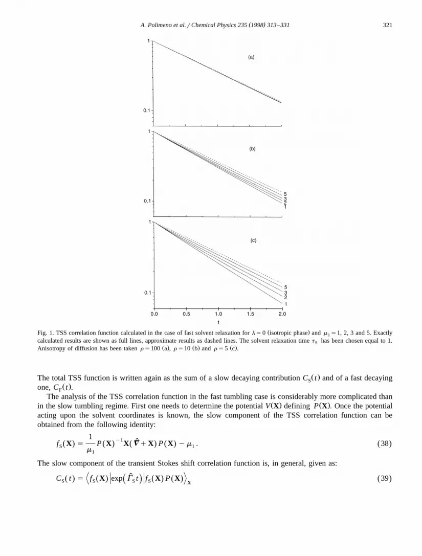
In the case of fast relaxing solvent coordinates, the TSS depends essentially on the fast decay of the polarisation,disregarding the probe orientation. Naturally, this limiting regime is reached only when the anisotropy of

Ž .diffusion is relatively large. In Fig. 1 we compare the analytical prediction of Eq. 32 with the exact result forŽ .C t , for an isotropic medium, ls0, choosing m equal to 1, 2, 3 and 5. In Fig. 2 analogous results are1

Ž .presented for an oriented phase, ls2. In both cases the TSS is calculated for t s1 and rs100 a , rs10SŽ . Ž .b and rs5 c . The comparison with the exact calculations shows that the analytical prediction based on thehypothesis of fast solvent is considerably better when rather high dipole moments are employed.

3.2. Fast tumbling

We shall consider next the dynamical regime characterised by fast tumbling motion and relatively slowsolvent relaxation, i.e. t 0t , or r(1. Notice that although the standard interpretation of dynamical StokesR S

shift effects is usually based on the previously discussed regime, slow tumbling versus fast solvent relaxation, incomplex solvents the dielectric relaxation times can be of the order of hundreds of picoseconds, i.e. comparablewith the rotational correlation time of the solute molecule. It is then justified to treat the fast tumbling case as amore representative asymptotic description of actual solvation dynamics processes in nematics or in isotropicphase close to the isotropic-nematic transition.

Again we define an averaged time evolution operator for the slow coordinates, which are now given by X

1 y1trˆ ˆ ˆG sy = P X = P X 35Ž . Ž . Ž .St S

Ž .where P X is obtained averaging P with respect to V:eq

P q sP X . 36² :Ž . Ž . Ž .eq V

The fast coordinates time evolution operator is now given by:

1tr y1G sy m P m P . 37Ž .ˆ ˆF eq eq

t R


Ž .Fig. 1. TSS correlation function calculated in the case of fast solvent relaxation for ls0 isotropic phase and m s1, 2, 3 and 5. Exactly1

calculated results are shown as full lines, approximate results as dashed lines. The solvent relaxation time t has been chosen equal to 1.SŽ . Ž . Ž .Anisotropy of diffusion has been taken r s100 a , r s10 b and r s5 c .

Ž .The total TSS function is written again as the sum of a slow decaying contribution C t and of a fast decayingSŽ .one, C t .F

The analysis of the TSS correlation function in the fast tumbling case is considerably more complicated thanŽ . Ž .in the slow tumbling regime. First one needs to determine the potential V X defining P X . Once the potential

acting upon the solvent coordinates is known, the slow component of the TSS correlation function can beobtained from the following identity:

1 y1 ˆf X s P X X =qX P X ym . 38Ž . Ž . Ž . Ž .Ž .S 1m1

The slow component of the transient Stokes shift correlation function is, in general, given as:

ˆC t s f X exp G t f X P X 39Ž . Ž . Ž . Ž . Ž .¦ ;Ž .S S S S X


Ž .Fig. 2. TSS correlation function calculated in the case of fast solvent relaxation for ls2 nematic phase and m s1, 2, 3 and 5. Exactly1

calculated results are shown as full lines, approximate results as dashed lines. The solvent relaxation time t has been chosen equal to 1.SŽ . Ž . Ž .Anisotropy of diffusion has been taken r s100 a , r s10 b and r s5 c .

Ž .and its zero value C 0 gives the overall weight of the slow decaying term, which is a function ranging from 0,S

corresponding to vanishing dipole m ™0, to 1, corresponding to the case of large dipole m ™`: i.e. the1 1

weight of the solvent slow component is negligible for weak coupling, and it is dominant for strong coupling.Ž .This conclusion can be obtained both for the isotropic and the ordered phases see below . To proceed, we need

Ž .to calculate explicitly the potential V X ; for general values of l an analytical expression is not available.However we can expand the potential in powers of the parameter l and calculate the expansion coefficients:

V X sV X qlV X ql2V X q . . . . 40Ž . Ž . Ž . Ž . Ž .0 1 2

Ž .The explicit form for the coefficients of Eq. 40 can be found in Appendix C. If we truncate the expansion ofthe potential to the first-order term we obtain:

V X sV X qlV X P cosu 41Ž . Ž . Ž . Ž . Ž .0 1 2


Ž . Ž . Ž . Ž .Fig. 3. Functions V X a and V X b calculated for m s1, 2, 3, 5 and 10.0 1 1

Ž . Ž .where V X and V X are given by0 1

sinhm X11 2V X s X y ln 42Ž . Ž .0 2m X1

3 coth m X 31V X sy 1y q 43Ž . Ž .1 2 2ž /m X m X1 1

Ž .where X,u ,f are the polar coordinates of vector X in the LF. This expansion becomes obviously exact forls0, isotropic case, where only a dependence upon the modulus X is retained. In the nematic phase, theaveraged potential acting on the solvent contains an explicit dependence upon the polar angle u . Minima are

Ž .located at us0,p , corresponding to X parallel to the director. Finally, f X is obtained in a similar manner inS

the form:

f X s f X ql f X P cosu 44Ž . Ž . Ž . Ž . Ž .S 0 1 2

Ž . Ž .where f X and f X are given by0 1

X 1f X s y ym 45Ž . Ž .0 1tanh m X m1 1

3 coth m X 212f X sy 1ycoth m Xy q 46Ž . Ž .1 1 2 2ž /m m X m X1 1 1

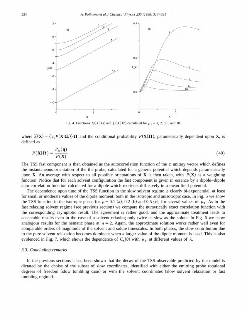
Ž . Ž . Ž . Ž .In Figs. 3 and 4 we show functions V X , V X , f X and f X for several values of m . The isotropic part0 1 0 1 1Ž . Ž .2of the effective potential, V X , goes to the limit Xym r2 for m ™`, i.e. for a high dipole moment the0 1 1

Ž .solvent polarisation fluctuates around the dipole value. The correction term in the anisotropic phase, V X goes1

to the limit of unity for large dipoles.The fast probe component has a non-zero weight, which can be relevant for small dipole moments. Following

Appendix B one gets2ˆ <C t s HdX P X z exp yG t z P X V yz X 47Ž . Ž . Ž . Ž . Ž .¦ ;Ž .ÝF i F i V i

i


Ž . Ž . Ž . Ž .Fig. 4. Functions f X a and f X b calculated for m s1, 2, 3, 5 and 10.0 1 1

Ž . ² Ž < .: Ž < .where z X s z P X V V and the conditional probability P X V , parametrically dependent upon X, isi i

defined as

P qŽ .eq<P X V s 48Ž . Ž .

P XŽ .The TSS fast component is then obtained as the autocorrelation function of the z unitary vector which definesthe instantaneous orientation of the the probe, calculated for a generic potential which depends parametrically

Ž .upon X. An average with respect to all possible orientations of X is then taken, with P X as a weightingfunction. Notice that for each solvent configuration the fast component is given in essence by a dipole–dipoleauto-correlation function calculated for a dipole which reorients diffusively in a mean field potential.

The dependence upon time of the TSS function in the slow solvent regime is clearly bi-exponential, at leastfor small or moderate values of the dipole moment, both in the isotropic and anisotropic case. In Fig. 5 we show

Ž . Ž . Ž .the TSS function in the isotropic phase for rs0.1 a , 0.2 b and 0.5 c , for several values of m . As in the1Ž .fast relaxing solvent regime see previous section we compare the numerically exact correlation function with

the corresponding asymptotic result. The agreement is rather good, and the approximate treatment leads toacceptable results even in the case of a solvent relaxing only twice as slow as the solute. In Fig. 6 we showanalogous results for the nematic phase at ls2. Again, the approximate solution works rather well even forcomparable orders of magnitude of the solvent and solute timescales. In both phases, the slow contribution dueto the pure solvent relaxation becomes dominant when a larger value of the dipole moment is used. This is also

Ž .evidenced in Fig. 7, which shows the dependence of C 0 with m , at different values of l.S 1

3.3. Concluding remarks

In the previous sections it has been shown that the decay of the TSS observable predicted by the model isdictated by the choise of the subset of slow coordinates, identified with either the emitting probe rotational

Ž . Ždegrees of freedom slow tumbling case or with the solvent coordinates slow solvent relaxation or fast.tumbling regime .


Ž .Fig. 5. TSS correlation function calculated in the case of slow solvent relaxation for ls0 isotropic phase and m s1, 2, 3 and 5. Exactly1

calculated results are shown as full lines, approximate results as dashed lines. The solvent relaxation time t has been chosen equal to 1.SŽ . Ž . Ž .Anisotropy of diffusion has been taken r s0.1 a , r s0.2 b and r s0.5 c .

In the case of slow tumbling, the TSS correlation function depends only upon the solvent dynamicsrepresented by the polarisation vector X. On the timescale of the fast solvent relaxation the orientation of theprobe dipole z is essentially fixed, so that the polarisation vector X is able to explore all the possibleconfiguration in the phase space, till the equilibrium configuration Xsm z is reached, with a relaxation time1

t s1rD .S S

In the fast tumbling regime two components, one related to the solvent relaxation and the other describing thesolute rotation, are always predicted. Let us first consider the fast relaxing contribution to the TSS observable inan isotropic phase. For a fixed configuration of the solvent coordinate X, the potential acting on the solutemolecule is given by a first-order Legendre polynomial in cosb

X, where bX is the angle between z and X, and it

is proportional to m : a minimum at bX s0 is predicted, i.e. the solute molecule has a preferential orientation1

parallel to the solvent polarisation. When the value of m is increased both the curvature and the depth of the1

well are increased. As a consequence the solute relaxes faster and within a narrower distribution of orientationsaround b

X s0. When m becomes very large the weight of the fast component due to the tumbling motion is1


Ž .Fig. 6. TSS correlation function calculated in the case of slow solvent relaxation for ls2 nematic phase and m s1, 2, 3 and 5. Exactly1

calculated results are shown as full lines, approximate results as dashed lines. The solvent relaxation time t has been chosen equal to 1.SŽ . Ž . Ž .Anisotropy of diffusion has been taken r s0.1 a , r s0.2 b and r s0.5 c .

Ž . Ž . Ž . Ž .Fig. 7. Plot in logarithmic scale of C 0 versus m for ls0 squares , 2 circles and 3 triangles .S 1


Ž .negligible. Let us now consider the slow relaxing contribution C t , still in the isotropic phase. This isSŽ . Ž .dependent upon the averaged potential function V X given by Eq. 42 and upon the averaged observable0

Ž .given by Eq. 45 . The potential has a single minimum which for large dipole values is located at Xsm . The1

solvent relaxation is then essentially described as the equilibration of the modulus of the polarisation to m .1

In the nematic phase a simple dependence upon the polar angle u , which gives the solvent polarisationorientation with respect to the director, is introduced in the averaged potential as well as in the averaged

Ž Ž . Ž .. Ž .observable cf. Eqs. 43 and 46 . This is only a correction term to the isotropic term cf. Figs. 3b and 4b andthe same analysis used in the isotropic phase can be adopted, at least for small values of the mean fieldparameter l. The dependence upon the u angle becomes more important for large values of l, which is in anycase always confined to a few k T units, at least for common nematogens.B

To summarize, our results suggest that an augmented stochastic model, describing the rotational motion of afluorescent probe coupled to a solvent coordinate, can be used to interpret time-dependent Stokes shiftexperiments in isotropic liquids and liquid crystals, despite the significant number of independent variables

Ž .included in the model the set of Euler angles plus the three components of the solvent coordinate . Fullnumerical solutions are indeed available, but it is of relevance to notice that working approximate treatments areconceivable, which can cover several dynamical regimes. This is encouraging when extensions of the model areconsidered, like inclusion of inertial effects, coupling to relaxing local solvent structures and interaction betweentranslational and rotational degrees of freedom: effective approximate solutions based on projection formalisms,which take into account differences in timescales, are then the only practical tool to extract useful informationfrom the model.

Acknowledgements

Support has been provided by the Italian Ministry for Universities and Scientific and Technological Researchand the HCM contract N. ERBCHRXCT930282, and in part by the Italian National Research Council throughits Centro Studi sugli Stati Molecolari and the Committee for Information Science and Technology.

Appendix A. Derivation of the F tensor

Ž . Ž .For a generic ellipsoidal body and cavity of volume V, the F tensor is written in SI units :

1 y1X X Y X Y1r2 y1r2Fs ´ ýn ý1 1yn ´ n yn 1yn ´ 49Ž . Ž . Ž . Ž .´ V0

where n is the electrostatic depolarisation tensor for an ellipsoidal empty cavity surrounded by the dielectric; nX

is the electrostatic depolarisation tensor for an ellipsoidal cavity filled by the dielectric, in vacuo; nY is simplyý1r2 n ´ 1r2.

Ž .Operatively, ´ is diagonal by definition in the LF, with principal values ´ is1,2,3 . The depolarisationi

tensor for the cavity, is defined with respect to the auxiliary tensor M for the ellipsoid; in the LFMŽL.sEay2 Etr, and a is the diagonal tensor whose principal values are the semi-axes of the cavity, while E isthe Euler matrix which transforms a vector from the MF to the LF.

The representations of n in the LF and MF are analogously related, nŽL.sEnŽM.Etr, where the principalvalues nŽM. are given in terms of a. Similarly, nX is defined in terms of an auxiliary tensor MX, which in the LFis MXŽL.s´ 1r2 MŽL. 1r2. For the case of a spherical cavity, asa1, nŽL.snŽM.s1r3, MXŽL.s´ra2. Thus nX isdiagonal in the LF, too, with components:

`´ 1iXn s d z 50Ž .Hi 1r22 0 1q´ z 1q´ z 1q´ z 1q´ zŽ . Ž . Ž . Ž .i 1 2 3


and F is also diagonal in the LF, with components:

1 1ynX´ y2nXŽ .i i i

F s . 51Ž .Xi 3 ´ yn ´ y14p a ´ Ž .i i i0

By choosing ´ s´ s´ and ´ s´ the formulas reported in the main text are obtained.1 2 H 3 5

Appendix B. Timescales separation

Let us consider a generic set of coordinates, q, which can be partitioned in two subsets q and q ,F S

respectively fast and slow relaxing. We want to evaluate the following generic correlation function:

1r2 1r2˜G t s f q P q exp yG g q P q 52:Ž . Ž . Ž . Ž . Ž . Ž .Ž .¦ ;ˆŽ . Ž .where P q is the equilibrium distribution of the system; the unsymmetrized time evolution operator is G ,

˜ ˜ y1r2 ˆ 1r2 ˜Ž . Ž . w x Ž .while G is the symmetrized operator, GsP q G P q 12,13 . The symmetrized forms of G t , G are˜ ˜simply introduced for convenience. We suppose to be able to separate from G an operator G , acting on qF F

only, depending parametrically upon q , which is responsible for the relaxation of the fast variables when qS S˜are frozen; the residual operator is indicated by d G :

˜ ˜ ˜GsG qdG . 53Ž .F

˜We may write G in its spectral decomposed form:F

˜ < : ² <Gs n E q n 54Ž . Ž .Ý F n Sn

˜< :where n are the orthonormal eigenfunctions of G , parametrically depending upon q . Notice that the firstF F SŽeigenvalue E s0 vanishes and corresponds to the stationary solution equilibrium distribution of the fast0

.coordinates when the slow coordinates are frozen :

P q P qŽ . Ž .<P q q s s 55Ž .Ž .S F ² :P q P qŽ . Ž .F S S

Ž .Under the equivalent of the Born–Oppenheimer BO approximation usually applied to the quantum mechanicaltreatment of the coupled motion of electrons and nuclei in molecules, we may expand the total time evolution

< : Žoperator in the n basis set, and introduce the following simplified matrix representation in the q spaceF F˜. w xonly of d G 12,13 :

BOX˜ ˜ ˜< < < <X X² : ² :n dG n s d n dG n sd G . 56Ž .n ,n n ,n nF F

Ž . < :Notice that Eq. 56 , in most cases, is equivalent to assume that the gradient of n with respect to the fastF

variables is negligible, at least when the dependence upon the equilibrium distribution has been considered. Forinstance, when studying a completely diffusional problem, we get:

E Ey1r2 y1r2G syP q D P q P q 57Ž . Ž . Ž . Ž .F Fž / ž /Eq EqF F

E Ey1r2 y1r2˜dGsyP q D P q P q . 58Ž . Ž . Ž . Ž .Sž / ž /Eq EqS S


˜The nth eigenfunction of G can be written:F

1r2P qŽ .

< :n sH q 59Ž . Ž .F n P qŽ .S S

Ž .If functions H q are weakly dependent upon q :n S

E< :n f0 60Ž .Fž /EqS

then it is shown that:

E EX y1r2 y1r2˜< < X² :n dG n syP q D P q P q d 61Ž . Ž . Ž . Ž .S S S S S S nnF ž / ž /Eq EqS S

X ˜for all couples n,n , i.e. in this particular case even the dependence of G upon n can be neglected. Followingnw xthe complete derivation of Ref. 27 , one can show that the BO approximation of the correlation function is:

`˜1r2 yŽE qG . t 1r2n n< <² : ² :G t s fP n e n gP . 62² :Ž . Ž .ÝBO F F S

ns0

Several degrees of approximations are now available. First of all we may consider that the separation oftimescales between the two subsets of variables is complete, i.e. for all eigenvalues, except the first, ns0, thefollowing inequality holds:

˜< <E q 4 G . 63Ž . Ž .n S n

w xIn this case the correlation function can be written as a sum of two terms 27

G t sG t qG t 64Ž . Ž . Ž . Ž .BO S F

˜1r2 yG t 1r20< <G t s f P e g P 65² :Ž . Ž .S S S S S S

˜1r2 yG t 1r2F< <G t s fy f P e gyg P 66² :Ž . Ž . Ž . Ž .F S S

Ž . Ž . ² Ž . Ž .:where f q P q s f q P q . The total correlation function is given as the sum of a slow relaxingFS S S S

contribution, and of the inhomogeneous average of a fast relaxing contribution.A weaker approximation may be necessary, if the timescale separation is not complete; this happens, for

˜instance, if some eigenmodes of G are associated with kinetic processes, i.e. relaxation of metastable statesFŽ . Ž . Ž .separated by finite energetic barriers. Let us suppose that E -E q - . . . -E q <E q - . . . , i.e.0 1 S N S N q1 SS S

let us separate the first set of N ‘small’ eigenvalues from the remaining set of ‘large’ eigenvalues. Then weSŽ .apply Eq. 63 only to the set of large eigenvalues. The correlation function will be still obtained as the sum of a

slow relaxing and a fast relaxing term, but now they are written as:

NS˜1r2 yŽE qG . t 1r2n n< <² : ² :G t s fP n e n gP 67² :Ž . Ž .ÝS F F S

ns0

N NS S˜1r2 1r2 yG t 1r2 1r2F< ² < < : <² : ² :G t s fP y fP n n e gP y n n gP . 68Ž . Ž .Ý Ý FF F F¦ ;

ns0 ns0 S

Additional approximation can be made, for instance neglecting the explicit dependence upon q of E .S n


( )Appendix C. Expansion coefficients for the potential V X

Ž .The l-expansion of the effective potential V X is obtained as follows. The potential is written formally as:tr 2V X sylnHdV exp lP cosb qm z X sV X qlV X ql V X q . . . 69Ž . Ž . Ž . Ž . Ž . Ž .2 1 0 1 2

Ž . Ž .where Vs a ,b are the angles defining the orientation of the unitary vector z the long molecular axis in theLF. The n-term is defined as

1 dn

<V X s V X . 70Ž . Ž . Ž .ls0n nn! dl

The first two terms are

V X sylnHdV exp m z tr X 71Ž . Ž .Ž .0 1

HdVP cosb exp m z tr XŽ . Ž .2 1V X sy 72Ž . Ž .1 trHdV exp m z XŽ .1

X Ž X X.We can change the variables of integration from V to V s a ,b formally defined as the angles specifyingthe orientation of z with respect to X. The zero-order term is then:

p sinhm X1X X X1 12 2V X s X y ln db sinb exp m X cosb s X y ln 73Ž . Ž . Ž .H0 12 2m X0 1

and the first-order term is obtained as

HdbX sinb

X P cosbX exp m X cosb

X 3coth m X 3Ž . Ž .2 1 1V X s P cosu sy 1y q P cosu .Ž . Ž . Ž .X X X1 2 22 2ž /Hdb sinb exp m X cosb m X m XŽ .1 1 1

74Ž .

References

w x Ž .1 M. Maroncelli, J. Chem. Phys. 94 1991 2084.w x Ž .2 P.V. Kumar, M. Maroncelli, J. Chem. Phys. 103 1995 3038.w x Ž .3 R. Biswas, N. Nandi, B. Bagchi, J. Phys. Chem. B 101 1997 2968.w x Ž .4 K. Ando, J. Chem. Phys. 107 1997 4585.w x Ž .5 H.A. Kramers, Physica 7 1946 284.w x Ž .6 R.E.D. McClung, J. Chem. Phys. 75 1981 5503.w x Ž .7 J.S. Hwang, R.P. Mason, L.P. Hwang, J.H. Freed, J. Chem. Phys. 79 1975 489.w x Ž .8 H.W. Spiess, Rotational Dynamics of Small and Macromolecules, in: T. Dorfmuller, R. Pecora Eds. , Lecture Notes in Physics

Ž .Springer, Berlin, 1987 p. 89.w x Ž .9 V.I. Melnikov, S.V. Meshkov, J. Chem. Phys. 85 1986 1018.

w x Ž .10 V.I. Melnikov, Phys. Rep. 209 1991 1.w x Ž .11 D. Braun, P.L. Nordio, A. Polimeno, G. Saielli, Chem. Phys. 208 1996 127.w x Ž .12 A. Polimeno, G.J. Moro, J.H. Freed, J. Chem. Phys. 104 1996 104.w x Ž .13 A. Polimeno, G.J. Moro, J.H. Freed, J. Chem. Phys. 102 1995 9094.w x Ž .14 P.L. Nordio, A. Polimeno, Mol. Phys. 75 1992 1203.w x Ž .15 A. Polimeno, P.L. Nordio, Chem. Phys. Lett. 192 1992 509.w x16 G.J. Moro, A. Polimeno, manuscript submitted.w x Ž .17 L. Feltre, A. Polimeno, G. Saielli, P.L. Nordio, Mol. Cryst. Liq. Cryst. 290 1996 163.w x Ž .18 G. Saielli, A. Polimeno, P.L. Nordio, P. Bartolini, M. Ricci, R. Righini, J. Chem. Soc. Faraday Trans. 94 1998 121.w x Ž .19 T.J. Kang, W. Jarzeba, P.F. Barbara, T. Fonseca, Chem. Phys. 149 1990 81.w x Ž .20 C. Zannoni, Mol. Phys. 38 1979 1813.


w x Ž .21 A. Polimeno, A. Barbon, P.L. Nordio, W. Rettig, J. Phys. Chem. 98 1994 12158.w x Ž .22 M. Maroncelli, R.S. Fee, C.F. Chapman, G.R. Fleming, J. Phys. Chem. 95 1991 1012.w x23 C. Ferrante, J. Rau, F.W. Deeg, C. Brauchle, J. Luminesc. Proc. DPC 1997, in press.¨w x Ž .24 U. Segre, Mol. Cryst. Liq. Cryst. 90 1982 239.w x Ž .25 A. Chelkowski, Dielectric Physics Elsevier, Amsterdam, 1980 .w x Ž .26 A. Arcioni, F. Bertinelli, R. Tarroni, C. Zannoni, Mol. Phys. 61 1987 1161.w x Ž .27 A. Polimeno, G.J. Moro, J.H. Freed, J. Chem. Phys. 104 1995 1090.w x Ž .28 B. Bagchi, D.W. Oxtoby, G.R. Fleming, Chem. Phys. 86 1984 257.

a diffusive model for interpreting solvation dynamics in isotropic and ordered liquid phases

Documents