S

A

A

Pa

b

c

ARAA

JGCCC

KVVR

1

iSoNttotu

tmt(aarb

(

2h

ARTICLE IN PRESSG ModelRFE-22; No. of Pages 18

The Spanish Review of Financial Economics xxx (2013) xxx–xxx

The Spanish Review of Financial Economics

www.elsev ier .es /s r fe

rticle

comprehensive review of Value at Risk methodologies�

ilar Abada, Sonia Benitob,∗, Carmen Lópezc

Universidad Rey Juan Carlos and IREA-RFA, Paseo Artilleros s/n, 28032 Madrid, SpainUniversidad Nacional de Educación a Distancia (UNED), Senda del Rey 11, 28223 Madrid, SpainUniversidad Nacional de Educación a Distancia (UNED), Spain

a r t i c l e i n f o

rticle history:eceived 5 October 2012ccepted 28 June 2013vailable online xxx

EL classification:3214

a b s t r a c t

In this article we present a theoretical review of the existing literature on Value at Risk (VaR) specificallyfocussing on the development of new approaches for its estimation. We effect a deep analysis of the Stateof the Art, from standard approaches for measuring VaR to the more evolved, while highlighting theirrelative strengths and weaknesses. We will also review the backtesting procedures used to evaluate VaRapproach performance. From a practical perspective, empirical literature shows that approaches basedon the Extreme Value Theory and the Filtered Historical Simulation are the best methods for forecastingVaR. The Parametric method under skewed and fat-tail distributions also provides promising results

1522

eywords:alue at Riskolatility

especially when the assumption that standardised returns are independent and identically distributed isset aside and when time variations are considered in conditional high-order moments. Lastly, it appearsthat some asymmetric extensions of the CaViaR method provide results that are also promising.

© 2012 Asociación Espanola de Finanzas. Published by Elsevier España, S.L. All rights reserved.

2001).Among Parametric approaches, the first model for VaR estima-

tion is Riskmetrics, from Morgan (1996). The major drawback of this

isk management

. Introduction

Basel I, also called the Basel Accord, is the agreement reachedn 1988 in Basel (Switzerland) by the Basel Committee on Bankupervision (BCBS), involving the chairmen of the central banksf Germany, Belgium, Canada, France, Italy, Japan, Luxembourg,etherlands, Spain, Sweden, Switzerland, the United Kingdom and

he United States of America. This accord provides recommenda-ions on banking regulations with regard to credit, market andperational risks. Its purpose is to ensure that financial institu-ions hold enough capital on account to meet obligations and absorbnexpected losses.

For a financial institution measuring the risk it faces is an essen-ial task. In the specific case of market risk, a possible method of

easurement is the evaluation of losses likely to be incurred whenhe price of the portfolio assets falls. This is what Value at RiskVaR) does. The portfolio VaR represents the maximum amountn investor may lose over a given time period with a given prob-

Please cite this article in press as: Abad, P., et al. A comprehensive revihttp://dx.doi.org/10.1016/j.srfe.2013.06.001

bility. Since the BCBS at the Bank for International Settlementsequires a financial institution to meet capital requirements on theasis of VaR estimates, allowing them to use internal models for

� This work has been funded by the Spanish Ministerio de Ciencia y TecnologíaECO2009-10398/ECON and ECO2011-23959).∗ Corresponding author.

E-mail addresses: pilar.abad@urjc.es (P. Abad), soniabm@cee.uned.es (S. Benito).

173-1268/$ – see front matter © 2012 Asociación Espanola de Finanzas. Published by Elttp://dx.doi.org/10.1016/j.srfe.2013.06.001

VaR calculations, this measurement has become a basic marketrisk management tool for financial institutions.2 Consequently, itis not surprising that the last decade has witnessed the growth ofacademic literature comparing alternative modelling approachesand proposing new models for VaR estimations in an attempt toimprove upon those already in existence.

Although the VaR concept is very simple, its calculation is noteasy. The methodologies initially developed to calculate a portfo-lio VaR are (i) the variance–covariance approach, also called theParametric method, (ii) the Historical Simulation (Non-parametricmethod) and (iii) the Monte Carlo simulation, which is a Semi-parametric method. As is well known, all these methodologies,usually called standard models, have numerous shortcomings,which have led to the development of new proposals (see Jorion,

ew of Value at Risk methodologies. Span Rev Financ Econ. (2013).

2 When the Basel I Accord was concluded in 1988, no capital requirement wasdefined for the market risk. However, regulators soon recognised the risk to a bank-ing system if insufficient capital was held to absorb the large sudden losses fromhuge exposures in capital markets. During the mid-90s, proposals were tabled foran amendment to the 1988 accord, requiring additional capital over and above theminimum required for credit risk. Finally, a market risk capital adequacy frame-work was adopted in 1995 for implementation in 1998. The 1995 Basel I Accordamendment provided a menu of approaches for determining the market risk capitalrequirements.

sevier España, S.L. All rights reserved.

ING ModelS

2 f Finan

mEnma(s

hmoinrt

pwIhbEdatWmTwb

rIrasrod

2

eatcoIn

tarrt

mtmd

ARTICLERFE-22; No. of Pages 18

P. Abad et al. / The Spanish Review o

odel is the normal distribution assumption for financial returns.mpirical evidence shows that financial returns do not follow aormal distribution. The second relates to the model used to esti-ate financial return conditional volatility. The third involves the

ssumption that return is independent and identically distributediid). There is substantial empirical evidence to demonstrate thattandardised financial returns distribution is not iid.

Given these drawbacks research on the Parametric methodas moved in several directions. The first involves finding aore sophisticated volatility model capturing the characteristics

bserved in financial returns volatility. The second line of researchnvolves searching for other density functions that capture skew-ess and kurtosis of financial returns. Finally, the third line ofesearch considers that higher-order conditional moments areime-varying.

In the context of the Non-parametric method, several Non-arametric density estimation methods have been implemented,ith improvement on the results obtained by Historical Simulation.

n the framework of the Semi-parametric method, new approachesave been proposed: (i) the Filtered Historical Simulation, proposedy Barone-Adesi et al. (1999); (ii) the CaViaR method, proposed byngle and Manganelli (2004) and (iii) the conditional and uncon-itional approaches based on the Extreme Value Theory. In thisrticle, we will review the full range of methodologies developedo estimate VaR, from standard models to those recently proposed.

e will expose the relative strengths and weaknesses of theseethodologies, from both theoretical and practical perspectives.

he article’s objective is to provide the financial risk researcherith all the models and proposed developments for VaR estimation,

ringing him to the limits of knowledge in this field.The paper is structured as follows. In the next section, we

eview a full range of methodologies developed to estimate VaR.n Section 2.1, a non-parametric approach is presented. Paramet-ic approaches are offered in Section 2.2, and semi-parametricpproaches in Section 2.3. In Section 3, the procedures for mea-uring VaR adequacy are described and in Section 4, the empiricalesults obtained by papers dedicated to comparing VaR method-logies are shown. In Section 5, some important topics of VaR areiscussed. The last section presents the main conclusions.

. Value at Risk methods

According to Jorion (2001), “VaR measure is defined as the worstxpected loss over a given horizon under normal market conditionst a given level of confidence. For instance, a bank might say thathe daily VaR of its trading portfolio is $1 million at the 99 percentonfidence level. In other words, under normal market conditions,nly one percent of the time, the daily loss will exceed $1 million.”n fact the VaR just indicates the most we can expect to lose if noegative event occurs.

The VaR is thus a conditional quantile of the asset return loss dis-ribution. Among the main advantages of VaR are simplicity, widepplicability and universality (see Jorion, 1990, 1997).3 Let r1, r2,3,. . ., rn be identically distributed independent random variablesepresenting the financial returns. Use F(r) to denote the cumula-

Please cite this article in press as: Abad, P., et al. A comprehensive revihttp://dx.doi.org/10.1016/j.srfe.2013.06.001

ive distribution function, F(r) = Pr(r < r|˝t − 1) conditionally on the

3 There is another market risk measurement, called Expected Shortfall (ES). ESeasures the expected value of our losses if we get a loss in excess of VaR. So that,

his measure tells us what to expect in a bad estate, while the VaR tells us nothingore than to expect a loss higher than the VaR itself. In Section 5, we will formally

efine this measure besides presenting some criticisms of VaR measurement.

PRESScial Economics xxx (2013) xxx–xxx

information set ˝t − 1 that is available at time t − 1. Assume that{rt} follows the stochastic process:

rt = � + εt

εt = zt�t zt∼iid(0, 1)(1)

where �2t = E(z2

t |˝t−1) and zt has the conditional distribution func-tion G(z), G(z) = Pr(zt < z|˝t−1). The VaR with a given probability

∈ (0, 1), denoted by VaR(˛), is defined as the quantile of theprobability distribution of financial returns: F(VaR(˛)) = Pr(rt <VaR(˛)) = or VaR(˛) = inf{v|P(rt ≤ v) = ˛}.

This quantile can be estimated in two different ways: (1) invert-ing the distribution function of financial returns, F(r), and (2)inverting the distribution function of innovations, with regard toG(z) the latter, it is also necessary to estimate �2

t .

VaR(˛) = F−1(˛) = � + �tG−1(˛) (2)

Hence, a VaR model involves the specifications of F(r) or G(z).The estimation of these functions can be carried out using thefollowing methods: (1) non-parametric methods; (2) parametricmethods and (3) semi-parametric methods. Below we will describethe methodologies, which have been developed in each of thesethree cases to estimate VaR.4

2.1. Non-parametric methods

The Non-parametric approaches seek to measure a portfolio VaRwithout making strong assumptions about returns distribution. Theessence of these approaches is to let data speak for themselves asmuch as possible and to use recent returns empirical distribution– not some assumed theoretical distribution – to estimate VaR.

All Non-parametric approaches are based on the underlyingassumption that the near future will be sufficiently similar to therecent past for us to be able to use the data from the recent past toforecast the risk in the near future.

The Non-parametric approaches include (a) Historical Simula-tion and (b) Non-parametric density estimation methods.

2.1.1. Historical simulationHistorical Simulation is the most widely implemented Non-

parametric approach. This method uses the empirical distributionof financial returns as an approximation for F(r), thus VaR(˛) isthe quantile of empirical distribution. To calculate the empiri-cal distribution of financial returns, different sizes of samples canbe considered.

The advantages and disadvantages of the Historical Simulationhave been well documented by Down (2002). The two main advan-tages are as follows: (1) the method is very easy to implement,and (2) as this approach does not depend on parametric assump-tions on the distribution of the return portfolio, it can accommodatewide tails, skewness and any other non-normal features in finan-cial observations. The biggest potential weakness of this approach isthat its results are completely dependent on the data set. If our dataperiod is unusually quiet, Historical Simulation will often underes-timate risk and if our data period is unusually volatile, HistoricalSimulation will often overestimate it. In addition, Historical Simu-lation approaches are sometimes slow to reflect major events, suchas the increases in risk associated with sudden market turbulence.

The first papers involving the comparison of VaR methodolo-

ew of Value at Risk methodologies. Span Rev Financ Econ. (2013).

gies, such as those by Beder (1995, 1996), Hendricks (1996), andPritsker (1997), reported that the Historical Simulation performedat least as well as the methodologies developed in the early years,

4 For a more pedagogic review of some of these methodologies (see FeriaDomínguez, 2005).

ING ModelS

f Finan

tcoo

((VprtacH

2

utdliibdhialodwcB

MwwSsst

weptdaFV

2

cAwtm

ccl

ARTICLERFE-22; No. of Pages 18

P. Abad et al. / The Spanish Review o

he Parametric approach and the Monte Carlo simulation. The mainonclusion of these papers is that among the methodologies devel-ped initially, no approach appeared to perform better than thethers.

However, more recent papers such as those by Abad and Benito2013), Ashley and Randal, 2009, Trenca (2009), Angelidis et al.2007), Alonso and Arcos (2005), Gento (2001), Danielsson and deries (2000) have reported that the Historical Simulation approachroduces inaccurate VaR estimates. In comparison with otherecently developed methodologies such as the Historical Simula-ion Filtered, Conditional Extreme Value Theory and Parametricpproaches (as we become further separated from normality andonsider volatility models more sophisticated than Riskmetrics),istorical Simulation provides a very poor VaR estimate.

.1.2. Non-parametric density estimation methodsUnfortunately, the Historical Simulation approach does not best

tilise the information available. It also has the practical drawbackhat it only gives VaR estimates at discrete confidence intervalsetermined by the size of our data set.5 The solution to this prob-

em is to use the theory of Non-parametric density estimation. Thedea behind Non-parametric density is to treat our data set as ift were drawn from some unspecific or unknown empirical distri-ution function. One simple way to approach this problem is toraw straight lines connecting the mid-points at the top of eachistogram bar. With these lines drawn the histogram bars can be

gnored and the area under the lines treated as though it was a prob-bility density function (pdf) for VaR estimation at any confidenceevel. However, we could draw overlapping smooth curves and son. This approach conforms exactly to the theory of non-parametricensity estimation, which leads to important decisions about theidth of bins and where bins should be centred. These decisions

an therefore make a difference to our results (for a discussion, seeutler and Schachter (1998) or Rudemo (1982)).

A kernel density estimator (Silverman, 1986; Sheather andarron, 1990) is a method for generalising a histogram constructedith the sample data. A histogram results in a density that is piece-ise constant where a kernel estimator results in smooth density.

moothing the data can be performed with any continuous shapepread around each data point. As the sample size grows, the netum of all the smoothed points approaches the true pdf whateverhat may be irrespective of the method used to smooth the data.

The smoothing is accomplished by spreading each data pointith a kernel, usually a pdf centred on the data point, and a param-

ter called the bandwidth. A common choice of bandwidth is thatroposed by Silverman (1986). There are many kernels or curveso spread the influence of each point, such as the Gaussian kernelensity estimator, the Epanechnikov kernel, the biweight kernel,n isosceles triangular kernel and an asymmetric triangular kernel.rom the kernel, we can calculate the percentile or estimate of theaR.

.2. Parametric method

Parametric approaches measure risk by fitting probabilityurves to the data and then inferring the VaR from the fitted curve.

Please cite this article in press as: Abad, P., et al. A comprehensive revihttp://dx.doi.org/10.1016/j.srfe.2013.06.001

mong Parametric approaches, the first model to estimate VaRas Riskmetrics from Morgan (1996). This model assumes that

he return portfolio and/or the innovations of return follow a nor-al distribution. Under this assumption, the VaR of a portfolio at

5 Thus, if we have, e.g., 100 observations, it allows us to estimate VaR at the 95%onfidence level but not the VaR at the 95.1% confidence level. The VaR at the 95%onfidence level is given by the sixth largest loss, but the VaR at the 95.1% confidenceevel is a problem because there is no loss observation to accompany it.

PRESScial Economics xxx (2013) xxx–xxx 3

an 1 − ˛% confidence level is calculated as VaR(˛) = � + �tG−1(˛),where G−1(˛) is the quantile of the standard normal distributionand �t is the conditional standard deviation of the return portfo-lio. To estimate �t, Morgan uses an Exponential Weight MovingAverage Model (EWMA). The expression of this model is as follows:

�2t (1 − �)

N−1∑j=0

�j(εt−j)2 (3)

where � = 0.94 and the window size (N) is 74 days for daily data.The major drawbacks of Riskmetrics are related to the normal

distribution assumption for financial returns and/or innovations.Empirical evidence shows that financial returns do not follow nor-mal distribution. The skewness coefficient is in most cases negativeand statistically significant, implying that the financial return dis-tribution is skewed to the left. This result is not in accord withthe properties of a normal distribution, which is symmetric. Also,empirical distribution of financial return has been documented toexhibit significantly excessive kurtosis (fat tails and peakness) (seeBollerslev, 1987). Consequently, the size of the actual losses is muchhigher than that predicted by a normal distribution.

The second drawback of Riskmetrics involves the model usedto estimate the conditional volatility of the financial return. TheEWMA model captures some non-linear characteristics of volatility,such as varying volatility and cluster volatility, but does not takeinto account asymmetry and the leverage effect (see Black, 1976;Pagan and Schwert, 1990). In addition, this model is technicallyinferior to the GARCH family models in modelling the persistenceof volatility.

The third drawback of the traditional Parametric approachinvolves the iid return assumption. There is substantial empiricalevidence that the standardised distribution of financial returns isnot iid (see Hansen, 1994; Harvey and Siddique, 1999; Jondeau andRockinger, 2003; Bali and Weinbaum, 2007; Brooks et al., 2005).

Given these drawbacks research on the Parametric method hasbeen made in several directions. The first attempts searched fora more sophisticated volatility model capturing the characteris-tics observed in financial returns volatility. Here, three families ofvolatility models have been considered: (i) the GARCH, (ii) stochas-tic volatility and (iii) realised volatility. The second line of researchinvestigated other density functions that capture the skew andkurtosis of financial returns. Finally, the third line of researchconsidered that the higher-order conditional moments are time-varying.

Using the Parametric method but with a different approach,McAleer et al. (2010a) proposed a risk management strategyconsisting of choosing from among different combinations of alter-native risk models to measure VaR. As the authors remark, giventhat a combination of forecast models is also a forecast model, thismodel is a novel method for estimating the VaR. With such anapproach McAleer et al. (2010b) suggest using a combination ofVaR forecasts to obtain a crisis robust risk management strategy.McAleer et al. (2011) present cross-country evidence to support theclaim that the median point forecast of VaR is generally robust to aGlobal Financial Crisis.

2.2.1. Volatility modelsThe volatility models proposed in literature to capture the char-

acteristics of financial returns can be divided into three groups:the GARCH family, the stochastic volatility models and realisedvolatility-based models. As to the GARCH family, Engle (1982) pro-

ew of Value at Risk methodologies. Span Rev Financ Econ. (2013).

posed the Autoregressive Conditional Heterocedasticity (ARCH),which featured a variance that does not remain fixed but rathervaries throughout a period. Bollerslev (1986) further extended themodel by inserting the ARCH generalised model (GARCH). This

ARTICLE IN PRESSG ModelSRFE-22; No. of Pages 18

4 P. Abad et al. / The Spanish Review of Financial Economics xxx (2013) xxx–xxx

Table 1Asymmetric GARCH.

Formulations Restrictions

EGARCH (1,1) log(�2t ) = ˛0 + �

(εt−1�t−1

)+ ˛1

(∣∣ εt−1�t−1

∣∣−√

2�

)+ log(�2

t−1) ˛1 + < 1

GJR-GARCH(1,1)

�2t = ˛0 + ˛1ε2

t−1 − �ε2t−1S−

t−1 + ˇ�2t−1

S−t−1 = 1 for εt−1 < 0 and S−

t−1 = 0 otherwise˛0 > 0, ˛1, > 0˛1 + < 1

TS GARCH (1,1) �t = ˛0 + ˛1|εt−1| + ˇ�t−1˛0 > 0, ˛1, > 0˛1 + < 1

TGARCH�t = ˛1 + ˛1|εt−1| + � εt−1S−

t−1 + ˇ�t−1

S−t−1 = 1 for εt−1 < 0 and S−

t−1 = 0 otherwise˛0 > 0, ˛1, > 0˛1 + < 1

PGARCH (1,1) �ıt = ω + ˛|εt−1|ı + ˇ�ı

t−1ω > 0, ˛≥0ˇ≥0, ı > 0

APGARCH (1,1) �ıt = ˛0 + ˛1(|εt−1| + �εt−1)ı + ˇ�ı

t−1˛0 > 0, ˛1≥0, > 0,ı > 0 − 1 < � < 1

AGARCH (1,1) �2t = ˛0 + ˛1ε2

t−1 + �ε2t−1 + ˇ�2

t−1˛0 > 0, ˛1, > 0˛1 + < 1

SQR-GARCH �2t = ˛0 + ˛1(��t−1 + εt−1/�t−1)2 + ˇ�2

t−1˛0 > 0, ˛1, > 0˛1 + < 1

Q-GARCH �2t = ˛0 + ˛1(εt−1 + �˛t−1)2 + ˇ�2

t−1˛0 > 0, ˛1, > 0˛1 + < 1

VGARCH �2t = ˛0 + ˛1(� + �−1

t−1εt−1)2 + ˇ�2

t−1˛0 > 0, 0 < < 10 < ˛1 < 1

NAGARCH (1,1) �2t = ˛0 + ˛1(εt−1 + ��t−1)2 + ˇ�2

t−1˛0 > 0, ˛1, > 0˛1 + < 1

MS-GARCHrt = �st + εt = �st + �tzt with zt iid N(0, 1)�2

t = ωst + ˛st ε2t−1 + ˇst �2

t−1st: state of the process at the t

st 2�ıstt−

mesar

otBaatttb(p

�

ˇptr

n

rv

(1,1)

RS-APARCH �ıstst

= ωst + ˛st (|εt−1| + �st εt−1)ıst + ˇ

odel specifies and estimates two equations: the first depicts thevolution of returns in accordance with past returns, whereas theecond patterns the evolving volatility of returns. The most gener-lised formulation for the GARCH models is the GARCH (p,q) modelepresented by the following expression:

rt = �t + εt

�2t = ˛0 +

q∑i=1

˛iε2t−i +

p∑j=1

ˇi�2t−j

(4)

In the GARCH (1,1) model, the empirical applications conductedn financial series detect that ˛1 + ˇ1 is observed to be very closeo the unit. The integrated GARCH model (IGARCH) of Engle andollerslev (1986)6 is then obtained forcing the condition that theddition is equal to the unit in expression (4). The conditional vari-nce properties of the IGARCH model are not very attractive fromhe empirical point of view due to the very slow phasing out ofhe shock impact upon the conditional variance (volatility persis-ence). Nevertheless, the impacts that fade away show exponentialehaviour, which is how the fractional integrated GARCH modelFIGARCH) proposed by Baillie et al. (1996) behaves, with the sim-lest specification, FIGARCH (1, d, 0), being:

2t = ˛0

1 − ˇ1+(

1 − (1 − L)d

(1 − ˇ1L)

)r2t (5)

If the parameters comply with the setting conditions ˛0 > 0, 0 ≤1 < d ≤ 1, the conditional variance of the model is most likelyositive for all t cases. With this model, there is a likelihood thathe r2

t effect upon �2t+k

will trigger a decline over the hyperbolic

Please cite this article in press as: Abad, P., et al. A comprehensive revihttp://dx.doi.org/10.1016/j.srfe.2013.06.001

ate while k surges.The models previously mentioned do not completely reflect the

ature posed by the volatility of the financial times series because,

6 The EWMA model is equivalent to the IGARCH model with the intercept ˛0 beingestricted to being zero, the autoregressive parameter being set at a pre-specificalue �, and the coefficient of ε2

t−1 being equal to 1 − �.

ωst > 0, ˛st ≥0, and ˇst ≥0

1ωst > 0, ˛st ≥0, ˇst > 0ı > 0 − 1 < �st 1 < 1

although they accurately characterise the volatility clustering prop-erties, they do not take into account the asymmetric performance ofyields before positive or negative shocks (leverage effect). Becauseprevious models depend on the square errors, the effect causedby positive innovations is the same as the effect produced by nega-tive innovations of equal absolute value. Nonetheless, reality showsthat in financial time series, the existence of the leverage effect isobserved, which means that volatility increases at a higher ratewhen yields are negative compared with when they are positive.In order to capture the leverage effect several non-linear GARCHformulations have been proposed. In Table 1, we present some ofthe most popular. For a detailed review of the asymmetric GARCHmodels (see Bollerslev, 2009).

In all models presented in this table, � is the leverage parame-ter. A negative value of � means that past negative shocks have adeeper impact on current conditional volatility than past positiveshocks. Thus, we expect the parameter to be negative (� < 0). Thepersistence of volatility is captured by the parameter. As for theEGARCH model, the volatility of return also depends on the size ofinnovations. If ˛1 is positive, the innovations superior to the meanhave a deeper impact on current volatility than those inferior.

Finally, it must be pointed out that there are some modelsthat capture the leverage effect and the non-persistence memoryeffect. For example, Bollerslev and Mikkelsen (1996) insert the FIE-GARCH model, which aims to account for both the leveraging effect(EGARCH) and the long memory (FIGARCH) effect. The simplestexpression of this family of models is the FIEGARCH (1, d, 0):

(1 − L)(1 − L)d log(�2t ) = ˛0 + �

(rt−1

�t−1

)+ ˛1

(∣∣∣ rt−1

�t−1

∣∣∣−√

2�

)(6)

Some applications of the family of GARCH models in VaR litera-

ew of Value at Risk methodologies. Span Rev Financ Econ. (2013).

ture can be found in the following studies: Abad and Benito (2013),Sener et al. (2012), Chen et al. (2009, 2011), Sajjad et al. (2008), Baliand Theodossiou (2007), Angelidis et al. (2007), Haas et al. (2004), Liand Lin (2004), Carvalho et al. (2006), González-Rivera et al. (2004),

ING ModelS

f Finan

GerG

p(dosva

b

whw

1eaHtSia

TMlNaTbttd

R

s

vsp

staiarpetys

ARTICLERFE-22; No. of Pages 18

P. Abad et al. / The Spanish Review o

iot and Laurent (2004), Mittnik and Paolella (2000), among oth-rs. Although there is no evidence of an overpowering model, theesults obtained in these papers seem to indicate that asymmetricARCH models produce better outcomes.

An alternative path to the GARCH models to represent the tem-oral changes over volatility is through the stochastic volatilitySV) models proposed by Taylor (1982, 1986). Here volatility in toes not depend on the past observations of the series but rathern a non-observable variable, which is usually an autoregressivetochastic process. To ensure the positiveness of the variance, theolatility equation is defined following the logarithm of the vari-nce as in the EGARCH model.

The stochastic volatility model proposed by Taylor (1982) cane written as:

rt = �t +√

htzt zt∼N(0, 1)

log ht+1 = + log ht + t t∼N(0, �n)(7)

here �t represents the conditional mean of the financial return,t represents the conditional variance, and zt and t are stochastichite-noise processes.

The basic properties of the model can be found in Taylor (1986,994). As in the GARCH family, alternative and more complex mod-ls have been developed for the stochastic volatility models tollow for the pattern of both the large memory (see the model ofarvey (1998) and Breidt et al. (1998)) and the leverage effect (see

he models of Harvey and Shephard (1996) and So et al. (2002)).ome applications of the SV model to measure VaR can be foundn Fleming and Kirby (2003), Lehar et al. (2002), Chen et al. (2011)nd González-Rivera et al. (2004).

The third group of volatility models is realised volatility (RV).he origin of the realised volatility concept is certainly not recent.erton (1980) had already mentioned this concept, showing the

ikelihood of the latent volatility approximation by the addition of intra-daily square yields over a t period, thus implying that theddition of square yields could be used for the variance estimation.aylor and Xu (1997) showed that the daily realised volatility cane easily crafted by adding the intra-daily square yields. Assuminghat a day is divided into equidistant N periods and if ri,t representshe intra-daily yield of the i-interval of day t, the daily volatility foray t can be expressed as:

V =[

N∑i=1

ri,t

]2

=N∑

i=1

r2i,t + 2

N∑i=1

N∑j=i+1

rj,trj−i,t (8)

In the event of yields with “zero” mean and no correlation what-

oever, then E[∑N

i=1r2i,t

]is a consistent estimator of the daily

ariance �2t Andersen et al. (2001a,b) upheld that this measure

ignificantly improves the forecast compared with the standardrocedures, which just rely on daily data.

Although financial yields clearly exhibit leptokurtosis, thetandardised yields by realised volatility are roughly normal. Fur-hermore, although the realised volatility distribution poses a clearsymmetry to the right, the distributions of the realised volatil-ty logarithms are approximately Gaussian (Pong et al. (2004)). Inddition, the long-term dynamics of the realised volatility loga-ithm can be inferred by a fractionally integrated long memoryrocess. The theory suggests that realised volatility is a non-skewed

Please cite this article in press as: Abad, P., et al. A comprehensive revihttp://dx.doi.org/10.1016/j.srfe.2013.06.001

stimator of the volatility yields and is highly efficient. The use ofhe realised volatility obtained from the high-frequency intra-dailyields allows for the use of traditional procedures of temporal timeseries to create patterns and forecasts.

PRESScial Economics xxx (2013) xxx–xxx 5

One of the most representative realised volatility models is thatproposed by Pong et al. (2004):

(1 − 1L − 2L2)(ln RVt − �) = (1 − ı1L)ut (9)

As in the case of GARCH family models and stochastic volatil-ity models, some extension of the standard RV model have beendeveloped in order to capture the leverage effect and long-rangedependence of volatility. The former issue has been investigatedby Bollerslev et al. (2011), Chen and Ghysels (2010), Patton andSheppard (2009), among others. With respect to the latter point,the autoregressive fractionally integrated model has been used byAndersen et al. (2001a, 2001b, 2003), Koopman et al. (2005), Ponget al. (2004), among others.

a) Empirical results of volatility models in VaRThis section lists the results obtained from research on the

comparison of volatility models in terms of VaR. The EWMAmodel provides inaccurate VaR estimates. In a comparison withother volatility models, the EWMA model scored the worst per-formance in forecasting VaR (see Chen et al., 2011; Abad andBenito, 2013; Níguez, 2008; Alonso and Arcos, 2006; González-Rivera et al., 2004; Huang and Lin, 2004 and among others).The performance of the GARCH models strongly depends onthe assumption concerning returns distribution. Overall, undera normal distribution, the VaR estimates are not very accurate.However, when asymmetric and fat-tail distributions are con-sidered, the results improve considerably.

There is scarce empirical evidence of the relative performanceof the SV models against the GARCH models in terms of VaR (seeFleming and Kirby, 2003; Lehar et al., 2002; González-Rivera et al.,2004; Chen et al., 2011). Fleming and Kirby (2003) compared aGARCH model with a SV model. They found that both models hadcomparable performances in terms of VaR. Lehar et al. (2002) com-pared option pricing models in terms of VaR using two familymodels: GARCH and SV. They found that as to their ability to fore-cast the VaR, there are no differences between the two. Chen et al.(2011) compared the performance of two SV models with a rangewide of GARCH family volatility models. The comparison was con-ducted on two different samples. They found that the SV and EWMAmodels had the worst performances in estimating VaR. However,in a similar comparison, González-Rivera et al. (2004) found thatthe SV model had the best performance in estimating VaR. In gen-eral, with some exceptions, evidence suggests that SV models donot improve the results obtained GARCH model family.

The models based on RV work quite well to estimate VaR (seeAsai et al., 2011; Brownlees and Gallo, 2010; Clements et al., 2008;Giot and Laurent, 2004; Andersen et al., 2003). Some papers showthat an even simpler model (such as an autoregressive), combinedwith the assumption of normal distribution for returns, yields rea-sonable VaR estimates.

As for volatility forecasts, there are many papers in literatureshowing that the models based on RV are superior to the GARCHmodels. However, not many papers report comparisons on theirability to forecast VaR. Brownlees and Gallo (2011) compared sev-eral RV models with a GARCH and EWMA model and found thatthe models based on RV outperformed both EWMA and GARCHmodels. Along this same line, Giot and Laurent (2004) comparedseveral volatility models: EWMA, an asymmetric GARCH and RV.The models are estimated with the assumption that returns followeither normal or skewed t-Student distributions. They found that

ew of Value at Risk methodologies. Span Rev Financ Econ. (2013).

under a normal distribution, the RV model performed best. How-ever, under a skewed t-distribution, the asymmetric GARCH and RVmodels provided very similar results. These authors emphasisedthat the superiority of the models based on RV over the GARCH

ING ModelS

6 f Finan

ft

tpacamtortVtrTvcmEf

rsc(PGRei

nmC

2

caalr

br(cHA(TmdaSeat

k

a

ARTICLERFE-22; No. of Pages 18

P. Abad et al. / The Spanish Review o

amily is not as obvious when the estimation of the latter assumeshe existence of asymmetric and leptokurtic distributions.

There is a lack of empirical evidence on the performance of frac-ional integrated volatility models to measure VaR. Examples ofapers that report comparisons of these models are those by Sond Yu (2006) and Beltratti and Morana (1999). The first paperompared, in terms of VaR, a FIGARCH model with a GARCH andn IGARCH model. It showed that the GARCH model providedore accurate VaR estimates. In a similar comparison that included

he EWMA model, So and Yu (2006) found that FIGARCH did notutperform GARCH. The authors concluded that, although their cor-elation plots displayed some indication of long memory volatility,his feature is not very crucial in determining the proper value ofaR. However, in the context of the RV models, there is evidence

hat models that capture long memory in volatility provide accu-ate VaR estimates (see Andersen et al., 2003; Asai et al., 2011).he model proposed by Asai et al. (2011) captured long memoryolatility and asymmetric features. Along this line, Níguez (2008)ompared the ability to forecast VaR of different GARCH familyodels (GARCH, AGARCH, APARCH, FIGARCH and FIAPARCH, and

WMA) and found that the combination of asymmetric models withractional integrated models provided the best results.

Although this evidence is somewhat ambiguous, the asymmet-ic GARCH models seem to provide better VaR estimations than theymmetric GARCH models. Evidence in favour of this hypothesisan be found in studies by Sener et al. (2012), Bali and Theodossiou2007), Abad and Benito (2013), Chen et al. (2011), Mittnik andaolella (2000), Huang and Lin (2004), Angelidis et al. (2007), andiot and Laurent (2004). In the context of the models based onV, the asymmetric models also provide better results (see Asait al., 2011). Some evidence against this hypothesis can be foundn Angelidis et al. (2007).

Finally, some authors state that the assumption of distribution,ot the volatility models, is actually the important factor for esti-ating VaR. Evidence supporting this issue is found in the study by

hen et al. (2011).

.2.2. Density functionsAs previously mentioned, the empirical distribution of the finan-

ial return has been documented to be asymmetric and exhibits significant excess of kurtosis (fat tail and peakness). Therefore,ssuming a normal distribution for risk management and particu-arly for estimating the VaR of a portfolio does not produce goodesults and losses will be much higher.

As t-Student distribution has fatter tails than normal distri-ution, this distribution has been commonly used in finance andisk management, particularly to model conditional asset returnBollerslev, 1987). In the context of VaR methodology, some appli-ations of this distribution can be found in studies by Cheng andung (2011), Abad and Benito (2013), Polanski and Stoja (2010),ngelidis et al. (2007), Alonso and Arcos (2006), Guermat and Harris

2002), Billio and Pelizzon (2000), and Angelidis and Benos (2004).he empirical evidence of this distribution performance in esti-ating VaR is ambiguous. Some papers show that the t-Student

istribution performs better than the normal distribution (see Abadnd Benito, 2013; Polanski and Stoja, 2010; Alonso and Arcos, 2006;o and Yu, 20067). However other papers, such as those by Angelidist al. (2007), Guermat and Harris (2002), Billio and Pelizzon (2000),nd Angelidis and Benos (2004), report that the t-Student distribu-

Please cite this article in press as: Abad, P., et al. A comprehensive revihttp://dx.doi.org/10.1016/j.srfe.2013.06.001

ion overestimates the proportion of exceptions.The t-Student distribution can often account well for the excess

urtosis found in common asset returns, but this distribution does

7 This last paper shows that t-Student at 1% performs better in larger positions,lthough it does not in short positions.

PRESScial Economics xxx (2013) xxx–xxx

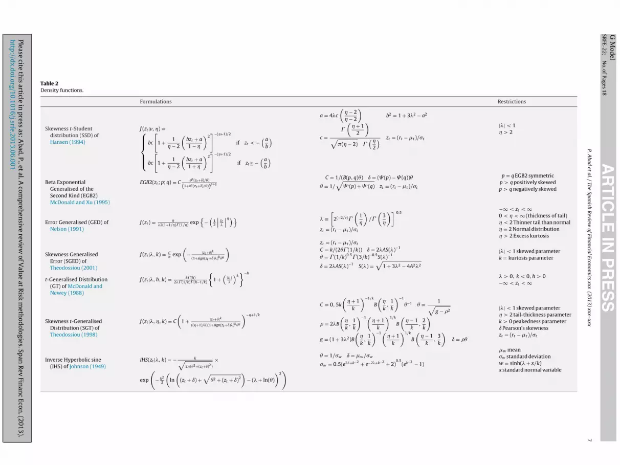
not capture the skewness of the return. Taking this into account,one direction for research in risk management involves searchingfor other distribution functions that capture these characteris-tics. In the context of VaR methodology, several density functionshave been considered: the Skewness t-Student Distribution (SSD)of Hansen (1994); Exponential Generalised Beta of the SecondKind (EGB2) of McDonald and Xu (1995); Error Generalised Dis-tribution (GED) of Nelson (1991); Skewness Error GeneralisedDistribution (SGED) of Theodossiou (2001); t-Generalised Distri-bution of McDonald and Newey (1988); Skewness t-Generaliseddistribution (SGT) of Theodossiou (1998) and Inverse HyperbolicSign (IHS) of Johnson (1949). In Table 2, we present the densityfunctions of these distributions.

In this line, some papers such as Duffie and Pan (1997) andHull and White (1998) show that a mixture of normal distributionsproduces distributions with fatter tails than a normal distributionwith the same variance.

Some applications to estimate the VaR of skewed distributionsand a mixture of normal distributions can be found in Chengand Hung (2011), Polanski and Stoja (2010), Bali and Theodossiou(2008), Bali et al. (2008), Haas et al. (2004), Zhang and Cheng (2005),Haas (2009), Ausín and Galeano (2007), Xu and Wirjanto (2010) andKuester et al. (2006).

These papers raise some important issues. First, regarding thenormal and t-Student distributions, the skewed and fat-tail dis-tributions seem to improve the fit of financial data (see Bali andTheodossiou, 2008; Bali et al., 2008; Bali and Theodossiou, 2007).Consistently, some studies found that the VaR estimate obtainedunder skewed and fat-tailed distributions provides a more accurateVaR than those obtained from a normal or t-Student distribution.For example, Cheng and Hung (2011) compared the ability to fore-cast the VaR of a normal, t-Student, SSD and GED. In this comparisonthe SSD and GED distributions provide the best results. Polanski andStoja (2010) compared the normal, t-Student, SGT and EGB2 dis-tributions and found that just the latter two distributions provideaccurate VaR estimates. Bali and Theodossiou (2007) compared anormal distribution with the SGT distribution. Again, they foundthat the SGT provided a more accurate VaR estimate. The main dis-advantage of using some skewness distribution, such as SGT, is thatthe maximisation of the likelihood function is very complicated sothat it may take a lot of computational time (see Nieto and Ruiz,2008).

Additionally, a mixture of normal distributions, t-Student distri-butions or GED distributions provided a better VaR estimate thanthe normal or t-Student distributions (see Hansen, 1994; Zhangand Cheng, 2005; Haas, 2009; Ausín and Galeano, 2007; Xu andWirjanto, 2010; Kuester et al., 2006). These studies showed that inthe context of the Parametric method, the VaR estimations obtainedwith models involving a mixture with normal distributions (andt-Student distributions) are generally quite precise.

Lastly, to handle the non-normality of the financial return Hulland White (1998) develop a new model where the user is free tochoose any probability distribution for the daily return and theparameters of the distribution are subject to an updating schemesuch as GARCH. They propose transforming the daily return into anew variable that is normally distributed. The model is appealingin that the calculation of VaR is relatively straightforward and canmake use of Riskmetrics or a similar database.

2.2.3. Higher-order conditional time-varying momentsThe traditional parametric approach for conditional VaR

assumes that the distribution of returns standardised by condi-

ew of Value at Risk methodologies. Span Rev Financ Econ. (2013).

tional means and conditional standard deviations is iid. However,there is substantial empirical evidence that the distribution offinancial returns standardised by conditional means and volatil-ity is not iid. Earlier studies also suggested that the process of

Please cite

this

article in

press

as: A

bad,

P., et

al. A

comp

rehen

sive review

of V

alue

at R

isk m

ethod

ologies. Sp

an R

ev Fin

anc

Econ.

(2013).h

ttp://d

x.doi.org/10.1016/j.srfe.2013.06.001 A

RT

ICL

E IN

PR

ES

SG

Model

SRFE-22;

N

o. of

Pages 18

P. A

bad et

al. /

The Spanish

Review

of Financial

Economics

xxx (2013)

xxx–xxx

7

Table 2Density functions.

Formulations Restrictions

Skewness t-Studentdistribution (SSD) ofHansen (1994)

f (zt |v, ) =⎧⎪⎪⎨⎪⎪⎩

bc

[1 + 1

− 2

(bzt + a

1 −

)2]−(+1)/2

if zt < −( a

b

)bc

[1 + 1

− 2

(bzt + a

1 +

)2]−(+1)/2

if zt≥ −( a

b

)

a = 4�c

( − 2 − 2

)b2 = 1 + 3�2 − a2

c =�

( + 1

2

)√

�( − 2) �(

2

) zt = (rt − �t )/�t

|�| < 1 > 2

Beta ExponentialGeneralised of theSecond Kind (EGB2)McDonald and Xu (1995)

EGB2(zt ; p; q) = C ep(zt +ı)/�)

(1+ep(zt +ı)/�))p+q

C = 1/(B(p, q)�) ı = ( (p) − (q))�

� = 1/√

′(p) + ′(q) zt = (rt − �t )/�t

p = q EGB2 symmetricp > q positively skewedp > q negatively skewed

Error Generalised (GED) ofNelson (1991)

f (zt ) = �2(1+1/)� (1/) exp

{−(

12

∣∣ zt�

∣∣)} � ≡[

2(−2/v)�

(1

)/�

(3

)]zt = (rt − �t )/�t

0.5−∞ < zt < ∞0 < < ∞ (thickness of tail) < 2 Thinner tail than normal = 2 Normal distribution > 2 Excess kurtosis

Skewness GeneralisedError (SGED) ofTheodossiou (2001)

f (zt |�, k) = C� exp

(− |zt +ı|k

(1+sign(zt +ı)�)k�k

) zt = (rt − �t )/�t

C = k/(2�� (1/k)) ı = 2�AS(�)−1

� = � (1/k)0.5� (3/k)−0.5S(�)−1

ı = 2�AS(�)−1 S(�) =√

1 + 3�2 − 4A2�2

|�| < 1 skewed parameterk = kurtosis parameter

t-Generalised Distribution(GT) of McDonald andNewey (1988)

f (zt |�, h, k) = k� (h)2�� (1/k)� (h−1/k)

{1 +(

|zt |�

)k}−h

� > 0, k < 0, h > 0−∞ < zt < ∞

Skewness t-GeneralisedDistribution (SGT) ofTheodossiou (1998)

f (zt |�, , k) = C

(1 + |zt +ı|k

((+1)/k)(1+sign(zt +ı)�)k�k

)−+1/k

C = 0, 5k

( + 1

k

)−1/k

B

(

k,

1k

)−1

�−1 � = 1√g − �2

� = 2�B

(

k,

1k

)−1( + 1

k

)1/k

B

( − 1

k,

2k

)g = (1 + 3�2)B

(

k,

1k

)−1( + 1

k

)1/k

B

( − 1

k,

3k

)ı = ��

|�| < 1 skewed parameter > 2 tail-thickness parameterk > 0 peakedness parameterı Pearson’s skewnesszt = (rt − �t )/�t

Inverse Hyperbolic sine(IHS) of Johnson (1949)

IHS(zt |�, k) = − k√2�(�2+(zt +ı)2)

×

exp

(− k2

2

(ln

((zt + ı) +

√�2 + (zt + ı)2

)− (� + ln(�)

)2)

� = 1/�w ı = �w/�w

�w = 0.5(e2�+k−2 + e−2�+k−2 + 2)0.5

(ek−2 − 1)

�w mean�w standard deviationw = sinh(� + x/k)x standard normal variable

ING ModelS

8 f Finan

naTch2

Scoabahgtanmfincraa

tstvSViwGdpfisrdc

wbfvstcrm

2

aSta

v1C

ARTICLERFE-22; No. of Pages 18

P. Abad et al. / The Spanish Review o

egative extreme returns at different quantiles may differ from onenother (Engle and Manganelli, 2004; Bali and Theodossiou, 2007).hus, given the above, some studies developed a new approach toalculate conditional VaR. This new approach considered that theigher-order conditional moments are time-varying (see Bali et al.,008; Polanski and Stoja, 2010; Ergun and Jun, 2010).

Bali et al. (2008) introduced a new method based on theGT with time-varying parameters. They allowed higher-orderonditional moment parameters of the SGT density to dependn the past information set and hence relax the conventionalssumption in the conditional VaR calculation that the distri-ution of standardised returns is iid. Following Hansen (1994)nd Jondeau and Rockinger (2003), they modelled the conditionaligh-order moment parameters of the SGT density as an autore-ressive process. The maximum likelihood estimates show thathe time-varying conditional volatility, skewness, tail-thickness,nd peakedness parameters of the SGT density are statistically sig-ificant. In addition, they found that the conditional SGT-GARCHodels with time-varying skewness and kurtosis provided a better

t or returns than the SGT-GARCH models with constant skew-ess and kurtosis. In their paper, they applied this new approach toalculate the VaR. The in-sample and out-of-sample performanceesults indicated that the conditional SGT-GARCH approach withutoregressive conditional skewness and kurtosis provided veryccurate and robust estimates of the actual VaR thresholds.

In a similar study, Ergun and Jun (2010) considered the SSD dis-ribution, which they called the ARCD model, with a time-varyingkewness parameter. They found that the GARCH-based modelshat take conditional skewness and kurtosis into account pro-ided an accurate VaR estimate. Along this same line, Polanski andtoja (2010) proposed a simple approach to forecast a portfolioaR. They employed the Gram-Charlier expansion (GCE) augment-

ng the standard normal distribution with the first four moments,hich are allowed to vary over time. The key idea was to employ theCE of the standard normal density to approximate the probabilityistribution of daily returns in terms of cumulants.8 This approachrovides a flexible tool for modelling the empirical distribution ofnancial data, which, in addition to volatility, exhibits time-varyingkewness and leptokurtosis. This method provides accurate andobust estimates of the realised VaR. Despite its simplicity, theirataset outperformed other estimates that were generated by bothonstant and time-varying higher-moment models.

All previously mentioned papers compared their VaR estimatesith the results obtained by assuming skewed and fat-tail distri-

utions with constant asymmetric and kurtosis parameters. Theyound that the accuracy of the VaR estimates improved when time-arying asymmetric and kurtosis parameters are considered. Thesetudies suggest that within the context of the Parametric method,echniques that model the dynamic performance of the high-orderonditional moments (asymmetry and kurtosis) provide betteresults than those considering functions with constant high-orderoments.

.3. Semi-parametric methods

The Semi-parametric methods combine the Non-parametricpproach with the Parametric approach. The most importantemi-parametric methods are Volatility-weight Historical Simula-

Please cite this article in press as: Abad, P., et al. A comprehensive revihttp://dx.doi.org/10.1016/j.srfe.2013.06.001

ion, Filtered Historical Simulation (FHS), CaViaR method and thepproach based on Extreme Value Theory.

8 Although in different contexts, approximating the distribution of asset returnsia the GCE has been previously employed in the literature (e.g., Jarrow and Rudd,982; Baillie and Bollerslev, 1992; Jondeau and Rockinger, 2001; Leon et al., 2005;hristoffersen and Diebold, 2006).

PRESScial Economics xxx (2013) xxx–xxx

2.3.1. Volatility-weight historical simulationTraditional Historical Simulation does not take any recent

changes in volatility into account. Thus, Hull and White (1998)proposed a new approach that combines the benefit of HistoricalSimulation with volatility models. The basic idea of this approachis to update the return information to take into account the recentchanges in volatility.

Let rt,i be the historical return on asset i on day t in our historicalsample, �t,i be the forecast of the volatility9 of the return on asset ifor day t made at the end of t − 1, and �T,i be our most recent forecastof the volatility of asset i. Then, we replace the return in our dataset, rt,i, with volatility-adjusted returns, as given by:

r∗t,i = �T,irt,i

�t,i(10)

According to this new approach, the VaR(˛) is the quantile ofthe empirical distribution of the volatility adjusted return (r∗

t,i).

This approach directly takes into account the volatility changes,whereas the Historical Simulation approach ignores them. Further-more, this method produces a risk estimate that is appropriatelysensitive to current volatility estimates. The empirical evidencepresented by Hull and White (1998) indicates that this approachproduces a VaR estimate superior to that of the Historical Simula-tion approach.

2.3.2. Filtered Historical SimulationFiltered Historical Simulation was proposed by Barone-Adesi

et al. (1999). This method combines the benefits of HistoricalSimulation with the power and flexibility of conditional volatilitymodels.

Suppose we use Filtered Historical Simulation to estimate theVaR of a single-asset portfolio over a 1-day holding period. In imple-menting this method, the first step is to fit a conditional volatilitymodel to our portfolio return data. Barone-Adesi et al. (1999) rec-ommended an asymmetric GARCH model. The realised returnsare then standardised by dividing each one by the correspondingvolatility, zt = (εt/�t). These standardised returns should be inde-pendent and identically distributed and therefore be suitable forHistorical Simulation. The third step consists of bootstrapping alarge number L of drawings from the above sample set of standard-ised returns.

Assuming a 1-day VaR holding period, the third stage involvesbootstrapping from our data set of standardised returns: we take alarge number of drawings from this data set, which we now treatas a sample, replacing each one after it has been drawn and mul-tiplying each such random drawing by the volatility forecast 1 dayahead:

rt = �t + z∗�t+1 (11)

where z* is the simulated standardised return. If we take M draw-ings, we therefore obtain a sample of M simulated returns. Withthis approach, the VaR(˛) is the ˛% quantile of the simulated returnsample.

Recent empirical evidence shows that this approach works quitewell in estimating VaR (see Barone-Adesi and Giannopoulos, 2001;Barone-Adesi et al., 2002; Zenti and Pallotta, 2001; Pritsker, 2001;Giannopoulos and Tunaru, 2005). As for other methods, Zikovicand Aktan (2009), Angelidis et al. (2007), Kuester et al. (2006) andMarimoutou et al. (2009) provide evidence that this method is thebest for estimating the VaR. However, other papers indicate that

ew of Value at Risk methodologies. Span Rev Financ Econ. (2013).

this approach is not better than any other (see Nozari et al., 2010;Alonso and Arcos, 2006).

9 To estimate the volatility of the returns, several volatility models can be used.Hull and White (1998) proposed a GARCH model and the EWMA model.

ING ModelS

f Finan

2

gepvlCdnoam

vbtc

V

wnˇoaiss

V

fi

-

-

ta((

V

u

ssentC(Lmd

s

ARTICLERFE-22; No. of Pages 18

P. Abad et al. / The Spanish Review o

.3.3. CAViaR modelEngle and Manganelli (2004) proposed a conditional autore-

ressive specification for VaR. This approach is based on a quantilestimation. Instead of modelling the entire distribution, they pro-osed directly modelling the quantile. The empirical fact that theolatilities of stock market returns cluster over time may be trans-ated quantitatively in that their distribution is autocorrelated.onsequently, the VaR, which is tightly linked to the standardeviation of the distribution, must exhibit similar behaviour. Aatural way to formalise this characteristic is to use some typef autoregressive specification. Thus, they proposed a conditionalutoregressive quantile specification that they called the CAViaRodel.Let rt be a vector of time t observable financial return and ˇ˛ a p-

ector of unknown parameters. Finally, let VaRt(ˇ) ≡ VaRt(rt−1, ˇ˛)e the quantile of the distribution of the portfolio return formed atime t − 1, where we suppress the subscript from ˇ˛ for notationalonvenience.

A generic CAViaR specification might be the following:

aRt(ˇ) = ˇ0 +q∑

i=1

ˇiVaRt−i(ˇ) +r∑

j=1

ˇjl(xt−j) (12)

here p = q + r + 1 is the dimension of and l is a function of a finiteumber of lagged observable values. The autoregressive termsiVaRt−i (ˇ) i = 1,. . ., q ensure that the quantile changes “smoothly”ver time. The role of l(rt − 1) is to link VaRt(ˇ) to observable vari-bles that belong to the information set. A natural choice for xt − 1s lagged returns. The advantage of this method is that it makes nopecific distributional assumption on the return of the asset. Theyuggested that the first order is sufficient for practical use:

aRt(ˇ) = ˇ0 + ˇ1VaRt−1(ˇ) + ˇ2l(rt−i, VaRt−1) (13)

In the context of CAViaR model, different autoregressive speci-cations can be considered

Symmetric absolute value (SAV):

VaRt(ˇ) = ˇ0 + ˇ1VaRt−1(ˇ) + ˇ2|rt−1| (14)

Indirect GARCH(1,1) (IG):

VaRt(ˇ) = (ˇ0 + ˇ1VaR2t−1(ˇ) + ˇ2(rt−1)2)

1/2(15)

In these two models the effects of the extreme returns andhe variance on the VaR measure are modelled symmetrically. Toccount for financial market asymmetry, via the leverage effectBlack, 1976), the SAV model was extended in Engle and Manganelli2004) to asymmetric slope (AS):

aRt(ˇ) = ˇ0 + ˇ1VaRt−1(ˇ) + ˇ2(rt−1)+ + ˇ3(rt−1))− (16)

In this representation, (r)+ = max(rt,0) and (rt)− = −min(rt,0) aresed as the functions.

The parameters of the CAViaR models are estimated by regres-ion quantiles, as introduced by Koenker and Basset (1978). Theyhowed how to extend the notion of a sample quantile to a lin-ar regression model. In order to capture leverage effects and otheronlinear characteristics of the financial return, some extensions ofhe CAViaR model have been proposed. Yu et al. (2010) extend theAViaR model to include the Threshold GARCH (TGARCH) modelan extension of the double threshold ARCH (DTARCH) of Li andi (1996)) and a mixture (an extension of Wong and Li (2001)’s

Please cite this article in press as: Abad, P., et al. A comprehensive revihttp://dx.doi.org/10.1016/j.srfe.2013.06.001

ixture ARCH). Recently, Chen et al. (2011) proposed a non-linearynamic quantile family as a natural extension of the AS model.

Although empirical literature on CAViaR method is not exten-ive, the results seem to indicate that the CAViaR model proposed

PRESScial Economics xxx (2013) xxx–xxx 9

by Engle and Manganelli (2004) fails to provide accurate VaR esti-mate although it may provide accurate VaR estimates in a stableperiod (see Bao et al., 2006; Polanski and Stoja, 2009). However,some recent extensions of the CaViaR model such as those proposedby Gerlach et al. (2011) and Yu et al. (2010) work pretty well in esti-mating VaR. As in the case of the Parametric method, it appears thatwhen use is made of an asymmetric version of the CaViaR modelthe VaR estimate notably improves. The paper of Sener et al. (2012)supports this hypothesis. In a comparison of several CaViaR models(asymmetric and symmetric) they find that the asymmetric CaViaRmodel outperforms the result from the standard CaViaR model.Gerlach et al. (2011) compared three CAViaR models (SAV, AS andThreshold CAViaR) with the Parametric method using differentvolatility GARCH family models (GARCH-Normal, GARCH-Student-t, GJR-GARCH, IGARCH, Riskmetric). At the 1% confidence level, theThreshold CAViaR model performs better than any other.

2.3.4. Extreme Value TheoryThe Extreme Value Theory (EVT) approach focuses on the

limiting distribution of extreme returns observed over a long timeperiod, which is essentially independent of the distribution of thereturns themselves. The two main models for EVT are (1) theblock maxima models (BM) (McNeil, 1998) and (2) the peaks-over-threshold model (POT). The second is generally considered to bethe most useful for practical applications due to the more efficientuse of the data at extreme values. In the POT models, there are twotypes of analysis: the Semi-parametric models built around the Hillestimator and its relatives (Beirlant et al., 1996; Danielsson et al.,1998) and the fully Parametric models based on the GeneralisedPareto distribution (Embrechts et al., 1999). In the coming sectionseach one of these approaches is described.

2.3.4.1. Block Maxima Models (BMM). This approach involves split-ting the temporal horizon into blocks or sections, taking intoaccount the maximum values in each period. These selected obser-vations form extreme events, also called a maximum block.

The fundamental BMM concept shows how to accurately choosethe length period, n, and the data block within that length. Forvalues greater than n, the BMM provides a sequence of maximumblocks Mn,1,. . ., Mn,m that can be adjusted by a generalised distri-bution of extreme values (GEV). The maximum loss within a groupof n data is defined as Mn = max(X1, X2,. . ., Xn).

For a group of identically distributed observations, the distribu-tion function of Mn is represented as:

P(Mn ≤ x) = P(X1 ≤ x, . . ., Xn ≤ x) =n∏

i=1

F(x) = Fn(x) (17)

The asymptotic approach for Fn(x) is based on the maximumstandardised value

Zn = Mn − �n

�n(18)

where �n and �n are the location and scale parameters, respec-tively. The theorem of Fisher and Tippet establishes that if Zn

converges to a non-degenerated distribution, this distribution is thegeneralised distribution of the extreme values (GEV). The algebraicexpression for such a generalised distribution is as follows:

H�,�,� (x) ={

exp (−1 + �(x − �)/�)−1/� � /= 0 and (1 + �(x − �)/�) > 0

exp(−e−x) � = 0(19)

where � > 0, −∞ < � < ∞, and −∞ < � < ∞. The parameter � is known

ew of Value at Risk methodologies. Span Rev Financ Econ. (2013).

as the shape parameter of the GEV distribution, and = �−1 is theindex of the tail distribution, H. The prior distribution is actually ageneralisation of the three types of distributions, depending on thevalue taken by �: Gumbel type I family (� = 0), Fréchet type II family

ING ModelS

1 f Finan

(at

V

tv

nsr

2edtttt

ARTICLERFE-22; No. of Pages 18

0 P. Abad et al. / The Spanish Review o

� > 0) and Weibull type III family (� < 0). The �, � and � parametersre estimated using maximum likelihood. The VaR expression forhe Gumbel and Fréchet distribution is as follows:

aR ={

�n − �n

�n(1 − (−n ln(˛))−�n ) to � > 0 (Fré chet)

�n − �n ln(−n ln(˛)) to � = 0 (Gumbel)(20)

In most situations, the blocks are selected in such a way thatheir length matches a year interval and n is the number of obser-ations within that year period.

This method has been commonly used in hydrology and engi-eering applications but is not very suitable for financial timeeries due to the cluster phenomenon largely observed in financialeturns.

.3.4.2. Peaks over threshold models (POT). The POT model is gen-rally considered to be the most useful for practical applicationsue to the more efficient use of the data for the extreme values. Inhis model, we can distinguish between two types of analysis: (a)he fully Parametric models based on the Generalised Pareto dis-ribution (GPD) and (b) the Semi-parametric models built aroundhe Hill estimator.

(a) Generalised Pareto DistributionAmong the random variables representing financial returns

(r1, r2, r3,. . ., rn), we choose a low threshold u and examine allvalues (y) exceeding u: (y1, y2, y3, . . ., yNu ), where yi = ri − u andNu are the number of sample data greater than u. The distribu-tion of excess losses over the threshold u is defined as:

Fu(y) = P(r − u < y|r > u) = F(y + u) − F(u)1 − F(u)

(21)

Assuming that for a certain u, the distribution of excesslosses above the threshold is a Generalised Pareto Distribu-tion, Gk,�(y) = 1 − [1 + (k/�)y]−1/k, the distribution function ofreturns is given by:

F(r) = F(y + u) = [1 − F(u)]Gk,�(y) + F(u) (22)

To construct a tail estimator from this expression, the onlyadditional element we need is an estimation of F(u). For thispurpose, we take the obvious empirical estimator (u − Nu)/u.We then use the historical simulation method. Introducing thehistorical simulation estimate of F(u) and setting r = y + u in theequation, we arrive at the tail estimator

F(r) = 1 − Nu

n

[1 + k

�(r − u)

]−1/k

r > u (23)

For a given probability > F(u), the VaR estimate is calculatedby inverting the tail estimation formula to obtain

VaR(˛) = u + �

k

[[n

Nu(1 − ˛)

]−k

− 1

](24)

None of the previous Extreme Value Theory-based meth-ods for quantile estimation yield VaR estimates that reflectthe current volatility background. These methods are calledUnconditional Extreme Value Theory methods. Given the condi-tional heteroscedasticity characteristic of most financial data,McNeil and Frey (2000) proposed a new methodology to esti-mate the VaR that combines the Extreme Value Theory with

Please cite this article in press as: Abad, P., et al. A comprehensive revihttp://dx.doi.org/10.1016/j.srfe.2013.06.001

volatility models, known as the Conditional Extreme Value The-ory. These authors proposed GARCH models to estimate thecurrent volatility and Extreme Value Theory to estimate thedistributions tails of the GARCH model shocks.

PRESScial Economics xxx (2013) xxx–xxx

If the financial returns are a strictly stationary time series andε follows a Generalised Pareto Distribution, denoted by Gk,� (ε),the conditional quantile of the returns can be estimated as

VaR(˛) = � + �tG−1k,�

(˛) (25)

where �2t represents the conditional variance of the financial

returns and G−1k,�

(˛) is the quantile of the GPD, which can becalculated as:

G−1k,�

(˛) = u + �

k

[[n

Nu(1 − ˛)

]−k

− 1

](26)

(b) Hill estimatorThe parameter that collects the features of the tail distribu-

tion is the tail index, = �−1. Hill proposed a definition of thetail index as follows:

H =[

1u

(u∑

i=1

log(ri) − log ru+1

)]−1

(27)

where ru represents the threshold return and u is the num-ber of observations equal to or less than the threshold return.Thus, the Hill estimator is the mean of the most extreme uobservations minus u + 1 observations (ru + 1). Additionally, theassociated quantile estimator is (see Danielsson and de Vries,2000):

VaR(˛) = ru+1

(1 − ˛

u/n

)−1/

(28)

The problem posed by this estimator is the lack of any analyticalmeans to choose the threshold value of u in an optimum manner.Hence, as an alternative, the procedure involves using the featureknown as Hill graphics. Different values of the Hill index are cal-culated for different u values; the Hill estimator values becomerepresented in a chart or graphic based on u, and the u value isselected from the region where the Hill estimators are relativelystable (Hill chart leaning almost horizontally). The underlying intu-itive idea posed in the Hill chart is that as u increases, the estimatorvariance decreases, and thus, the bias is increased. Therefore, theability to foresee a balance between both trends is likely. When thislevel is reached, the estimator remains constant.

Existing literature on EVT models to calculate VaR is abundant.Regarding BMM, Silva and Melo (2003) considered different maxi-mum block widths, with results suggesting that the extreme valuemethod of estimating the VaR is a more conservative approachfor determining the capital requirements than traditional meth-ods. Byström (2004) applied both unconditional and conditionalEVT models to the management of extreme market risks in thestock market and found that conditional EVT models provided par-ticularly accurate VaR measures. In addition, a comparison withtraditional Parametric (GARCH) approaches to calculate the VaRdemonstrated EVT as being the superior approach for both standardand more extreme VaR quantiles. Bekiros and Georgoutsos (2005)conducted a comparative evaluation of the predictive performanceof various VaR models, with a special emphasis on two method-ologies related to the EVT, POT and BM. Their results reinforcedprevious results and demonstrated that some “traditional” meth-ods might yield similar results at conventional confidence levels butthat the EVT methodology produces the most accurate forecasts ofextreme losses at very high confidence levels. Tolikas et al. (2007)compared EVT with traditional measures (Parametric method, HS

ew of Value at Risk methodologies. Span Rev Financ Econ. (2013).

and Monte Carlo) and agreed with Bekiros and Georgoutsos (2005)on the outperformance of the EVT methods compared with the rest,especially at very high confidence levels. The only model that hada performance comparable with that of the EVT is the HS model.

ING ModelS

f Finan

tteaabbVaAEV

wtbGaa(c(wdtatupEbEmdmee

tB

2

tuVsVs

rcvfircuztsu

mbt

totically distributed �2 (2), and the LRind statistic is the likelihoodratio statistic for the hypothesis of serial independence againstfirst-order Markov dependence.10

10 The LRind statistic is LRind = 2 [log LA − log L0] and has an asymptotic �2 (1)

ARTICLERFE-22; No. of Pages 18

P. Abad et al. / The Spanish Review o

Some papers showed that unconditional EVT works better thanhe traditional HS or Parametric approaches when a normal dis-ribution for returns is assumed and a EWMA model is used tostimate the conditional volatility of the return (see Danielssonnd de Vries, 2000). However, the unconditional version of thispproach has not been profusely used in the VaR estimationecause such an approach has been overwhelmingly dominatedy the conditional EVT (see McNeil and Frey, 2000; Ze-To, 2008;elayoudoum et al., 2009; Abad and Benito, 2013). Recent compar-tive studies of VaR models, such as Nozari et al. (2010), Zikovic andktan (2009) and Genc ay and Selc uk (2004), show that conditionalVT approaches perform the best with respect to forecasting theaR.

Within the POT models, an environment has emerged inhich some studies have proposed some improvements on cer-

ain aspects. For example, Brooks et al. (2005) calculated the VaRy a semi-nonparametric bootstrap using unconditional density, aARCH (1,1) model and EVT. They proposed a Semi-nonparametricpproach using a GPD, and this method was shown to generate

more accurate VaR than any other method. Marimoutou et al.2009) used different models and confirmed that the filtering pro-ess was important for obtaining better results. Ren and Giles2007) introduced the media excessive function concept as a neway to choose the threshold. Ze-To (2008) developed a new con-itional EVT-based model combined with the GARCH-Jump modelo forecast extreme risks. He utilised the GARCH-Jump model tosymmetrically provide the past realisation of jump innovation tohe future volatility of the return distribution as feedback and alsosed the EVT to model the tail distribution of the GARCH-Jump-rocessed residuals. The model is compared with unconditionalVT and conditional EVT-GARCH models under different distri-utions, normal and t-Student. He shows that the conditionalVT-GARCH-Jump model outperforms the GARCH and GARCH-todels. Chan and Gray (2006) proposed a model that accommo-

ates autoregression and weekly seasonals in both the conditionalean and conditional volatility of the returns as well as leverage

ffects via an EGARCH specification. In addition, EVT is adopted toxplicitly model the tails of the return distribution.

Finally, concerning the Hill index, some authors used the men-ioned estimator, such as Bao et al. (2006), whereas others such ashattacharyya and Ritolia (2008) used a modified Hill estimator.

.3.5. Monte CarloThe simplest Monte Carlo procedure to estimate the VaR on date

on a one-day horizon at a 99% significance level consists of sim-lating N draws from the distribution of returns on date t + 1. TheaR at a 99% level is estimated by reading off element N/100 afterorting the N different draws from the one-day returns, i.e., theaR estimate is estimated empirically as the VaR quantile of theimulated distribution of returns.

However, applying simulations to a dynamic model of risk factoreturns that capture path dependent behaviour, such as volatilitylustering, and the essential non-normal features of their multi-ariate conditional distributions is important. With regard to therst of these, one of the most important features of high-frequencyeturns is that volatility tends to come in clusters. In this case, wean obtain the GARCH variance estimate at time t( �t) using the sim-lated returns in the previous simulation and set r1 = �tzt , wheret is a simulation from a standard normal variable. With regardo the second item, we can model the interdependence using thetandard multivariate normal or t-Student distribution or use cop-las instead of correlation as the dependent metric.

Please cite this article in press as: Abad, P., et al. A comprehensive revihttp://dx.doi.org/10.1016/j.srfe.2013.06.001

Monte Carlo is an interesting technique that can be used to esti-ate the VaR for non-linear portfolios (see Estrella et al., 1994)

ecause it requires no simplifying assumptions about the joint dis-ribution of the underlying data. However, it involves considerable

PRESScial Economics xxx (2013) xxx–xxx 11

computational expenses. This cost has been a barrier limiting itsapplication into real-world risk containment problems. Srinivasanand Shah (2001) proposed alternative algorithms that require mod-est computational costs and, Antonelli and Iovino (2002) proposeda methodology that improves the computational efficiency of theMonte Carlo simulation approach to VaR estimates.

Finally, the evidence shown in the studies on the comparisonof VaR methodologies agree with the greater accuracy of the VaRestimations achieved by methods other than Monte Carlo (see Abadand Benito, 2013; Huang, 2009; Tolikas et al., 2007; Bao et al., 2006).

To sum up, in this section we have reviewed some of the mostimportant VaR methodologies, from the standard models to themore recent approaches. From a theoretical point of view, all ofthese approaches show advantages and disadvantages. In Table 3,we resume these advantages and disadvantages. In the next sec-tions, we will review the results obtained for these methodologiesfrom a practical point of view.

3. Back-testing VaR methodologies

Many authors are concerned about the adequacy of the VaRmeasures, especially when they compare several methods. Papers,which compare the VaR methodologies commonly use two alter-native approaches: the basis of the statistical accuracy tests and/orloss functions. As to the first approach, several procedures based onstatistical hypothesis testing have been proposed in the literatureand authors usually select one or more tests to evaluate the accu-racy of VaR models and compare them. The standard tests aboutthe accuracy VaR models are: (i) unconditional and conditionalcoverage tests; (ii) the back-testing criterion and (iii) the dynamicquantile test. To implement all these tests an exception indicatormust be defined. This indicator is calculated as follows:

It+1 ={

1 if rt+1 < VaR(˛)

0 if rt+1 > VaR(˛)(29)

Kupiec (1995) shows that assuming the probability of an excep-tion is constant, then the number of exceptions x =

∑It+1 follows

a binomial distribution B(N, ˛), where N is the number of observa-tions. An accurate VaR(˛) measure should produce an unconditionalcoverage ( ˆ =

∑It+1/N) equal to percent. The unconditional cov-

erage test has as a null hypothesis ˆ = ˛, with a likelihood ratiostatistic:

LRUC = 2[log(�˛x(1 − �˛)N−x) − log(˛x(1 − ˛)N−x)] (30)

which follows an asymptotic �2 (1) distribution.Christoffersen (1998) developed a conditional coverage test. This

jointly examines whether the percentage of exceptions is statis-tically equal to the one expected and the serial independence ofIt + 1. He proposed an independence test, which aimed to reject VaRmodels with clustered violations. The likelihood ratio statistic ofthe conditional coverage test is LRcc = LRuc + LRind, which is asymp-

ew of Value at Risk methodologies. Span Rev Financ Econ. (2013).

distribution. The likelihood function under the alternative hypothesis is LA =(1 − �01)N00 �N01

01 (1 − �11)N10 �N1111 where Nij denotes the number of observations in

state j after having been in state i in the previous period, �01 = N01/(N00 + N01)and �11 = N11/(N10 + N11). The likelihood function under the null hypothesis is(�01 = �11 = � = (N11 + N01)/N) is L0 = (1 − �)N00+N01 �N01+N11 .

ARTICLE IN PRESSG ModelSRFE-22; No. of Pages 18

12 P. Abad et al. / The Spanish Review of Financial Economics xxx (2013) xxx–xxx

Table 3Advantages and disadvantages of VaR approaches.

Advantages Disadvantages

Non Parametric approach (HS)Minimal assumptions made about the error distribution,nor the exact form of the dynamic specifications

• Not making strong assumptionsabout the distribution of the returnsportfolio, they can accommodate widetails, skewness and any othernon-normal features.• It is very easy to implement.

• Its results are completely dependenton the data set.• It is sometimes slow to reflect majorevents.• It is only allows us to estimate VaR atdiscrete confidence intervalsdetermined by the size of our data set.

Parametric approachMakes a full parametric distributional and model formassumption. For example AGARCH model with Gaussianerrors

• Its ease of implementation when anormal or Student-t distributions isassumed.

• It ignores leptokurtosis and skewnesswhen a normal distribution is assumed.• Difficulties of implementation when askewed distributions is assumeda.

RiskmetricsA kind of parametric approach

• Its ease of implementation can becalculated using a spreadsheet.

• It assumes normality of returnignoring fat tails, skewness, etc.• This model lack non linear propertywhich is a significant of the financialreturn.

Semiparametric approachSome assumptions are made, eitherabout the error distribution, itsextremes, or the model dynamics

Filter HistoricalSimulation

• This approach retains thenonparametric advantage (HS) and atthe same time addresses some of HS’sinherent problems, i.e. FHS takevolatility background into account.

• Its results slightly dependent on thedata set.

ETV • Capture curtosis and changes involatility (conditional ETV).

• It depends on the extreme returndistribution assumption.• Its results depend on the extremedata set.

CaViaR • It makes no specific distributionalassumption on the return of the asset.• It captures non linear characteristicsof the financial returns.

• Difficulties of implementation.

Monte Carlo • The large number of scenariosgenerated provide a more reliable andcomprehensive measure of risk thananalytical method.• It captures convexity of non linearinstruments and changes in volatilityand time.

• Its reliance on the stochastic processspecified or historical data selected togenerate estimations of the final valueof the portfolio and hence of the VaR.• It involves considerablecomputational expenses.

kage,s say ts ot of c

t

Z

w

Mu˝t

I

a˝b

patis(OtC

a In addition, as the skewness distributions are not included in any statistical paceveral program language can be used: MATLAB, R, GAUSS, etc. It is in this sense weeveral skewed distributions, such as, SGT is very complicated so that it can take a l

A similar test for the significance of the departure of ˆ from ishe back-testing criterion statistic:

= (N�˛ − N˛)√N˛(1 − ˛)

(31)

hich follows an asymptotic N(0,1) distribution.Finally, the Dynamic Quantile (DQ) test proposed by Engle and

anganelli (2004) examines whether the exception indicator isncorrelated with any variable that belongs to the information sett−1 available when the VaR was calculated. This is a Wald test of

he hypothesis that all slopes in the regression model

t = ˇ0 +p∑

i=1

ˇiIt−1 +q∑

j=i

�jXj + εt (32)

re equal to zero, where Xj are explanatory variables contained int−1.VaR(˛) is usually an explanatory variable to test if the proba-

ility of an exception depends on the level of the VaR.The tests described above are based on the assumption that the

arameters of the models fitted to estimate the VaR are known,lthough they are estimations. Escanciano and Olmo (2010) showhat the use of standard unconditional and independence backtest-ng procedures can be misleading. They propose a correction of thetandard backtesting procedures. Additionally, Escanciano and Pei

Please cite this article in press as: Abad, P., et al. A comprehensive revihttp://dx.doi.org/10.1016/j.srfe.2013.06.001

2012) propose correction when VaR is estimated with HS or FHS.n a different route, Baysal and Staum (2008) provide a test on

he coverage of confidence regions and intervals involving VaR andonditional VaR.

the user of this methodology have to program their code of estimation To do that,hat the implementation is difficult. As the maximisation of the likelihood based onomputational time.

The second approach is based on the comparison of loss func-tions. Some authors compare the VaR methodologies by evaluatingthe magnitude of the losses experienced when an exception occursin the models. The “magnitude loss function” that addresses themagnitude of the exceptions was developed by Lopez (1998, 1999).It deals with a specific concern expressed by the Basel Committeeon Banking Supervision, which noted that the magnitude, as wellas the number of VaR exceptions is a matter of regulatory con-cern. Furthermore, the loss function usually examines the distancebetween the observed returns and the forecasted VaR(�) values ifan exception occurs.

Lopez (1999) proposed different loss functions:

lft+1 ={

z(rt+1, VaR(˛)) if rt+1 < VaR(˛)

0 if rt+1 > VaR(˛)(33)

where the VaR measure is penalised with the exception indi-cator (z(.) = 1), the exception indicator plus the square distance(z(.) = 1 + (rt + 1 − VaR(˛))2 or using weight (z(rt + 1,VaR(˛)x) = k,where x, being the number of exceptions, is divided into severalzones and k is a constant which depends on zone) based on whatregulators consider to be a minimum capital requirement reflect-ing their concerns regarding prudent capital standards and modelaccuracy.

ew of Value at Risk methodologies. Span Rev Financ Econ. (2013).

More recently, other authors have proposed loss func-tion alternatives, such as Abad and Benito (2013) whoconsider z(.) = (rt + 1 − VaR(˛))2and z(.) = |rt + 1 − VaR(˛)| orCaporin (2008) who proposes z(.) =

∣∣1 −∣∣rt+1/VaR(˛)

∣∣∣∣ and

ING ModelS

f Finan

zm

imBu(

lit

4

Hpwctiiamtctp

VtTeoCcwti

rwHpnop

Bsmmr

ttp2i

bb(e

ARTICLERFE-22; No. of Pages 18

P. Abad et al. / The Spanish Review o

(.) = ((|rt+1| − |VaR(˛)|)2/|VaR(˛)|). Caporin (2008) also designs aeasure of the opportunity cost.In this second approach, the best VaR model is that which min-

mises the loss function. In order to know which approach providesinimum losses, different tests can be used. For instance Abad and

enito (2013) use a non-parametric test while Sener et al. (2012)se the Diebold and Mariano (1995) test as well as that of White2000).

Another alternative to compare VaR models is to evaluate theoss in a set of hypothetical extreme market scenarios (stress test-ng). Linsmeier and Pearson (2000) discuss the advantages of stressesting.

. Comparison of VaR methods

Empirical literature on VaR methodology is quite extensive.owever, there are not many papers dedicated to comparing theerformance of a large range of VaR methodologies. In Table 4,e resume 24 comparison papers. Basically, the methodologies

ompared in these papers are HS (16 papers), FHS (8 papers),he Parametric method under different distributions (22 papersncluded the normal, 13 papers include t-Student and just 5 papersnclude any kind of skewness distribution) and the EVT basedpproach (18 papers). Only a few of these studies include otherethods, such as the Monte Carlo (5 papers), CaViaR (5 papers) and

he Non-Parametric density estimation methods (2 papers) in theiromparisons. For each article, we marked the methods included inhe comparative exercise with a cross and shaded the method thatrovides the best VaR estimations.

The approach based on the EVT is the best for estimating theaR in 83.3% of the cases in which this method is included in

he comparison, followed closely by FHS, with 62.5% of the cases.his percentage increases to 75.0% if we consider that the differ-nces between ETV and FHS are almost imperceptible in the paperf Giamouridis and Ntoula (2009), as the authors underline. TheaViaR method ranks third. This approach is the best in 3 out of 5omparison papers (it represents a percentage of success of 60%,hich is quite high). However, we must remark that only in one of

hese 3 papers, ETV is included in the comparison and FHS is notncluded in any of them.

The worst results are obtained by HS, Monte Carlo and Riskmet-ics. None of those methodologies rank best in the comparisonshere they are included. Furthermore, in many of these papersS and Riskmetrics perform worst in estimating VaR. A similarercentage of success is obtained by Parametric method under aormal distribution. Only in 2 out of 18 papers, does this method-logy rank best in the comparison. It seems clear that the newroposals to estimate VaR have outperformed the traditional ones.

Taking this into account, we highlight the results obtained byerkowitz and O’Brien (2002). In this paper the authors compareome internal VaR models used by banks with a parametric GARCHodel estimated under normality. They find that the bank VaRodels are not better than a simple parametric GARCH model. It

eveals that internal models work very poorly in estimating VaR.The results obtained by the Parametric method should be

aken into account when the conditional high-order moments areime-varying. The two papers that include this method in the com-arison obtained a 100% outcome success (see Ergun and Jun,010; Polanski and Stoja, 2010). However, only one of these papers

ncluded EVT in the comparison (Ergun and Jun, 2010).Although not shown in Table 4, the VaR estimations obtained

Please cite this article in press as: Abad, P., et al. A comprehensive revihttp://dx.doi.org/10.1016/j.srfe.2013.06.001

y the Parametric method with asymmetric and leptokurtic distri-utions and in a mixed-distribution context are also quite accuratesee Abad and Benito, 2013; Bali and Theodossiou, 2007, 2008; Balit al., 2008; Chen et al., 2011; Polanski and Stoja, 2010). However

PRESScial Economics xxx (2013) xxx–xxx 13

this method does not seem to be superior to EVT and FHS (Kuesteret al., 2006; Cifter and Özün, 2007; Angelidis et al., 2007). Never-theless, there are not many papers including these three methodsin their comparison. In this line, some recent extensions of theCaViaR method seem to perform quite well, such as those pro-posed by Yu et al. (2010) and Gerlach et al. (2011). This last papercompared three CAViaR models (SAV, AS and Threshold CAViaR)with the Parametric model under some distributions (GARCH-N,GARCH-t, GJR-GARCH, IGARCH, Riskmetric). They find that at 1%confidence level, the Threshold CAViaR model performs better thanthe Parametric models considered. Sener et al. (2012) carried out acomparison of a large set of VaR methodologies: HS, Monte Carlo,EVT, Riskmetrics, Parametric method under normal distributionand four CaViaR models (symmetric and asymmetric). They findthat the asymmetric CaViaR model joined to the Parametric modelwith an EGARCH model for the volatility performs the best in esti-mating VaR. Abad and Benito (2013), in a comparison of a largerange of VaR approaches that include EVT, find that the Parametricmethod under an asymmetric specification for conditional volatil-ity and t-Student innovations performs the best in forecasting VaR.Both papers highlight the importance of capturing the asymmetryin volatility. Sener et al. (2012) state that the performance of VaRmethods does not depend entirely on whether they are parametric,non-parametric, semi-parametric or hybrid but rather on whetherthey can model the asymmetry of the underlying data effectivelyor not.

In Table 5, we reconsider the papers of Table 4 to show whichapproach they use to compare VaR models. Most of the papers (62%)evaluate the performance of VaR models on the basis of the fore-casting accuracy. To do that not all of them used a statistical test.There is a significant percentage (25%) comparing the percentageof exceptions with that expected without using any statistical test.38% of the papers in our sample consider that both the number ofexceptions and their size are important and include both dimen-sions in their comparison.

Although there are not many articles dedicated to the com-parison of a wide range of VaR methodologies, the existing onesoffer quite conclusive results. These results show that the approachbased on the EVT and FHS is the best method to estimate the VaR.We also note that VaR estimates obtained by some asymmetricextensions of CaViaR method and the Parametric method under theskewed and fat-tail distributions lead to promising results, espe-cially when the assumption that the standardised returns is iid isabandoned and the conditional high-order moments are consid-ered to be time-varying.

5. Some important topics of VaR methodology

As we stated in the introduction, VaR is by far the leading mea-sure of portfolio risk in use in major commercial banks and financialinstitutions. However, this measurement is not exempt from crit-icism. Some researchers have remarked that VaR is not a coherentmarket measure (see Artzner et al., 1999). These authors define aset of criteria necessary for what they call a “coherent” risk mea-surement. These criteria include homogeneity (larger positions areassociated with greater risk), monotonicity (if a portfolio has sys-tematically lower returns than another for all states of the world, itsrisk must be greater), subadditivity (the risk of the sum cannot begreater than the sum of the risk) and the risk free condition (as theproportion of the portfolio invested in the risk free asset increases,portfolio risk should decline). They show that VaR is not a coherent

ew of Value at Risk methodologies. Span Rev Financ Econ. (2013).

risk measure because it violates one of their axioms. In particu-lar VaR does not satisfy the subadditivity condition and it maydiscourage diversification. On this point Artzner et al. (1999) pro-posed an alternative risk measure related to VaR which is called Tail

ARTICLE IN PRESSG ModelSRFE-22; No. of Pages 18

14 P. Abad et al. / The Spanish Review of Financial Economics xxx (2013) xxx–xxx

Table 4Overview of papers that compare VaR methodologies: what methodologies compare?

HS FHS RM Parametric approaches ETV CF CaViaR MC N-P

N T SSD MN HOM

Abad and Benito (2013) × × × × × ×Gerlach et al. (2011) × × × ×Sener et al. (2012) × × × × × ×Ergun and Jun (2010) × × × × ×Nozari et al. (2010) × ×Polanski and Stoja (2010) × × × × × ×Brownlees and Gallo (2010) × × × ×Yu et al. (2010) × × × ×Ozun et al. (2010) × × × ×Huang (2009) × × × ×Marimoutou et al. (2009) × × × ×Zikovic and Aktan (2009) × × × ×Giamouridis and Ntoula (2009) × × × × ×Angelidis et al. (2007) × × × × ×Tolikas et al. (2007) × × × ×Alonso and Arcos (2006) × × × ×Bao et al. (2006) × × × × × × ×Bhattacharyya and Ritolia (2008) × × ×Kuester et al. (2006) × × × × × × ×Bekiros and Georgoutsos (2005) × × × × ×Genc ay and Selc uk (2004) × × × ×Genc ay et al. (2003) × × × ×Darbha (2001) × × ×Danielsson and de Vries (2000) × × × ×

Note: In this table, we present some empirical papers involving comparisons of VaR methodologies. The VaR methodologies are marked with a cross when they are includedin a paper. A shaded cell indicates the best methodology to estimate the VaR in the paper. The VaR approaches included in these paper are the following: Historical Simulation( estimd MN) a( estim

CTg

C

t

TO

NlBt

HS); Filtered Historical Simulation (FHS); Riskmetrics (RM); Parametric approachesistribution (T), skewed t-Student distribution (SSD), mixed normal distribution (EVT); CaViaR method (CaViaR); Monte Carlo Simulation (MC); and non-parametric

onditional Expection, also called Conditional Value at Risk (CVaR).he CVaR measures the expected loss in the ˛% worst cases and isiven by

Please cite this article in press as: Abad, P., et al. A comprehensive revihttp://dx.doi.org/10.1016/j.srfe.2013.06.001

VaR˛t = − E

t−1{Rt |Rt ≤ −VaR˛

t } (34)

The CVaR is a coherent measure of risk when it is restrictedo continuous distributions. However, it can violate sub-additivity

able 5verview of papers that compare VaR methodologies: how do they compare?

The accuracy

Abad and Benito (2013) LRuc-ind-cc, BT, DQ

Gerlach et al. (2011) LRuc-cc, DQSener et al. (2012) DQ

Ergun and Jun (2010) LRuc-ind-ccNozari et al. (2010) LRucPolanski and Stoja (2010) LRuc-indBrownlees and Gallo (2010) LRuc-ind-cc, DQ

Yu et al. (2010) %Ozun et al. (2010) LRuc-ind-cc

Huang (2009) LRucMarimoutou et al. (2009) LRuc-cc

Zikovic and Aktan (2009) LRuc-ind-cc

Giamouridis and Ntoula (2009) LRuc-ind-ccAngelidis et al. (2007) LRuc

Tolikas et al. (2007) LRccAlonso and Arcos (2006) BT

Bao et al. (2006) %

Bhattacharyya and Ritolia (2008) LRucKuester et al. (2006) LRuc-ind-cc, DQBekiros and Georgoutsos (2005) LRuc-ccGenc ay and Selc uk (2004) %Genc ay et al. (2003) %Darbha (2001) %Danielsson and de Vries (2000) %

ote: In this table, we present some empirical papers involving comparisons of VaR methoss function used in the comparative exercise. LRuc is the unconditional coverage test. LRT is the back-testing criterion. DQ is the Dynamic Quantile test. % denotes the comparisonest.

ated under different distributions, including the normal distribution (N), t-Studentnd high-order moment time-varying distribution (HOM); Extreme Value Theoryation of the density function (N–P).

with non-continuous distributions. Consequently, Acerbi andTasche (2002) proposed the Expected Shortfall (ES) as a coherentmeasure of risk. The ES is given by

ew of Value at Risk methodologies. Span Rev Financ Econ. (2013).

ES˛t = CVaR˛

t + (� − 1)(CVaR˛t − VaR˛

t ) (35)

where � ≡ ( Pt−1

[Rt ≤ −VaR˛t ]/˛)≥1. Note that CVaR = ES when the

distribution of returns is continuous. However, it is still coherent

Loss function

Quadratic

Absolute

Tick loss function

Quadratic’s Lopez

Quadratic’s LopezLopez

Quadratic

Quadratic’s LopezPredictive quantile loss

odologies. We indicate the test to evaluate the accuracy of VaR models and/or theind is the statistic for the serial independence. LRcc is the conditional coverage test.

of the percentage of exceptions with the expected percentage without a statistical

ING ModelS

f Finan

wsFaTtf

Ttsc(((2

tabbst

tmaftaeftcbifsaiaotricbojcdotSf((

6

opb

ARTICLERFE-22; No. of Pages 18

P. Abad et al. / The Spanish Review o

hen the distribution of returns is not continuous. The ES has alsoeveral advantages when compared with the more popular VaR.irst of all, the ES is free of tail risk in the sense that it takes intoccount information about the tail of the underlying distribution.he use of a risk measure free of tail risk avoids extreme losses inhe tail. Therefore, the ES is an excellent candidate for replacing VaRor financial risk management purposes.

Despite the advantages of ES, it is still less used than VaR.he principal reason for this pretermission is that the ES back-est is harder than VaR one. In that sense, in the last yearsome ES backtesting procedures have been developed. We canite here the residual approach introduced by McNeil and Frey2000), the censored Gaussian approach proposed by Berkowitz2001), the functional delta approach of Kerkhof and Melenberg2004), and the saddlepoint technique introduced by Wong (2008,010).

However, these approaches present some drawbacks. The back-ests of McNeil and Frey (2000), Berkowitz (2001) and Kerkhofnd Melenberg (2004) rely on asymptotic test statistics that mighte inaccurate when the sample size is small. The test proposedy Wong (2008) is robust to these questions; nonetheless, it hasome disadvantages (as with the Gaussian distribution assump-ion).

Regardless of the sector in which a financial institution par-icipates, all such institutions are subject to three types of risk:

arket, credit and operational. So, to calculate the total VaR of portfolio it is necessary to combine these risks. There are dif-erent approximations to carry this out. First, an approximationhat sums up the three types of risk (VaR). As VaR is not a sub-dditivity measure this approximation overestimates total risk orconomic capital. Second, assuming joint normality of the riskactors, this approximation imposes tails that are thinner thanhe empirical estimates and significantly underestimates economicapital and the third approach to assess the risk aggregation isased on using copulas. To obtain the total VaR of a portfolio it

s necessary to obtain the joint return distribution of the port-olio. Copulas allow us to solve this problem by combining thepecific marginal distributions with a dependence function to cre-te this joint distribution. The essential idea of the copula approachs that a joint distribution can be factored into the marginals and

dependence function, called copula. The term copula is basedn the notion of coupling: the copula couples the marginal dis-ributions together to form a joint distribution. The dependenceelation is entirely determined by the copula, while location, scal-ng and shape are entirely determined by the marginals. Using aopula, marginal risk that is initially estimated separately can thene combined in a joint risk distribution preserving the marginalsriginal characteristics. This is sometimes referred to as obtaining aoint density with predetermined marginals. The joint distributionan then be used to calculate the quantiles of the portfolio returnistribution, since the portfolio returns are a weighted averagen individual returns. Embrechts et al. (1999, 2002) were amonghe first to introduce this methodology in financial literature.ome applications of copulas focussing on cross-risk aggregationor financial institutions can be found in Alexander and Pezier2003), Ward and Lee (2002) and Rosenberg and Schuermann2006).

. Conclusion

Please cite this article in press as: Abad, P., et al. A comprehensive revihttp://dx.doi.org/10.1016/j.srfe.2013.06.001

In this article we review the full range of methodologies devel-ped to estimate the VaR, from standard models to the recentlyroposed and present their relative strengths and weaknesses fromoth theoretical and practical perspectives.

PRESScial Economics xxx (2013) xxx–xxx 15

The performance of the parametric approach in estimating theVaR depends on the assumed distribution of the financial return andon the volatility model used to estimate the conditional volatilityof the returns. As for the return distribution, empirical evidencesuggests that when asymmetric and fat-tail distributions are con-sidered, the VaR estimate improves considerably. Regardless ofthe volatility model used, the results obtained in the empiricalliterature indicate the following: (i) The EWMA model providesinaccurate VaR estimates, (ii) the performance of the GARCH mod-els strongly depends on the assumption of returns distribution.Overall, under a normal distribution, the VaR estimates are notvery accurate, but when asymmetric and fat-tail distributions areapplied, the results improve considerably, (iii) evidence suggestswith some exceptions that SV models do not improve the resultsobtained by the family of GARCH models, (iv) the models basedon the realised volatility work quite well to estimate VaR, outper-forming the GARCH models estimated under a normal distribution.Additionally, Markov-Switching GARCH outperforms the GARCHmodels estimated under normality. In the case of the realisedvolatility models, some authors indicate that its superiority com-pared with the GARCH family is not as high when the GARCHmodels are estimated assuming asymmetric and fat-tail returnsdistributions, (v) in the GARCH family, the fractional-integratedGARCH models do not appear to be superior to the GARCH mod-els. However, in the context of the realised volatility models,there is evidence that models, which capture long memory involatility, provide more accurate VaR estimates, and (vi) althoughevidence is somewhat ambiguous, asymmetric volatility modelsappear to provide a better VaR estimate than symmetric mod-els.

Although there are not many works dedicated to the comparisonof a wide range of VaR methodologies, the existing ones offer quiteconclusive results. These results show that the approach based onthe EVT and FHS is the best method to estimate the VaR. We alsonote that VaR estimates obtained by some asymmetric extension ofCaViaR method and the Parametric method under the skewed andfat-tail distributions lead to promising results, especially when theassumption that the standardised returns is iid is abandoned andthat the conditional high-order moments are considered to be time-varying. It seems clear that the new proposals to estimate VaR haveoutperformed the traditional ones.

To further the research, it would be interesting to explorewhether in the context of an approach based on the EVT andFHS considering asymmetric and fat-tail distributions to model thevolatility of the returns could help to improve the results obtainedby these methods. Along this line, results may be further improvedby applying the realised volatility model and Markov-switchingmodel.

References

Abad, P., Benito, S., 2013. A detailed comparison of value at risk in inter-national stock exchanges. Mathematics and Computers in Simulation,http://dx.doi.org/10.1016/j.matcom.2012.05.011 (forthcoming).

Acerbi, C., Tasche, D., 2002. On the coherence of expected shortfall. Journal of Bankingand Finance 26, 1487–1503.

Alexander, C., Pezier, J., 2003. On the Aggregation of Firm-Wide Market and CreditRisks. ISMA Centre Discussion Papers in Finance 13.

Alonso, J., Arcos, M., 2005. VaR: Evaluación del Desempeno de DiferentesMetodologías para Siete Países Latinoamericanos. Borradores de economía yfinanzas.

Alonso, J., Arcos, M., 2006. Cuatro Hechos Estilizados de las Series de Rendimientos:una Ilustración para Colombia. Estudios Gerenciales 22, 103–123.

Andersen, T., Bollerslev, T., Diebold, F., Ebens, H., 2001a. The distribution of realised

ew of Value at Risk methodologies. Span Rev Financ Econ. (2013).

stock returns volatility. Journal of Financial Economics 61, 43–76.Andersen, T., Bollerslev, T., Das, A., 2001b. The distribution of realized exchange rate

volatility. Journal of the American Statistical Association 96, 42–52.Andersen, T., Bollerslev, T., Diebold, F., Labys, P., 2003. Modeling and forecasting

realized volatility. Econometrica 71, 529–626.

ING ModelS

1 f Finan

A

A

A

A

A

A

A

B

B

B

B

B

B

B

B

B

B

B

BB

B

B

B

B

B

B

B

B

B

B

B

B

B

B

B

B

ARTICLERFE-22; No. of Pages 18

6 P. Abad et al. / The Spanish Review o

ngelidis, T., Benos, A., 2004. Market risk in commodity markets: a switching regimeapproach. Economic and Financial Modelling 11, 103–148.

ngelidis, T., Benos, A., Degiannakis, S., 2007. A robust VaR model under differ-ent time periods and weighting schemes. Review of Quantitative Finance andAccounting 28, 187–201.

ntonelli, S., Iovino, M.G., 2002. Optimization of Monte Carlo procedures for valueat risk estimates. Economic Notes 31, 59–78.

rtzner, P., Delbaen, F., Eber, J.M., Heath, D., 1999. Coherent measures of risk. Math-ematical Finance 9, 203–228.

sai, M., McAleer, M., Medeiros, M., 2011. Asymmetry and Leverage inRealized Volatility, Available at SSRN: http://ssrn.com/abstract=1464350 orhttp://dx.doi.org/10.2139/ssrn.1464350 (30.08.09).

shley, R., Randal, V., 2009. Frequency dependence in regression model coefficients:an alternative approach for modeling nonlinear dynamics relationships in timeseries. Econometric Reviews 28, 4–20.

usín, M., Galeano, P., 2007. Bayesian estimation of the Gaussian mixture GARCHmodel. Computational Statistics & Data Analysis 51, 2636–2652.

aillie, R., Bollerslev, T., 1992. Prediction in dynamic models with time-dependentconditional variances. Journal of Econometrics 52, 91–113.

aillie, R., Bollerslev, T., Mikkelsen, H., 1996. Fractionally integrated generalizedautoregressive conditional heteroskedasticity. Journal of Econometrics 74, 3–30.

ali, T., Theodossiou, P., 2007. A conditional-SGT-VaR approach with alternativeGARCH models. Annals of Operations Research 151, 241–267.

ali, T., Weinbaum, D., 2007. A conditional extreme value volatility estimatorbased on high-frequency returns. Journal of Economic Dynamics & Control 31,361–397.

ali, T., Theodossiou, P., 2008. Risk measurement performance of alternative distri-bution functions. Journal of Risk and Insurance 75, 411–437.

ali, T., Hengyong, M., Tang, Y., 2008. The role of autoregressive conditional skewnessand kurtosis in the estimation of conditional VaR. Journal of Banking & Finance32, 269–282.

ao, Y., Lee, T., Saltoglu, B., 2006. Evaluating predictive performance of value-at-risk models in emerging markets: a reality check. Journal of Forecasting 25,101–128.

arone-Adesi, G., Giannopoulos, K., 2001. Non-parametric VaR techniques. Mythsand realities. Economic Notes by Banca Monte dei Paschi di Siena, SpA. 30,167–181.

arone-Adesi, G., Giannopoulos, K., Vosper, L., 1999. VaR without correlations fornonlinear portfolios. Journal of Futures Markets 19, 583–602.

arone-Adesi, G., Giannopoulos, K., Vosper, L., 2002. Backtesting derivative portfo-lios with filtered historical simulation (FHS). European Financial Management8, 31–58.

aysal, R.E., Staum, J., 2008. Empirical likelihood for value-at-risk and expectedshortfall. Journal of Risk 11, 3–32.

eder, T., 1995. VaR: seductive but dangerous. Financial Analysts Journal, 12–24.eder, T., 1996. Report card on value at risk: high potential but slow starter. Bank

Accounting & Finance 10, 14–25.eirlant, J., Teugels, J.L., Vyncker, P., 1996. Practical Analysis of Extreme Values.

Leuven University Press, Leuven, Belgium.ekiros, S., Georgoutsos, D., 2005. Estimation of value at risk by extreme value

and conventional methods: a comparative evaluation of their predictive per-formance. Journal of International Financial Markets, Institutions & Money 15(3), 209–228.

eltratti, A., Morana, C., 1999. Computing value at risk with high frequency data.Journal of Empirical Finance 6, 431–455.

erkowitz, J., 2001. Testing density forecasts, with applications to risk management.Journal of Business and Economic Statistics 19, 465–474.

erkowitz, J., O’Brien, J., 2002. How accurate are value-at-risk models at commercialbanks? Journal of Finance 57, 1093–1111.

hattacharyya, M., Ritolia, G., 2008. Conditional VaR using ETV. Towards aplanned margin scheme. International Review of Financial Analysis 17,382–395.

illio, M., Pelizzon, L., 2000. Value-at-risk: a multivariate switching regime approach.Journal of Empirical Finance 7, 531–554.

lack, F., 1976. Studies in stock price volatility changes. In: Proceedings of the 1976Business Meeting of the Business and Economics Statistics Section, AmericanAssociation, pp. 177–181.

ollerslev, T., 1986. Generalized autoregressive conditional heteroscedasticity. Jour-nal of Econometrics 21, 307–327.

ollerslev, T., 1987. A conditionally heteroskedastic time series model for spec-ulative prices and rates of return. Review of Economics and Statistics 69,542–547.

ollerslev, T., 2009. Glossary to ARCH (GARCH), Available at http://public.econ.duke.edu/∼boller/

ollerslev, T., Mikkelsen, H., 1996. Modeling and pricing long memory in stock mar-ket volatility. Journal of Econometrics 73, 151–184.

ollerslev, T., Gibson, M., Zhou, H., 2011. Dynamics estimation of volatility risk pre-mia and investor risk aversion from option-implied and realized volatilities.Journal of Econometrics 160, 235–245.

reidt, F., Crato, N., de Lima, P., 1998. The detection and estimation of long memoryin stochastic volatility. Journal of Econometrics 83, 325–348.

Please cite this article in press as: Abad, P., et al. A comprehensive revihttp://dx.doi.org/10.1016/j.srfe.2013.06.001

rooks, C., Clare, A., Dalle Molle, J., Persand, G., 2005. A comparison of extreme valuetheory approaches for determining value at risk. Journal of Empirical Finance12, 339–352.

rownlees, C., Gallo, G., 2010. Comparison of volatility measures: a risk managementperspective. Journal of Financial Econometrics 8, 29–56.

PRESScial Economics xxx (2013) xxx–xxx

Brownlees, C., Gallo, G., 2011. Shrinkage estimation of semiparametric multiplicativeerror models. International Journal of Forecasting 27, 365–378.

Butler, J.S., Schachter, B., 1998. Estimating value at risk with a precision measure bycombining kernel estimation with historical simulation. Review of DerivativesResearch 1, 371–390.

Byström, H., 2004. Managing extreme risks in tranquil and volatile markets usingconditional extreme value theory. International Review of Financial Analysis,133–152.

Caporin, M., 2008. Evaluating value-at-risk measures in the presence of long memoryconditional volatility. Journal of Risk 10, 79–110.

Carvalho, M., Freire, M., Medeiros, M., Souza, L., 2006. Modeling and forecastingthe volatility of Brazilian asset returns: a realized variance approach. RevistaBrasileira de Finanzas 4, 321–343.

Cifter, A., Özün, A., 2007. Nonlinear Combination of Financial Forecast with GeneticAlgorithm. MPRA Paper no 2488, posted 07. November 2007/02:31, Availablefrom: http://mpra.ub.uni-muenchen.de/2488/

Clements, M., Galvao, A., Kim, J., 2008. Quantile forecasts of daily exchange ratereturns from forecasts of realized volatility. Journal of Empirical Finance 15,729–750.

Chan, K., Gray, P., 2006. Using extreme value theory to measure value-at-risk fordaily electricity spot prices. International Journal of Forecasting, 283–300.

Chen, X., Ghysels, E., 2010. News – good or bad – and its impact on volatility predic-tions over multiple horizons. Review of Financial Studies 24, 46–80.

Chen, C., So, M., Lin, E., 2009. Volatility forecasting with double Markov switchingGARCH models. Journal of Forecasting 28, 681–697.

Chen, C., Gerlach, R., Lin, E., Lee, W., 2011. Bayesian forecasting for financial riskmanagement, pre and post the global financial crisis. Journal of Forecasting,http://dx.doi.org/10.1002/for.1237 (published online in Wiley Online Library(wileyonlinelibrary.com)).

Cheng, W., Hung, J., 2011. Skewness and leptokurtosis in GARCH-typed VaR esti-mation of petroleum and metal asset returns. Journal of Empirical Finance 18,160–173.

Christoffersen, P., 1998. Evaluating interval forecasting. International EconomicReview 39, 841–862.

Christoffersen, P., Diebold, F., 2006. Financial asset returns, direction-of-change fore-casting and volatility dynamics. Management Science 52, 1273–1287.

Danielsson, J., de Vries, C., 2000. Value-at-risk and extreme returns. Annales d’Economie et de Statistique 60, 239–270.

Danielsson, J., Hartmann, P., de Vries, C., 1998. The cost of conservatism. Risk 11,101–103.

Darbha, G., 2001. Value-at-Risk for Fixed Income Portfolios – A Comparison of Alter-native Models. National Stock Exchange, Mumbai, India.

Diebold, F.X., Mariano, R.S., 1995. Comparing predictive accuracy. Journal of Business& Economic Statistics 13, 253–263.

Down, K., 2002. Measuring Market Risk. John Wiley & Sons, Chichester.Duffie, D., Pan, J., 1997. An overview of value at risk. Journal of Derivates 4 ((Spring)

3), 7–49.Embrechts, P., Resnick, S., Samorodnitsky, G., 1999. Extreme value theory as a risk

management tool. North American Actuarial Journal 26, 30–41.Embrechts, P., McNeil, A.J., Straumann, D., 2002. Correlation and dependence in

risk management: properties and pitfalls. In: Dempster, M. (Ed.), Risk Man-agement: Value at Risk and Beyond. Cambridge University Press, Cambridge,pp. 176–223.

Engle, R., 1982. Autoregressive conditional heteroskedasticity with estimates of thevariance of UK inflation. Econometrica 50, 987–1008.

Engle, R., Bollerslev, T., 1986. Modeling the persistence of conditional variances.Econometric Reviews 5, 1–50.

Engle, R., Manganelli, S., 2004. CAViaR: conditional autoregressive value at risk byregression quantiles. Journal of Business & Economic Statistics 22, 367–381.

Ergun, A., Jun, J., 2010. Time-varying higher-order conditional moments and fore-casting intraday VaR and expected shortfall. Quarterly Review of Economics andFinance 50, 264–272.

Escanciano, J.C., Olmo, J., 2010. Backtesting parametric value-at-risk with estimationrisk. Journal of Business & Economic Statistics 28, 36–51.

Escanciano, J.C., Pei, P., 2012. Pitfalls in backtesting historical simulation VaR models.Journal of Banking & Finance 36, 2233–2244.

Estrella, A., Hendricks, D., Kambhu, J., Shin, S., Walter, S., 1994. The price risk ofoptions positions: measurement and capital requirements. Federal Reserve Bankof New York. Quarterly Review, 27–43.

Feria Domínguez, J.M., 2005. El riesgo de mercado: su medición y control. Ed. Delta.Fleming, J., Kirby, C., 2003. A closer look at the relation between GARCH and stochas-

tic autoregressive volatility. Journal of Financial Econometrics 1, 365–419.Genc ay, R., Selc uk, F., 2004. Extreme value theory and value-at-risk: relative perfor-

mance in emerging markets. International Journal of Forecasting 20, 287–303.Genc ay, R., Selc uk, F., Ulugülyagci, A., 2003. High volatility, thick tails and extreme

value theory in value-at-risk estimation. Insurance: Mathematics and Eco-nomics 33, 337–356.

Gento, P., 2001. Comparación entre Métodos Alternativos para la Estimación delValor en Riesgo. Documentos de trabajo. Doc. 1/2001/1. Facultad de CienciasEconómicas y Empresariales de Albacete, Universidad de Castilla-La Mancha.

Gerlach, R., Chen, C., Chan, N., 2011. Bayesian time-varying quantile forecasting for

ew of Value at Risk methodologies. Span Rev Financ Econ. (2013).

value-at-risk in financial markets. Journal of Business & Economic Statistics 29,481–492.

Giamouridis, D., Ntoula, I., 2009. A comparison of alternative approaches for deter-mining the downside risk of hedge fund strategies. Journal of Futures Markets29, 244–269.

ING ModelS

f Finan

G

G

G

G

H

H

H

H

H

H

H

H

H

H

J

J

J

J

J

J

J

K

KK

K

K

L

L

L

L

L

LL

M

M

M

M

M

ARTICLERFE-22; No. of Pages 18

P. Abad et al. / The Spanish Review o

iannopoulos, K., Tunaru, R., 2005. Coherent risk measures under filtered historicalsimulation. Journal of Banking and Finance 29, 979–996.

iot, P., Laurent, S., 2004. Modelling daily value-at-risk using realized volatility andARCH type models. Journal of Empirical Finance 11, 379–398.

onzález-Rivera, G., Lee, T., Mishra, S., 2004. Forecasting volatility: a reality checkbased on option pricing, utility function, value-at-risk, and predictive likelihood.International Journal of Forecasting 20, 629–645.

uermat, C., Harris, R., 2002. Forecasting value-at-risk allowing for time variationin the variance and kurtosis of portfolio returns. International Journal of Fore-casting 18, 409–419.

aas, M., 2009. Modelling skewness and kurtosis with the skewed Gauss-Laplacesum distribution. Applied Economics Letters 16, 1277–1283.

aas, M., Mittnik, S., Paolella, M., 2004. Mixed normal conditional heteroskedasticity.Journal of Financial Econometrics 2, 211–250.

ansen, B., 1994. Autoregressive conditional density estimation. International Eco-nomic Review 35, 705–730.

arvey, A., 1998. Long memory in stochastic volatility. In: Kight, J., Satchell, E. (Eds.),Forescasting Volatility in Financial Markets. Butterworth-Haineman, London,pp. 307–320.

arvey, A., Shephard, N., 1996. Estimation of an asymmetric stochastic volatilitymodel for asset returns. Journal of Business and Economic Statistics 14, 429–434.

arvey, C., Siddique, A., 1999. Autoregressive conditional skewness. Journal of Finan-cial and Quantitative Analysis 34, 465–487.

endricks, D., 1996. Evaluation of value-at-risk models using historical data. FederalReserve Bank of New York Economic Police Review 2, 39–70.

uang, A., 2009. A value-at-risk approach with kernel estimator. Applied FinancialEconomics, 379–395.

uang, Y., Lin, B., 2004. Value-at-risk analysis for Taiwan stock index futures: fattails and conditional asymmetries in return innovations. Review of QuantitativeFinance and Accounting 22, 79–95.

ull, J., White, A., 1998. Incorporating volatility updating into the historical simula-tion method for value-at-risk. Journal of Risk 1, 5–19.

arrow, R., Rudd, A., 1982. Approximate option valuation for arbitrary stochasticprocesses. Journal of Financial Economics 3, 347–369.

ohnson, N.L., 1949. Systems of frequency curves generated by methods of transla-tions. Biometrika 36, 149–176.

ondeau, E., Rockinger, N., 2001. Conditional Dependency of Financial Series: anApplication of Copulas. Working Paper, Banque de France, NER#82.

ondeau, E., Rockinger, N., 2003. Conditional Volatility, skewness and kurtosis: exist-ence, persistence, and comovements. Journal of Economic Dynamics & Control27, 1699–1737.

orion, P., 1990. The exchange rate exposure of U.S. multinationals. Journal of Busi-ness 63, 331–345.

orion, P., 1997. Value at Risk: The New Benchmark for Controlling Market Risk.Irwin, Chicago, IL.

orion, P., 2001. Value at Risk: The New Benchmark for Managing Financial Risk.McGraw-Hill.

erkhof, J., Melenberg, B., 2004. Backtesting for risk-based regulatory capital. Journalof Banking & Finance 28, 1845–1865.

oenker, R., Basset, G., 1978. Regression quantiles. Econometrica 46, 33–50.oopman, S., Jungbacker, B., Hol, E., 2005. Forecasting daily variability of the S&P

100 stock index using historical, realized and implied volatility measurements.Journal of Empirical Finance 12, 445–475.

uester, K., Mittnik, S., Paolella, M., 2006. Value-at-risk prediction: a comparison ofalternative strategies. Journal of Financial Econometrics 4, 53–89.

upiec, P., 1995. Techniques for verifying the accuracy of risk measurement models.Journal of Derivatives 2, 73–84.

ehar, A., Scheicher, M., Schittenkopf, C., 2002. GARCH vs. stochastic volatil-ity: option pricing and risk management. Journal of Banking & Finance 26,323–345.

eon, A., Gonzalo, R., Serna, G., 2005. Autoregressive conditional volatility,skewness and kurtosis. Quarterly Review of Economics and Finance 45,599–618.

i, C.W., Li, W.K., 1996. On a double-threshold autoregressive heteroscedastic timeseries model. Journal of Applied Econometrics 11, 253–274.

i, M., Lin, H., 2004. Estimating value-at-risk via Markov switching ARCH models: anempirical study on stock index returns. Applied Economics Letters 11, 679–691.

insmeier, T.J., Pearson, N.D., 2000. Value at risk. Financial Analysts Journal 56,47–67.

opez, J.A., 1998. Testing your risk tests. Financial Survey, 18–20.opez, J.A., 1999. Methods for evaluating value-at-risk estimates. Federal Reserve

Bank of San Francisco Economic Review 2, 3–17.arimoutou, V., Raggad, B., Trabelsi, A., 2009. Extreme value theory and value at

risk: application to oil market. Energy Economics 31, 519–530.cAleer, M., Jimenez, J.A., Pérez, A., 2011. International Evidence on GFC-robust

Forecast for Risk Management under the Basel Accord. Econometric InstituteReport EI 2011-04. Erasmus University Rotterdam, Econometric Institute.

cAleer, M., Jiménez-Martin, J., Pérez-Amaral, T., 2010a. A decision rule to mini-mize daily capital charges in forecasting value-at-risk. Journal of Forecasting 29,617–634.

cAleer, M., Jiménez-Martin, J., Pérez-Amaral, T., 2010b. What happened to risk

Please cite this article in press as: Abad, P., et al. A comprehensive revihttp://dx.doi.org/10.1016/j.srfe.2013.06.001

management during the 2008–09 financial crisis? In: Kolb, R.W. (Ed.), Lessonsfrom the Financial Crisis: Causes, Consequences and Our Economic Future.Wiley, New York, pp. 307–316.

cDonald, J., Newey, W., 1988. Partially adaptive estimation of regression modelsvia the generalized t distribution. Econometric Theory 4, 428–457.

PRESScial Economics xxx (2013) xxx–xxx 17

McDonald, J., Xu, Y., 1995. A generalization of the beta distribution with applications.Journal of Econometrics 66, 133–152.

McNeil, A., 1998. Calculating Quantile Risk Measures for Financial Time Series UsingExtreme Value Theory. Department of Mathematics, ETS. Swiss Federal Techni-cal University E-Collection, http://e-collection.ethbib.etchz.ch/

McNeil, A., Frey, R., 2000. Estimation of tail-related risk measures for heteroscedasticfinancial time series: an extreme value approach. Journal of Empirical Finance,271–300.

Merton, R.C., 1980. On estimating the expected return on the market: an exploratoryinvestigation. Journal of Financial Economics 8, 323–361.

Mittnik, S., Paolella, M., 2000. Conditional density and value-at-risk prediction ofAsian currency exchange rates. Journal of Forecasting 19, 313–333.

Morgan, J.P., 1996. Riskmetrics Technical Document, 4th ed. J.P. Morgan, New York.Nelson, D., 1991. Conditional heteroskedasticity in asset returns: a new approach.

Econometrica 59, 347–370.Nieto, M.R., Ruiz, E., 2008. Measuring Financial Risk: Comparison of Alternative Pro-

cedures to Estimate VaR and ES. W.P. 08-73. Statistics and Econometrics Series26.

Nozari, M., Raei, S., Jahanguin, P., Bahramgiri, M., 2010. A comparison of heavy-tailedestimates and filtered historical simulation: evidence from emerging markets.International Review of Business Papers 6–4, 347–359.

Níguez, T., 2008. Volatility and VaR forecasting in the madrid stock exchange. Span-ish Economic Review 10, 169–196.

Ozun, A., Cifter, A., Yilmazer, S., 2010. Filtered extreme-value theory for value-at-riskestimation: evidence from Turkey. Journal of Risk Finance 11, 164–179.

Pagan, A., Schwert, G., 1990. Alternative models for conditional stock volatility.Journal of Econometrics 45, 267–290.

Patton, A., Sheppard, K., 2009. Evaluating volatility and correlation forecasting. In:Andersen, T.G., Davis, R.A., Kreiss, J.-P., Mikosch, T. (Eds.), The Handbook ofFinancial Time Series. Springer Verlag.

Polanski, A., Stoja, E., 2009. Dynamics Density Forecasts for MultivariateAsset Returns. Department of Economics. University of Bristol, DiscussionPaper no 09/616, available at SSRN: http://ssrn.com/abstract=1655767 orhttp://dx.doi.org/10.2139/ssrn.1655767

Polanski, A., Stoja, E., 2010. Incorporating higher moments into value-at-risk fore-casting. Journal of Forecasting 29, 523–535.

Pong, S., Shakelton, M., Taylor, S., Xu, X., 2004. Forecasting currency volatility: acomparison of implied volatilities and AR(FI)MA models. Journal of Banking &Finance 28, 2541–2563.

Pritsker, M., 1997. Evaluating value at risk methodologies: accuracy versus compu-tational time. Journal of Financial Services Research 12, 201–242.

Pritsker, M., 2001. The Hidden Dangers of Historical Simulation. Board of Governorsthe Federal Reserve System (U.S.), Finance and Economics Discussion Series:2001–2027.

Ren, F., Giles, D., 2007. Extreme Value Analysis of Daily Canadian Crude Oil. Econo-metrics Working Paper EWP0708, ISSN 1485-6441.

Rosenberg, J.V., Schuermann, T., 2006. A general approach to integrated risk manage-ment with skewed, fat-tailed risks. Journal of Financial Economics 79, 569–614.

Rudemo, M., 1982. Empirical choice of histograms and kernel density estimators.Scandinavian Journal of Statistics 9, 65–78.

Sajjad, R., Coakley, J., Nankervis, J., 2008. Markov-switching GARCH modelling ofvalue-at-risk. Studies in Nonlinear Dynamics & Econometrics 12, Art. 7.

Sener, E., Baronyan, S., Menguturk, L.A., 2012. Ranking the predictive performancesof value-at-risk estimation methods. International Journal of Forecasting 28,849–873.

Sheather, S., Marron, J., 1990. Kernel quantile estimator. Journal of American Statis-tical Association 85, 410–416.

Silva, A., Melo, B., 2003. Value-at-risk and extreme returns in Asian stock markets.International Journal of Business 8, 17–40.

Silverman, B., 1986. Density Estimation for Statistics and Data Analysis. Chapmanand Hall, London.

Srinivasan, A., Shah, A., 2001. Improved Techniques for Using Monte Carlo in VaRestimation. National Stock Exchange Research Initiative, Working Paper.

So, M., Yu, P., 2006. Empirical analysis of GARCH models in value at risk esti-mation. Journal of International Financial Markets, Institutions & Money 16,180–197.

So, M., Li, W., Lam, K., 2002. On a threshold stochastic volatility model. Journal ofForecasting 22, 473–500.

Taylor, S., 1982. Financial returns modeled by the product of two stochastic processes– a study of daily sugar prices. In: Anderson, O.D. (Ed.), Time Series Analysis:Theory and Practice 1. North Holland, Amsterdam, pp. 203–226.

Taylor, S., 1986. Modeling Financial Time Series. John Wiley and Sons, Chichester,UK.

Taylor, S., 1994. Modelling stochastic volatility: a review and comparative study.Mathematical Finance 4, 653–667.

Taylor, S., Xu, X., 1997. The Incremental volatility information in one million foreignexchange quotations. Journal of Empirical Finance, 317–340.

Theodossiou, P., 1998. Financial data and skewed generalized t distribution. Man-agement Science 44, 1650–1661.

Theodossiou, P., 2001. Skewness and Kurtosis in Financial Data and the Pricing ofOptions. Working Paper. Rutgers University.

ew of Value at Risk methodologies. Span Rev Financ Econ. (2013).

Tolikas, K., Koulakiotis, A., Brown, R., 2007. Extreme risk and value-at-risk in theGerman stock market. European Journal of Finance 13, 373–395.

Trenca, I., 2009. The use in banks of VaR method in market risk management. Scien-tific annals of the “Alexandru Ioan Cuza”, University of Iasi. Economic SciencesSeries 2009, 186–196.

ING ModelS

1 f Finan

V

W

WW

W

W

X

mixture. Applied Mathematics and Computations 168, 1079–1085.

ARTICLERFE-22; No. of Pages 18

8 P. Abad et al. / The Spanish Review o

elayoudoum, M., Raggad, B., Trabelsi, A., 2009. Extreme value theory and value atrisk: application to oil market. Energy Economics 31, 519–530.

ard, J.D., Lee, C.L., 2002. A review of problem-based learning. Journal of Family andConsumer Sciences Education 20, 16–26.

hite, H., 2000. A reality check for data snooping. Econometrica 68, 1097–1126.ong, W.K., 2008. Backtesting trading risk of commercial banks using expected

shortfall. Journal of Banking & Finance 32, 1404–1415.ong, W.K., 2010. Backtesting value-at-risk based on tail losses. Journal of Empirical

Finance 17, 526–538.

Please cite this article in press as: Abad, P., et al. A comprehensive revihttp://dx.doi.org/10.1016/j.srfe.2013.06.001

ong, C., Li, W., 2001. On a mixture autoregressive conditional heteroscedasticmodel. Journal of the American Statistical Association 96, 982–995.

u, D., Wirjanto, T., 2010. An empirical characteristic function approach to VaRunder a mixture-of-normal distribution with time-varying volatility. Journal ofDerivates 18, 39–58.

PRESScial Economics xxx (2013) xxx–xxx

Yu, P.L.H., Li, W.K., Jin, S., 2010. On some models for value-at-risk. EconometricReviews 29, 622–641.

Ze-To, S.Y.M., 2008. Value at risk and conditional extreme value theory via Markovregime switching models. Journal of Futures Markets 28, 155–181.

Zenti, R., Pallotta, M., 2001. Risk Analysis for Asset Manager: Historical ScenariosBased Methods and the Bootstrap Approach. Mineo. RAS Asset Management,Milan, Italia.

Zhang, M.H., Cheng, Q.S., 2005. An approach to VaR for capital markets with Gaussian

ew of Value at Risk methodologies. Span Rev Financ Econ. (2013).

Zikovic, S., Aktan, B., 2009. Global financial crisis and VaR performance in emerg-ing markets: a case of EU candidate states – Turkey and Croatia. Proceedingsof Rijeka faculty of economics. Journal of Economics and Business 27,149–170.