Composite Structures 107 (2014) 494–501

Contents lists available at ScienceDirect

Composite Structures

journal homepage: www.elsevier .com/locate /compstruct

A comparative study of metamodeling methods for the designoptimization of variable stiffness composites

0263-8223/$ - see front matter � 2013 Elsevier Ltd. All rights reserved.http://dx.doi.org/10.1016/j.compstruct.2013.08.023

⇑ Corresponding author. Tel.: +1 514 398 6295; fax: +1 514 398 7365.E-mail address: damiano.pasini@mcgill.ca (D. Pasini).

Mahdi Arian Nik, Kazem Fayazbakhsh, Damiano Pasini ⇑, Larry LessardDepartment of Mechanical Engineering, McGill University, Macdonald Engineering Building, 817 Sherbrooke West, Montreal, QC, H3A 0C3, Canada

a r t i c l e i n f o

Article history:Available online 28 August 2013

Keywords:MetamodelOptimizationVariable stiffness compositeAutomated fiber placement

a b s t r a c t

Automated fiber placement is a manufacturing technology that enables to build composite laminateswith curvilinear fibers. To determine their optimum mechanical properties, finite element analysis iscommonly used as a solver within an optimization framework. The analysis of laminates with curvilin-ear fibers coupled with the fiber path optimization requires a large number of function evaluations,each time-consuming. To reduce the time for analysis and thus for optimization, a metamodel is oftenproposed. This work examines a set of metamodeling techniques for the design optimization of com-posite laminates with variable stiffness. Three case studies are considered. The first two pertain tothe fiber path design of a plate under uniform compression. The third concerns the optimization of acomposite cylinder under pure bending. Four metamodeling methods, namely Polynomial Regression,Radial Basis Functions, Kriging and Support Vector Regression, are tested, and their performance iscompared. Accuracy, robustness, and suitability for integration within an optimization framework arethe appraisal criteria. The results show that the most accurate and robust models in exploring thedesign space are Kriging and Radial Basis Functions. The suitability of Kriging is the highest for alow number of design variables, whereas the best choice for a high number of variables is Radial BasisFunctions.

� 2013 Elsevier Ltd. All rights reserved.

1. Introduction

Automated fiber placement (AFP) is a technology capable ofplacing fibers along a curvilinear path, thereby resulting in a vari-able stiffness laminate. The structural benefits of variable stiffnesslaminates are achieved by tailoring the material properties indirections that are more favorable to carry loads within the lami-nates. To fully exploit the advantages of a variable stiffness design,it is often appropriate to systematically formulate the designproblem within an optimization framework. The objective func-tions to optimize might be one or more mechanical properties,such as buckling and in-plane stiffness. Since the fiber orientationcontinuously changes within the laminate of a variable stiffnessdesign, the evaluation of the structural properties via finiteelement simulation is often very time-consuming [1,2]. Further-more, the optimization process might require thousands of func-tion evaluations to locate a near optimal solution, a requirementthat makes the process computationally expensive. To alleviatethis problem, one may resort to an approximation concept, alsocalled a metamodel [3,4]. Significantly cheaper to evaluate, themetamodel is substituted and used in place of a high fidelity finite

element simulation. As a result, the metamodel can significantlyreduce the time required to run the optimization.

In the literature, there are several successful applications ofmetamodeling techniques in the optimization of traditionalcomposite laminates with straight fibers. For example, Radial BasisFunctions [5], second order polynomials [6], and Neural Networks[7] were shown to be effective in reducing the time to find themaximum buckling load of a composite stiffened panel. Liu et al.[8] used a cubic response surface combined with a two-level opti-mization technique to maximize the buckling load of a compositewing. Lee and Lin [9,10] used trigonometric functions as the basefunctions to build a metamodel for the stacking sequence optimi-zation of a composite propeller. Integrated into a genetic algorithm(GA), the metamodel demonstrated benefits by reducing the num-ber of GA iterations. Kalnins et al. [11] compared the performanceof Radial Basis Functions, multivariate adaptive regression splines,and polynomials, to optimize the post-buckling of a damaged com-posite stiffened structure. They concluded that the methods underinvestigation have cross-validation error lower than 10%; thus,they can be efficiently integrated into an optimization framework.In another attempt, Lanzi and Giavotto [12] compared the perfor-mance of Radial Basis Functions, Neural Networks, and Krigingmetamodels in a multi-objective optimization problem formaximum post-buckling load and minimum weight of a composite

M. Arian Nik et al. / Composite Structures 107 (2014) 494–501 495

stiffened panel. The methods were found to yield similar resultsand none of them was identified as being significantly superior.

While there is a considerable amount of existing research on theuse of metamodels for constant stiffness composite design, only afew attempts look at their application in variable stiffness design.Among those worthy to mention are the following: the optimizationof a variable stiffness laminate in vibration [13], the buckling load of avariable stiffness composite cylinder [14], and the simultaneousoptimization of the buckling load and in-plane stiffness of a variablestiffness laminate ignoring the presence of defects, i.e. gaps and over-laps [2]. Recently, Arian Nik et al. [32] used the defect layer method[15] and a Kriging metamodel to simultaneously maximize the buck-ling load and in-plane stiffness of a variable stiffness laminate withembedded defects. While these works demonstrate the potential ofa given metamodel in reducing the computational burden of the opti-mization process, they are just a first attempt. No recommendationabout metamodel selection for variable stiffness composites exists.Furthermore, metamodel performance is problem dependent andthe best metamodel is unknown at the outset [16].

This work presents a comparative study on the application of themost widely used metamodeling methods – Polynomial Regression,Radial Basis Functions, Kriging, and Support Vector Regression, forthe optimization of variable stiffness composite. The goal is to offerinsight into the selection of the most appropriate metamodel for theoptimization of laminated composites with varying fiber angles. Weexamine three case studies: the buckling load and in-plane stiffnessof a variable stiffness composite plate under uniform compressionfor two layup designs, and a variable stiffness composite cylinderunder pure bending. The advantages and disadvantages of themetamodels are then investigated using the following criteria:

� Accuracy: the degree of closeness of a metamodel prediction tothat quantity of the true function over the design range of inter-est. Multiple metrics, namely R-square, relative average abso-lute error, and relative maximum absolute error are used toassess the metamodels’ accuracy.� Robustness: the capability of a metamodel to persistently

achieve high accuracy for dissimilar problems. In this work,the robustness of a metamodel method is measured by evaluat-ing its average accuracy for the entire set of test problems.� Suitability: the degree of the effectiveness of integrating a meta-

model into an evolutionary optimization algorithm. To measurethis criterion, the performance of metamodel-assisted optimiza-tion algorithms in the actual improvement of the solution is com-pared via a series of numerical experiments on the case studies.

The remainder of this work is organized as follows: the data sam-pling method and the different size of the sample data to investigateits effect on the metamodel accuracy are explained in Section 2.Section 3 gives a background on metamodel construction techniquesand their characteristics. The metrics to evaluate the local and globalmetamodel accuracy are discussed in Section 4. Test problems forvariable stiffness composite that can be manufacturable via AFP arethen described in Section 5. Finally, the metamodels under investiga-tion are assessed and recommendations are presented in Section 6.

2. Data sampling

Data sampling, referred to as design of experiments (DOE), isthe first step in the construction of a metamodel. The selection ofthe sample points and the size of the sample have a significanteffect on the metamodel accuracy.

Sacks et al. [17] stated that sample points for simulated experi-ments should be chosen to fill the design space rather than toconcentrate on the boundaries of the design space. The reason is thatcomputer experiments are deterministic and thus involve systematic

errors, whereas physical experiments involve random errors. Follow-ing this observation, in this work a Latin Hypercube method is used togenerate training data that are space filling. In addition, to average outthe dependency of the metamodels accuracy on the sampling method,we use five DOEs to construct each metamodel.

Besides the sampling method, the sample size also has aninfluence on metamodel accuracy. To investigate the metamodelaccuracy with respect to the sample size, small and large samplesizes are examined as suggested by Jin et al. [18]. Table 1 showsthe sample sizes and the number of confirmation data points usedto measure metamodel accuracy with respect to the sample size.

3. Metamodeling techniques

As mentioned in the introduction, there is a variety of tech-niques that can be used to construct a metamodel. This sectiongives a background on the most common methods: PolynomialRegression (PR); Radial Basis Functions (RBF); Kriging (KRG); andSupport Vector Regression (SVR).

3.1. Polynomial Regression (PR)

A second-order polynomial can be expressed as

~yðxÞ ¼ b0 þXn

i¼1

bixi þXn

i¼1

biix2i þ

Xn

i¼1

Xn

j¼iþ1

bijxixj ð1Þ

where b0, bi, bii and bij (i = 1,. . .,n; j = 1,. . .,n) are the regression coeffi-cients, xi(i = 1,. . .,n) are the design variables, and ~y denotes theapproximate value for the objective function. The coefficients of themetamodel are evaluated by fitting the model to the training datausing the least squares method [19]. The second order PR has asmoothing capability, a feature that ensures fast convergence fornoisy functions and thus is suitable for integration in an optimizationframework. Yet, this characteristic can bring inaccuracy if there isneed to surrogate highly non-linear functions [18]. Obviously, a high-er order polynomial can be used to construct a more accurate meta-model; nevertheless, instabilities may arise and also a large numberof training data is required to fit such a high order polynomial [20].

3.2. Radial Basis Functions (RBF)

The RBF method uses a combination of basis functions expressedin terms of the Euclidean distance between sample data points toconstruct a metamodel [21]. The RBF model can be written as

~yðxÞ ¼Xn

i¼1

wiwðkx� xikÞ ð2Þ

where xi (i = 1,. . .,n) are the design variables, w is the basis functionand wi (i = 1,. . .,n) are the basis function weights evaluated by fittingthe model to the training data, ||�|| denotes the Euclidean distancebetween two sample data points, and ~y is the approximate valueof the objective function [4]. The basis function weights, wi, canbe calculated by enforcing the interpolation condition in Eq. (2).This results in a linear system of equations

y ¼ ww ð3Þ

where y is the vector of function values at training data, w is thevector of basis function weights, and w is a matrix, also known asGramian matrix of design variable values defined by

w ¼

wðx1; x1Þ wðx1; x2Þ � � � wðx1; xncÞwðx2; x1Þ wðx2; x2Þ � � � wðx2; xncÞ... ..

. . .. ..

.

wðxnc; x1Þ wðxnc; x2Þ � � � wðxnc; xncÞ

����������

����������ð4Þ

Table 1Experimental design for test problems (adapted from [18]).

Sample size Number of training data points

Small set 10n (9 if n = 2)Large set 3ðnþ1Þðnþ2Þ

2

Confirmation datapoints

300 for test problem 1, 1000 for test problems 2and 3

496 M. Arian Nik et al. / Composite Structures 107 (2014) 494–501

In this study a multiquadratic function, wðrÞ ¼ffiffiffiffiffiffiffiffiffiffiffiffiffiffiffir2 þ s2p

, wherer = kx � xik and s is the RBF width parameter, are considered asthe basis function. When the design variables are scaled to therange [0,1], the RBF parameter can be selected independently fromthe values of the design variable.

3.3. Kriging (KRG)

The Kriging method uses a combination of a trend function P(x),which is usually a polynomial (e.g. linear or quadratic), and adeparture from the trend function, Z(x), to construct a metamodel.

~yðxÞ ¼Xn

i¼1

biPiðxÞ þ ZðxÞ ð5Þ

The Z(x) is assumed to be ‘‘a realization of a stochastic process witha mean of zero and a correlation function given by’’ [17]

cor½ZðxiÞ; ZðxjÞ� ¼ r2Rðxi; xjÞ ð6Þ

where r2 is the process variation and R(xi, xj) is the correlation,which usually takes the form of a Gaussian Radial Basis Functionas [17]

Rðxi; xjÞ ¼ exp �Xn

i¼1

hijxi � xjjpi

!ð7Þ

It should be noted that in Eq. (7) the correlation parameters ofthe basis functions, i.e. hi and pi, were identical for all dimensions inthe RBF model, whereas they could be different for each dimensionin a Kriging model. Although these additional parameters makeKRG more flexible than RBF, they should be obtained by maximiz-ing a likelihood function [4]. The major disadvantage of Kriging isthe need to solve the maximization problem, which makes theKRG computationally expensive if the number of design variablesis high.

3.4. Support Vector Regression (SVR)

SVR is a special version of the Support Vector Machine (SVM)developed for regression analysis. SVR uses a subset of datasamples, support vectors, to construct a metamodel that has amaximum deviation of e from the function value of each trainingdata [22]. For a linear regression, the SVR model can be written as

~yðxÞ � hw � xi þ b ð8Þ

where ~y is the approximate value of the objective function at x, wrepresents a vector of weights, b is the bias term, and h�i denotesthe inner product. Instead of minimizing the empirical risk on thetraining data during the fitting process, SVR minimizes an upperbound on the expected risk using an e-insensitive loss function, asproposed by [22]

LðxÞ ¼0 if jyðxÞ � ~yðxÞj � ejyðxÞ � ~yðxÞj � e otherwise

�ð9Þ

SVR performs a linear regression e-insensitive loss function, atthe same time, tries to reduce the model complexity by minimizingthe norm of the weighting vector, kwk2.

min12jjwjj2

s:t:yi � hw � xii � b � ehw � xii þ b� yi � e

� ð10Þ

It should be noted that there might not be a function that satis-fies the condition in Eq. (10). Thus, slack variables are incorporatedinto the optimization problem as

min12jjwjj2 þ C

Xn

i¼1

ðni þ n�i Þ

s:t:yi � hw � xii � b � eþ n�ihw � xii þ b� yi � eþ ni

ni; n�i � 0

8><>:

ð11Þ

The regularization parameter, C, determines the trade-off betweenthe model complexity and the degree for which deviation largerthan e is tolerated in Eq. (10). A non-linear regression can beachieved by replacing the h�i in Eq. (8) with a kernel function, K,[22] as

~f ðxÞ ¼Xn

i¼1

ai � a�i� �

Kðxi;xÞ þ b ð12Þ

In the case studies examined in this paper, a Gaussian kernelfunction is used and e and C parameters are chosen based on therecommendation proposed by Cherkassky and Ma [23]. For moredetails on SVR, the interested reader may refer to [22–24].

4. Accuracy metrics

There is a variety of metrics to measure the accuracy of ametamodel. Cross-validation error is a popular choice. It relies ontraining data and does not require additional sample data to calcu-late the error. Yet, cross-validation error was found to potentiallylead to a biased estimate of the error [25,26]. In addition, Lin[27] stated that ‘‘cross validation is an insufficient measurementfor metamodel accuracy’’. Hence, in this study, we opt for otheraccuracy metrics which require additional sample data (Table 1).These include R-square, relative average absolute error (RAAE),and relative maximum absolute error (RMAE) [18,27].

(a) R-square:

R2 ¼ 1�Pn

i¼1ðyi � yiÞ2Pni¼1ðyi � �yiÞ2

ð13Þ

yi denotes the value predicted by the metamodel, yi represents thetrue value, and �yi is the mean of the true values at confirmationpoints. A larger R-square denotes higher accuracy of themetamodel.

(b) Relative average absolute error (RAAE)

RAAE ¼Pn

i¼1jyi � yijn STD

ð14Þ

where STD stands for standard deviation. This metric is a goodindicator of the global accuracy of a metamodel. The closer to zeroRAAE is, the more accurate the metamodel.

(c) Relative maximum absolute error (RMAE)

RMAE ¼ max jy1 � �y1j; jy1 � �y1j; . . . ; jyn � �ynjð ÞSTD

ð15Þ

In this case, accuracy increases with decreasing values of RMAE.R2 and RAAE indicate the overall accuracy of a metamodel over

the entire design space. A high RMAE value indicates large error ina region of the design space.

M. Arian Nik et al. / Composite Structures 107 (2014) 494–501 497

5. Test problems of laminate composite

This section examines three problems, each involving the de-sign of variable stiffness composite parts, which can be manufac-tured by AFP. The first two deal with the design andoptimization of a composite plate, with prescribed layup configu-rations; the third is about the optimum design of a compositecylinder.

5.1. Composite plates with curvilinear fibers

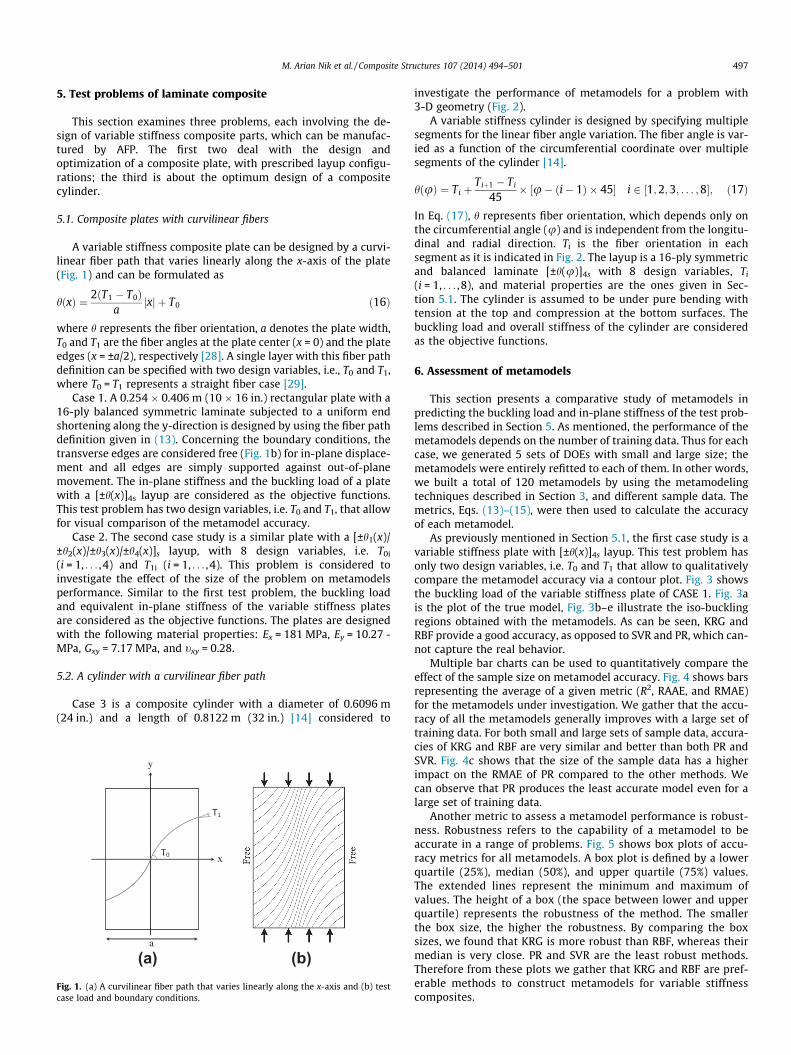
A variable stiffness composite plate can be designed by a curvi-linear fiber path that varies linearly along the x-axis of the plate(Fig. 1) and can be formulated as

hðxÞ ¼ 2ðT1 � T0Þa

jxj þ T0 ð16Þ

where h represents the fiber orientation, a denotes the plate width,T0 and T1 are the fiber angles at the plate center (x = 0) and the plateedges (x = ±a/2), respectively [28]. A single layer with this fiber pathdefinition can be specified with two design variables, i.e., T0 and T1,where T0 = T1 represents a straight fiber case [29].

Case 1. A 0.254 0.406 m (10 16 in.) rectangular plate with a16-ply balanced symmetric laminate subjected to a uniform endshortening along the y-direction is designed by using the fiber pathdefinition given in (13). Concerning the boundary conditions, thetransverse edges are considered free (Fig. 1b) for in-plane displace-ment and all edges are simply supported against out-of-planemovement. The in-plane stiffness and the buckling load of a platewith a [±h(x)]4s layup are considered as the objective functions.This test problem has two design variables, i.e. T0 and T1, that allowfor visual comparison of the metamodel accuracy.

Case 2. The second case study is a similar plate with a [±h1(x)/±h2(x)/±h3(x)/±h4(x)]s layup, with 8 design variables, i.e. T0i

(i = 1, . . . ,4) and T1i (i = 1, . . . ,4). This problem is considered toinvestigate the effect of the size of the problem on metamodelsperformance. Similar to the first test problem, the buckling loadand equivalent in-plane stiffness of the variable stiffness platesare considered as the objective functions. The plates are designedwith the following material properties: Ex = 181 MPa, Ey = 10.27 -MPa, Gxy = 7.17 MPa, and txy = 0.28.

5.2. A cylinder with a curvilinear fiber path

Case 3 is a composite cylinder with a diameter of 0.6096 m(24 in.) and a length of 0.8122 m (32 in.) [14] considered to

(b)(a)

y

Fig. 1. (a) A curvilinear fiber path that varies linearly along the x-axis and (b) testcase load and boundary conditions.

investigate the performance of metamodels for a problem with3-D geometry (Fig. 2).

A variable stiffness cylinder is designed by specifying multiplesegments for the linear fiber angle variation. The fiber angle is var-ied as a function of the circumferential coordinate over multiplesegments of the cylinder [14].

hðuÞ ¼ Ti þTiþ1 � Ti

45 ½u� ði� 1Þ 45� i 2 ½1;2;3; . . . ;8�; ð17Þ

In Eq. (17), h represents fiber orientation, which depends only onthe circumferential angle (u) and is independent from the longitu-dinal and radial direction. Ti is the fiber orientation in eachsegment as it is indicated in Fig. 2. The layup is a 16-ply symmetricand balanced laminate [±h(u)]4s with 8 design variables, Ti

(i = 1, . . . , 8), and material properties are the ones given in Sec-tion 5.1. The cylinder is assumed to be under pure bending withtension at the top and compression at the bottom surfaces. Thebuckling load and overall stiffness of the cylinder are consideredas the objective functions.

6. Assessment of metamodels

This section presents a comparative study of metamodels inpredicting the buckling load and in-plane stiffness of the test prob-lems described in Section 5. As mentioned, the performance of themetamodels depends on the number of training data. Thus for eachcase, we generated 5 sets of DOEs with small and large size; themetamodels were entirely refitted to each of them. In other words,we built a total of 120 metamodels by using the metamodelingtechniques described in Section 3, and different sample data. Themetrics, Eqs. (13)–(15), were then used to calculate the accuracyof each metamodel.

As previously mentioned in Section 5.1, the first case study is avariable stiffness plate with [±h(x)]4s layup. This test problem hasonly two design variables, i.e. T0 and T1 that allow to qualitativelycompare the metamodel accuracy via a contour plot. Fig. 3 showsthe buckling load of the variable stiffness plate of CASE 1. Fig. 3ais the plot of the true model, Fig. 3b–e illustrate the iso-bucklingregions obtained with the metamodels. As can be seen, KRG andRBF provide a good accuracy, as opposed to SVR and PR, which can-not capture the real behavior.

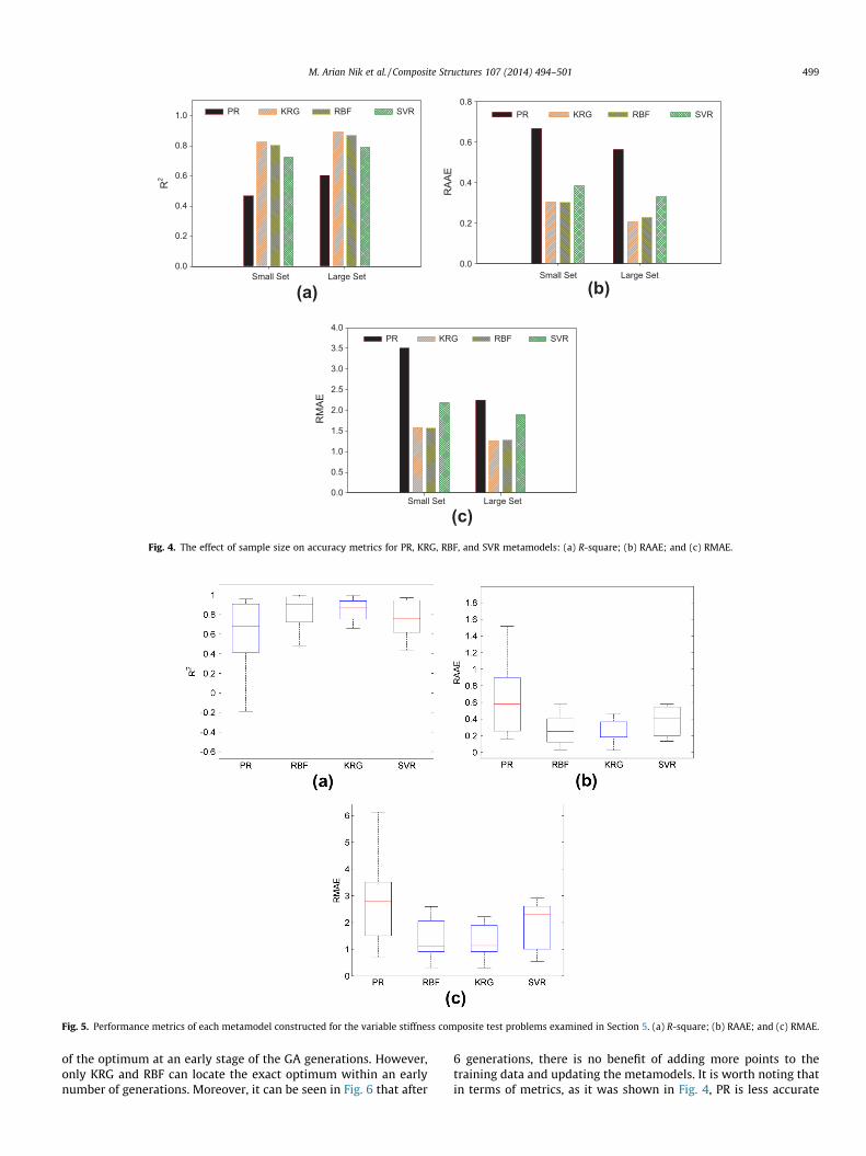
Multiple bar charts can be used to quantitatively compare theeffect of the sample size on metamodel accuracy. Fig. 4 shows barsrepresenting the average of a given metric (R2, RAAE, and RMAE)for the metamodels under investigation. We gather that the accu-racy of all the metamodels generally improves with a large set oftraining data. For both small and large sets of sample data, accura-cies of KRG and RBF are very similar and better than both PR andSVR. Fig. 4c shows that the size of the sample data has a higherimpact on the RMAE of PR compared to the other methods. Wecan observe that PR produces the least accurate model even for alarge set of training data.

Another metric to assess a metamodel performance is robust-ness. Robustness refers to the capability of a metamodel to beaccurate in a range of problems. Fig. 5 shows box plots of accu-racy metrics for all metamodels. A box plot is defined by a lowerquartile (25%), median (50%), and upper quartile (75%) values.The extended lines represent the minimum and maximum ofvalues. The height of a box (the space between lower and upperquartile) represents the robustness of the method. The smallerthe box size, the higher the robustness. By comparing the boxsizes, we found that KRG is more robust than RBF, whereas theirmedian is very close. PR and SVR are the least robust methods.Therefore from these plots we gather that KRG and RBF are pref-erable methods to construct metamodels for variable stiffnesscomposites.

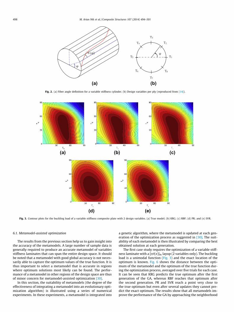
(a) (b)Fig. 2. (a) Fiber angle definition for a variable stiffness cylinder. (b) Design variables per ply (reproduced from [14]).

Fig. 3. Contour plots for the buckling load of a variable stiffness composite plate with 2 design variables. (a) True model; (b) KRG; (c) RBF; (d) PR; and (e) SVR.

498 M. Arian Nik et al. / Composite Structures 107 (2014) 494–501

6.1. Metamodel-assisted optimization

The results from the previous section help us to gain insight intothe accuracy of the metamodels. A large number of sample data isgenerally required to produce an accurate metamodel of variablesstiffness laminates that can span the entire design space. It shouldbe noted that a metamodel with good global accuracy is not neces-sarily able to capture the optimum values of the true function. It isthus important to select a metamodel that is accurate in regionswhere optimum solutions most likely can be found. The perfor-mance of a metamodel in other regions of the design space are thusof minor concern for metamodel-assisted optimization [30].

In this section, the suitability of metamodels (the degree of theeffectiveness of integrating a metamodel into an evolutionary opti-mization algorithm) is illustrated using a series of numericalexperiments. In these experiments, a metamodel is integrated into

a genetic algorithm, where the metamodel is updated at each gen-eration of the optimization process as suggested in [30]. The suit-ability of each metamodel is then illustrated by comparing the bestobtained solution at each generation.

The first case study requires the optimization of a variable stiff-ness laminate with a [±h(x)]4s layup (2 variables only). The bucklingload is a unimodal function (Fig. 3) and the exact location of theoptimum is known. Fig. 6 shows the distance between the opti-mum of the metamodel and the optimum of the true function dur-ing the optimization process, averaged over five trials for each case.It can be seen that KRG predicts the true optimum after the firstgeneration of the GA, whereas RBF reaches that optimum afterthe second generation. PR and SVR reach a point very close tothe true optimum but even after several updates they cannot pre-dict the exact optimum. The results show that all metamodels im-prove the performance of the GA by approaching the neighborhood

(a) (b)

(c)

Small Set Large Set

R2

0.0

0.2

0.4

0.6

0.8

1.0 PR KRG RBF SVR

Small Set Large Set

RAA

E

0.0

0.2

0.4

0.6

0.8PR KRG RBF SVR

Small Set Large Set

RM

AE

0.0

0.5

1.0

1.5

2.0

2.5

3.0

3.5

4.0PR KRG RBF SVR

Fig. 4. The effect of sample size on accuracy metrics for PR, KRG, RBF, and SVR metamodels: (a) R-square; (b) RAAE; and (c) RMAE.

Fig. 5. Performance metrics of each metamodel constructed for the variable stiffness composite test problems examined in Section 5. (a) R-square; (b) RAAE; and (c) RMAE.

M. Arian Nik et al. / Composite Structures 107 (2014) 494–501 499

of the optimum at an early stage of the GA generations. However,only KRG and RBF can locate the exact optimum within an earlynumber of generations. Moreover, it can be seen in Fig. 6 that after

6 generations, there is no benefit of adding more points to thetraining data and updating the metamodels. It is worth noting thatin terms of metrics, as it was shown in Fig. 4, PR is less accurate

Fig. 7. Performance of the metamodels – for the optimization of variable stiffnesslaminates.

500 M. Arian Nik et al. / Composite Structures 107 (2014) 494–501

than SVR; however, it has a better performance when integratedinto the GA. Therefore, a poor metamodel in terms of accuracymetrics does not necessarily have a poor performance when inte-grated into an optimization algorithm.

For the remaining case studies, the optimum design is notknown. Thus to compare the performance of the metamodel-as-sisted optimization algorithms, we use the following relativeimprovement

I ¼ yIBS � yMAO

yIBSð18Þ

where yIBS is the initial best solution and yMAO is the optimum solu-tion found at each generation by the metamodel-assisted optimiza-tion algorithm, and I is the actual improvement over the initial bestsolution. The actual improvement shows how well a metamodel-assisted optimization performs. When there is no improvement inthe solution I = 0; on the other hand, I > 0 represents an improve-ment in the solution. A larger I means a higher improvement inthe solution [31]. The results of the optimization averaged over fivetrials for each case are shown in Fig. 7.

Similar to the previous case, all metamodels have the effect ofenhancing the performance of the optimization process by improv-ing the accuracy of the solution at low number of generations. Forexample, the final best solution found by GA is obtained by allmetamodel-assisted GA after 3 generations only. In other words,for the case studies shown here, the use of the metamodels de-creases of one third the number of generations required by the ge-netic algorithm. The difference between metamodel-assistedalgorithms is significant at early generations and decreases duringthe optimization process. This might be explained by examiningthe evolution of the accuracy during the generations; all modelscan locate the neighborhood of the optimum solution after 5–6generations. Hence, further iteration cannot significantly increasetheir accuracy. In general, RBF followed by KRG outperforms othermethods. In contrast to the previous case, early in the optimizationprocess SVR performs better than PR, yet its superiority over PRdiminishes as the optimization proceeds.

7. Conclusions

This work has compared the performance of alternative meta-modeling methods using multiple criteria for the design optimiza-tion of variable stiffness composite laminates. The metamodelsperformance has been assessed in three case studies. Their accu-racy and robustness in constructing an approximation of the buck-ling load and in-plane stiffness have been measured. The suitabilityof each metamodel for integration into an optimization framework

Fig. 6. Metamodel performance as a function of the number of iterations.Maximization of the buckling load for a [±h(x)]4s composite laminate.

has also been studied. KRG and RBF had the highest accuracy. Interms of robustness, both KRG and RBF provided the best results,where KRG has been slightly better than RBF. In terms of suitabil-ity, KRG has shown the best performance for problems with lownumber of design variables, whereas RBF has been the most appro-priate method for a high number of variables. It is found that theuse of an appropriate metamodel in a metamodel-assisted geneticalgorithm decreases the number of iterations to one-third com-pared to a genetic algorithm.

In this study, the size of the sample data has been consideredfixed. Further investigation is needed to determine the minimumnumber of sample data required to reach a certain level of accuracyfor a given metamodel. In addition, further work is needed toinvestigate the role of kernel and basis functions respectively forKRG and RBF metamodels.

References

[1] Blom A, Setoodeh S, Hol J, Gürdal Z. Design of variable-stiffness conical shellsfor maximum fundamental eigenfrequency. Comput Struct 2008;86:870–8.

[2] Arian Nik M, Fayazbakhsh K, Pasini D, Lessard L. Surrogate-based multi-objective optimization of a composite laminate with curvilinear fibers. ComposStruct 2012;94:2306–23.

[3] Wang GG, Shan S. Review of metamodeling techniques in support ofengineering design optimization. J Mech Des 2007;129:370–80.

[4] Forrester A, Keane A. Recent advances in surrogate-based optimization. ProgAerosp Sci 2009;45:50–79.

[5] Irisarri FX, Laurin F, Leroy FH, Maire JF. Computational strategy formultiobjective optimization of composite stiffened panels. Compos Struct2011;93:1158–67.

[6] Rikards R, Abramovich H, Kalnins K, Auzins J. Surrogate modeling in designoptimization of stiffened composite shells. Compos Struct 2006;73:244–51.

[7] Bisagni C, Lanzi L. Post-buckling optimisation of composite stiffened panelsusing neural networks. Compos Struct 2002;58:237–47.

[8] Liu B, Haftka RT, Akgün MA. Two-level composite wing structural optimizationusing response surfaces. Struct Multidiscipl Optim 2000;20:87–96.

[9] Lee Y-J, Lin C-C. Regression of the response surface of laminated compositestructures. Compos Struct 2003;62:91–105.

[10] Lin C-C, Lee Y-J. Stacking sequence optimization of laminated compositestructures using genetic algorithm with local improvement. Compos Struct2004;63:339–45.

[11] Kalnins K, Rikards R, Auzins J, Bisagni C, Abramovich H, Degenhardt R.Metamodeling methodology for postbuckling simulation of damagedcomposite stiffened structures with physical validation. Int J Struct Stab Dyn2010;10:705–16.

[12] Lanzi L, Giavotto V. Post-buckling optimization of composite stiffened panels:computations and experiments. Compos Struct 2006;73:208–20.

[13] Vandervelde T, Milani AS. Layout optimization of a multi-zoned, multi-layeredcomposite wing under free vibration. In: Proceedings of SPIE, the internationalsociety for optical engineering San Diego, CA, USA; 2009.

[14] Blom AW, Stickler PB, Gürdal Z. Optimization of a composite cylinder underbending by tailoring stiffness properties in circumferential direction. ComposB Eng 2010;41:157–65.

[15] Fayazbakhsh K, Arian Nik M, Pasini D, Lessard L. Defect layer method tocapture effect of gaps and overlaps in variable stiffness laminates made byautomated fiber placement. Compos Struct 2013;97:245–51.

M. Arian Nik et al. / Composite Structures 107 (2014) 494–501 501

[16] Viana FAC, Gogu C, Haftka RT. Making the most out of surrogate models: tricksof the trade. In: ASME conference proceedings; 2010. p. 587–98.

[17] Sacks J, Welch WJ, Mitchell TJ, Wynn HP. Design and analysis of computerexperiments. Stat Sci 1989;4:409–23.

[18] Jin R, Chen W, Simpson TW. Comparative studies of metamodelling techniquesunder multiple modelling criteria. Struct Multidiscip Optim 2001;23:1–13.

[19] Myers RH, Montgomery DC. Response surface methodology: process andproduct optimization using designed experiments. J. Wiley; 2002.

[20] Barton RR. Metamodels for simulation input-output relations. In: Proceedingsof the 24th conference on winter simulation. Arlington, Virginia, USA: ACM;1992. p. 289–99.

[21] Dyn N, Levin D, Rippa S. Numerical procedures for surface fitting of scattereddata by radial functions. SIAM J Sci Stat Comput 1986;7:639–59.

[22] Vapnik VN. Statistical learning theory. Wiley; 1998.[23] Cherkassky V, Ma Y. Practical selection of SVM parameters and noise

estimation for SVM regression. Neural Netw 2004;17:113–26.[24] Gunn SR. Support vector machines for classification and regression. Technical

report, image speech and intelligent systems research group, University ofSouthampton; 1997.

[25] Picard RR, Cook RD. Cross-validation of regression models. J Am Stat Assoc1984:575–83.

[26] Varma S, Simon R. Bias in error estimation when using cross-validation formodel selection. BMC Bioinform 2006;7:91.

[27] Lin Y. An efficient robust concept exploration method and sequentialexploratory experimental design. Atlanta (GA): Georgia Institute ofTechnology; 2004.

[28] Gürdal Z, Olmedo R. In-plane response of laminates with spatially varying fiberorientations: variable stiffness concept. AIAA J 1993;31:751–8.

[29] Gürdal Z, Tatting BF, Wu CK. Variable stiffness composite panels: effects ofstiffness variation on the in-plane and buckling response. Compos A Appl SciManuf 2008;39:911–22.

[30] Ong YS, Nair PB, Keane AJ. Evolutionary optimization of computationallyexpensive problems via surrogate modeling. AIAA J 2003;41:687–96.

[31] Viana F, Haftka R. Surrogate-based optimization with parallel simulationsusing the probability of improvement. In: 13th AIAA/ISSMO multidisciplinaryanalysis optimization conference. Fort Worth (Texas, USA): AIAA; 2010.

[32] Arian Nik M, Fayazbakhsh K, Pasini D, Lessard L. Optimization of variablestiffness composites with embedded defects induced by Automated FiberPlacement. Composite Structures 2014;107:160–6.