2nd

International Conference on Mechanical, Automotive and Aerospace Engineering (ICMAAE 2013) 2-4 July 2013, Kuala Lumpur

A CFD Study of NACA 63415 with deployment of

leading edge and trailing edge surface

W.Z. Wan Omar1,2,a

, M.M.A. Rahim1,b

, T. M. Mat Lazim1,3,c

1Department of Aeronatical, Automotive and Off-shore Engineering, University Teknologi Malaysia, Johor Bahru

Malaysia 2Centre for Electrical Engineering Systems, Energy Reserach Alliance, University Teknologi Malaysia, Johor Bahru

Malaysia 3Transport Research Alliance, Universiti Teknologi Malaysia, Johor Bahru, Malaysia.

awanzaidi@fkm.utm.my,

bmmultazaam2@gmail.com,

ctholudin@fkm.utm.my

ABSTRACT

Deployment of leading edge and trailing edge of airfoils are

methods to improve the aerodynamic characteristics of aerofoils,

and are also used for control purposes. The ability to successfully

obtain specific aerodynamic characteristic is highly dependent on

modifying the aerofoils by combinations of the deployment of

leading and/or trailing edges. Obtaining these characteristics

from wind tunnel tests would involve very high costs. The task is

expected to become simpler with the advancement in computing

power and the Computational Fluid Dynamics (CFD). However

application of CFD needs the right knowledge and expertise. In

the validation phase of this work the initial CFD results for

NACA 63415 without control deflections were compared with

previous published simulations on other platforms and

experimental results. Further CFD studies were then conducted

for 20% chord LE and TE of the NACA 63415 aerofoil deployed

at various angles. The effects of the deployment of leading and

trailing edges to the flow around NACA 63415 aerofoil were also

studied. Results of the aerofoil lift, drag and pitching moment

were presented for a range of angles of attack, and a range of

control surface deflection angles. Another advantage of CFD is its

ability to show the flow behaviour at a particular point of interest

in the flow field. These details might help in understanding and

improving the flow around the aerofoil. The results show that the

maximum lift improved by 14% and the drag reduced by 17%

with a combination of the deployment of the control edges. The

pitching moment coefficient had no significant change.

Keywords- CFD; Aerofoil; control surface; streamline; stall;

turbulence

1. INTRODUCTION

Recent years have seen a significant growth in the size and

investment cost of wind tunnel testing. A good aerodynamic

characteristic is desired in industry to enhance their

performance. However wind tunnel testing is too expensive.

Computational fluid dynamic comes as solution in order to

evaluate the aerodynamic performance. NACA 63415 are

commonly used in wind turbines that suffers multitude of

angles of attack. To enhance the performance the wind

turbines, a good understanding of the aerodynamic

characteristic of the aerofoil are needed including the

performance at or near stall conditions. Mild stall behaviour of

the aerofoil at stall is desired so as to avoid abrupt or violent

unloading of the wind turbine blades after stall. This aerofoil

is also used in aircrafts for its docile stall[1].

This report describes a two-dimensional CFD study done

on NACA 63415 aerofoil with deployment of leading and

trailing edges, from low angles of attack to those past stall.

Specific flow characteristics are presented to understand the

stall mechanism.

The modeling of the problem in CFD is based on co-

ordinates of the aerofoil obtained from UIUC Airfoil

Coordinates Database [2]. The mesh were generated with

ANSYSY 14 workbench, and the CFD calculations were done

in 2D with k-ω SST (shear stress transport) turbulence model

as is recommended in other studiesof flow around aerofoils[3].

The initial validation of the model was done using a NACA

0012 aerofoil whose results from experiments and other CFD

studies are readily available[3].

Figure 1 The NACA 63415 aerofoil[2, 4]

The validated method was then used in this study of the

NACA 63415aerofoil, in clean conditions and with LE and TE

control surfaces deployed. This paper reports the early results

of the study at angles of attack (AOA) from -6O to 21

O which

covers the flying conditions and the early stall conditions, with

and without control surface deployments.

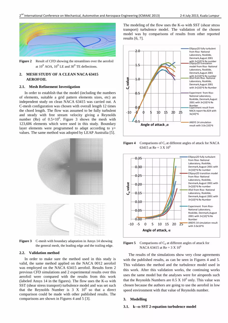
Another advantage of the CFD study is the ability to

visualize and scrutinize the flow details in the domain studied.

In understanding the stall mechanics, specific points on the

aerofoil where the flow starts to separate is of very high

interests. The flow separation mechanics can be studied in

detail and if any modification is carried out, its effects can be

studied with less trouble compared to physical wind tunnel

tests. This particular part of the study is not reported in this

paper, as it would only come in the next phase of this research

work, but an example of a single condition of 10ο AOA,

10οLE and 30

οTE deflections is shown in Figure 2 to

emphasize the importance of this function in CFD method.

Here the flow separation can clearly be seen at the junction of

the main aerofoil to TE intersection.

2nd

International Conference on Mechanical, Automotive and Aerospace Engineering (ICMAAE 2013) 2-4 July 2013, Kuala Lumpur

Figure 2 Result of CFD showing the streamlines over the aerofoil

at 10ο AOA, 10

ο LE and 30

ο TE deflections.

2. MESH STUDY OF A CLEAN NACA 63415

AEROFOIL

2.1. Mesh Refinement Investigation

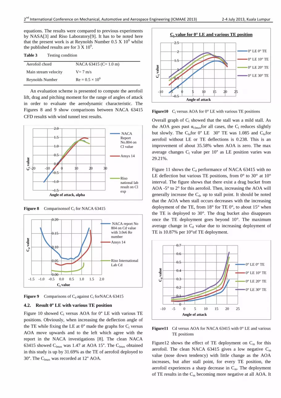
In order to establish that the model (including the numbers

of elements, suitable a grid pattern elements sizes, etc) an

independent study on clean NACA 63415 was carried out. A

C-mesh configuration was chosen with overall length 12 times

the chord length. The flow was assumed to be fully turbulent

and steady with free stream velocity giving a Reynolds

number (Re) of 0.5×106. Figure 3 shows the mesh with

123,606 elements which were used in this study. Boundary

layer elements were programmed to adapt according to y+

values. The same method was adopted by LEAP Australia [5].

Figure 3 C-mesh with boundary adaptation in Ansys 14 showing

the general mesh, the leading edge and the trailing edge.

2.2. Validation method

In order to make sure the method used in this study is

valid, the same method applied on the NACA 0012 aerofoil

was employed on the NACA 63415 aerofoil. Results form 2

previous CFD simulations and 2 experimental results over this

aerofoil were compared with the results from this work

(labeled Ansys 14 in the figures). The flow uses the K-ω with

SST (shear stress transport) turbulence model and was set such

that the Reynolds Number is 3 X 106

so that a direct

comparison could be made with other published results. The

comparisons are shown in Figures 4 and 5 [3].

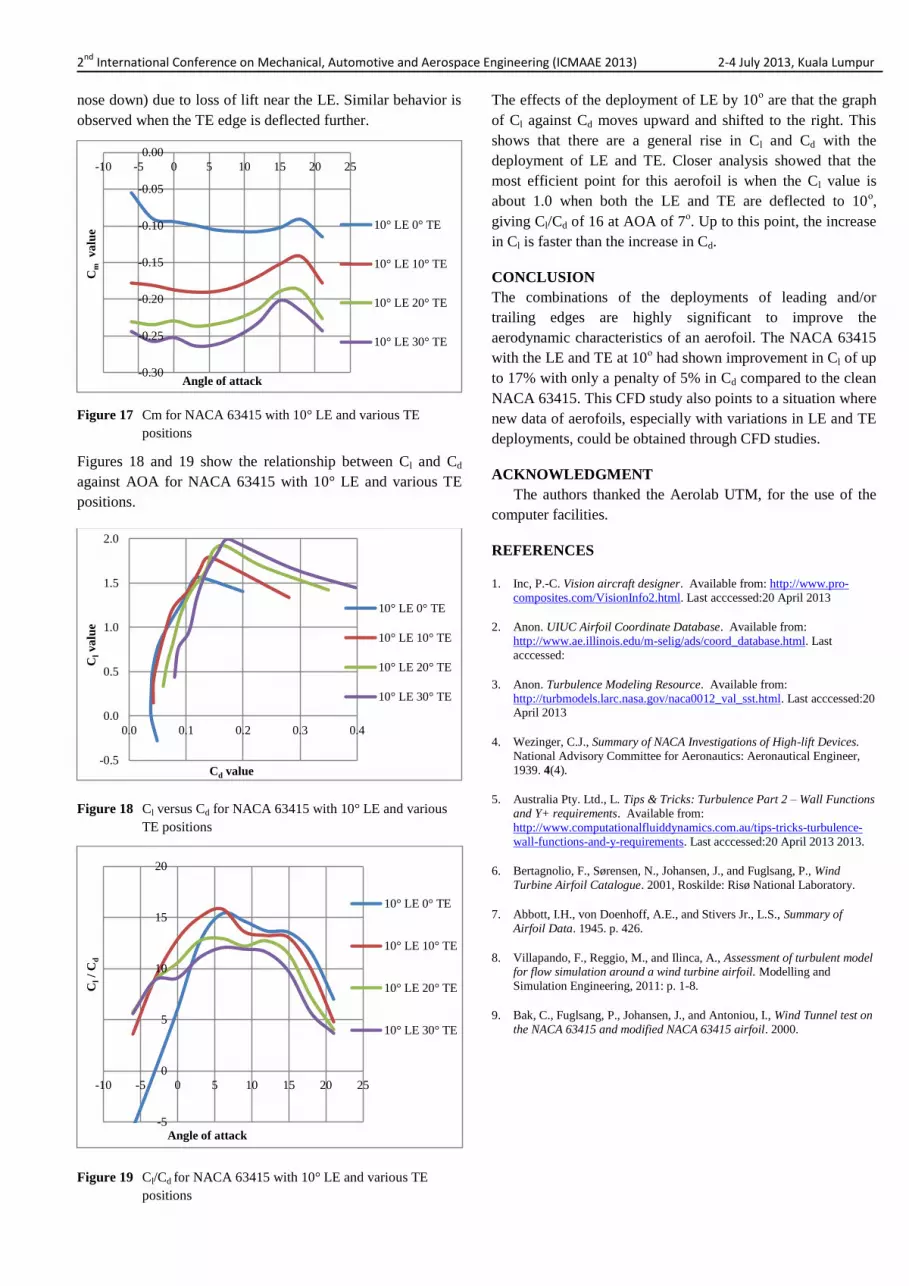
The modeling of the flow uses the K-ω with SST (shear stress

transport) turbulence model. The validation of the chosen

model was by comparisons of results from other reported

results [6, 7].

Figure 4 Comparisons of Cl at different angles of attack for NACA

63415 at Re = 3 X 106

Figure 5 Comparisons of Cd at different angles of attack for

NACA 63415 at Re = 3 X 106

The results of the simulations show very close agreements

with the published results, as can be seen in Figures 4 and 5.

This validates the method and the turbulence model used in

this work. After this validation works, the continuing works

uses the same model but the analyses were for airspeeds such

that the Reynolds Numbers are 0.5 X 106 only. This value was

chosen because the authors are going to use the aerofoil in low

speed environment with that value of Reynolds number.

3. Modelling

3.1. k--ω SST 2-equation turbulence model

-0.5

0.0

0.5

1.0

1.5

2.0

-10 -5 0 5 10 15 20 25

Cl v

alu

e

Angle of attack ,α

Ellipsys2D fully turbulentfrom Riso- NationalLaboratory, Roskilde,Denmark,August 2001with 3×[10]^6 Re numberEllipsys2D transiationmodel from Riso- NationalLaboratory, Roskilde,Denmark,August 2001with 3×[10]^6 Re numberXfoil from Riso- NationalLaboratory, Roskilde,Denmark,August 2001with 3×[10]^6 Re Number

Experiment from Riso-National Laboratory,Roskilde, Denmark,August2001 with 3×[10]^6 ReNumberExperiment result fromNACA report No.824 with3x[10]^6

ANSYS 14 simulationresult with 3.0x [10]^6

0.00

0.05

0.10

0.15

0.20

0.25

0.30

0.35

-10 -5 0 5 10 15 20 25

Cd v

alu

e

Angle of attack, α

Ellipsys2D fully turbulantfrom Riso- NationalLaboratory, Roskilde,Denmark,August 2001 with3×[10]^6 Re number

Ellipsys2D transition modelfrom Riso- NationalLaboratory, Roskilde,Denmark,August 2001 with3×[10]^6 Re number

Xfoil from Riso- NationalLaboratory, Roskilde,Denmark,August 2001 with3×[10]^6 Re Number

Experiment from Riso-National Laboratory,Roskilde, Denmark,August2001 with 3×[10]^6 ReNumber

ANSYS 14 simulation resultwith 3.0x10^6

2nd

International Conference on Mechanical, Automotive and Aerospace Engineering (ICMAAE 2013) 2-4 July 2013, Kuala Lumpur

The k-ω SST 2-equation turbulence model is able to work

with either Wall Functions or fully resolve the boundary layer,

so the same y+ conditions apply. Therefore, the acceptable y+

value are 30 to 300 [5], or a y+ of 1 if the flow has adverse

pressure gradients or separation regions that need to be

properly resolved. The use of scalable wall functions will

automatically activate the local usage of the log law in regions

where the y+ is sufficiently small to fully resolve the boundary

layer, in conjunction with the standard wall function approach

in any regions where the y+ is coarser.

K-ω SST model is reputed to be more accurate than k-€ in

near wall layer. It has been successful for flow with moderate

adverse pressure gradient [5], it have ω equation which very

sensitive to the value of ω in the free stream. The SST corrects

this problem by solving the standard k-ω in the far field and

the standard k-ω near the wall. To improve its performance for

adverse pressure flow, the SST considers the effects of the

transport of the turbulent shear stresses in the calculations of

the turbulent viscosity and turbulent Prandtl number[5].

Thus a good approximation of flow in this study was

obtained using k-ω SST. It gives us better result of Cd

prediction.

The accuracy computational turbulent viscosity near skin is

very important in order to study flow around airfoil with low

Reynolds number. The k-ω SST turbulent model was chosen

as turbulence model solver in this study. Figure 6 shows that

k-ω SST gives better resolution of eddies at the trailing edge.

It uses the multiple circulation graphic to visualize the eddy

flow[8].

Figure6 streamlines at the trailing edge using k-ω SST[8].

3.2. Element type

In this study, the NACA 63415 was modeled in

SolidWorks. The variable parameter of LE and TE edge

deployment was setup according to the desired angles in

SolidWorks. The summary of the angles of deployment can be

seen in Table 2.

The mesh selection is highly dependent on geometry of the

subject. Since the aerofoil with the control surface deflections

does not have complex geometry, the structured mesh was

chosen. C- Mesh configuration with boundary adaptation was

used in this study as shown in Figure3. The far-field size was

setup 12 times chord length. Structured elements used in this

study were the quadrilateral element type. The mesh was

controlled based on bias factor and number of divisions of the

elements themselves. The frontal area of the c-mesh

configuration was setup with 0 bias factors and 100 number of

division of elements. The rest of edge was setup with 150 bias

factor and 200 number of division elements. Table

1summarises the element types used in this study.

Table 1 Summary of mesh characteristics

Far field configuration C- mesh

Number of quadrants 4

Front bias factor 0

Quadrant bias factor 150

Front number of division 100

Quadrant number of division 200

Number of element 123606

Number of node 124811

Range of Y+ 1-12

3.3. Case studies

The flow over the aerofoil were analysed and the resulting

Cl and Cd were noted for various control deflections. The

leading edge deflections studied were from 0° to 15°

downward with increments of 5°, while the deflections of the

trailing edge were from 0° to 30° with increments of 10°. The

total cases are 16. At each control deflection case, the

simulations were run at angles of attack from -6° to 21° with

increments of 3°.All cases are summarised in Table 2 and the

diagram of the aerofoil in different configurations is shown in

Figure 7.

Table 2 Summary of cases studied

Sim no. Leading edge deflection

(Degree)

Trailing edge deflection

(Degree)

1 0 0

2 0 10

3 0 20

4 0 30

5 5 0

6 5 10

7 5 20

8 5 30

9 10 0

10 10 10

11 10 20

12 10 30

13 15 0

14 15 10

15 15 20

16 15 30

Figure 7 The Aerofoil with the defelected positions of the LE and

TE control surfaces

4. RESULT

4.1. Test condition and comparison with previous result

The conditions for the simulations as reported in this paper

are summarized in Table 3. The calculations were all done

with steady 7 m/s flow with turbulence model k-ω SST 2

2nd

International Conference on Mechanical, Automotive and Aerospace Engineering (ICMAAE 2013) 2-4 July 2013, Kuala Lumpur equations. The results were compared to previous experiments

by NASA[3] and Riso Laboratory[9]. It has to be noted here

that the present work is at Reynolds Number 0.5 X 106 whilst

the published results are for 3 X 106.

Table 3 Testing condition

Aerofoil chord NACA 63415 (C= 1.0 m)

Main stream velocity V= 7 m/s

Reynolds Number Re = 0.5 × 106

An evaluation scheme is presented to compute the aerofoil

lift, drag and pitching moment for the range of angles of attack

in order to evaluate the aerodynamic characteristic. The

Figures 8 and 9 show comparisons between NACA 63415

CFD results with wind tunnel test results.

Figure 8 Comparisonsof Cl for NACA 63415

Figure 9 Comparisons of Cd against Cl forNACA 63415

4.2. Result 0° LE with various TE position

Figure 10 showed Cl versus AOA for 0° LE with various TE

positions. Obviously, when increasing the deflection angle of

the TE while fixing the LE at 0° made the graphs for Cl versus

AOA move upwards and to the left which agree with the

report in the NACA investigations [8]. The clean NACA

63415 showed Clmax was 1.47 at AOA 15°. The Clmax obtained

in this study is up by 31.69% as the TE of aerofoil deployed to

30°. The Clmax was recorded at 12° AOA.

Figure10 Cl versus AOA for 0° LE with various TE positions

Overall graph of Cl showed that the stall was a mild stall. As

the AOA goes past αclmaxfor all cases, the Cl reduces slightly

but slowly. The Clofor 0° LE 30° TE was 1.085 and Clofor

aerofoil without LE or TE deflections is 0.238. This is an

improvement of about 35.58% when AOA is zero. The max

average changes Cl value per 10° as LE position varies was

29.21%.

Figure 11 shows the Cd performance of NACA 63415 with no

LE deflection but various TE positions, from 0° to 30° at 10°

interval. The figure shows that there exist a drag bucket from

AOA -5° to 2° for this aerofoil. Then, increasing the AOA will

generally increase the Cd, up to stall point. It should be noted

that the AOA when stall occurs decreases with the increasing

deployment of the TE, from 18° for TE 0°, to about 15° when

the TE is deployed to 30°. The drag bucket also disappears

once the TE deployment goes beyond 10°. The maximum

average change in Cd value due to increasing deployment of

TE is 10.87% per 10°of TE deployment.

Figure11 Cd versus AOA for NACA 63415 with 0° LE and various

TE positions

Figure12 shows the effect of TE deployment on Cm for this

aerofoil. The clean NACA 63415 gives a low negative Cm

value (nose down tendency) with little change as the AOA

increases, but after stall point, for every TE position, the

aerofoil experiences a sharp decrease in Cm. The deployment

of TE results in the Cm becoming more negative at all AOA. It

-1.5

-1.0

-0.5

0.0

0.5

1.0

1.5

2.0

-20 -10 0 10 20 30Cl v

alu

e

Angle of attack, alpha

NACA

ReportNo.804 on

Cl value

Ansys 14

Riso

national labresult on Cl

exp

0.00

0.05

0.10

0.15

0.20

-1.5 -1.0 -0.5 0.0 0.5 1.0 1.5 2.0

Cd v

alu

e

Cl value

NACA report No

804 on Cd valuewith 3.0e6 Re

number

Ansys 14

Riso International

Lab Cd

-0.5

0

0.5

1

1.5

2

2.5

-10 -5 0 5 10 15 20 25

Cl v

alu

e

Angle of attack

Cl value for 0° LE and various TE position

0° LE 0° TE

0° LE 10° TE

0° LE 20° TE

0° LE 30° TE

0

0.1

0.2

0.3

0.4

0.5

0.6

0.7

-10 -5 0 5 10 15 20 25

Cd v

alu

e

Angle of attack

0° LE 0° TE

0° LE 10° TE

0° LE 20° TE

0° LE 30° TE

2nd

International Conference on Mechanical, Automotive and Aerospace Engineering (ICMAAE 2013) 2-4 July 2013, Kuala Lumpur should also be noted that when the TE is deployed, Cm

increases when the AOA increases from 0° to about 8°.

Figure12 Cm versus AOA for NACA 63415 with 0° LE and

various TE positions

Figures13 and 14 show the relationship between Cl, Cd and the

AOA for various TE positions, but without LE being

deployed.Figure9 shows that overall, the Cd increase with the

deployment of the TE, and so is the Cl. But the improvement

stops when the airfoil stalls, which occurs at lower AOA as

the TE is deflected further downwards. Figure 13 shows that

the best Cl/Cd of about 17 is obtained with the aerofoil at AOA

of 3° and with the TE deployed to 10°.

Figure13 Cl versus Cd for NACA63415 with 0° LE and various

TE positions

Figure 14 Cl /Cd versus AOA of NACA 63415 with 0° LE and

various TE positions

4.3. Results for 10° LE with various TE positions

Figure 15 shows the Cl against AOA for 10° LE deployment

with various TE positions. The deployment of the LE

generally has the effect of extending the stall point (the Cl

increases until a new stall point is reached) past the point of

stall when the LE is not deployed, which agrees with results

from others [7]. The average increase in stalling angle and Cl

increase are about +2° and 8.2% respectively per 10° of LE

deployment.

Figure 16 explains the effects on Cd when LE was deployed.

The most interesting effect of LE deployment on Cd values is

the improvement of the range of the drag bucket when the TE

is not deployed. The drag bucket for 0° LE 0° TE was from -

5° to 0° AOA, while the drag buckets for 10° LE 0° TE is

from -5° to 6° AOA. The drag bucket is not apparent once the

TE is deployed.

Figure 15 Cl for NACA 63415 with 10° LE and various TE

positions

Figure 16 Cd for NACA 63415 with 10° LE and various TE

positions

Figure 17 shows the variations of Cmfor the aerofoil with 10°

LE deflection and various TE deflections. For TE at 0° the Cm

continuously reduces (tending to nose down) with AOA, until

the stall point where it increases (reduced nose down

tendency) sharply. Then Cm reduces further (continue to tend

-0.4

-0.3

-0.2

-0.1

0

-10 -5 0 5 10 15 20 25

Cm

va

lue

Angle of attack

0° LE 0° TE

0° LE 10° TE

0° LE 20° TE

0° LE 30° TE

-0.5

0.0

0.5

1.0

1.5

2.0

0.0 0.2 0.4 0.6

Cl v

alu

e

Cd value

0° LE 0° TE

0° LE 10° TE

0° LE 20° TE

0° LE 30° TE

-10

-5

0

5

10

15

20

-10 -5 0 5 10 15 20 25

Cl /

Cd

Angle of attack

0° LE 0° TE

0° LE 10° TE

0° LE 20° TE

0° LE 30° TE

-0.5

0.0

0.5

1.0

1.5

2.0

2.5

-10 -5 0 5 10 15 20 25

Cl v

alu

e

Angle of attack

10° LE 0° TE

10° LE 10° TE

10° LE 20° TE

10° LE 30° TE

0.0

0.1

0.2

0.3

0.4

-10 -5 0 5 10 15 20 25

Cd v

alu

e

Angle of attack

10° LE 0° TE

10° LE 10° TE

10° LE 20° TE

10° LE 30° TE

2nd

International Conference on Mechanical, Automotive and Aerospace Engineering (ICMAAE 2013) 2-4 July 2013, Kuala Lumpur nose down) due to loss of lift near the LE. Similar behavior is

observed when the TE edge is deflected further.

Figure 17 Cm for NACA 63415 with 10° LE and various TE

positions

Figures 18 and 19 show the relationship between Cl and Cd

against AOA for NACA 63415 with 10° LE and various TE

positions.

Figure 18 Cl versus Cd for NACA 63415 with 10° LE and various

TE positions

Figure 19 Cl/Cd for NACA 63415 with 10° LE and various TE

positions

The effects of the deployment of LE by 10ο are that the graph

of Cl against Cd moves upward and shifted to the right. This

shows that there are a general rise in Cl and Cd with the

deployment of LE and TE. Closer analysis showed that the

most efficient point for this aerofoil is when the Cl value is

about 1.0 when both the LE and TE are deflected to 10ο,

giving Cl/Cd of 16 at AOA of 7ο. Up to this point, the increase

in Cl is faster than the increase in Cd.

CONCLUSION

The combinations of the deployments of leading and/or

trailing edges are highly significant to improve the

aerodynamic characteristics of an aerofoil. The NACA 63415

with the LE and TE at 10ο had shown improvement in Cl of up

to 17% with only a penalty of 5% in Cd compared to the clean

NACA 63415. This CFD study also points to a situation where

new data of aerofoils, especially with variations in LE and TE

deployments, could be obtained through CFD studies.

ACKNOWLEDGMENT

The authors thanked the Aerolab UTM, for the use of the

computer facilities.

REFERENCES

1. Inc, P.-C. Vision aircraft designer. Available from: http://www.pro-

composites.com/VisionInfo2.html. Last acccessed:20 April 2013

2. Anon. UIUC Airfoil Coordinate Database. Available from:

http://www.ae.illinois.edu/m-selig/ads/coord_database.html. Last

acccessed:

3. Anon. Turbulence Modeling Resource. Available from:

http://turbmodels.larc.nasa.gov/naca0012_val_sst.html. Last acccessed:20 April 2013

4. Wezinger, C.J., Summary of NACA Investigations of High-lift Devices.

National Advisory Committee for Aeronautics: Aeronautical Engineer,

1939. 4(4).

5. Australia Pty. Ltd., L. Tips & Tricks: Turbulence Part 2 – Wall Functions

and Y+ requirements. Available from:

http://www.computationalfluiddynamics.com.au/tips-tricks-turbulence-

wall-functions-and-y-requirements. Last acccessed:20 April 2013 2013.

6. Bertagnolio, F., Sørensen, N., Johansen, J., and Fuglsang, P., Wind

Turbine Airfoil Catalogue. 2001, Roskilde: Risø National Laboratory.

7. Abbott, I.H., von Doenhoff, A.E., and Stivers Jr., L.S., Summary of

Airfoil Data. 1945. p. 426.

8. Villapando, F., Reggio, M., and Ilinca, A., Assessment of turbulent model for flow simulation around a wind turbine airfoil. Modelling and

Simulation Engineering, 2011: p. 1-8.

9. Bak, C., Fuglsang, P., Johansen, J., and Antoniou, I., Wind Tunnel test on

the NACA 63415 and modified NACA 63415 airfoil. 2000.

-0.30

-0.25

-0.20

-0.15

-0.10

-0.05

0.00

-10 -5 0 5 10 15 20 25

Cm

va

lue

Angle of attack

10° LE 0° TE

10° LE 10° TE

10° LE 20° TE

10° LE 30° TE

-0.5

0.0

0.5

1.0

1.5

2.0

0.0 0.1 0.2 0.3 0.4

Cl v

alu

e

Cd value

10° LE 0° TE

10° LE 10° TE

10° LE 20° TE

10° LE 30° TE

-5

0

5

10

15

20

-10 -5 0 5 10 15 20 25

Cl /

Cd

Angle of attack

10° LE 0° TE

10° LE 10° TE

10° LE 20° TE

10° LE 30° TE