Proceedings of the 2000 6

TH IEEE International Workshop on

Cellular Neural Networks and their Applications

(CNNA 2000)

DISTRIBUTION STATEMENT A Approved for Public Release

Distribution Unlimited

Dipartimento Elettrico Elettronico e Sistemistico Universitä degli Studi di Catania

Catania, Italy May 23-25,2000

20010817 074 IEEE

IEEE 00TH8509

REPORT DOCUMENTATION PAGE Form Approved OMB No. 0704-0188

Public reporting burden for this collection of information is estimated to average 1 hour per response, including the time for reviewing instructions, searching existing data sources, gathering and maintaining the data needed, and completing and reviewing the collection of information. Send comments regarding this burden estimate or any other aspect of this collection of information, including suggestions for reducing this burden to WashingtöfTHeädquarters Services, Directorate for Information Operations/?„".d Reports, 1215 Jefferson Davis Highway, Suite 1204, Arlington, VA 22202-4302, and to the Office of Management and Budget, Paperwork Reduction Project (0704-0188), Washington, DC 20503. 1. AGENCY USE ONLY (Leave blank) 2. REPORT DATE

23 May 2000

3. REPORT TYPE AND DATES COVERED

Conference Proceedings

4. TITLE AND SUBTITLE

6th Intl. Workshop on Cellular Neural Networks & Applications

6. AUTHOR(S)

Conference Committee

5. FUNDING NUMBERS

F61775-00-WF055

7. PERFORMING ORGANIZATION NAME(S) AND ADDRESS(ES)

Universita di Catania Viale Andrea Doria 6 Catania 95125 Italy

8. PERFORMING ORGANIZATION REPORT NUMBER

N/A

9. SPONSORING/MONITORING AGENCY NAME(S) AND ADDRESS(ES)

EOARD PSC 802 BOX 14 FPO 09499-0200

10. SPONSORING/MONITORING AGENCY REPORT NUMBER

CSP 00-5055

11. SUPPLEMENTARY NOTES

12a. DISTRIBUTION/AVAILABILITY STATEMENT

Approved for public release; distribution is unlimited.

12b. DISTRIBUTION CODE

A

13. ABSTRACT (Maximum 200 words)

The Final Proceedings for 6th Intl. Workshop on Cellular Neural Networks & Applications, 23 May 2000 - 25 May 2000

This is an interdisciplinary conference. Topics include basic theory of cellular nonlinear spatiotemporal phenomena, physical implementations (VLSI, Optical, Nanotechnology), CNN computers, biologically inspired intelligent robots, and sensor networks for data fusion and real time control.

14. SUBJECT TERMS

EOARD, Computational Mathematics

15. NUMBER OF PAGES

462 16. PRICE CODE

N/A 17. SECURITY CLASSIFICATION

OF REPORT

UNCLASSIFIED

18. SECURITY CLASSIFICATION OF THIS PAGE

UNCLASSIFIED

19, SECURITY CLASSIFICATION OF ABSTRACT

UNCLASSIFIED

20. LIMITATION OF ABSTRACT

UL NSN 7540-01-280-5500 Standard Form 298 (Rev. 2-89)

Prescribed by ANSI Std. 239-18 298-102

Proceedings of the 2000 6TH

IEEE International Workshop on

Cellular Neural Networks and their Applications

(CNNA 2000)

Dipartimento Elettrico Elettronico e Sistemistico Universitä degli Studi di Catania

Catania, Italy May 23-25,2000

IEEE

IEEE00TH8509 ffi W ll-fitf

Copyright and Reprint Permission: Abstracting is permitted with credit to the source. Libraries arc permitted tö photocopy beyond the limit of U.S. copyright law for private use of patrons those articles in this volume that carry a code at the bottom of the first page, provided the per-copy fee indicated in the code is paid through Copyright Clearance Center, 222 Rosewood Drive, Danvers, MA 01923. For other copying, reprint or republication permission, write to IEEE Copyrights Manager, IEEE Operations Center, 445 Hoes Lane, P.O. Box 1331, Piscataway, NJ 08855-1331. All rights reserved. Copyright ©2000 by the Institute of Electrical and Electronics Engineers, Inc.

IEEE Catalog Number O0TH8509 ISBN 0-7803-6344-2 Library of Congress Number 00-01526

CNNA 2000 ßth JEEE international Workshop on

Cellular Neural Networks and their Applications

Catania, 23-25 May 2000, Catania

ACKNOWLEDGEMENT

The Organizing and Scientific Committee wish to thank the following for their contribution to the success of this conference:

• IEEE Circuit and Systems Society

• European Office of Aereospace Research and Development, Air Force Office of Scientific Research, United States Air Force Research Laboratory

• Office of Naval Research Europe

• Universitä degli Studi di Catania

• Regione Siciliana

• Ministero degli Affari Esteri, Direzione Generale per la Promozione e la Cooperazione Culturale, Roma

• ST Microelectronics, Catania

• Yamaha Motor Europe

• Accent

• Azienda Provinciale Turismo, Catania

Foreword

This volume of the Proceedings of the Sixth International Workshop on Cellular Neural Networks and their Applications contains all the contributions to CNNA2000. The Symposium has been organized by the Department of Electrical, Electronic and System Engineering of the Universita degli Studi di Catania and by the Soft Computing Group of ST Microelectronics. The Symposium is co-sponsored by the IEEE Circuits and System Society.

In this volume many excellent contributions regarding the various areas of CNN Technology, including research and development, are included. People from more than 20 countries world-wide will present their latest results concerning theoretical aspects, applications, and hardware implementation. Particular attention has been paid to new trends of research, beyond traditional real-world applications, in an attempt of leading a path for the CNN research of the new millenium.

The University of Catania, one of the oldest of Italy, founded in 1434, is very happy to host the symposium, together with the Administrative council, the Academic Senate, and the Dean of the Engineering Faculty, and warmly greeting the attendees to the symposium. It is a great honour for all of us to have the opportunity to celebrate Prof. Leon O. Chua, conferring him the Laurea ad Honorem, with a ceremony which will be held after the Plenary Session, during the first day of the symposium.

CNN research and applications span a great variety of fields and has raised increasing attention from scientists and engineers coming from different research areas. In particular, Catania has become a relevant pole in CNN research, involving both academic and industrial research teams, as the System and Control Group of the Electric, Electronic and System Department, the Soft Computing Group of ST Microelectronics, and the National Research Council (CNR), which impressively develops applications devoted to the monitoring of Etna volcanic eruptions. In this framework, Cellular Neural Networks are widely treated in an undergraduate course.

A short course in CNN, held by the last year students, will parallel the conference with the aim of presenting the fundamentals of CNN Technology to the younger students. The Organizing Committee of CNNA2000 is glad to host also the Nonlinear Dynamics of Electronic Systems Workshop, NDES2000, joined to CNNA2000 as in Seville, 1996.

The Conference site is located within the University Campus, to promote the fascinating subjects of CNN Technology to students, researchers, and people not yet involved in this field.

We are very grateful to the IEEE Circuits and Systems Society (CAS), the Office of Naval Research Europe (ONR), ST Microelectronics (Catania site), Accent, Yamaha Motors Europe, Universita degli Studi di Catania, Regione Siciliana, Ministero degli Affari Esteri (Roma) who sponsored this Symposium, and to the Scientific Committee.

My special thanks are to the students of the Adaptive Systems course and to the IEEE Student Branch of Catania, who kindly supported the organization of the events.

I cannot conclude this foreword without reminding the continuous encouragement of my students and alumni, who contributed with their works to the growth of the University of Catania as a relevant research pole of the Mediterranean area.

Catania, May, 2000

Luigi Fortuna

Scientific Committee:

L.O. Chua USA V. Cimagalli A.S. Dimitriev

Italy Russia

G. Guzelis M. Hasler

Turkey Switzerland

J. Herault France J.L. Huertas S. Jankowski

Spain Poland

J.A. Nossek J. Pineda de Gyvez V. Porra

Germany USA Finland

A. Rodriguez-Vazquez T. Roska B. Sheu

Spain Hungary USA

M. Tanaka V. Tavsanoglu J. Vandewalle

Japan UK Belgium

Conference Organization:

CNNA2000 Dipartimento Elettrico Elettronico e Sistemistico Facolta di Ingegneria, Universita di Catania, Viale Andrea Doria, 6 - 95125 Catania, Italy fax: +39 095 339535 e-mail: gmarlet@dees.unict.it, lfortuna@dees.unict.it

Organising Committee:

L. Fortuna University of Catania, General Chair P. Arena University of Catania L. Carnimeo Politecnico di Bari M. Gilli Politecnico di Torino L. Occhiplnti STMicroelectronics, Catania G. Palumbo University of Catania F. Sargeni University of Rome 'Tor Vergata"

Co-sponsored by:

IEEE Circuits and Systems Society Universita degli Studi di Catania ACCENT Regione Siciliana Office of Naval Research Europe ST Microelectronics Catania Yamaha Motor Europe Ministero Affari Esteri, Direzione Generale per la Promozione e la Cooperazione Culturale, Roma

TABLE OF CONTENTS

Lectio Magistralis

L.O. Chua "Universal CNN Cells"

Session Theory I

I. Petras, T. Roska i

"Application of Direction Constrained and Bipolar Waves for Pattern Recognition"

P. Szolgay, T. Hidvegi, Z. Szolgay, P. Kozma 9

"A Comparison of the Different CNN Implementations in Solving the Problem of Spatiotemporal Dynamics in Mechanical Systems"

C.Rekeczky,B. Roska, E. Nemeth, F. Werblln 15

"Neuromorphic CNN Models for Spatio-Temporal Effects Measured in the Inner and Outer Retina of Tiger Salamander"

V.Mladenov, H.Hegt 21

"On Waves and Recovering in One-dimensional Autonomous CNNs"

L. Goras, T. Teodorescu, A. Maiorescu 27

"Phase Influence on Mode Competition in Turing Pattern Formation"

V.G.Yakhno ( 33

"Dynamics of Autowave Processes in Neuron-Like Systems and CNN Technology"

Session Applications I

D. Monnin, L. Merlat, A. Köneke, J. Herault 39 "Straightforward Design of Robust Cellular Neural Networks for Image Processing"

I.V. Nuidel, V.G.Yakhno 45

"Modelling of Extraction of Image Fragments in the Forms of Crosses and Rhombuses in the Simulated Receptive Fields"

L. Czüni, T. Sziränyi 51

"Motion Segmentation and Tracking Optimization with Edge Relaxation in the Cellular Nonlinear Network Architecture"

M.Tanaka,Y.Tanji,M.Onishi,T.Nakaguchi 57

"Lossless Image Compression and Recontruction by Cellular Neural Networks"

V. Tavsanoglu, E. Saatci 63

'Teature Extraction for Character Recognition Using Gabor-type Filters Implemented by Cellular Neural Networks"

B.E. Shi "Subthreshold Implementation of a 2D CNN Gabor-type Focal Plane Filter"

Plenary Session

T. Roska "Analogic Computing: System Aspects of Analogic CNN Sensor Computers"

69

73

VII

Demo Session

A. Zarändy, S. Espejo, P. Földesy, L. Kek, G. Linan, C. Rekeczky, A. Rodriguez- Väzquez, T. Roska, I. Szatmari, T. Sziränyi, P. Szolgay "CNN Technology in Action"

M. Balsi "Regularization-Based Continuous-Time Motion Detection by Single-Layer Cellular Neural Networks"

79

Session Poster I

M. Mori, M. Matsuyama, Y. Tanji, M. Tanaka 83 "CNN Image Compression and Reconstruction Based on Non-Orthogonal Wavelet Transform"

N.K. AI-Ani, T. Kacprzak 87

"Time-Varying Cellular Neural Network Based Morphological Image Processing"

M. Brendel, T. Roska 93 "Adaptive Image Sensing and Enhancement Using the Adaptive Cellular Neural Network Universal Machine"

A. Gacsädi, P. Szolgay 99 "An Analogic CNN Algorithm for Following Continuously Moving Objects"

V. Gäl, T. Roska 105

"Collision Prediction via the CNN Universal Machine"

L. Orzo j j j "Optimal CNN Templates for Deconvolution"

A. Zanela, S. Taraglio 117 "A Cellular Neural Network Stereo Vision System for Autonomous Robot Navigation"

A. Loncar, R. Kunz, R. Tetzlaff J23 "SCNN 2000 - Part I: Basic Structure and Features of the Simulation System for Cellular Neural Networks"

R. Kunz, A. Loncar, R. Tetzlaff 129 "SCNN 2000 - Part II: The Simulation Control System"

135

G. Grassi, G. Acciani 141 "Heteroassociative Memories via Globally Asymptotically Stable Discrete-Time Cellular Neural Networks"

C. Amenta, P. Arena, S. Baglio, L. Fortuna, D. Richiusa, M.G. Xibilia, L. Vullo 147 "SC-CNNs for Sensor Data Fusion and Control in Space Distributed Structures"

P. Arena, L. Bertucco, R. Caponetto, L. Fortuna, G. Nunnari, D. Porto 153 "Autowaves in Noninteger Order CNNs"

L. Bertucco, G. Fargione, G. Nunnari, A. Risitano 159 "A Cellular Neural Networks Approach for Non-Destructive Control of Mechanical Parts"

Session Advanced Theory

D. Bälya, B. Roska, E. Nemeth, T. Roska, F. Werblin 165 "A Qualitative Model-Framework for Spatio-temporal Effects in Vertebrate Retinas"

VIII

A. Loncar, R. Tetzlaff 171

"Cellular Neural Networks with Nearly Arbitrary Nonlinear Weight Functions"

M. Hänggi, R. Dogaru, L.O. Chua 177 "Physical Modeling of RTD-Based CNN Cells"

R. Dogaru, M. Hänggi, L.O. Chua "A Compact Universal Cellular Neural Network Cell Based on Resonant Tunneling Diodes: Circuit Design, Model and Functional Capabilities"

M. Hänggi, L.O. Chua, R. Dogaru "A Simple RTD Based Circuit for Boolean CNN Cells"

A. Dupret, J.O. Klein, A. Nshare "A Programmable Vision Chip for CNN Based Algorithms"

183

189

W.C.Yen,C.Y.Wu 195 "The Design of Neuron-Bipolar Junction Transistor (vBJT) Cellular Neural Network (CNN) Structure with Multi-Neighborhood-Layer Templates"

Session Hardware I

G. Lilian, S. Espejo, R. Donunguez-Castro, A. Rodriguez-Vazquez 201 "The CNNUC3: An Analog I/O 64 x 64 CNN Universal Machine Chip Prototype with 7- Bit Analog Accuracy"

207

Cs. Rekeczky, T. Serrano-Gotarredona, T. Roska, A. Rodriguez-Vazquez 213 "A Stored Program 2nd Order/3-layer Complex Cell CNN-UM'

G. Lilian, P. Foldesy, A. Rodriguez-Vazquez, S. Espejo, R.Dominguez-Castro 219 "Realization of Non-Linear Templates Using the CNNUC3 Prototype"

M. Salerno, F. Sargeni, V. Bonaiuto 225 "Design of a Dedicated CNN Chip for Autonomous Robot Navigation"

A. Paasio, J. Paakkulainen, J. Isoaho 229 "A Compact Digital CNN Array for Video Segmentation System"

Session Theory II

N.K. Al-Ani, T. Kacprzak 235 "Application of Time-Varying Cellular Neural Network for Optimal Solutions"

R. Kunz, R. Tetzlaff 241 "Evolutionary Learning Strategies for Cellular Neural Networks"

P.P. Civalleri, M. Gilli 247 'Template Design Methods for Binary Cellular Neural Networks"

A. Dabrowski, Z. Galias, M. Ogorzalek 253 "Phase Synchronization Phenomena in generalized CNN Composed of Chaotic Cells"

A. Slavova 259 "CNN Model for Hyperbolic Equations with Hysteresis"

Plenary Session

A. Rodriguez-Vazquez 265 "State-of-the-Art and Prospections for VLSI Mixed-Signal Implementations"

IX

Session Poster II

A. Zarandy, M. Csapodi, T. Roska 267 "20 usec Focal Plane Image Processing"

M. Salerno, F. Sargeni, V. Bonaiuto, S. Taraglio, A. Zanela 273 "Design and Test of a Board for CNN-Based Stereo Vision"

M. Perko, I. Fajfar, T. Tuma, J. Puhan 277 "Low-Cost, High-Performance CNN Simulator Implemented in FPGA"

P. Földesy, G. Linän, A. Rodrfguez-Väzquez, S. Espejo, R. Dominguez-Castro 283 "Object Orientated Image Segmentation on the CNNUC3 Chip"

P. Földesy, G. Llnan, A. Rodriguez-Vazquez, S. Espejo, R. Dominguez-Castro 289 "Structure Reconfigurability of the CNNUC3 for Robust Template Operation"

P. Palazzari, M. Coli, R. Rughl 295 "Massively Parallel Processing Implementation of the Toroidal Neural Networks"

C.Y. Wu, C.H. Cheng 301 "The Design of Cellular Neural Network with Ratio Memory for Pattern Learning and Recognition"

A. Porebska 309 'The Impact of the Rule Structure on the Algorithm of 2D Cellular Automata Implementation"

E. Gatt, J. MicaUef, E. Chilton 315 "An Analog VLSI Time-Delay Neural Network Implementation for Phoneme Recognition"

A. Kananen, A. Paasio, K. Halonen 321 "Overlapping Issues in Designing Large CNNs"

V.M. Preciado, D. Guinea, J. Vicente, M.C. Garcia-Alegre, A. Ribelro 327 "Automatic CNN Multi-Template Tree Generation"

M. Branciforte, G. Giustolisi, V. Nlcotra, G. Palumbo 333 "VLSI Implementation of a Double-Layer Single Cell RD-CNN for Motion Control"

P. Arena, L. Fortuna, M. Frasca 339 "Extended SC-CNN Implementation of the Hindmarsh-Rose Neuron"

L. Fortuna, M. Branciforte, S. Strazzuso, M.G. Xlbilia 345 "A 2-D Conveyor Belt Driven by a RD-CNN"

Session Applications II

K. Wiehler, M. Perezowsky, R.-R. Grigat 351 "A Detailed Analysis of Different CNN Implementations for Real-Time Image Processing System"

K.R. Crounse, C. Wee, L.O. Chua 357 "Linear Spatial Filter Design for Implementation on the CNN Universal Machine"

P. Lopez, M. Balsl, D.L. VUarino, D. Cabello 363 "Design and Training of Multilayer Discrete Time Cellular Neural Networks for Antipersonnel Mine Detection Using Genetic Algorithms"

X

M. Brucoli, D. Cafagna, L. Carnimeo 369 "A New Synthesis Procedure of Cellular Optimal Linear Associative Memories for Robot Vision Systems"

S. Taraglio, A. Zanela, A. Pellecchia 375 'The Longitudinal Motion Stereo problem: A CNN Approach"

V.M. Preciado, D. Guinea, J. Vicente, M.C. Garcia-Alegre, A Ribeiro 381 "Genetic Programming of a CNN Multi-Template Tree for Automatic Generation of Analogic Algorithms"

Session Theory III

A.G. Radvänyi 387 "On the Rectangular Grid Representation of General CNN Networks"

I. Szatmari 395 'The Implementation of a Nonlinear Wave Metric for Image Analysis and Classification on the 64 x 64 I/O CNN-UM Chip"

M. Laiho, A. Paasio, K. Halonen 401 "Structure of a CNN with Linear and Second Order Polynomial Feedback Terms"

K. Yokosawa, Y. Tanji, M. Tanaka 407 "CNN with Multi-Level Hysteresis Quantization Output"

A.S. Kuznetsov, V.D. Shalfeev 413 "Stationary Spatial Patterns in CNN of Bistable Cells with Nonlinear Couplings"

A.S. Kuznetsov, V.D. Shalfeev 419 "Dynamics of a CNN with Variable Number of Couplings"

Session Hardware II

V.M. Brea, DX. Vilarifio, D. Cabello 425 "A DTCNN Circuit Proposal for Pixel-level Snakes"

S. Jankowski, A. Wielgus, W. Pleskacz, B. Buczynski, M. Wisniewski 431 "IC Design of 8x8 Digital CNN with Optoelectronic Interface"

A. Paasio, K. Halonen 437 "Cellular Nonlinear Network Implementation for Nonlinear B-Template"

C. Baldanza, F. Bisi, M. Bruschi, L Dantone, S. Meneghini, M. Rizzi, M. Zuffa 443 "A Cellular Neural Network for Peak Finding in High-Energy Physics"

A. Marongiu, V. Cimagalli 449 "m-Dimensional DT-CNN Implementation via Nested Lower Dimensional Architecture"

Late Papers

L. Bertucco, A. Fichera, G. Nunnari, A. Pagano 455 "A Cellular Neural Networks Approach to Flame Image Analysis for Combustion Monitoring"

Author Index 461

XI

2000 6™ THP.P. International Workshop on Cellular Neural Networks and Their Applications Proceedings

Universal CNN Cells

Leon 0. Chua

Department of Electrical Engineering and Computer Sciences

University of California, Berkeley Berkeley, CA94720 USA

0-7803-6344-2/00/$10.00 ©2000 IEEE

2000 6™ IEEE International Workshop on Cellular Neural Networks and Their Applications Proceedings

Application of Direction Constrained and Bipolar Waves for Pattern Recognition

Istvän Petras1 and Tamäs Roska1,2

'Analogical and Neural Computing Laboratory, Computer and Automation Institute, Hungarian Academy of Sciences, Kende u. 13-17, H-llll Budapest, Hungary

'Electronics Research Laboratory, College of Engineering, University of California at Berkeley, Berkeley, CA 94720, USA

E-mail: petras@lutra.sztaki.hu, roska@lutra.sztaki.hu

ABSTRACT: Direction constrained and bipolar waves are introduced Their possible applications for direction selective curvature and concavity detection as well as region segmentation are shown. A CNN algorithm frame for feature-based object decomposition is presented Algorithms are tested on the 64x64 CNNUM chip.

1 Introduction

Cellular Neural Networks (CNN)[1][21, the CNN paradigm [3] and the analogic computer, the CNN Universal Machine [4], provide a new computational approach to spatiotemporal computing in particular image processing. The recent implementation of the CNN Universal Machine (CNN-UM) architecture, an analog visual microprocessor [5], exhibits trillion operations per second in a single chip. Contrary to usual digital Computing, the application of the CNN paradigm and analogic algorithms require a completely different way of thinking. Instead of sequentially repetitively executed arithmetic and logic instructions, the CNN analogic programs consist of the combination of logic and spatiotemporal analog operations. This analog operation - defined by a template - performs complex computational tasks in a single dynamic wave or process. .

In this paper new propagating wave types are described in section 2 and some of their applications are presented in section 3. Algorithms are tested on the new 64x64 CNNUM chip [5] in the CADETWin [6] and CCPS environment [7].

2 Special Propagating Waves

In section 2.1 a binary propagating wave is introduced, which propagates along a predefined direction and the propagation stops when a certain convex hull of the object is filled. The convexity is interpreted only into the direction of propagation. In section 2.2 a wave type is described that propagates symmetrically, but black and white waves spread simultaneously. When two differently colored waves bump they annihilate each other.

The input and the initial state of the network are the same in the case of both wave types.

2.1. Direction constrained wave

Trigger waves, which have symmetric generator template matrix, were discussed in detail in [8]. In this section a direction selective trigger-like wave is proposed. The propagation starts from those black pixels around which there is a properly oriented, L shaped pixel configuration (see Fig. 2) and propagates parallel; therefore, the wavefront has a straight edge shape. The angle of the direction of the normal vector of the propagating wavefront is denoted by a. Fig. 1 shows the interpretation of a.

0-7803-6344-2/00/S10.00 ©2000 IEEE

Lines limiting the region of propagation

Figure 1: Direction constrained wave propagation. The Black area is the initial object. Symbol ais the angle of the normal vector of the propagation, ß denotes the angle of the relevant boundary of the object. Y,J2are the angles of the lines which bound the region that will be füled. The filled area is denoted by gray color.

Figure 2: The result of the concavity filler template in a 3x4 sized window, a=26.56°. The stable pixels are denoted by black. Gray color denotes those pixels that are to be turned into black in the next step. Propagation occurs if there is a properly oriented, L shaped pixel configuration around a white pixel.

Propagation occurs if K < ß< y, and K < a+rtf2 < y,. This rule can be transformed into pixel level: those white pixels will be black which have black neighbours to north-west, south-west, south and white neighbour to north-east. Of course, this pixel configuration depends on the direction, which is expressed by a.

Figure 3: The result of the concavity filler template in a 10x10 sized window, a=26.56°. Gray color denotes those pixels that are to be turned into black.

Figure 4: The Result of the concavity filler template., a=26.56 °

Inequalities and templates for other directions can simply be produced by geometrical rotation and mirroring. In Fig. 2 and Fig. 3 the result of a concavity filler template can be seen when a=26.56°.

Passible a values and related A-template design

As a result eight different templates can be produced. Possible a values are: a= arctan(±0.5)+k2rc, a= arctan(±2) +k2rt, k=0.. 1.

The following template generates propagation for the a=26.56 ° (arctan -0.5) direction:

l o r "0 0 0" 0 2 0 , B = 0 2 0 1 1 0 0 0 0

z = 2

This type of wave can fill regions where the tangents of object boundary points are within a prescribed range. This means that the concave segments of the object can be filled depending on the orientation of the concavity. The effect of the

template can well be observed in Fig. 4. The concavity template (which can be found in the CNN Software Library [10]) produces similar, but direction independent result.

2.2. Bipolar waves

All cells of a CNN-UM that compute a wave - except the cells changing in the wave front - are in one of the stable states: they are either black or white. However, there is a third, unstable state - the zero level -, which can be applied in computation. Thus, in the same structure two different wave types can be initiated: black waves starting from black patches and white waves triggered by white patches. Other empty areas are set to zero. When two, similarly colored waves collide, they join. But when two different waves collide, annihilation occurs. See Fig 5.

Figure 5: Transients of bipolar waves. When two different waves collide, annihilation occurs.

One possible template for this is:

0.3 0.3 0.3

0.3 0.8 0.3

0.3 0.3 0.3

0 0 0"

, B = 0 1 0

0 0 0

z = 0

Since the speed of propagation of the black and the white waves are the same, the annihilation will occur half way between two different patches. The boundary where the annihilation occurs will be a line (Fig. 6).

Figure 6: Waves of two patches. The annihilation zone divides the distance of the initial patches into two equal parts.

If more than two different patches are present, a continuous boundary consisting of line segments will be formed. Thus, if two point sets are given the region boundary can be approximated (Fig. 7).

H Figure 7: Bipolar waves when three

points are present. The annihilation zone consists of two line segments.

2.3. Curvature and concavity based object decomposition

One of the characteristic features which human recognition seems to be based on is the local curvature of objects. Several objects can well be described by the positions and relations of their curvature locations. During his experiment, Fujita [8] found that in monkeys' inferotemporal cortex, there are neurone cells which are sensitive exclusively to specific complex shapes and patterns. This recognition is not a kind of template matching, but a much more robust process which can tolerate wide range changes of illumination and viewing angle of objects. The CNN operation presented in section 2.1 is suitable for detection of differently oriented arc segments. Since the curvature is a scale invariant property, it can be an effective descriptor of objects. Here a CNN algorithm frame for object classification is presented, where feature-based decomposition is applied first and then the resulting images are filtered by logic operations.

1. Apply the direction selective concavity filler template to the initial black and white images. Do this for all desired directions of arcs by applying the appropriately transformed template.

2. Subtract the original image from all of the result images and remove small patches and single pixels. 3. Form logic combinations of the result images of the previous step, which contain at this point only patches at the

locations of selected concavities. By logic combination, direction selectivity can be improved. 4. Classify the patches by distance. As a result we get images on which patches are left that have specified distance

and orientation compared to each other. 5. Make logic combination of the result images of the previous step. 6. Compose logic OR of each image. The result is a binary feature vector.

Steps 4 and 5 are not always necessary. The distance classification can be accomplished by applying the variants of shadow templates for projecting shadows of prescribed length into appropriate directions. If two images are given that contain patches, let the transient of shadow template run until it reaches the desired length in the first image. Then make logic AND of the two images. The result contains patches which fall into the selected direction and are not farther from the patches in the first image than the length of the projected shadow. The shadow template variants can be found in [10].

This algorithm skeleton is used for some applications which are presented in the following section.

3 Applications

In the following sections some applications of the formerly described methods and algorithm are presented. All the applied templates can be found in [10]. The algorithms were implemented in the new CADETWin and CCPS environment.

3.1. Geon detection by analogic algorithm

By applying some of the previously described algorithm steps to two geons similar to the ones presented by Fujita [9] similar result can be reproduced on the 64x64 CNNUM chip. An earlier CNN algorithm for this geon detection problem is presented in [11]. The flowchart of the algorithm can be seen in Fig 8. The basic idea is to select those objects in which an L and a horizontally mirrored L shape can be found close to each other. Closeness is evaluated by increasing the size of the patches and then composing the logic AND of the two images containing the patches. If two L shaped patterns are close enough to each other the intersection of them is not empty.

3.2. Hand orientation detection on the 64x64 CNNUM chip

The algorithm's main steps are the same as in section 2.3 but the distance classification steps are left out. The input image is grabbed from a camera and then it is thresholded. After that concave regions falling into four directions are located by the template proposed in section.2.1. Then the direction selectivity is improved by logic combinations of the four images. Afterwards the original image is subtracted from the images and the small patches are removed. Finnaly binary decisions are made, based on whether the images contain black pixels or not. By more complex logic decision, more precise classification can be accomplished. Application of distance classification can further improve the accuracy of the detection.

Concavity 153°

±±

J__L

^J Patchmaker -

Concavity 26°

Patchmaker -

_L_L

*| Logdir |

I ANP|-

Figure 8: Selection of those objects which are similar to a flipped T. The text boxes contain the names of the applied templates and logic operations. All the operations are run on the 64x64 CNNUM chip.

Input Orientation classes

Figure 9: Hand orientation detection by the 64x64 CNNUM chip. The dotted input line of Logdif symbolises the signal source from the black and white input images. The text boxes contain the names of the applied templates and logic operations.

3.3. Texton segmentation

The method is very similar to the one presented in section 3.1. At first the different textons are detected by the algorithm mentioned previously in section 2.3. Then a composite image is created from the two resulting images containing the two texton sets with different a color. The region boundary is detected by bipolar waves described in section 2.2.

Concavity 26° ~l. 1 Hr-

■ ••••

Patch maker

J'

*

■

i |ANDf-J

■

H Logdlf 1 Concavity

153"

••• •••■■ 1' + r subtract h- Bipolar

wave Patch maker ■ ■

ANDU 1 Patch maker

T

t> ~U ••• _J

- Concavity

333° t

.1

T^ Figure 10: Texton segmentation. The text boxes contain the names of the applied templates

and logic operations. The final image contains the regions.

4 References

[1] L.O. Chua and L. Yang, "Cellular Neural Networks: Theory", IEEE Trans, on Circuits and Systems, (CAS), Vol.35. pp. 1257-1272,1988.

[2] L.O. Chua and L. Yang, "Cellular neural networks: Applications", IEEE Trans, on Circuits and Systems, (CAS), Vol.35, pp. 1273-1290,1988.

(3] L.O. Chua and T. Roska, "The CNN paradigm", IEEE Trans, on Circuits and Systems I: Fundamental Theory and Applications, (CAS-I), Vol.40, No. 3, pp. 147-156, 1993.

[4] T.Roska and L.O.Chua, The CNN universal machine: an analogic array computer, IEEE Trans, on Circuits and Systems II: Analog and Digital Signal Processing Vol. 40, No. 3, pp. 163-173,1993.

[5] S. Espejo, R. Dominguez-Castro, G. Linan, A. Rodriguez-Vazquez, "A 64x64 CNN Universal Chip with Analog and Digital I/O", Proceedings of 5th IEEE International Conference on Electronics, Circuits and Systems, (ICECS'98), pp. 203-206, Lisboa, 1998.

[6] P. Szolgay, K. Läszlö, L. K6k, T. Kozek, L. Nemes, I. Petras, Cs. Rekeczky, I. Szatmäri, Ä. Zarändy, S. Töld and T. Roska, "The CADETWin Application Software Design System - A Tutorial", European Conference on Circuit Theory and Design - ECCTD'99, Design Automation Day proceedings, (ECCTD'99-DAD), Stresa, Italy, 1999, in print.

[7] Ä. Zarändy, T. Roska, P. Szolgay, S. Zöld, P. Földesy and I. Petras, "CNN Chip Prototyping and Development Systems", European Conference on Circuit Theory and Design - ECCTD'99, Design Automation Day proceedings, (ECCTD'99-DAD), Stresa, Italy, 1999, in print

[8] Cs. Rekeczky and L.O. Chua, "Computing with Front Propagation: Active Contour and Skeleton Models in Continuous-Time CNN", lournal of VLSI Signal Processing Special Issue: Spatiotemporal Signal Processing with Analogic CNN Visual Microprocessors, (JVSP Special Issue), Kluwer, 1999 November, in print.

[9] I. Fujita, K. Tanaka, M. Ito and K. Cheng, "Columns for visual features of objects in monkey inferotemporal cortex", Nature 360, pp. 343-346, 1992.

[10] CNN Software Library (Templates and Algorithms) Version 7.3, Edited by T. Roska, L. K£k, L. Nemes, Ä. Zarändy, and P. Szolgay, DNS-CADET-15, Computer and Automation Institute, Hungarian Academy of Sciences, Budapest, 1999.

[11] K: LOTZ, Ä. ZARÄNDY, T. ROSKA, J. HAMORI, An Analogic Phenomenological CNN Algorithm to Model the Mouth Detection Task of the Inferotemporal Cortex Discovered by I. Fujita, in Proc. NOLTA'95, International Symposium on Nonlinear Theory and AppI, Vol.2, pp. 717-722, Las Vegas, 1995.

2000 6™ IEEE International Workshop on Cellular Neural Networks and Their Applications Proceedings

A comparison of the different CNN implementations in solving the problem of spatiotemporal dynamics in mechanical systems

Extended abstract Peter Szolgay, Timdt Hidvegi, Zsöfia Szolgay* , Peter Kozma*

Analogical and Neural Computing Laboratory. Computer and Automation Institute, Hungarian Academy of Sciences, P.O.B.63, H-1502 Budapest, Hungary, Phone :+36Ü698265, Fax:+3612698264,

E-mail:szolgay@sztaki.hu + Department of Mechanics, TU Budapest, H-llll, Miiegyetem rkp. 1-5, Budapest, Hungary

Image processing and Neurocomputing, University of Veszprem, H-8500 Egyetemu. 10, Veszprem Hungary +

++

ABSTRACT: The targe computing power of the Cellular Neural Networks (CNNs) is used here to compute the transient response of a mechanical vibrating system. A basic question is how an inhomogeneous mechanical system can be computed by using different CNNUM implementations. How complexity to time transformations were used in different CNNUM implementations, namely in software, in emulated digital CNN chip and in analog chip.

1. Introduction

The continuous mechanical vibrating systems whose dynamical behavior is described by a partial differential equation, can be modeled by cellular neural networks and the limits of this approach is discussed as well [8],[9],[10]. The motion of a continuos mechanical vibrating system is described by the Lame equation [8]:

div (gradu) + kgrad (divu) = q/G (d 2u/dt2), (1)

where u(x,t) denotes the displacement field which is a function of space (x) and time (t) (k, q and G are material parameters; u and x e R^). Due to the fact that in a CNN the processing elements are arranged in a geometrically ordered form and they are discrete, the spatially continuous problem has to be discretized in space by using the Finite Element Method (FEM) or the Finite Difference Method (FDM). The spatially discretized system is described by a set of ordinary differential equation

MÜ+DÜ+KU=F (2)

with initial conditions: C/(0) = U0 and t/(0) = U0 . U(t) is the displacement vector of the discrete nodes. The displacement of the ith node is defined by three consecutive elements of U representing the displacement in x, y and z directions, hi (2) MJK and D are the mass, stiffness and the damping matrices, respectively, and F is the external load or force vector. The second order ODEs of a discretized mechanical system can be implemented on CNN as two-coupled-layer. In case of a linear mechanical vibrating system with one degree of freedom, the following two-coupled-layer CNN can be used:

dv>xij(t)/dt=-vlxij(t)+ZA21y.ki ^yU+ZBUy;*, v'uki

kUNr(ij) kleNJij) (3)

d^xi/dt =ZA,2ij.üv1

yki.

kleN/ij)

It is supposed that the linear part of f(v,qj) is used, i.e./fVxly)=vx,y and

000 y^-OlO

000

0-7803-6344-2/00/S10.00 ©2000 IEEE

fa the case of a system with one degree of freedom the displacement of the (ij)-th node is v2™, the velocity is v xjj and the external force acting at the node (ij) of the structure is v™. It is modeled by a two-layer CNN. The boundary conditions are given as an additional input to a CNN cell.

In the A21 template the elements of A2,=M-'K and in the B'' template the elements of B1 '»M'1 can be found

according to (2).

The damping component is an additional template C (where the template elements are defined by C=M_1D if the

system is linear). The two questions considered here are the accuracy of the solution and how to solve the inhomogeneous problems. This type of problems will be analyzed in connection with a task described in paragraph 2.

The computing power of an analog input, dual (analog and logical) output CNNUM |6], [7] is 1012

(tera)operations/second. The parameter accuracy of the chips is 8 bits but the computation is more accurate. The basic question, how can be a second order dynamical system implemented in an analog array of first order cells. The ODEs of (3) have to be discretized in time but the templates will be space-variant and this is difficult problem in simulation and not solvable on an analog CNN Universal Machine chip (CNNUM). To overcome this problem the mechanical system have to be decomposed to homogeneous parts with a given boundary conditions discussed in paragraph 3.

2. The mechanical system

The longitudinal vibrations of a N*l long beam is considered where each 1 long part has a different cross-section. The equation of the motion of the beam is as follows:

Piüi -EiU" = 0 (4)

where ft and Ej are material parameters and are constant values on a given part of the beam. The u denotes the longitudinal displacement. The solution supposed to have a following form:

Ui=Ui(x)T(t)

i

Figure 1. A steplike beam with different A, cross-sections

The boundary conditions are as follows: (i) u,(0H>. (ii)U,(l)=U2(l), (iii) A,CT|(1)= A2a2(l) and from this

A,U',(1) = A2U'2(1), (iv)o2(21) = 0. The initial condition of the dynamical system is defined by an initial displacement of the most right point of the beams. The coupling of the beams defined by the boundary conditions, that means

U2=ai(a2ui+u'i)F (5)

10

where ai,a2 are constant values. The a i and a2 are computed from me boundary conditions al=l/(tg2ßl+ctgßl) a2=tg2ßl where 1 is the length of a beam segment and the ß is given by tg2ßl+ctgßl=A2/Al[tg2ßl - tgßl]

By using a spatial discretization on beam segment 1

pü -E(uh-ij-2ui,+ Ui.ijyh2= 0 (6)

The templates of the 1st beam are derived from (6) by using the well-known approximation to the spatial partial derivatives with h uniform grid size:

A2,= E/(ph2)[l -2 1],

The (4) and (5) have to use in spatial discretization on beam segment 2. It is a slightly more complicated to derive the templates of the CNN model. The main parameters of the beam are as follows 1=1 m, R= 0.06 m, E=2 10' N/m2, p=78O0 kg/m3, o=6.5 10" kg/m4

andh=0.05m.

3. Implementation issues of a second order ODEs on CNN

The analysis problem outlined in paragraph 2 have been solved by the CADETWin software simulator [4], by the CASTLE emulated digital CNN chip [ 11 ] and by the 64*64 CNNUM [5], [6].

Two basic problems discussed in this paragraph are as follows: (i) How can we map a set of second order ODEs on different CNN implementations; (ii) How can we solve the problem of inhomogenious structures of mechanical vibrating systems

The CADETWin software simulator is a multilayer CNN simulator where the method given in (3) can be followedThe second order ODEs were implemented by two coupled layer CNN array. An analogic CNN algorithm was developed in a high level Alpha language to define the operation of the multilayer CNN. The simulator can process only homogeneus structures (where the templates are space invariant). The fixed state option provides to process an inhomogeneus structure sequentially. The CASTLE, an emulated digital CNN chip supports of using space variant templates and by this analysis of inhomogeneous mechanical structures as well. The computation on CASTLE chip can be done on 6 bits and on 12 bits allowing a trade off precision for speed. The computing speed of a single processor cell is 24ns/cell/iteration with 12 bit variable precision and making an accuracy - processing speed transformation. The CASTLE chip is now in the testing phase by using the CCPS '99 [5]. By using the CCPS'99 [5] the 64*64 CNNUM chip [6] can be programmed in Alpha. The transient of the second order ODEs of (6) can be computed by two one dimensional layers which were implemented on the two dimensional chip sequentially. The capability of stopping analog transient on the chip has been used. By using the fixed state option, in a similar way as in the software solution, inhomogeneous physical structures can be analyzed.

4. Conclusions

A comparison of accuracy and processing method will be given on the different CNNUM implementations (the software, the emulated digital chip and the analog chip) by using a simple continuous mechanical vibrating system. The different CNNUM implementations have been analyzed how to compute a second order ODE and how to process the inhomegenity of a physical system. To overcome the problem outlined in paragraph 2 there is an other way as well namely to form a second order cell array or by using two coupled layers of standard CNN cells. The complex cell CNNUM chips now in design phase.

11

1 -s

0 7S

05 -

0 25 o

-8 o S -0 25.

-05

-075

08 OB

04

time (sec) ° 2

>^0ml0üt'

0 0 material points

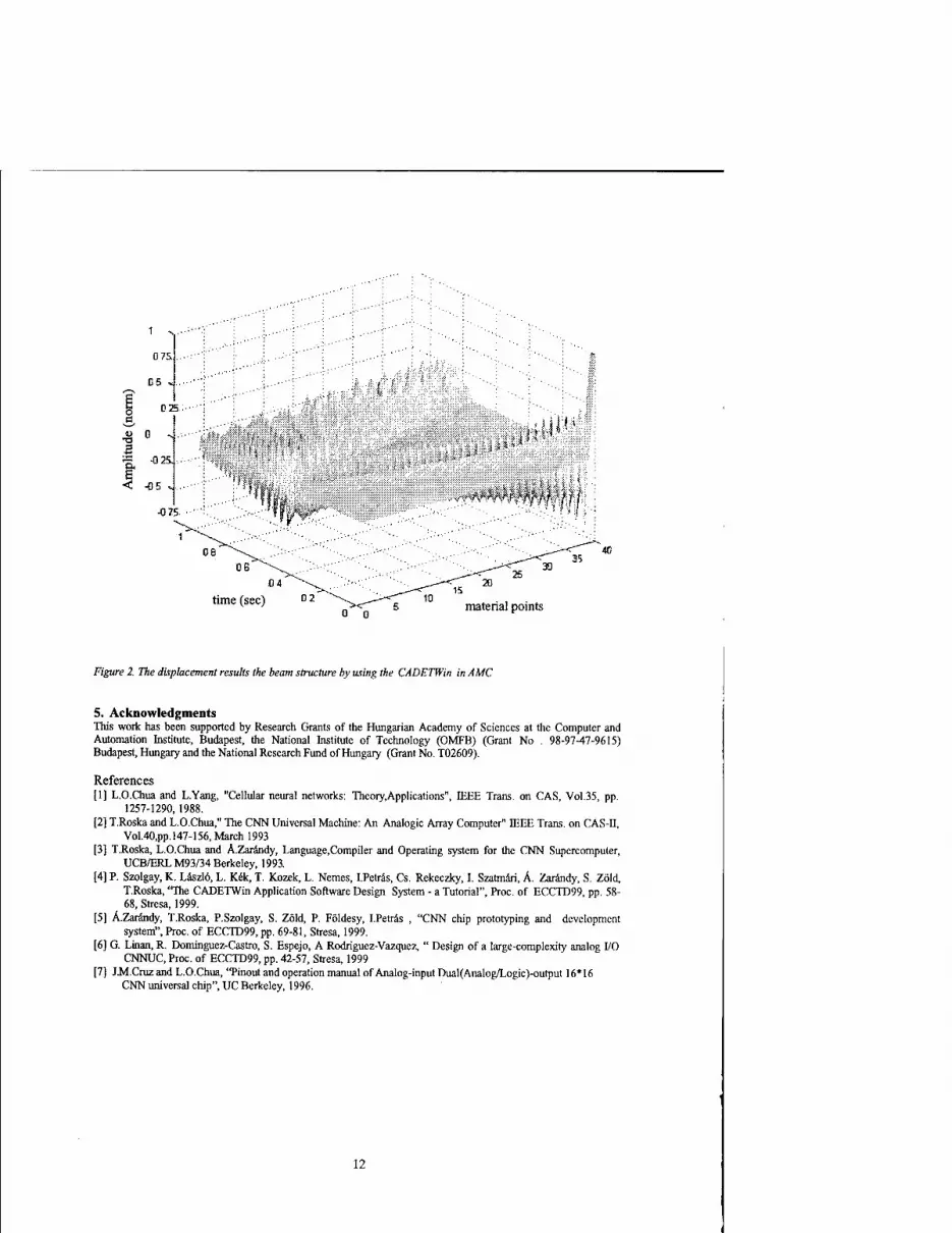
figure 2. 7%e displacement results the beam structure by using the CADETWin in AMC

5. Acknowledgments This work has been supported by Research Grants of the Hungarian Academy of Sciences at the Computer and Automation Institute, Budapest, the National Institute of Technology (OMFB) (Grant No . 98-97-47-9615) Budapest, Hungary and the National Research Fund of Hungary (Grant No. T02609).

References [1] L.O.Chua and L.Yang, "Cellular neural networks: Theory.Applications", IEEE Trans, on CAS, Vol.35, pp.

1257-1290, 1988. [2] T.Roska and L.O.Chua," The CNN Universal Machine: An Analogic Array Computer" IEEE Trans, on CAS-II,

Vol.40,pp.l47-156, March 1993 [3] T.Roska, L.O.Chua and A.Zarändy, Language.Compiler and Operating system for the CNN Supercomputer,

UCB/ERL M93/34 Berkeley, 1993. [4] P. Szolgay, K. Läszlö, L. Kek, T. Kozek, L. Nemes, I.Petras, Cs. Rekeczky, I. Szatmäri, A. Zarandy, S. Zöld,

T.Roska, 'The CADETWin Application Software Design System - a Tutorial", Proc. of ECCTD99, pp. 58- 68, Stresa, 1999.

[5] A.Zarandy, T.Roska, P.Szolgay, S. Zöld, P. Földesy, I.Peträs , "CNN chip prototyping and development system", Proc. of ECCTD99, pp. 69-81, Stresa, 1999.

[6] G. Linan, R. Dominguez-Castro, S. Espejo, A Rodriguez-Vazquez, " Design of a large-complexity analog I/O CNNUC, Proc. of ECCTD99, pp. 42-57, Stresa, 1999

[7] J.M.Cruz and L.O.Chua, "Pinout and operation manual of Analog-input Dual(Analog/Logic)-output 16*16 CNN universal chip", UC Berkeley, 1996.

12

[8] P. Szolgay, G.Vörös and Gy. Eröss," On the applications of the Cellular Neural Network (CNN) paradigm in mechanical vibrating systems", EEEE Transactions on Circuits and Systems Vol.40,pp. 222-227,1993.

[9] P.Szolgay, T Szabö, "On the detection of critical frequencies of a tool machine", Proc of IEEE CNNA'96, Seville, 1996

[10] P.Szolgay, I. Sälyi, Zs. Szolgay," Toward the application of an analog input dual output CNNUM chip in transient analysis of mechanical vibrating systems", Proc. of the IEEE INES97, Budapest, 1997.

[11] P.Keresztes, A. Zarandy, T.Roska, P. Szolgay, T.Bezak, T. Hidvegi, P. Jonas, A. Katona, " An emulated digital CNN implementation", J. of VLSI Signal Processing, Vol. 23, pp. 291-303, (1999)

13

2000 6™ IEEE International Workshop on Cellular Neural Networks and Their Applications Proceedings

NEUROMORPHIC CNN MODELS FOR SPATIO-TEMPORAL EFFECTS MEASURED IN THE INNER AND OUTER RETINA OF TIGER SALAMANDER

Csaba Rekeczky*, BotondRoska, Erik Nemetk*, and Frank Werblin*

'Analogical and Neural Computing Laboratory, Computer and Automation Institute, Hungarian Academy of Sciences, H-l 111 Budapest, Kende u. 13-17, Hungary

^Vision Research Laboratory, Department of Molecular and Cell Biology, University of California at Berkeley, Berkeley, CA 94720, USA

ABSTRACT: In this paper, a vertebrate retina model is described based on a cellular neural network (CNN) architecture. Though largely built on the experience of previous studies ([5], [11], [14]-[15], [17]-[18]) the CNN computational framework is considerably simplified: first order RC cells are used with space-invariant nearest neighbor interactions only. All nonlinear synaplic connections are monotonic continuous functions of the pre-synaptic voltage. Time delays in the interactions are continuous represented by additional first order cells. The modeling approach is neuromorphic in Us spirit relying on both morphological and pharmacological information. However, the primary motivation lies in fitting the spatio-temporal output of the model to the data recorded from biological cells (tiger salamander). In order to meet a low complexity (VLSI) implementation framework some structural simplifications have been made and large neighborhood interaction (neurons with large processes), furthermore the inter-layer signal propagation are modeled through diffusion and wave phenomena. This work presents novel CNN models for the outer and some partial models for the inner (light adapted) retina.

Introduction A cellular neural network (CNN, [l]-[5]) based vertebrate retina model is discussed synthesized from

morphological, pharmacological and physiological measurements. Contrary to a number of previous studies this work puts the focus on reproducing the spatio-temporal patterns of different biological cell layers in a low complexity CNN implementation framework instead of a phenomenological modeling of various retinal functionality (e.g. [17]-[18]). Trying to exactly determine the level of abstractness of the presented model, we can enunciate that following a neuromorphic approach either the cell level dynamics or the aggregate dynamics of a neural network is modeled. In this sense, the current work can be regarded as a continuation and extension of the comprehensive study by Jacobs et al. [15] since the motivation and the methodology used are similar. On the other hand, relying on recent physiological recordings from all discussed retinal cell types made possible to go beyond preceding results and create novel models for the outer and inner retina in a simplified CNN framework.

There are several strong arguments to justify why the CNN computational framework was chosen. The retinal cells are organized into layers, process analog signals and interact locally. Similarly, a CNN is composed Of planar arrays of mainly identical dynamical elements and the program of the entire network is determined by the strength (weights) of the local interactions. In this work the primary motivation was to built a retinal model on a level of abstraction that also defines a realizable physical architecture in the foreseeable future using an existing technology (VLSI, optical or quantum implementation). The main inter-cell interactions in the inner and outer retina are shown in Fig. 1.

Figure 1 Inter-cell interactions in the outer and inner plexiform layer, (left) schematic of the outer retina containing a cone photoreceptor, a horizontal and a bipolar cell, (right) schematic of the inner retina with bipolar cells, narrow field and wide field amacrine cells (ganglion cells that are driven by both bipolar terminals are not shown).

0-7803-6344-2/00/$10.00 ©2000 IEEE 15

The primary motivation of this study lies in building a neuromorphic network that can reproduce the spatio- temporal patterns recorded (see a qualitative approach focusing on functionality in [21]). However, if this is completed in a computational framework that defines a feasible physical architecture then biological-modeling efforts might gain an engineering profit. In the course of this work we tried to balance these two criteria and applied some restrictions to the CNN implementation framework to bring the models within the scope of the existing technologies.

According to the above reasoning the CNN computational framework is defined as follows: a) the base units are first order linear RC cells b) all inter-cell interactions are space-invariant and within a layer restricted to the nearest neighbors c) the synaptic characteristics are monotonic continuous functions d) the time delay in the interactions is continuous

The CNN retina model has been decomposed into functionally different sub-models in order to exactly identify the processing stages present and at the same time minimize the number of layers necessary for the implementation (see Fig. 2).

INPUT: Light

Cone-Horizontal models

Bipolar models

3 Neuron Disinhibitory Pathway

Trigger events

Wide-field activity

Ganglion models

OUTPUT to LGN

Figure 2 Decomposition of the CNN retina model into functionally different sub-models. The main building blocks of the outer plexiform layer (OPL) and the inner plexiform layer are shown (IPL). The OPL receives the light input and excites the IPL through the ON and OFF pathway. The IPL generates the final retinal output forwarded to the LGN (optic tectum of a salamander).

/. Observation, measurement, and estimation of the feature parameter set

v(m)(x,t) Fourier decomposition (IB)

SALAMANDER

RETINA

new parameter setting Simplex and combinatorial F = F(£^ E'J*i = VX. II AE I

optimization %

II. Model synthesis and optimization through parameter tuning

Figure 3 Flowchart of the modeling approach. Fourier decomposition of the spatio-temporal data was used to estimate the feature parameters (Fourier coefficients). The error function was calculated as a weighted squared difference of the feature parameters and a combined simplex-combinatorial search was employed tuning the model parameters.

16

The outer plexiform layer (OPL) is divided into the Cone-Horizontal and Bipolar blocks. The first one receives the light input and forwards a processed signal to the latter one. The Bipolar ON and OFF pathways are treated differently in the Bipolar sub-models. The main block of the inner plexiform layer (IPL), driven by the ON and OFF pathway of the outer retina, is the three-neuron disinhibitory pathway ([16], 3NDP: makes assumptions on connectivity and interactions of the bipolar terminals, narrow-field and wide-field amacrine cells). Trigger events corresponding to spatio-temporal changes at the bipolar terminals and the wide-field activity have been developed as independent sub-models. The block of the Ganglion models contains the interactions of the bipolar terminals and different amacrine cells with the ganglion cells. This block receives input signals from the 3NDP sub-model and generates the final retinal output forwarded to the LGN (optic rectum of a salamander). Synthesis, analysis and validation of a neuromorphic CNN model goes through several steps as shown in Fig. 3.

Spatio-temporal Patterns in the Outer Retina In this section the outer retina will be discussed, more specifically the focus is put on the interaction of cones,

horizontal cells and bipolar cells in the outer plexiform layer (OPL). Relying on I-V curve measurements (Fig. 4) and perforated patch clamp spatio-temporal recordings the modeling experiments lead to the following conclusions: (a) A second order nonlinear approximation seems essential to reproduce the underlying dynamics of all

measured cell responses. (b) There is no evidence supporting the hypothesis of a feedforward synoptic connection from the horizontal

to the bipolar cells, since abolishing this interaction can closely approximate all bipolar cell recordings. (c) At a light adapted state examined the horizontal feedback to the cones has a minimal influence in shaping

the spatio-temporal cone responses suggesting that the observed biasing and antagonistic effect of the horizontal cells influencing the bipolar output is mediated through a modulated synapse (the horizontal cells "modulate" the cone-bipolar and possibly the cone-horizontal transfer functions instead of directly affecting the cone membrane potential).

Cone l-V curves at different times Bjpolar_ON l-Vcurves at tfrfferent times

-■—•aomaad1

-•— '«msBtf ~A 'S0ms«f -▼— 75 m»?

-110 -100 -so

voltage (m\fl Voltage(mV)

Figure 4 Some measured I-V curves in the outer plexiform layer (recorded by Botond Roska). (le&) measured I-V curves at different times for the cone photoreceptors, (right) measured I-V curves at different times for bipolar ON cells (the curves are very similar for the OFF cells). Observe that both characteristics are nonlinear and changing in time above -40 mV. No recorded data is available for the horizontal cells since those cannot be clamped to a constant reference potential due to their large spatial extension.

There is no clear evidence for a feedforward synaptic connection from horizontal cells to bipolar cells. Though two recent reports ([7], [8]) suggest that the pathway might exist this has not been generally accepted in neurobiology [9]. It seems that there is enough evidence that the feedback pathway is sufficient to account for all antagonistic effects (see a summary in [11]). Contrary to some previous approaches (e.g. [14]-[15]]), in the current modeling experiments the feedforward pathway was completely ruled out in all network configurations and the spatial interaction was reduced to the nearest neighbors and monotonic continuous synaptic characteristics. We have shown that the spatio-temporal patterns of the simulation closely fit to the recorded data if second order nonlinear cell models are used corresponding to the measured I-V curves.

Fig. 5 illustrates the base model of the outer plexiform layer. Each biological cell layer is mapped onto a CNN layer that consists of first or second order cells. Typical values for the cell membrane resting potentials (£ra,) are given that determine the initial state values of all CNN cells (vc(0), vH(0), vB(0)). Solid lines represent excitatory, dashed lines inhibitory chemical synapses. The corresponding reversal potential (£,) values are shown at the arrows of the synapses (in a CNN model the a priori knowledge of the reversal potential values and the expected dynamic range of the cell membrane potential determines whether an interaction is excitatory or

17

inhibitory, i.e. whether the signal transfer is positive or negative, respectively). The inter-layer electrical coupling is marked by a circle and the strength is reflected by the value of the space constant (A.). In a light adopted retina it is assumed that the rods are saturated and "silent" therefore in the photoreceptor layer only the cones are modeled. The cones receive the light input and make excitatory connection to the horizontal and bipolar cells. In general it has been assumed that the cones receive a direct feedback inhibitory signal from the horizontals (gHC * 0) and there is no feedforward inhibition from the horizontal to the bipolar cells (gm = 0). All post-synaptic conductance functions (g) are monotonic (either decreasing or increasing) functions of the pre-synaptic potential (see the details in [19]).

OPL

Cone

Horizontal

Bipolar

Input: Light

-40

-35

-SO

Figure S The base model of the outer plexiform layer (OPL). Each biological cell layer is mapped onto a CNN layer that consists of first or second order (two mutually coupled first order) cells. Some conclusions and conjectures of the modeling experiments are also illustrated: (i) the forward pathway, from the horizontal cells to the bipolar cells, can be ruled out (dashed line gHB) and (ii) the horizontal feedback is rather a transfer function modulation (see the dash- dotted lines) than a direct effect on the cone membrane potential (dashed line gHc)-

Ceil responses In time (-r: Sim. ~b : meas) Can responses In üme (

1 Cell responses In time (-r: slm, ~b: meas)

0.5

0

-0.5

(c) (d) Figure 6 Comparison of the model output to the measured data for all four cell types of the outer retina (temporal responses are shown from three neighboring cells located in the middle of the stimulus: red solid lines: simulation; dashed blue lines: measurement, recorded by Botond Roska). All cell models are of second order and there is a slight feedback from the horizontal cells to the cones, (a) cone, (b) horizontal (average of the first two cells), (c) bipolar ON, (d) bipolar OFF.

Comparison of the model output to the experimental data suggests that the second order models are detailed enough to closely match the spatio-temporal transients observed in the physiological recordings. A temporal comparative analysis for the entire OPL composed of second order cells is demonstrated in Fig. 6. See further spatio-temporal recordings and simulation results in [19].

18

Wide-field Activity in the Inner Retina

In this section a CNN model of the so-called wide-field activity is discussed observed in the wide-field amacrine cells of the inner retina. The schematic of the interactions in the inner plexiform layer is shown in Fig. 1. Wide-field amacrine cells fire one spike at ON and OFF followed by a slow decay in response. Wide-field cells have long processes (up to 500 |im) and contain glycine (see a morphological, pharmacological and physiological correlation in [12]). These amacrine cells have a transient response since they receive excitatory inputs (from the bipolar terminals) near their somas and generate action potentials that propagate along the processes [13]. Neurotransmitter (glycine) release is a function of the changing presynaptic potential (it integrates the spiking) and generates a transient lateral inhibition, a "cloud" of activity, in the inner plexiform layer [10]. We have shown how the initiation and propagation of this activity can be properly modeled in the CNN framework [19].

Wide-field activity

fgTl

-80

/ < £l

(a) (b) Figure 7 (a) A three-layer CNN model of the wide-field amacrine cell activity. The model is excited by trigger signals of both bipolar terminals (up). Consequently, trigger waves will be generated on the first and second layer (the output of the first layer represents the wide-field activity). The third layer controls the spatio-temporal properties of the trigger-waves (tj < T2 « T3) with a smoothly and slowly changing output signal. A proper mutual coupling in between the second and third layer ensures that the spatial extension and the duration of the generated wide-field activity can be programmed without spoiling a unique feature of the model, i.e. it is capable of resetting itself without any external control, (b) Wide-field activity simulation results: a snapshot of 16 frames shown in 3D (left-to-right, up-to-down). Observe that the pattern is constrained both in space and time. The model exhibits a quick collapse from the center and a slow deactivation from the contour.

As mentioned earlier by wide-field activity we mean the integration of the action potentials along the wide- field amacrine cell processes. A nearest neighbor CNN model of the wide-field activity, described by Jacobs et al. [15], uses two layers for action potential generation (the simplified Hodgin-Huxley model must be at least of second order), four layers to model the electrical coupling between the compartments and an additional layer to integrate the action potentials. Action potential generation is solved by nonlinear templates, while the electrical coupling between the compartments is implemented by space-variant linear templates. The approach taken is truly neuromorphic, since exploring both the anatomical and physiological observations a biologically faithful model was designed. However, this model exceeds the complexity of the CNN framework set in the introduction since seven layers are used and space-variant programming of the network is necessary. Focusing on the output of the model one may realize that from signal processing point of view only a proper generation of a broadly extended transient lateral inhibition (the cloud of activity) is important. Here we will demonstrate that a significantly simplified three-layer CNN model based on space-invariant templates can reproduce this activity pattern, constrained both in space and time.

Physiological recordings suggest a simple characterization of the spatio-temporal wide-field activity: it is a traveling wave with a nearly constant amplitude that initiates at a bipolar terminal (around the soma of the wide- field amacrine cell) and activates the inner retinal regions up to a distance of 500 Jim (the maximum length of the amacrine cell processes) for a period less than 200 msec (150 msec is a typical value [16]). In [15] the timing is solved by explicitly modeling the action potentials and the spatial limit is introduced through space-variant templates that can describe the branched processes within a layer. In the current approach we present an entirely different solution (see Fig. 7(a)). Imagine that a "trigger event" initiates traveling waves on two separate layers, but the wave-fronts expand at a different speed. The quicker layer interacts with a third (control) layer that in turn solves the spatio-temporal timing of trigger waves through a continuous control of the activation threshold of all cells in both the first and second layer (details can be found in [19]). This model is regenerative, it returns to its initial state therefore re-triggering is also possible (Fig. 7(b)).

19

Within the framework set in the introduction, sub-models (Fig. 2) generating spatio-temporal trigger events and the corresponding wide-field amacrine cell activity (relying on the above described base model) were designed. In addition, a three-neuron serial pathway [16] of the inner plexiform layer was also synthesized [19] as a partial inner retina model (ganglion cells are not included). The output of these modeling blocks can be combined to form various ON, OFF and ON-OFF ganglion cell responses and makes it possible to study the global functional properties of retinal "image processing" ([19], [21]).

Conclusions

We have designed and analyzed novel CNN based models of the outer and inner retina based on morphological, pharmacological and physiological information. Compared to previous studies, a significantly simplified neuromorphic computational framework was used and a methodology developed that optimizes the network parameters fitting the output of the model to the recorded data (spatio-temporal patterns).

References

[I] L. O. Chua and L. Yang, "Cellular Neural Networks: Theory and Applications", IEEE Tram, on Circuits and Systems, Vol. 35, pp. 1257-1290, Oct. 1988.

[2] L. 0. Chua, and T. Roska, "The CNN Paradigm", IEEE Trans, on Circuits and Systems, Vol. 40, pp.147-156, March 1993.

[3] T. Roska and L. O. Chua, "The CNN Universal Machine", IEEE Trans, on Circuits and Systems, Vol. 40, pp. 163-173, March 1993.

[4] T. Roska and L. O. Chua, "Cellular Neural Networks with Non-linear and Delay-type Template Elements and Non- uniform Grids", Int. Journal of Circuit Th. andAppI., Vol. 20, pp. 469-481, 1992.

[5] F. S. Werblin, T. Roska, and L. O. Chua, "The Analogic CNN Universal Machine as a Bionic Eye", International Journal of Circuit Theory and Applications, Vol. 23, pp. 541-569, 1995.

[6] Cs. Rekeczky, T. Roska, and A. Ushida, "CNN-based Difference-controlled Adaptive Nonlinear Image Filters", International Journal of Circuit Theory and Applications, Vol. 26, pp. 375-423, 1998.

[7] W. A. Hare and W. G. Owen, "Spatial Organization of the Bipolar Cell's Receptive Field in the Tiger Salamander Retina", Journal of Physiology, 421, pp. 233-245, 1990.

[8] S. M. Wu, "Feedforward lateral Inhibition in Retinal Bipolar Cells: Input-Output Relation of the Horizontal Cell Depolarizing Bipolar Cell Synapse", Proc. Natl. Acad. Sei., 88, pp. 3310-3313, 1991.

[9] E. A. Kandel, J. A. Schwartz, and T. M. Jessell (editors), Essentials of Neural Science and Behavior, Prentice Hall International Inc., 1995.

[10] F. S. Werblin, "Synaptic connections, receptive fields, and patterns of activity in the tiger salamander retina", Investigative Ophthalmology and Visual Science, 32, pp. 459-483, 1991.

[II] F. S. Werblin, "Retinal Design: Using Physiological Measurements to Design a Complete Functional Real-time Retinal model", MCB164, Department of Molecular and Cell Biology, Division of Neurobiology, University of California at Berkeley, Spring 1994.

[12] Y. Yang, P. D. Lukasiewicz, G. Maguire, F. S. Werblin, and S. Yazulla, "Amacrine Cells in the Tiger Salamander Retina: Morphology, Physiology and Neurotransmitter Identification". Journal of Comparative Neurology, 312, pp. 19-32, 1991.

[13] P. B. Cook and F. S. Werblin, "Spike Initiation and Propagation in Wide-field Transient Amacrine Cells of the Salamander Retina", Journal ofNeitroscience, 14, pp. 3852-3861, 1994.

[14] J. Teeters, A. Jacobs, and F. S. Werblin, "How Neural Interactions Form Neural Responses in the Salamander Retina", Journal of Computational Neuroscience, Vol. 4, pp. 5-27, 1997.

[15] A. Jacobs, T. Roska, and F. S. Werblin, "Methods for Constructing Physiologically Motivated Neuromorphic Models in CNNs", International Journal of Circuit Theory and Applications, Vol. 24, pp. 315-339, 1995.

[16] B. Roska, E. Nemeth, and F. S. Werblin, "Response to Change is Facilitated by a Three-Neuron Desinhibitory Pathway in Tigger Salamander Retina", The Journal of Neuroscience, Vol. 18, pp. 3451 -3459, May 1998.

[17] T. Roska, J. Hämori, E. Labos, K. Lotz, L. Orz6, J. Takacs, P. L. Venetianer, Z. Vidnyanszky, and A. Zarändy, "The Use of CNN Models in the Subcortical Visual Pathway", IEEE Trans, on Circuits and Systems-I: Fundamental Theory and Applications, Vol. 40, No. 3, pp. 182-195, March 1993.

[18] K. Lotz, A. Jacobs, J. Vandewalle, F. Werblin, T. Roska, Z. Vidnyanszky, and J. Hämori, "Some Cortical Spiking Neuron Models Using CNN", International Journal of Circuit Theory and Applications, Vol. 24, pp. 301-314, 1996.

[19] Cs. Rekeczky, B. Roska, E. Nemeth, M. Wang, T. Roska, and F. Werblin, "The Network Behind Dynamic Spatio- temporal Patterns: Building Low-complexity Retinal Models in CNN Based on Morphology, Pharmacology and Physiology", DNS-7-I998, Technical Report, ANCL-HAS, Budapest, October 1998.

[20] A. Bouzerdoum and R. B. Pinter, "Shunting Inhibitory Cellular Neural Networks: Derivation and Stability Analysis", IEEE Transactions on Circuits and Systems, Vol. 40, pp. 215-221, 1993.

[21] D. Bälya, T. Roska, B. Roska, and F. Werblin, "A Qualitative Model for Spatio-temporal Effects in Vertebrate Retinas", in Proc of CNNA'2000.

20

2000 6™ TERR International Workshop on Cellular Neural Networks and Their Applications Proceedings

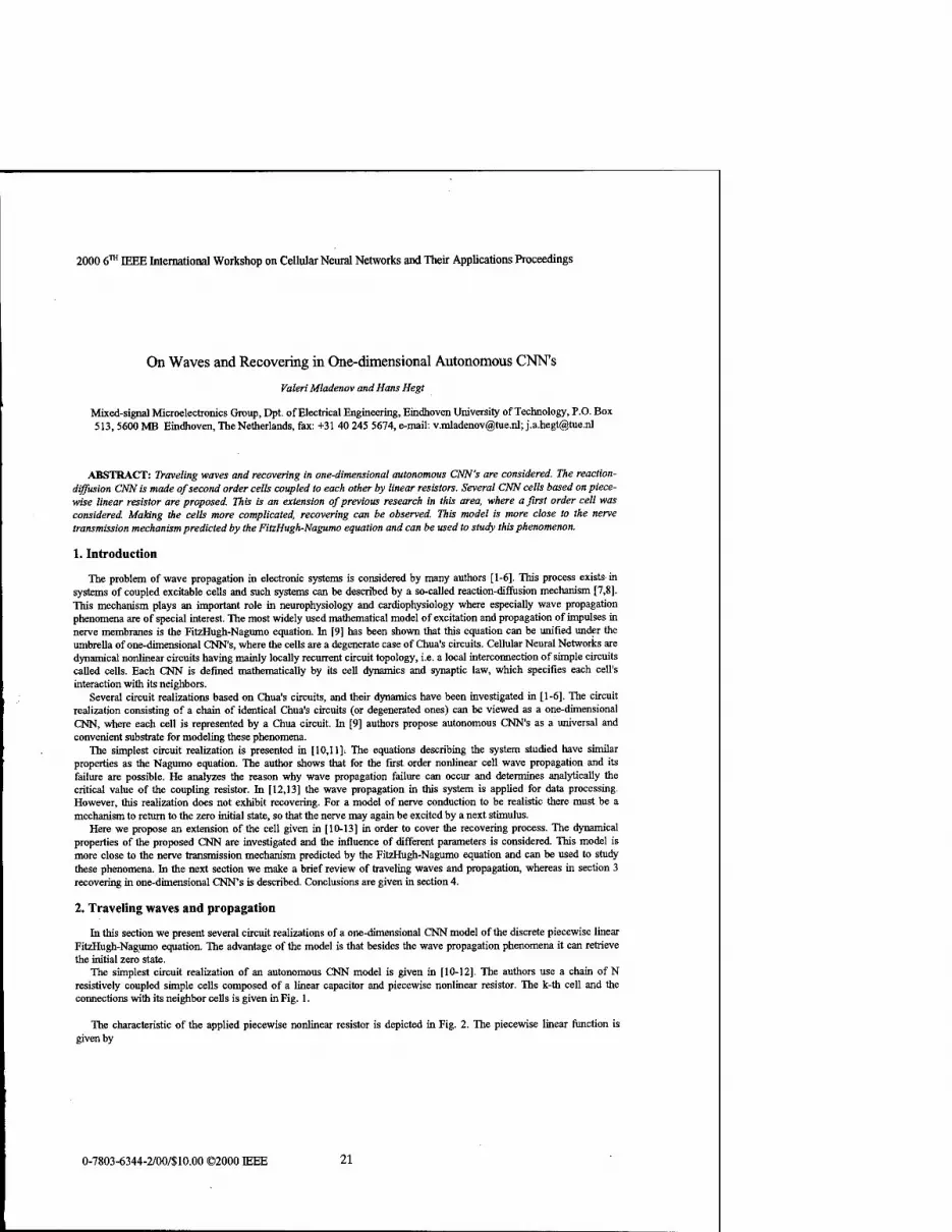
On Waves and Recovering in One-dimensional Autonomous CNN's

Valeri Mladenov and Hans Hegt

Mixed-signal Microelectronics Group, Dpt. of Electrical Engineering, Eindhoven University of Technology, P.O. Box 513,5600 MB Eindhoven, The Netherlands, fax: +31 40 245 5674, e-mail: v.mladenov@tue.nl; j.a.hegt@tue.nl

ABSTRACT: Traveling waves and recovering in one-dimensional autonomous CNN's are considered. The reaction- diffusion CNN is made of second order cells coupled to each other by linear resistors. Several CNN cells based on piece- wise linear resistor are proposed. This is an extension of previous research in this area, where a first order cell was considered. Making the cells more complicated, recovering can be observed. This model is more close to the nerve transmission mechanism predicted by the FitzHugh-Nagumo equation and can be used to study this phenomenon.

1. Introduction

The problem of wave propagation in electronic systems is considered by many authors [1-6]. This process exists in systems of coupled excitable cells and such systems can be described by a so-called reaction-diffusion mechanism [7,8]. This mechanism plays an important role in neurophysiology and cardiophysiology where especially wave propagation phenomena are of special interest. The most widely used mathematical model of excitation and propagation of impulses in nerve membranes is the FitzHugh-Nagumo equation. In [9] has been shown that this equation can be unified under the umbrella of one-dimensional CNN's, where the cells are a degenerate case of Chua's circuits. Cellular Neural Networks are dynamical nonlinear circuits having mainly locally recurrent circuit topology, i.e. a local interconnection of simple circuits called cells. Each CNN is defined mathematically by its cell dynamics and synaptic law, which specifies each cell's interaction with its neighbors.

Several circuit realizations based on Chua's circuits, and their dynamics have been investigated in [1-6]. The circuit realization consisting of a chain of identical Chua's circuits (or degenerated ones) can be viewed as a one-dimensional CNN, where each cell is represented by a Chua circuit. In [9] authors propose autonomous CNN's as a universal and convenient substrate for modeling these phenomena.

The simplest circuit realization is presented in [10,11]. The equations describing the system studied have similar properties as the Nagumo equation. The author shows that for the first order nonlinear cell wave propagation and its failure are possible. He analyzes the reason why wave propagation failure can occur and determines analytically the critical value of the coupling resistor. In [12,13] the wave propagation in this system is applied for data processing. However, this realization does not exhibit recovering. For a model of nerve conduction to be realistic there must be a mechanism to return to the zero initial state, so that the nerve may again be excited by a next stimulus.

Here we propose an extension of the cell given in [10-13] in order to cover the recovering process. The dynamical properties of the proposed CNN are investigated and the influence of different parameters is considered. This model is more close to the nerve transmission mechanism predicted by the FitzHugh-Nagumo equation and can be used to study these phenomena. In the next section we make a brief review of traveling waves and propagation, whereas in section 3 recovering in one-dimensional CNN's is described. Conclusions are given in section 4.

2. Traveling waves and propagation

In this section we present several circuit realizations of a one-dimensional CNN model of the discrete piecewise linear FitzHugh-Nagumo equation. The advantage of the model is that besides the wave propagation phenomena it can retrieve the initial zero state.

The simplest circuit realization of an autonomous CNN model is given in [10-12]. The authors use a chain of N resistively coupled simple cells composed of a linear capacitor and piecewise nonlinear resistor. The k-th cell and the connections with its neighbor cells is given in Fig. 1.

The characteristic of the applied piecewise nonlinear resistor is depicted in Fig. 2. The piecewise linear function is given by

0-7803-6344-2/00/S10.00 ©2000 IEEE 21

uk-1 R "• VWW"

R -wvw- "k+1

Cd= |tf<uk>

Figure 1: One-dimensional array of resistively coupled circuits suggested in [10-12].

f-0.25«,, «,-<0.2

/(u,) = jo.25u,-0.1, 0.2<u,£0.8

-0.5«, +0.5, u, >0.8

(0

Pi»c*wi9* linear characteristic of th« rton-lin«ar resistor

2 -01 0 01 02 0.3 04 05 06 07 08 09 1 11 1.2

Figure 2: Piecewise linear resistor considered in [10-12].

As in [10-12], the regions appearing in (1) will be referred to as {1}, {2} and {3} for u <0.2,0.2 <,u <,Q.8 and u >0.8

respectively. The slopes of function/^ in each of the three regions will be denoted as

m = — ,

where the superscript r indicates the corresponding region. The dynamics of the above model can be described by a set of N first order differential equations

,dut

dt = rf(«^,-2«t+«ttl) + /(«A), * = 1,2,...,JV (2)

where d = — is the conductance of the coupling resistors. Because C can be treated as a time scaling parameter, set C= 1. R

In [10-12] the author considers zero flux boundary conditions, yielding u, =«0 and uN =uNt] and investigates the

dynamic behavior of the model. He proves that in the case of traveling wave propagation a heteroclinic orbit does exist in the associate continuous system and analyses the reason why wave propagation failure can occur. Furthermore, the author determines the critical value of the coupling resistor.

22

As was mentioned before, this model suffers of missing a recovering mechanism. That means that, in the case of traveling wave propagation when all cells are excited, there is no internal mechanism to retrieve the cells in the zero initial state. Because of this, the cells could not be excited again and the model is not appropriate for detailed modeling of the nerve transmission mechanism.

In this paper, we consider an autonomous CNN model described by the following system of equations

du ^ = rf(«t_,-2«t+«4+,) + /(«t)-wi, * = l,2,...,tf

ut

dt v * *

(3)

where f(ut) is given by (1). Normally e ->0 and wh k=],2,...,N become slow variables with respect to uh k=l,2,...,N. The considered model is a discrete version of the FitzHugh-Nagumo equation [7], [9]. This is a more realistic model of nerve conduction because of the presence of slow variables wh k=],2....,N, which give an internal mechanism for recovering. We introduce several circuit realizations of the basic cell. The k-th cell and the connections with its neighbors for the different realizations are given in Figure 3a, 3b and 3c. In these cases (p(uk) are different piecewise linear

functions such that the resulting nonlinear function/fa^) in (3) is the same as given by (1).

« VWVk—

—*f<1—, uk

—WW *-

R0 ^<^ = co

Cr " |TKV

Rl 1 VWA

Figure 3a R

-WWr-

-WWV-

-WMr Ro

"Co

r -WW\r-

R -wwv-

Figure 3b

C^= gt,'<ul<)

Figure 3c

Figure 3: Several circuit realizations of the presented autonomous CNN for a discrete version of the piecewise linear FitzHugh-Nagumo equation.

It should be pointed out again that when £ ->0,ut, t=/,2,...,Ware fast variables wfc k=],2,...,N are slow variables [1], [14]. Exploring the idea of different time scales [ 1 ], [ 14], one can observe that in the beginning of the transient after the first cell is excited the influence of wh k=l,2,...,N is negligible and equations (3) can be approximated by equations (2). Hence all considerations in [10-12] for wave propagation and its failure are applicable. In the case of propagation for a relatively large time, the influence of the slow variables wh k=l,2,...,N becomes considerable and may cause the return the system into the zero initial state.

23

3. Recovering in one-dimensional autonomous CNN's

In this section we will prove that the recovering is possible. In fact, we will prove the existence of solitary waves (see fig. 4c). Without the variables wh k=l,2,...,N, traveling waves are possible (see fig. 4a.) [10-12]. In the case of our model, the influence of the new (slow) variables wt , k=l,2,...,N, consists of the "transformation" of the traveling wave into a solitary wave. This "transformation" takes a relatively long time due to the fact that variables wh k=l,2,...,N arc "slow". During this time the cells are in excited mode and thereafter in unexcited mode (recovering).

First of all we will find the equilibrium points of system (3) and will prove their stability. The equilibrium points of the system considered are the solutions of the corresponding system of algebraic equations, when the right side of (3) is set to zero. One can observe that for b<8 this system has the unique equilibra (ut wh)=0, k=l,2 N . This is the case of interest for recovering. For b>8 the system has three equilibrium points and this does not guarantee the expected dynamics. To prove the stability of the equilibrium points, we will use the technique described in [15]. Here we will point out some basic steps. The main idea, used in [15], is to separate the spatial and temporal information after which the general form of the solution of (3) can be found as

hi

•2 _ («> W*(0 = 2A (U)w,(0,* = 1,2 N

1=1

where the N space dependant orthonormal functions <t>N (i, k) are spatial eigenfunctions of the discrete Laplacian

V 20„ (i, k) = fo„ (i, k +1) + <,„ (i, k -1) - 2<t>N (i, *)] = -pfyN (i, k) (5)

Here with k are denoted the numbers of the cells and i is the summation index. Taking into account the zero flux boundary conditions [15]

fff(i-l)> = 4sin'

N

MU) = ex|//^-(i-lX*-l)

The following N pairs (i=],2 TV) of linear differential equations can be obtained by substituting (4) into (3)

du, 2 — — = (m - pi d)ui - wi + const:

* (6) aw: — — ~eu, -ebw:

dt

where const,' depends on the working region (const/ =0, const,1 =-0.1 and const' =0.5 ) and ut and wk are spectra of

ukand wt with respect to the orthonormal basis {<j>N(i,k), i = \,2,...,N, k = \,2,...,N}.

The roots of the following equation give the temporal eigenvalues of system (6)

A2 +(eb + pfd -m')X + (p?d£b + £-m'cb) = 0

If the cells are in the regions {1) or (3}, ni<0 (equilibrium point is in region {1}), the eigenvalues have negative real parts, i.e. the system is stable.

To prove the existence of solitary waves we assume ut+1 + uk_l - 2uk = h2 —- and thus (3) is transformed into 312

du 2 3 " r, s — = dh + /(>')- dt a^ Jy

— = e(«-Mv) dt

(7)

Introducing the moving coordinate [1, 3, 6, 10, 11, 12] £ = t-kh, h > 0 and rewriting (7) with respect to this coordinate we get

w = v v=v w >- w = e(u-bw) (8) dh2

24

where the dot denotes differentiation with respect to \ Note that \ is the coordinate moving along the array with a

velocity llh. Solitary waves of the model considered correspond to nonconstant solutions of (8) wich satisffy the condition

Urn («(£), v(O,»-«)) = 0 W

Condition (9) is satisfied by the homoclinic orbits ([6], [ 16]) of system (8). This wave system has a unique equilibrium point (u,v,w)=(0,0,0) for b<8. The characteristic equation related to this equilibrium point is

-l}+(\/K-eb)X1+(eb/K-m/K)A+(E/K-Ebm/K) = 0,

where K = 1 / dh1 and m = -2-i!fl. For region {1}, in which this equilibrium point is located, m=-0.25 and it is easy to du

observe that the solution of this equation yields one positive real eigenvalue and two eigenvalues with negative real parts (because of the sign configuration of the coefficients). The equilibrium can be either saddle or saddle focus [16], with one- dimensional unstable manifold and two-dimensional stable manifolds. This is connected with a homoclinic orbit [16], which results in a solitary wave.

Simulation results of the dynamic behavior of models (2) and (3) are given in Figure 4. The traveling wave for model (2) for N=15, C=l, d=0.2 and ^=150 is given in Fig. 4a. (Fig. 3 from [12]). The solitary wave for model (3) with the same value of the parameters N, C, d, tr„ and £ = 0.0001, b=l is given in Fig. 4b. It is easy to observe the coincidence of the behavior of both models for tfi„=150. Fig. 4c shows the dynamic behavior of model (3), for tto=1500. The recovering process (solitary wave) retrieves the zero initial state of the system.

4. Conclusion

In this paper, the traveling wave and recovering in a one-dimensional autonomous CNN are considered. The reaction- diffusion CNN is made of second order cells coupled to each other by linear resistors. Several CNN cells based on piece- wise linear resistor are proposed. This is an extension of previous research in this area, where a first order cell was considered. Making the cells more complicated, the recovering can be observed. This mechanism is inherent to real nerves and thus the model helps to simulate and analyze more realistically its behavior.

5. References

[1] V.Perez-Munuzuri, V-Perez-Villar, L.O.Chua: "Travelling wave front and its failure in a one-dimensional array of Chua's circuits", J. Circuits and Comp., Vol. 3, No.l, pp. 211-215,1993. [2] A.P.Munuzuri, V.Perez-Munuzuri, M.Gomez-Gesteria, L.O.Chua, V-Perez-Villar: "Spatiotemporal structures in discretely-coupled arrays of nonlinear circuits: a review". Int. Journal Bifurcation and Chaos, Vol. 5, No. 1, pp. 17-50, 1995. [3] V.LNekorkin, L.O.Chua: "Spatial disorder and wave fronts in a chain of coupled Chua's circuit", Int. Journal Bifurcation and Chaos, Vol. 3, No. 5, pp. 1281-1291,1993. [4] V.LNekorkin, V.B.Kazantsev, L.O.Chua: "Chaotic attractors and waves in a one-dimensional array of modified Chua's circuits", Int. Journal Bifurcation and Chaos, Vol. 6, No. 7, pp. 1295-1317,1996. [5] V.LNekorkin, VE.Kazantsev, M.G.Velarde: "Travelling waves in a circular array of Chua's circuits", Int. Journal Bifurcation and Chaos, Vol. 6, No. 3, pp. 473-484, 1996. [6] V.LNekorkin, V.B.Kazantsev, M.F.Rulkov, M.G.Velarde, L.O.Chua: "Homoclinic orbits and solitary waves in a one- dimensional array of Chua's circuits", IEEE Trans. Circuits and Systems, Part I, Vol. 42, No. 10, pp. 785-801,1995. [7] J.P.Keener: "Propagation and its failure in coupled systems of discrete excitable cells", SIAM J. Appl. Math., Vol. 47, pp. 556-572, 1987. [8] T.Roska, L.O.Chua, D.Wolf, T.Kozek, R.Tetzlaff, F.Puffer: "Simulating nonlinear waves and partial differential equations via CNN - Part I: Basic techniques", IEEE Trans. Circuits and Systems, Part I, Vol. 42, No. 10, pp. 807-815, 1995. [9] L.O.Chua, M. Hasler, G.S.Moschytz, J.Neirynsk: "Autonomous cellular neural networks: a unified paradigm for pattern formation and active wave propagation", IEEE Trans. Circuits and Systems, Part I, Vol. 42, No. 10, pp. 559-577, 1995. [10] D.M.W.Leenaerts: "Wave propagation and its failure in piecewise linear Nagumo equations", Proc. European Conf. Circ. Theory and Design, Budapest, pp. 342-347,1997.

25

[11] D.M.W.Leenaerts: "On traveling waves in a one-dimensional array of resistively coupled cells", Proc. Int Symp NOLTA'97, Honolulu, pp. 257-260, 1997. [12] D.M.W.Leenaerts: "Data processing based on wave propagation". To appear in International Journal of Circuit Theory and Applications 1999. [13] D.M.W.Leenaerts, K.Doris: "Data processing using nonlinear wave propagation: the meta-stable state", Proc. Int. Symp. NOLTA'99, Hawaii, pp. 637-641, 1999. [14] P.Ortoleva, J.Ross: "Theory of propagation of discontinuities in kinetic systems with multiple timescales: Fronts, front multiplicity, and pulses", J. Chem. Phys., Vol. 63, pp. 3398-3408, 1975. [15] L. Goras, L.O.Chua: "Turing Patterns in CNN - Part II: Equations and Behaviors", IEEE Trans. Circuits and Systems, Part I, Vol. 42, No. 10, pp. 612-626, 1995. [16] Yu. A. Kuznetsov: "Elements of Applied Bifurcation Theory", Springer-Verlag, New-York, Berlin, Heidelberg, 1995.

Nagumo model Fit2Hugh-Nagumo model

1-,

08.

|D6-

1 504-

02-

■o,

1 I« I^T^^'J^1 '35 1fi0 15** cell number 120 135'l50*lri5 cellrtumbei

time

Figure 4a ;):</> »<*cr.ivf.i:*i

tim»

Figure 4b

T-^XU:ji-i'fh^-

läS «,:

Figure 4c

Figure 4: Simulation results of the behavior of models (2) and (3): a) the traveling wave for model (2) for N=15, C=l, d=0.2andtfl„=150; b) the solitary wave for model (3) for N=l 5, C=l, d=0.2, 1^=150, £ = 0.0001, b=l; c) the solitary

wavefor model (3)forN=15. C-l, d=0.2, tfl„=1500, E = 0.0001,ft=/

26

2000 6™ IEEE International Workshop on Cellular Neural Networks and Their Applications Proceedings

Phase Influence on Mode Competition in Turing Pattern Formation Liviu Gora$, Tiberiu Teodorescu, Andrei Maiorescu

Abstract Within linear theory, Turing patterns in CNN's can be viewed as the consequence of a competition between unstable spatial modes. The aim of this communication is to show that the final pattern might depend on the relative position (phase) of the competing modes - a result that cannot be explained using the mode decoupling linear theory.

INTRODUCTION

The two-grid coupled Cellular Neural Networks (CNN's) architecture [1-11] has been shown to be capable to produce Turing patterns on the basis of a mechanism similar to that proposed by Turing [14]. Composed of identical cells identically coupled by means of two homogeneous resistive grids, such CNN's exhibit an unstable homogeneous equilibrium point, which corresponds to a stable one for an isolated cell. The pattern is one of the stable equilibrium points towards which the network emerges. The linearized equations governing the dynamics of the array have the form:

du (t) , -ji2 = Y(fuu,i-rf¥va) + DHV

2us dt (1)

dva(t) dt

^(guUij+gvV^ + D^Vy

(2)

where/„ /„ g„ gv refer to the linearized two-port resistive characteristics (elements of the Jacobian matrix

of f(u,v) and g(u,v) of the nonlinear equations), D„ and Dv are the diffusion coefficients and V is the discrete Laplacian. The Turing conditions [3-8], that have been shown to be only necessary for discrete- arrays, are:

L + Sv < 0

Lg, - /.& > o DJU + Dugy > 0 (A,/„ " Dugvf + 4DuDJvgu > 0

Within linear theory, Turing Patterns in CNN's are dependent on the following aspects: a - fulfillment of Turing conditions,

b - dispersion curve,

c - initial conditions,

d - biasing sources signal [3] Beside, the shape of the nonlinear characteristic of the cell resistor influences the pattern as well but this is an aspect that cannot be consider within the above theory. However, it has been shown that the results of the linear theory fit well with the simulations mainly for ID arrays. In such cases, the final pattern can usually be predicted taking into consideration the above aspects, which means that the nonlinearity (f„(u) in most cases - as shown in Fig.l.) plays mainly the role of limiting the growing process of the unstable spatial modes.

fu(u) A

Fig. 1: A typical cell non-linear characteristic

0-7803-6344-2/00/S10.00 ©2000 IEEE 27

Using the decoupling technique, i.e., the change of variable

"/(')= X <t>u(m,i)am(t) (3)

i=0,l,.. .,M-1, where the functions <t> u (m, i) are dependent on the boundary conditions as shown in [5] In terms of the new variables, the dynamics of the CNN is described by the following set of pairs of decoupled linearized equations

«»(0

v»(0 .feu cv

Du 0

0 D„ uB(t)

v«(0. +7 0 (4)

The general form of the transient expressed in terms of the decoupled variables [9]

»m(t) = am(im,um(0),vm(0))e "> + bm(£m,um(0),vm(Q))e "^ +/,(em) (5)

[vm(t) = cm(im,um(Q),vm(0))e ""I +dm(im,üm(0),vm(0))e m2 + f2(i„)

where X^i and X^ are the roots of the characteristic equations

X2m +X*[k* CD. +Dv)-Y(fu +gv)]+DuD¥ki

-y(Dvf„ + Dugv)k* +(fugv -fvgu) = 0

and fi and fi are [9]

(6)

/l(£m) =

/2(e») =

-rQgy-ftmPy)

(If« - *»C« )(3Sv - 4»v) - /VvS« fju ^ (Tfu -klDu\ygv-klDv)-y

2fvgu '

(7)

(8)

The time domain solution of the 1-D linearized CNN equations is thus

M-l k ( x (

»i(0 = X(a«>(e»>'u'»(0)'Vj0))e mi +bm(Em,fim(0),vm(0))e m2 +f1(Em))0M(m,i)

M-l x , x t vi(0 = 2>„,(em.üm(0)>vm(0))c m' + dm(em,um(0),vm(0))e "^ +f2(Em))<I>M(m,i)

.271 .

For ring boundary conditions, the orthogonal basis of functions is: <J>M(nu)=e M and the corresponding

eigenvalues, k2m = 4sin2 —.

M The dispersion curve represents the real part of the temporal eigenvalues versus the spatial eigenvalues. A typical dispersion curve is represented in the figure below:

28

.-, 1 Re(t eigenvalue) _/r~j~

%i

M

•;• :

..• : t / I i v

/ II -"' ! 1 i, i i ' i i

modes ;:::;:

Fig. 2: A typical dispersion curve For the situation in the figure, there are two "active" modes: 4 and 5. We say that they are "inside" the dispersion curve, i.e. they have eigenvalues with positive real parts. When using non-homogeneous spatial bias current sources, the "spatial signal" made by bias current sources influence the solution. We stress the fact that the functioning point is before entering the non-linear part of each cell's characteristic.

PHASE INFLUENCE ON MODE COMPETITION

For initial conditions consisting of two pure spatial modes the technique of decoupling the differential equations predicts a race between the spatial modes which depends on their weight in the initial conditions and on the magnitude of the (positive) real parts of the corresponding temporal modes. The relative position of the two spatial modes is irrelevant within the linear theory. This statement is true as far as the amplification conditions for one mode are much more favourable than for the other one (in terms of amplitude ratio and eigenvalue real parts) [10-13]. However, when the competition is "tight", it has been found that the relative position (phase) of the two competing modes can influence the final pattern. The simulations have been done with the following parameters:

ID size

fu fv gu gv gamma du dv

50 0.4 1 -0.25 -0.5 1 1 10

Parameters deduced from the dipersion curve:

peak kl k2 Dvcrit kcrit m=l(TN) m=2(IN) m=3(IN) m=4(IN)

0.14864®

0.09325

0.01492 0.33508 3.2725 0.1236 0.0096®

0.0158

0.1401®

0.0628

0.1371®

0.1404

0.0705®

0.2474

The phase influences the final pattern in the non-linear way. That means we cannot say anything regarding the final pattern taking into account only the evolution in the linear part when we are talking about the influence of the phase. In order to prove the above-mentioned statements, we seed the network with the sum between mode 3 of amplitude 0.1 and phase pi/10 and mode 2 of amplitude 0.0905. The initial state, the evolution of the initial state to the final pattern and the final pattern are represented in the figure below. From the table it can be easily seen that mode 2 has the biggest real part for the temporal eigenvalue. Despite this, mode 3 will "win" the competition in the non-linear part. This is because of the influence of the phase:

29

Mt

\ ,! \ : : 1 \ !

/ N \ / : ' :\ I \ ■\

t \ /: : : \ 1

- ^Ä?5^ U.yj.%. \J-\J. .\l

Fig. 3: Initial state, Evolution to the final pattern, final pattern

In the second experiment, we seed the network with mode 3 and 2 of the same amplitude. The phase of the mode 3 is now pi/54. The result is that mode 2 will win the competition for phase smaller or equal than this value:

aj,mi ■ wmsm* \

....

\ ' 1 \

1 \ / 1 1

r-< ' ' \

—i

iggBjgmmmmmmmmmmmmmmmmmsm

Fig. 4: Initial state, Evolution to the final pattern, final pattern

Moreover, the position of the "breaking points" in the cell's characteristic does matter.

The left "breaking point" in the non-linear part of the cell's characteristic is -1 and the right "breaking point" is changed from 1 to 10. The phase of the mode 3 is zero in the following experiment:

mam

Fig. 5: Initial state, Evolution to the final pattern, final pattern We change the phase to pi/5500. The result can be seen in the figure below:

i

r\ P i\ \

\ / \ / / \ /:

', •t-j '": ""■*

.... ""■

~1 ■""( JB t> % » «

Fig. 6: Initial state, Evolution to the final pattern, final pattern From the Fig. 6 (final pattern) it can be seen that mode 2 distorted "wins" the competition.

30

Then we eliminate the distortion of the winner (mode 2) by changing the phase of the mode 3 to pi/10:

■I 1 4 i i \ 1 1-jL.ä

:IWi M ■ ^'^*

1 i : I !A : i -t-^i-

...XL

Fig. 7: Initial state, Evolution to the final pattern, final pattern In the next four experiments, we will emphasize another important aspect: it is possible to obtain a new different pattern corresponding to a different mode from the mode(s) with which we seed the network. The importance of the phase will be stressed, too. We will seed the network with a sum between modes 1 and 4 with different amplitudes. First, we use amplitude of 0.3 for mode 1 and 0.01 for mode 4. The phase is zero. Mode 2 will win the competition. Remark: in the initial spectrum composition: there wasn't mode 2 at all. This is up to the non- linearity.

44vi i m I I -i ntj -j/t | | ||

1? ■ ^■■■■^■■■H"'ii1"'X'"JiJ-"'i,,,*iiV;,T,ii !

! fix! I ! £j\!

Fig. 8: Initial state, Evolution to the final pattern, final pattern Then we change the amplitude of mode 1 to 0.2. The rest will be unchanged. Another mode that wasn't present in the initial spectrum wins the competition: mode 3:

",...'-.. 'ii % -. ~'

¥|T\ / \ / «c \ / \ / ^ \ /

\ • U v_ .

-~

;:::■:::::#£

■Uli lllllilllli^iiiiiiliiii:

•■•-.

Fig. 9: Initial state, Evolution to the final pattern, final pattern By slightly changing the amplitude of mode 1 to 0.1968, we obtain the pattern corresponding to the mode 4:

IM

A fa* BS "

/ i

:;;:a*:;$"ft*:mS;:**::*

9- f* w*^ av- :

H ntr; h tw iVi- t-w-! :Wi i-y-

Fig. 10: Initial state, Evolution to the final pattern, final pattern

31

Mode 3 can be obtained by changing the phase of mode 4 from 0 to pi/10:

\ li'lvA ■ \ ■ \ 'i M' >■

Fig. 11: Initial state, Evolution to the final pattern, final pattern

CONCLUDING REMARKS

In this work we have experimentally proved that the phase in a second order cell CNN can be crucial in the mode competition for Turing Pattern formation. For these situations the prediction of the final pattern according to the previous works based on mode decoupling techniques cannot be obtained. Moreover, new modes, other then the ones seeded into the network can appear as winners in the final pattern.

Equations and Behaviors", IEEE Trans.

Part III: Computer Simulation Results",

References [I] L. O. Chua, L. Yang, "Cellular Neural Networks: Theory", IEEE Trans. Circuits Syst., vol. 35, no 10, pp. 1257-1272, October 1988. [2] L. O. Chua, L. Yang, "Cellular Neural; Networks: Applications", IEEE Trans. Circuits Syst., vol. 35, no 10, pp 1273-1290, October 1988. [3] V. P. Munuzuri, M. G. Gesteira, A. P. Munuzuri, L. O. Chua, V. P. Villar, "Sidewall Forcing of Hexagonal Turing Patterns: Rhombic Patterns", Memorandum No. UCB/ERL M94/35, April 1994. [4] L. Gora$, L. O. Chua, D. M. W. Leenaerts, 'Turing Patterns in CNN's-Part I: Once Over Lightly", IEEE Trans. Circuits Syst, vol.42, pp. 602-611, October 1995. [5] L. Goras, L O. Chua, 'Turing Patterns in CNN's - Part II: Circuits Syst, vol.42, pp. 612-626, October 1995. [6] L. Goras, L. O. Chua, L. Pivka, 'Turing Patterns in CNN's IEEE Trans. Circuits Syst, vol.42, pp. 627-636, October 1995. [7] D. M. W. Leenaerts, L. Goras, L. O. Chua, "On the Properties of Turing Patterns in a Two-Cell CNN", Proceedings of the International Symposium on Signals, Circuits and Systems, SCS'95, Iasi, 19-21 October 1995. [8] L. Goras, L. O. Chua, Turing Patterns in CNN's Based on a New Cell, Proceedings of the Fourth International Workshop on Cellular, Neural Networks and Their Applications, Seville, Spain, June 24-26, 1996 [9] T. Teodorescu, V. Maiorescu, "Using Different Bias Current Sources for Controlling Turing Patterns", ECCTD'99 Proceedings, September, 1999, Stresa, Italy [10] L. Goras, L. O. Chua, Turing Patterns in CNN's Based on a New Cell, Proc. of the Fourth International Workshop on Cellular, Neural Networks and Their Applications, CNNA'96, pp. 103-108, Seville, Spain, June 1996. [II] L. Goras, L. O. Chua, On the Influence of CNN Boundary Conditions in Turing Pattern Formation, Proc. of the European Conference on Circuit Theory and Design, ECCTD, Budapest, 1997. [12] T. Teodorescu, L. Goras, On the Dynamics of Turing Pattern Formation in ID CNN's, Proceedings of the Int. Symposium on Signals, Circuits and Systems, SCS'97, Ia$i, October 1997. [13] L. Goras, T Teodorescu, " On CNN Boundary Conditions in Turing Pattern Formation", Proc. of the Fifth International Workshop on Cellular, Neural Networks and Their Applications, CNNA'98, pp. 112- 117, London, UK, 14-17 April, 1998. [14] A. M. Turing, "The Chemical Basis of Morphogenesis", Phil. Trans. Roy. Soc. Lond. B 237, pp.37-72, October 1952.

32

2000 6™ IEEE International Workshop on Cellular Neural Networks and Their Applications Proceedings

Dynamics of autowave processes in Neuron-like systems and CNN technology.

V. G. Yakhno

46 Ul'yanov Street, 603600 Nizhny Novgorod Institute of Applied Physics, Russian Academy of Sciences

E-mail: yakhno@appl.sci-nnov.ru

ABSTRACT: The most typical basic models of neuron-like media which describe both dynamics of homogeneous systems and hierarchic levels of recognition of complex images are considered. These models are analogous ones used in CNN technology. The results of studies of the possible dynamics of spatio-temporal (autowaves) structures are presented. The obtained solutions were used to interpret the dynamics of a normal perception modes and violations in the transformation of sensor signals in physiological experiments. Examples of the dynamics of parallel processing modes of a complex images and adaptive modes for making a decision systems are demonstrated.

1. Introduction

One of the most exciting mysteries of Nature is associated with the principles of constructing systems characterized by a wide range of adaptive reactions to various complex signals / images. These systems are made of universal elements (biomembranes, neurons, neuron ensembles, nervous tissues, etc.). The researchers have already obtained a lot of experimental data concerning characteristic reactions of adaptive elements at different levels of brain hierarchy, suggested mathematical models of neuron ensembles (which can be called "classical"), described key basic structures of collective activity of such distributed nonequilibrium media, found algorithms of distinguishing necessary informational features in a parallel regime, elaborated associative data bases, etc. However, when trying to unite the above data the researchers rely mainly on their intuition as there is no adequate "language" to describe excitation dynamics in such distributed media.

The AWP team working with IAP RAS have a long-year experience in this field that helped them to form a set of basic models of hierarchic neuron-like systems and to develop the methods to analyze possible collective activity structures, so called autowave processes (AWP), in distributed nonequilibrium neuron-like media.

2. Basic models for analysis neuron-like systems

We considered the main forms of data transformation in neuron-like systems required for adaptive recognition of complex images. Neuron-like systems are distributed systems or network architectures consisting of active elements with several stable (or "quasistable") states and nonlocal spatial couplings between such nonequilibrium elements (see, e.g., [1-8]. In designing adaptive systems, we proposed three levels for description of image- processing dynamics

To the first level we relate the models of homogeneous nonequilibrium neuron-like media with one, two, three or more components. Each component in such models (represented by integro-differential equations) is characterized by its particular scheme of active mechanisms, particular values of relaxational temporal parameters and type of spatial couplings (see, e.g., Fig. 1) [3, 15-17, 23-25]. A similar model for digital network of coupled neuron-like active units, known as the CNN paradigm, was examined in [18-22].

To the second level we relate the models of "elementary"' classifiers or decision-making systems with fixed algorithms and a set of operations required for classification of video images. If parallel modes of processing of given objects or their fragments are required for a complex image, then subsystems of models of the second level can be constructed from distributed models of the first level. The scheme of a second-level model involves the following main paths of data transformation and describes the indispensable adaptive-classification and decision- making "elementary" processes (see, Fig. 2) [17, 14, 13-11]:

(a) path of "coding" (arrow A), in which the initial data pattern is transformed to a tree of code values (subsystems 1-3) describing the features of signal flows in expert terms;

(b) path of reconstruction, or "generation" of the input data pattern using code values from the archive (arrow B, subsystems 3 and 4), i.e, presentation of a given classifier in the initial signal by which the tree of code values is created;

0-7803-6344-2/00/$10.00 ©2000 IEEE 33

(c) path of comparison estimates of code values at the respective levels of "coding" and "generation" paths (subsystems 5);

(d) algorithms for the formation of a "decision-making" signal (subsystems 3a) on the basis of the obtained comparison estimates. Choice or control of different versions of data-flow coding and generation algorithms are possible with the help of a designer (subsystems 6).

_bL

2) Two components model u 1 du/ --

/dt T\ Tfi (g)

•Fi

/dt - - f-\ -ra Tj Tn (*)

/■ (s) + I (D, (f- r, g) ■ u{ gr) ■ d } +D, JuCy^

Fig. 1 Versions of (a) one- and (b) two- components a first level neural-like models.

Screen 0

Preprocessing "Rough"coding

Precise coding

Input image Ien(x,y)

V

Base of empiric data

Models of medium, objects, prediction of image view

3a | "' low of decisions

Interpreter of decisions I/fT

Screen 1

"^~ r= Row of estimations

Set of algorithms, parameters for

images

Executive mechanisms 3

Fig. 2. Paths of data-flow transformation and interacting subsystems in a decision-making system with a fixed set of algorithms (a neuron-like system of the second level).

Such a scheme corresponds to almost all the known systems of complex image coding. The main feature of this model is the extraction of most important interactions between sets of coding-decoding algorithms, calculation of accuracy estimates for formal description and decision-making. The formation of most adequate processing and decision-making algorithms for a given type of object on the image in accordance with the system's goal is determined by the variety of possible transitions and data flow transformation modes in each of the four paths (as shown in Fig. 2).

To the third level we relate the models of adaptive, "nontrivial" classifiers which tune their parameters to the specific features of the signal being processed, perform operations for more exact coding, including the formation of associations between flows of signals of different modalities (video, acoustical, tactile, chemical, etc.). A some details about a scheme for adaptive classifiers (a neuron-like system of the third level) were considered in paper [14]. Construction of systems of this level is based on models of distributed nonequilibrium systems of "neuron- like" type of the first and second levels.

The possibility of "self-similar" description of different levels of hierarchic systems, that is, the specific "fractality" of models are shown.

34

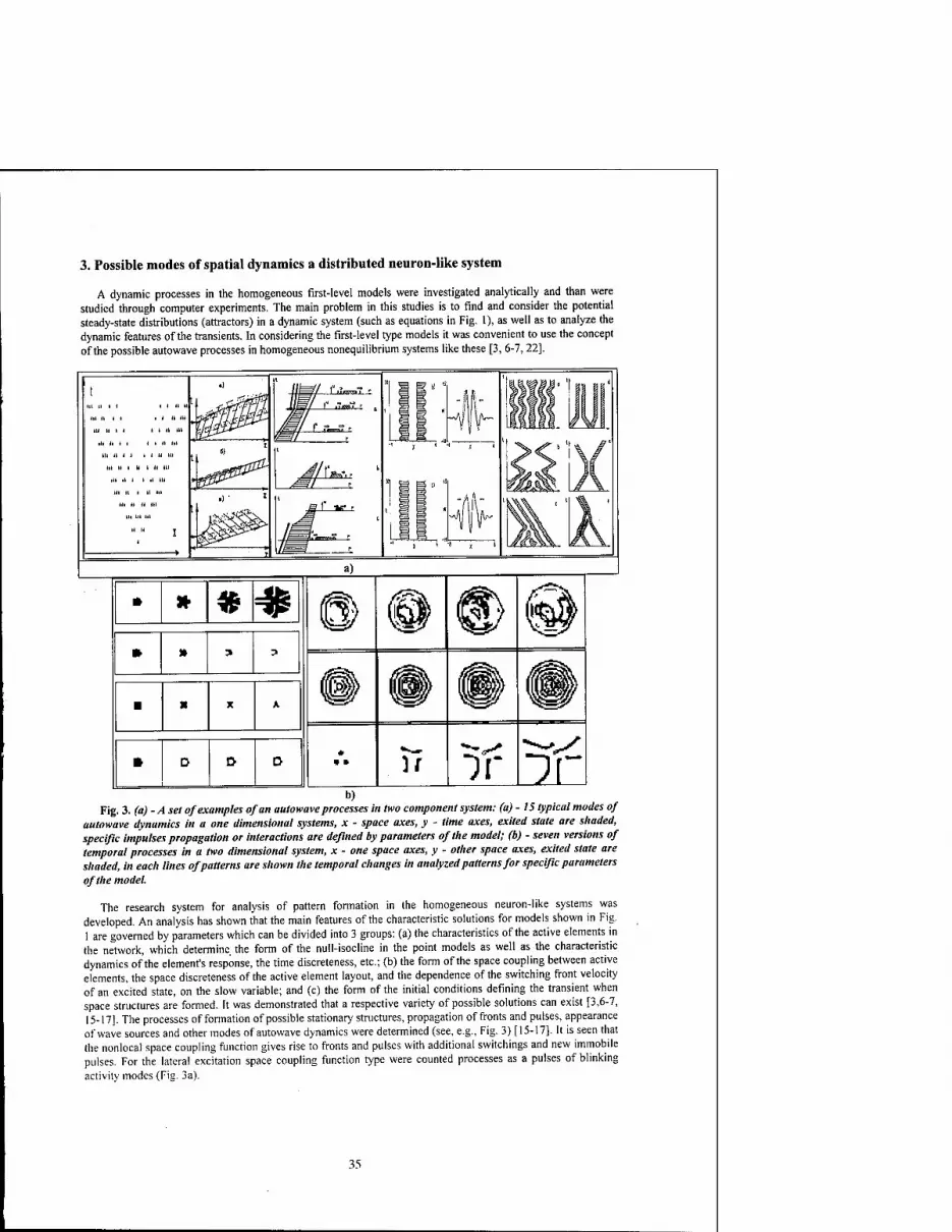
3. Possible modes of spatial dynamics a distributed neuron-like system

A dynamic processes in the homogeneous first-level models were investigated analytically and than were studied through computer experiments. The main problem in this studies is to find and consider the potential steady-state distributions (attractors) in a dynamic system (such as equations in Fig. 1), as well as to analyze the dynamic features of the transients. In considering the first-level type models it was convenient to use the concept of the possible autowave processes in homogeneous nonequilibrium systems like these [3, 6-7, 22].

■ X X A.

H If Di **s

b) Fig. 3. (a) - A set of examples of an autowave processes in two component system: (a) - 15 typical modes of

autowave dynamics in a one dimensional systems, x - space axes, y - time axes, exited state are shaded, specific impulses propagation or interactions are defined by parameters of the model; (b) - seven versions of temporal processes in a two dimensional system, x - one space axes, y - other space axes, exited state are shaded, in each lines of patterns are shown the temporal changes in analyzed patterns for specific parameters of the model.

The research system for analysis of pattern formation in the homogeneous neuron-like systems was developed. An analysis has shown that the main features of the characteristic solutions for models shown in Fig. 1 are governed by parameters which can be divided into 3 groups: (a) the characteristics of the active elements in the network, which determine the form of the null-isocline in the point models as well as the characteristic dynamics of the element's response, the time discreteness, etc.; (b) the form of the space coupling between active elements, the space discreteness of the active element layout, and the dependence of the switching front velocity of an excited state, on the slow variable; and (c) the form of the initial conditions defining the transient when space structures are formed. It was demonstrated that a respective variety of possible solutions can exist [3,6-7, 15-17]. The processes of formation of possible stationary structures, propagation of fronts and pulses, appearance of wave sources and other modes of autowave dynamics were determined (see, e.g., Fig. 3) [15-17]. It is seen that the nonlocal space coupling function gives rise to fronts and pulses with additional switchings and new immobile pulses. For the lateral excitation space coupling function type were counted processes as a pulses of blinking activity modes (Fig. 3a).

35

In a two-dimensional system, the conditions for existence of a number of new regimes were specified by analysis of stability in the propagation of a plane excitation front. The parameter regions corresponding to the different modes of propagation of a stable and unstable fronts are shown in (Fig. 3b).

The goal of a subsequent investigation is to find a more complete tree of possible solutions both in a one- dimensional and two-dimensional systems.

The obtained solutions, as a one of application, were used to interpret the dynamics of propagating depression waves in the cerebral cortex, describe the normal perception and violations in the transformation of sensor signals in physiological experiments, estimate the parameters of autowave processes in the cardiac muscle, and compare model calculations of calcium ejection autowaves in muscular cells with experimental observations.

In the other case of application, analysis of the possible solutions in homogeneous models has made it possible to find the conditions under which the initial image can be transformed into sets of simplified images needed for calculation of the video image features. There was an imitation of the following processes of parallel processing of the input signal: the contouring and skeletonization of the video images; the extraction of lines of a definite direction or objects of a definite dimension; the determination of the regions of prescribed textures and boundaries between textures, the localization of the points of intersection of lines; the joining of line segments which are parallel to the similar lines in the immediate vicinity; the "autowave" calculation of characteristic space parameters in a fragment, and some other operations (see, e.g., Fig. 4) [15-17, 22-24].

ifcy)

Fig. 4. Scheme of paths of input image transformations into a calculated "code" description of a studied image fragment.

We implemented these algorithms on the base of one - and two- components neuron-like models. All these algorithms are represent a parallel algorithm class of data processing. At present, it is possible to encode an arbitrary image fragment with various assigned objects from the input image. Hardware implementation of neuron-like architecture for such algorithms of features extraction will help drastically reduce the time of complex image processing.

4. Current versions of making a decision system.

Various algorithms of image transformation in the classical pattern recognition theory extract sets of most characteristic "code" features of the object being identified (see, e.g., [9-10]). In the theory of parallel calculations in neuron-like media, such algorithms are represented by the architecture of systems with a "coarse- grain" structure as in the Fig. 2 [8, 15-17]. Each subsystem of such a system performs its assigned operation and is situated in a certain "branch" of the data transformation path (succession of algorithms). In such a scheme, it is important to choose the minimum possible universal architecture for implementation of automatic-tuning algorithms in the identification of any assigned object on an arbitrary complex image.

A research system for analyzing adaptive algorithms was also developed in the AWP team working with 1AP RAS. The found adequate modes of recognition were used for the development of an "Oncomorfologist" system to distinguish between normal and pathological cells during medical diagnostics of oncological diseases, the system of biometry of hand, the system for automated identification of a person by his hand and fingerprint, etc.

In particular, the tuning algorithm connected with the choice of an optimal recognition threshold for each class (user) from all the data registered in the archive database was checked by testing statistical characteristics of accuracy of the "Hand-Identification System" (HIS-1). This allowed the recognition accuracy to be increased by several times. We showed the possibility of description of adaptive image-identification facilities as multilevel neuron-like elements. Variants of the dynamics of the response of such nonlinear systems with many interconnected components were considered.

The formation of "algorithmic language" for adequate description of dynamic processes in hierarchic neural- like systems and the use of the data for constructing such intellectual users-computer interfaces is one of the key elaborations of the AWP team investigation.

Using the model of adaptive image recognition (as shown in Fig. 2), a data structurization scheme for neuron- like systems were developed. This informational data base include a set of models, basic characteristics for qualitative analysis of solutions, a set of solutions corresponding to AWP and similar structures, a set of experimental examples and their interpretation, and variants of technical applications. This scheme permits one to

36

combine from a unified basis the various data on distributed biological systems and find analogues in their dynamics. The scheme is used as a method for presentation of materials in teaching students and in discussions with other specialists in autowave dynamics.

5. Conclusion

Temporal variations of spatial activity structures in distributed biological media are encountered at all hierarchic levels, including molecular, membrane, cellular, population and other levels, and almost everywhere such "nonlinear modes" of active states are connected with the corresponding variants of operating modes of a biological object. It appears that the dynamics of many biological and corresponded them artificial systems is described by a special set of basic mathematical models referred to the class of models of homogeneous neuron- like systems. It can be stated that the main features in the behavior of living systems and their simplest analogues in physical or chemical systems are determined primarily by the laws of interaction dynamics of spatial activity structures in neuron-like systems. Hence, the data on the dynamics of self-organized activity structures (referred to as autowave processes, dynamical structures, etc.) form a "language" to describe operating modes in biological tissues. For this area of nonlinear dynamics study were also formulated the concept, known as the Cellular Neural ANonlinear Network (CNN).

In this communication, the most typical basic models of neuron-like media which describe both homogeneous systems (level 1) and hierarchic levels of recognition of complex activity patterns (neuron-like systems of levels 2 and 3) are considered.

The results of studies of the possible dynamics of spatial structures are presented. Examples of the dynamics of parallel transformation modes of a complex pattern of sensor images are demonstrated.

The obtained solutions were used to interpret the dynamics of propagating autowaves in some biological tissues. The adaptive modes for a decision-making system were considered. Examples of artificial recognition automata for extraction of an initially assigned video image with a minimum possible error were created.

6. References

1. Wilson H.R., Cowan J.D. "A Mathematical Theory of the Functional Dynamics of cortical and Thalamic Neuron Tissue", Kibemetic , Vol. 13, pp.55-80, 1973.

2. Sbitnev V.l. "Spike transfer in the statistical neuron ensembles. II. Neuron-non-linear source of spikes", Biophysics, Vol. 21, pp. 1072-1076, 1983.

3. Kudryashov A.V., Yakhno V.G. "Propagation of domains of rised pulse activity in a neuron assembly". "Dynamics of Biological Systems" (Inter-University collection, Gorky State University), No. 2, pp.45-59, 1978, (in Russian)

4. Frolov A.A., Murav'ev I.P. "Neural models of associative memory", M., "Nauka", 1987, (in Russian) 5. Sokolov E.N., Vaitkyavichus G.G. "Neurointelligence: from neuron to neurocomputors", M., "Nauka",

1989, (in Russian) 6. Masterov A.V., Rabinovich M.I., Tolkov V.N., Yakhno V.G. "Investigation of the autowave-autostructure

interaction regimes in neural media", Collection of Institute of applied physics "Collective dynamics of excitations and structure formation in biological tissues" , Gorky, pp.89-104, 1988.

7. Yakhno V.G. "Basic models of hierarchy neuron-like systems and ways to analyse some of their complex reactions", Optical Memory&Neural Network, v.4, No2, ppl41-155, 1995.

8. Arbib M.A. "Schemes and neural networks for sixth generation computing", Journal of Parallel and Distributed Computing, Vol. 6. No 2, pp.185 -216, 1989.

9. Braverman E. M., Muchnik I. B. "Structural methods of empirical data processing", M., "Nauka", GRAML, 1983 (in Russian).

10. Duda R., Khurt P. "Pattern recognition and scene analysis", M., MIR, 1976, (in Russian) 11. Fukushima K. "Neural network model of selective attention in visual pattern recognition and associative

recall", Appliede Optics, v.26, N23, pp.4985-4992, 1983; Neural network for visual pattern recognition. Computer, pp. 65-67, 1988.

12. Fukushima K. "Cognitron: a self-organizing maltilayered neural natwork model", NHK Technical Monograph, N30, 1981. NHK Technical Labs.Tokyo. "Neocognitron: a new algorithm for pattern recognition tolerantof deformation and shifts in position", Pattern Recognition,V1.15.P.455-169, 1982.

13. Zverev V.A. "Physical Foundation of image formation by wave fields", IAP RAS, 252p, 1998. 14. Telnykh A.A., Yakhno V.G. "Neuron-like models of the second and third levels - adaptive recognition

system", Proceeding of XII International conference on Neurocybernetics "Neurocybernetics Problems", pp. 164- 168, 1999.

37

15. Belliustin N.S., Kuznetsov S.O., Nuidel I.V., Yakhno V.G. "Neural Networks with Close Nonlocal Coupling for Analysing Composite Images", Neurocomputing, Vol..3, pp. 231-246, 1991.

16. Yakhno V.G., Nuidel I.V. "Modeling of sensory information transformations". " Neurocomputer as the basis of thinking computers", M. Nauka.l993.P.207- 223.

17. Yakhno V.G., Belliustin N.S., Krasilnikova I,G., Kuznetsov S. O., Nuidel I.V., Panfilov A.I., Perminov A.O., Shadrin A.V., Shevyrev A.A. "Research Decision-making System Operating with Composite Image Fragments Using Neuron-like Algorithms ", Radiophysics, Vol.37, N8, pp.961-986, 1994.

18. L.O.Chua and L.Yang, "Cellular Neural Networks: Theory. Applications", IEEE Trans. On Circuit and Systems, (CAS), Vol. 35. Pp.1257-1290,1988.

19. L. 0. Chua, T. Roska, "The CNN Paradigm", IEEE Transactions on Circuits and Systems I. Vol.40, No.3, 1993, pp.147-156.

20. Cs. Rekeczky, T. Roska, and A. Ushida, "CNN-based Difference-controlled Adaptive Nonlinear Image Filters", International Journal of Circuit Theory and Applications, Vol. 26, pp. 375-423, July-August, 1998.

21. Cs. Rekeczky and L. O. Chua, "Computing with Front Propagation: Active Contour and Skeleton Models in Continuous-time CNN", Journal of VLSI Signal Processing Systems, Vol. 23, No. 2/3, pp. 373-402, November-December 1999.

22. Cs. Rekeczky, "Active Contour and Skeleton Models in Continuous-time CNN", to be presented in Special Session of the 14th IEEE European Conference on Circuit Theory and Design ECCTD'99 in Stresa, August 1999.

23. Vasiliev V.A, Romanovskii Y.M, Chernavskii D.C., Yakhno V.G. "Autowave Processes in Kinetic Systems. Spatial and Temporal Self-organization in Physics, Chemistry, Biology, and Medicine". VEB Deutscher Verlag der Wissenschaft, 1987, GDR

24. Nuidel I.V., Kuznetsov S.O. "Using of Neural Networks for Image Processing", Radiophysics, Vol.37, N 8, pp.1053-1061, 1994.

25. Kuznetsov S.O., Nuidel I.V., Panfilov A.I., Yakhno V.G. "Image preprocessing by neuron-like algorithms", The Proc. SPIE "Optical Information Science and Technology" in Optical Memory and Neural Networks, Andrei L.Micaelian, Editor, Proceedings of SPIE Vol.3402, pp. 479-485, 1998.

38

2000 6TH IEEE International Workshop on Cellular Neural Networks and Their Applications Proceedings

Straightforward Design of Robust Cellular Neural Networks for Image Processing

David Monnin1,', Lionel Merlat', Axel Köneke1, Jeanny Herault?

1 French-German Research Institute of Saint-Louis PO Box 34, 68301 Saint-Louis Cedex, France

monnin@isl.tm.fr, monnin@ece.fr

2 LIS Laboratory, INPG, 46, avenue Viallet, 38031 Grenoble Cedex, France

ABSTRACT: The analytical design of Cellular Neural Networks (CNNs) templates for image processing often goes through the resolution of pixel level analytical rule-based task descriptions in- volving ideal CNN models. Due to non-ideal analog implementations of CNNs, recent issues have ad- dressed the template robustness in order to achieve fault-tolerant processing. However, besides their efficiency and usefulness for the definition of coupled operators, rule-based approaches can make CNN templates design appear to be an intricate art reserved for initiated CNNs specialists rather than for image processing scientists. An alternative straightforward analytical design method for uncoupled CNNs, which is until now the only unified approach to the design of both gray and binary output op- erators, has already been presented, and is now extended to the design of robust binary operators.

1. Introduction

Cellular Neural Networks (CNNs) [1] are lattices of analog locally connected cells conceived for an implementation in VLSI technology and perfectly suitable for analog image processing. The operation of a cell (i, j) is described by the following dimensionless equations:

—i£- = -xij+A®yij+B®uiJ + I (1) dt ' '

^■(^(KH-hH) (2)

where ® denotes a two-dimensional discrete spatial convolution such that A ® ytj = Ejy6j\r(i,j)4fc,i,!'>-t,;-i for k and I in the neighborhood N(i, j) of cell (i, f), which is generally re- stricted to the 8-connected cells. A and B are the so-called feedback and feedforward weighting matri- ces, and / is the cell bias. u{j, xitj and yt■ are the input, internal state and output of a cell, respec- tively. The same set of parameters A, B and J, also called cloning template, is repeated periodically for each cell over the whole network, which implies a reduced set of at most 19 control parameters, but nevertheless a large number of possible processing operations.

Efficient methods for the analytical design of robust CNN binary image processing operators can be found in the literature [2], but none of them allows the design of gray level operators as well. On the other hand, the final results they provide must often be decomposed to achieve fault-tolerant process- ing on analog hardware [3]. An alternative design method for uncoupled CNNs was formulated from the principle of convolution masks used in a large number of well-known image processing algo- rithms [4]. This method opens the application field of analytically designed CNNs to numerous tradi- tional operators for binary and gray level image processing, among which all linear convolution filters as well as Boolean and morphological operators can be found. After a short overview of this approach, the issue of binary output operators will be discussed in detail. Finally, thanks to the formalism chosen in the method, the robustness of binary operators will be effortlessly tackled.

2. Analytical Design of Gray Level and Binary Operators

Whether it is called convolution mask or structuring element, depending on whether the processing intended is a convolution filter or a morphological operator, the feedforward matrix B involved in a CNN image processing operator is here custom-defined or modeled on the definition of a traditional digital image processing filter, while parameters o and I are determined from the design method out- lined in the next subsections.

As stated in [4], two primary categories of CNN image processing operators can be defined de- pending on the value of the feedback parameter a: those providing a gray level output when o < 1, and and those providing a binary output when o > 1.

0-7803-6344-2/00/S10.00 ©2000 IEEE 39

2.1 Gray level output image processing operators

A CNN can perform a linear convolution filtering using feedforward matrix B as a convolution mask, and can even simultaneously rescale the original range [m, n] of the input image to a desired range [M, N\. This is possible by determining the parameters a and /as follows:

° = 1-|W-¥^'and/ = iVH~-" (3a-b)

Furthermore, a "reverse video" effect can be obtained by simply reversing the sign of B and using a new original range which is symmetrical to the old one with respect to the origin and yields a new cur- rent constant /' = 7+n-t-m.

2.2 Binary output image processing operators

In the case of binary output image processing operators, the convolution operation mentioned be- fore remains and the role of the feedforward matrix B is maintained, but the result of the processing is now thresholded. Then the determination of parameters a and / has to deal with the value of one or two thresholds, as will be outlined in the following subsections where several variants of the same principle are presented.

Single threshold processing. The purpose of the simplest variant of the method is to threshold the result of a linear convolution filter at a desired threshold Th. Parameters a and / are then such that:

o > 1, and / = (1 - o).x(0) - Th , (4a-b)

where the initial state x(0) e [-1, +1] is the same for all cells of the network. In addition, an inver- sion effect is obtained by reversing the sign of B and Th.

Two thresholds processing. The aim of this second variant of the method is to threshold the result of a linear convolution filter with two different thresholds assigned to particular cells according to their input state. In this case parameters a and / are expressed as:

. Th'-Th* , . i-(0)-TA+-x+(u)-Tft- /c _ o = 1 + , and / = —^ K—t , (5a-bl

x*(0)-x-(0) x+{0)-x-(0) K '

where Th' applies to cells with an initial state z(0) e [-1, +1], and Th+ to cells with an initial state i+(0) e [-1, +1], such that x'(0) < x+(0) and Th' > Th+.

Single threshold processing and Boolean operators. This is an adaptation of the previous method which allows to combine a binary initial state with the result of a thresholded convolution fil- ter.

"OR" Boolean operators are obtained when:

Th' = "threshold value" and T/i*<-llfll, (6a-b)

"AND" Boolean operators are obtained when:

TK £ IIBII, and Th+ = "threshold value" (7a-b)

Once again, an inversion effect can be obtained by simply reversing the sign of B and of the thresh- old value.

3. Straightforward Design of Binary Output Operators

Instead of going through the resolution of pixel level analytical rule-based task descriptions, the de- sign of binary operators can be directly derived from the appropriate convolution masks B and thresh- olds Th, using the method presented in the previous section. The determination of B and Th for binary operators is clarified here in the light of Boolean algebra and mathematical morphology.

40

3.1 The Boolean approach

A CNN binary output operator can be regarded as a Boolean operator combining, in a Boolean re- lation, inputs of cells within the local interaction neighborhood. Assuming that CNN cell values 1 and -1 respectively mean TRUE and FALSE, every Boolean function can be implemented using one or sev- eral cloning templates. As long as they remain linearly separable, many Boolean expressions can be performed by a single CNN binary output operator. The determination of the feedforward matrix B and the threshold Th for some basic Boolean operations is presented here.

Boolean product. A CNN cell is here intended to implement a Boolean product of variables chosen among its own input «„ „ and the inputs uK, of cells within its neighborhood N(k, I). The cell output y can therefore be expressed as:

W= II"*.'' EX" ^ (i,!)eW*(i,l> (k,l)eN-(k,l)

where N*(k,l) and N~(k,l) are non-overlapping subsets of the cell neighborhood N(k,l).

In other words, the cell output y is considered to be TRUE, i.e. is equal to 1, if and only if all in- puts of cells within the local interaction neighborhood match exactly the given logical expression. Since CNNs implement thresholded convolution products, in order to determine if a set of inputs matches a given expression, we define a convolution mask held in feedforward matrix B, for which the convolu- tion product reaches a maximum when the logical expression is satisfied. Consequently, B coefficients bt | must in a way reflect the logical expression and are chosen such that:

( b, to match ukl

bkl=\ — b, to match 5ti( (9)

[ 0, for " don't care"

Finally, in order to select only maximum values of the convolution product and given that convolu- tion products take only discrete values with binary inputs, the threshold Th is simply adjusted be- tween this maximum and the closest lower value, which yields:

The X ki-"t,i|-2-6, Xk, •"*,■ (t,l)6,v(fc,l) (M)eiW*,0

.n6]|B||1-2.»,|B|1[ (10)

Boolean sum. If a CNN cell implements a Boolean sum, its output y is given by the following expres- sion:

V= IX'+ IX" (11) (M)eJV*(i,l) (H,l)e«-(*,n

where N*(k,l) and N'(k,l) are non-overlapping subsets of the cell neighborhood N(k,l).

In plain language, the cell output y is considered to be TRUE, or equal to 1, if and only if at least one among the inputs of cells within the local interaction neighborhood matches a variable of the logi- cal expression (11). Following the same approach as previously, B is chosen according to (9), but the values of the convolution product which satisfy the logical expression are now those greater than or equal to the convolution product obtained when only one coefficient of B matches an input value. Hence, the threshold Th is chosen between this value and the closest lower value, which leads to:

The - X ki'ut,i|'- Xki'^'r2'6

He»(l,l) (M)eJV(*,l)

.77,e]-||4,-|B||1+2-i,[ (12)

Boolean n-matching operation. The Boolean sum of all possible n-variables Boolean products can be described as a kind of Boolean sum for which at least n matching variables are required for the ex- pression to be regarded as TRUE. For simplicity's sake, the cell output y is then expressed as:

V= XUM + IX" (13)

(fc,!)eJV*(M) (t,l)eJV-(l:,l)

where N*(k,l) and N'(k,l) are non-overlapping subsets of the cell neighborhood N(k,l).

41

The cell output y is now considered to be TRUE, or equal to 1, if and only if at least n among the inputs of cells within the local interaction neighborhood match a variable of the logical expression (13). B is again chosen according to (9), and the values of the convolution product which satisfy the logical expression are those greater than or equal to the convolution product obtained when at least n coeffi- cients of B match an input value. Once more, the threshold Th is chosen between this value and the closest lower value, which gives:

The •UM+2(B-!)•&, (k,l)eN(k,l)

- Sk' 'UM| + 2n'b

(M)EJV(*,1)

»»E]- 14 + 2(n -1) ■ b- j^ +2nb[

(14)

Boolean n-matching operation in which a Boolean product is involved. An n-matching op- eration involving a Boolean product can also be performed in a single CNN operation. The cell output y is then defined as:

y= X"*.'+ Xu*.' +

Jt,l)e.V'(t,Q (t,l)<;JVf (i, /) (15)

where N*(k,l) and N~(k,l) are non-overlapping subsets of the cell neighborhood N(k,l).

This operation combines a Boolean product and an n-matching operation respectively described by their B, and Bs feedforward matrices, both designed in the way presented previously. The overall feedforward matrix B and the choice of a suitable threshold Th are then given by:

B =

The

lä-^+B,,

-M.Nli+(2n_1).|ßiii_2ii_ML.Nli+(2n_1).iSilli

(16a)

(16b)

Boolean product of a Boolean product and a Boolean n-matching operation. A Boolean product involving a Boolean product and a Boolean n-matching operation can as well be performed in a single CNN operation. The cell output y is then given by:

y= nuv Wut,i (t,/)eJVj(t,l) (k,i)eN;(k,ri (*,!)« W|*(*,l) (M)EArf(*,l)

(17)

where N+(k,l) and N~(k,l) are non-overlapping subsets of the cell neighborhood N(k,l).

This operation combines an n-matching operation and a Boolean product respectively described by their B, and B, feedforward matrices, both designed in the same way as before. The overall feedfor- ward matrix B and the choice of a suitable threshold Th are then given by:

IN b

■ + l-n ■B..+B, (18a)

The b !"" ■ lß2 II - lßi II,+2("-1)-''.

m •+ l-n Pi , +2nb (18b)

Further Boolean operations. Other Boolean operations can also be performed in single CNN opera- tions. This kind of operation, like for example a Boolean product including a Boolean sum, itself in- cluding a Boolean product, can be derived from the previous approach. However, complex Boolean functions combined in single CNN operations often lead to poorly robust operators which ought to re- main simple in order to achieve fault-tolerant operations [3]. Actually, simple Boolean functions ought to be linked into a CNN processing scheme successively combining, through Boolean operators, the result of an operation with the result of a previous one stored in the CNN initial state [4, 5].

42

3.2 The morphological approach

In the field of mathematical morphology, numerous very interesting binary image processing opera- tors were defined in terms of pixel set operations [6]. CNNs can easily implement all binary morpho- logical operators. In this case, the feedforward matrix B plays the role of a so-called structuring ele- ment, where b positive coefficients stand for black pixels, -b for white ones, and 0 for "don't care". The B "structuring element" acts on the input image U, and moreover, the operation result can be coupled with a CNN binary initial state through union or intersection operators.

Although they are based on set operations, whereas Boolean operators are based on algebraic op- erations, and convolution operators come under arithmetic operations, morphological operators can be easily transposed from the set theory to the Boolean algebra for which the transposition to the arithm- etic of thresholds and convolution masks has just been explained before. The two main morphological operators, from which all other operators are composed using union, intersection or complement opera- tions, are erosion and dilation. Those operators as well as their equivalence to Boolean operators are briefly introduced in the following subsections.

Morphological erosion. The erosion of a binary image U by an avcentered structuring element (B)„ is the set of pixels x such that (B)x completely matches the pixels of U. This can be expressed as:

UQB = {X\(B\QU}, (19)

This definition is a kind of translation of the Boolean product definition of equation (8) into the set theory language. Hence, apart from the theoretical point of view, a morphological erosion can be re- garded as a Boolean product and implemented in the same way.

Morphological dilation. The dilation of a binary image U by an x-centered structuring element (B)„ is the set of pixels x such that the reflected structuring element has at least one pixel matching a pixel of U. An expression of dilation is given by:

tf©B = fr|[(ß),ni/]*0} (20)

On thinking it over, this definition also has an equivalent in the Boolean algebra. Actually, beyond theoretical considerations, a morphological dilation can be related to a Boolean sum (11) and designed identically.

4. Robustness Optimization of Binary Output Operators

Due to intrinsic noise, time and temperature drifts of components, as well as fabrication defects, analog VLSI implementations necessarily conduct to non-ideal CNN chips, which CNN software has to deal with. The ability of a CNN image processing operator to still produce the right output even with slightly deteriorated parameters is called robustness.

Actually, robustness considerations especially apply to binary input operators for which the convo- lution product B ® ui7 describes a discrete set of possible values. As explained in the previous section, binary operators involve a decision border which can be materialized in the form of a threshold. CNN parameters deviations make the convolution products B ® u^ deviate from their theoretical values, but do not cause any faulty operations as long as the decision border is not violated. In order to opti- mize binary operators for robustness, it is then necessary to move the thresholds away from any theo- retical value of B ® ui7-, which implies to choose the thresholds in the middle of the intervals defined in the previous section, i.e. at a confidence distance b of any theoretical value of a convolution prod- uct. This confidence distance b must also be respected for operators combining, through a Boolean op- eration, a binary initial state with the result of a binary operation. This requires thresholds in (6b) and (7b) to be respectively chosen as:

Tti = -IIBII, -6, and TK = IIBII, +b (21a-b)

Following a similar approach to the one in [2], the relative and absolute measures of robustness can now be expressed as:

>■ b and p = —, (22a-b)

14+14+IT N' where Nis the total number of non-zero parameters involved in A, B, and 7.

43

Scaling up a cloning template by increasing parameter b improves both the relative and absolute robustness. Furthermore, by making assumptions on the upper bounds of a CNN dynamics, it is possi- ble to determine the largest possible value of 6 and thus to derive the optimally robust template with regard to these assumptions [2j.

5. Conclusion

An alternative straightforward analytical design method for uncoupled CNNs, which offers an original unified approach to the design of both gray and binary output operators, has been presented here and extended to the design of robust binary operators. Based on the use of convolution masks, this approach additionally allows the robust implementation of all Boolean and morphological binary operators.

First introduced for uncoupled CNNs, this method is being successfully adapted to some specific coupled tasks, and is expected to be generalized for application to coupled CNNs. In other respects, it is interesting to notice that, as different cloning templates can lead to the same operation, the space described by CNN parameters is wider than that of operators. This suggests that heuristics, suitable for downsizing the CNN parameters space and making it fit that of operators better, would certainly drastically improve stochastic optimization algorithms like genetic algorithms or simulated annealing. Since their respective functional role is not clearly established, it is difficult to make any assumption on the CNN parameters to judiciously reduce the space they describe. On the other hand, convolution masks or thresholds have a specific function which can be used to bring the CNN parameters space closer to that of the operators. For example, the use of normalized convolution masks does not de- crease the number of realizable operators, but significantly reduces the functional redundancy of the CNN parameters space. Hence, in addition to the original contribution of the method to the analytical design of CNN operators, the approach tackled here would very likely be profitable for stochastic op- timization algorithms.

6. References

[1] L. O. Chua and Yang: "Cellular Neural Networks Theory", IEEE T-CAS, Vol. 35, pp. 1257-1272, 1988.

[2] M. Hänggi and G. S. Moschytz: "An Exact and Direct Analytical Method for the Design of Opti- mally Robust CNN Templates", IEEE T-CAS I, Vol. 46, pp. 304-311, 1999.

[3] P. Földesy, L. K£k , Ä. Zarändy, T. Roska, and G. Bärtfai: "Fault Tolerant Analogic CNN Tem- plates and Algorithms-Part I: The Binary Output Case", IEEE T-CAS I, Vol. 46, pp. 312-322, 1999.

[4] D. Monnin, L. Merlat, A. Köneke and J. Herault: "Design of Cellular Neural Networks for Binary and Gray Level Image Processing", Proc. of ICANN'98, pp. 743-748, Skövde, Sweden, 1998.

[5] D. Monnin, L. Merlat, A. Köneke and J. Herault: "An Investigation into Cellular Neural Networks Internal Dynamics Applied to Image Processing", Proc. of IWANN'99, Vol. II, pp. 432-441, Ali- cante, Spain, 1999.

[6] J. Serra: "Image Analysis and Mathematical Morphology", Academic Press, New York, 1982.

44

2000 6™ IEEE International Workshop on Cellular Neural Networks and Their Applications Proceedings

Modelling of Extraction of Image Fragments in the Forms of Crosses and Rhombuses

in the Simulated Receptive Fields

Nuidell.V., YakhnoV.G.

603600, Nizhny Novgorod, Ul'yanov str, 46, Institute of Applied Physics RAS, e-mail: nuidel@awp.appl.sci-nnov.ru

ABSTRACT: Understanding of possible regimes of animal reactions is based on consideration of possible variants of spatial-temporal dynamic processes of feature extraction from the input stimulus. Detection of crosses and rhombuses, that have been registered in the neurophysiologic experiments, is simulated. The model of one of the functional regimes registered at the experiments of animals has been proposed.

1. Introduction

Understanding of possible regimes of animal reactions is based on consideration of possible variants of dynamic processes of feature extraction from the input stimulus [1-5].

At present the study and computer simulation of the possible response of primate to receptor signals have very important applications [6]. New interesting data on the ability of individual visual neurons and ensembles of neurons to process and extract features in complex visual signals have recently been obtained.

In recent decades, there have been intense experimental studies extracting image features of different complexity, including the orientation of line segments [1-4], features of the second order, such as intersection and nets of line branching (crosses, corners, and y-type figures) [2,5]; features of higher orders such as face [4], and spatio-frequent tuning of visual cortex neurons. Thus, there is progress in filling the gap between the orientation detectors described in the primary visual cortex and the detectors of higher orders, for example face, found in the lower-temporal cortex.

2. Neurophysiological data

Experimental studies of the selective and invariant sensitivity of neurons in cat's visual primary cortex to features of the second order, such as line crosses and nodes of line branching were performed [2,3,4]. The receptive field of these neurons were investigated by the method of point by point mapping for the estimation of structures of input couplings of neuron [2,3,5]. The dynamics of tuning of the receptive field of these neurons was also investigated by the method of temporal slicing to discover the role of temporal dispersion and temporal organisation of the input signal in the extraction of the image features by the cell.

The role in the recognition of such features as segment of lines, corners and more complex nodes of counter branches was determined through Psychophysical investigation of man recognition of complete and particularly masked or uncompleted images.

For the first time in the primary visual cortex the scanning detectors were found. Their tuning are changed successfully during forming the response of stimulus. The existing of such neurons proposes the possibility both place and spatio-temporal coding of orientation information at this level of the visual system [2,3]. The sensitivity to line intersection, crosses, corners of 40% neurons was founded and investigated experimentally. At present the gap in the understanding of sequence of the operations of extraction from the image the higher order features are filled.

At present, it is very interesting to examine which properties of the actual neural network provide the detection of geometric figures. The task of this paper is to simulate the possible coupling structure, which ensures these properties, by using neural network model.

3. Overview of models

On the basis of physiological data, models of neuron ensembles of visual cortex as a system of phase-locked coupled oscillators were proposed to extract image features are developed [7]. However, such models extract only a limited set of features from the initial model image in the form of strokes of different orientations, such as contour, boundaries between textures, image segmentation, etc. These models do not give unreasonably high saliences to the short segments of contours smoothly are attached to long smooth contours.

0-7803-6344-2/00/$10.O0 ©2000 IEEE 45

The family of 2D filters was introduced by Daugmen [8] as a model for the structure of simple-cell receptive- field profiles, and they are termed 2D Gabor functions. Experimental work by Jones and Palmer [9] confirmed that this family of functions corresponds well the receptive field profiles of a simple cell in the primary visual cortex of cats.

Linear filtration by Gabor functions is used to extract image features, encode images by expansion coefficients with respect to the nonorthogonal basis of Gabor functions [8].

A model for the formation of spatio-temporal receptive fields of simple cells in the visual cortex is proposed on the basis of the convergence of four types of input of a cortical cell from lagged and non-lagged ON and OFF inputs [10]. One limitation of this model is that the input are described by the product of linear spatial and temporal response functions. Another limitation is that the model does not include intracortical interactions.

We investigate integro-differential equations that are basic models of homogeneous distributed neuron-like media [11-18,22]. They were obtained as a balance equations for spikes in the fibers of exciting and inhibitory neuron networks [11,12,23,24],

4. Model of a homogeneous distributed neuron-like system

Two-dimensional neuron receptive fields are actual examples of biological non-equilibrium media. The model of this medium describes the reaction of a neural network that transforms input images from their receptive fields. The form of the receptive field corresponds to weights of coupling function in the layer. Couples are assigned in the local area inside the layer. The functional mode of coupled neuron-like elements for feature extraction is simulated is simulated during the formation of the response for grey-tone image. A parallel-series transformation of the initial image was implemented. Models (l)-(4) describe a parallel image transformation process for matrices with a programmed structure of couples [14,15,17].

Tuaya = -U+F -T + a Jo„(|-r)-U^,()^ + üex(r-,()

0,Z<0

F[Z]=Z,Z e[0,255]

255, Z> 255

<t>(r -n))= N(\ -b(r -?0)2)exp- a(f -?Q)

2.

r =(x,y)

(1),

(2),

(3),

»U1=»"jO-'u/T ) + -F '•J '•■/ / Tu r„

k = M,l=D

-T+a Z %<*,;+/+"a

k=-M,l=-D

(4)

Here, u(r,t) = u(x,y,t) - describes the excitation in the patterns at the two-dimensional distributed neuron-

like system (image byte per point). xu - is the relaxation time for the initial condition, T is the threshold of

active elements on the general external signal from the coupled field. <S>u(f) is coupling function of the lateral inhibition type with positive centre and negative surround, a - is the norm constant for coupling function. Non- linear function F[Z] is written in piece-wise linear presentation (2) and characterises the generation and evolution processes. A difference scheme of the distributed model equation (1) in the type (4) was also implemented. Here, tu is the temporal digitisation, O^ / is a matrix in the convolution procedure [12-18].

A similar model, known as the Cellular Neural/Nonlinear Network (CNN), was examined in [19-22]. It is also possible to use a model that is more complicated than that described by (l)-(4) where two or three

layers are used and some possible types of their interactions are introduced [13-15]. First, pattern formation processes in the model were investigated analytically and than were studied through

computer experiments. The research system for analysis of pattern formation in the OS Windows, DOS was developed. The processes of formation of possible stationary structures, propagation of fronts and pulses, appearance of wave sources and other modes of pattern formation were determined [13-18].

In a substance, data processing in the homogeneous distributed neuron-like systems is the process by which a set of possible autowave processes is chosen and simplified patterns (preparations) from the input image are formed. These patterns can be interpreted as an extraction of simple preparations from the input image. For

46

example, from the immobile grey-tone image the counter or lines of the determined directions and so on were considered from middle 80-th years in the team of autowave processes (AWP team) working in IAP RAS [12- 18]. The analogous examination independently were developed on the base of CNN-paradigm in papers [19-22].

5. Simulation

Two coupling functions with orthogonal directions of änisotropy are summed for coupling function forming of extraction of cross and rhombus fragments from the input image.

By the program NET.EXE all computations have been carried out. Sizes of the layer are from 0 to 512

elements pixels. <!>£/ is the element of the coupling function <&(!; - f). Sizes of convolution function is equal or

less than the layer size. (2M+1)*(2D+1) - the size of the coupling function (matrix in the convolution procedure). 0(-M)(-D) ... 0(M)(-D) 0(-M)(D) ... 0(M)(D) 0kl is changed within the range : -256< 0kl <256, Qy = 255 • <b(x, y)-M <k<M-D<l<D

(2M + l)*(2D + \) 11 (2M + l)*(2D + \) 15 0 0 0 0-3-8-30000 000-1-2 00000-2-1000 0 0 0 0 -8-18 -8 0 0 0 0

0 0 0 0-16-14-16 0 0 0 0 0 0 0 -2-21 23-21 -2000

-3 -8-16-21-34 78-34-21-16 -8 -3 -8-18-14 23 78 80 78 23-14-18 -8 -3 -8 -16 -21 -34 78 -34 -21 -16 -8 -3

0 0 0-2-7-8-20 -2 -8-7-2000 0 0 0 0 -8-18-17-10-17-18 -80000

-1-2 0 0 -2-17-24-40-24-17 -2 0 0-2 -1 -2 -7 -8 -2 0-17-25 80-25-17 0 -2 -8 -7 -2

0 -8-18-17-17 6 104-10 104 6-17-17-18 -8 0 0-2-17 -24 -25 104 6 -24 6 104 -25 -24 -17 -2 0 0 0-10-40 80-10-24 0-24-10 80-40-10 0 0

0 0 0 -2-21 23-21 -2000 0 -2-17-24-25 104 6-24 6 104-25-24-17 -2 0 0 0 0 0-16-14-16 0 0 0 0 0 -8-18-17-17 6104-10 104 6-17-17-18 -8 0 0 0 0 0 -8-18 -8 0 0 0 0 -2 -7 -8 -2 0-17-25 80-25-17 0 -2 -8 -7 -2 0 0 0 0-3-8-30000

General sum of coefficients: -30 -1-2 0 0 -2-17-24-40-24-17 -2 0 0-2-1

0 0 0 0 -8-18-17-10-17-18 -80000

Parameters of coupling function: L-5.0. b=0.15, a=0.16, e=3, cp\ = 0,^2 = 90

0 0 0-2-7-8-20 -2 -8-7-2000 000-1-2 00000-2-1000

General sum of coefficients: -336 Parameters of coupling function :L=6.0, b=0.1.

a=0.11, e=4, <p\ =45,<p2 = 135

Table 1. Example of the coupling function for extraction of crosses and rhombuses.

Images of byte by point are used as initial conditions for the neuron-like system. The meaning u(ij) is changed within the range of integer numbers [0,255].

Forming simple binary patterns from the initial image at the one-layer neuron-like system with close non-local coupling function between elements of lateral inhibition type, are examples of non-linear filtration of the initial image.

6. Results

Successful modelling of spatio-temporal dynamics allowed us to develop algorithms for extraction image features. Only by changing parameters without model changing it is possible to obtain a lot of variants corresponding to the required transformation of input images for feature extraction. Algorithms for the formation of the simplified patterns (preparations) were developed for a one-layer two-dimensional neuron-like medium with close non-local coupling function of the lateral inhibition. A non-linear filtration was also implemented in such system. Using examples of various images, we extracted simple binary patterns, such as a contrast, counters of a certain thickness, ends of the line segments, corners, central axes of figure, objects of certain dimensions, line of certain directions, etc. [13-18]. We implemented algorithms for extraction of the desired fragments such as boundary textures, objects of certain directions or textures by using a set of one- or two-layers systems. All these algorithms belong to a parallel algorithm class of data processing. At present, it is possible to simulate responses of receptive fields on the input image fragment with various configuration such as crosses, rhombus. Some examples are shown in Fig.l, Fig.2.

47

Modelling of the spatio-temporal dynamics allowed us to develop software for extraction of image features. Obtained results were used for designing systems some recognition systems: "Oncomorfologist" for distinguishing between normal and pathological cells during medical diagnostics of oncology diseases; a system for automated identification of a person by his hand and fingerprint.

Figure 1: Extraction of cross fragments (a) and rhombus fragments from the input image of industrial objects; (b) - two types of combined textures are presented.

Figure 2: Extraction of cross fragments (a) and rhombus fragments from the initial image. On the figure 2 crosses and the input image are combined.

7. Conclusion

Extraction of crosses and rhombuses, that have been registered in the neurophysiologic experiments, is simulated. All algorithms belong to a parallel algorithm class of data processing. Now it is possible to simulate responses of modelling receptive fields on the image fragment with various configuration from the initial image.

By developed models and their autowave solutions it is possible to simulate illustrative calculations and to construct various situations of image processing. These results allow us to compare them with experimental data.

8. References

[1] Hubel D. and Wiesel T.: "Receptive fields, binocular integration and functional architecture in cat's visual cortex " J.Physiol. Vol. 160, pp. 106-154, 1962.

[2] Shevelev, I.A.: " Second-order features extraction in the visual cortex: Selective and invariant sensitivity of neurons to the shape and orientation of crosses and corners" BioSystems. Vol. 48, pp. 195-204, 1998.

[3] Shevelev, I.A., Lazareva N.A., Sharaev G.A., Novikova R.V. and Tikhomirov A.S.: "Interrelation of tuning characteristics to bar, cross and corner in striate neurons" Neuroscience, Vol. 88, pp. 17-25, 1999.

[4] Fujita,!., Tanaka, K., Cheng, K.: "Columns for visual features of objects in monkey inferotemporal cortex" Nature, Vol. 360, pp.343-346, 1992.

[5] De Angelis, I. Ohzawa, R.D. Freeman: "Spatiotemporal organization of simple cells: 1. General Characteristics and Development, II. Linearity of temporal and spatial summation" J. Neurophysiology. Vol. 69, pp.1091-1135, 1993.

[6] "Virtual Human serves as platform for range of responses" An interview with Clay E. Easterly, Oak Ridge National Laboratory. OE Reports No 169/January 1998.

48

[7] Zhaoping Li: "Visual segmentation by contextual influences via intra-cortical interactions in the primary visual cortex" Network: Comput. Neural Syst., Vol. 10, pp. 187-212, 1999.

[8] Daugman John J.: "Six Formal Properties of Two-Dimentional Anisotropie Visual Filtres: Stucturel principles and Frequency/Orientation Selectivity" IEEE Transactions on Systems, Man, and Cybematics, Vol. SMC-19, No5, pp.882-887, 1988.

[9] Jones, J.P., and L.A.Palmer: " An evaluation of the 2D Gabor filter modelof the simple receptive fields in cat striate cortex" J.Neurophysiol., Vol. 58, pp. 1233-1258, 1987.

[10] Wimbauers S., O.G.Wenish, K.D.Miller, J.L. van Hemmen :"Deve!opment of spatiotemporal receptive fields of simple cells: I. Model formulation, II. Simulation and analysis" J. Biol.Cybern, Vol. 77, pp.453-461, 1997.

[II] Vasiliev V.A, Romanovskii Y.M, Chernavskii D.C., Yakhno V.G.: "Autowave Processes in Kinetic Systems. Spatial and Temporal Self-organization in Physics, Chemistry, Biology, and Medicine". VEB Deutscher Verlag der Wissenschaft, 1987, GDR

[12] Kudryashov A.V., Yakhno V.G.: "Propagation oj" domains of rised pulse activity in a neuron assembly". "Dynamics of Biological Systems" (Inter-University collection, Gorky State University), No.2, pp.45-59, 1978 (in Russsian).

[13] Belliustin N.S., Kuznetsov S.O., Nuidel I.V., Yakhno V.G.: "Neural Networks with Close Nonlocal Coupling for Analysing Composite Images" Neurocomputing, Vol..3, pp. 231-246, 1991.

[14] Yakhno V.G., Nuidel I.V.: "Modeling of sensory information transformations". Neurocomputer as the basis of thinking computers. M. Nauka.l993.P.207- 223. (in Russian)

[15] Yakhno V.G., Belliustin N.S., Krasilnikova I,G., Kuznetsov S. O., Nuidel I.V., Panfilov A.I., Perminov A.O., Shadrin A.V., Shevyrev A.A.: "Research Decision-making System Operating with Composite Image Fragments Using Neuron-like Algorithms " Radiophysics, Vol.37, N8, pp.961-986, 1994.

[16] Nuidel I.V., Kuznetsov S.O.: "Using of Neural Networks for Image Processing" Radiophysics, Vol.37, N 8, pp.1053-1061, 1994.

[17] Robert Hecht-Nielsen, I. V. Nuidel, V. G. Yakhno: "Sparse Random Binary Coding of Gray-Scale Images via Rapid First-to-Fire Competition Among Feature Detectors Arranged in Self-Organizing Maps" Manuscript submitted for publication to the INC technical report (Institute for NeuralComputation University of California, San-Diego, USA).

[18] Kuznetsov S.O., Nuidel I.V., Panfilov A.I., Yakhno V.G.: "Image preprocessing by neuron-like algorithms" The Proc. SP1E "Optical Information Science and Technology" in Optical Memory and Neural Networks, Andrei L.Micaelian, Editor, Proceedings of SPIE Vol.3402, pp. 479-485, 1998.

[19] L.O. Chua and T. Roska: "The CNN paradigm" IEEE Trans, on Circuits and Systems-I, 40(3), pp.148-156. March 1993.

[20] Cs. Rekeczky and L. O. Chua: "Computing with Front Propagation: Active Contour and Skeleton Models in Continuous-time CNN" Journal of VLSI Signal Processing Systems, Vol. 23, No. 2/3, pp. 373-402, November-December 1999.

[21] Cs. Rekeczky, T. Roska, and A. Ushida: "CNN-based Difference-controlled Adaptive Nonlinear Image Filters" International Journal of Circuit Theory and Applications, Vol. 26, pp. 375-423, July-August, 1998.

[22] Cs. Rekeczky: "Active Contour and Skeleton Models in Continuous-time CNN", to be presented in Special Session of the 14th IEEE European Conference on Circuit Theory and Design ECCTD'99 in Stresa, August 1999.

[23] Wilson H.R., Cowan J.D.: "A Mathematical Theory of the Functional Dynamics of cortical and Thalamic Neuron Tissue" Kibernetic , Vol. 13, pp.55-80, 1973.

[24] Sbitnev V.l.: "Spike transfer in the statistical neuron ensembles. II. Neuron-non-linear source of spikes" Biophysics, Vol. 21, pp. 1072-1076, 1983 (in Russian).

49

2000 6™ IEEE International Workshop on Cellular Neural Networks and Their Applications Proceedings

Motion Segmentation and Tracking Optimization with Edge Relaxation in the Cellular Nonlinear Network Architecture

Läszlö Czüni Tamäs Sziränyi czuni@silicon.terra.vein.hu sziranyi@sztaki.hu

University of Veszprem, Department of Image Analogical and Neural Computing Laboratory, Processing and Neurocomputing, Comp. & Aut. Inst., Hungarian Academy of Sei.

H-8200 Veszprem,Egyetemu. 10,Hungary H-llll Budapest,Kendeu. 13-17,Hungary

ABSTRACT: We have developed a high-level set of CNN-applicable functions for finding the segment-borders of moving objects through a spatio-temporal relaxation optimization process. These CNN functions are analogic algorithms based on simple CNN instructions considering their implementability in analogic VLSI chips. Extraction of motion information from video series is very power consuming. Most of the computing effort is devoted to the estimation of motion vector fields, defining objects and determining the exact boundaries. Finding the interrelations among the different small segments, obtained by oversegmentation, needs an optimization process through the steps of merging or separating them. In our proposed algorithm the process starts from an oversegmented image, then the segments are merged by applying the information coming from the spatial and temporal auxiliary data: motion fields and motion history, calculated from consecutive image frames. This grouping process is based on the similarity between the neighboring segments in color, speed and the time-depth of motion-history. There is also a feedback when checking the merging process to accept or refuse the cancellation of a segment-border. Our parallel approach is independent of the number of segments or objects, since instead of graph representation of the image content we apply our algorithms to the image frame as a whole. We use simple VLSI functions like arithmetic and logic functions, local memory transfers and convolution operators. On the basis of these elementary instructions, earlier we have developed basic routines such as motion displacement field detection, disocclusion removal, anisotropic diffusion. Now we continue this research with grouping by stochastic optimization. This relaxation-based motion segmentation can be a basic step of the effective coding of image-series and other automatic motion tracking systems. The proposed system is planned to implement in a Cellular Nonlinear Network chip-set architecture.

1. Introduction In this paper we demonstrate a fully parallel methodology to solve motion segmentation problems with low-level algorithms based on limited local neighborhood connectivity. Generally, this class of tasks requires both low- level and high-level optimization procedures with a huge amount of computing power. Our efforts are in the direction of finding such solutions to these problems that need almost low-level, simple functions that can be implemented on special parallel VLSI architectures with a superior speed. Then the output of these low-level operations can be forwarded to a high-level processor responsible for controlling the whole operation and for final interpretation. Since most of the work would be done on a parallel processor array, significant speed up could be achieved compared to other processor architectures as shown in later sections.

2. Main Building Blocks and Cell Functions of the Method This section lists those image processing functions that are used as the building blocks of the whole

processing cycle. These sub-tasks, such as finding edges, filtering noise, estimating motion parameters, etc. can be considered as subroutines that are executed in fully parallel cell-arrays. The following main components are used in our model: • Nonlinear [10] (or anisotropic [8]) diffusion to get better segmentation of the intensity image, or to run

external-edge controlled smoothing inside a region. • Estimation of optical flow can be done by using fully parallel methods [11]. • Motion history: It is a map containing a value of motion-duration for each motion-compensated point. The

0-7803-6344-2/00/S10.00 ©2000 IEEE 51

longer is the time since the pixel has been moving from its preceding places, the greater is its historical value, which is saturated. This history-map gives a time-support for the motion estimation.

• Morphology operators in parallel [14]. • Disocclusion removal in parallel [11].

An important limit of physical realization is the radius of local connectivity. We use only first (4 neighbors are connected) or second order (8 neighbors are connected) neighborhood relations, higher order would make hardware realization very difficult.

Cell functions and components: • Comparison of neighboring pixels. • Convolution: A basic function already realized in VLSI chips [3]. • Arithmetic and logical functions, relations. • Cell memories: analog or logical (storing only binary values). The number of memory per pixel is also

limited by hardware considerations. • Non-linearities: absolute value, gradient, etc.

2.1 A Fast Parallel Correlation Technique

If motion estimation itself is reliable then it is not always necessary to combine the estimation and segmentation into one process like in [5]. Its main advantage and disadvantage originates from the same fact: we do not reevaluate motion information during segmentation. Obviously, this is computationally more effective but no sophisticated algorithm ensures the confidence of results. Since with this method we can still achieve good segmentation, results can be satisfactory for many motion based applications. In this approach the most time consuming task is the computation of the displaced frame difference, or the so- called sum-of-squared-differences (SSD):

£(W0,f + l,r(W0,/ + l))= [l((x,y,t + l))-I(x-Vx(x0,y0,t + lly-Vy(x0,y0,t + l),t)f

frame #n+1

m

_--] -

f" ä

Frame #r>+1

Frame #n

Figure 1: .The spiral movement of the image frame over the preceding frame. Position after the series of steps: up, right, down, down, left, left, up, up, up,

right, right, right.

(c) (d) Figure 2: Motion estimation of the frame #76-77 of the "Mother and Daughter" sequence, (a) x component, (b) y component of velocity

vectors, (c) x component and (d) y component filtered with statistical change detection.

That is the SSD at point x,hyt, at time t+1 is calculated by shifting a small neighborhood of the previous frame with the supposed motion vector V(xi,,ylht+!) (by Vx and Vy components accordingly). To fasten this search, to find the most appropriate vector with the least SSD value, there arc two basic approaches: The first is to reduce the number of patches used in the matching (by critical features), the second is to use sophisticated search methods to avoid full search. Instead of these techniques we propose a five-step algorithm, where each step can be easily implemented in cell array architectures:

1. Spiral movement of the whole current frame. In each step the current frame is shifted with one pixel position. The order of the direction of shift is in spiral form, e.g. up, right, down, down, left, left, up, up.

52

up, right, right, right, etc.) See Fig. 1 for an example; 2. Subtraction from the next frame to get the difference image; 3. Multiplication to get the square; 4. Smoothing in a local neighborhood with a heat diffusion or convolution. 5. If the resulted correlation value is smaller than the previously stored reference value, store it as a new

reference and store the recent parameters of the spiral-offset too, as the motion vector. The order of the spiral displacement of the position offset of the current image enables the parallel operation of the correlation technique. This way not only one patch but all pixel's neighborhood is correlated with the succeeding frame in one computation step of the processor array. To run the search for all image pixels in a 5 by 5 window, 24 steps of one-pixel shifts (in spiral order) of the image frame is necessary.

One possible answer for noise filtering is to apply statistical change detection [1]. The differences (changes) of succeeding image frames are smoothed and thresholded. This threshold can be based on a general noise model or on the specific noise parameter of the camera. Where no change is detected by statistical change detection between two subsequent frames, the displacement can be neglected either. Fig. 2 illustrates motion of the "Mother and Daughter" (see Fig. 5g) sequence in the x (2a) and y (2b) directions. The corresponding filtered motion fields (2c and 2d) were obtained with statistical change detection.

Optimization of the motion field is not possible during motion estimation in the correlation approach, as long as the iterative revaluation of the SSD does not match the spiral-translation model. Instead, segmentation can be carried out after the estimation process by an MRF based method. It is detailed in [11,13].

(c) (d) Figure 3: Motion and motion history of the sequence "Mother and Daughter", (a) Motion history #81 (b) motion history #82 (c) speed #81 (d) speed #82.

(c) (d) Figure 4: Spatio-temporal segmentation of the sequence "Table Tennis", (a) magnitude of velocity, (b) motion history after the l(f iteration; (c) final contours after the I0fh iteration, (d) final contours projected onto the input image.

2.2 Pixel Level Tracking: Motion History

As we will see, motion information of the recent frames is an important part of our model. In many cases the current motion field itself cannot well describe the motion of larger regions within object borders. For example it can be hard to match the homogeneous inner regions of objects that has no motion detected because of color invariance, with other parts of the same object where the estimated optical field is reliable (e.g. near edges where there is no color homogeneity). To reduce this ambiguity we track the motion of each point and register if it has stopped or was in motion within a given period of time:

/MH(^>''' +

1) =

IMH{x-Vx(x,y,t),y-Vy(x,y,t),t)+\ if V(x,y,t)*0 and IUH(x,y,t+V)<M}

IMH(x-Vx(x,y,t),y-V(x,y,t),t)-l if V(x,y,t) = 0 and IMH(x,y,t+l)>-M>

This way we get a motion history field denoted IUH, where ^is the corresponding motion field (with components Vx and Vy) and the magnitude of M determines the memory-length of the process. In this motion history, areas with greater value mean regions that have been moving longer in the last M frames. Greater M means that the algorithm has longer memory and thus motion transparency is weaker. Fig. 3 shows two succeeding motion maps and the corresponding motion history maps of the sequence "Mother and Daughter".

53

3. Edge Optimization for Spatio-Temporal Segmentation Our algorithm is mainly based on three inputs: the oversegmented image (based on gray-scale information), the estimated/segmented optical flow and the motion history information. We found that in many cases the joint utilization of intensity values and the current motion information (motion estimated between two consecutive frames) was not enough to satisfactorily define the objects' contours. On the other hand, the probability that two neighboring image blobs belong to the same object is the higher the more the following requirements are satisfied: • The two blobs have similar color (or gray-scale intensity value). (In case of textured areas, texture filters [9]

can be applied to colorize these regions.) • The two blobs have similar velocity. • The two blobs had similar activities in the recent past. In our spatio-temporal segmentation process we apply a split & merge algorithm to find coherent image areas based on these three features of neighboring regions.

To reduce the dimensionality of the problem it is possible to replace motion vectors with scalars by a clustering method. In our experiments we simply dropped one component, the segmentation algorithm seemed to be quite robust and gave satisfactory results when we considered only the magnitude of velocity vectors.

The Segmentation Process We introduce an implicit optimization algorithm where contours are responsible to get an optimal spatio- temporal segmentation of video sequences. Three edge maps are generated during the algorithm: edges separating areas of different intensity values (£rt), edges separating different motion fields (£„) and edges separating fields of different motion history values (£„»)■ Edge-fragments of these three maps are different subsets of the spatio-temporal binary edge map E,^„, which is a subset of the edge map of the oversegmented image (E„). The three edge maps (£/„, Em Emh) are weighted and then added to form a unified edge map (£„) that is thresholded and used to modify the actual £,w„ . Then the intensity, motion and motion history fields are updated by diffusion inside the contours of the new £„,„ . If the difference between the new state of the three feature fields and their previous state is too large, some edges may be restored. Then at the next iteration the three different edge maps are measured again and a new unified map is formed, etc.

The optimization is based on the following implicit model:

expressed for each St(St cSM) by the difference When the three edge maps are added to form a new unified edge map, the applied threshold criterion is analogous to evaluating a Dam-potential between the neighboring segments S, and S/.

D(S„SJ)= ' w^SJ-L^sA

(1) where L, = intensity, L2 = motion (magnitude of the segmented motion field), L3 = motion history, while

wk is a weighting coefficient. If D(S,, Sj) is above

a threshold, then the edge is kept, otherwise deleted at that location. The reconstruction of edges is a necessary part of the algorithm, because the merging of similar neighboring regions in one step can result in the merging of distant areas that have very different values (see Fig. 6). Hence we use the following expressions to measure the effects of edge removal. First, we define the new average feature values over a segment:

AAV,) s,zsu Au

is the A"1 feature value of the unified region Su

obtained by merging regions Si, corresponding segment-areas are denoted by AM and At. The change due to the formation of a new region SM is

h(su) = (2)

of the old and the new levels:

Q(SM,S,)= 2 \Lk(SM)-Lk(S,)\. (3)

If Qßu,Si) is above a predefined value, then the previously eliminated but stored edge-fragments around S, are reconstructed again. Notice, that no intensity is considered in the edge reconstruction process. It means that regions with different intensity can be merged more easily than with different motion information. In eq. (2) averaging over an area means the running of diffusion inside the edge-defined borders. The individual steps of the proposed algorithm are the following. (Illustrating the results, Figs. 4 & 5 show some examples.)

1. Segment the input image, based on intensity observations, possibly to a large number of segments of characteristic closed regions. The resulted segmented image is called oversegmentation, and it gives the finest partitioning that could be achieved in the whole spatio-temporal segmentation process.

2. Produce the edge map of the oversegmented intensity field (E0!) by an edge-detector [14]. E„, is a binary map showing the more-or-less closed segment-borders of the oversegmented

54

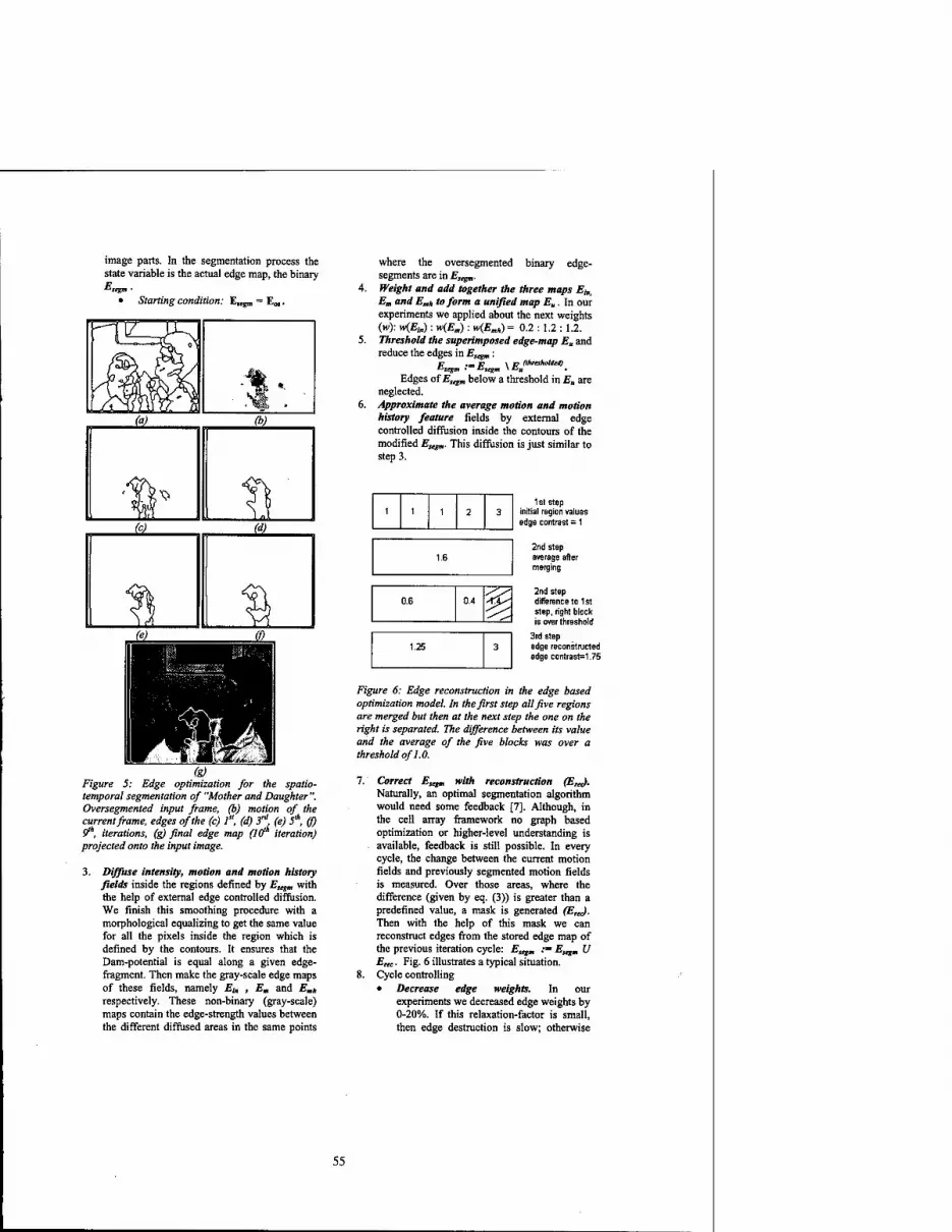
image parts. In the segmentation process the state variable is the actual edge map, the binary Escgm •

• Starting condition: t,ttfm = E„.

(a) (b)

Dt' (c) (d)

« t

Figure 5: Edge optimization for the spatio- temporal segmentation of "Mother and Daughter". Oversegmented input frame, (b) motion of the current frame, edges of the (c) ]", (d) 3rd, (e) 5", (f) 9*, iterations, (g) final edge map (W1 iteration) projected onto the input image.

3. Diffuse intensity, motion and motion history fields inside the regions defined by Eleg„ with the help of external edge controlled diffusion. We finish this smoothing procedure with a morphological equalizing to get the same value for all the pixels inside the region which is defined by the contours. It ensures that the Dam-potential is equal along a given edge- fragment. Then make the gray-scale edge maps of these fields, namely Ete , Em and Emh

respectively. These non-binary (gray-scale) maps contain the edge-strength values between the different diffused areas in the same points

where the oversegmented binary edge- segments are in Esegm. Weight and add together the three maps £/„, E„ and Emh to form a unified map Eu. In our experiments we applied about the next weights (w): H<E,„) : w(E„): w{EmH) = 0.2 :1.2 : 1.2. Threshold the superimposed edge-map E„ and reduce the edges in Estgm:

£.— IT \ 17 (threshotdal) segm --"stgrn 1*1

Edges ofEstgm below a threshold in E„ are neglected. Approximate the average motion and motion history feature fields by external edge controlled diffusion inside the contours of the modified E,egm. This diffusion is just similar to step 3.

1 1 1 2 3

1.6

0.6 0.4 -r^- -^V-

1.25 3

1st step initial region values edge contrast = 1

2nd step average alter merging

2nd step difference to 1 st step, right block is over threshold

3rd step edge reconstructed edge contrasts! .75

Figure 6: Edge reconstruction in the edge based optimization model. In the first step all five regions are merged but then at the next step the one on the right is separated. The difference between its value and the average of the five blocks was over a threshold of 1.0.

7. Correct Elegm with reconstruction (Era). Naturally, an optimal segmentation algorithm would need some feedback [7]. Although, in the cell array framework no graph based optimization or higher-level understanding is available, feedback is still possible. In every cycle, the change between the current motion fields and previously segmented motion fields is measured. Over those areas, where the difference (given by eq. (3)) is greater than a predefined value, a mask is generated (EreJ. Then with the help of this mask we can reconstruct edges from the stored edge map of the previous iteration cycle: E^m := Estgm U E„c. Fig. 6 illustrates a typical situation.

8. Cycle controlling • Decrease edge weights. In our

experiments we decreased edge weights by 0-20%. If this relaxation-factor is small, then edge destruction is slow; otherwise

55

the different regions merge into each other contours. Morphology operators may then be used faster. to get thin lines as a final result. Figs. 4 &5 show

• Go to step 3. some examples where the moving objects (and their According to our test results, approximately 10-15 shadow) are detected together. iterations were sufficient to get stable edge

An important issue is the execution-time of the above algorithm. Considering parameters of a VLSI 64x64 cell- array processor chip [6] (save/load of 64x64 image: 90nsec, arithmetic operation 0.5|xsec, logical operation: O.lilsec, convolution: 2\lsec) we can achieve 12msec total processing time, including several preprocessing steps of [10,11]. The cited experimental processor's technology (0.5|xm, 10MHz clock) is far from the available technological limits - but it still achieves high algorithmic speed at low power consumption of 1,2W.

4. Conclusion In our paper we outlined a fully-parallel spatio-temporal segmentation scheme based on small-neighborhood local computations and optimizations. The approach consists of two main modules: 1. Algorithms for motion estimation, segmentation and generating motion history map. 2. Contour-based split-and-merge spatio-temporal segmentation to utilize the information obtained in the first

module. Both parts can be realized with the same set of simple operations, the need for high-level control is minimized. Basic local instructions arc dynamic convolution operators, simple arithmetic steps, logical relations and the simplest nonlinear functions (sigmoid and gradient in a neighborhood). As we have found in the current and previous tests [12,13], these optimization algorithms are fast and give stable results in a reasonable number of steps. Our aims were to design optimal algorithms for fast implementation on parallel processor arrays. As time

complexity estimations show our approach can result in real-time operation, if implemented in VLSI. The parameters of the latest CNN chip have been applied to estimate the possible implementation of our complex system. This work proves that global (semi-global) optimization of very complex image analysis problems is possible through simple parallel functions interpreted in local neighborhood.

Acknowledgement: Special thanks are due to the Signal Processing Laboratory (LTS) of EPFL (in Lausanne). This work was supported by the Hungarian Research Fund (OTKA) and by the Swiss Research Fund.

References [I] T. Aach, A. Kaup, R. Mestcr: "Statistical model-based change detection in moving video", Signal Processing, Vol. 3i,

pp. 165-180, 1993. [2] P. Bouthemy and E. Francois: "Motion Segmentation and Qualitative Dynamic Scene Analysis from an Image Sequence",

Int. J. Comp. Vision, V. 10:2, pp. 157-182, 1993. [3] R. Dominguez-Castro et al.: "A 0.8um CMOS Two-Dimensional Programmable Mixed-Signal Focal-Plane Array

Processor with On-Chip Binary Imaging and Instructions Storage" IEEE Journal of Solid-State Circuits, Vol. 32, No. 7, pp. 1013-1026, 1997.

[4] M. Gelgon, P. Bouthemy: "A Region-Level Graph Labeling Approach to Motion-Based Segmentation", Technical Report, INRIA, 1996.

[5] K. Illgner and F. Müller: "Image segmentation using motion estimation", In V. Cappellini, editor, Time-Varying Image Processing and Moving Object Recognition, Vol. 4, pp. 238-243. Elsevier Science B.V., Amsterdam, 1997.

[6] G. Linan, S. Espejo, R. Dominguez-Castro, E. Roca: "A. Rodriguez-Vazquez: A Mixed Signal 64x64 CNN Universal Machine Chip", Proc. of MicroNeuro'99, IEEE, Granada, Spain, pp. 61-68, 1999.

[7] F. Moscheni, S. Bhattacharjcc, M. Kunt: "Spatiotcmporal Segmentation Based on Region Merging", IEEE Transactions on PAMI, Vol. 20, No. 9, pp. 897-915, 1998.

[8] P. Perona, T. Shiota, J. Malik: "Anisotropie Diffusion, Geometry Driven Diffusion In Computer Vision", Kluwer Academic Publishers, pp. 73-92, 1992.

[9] T. Sziränyi, M. Csapodi: "Texture Classification and Segmentation by Cellular Neural Network using Genetic Learning", Computer Vision and Image Understanding, Vol. 71, No. 3, pp. 255-270, September, 1998.

[10] T. Sziränyi, I. Kopilovic, B. P. Töth: "Anisotropie Diffusion as a Preprocessing Step for Efficient Image Compression", Proc. of the I4"1 ICPR, Brisbane, IAPROVEEE, Australia, pp. 1565-1567, August 16-20, 1998.

[II] T. Sziränyi, K. Läszlö, L. Czuni, F. Ziliani: "Object oriented motion-segmentation for video-compression in the CNN- UM", Journal of VLSI Signal Processing. V.23, No.2-3, pp.479-496, 1999.

[12] T. Sziränyi, J. Zerubia: "Markov Random Field Image Segmentation using Cellular Neural Network", IEEE CASI, Vol. 44, pp. 86-89, January, 1997.

[13] T. Sziränyi, J. Zerubia, L. Czuni, D. Geldreich, Z. Kato: "Image Segmentation Using Markov Random Field Model in Fully Parallel Cellular Network Architectures", Real-Time Imaging (Acad. Press), in press, 2000.

[14] Ä. Zarändy, et al.: "Implementation of Binary and Gray-Scale Mathematical Morphology", IEEE CAS I, Vol. 45. No.2. pp. 163-168, 1998.

56

2000 6™ IEEE International Workshop on Cellular Neural Networks and Their Applications Proceedings

Lossless Image Compression and Reconstruction by Cellular Neural Networks

Mamoru Tanaka, Yuichi Tanji,Miho Onishi and Toshiya Nakaguchi Dept. of Electrical and Electronics Eng.,, Sophia University,

7-1, Kioi-cho, Chiyoda-ku, Tokyo 102-8554 Japan Phone: +81-3-3238-3878, FAX: +81-3-3238-3321

email: tanaka@mamoru.ee.sophia.ac.jp

ABSTRACT: It is clear that the characteristic of cellular neural networks (CNNs) is the use of A-templates by which many kind of dynamical iterpolative nonlinear ef- fects can be generated without dependency of image scanning. This paper describes nonlinear quantization methods in a discrete-time cellular neural network(DT-CNN) . which generates a high quality lossy or lossless reconstructed image. It is very impor- tant that the DT-CNN state variable image which is determined dynamically based on the minimization of the DT-CNN Lyapunov energy function to generate an optimized interpolative predict function is a lossless interpolative DPCM image between the orig- inal input and the interpolation predict functions. The small compression ratio for the reconstructed lossless image can be changed by the multi-value quantization and the A-Template. By the DT-CNN non-dependency of image scanning, the lossless image points can be extracted even in an lossy image by checking the existence of local errors.

1. Introduction

Traditionally sequential explicit linear predictive coding has been used for lossless (reversible) compres- sion in such a standard JPEG DPCM method [1]. It is shown that in S(sequential Wavelet)+P(prediction)- transformation method [2] the S+P entropy (bits/pixel) whose mean is given by 4.65 is smaller than the JPEG entropy whose mean is given by 5.03 for many kinds of original images with 8 bits/pixels. The DPCM coding and decoding in the JPEG are done by using ordinary scanning. In the inverse 1-D wavelet transform of the S+P method, the lossless pixel value can be reconstructed by adding its prediction as a reverse scanning order for each of horizontal or vertical direction. These traditional methods for lossless image compression have advantage of reducing the number of scanning and computation time to solve the inverse orthogonal transformation in a sequential machine.

However, the explicit prediction methods have disadvantages that lossless pixels in low frequency local area can not be extracted for a lossy reconstructed image since the reconstruction depends on the scanning order. Also, since the prediction does not have optimal control to minimize the difference between original and prediction images in the coding system, there is possibility that the prediction is not efficient to reduce the lossless compression ratio.

The cellular neural networks(CNN's)[4] are used efficiently without the orthogonality to a lossy image compression and regeneration [3]. This paper describes nonlinear quantization methods in a discrete-time cellular neural network(DT-CNN) which generates a high quality lossy or lossless reconstructed image which has smaller compression ratio than the traditional methods.

The DT-CNN are described in matrix form as:

x(£ + 1) = Af (x(0) + Bu + T (1)

where x is a state variable vector, u is an input variable vector, f(x) is an output variable vector, A = [aij] and B = [bij] are feedback and feed-forward weight matrices which are able to represent by A- and B-templates respectively. The features of the DT-CNN are spatio-temporal dynamics by local connection, existence of high accuracy state variable and Lyapunov energy function, and use of programmable templates. Since linear and nonlinear filtering transformations by B-templates have been done traditionally by a conventional digital image processing, it is very important that the A-templates should be efficiently used by spatial combination of many cells to behave spatio-temporal halftoning. That is, the spatio-temporal dynamics by DT-CNN must generate nonlinear interpolative effects which have not been generated by a conventional image processing by a sequential machine.

The most important thing for DT-CNN image processing is in that the state variable x which is de- termined based on minimization of its Liapnov energy function to give an optimized interpolative predict function is a lossless interpolative DPCM image between the original input Bu and the interpolative predict value —Af(x). Therefore, the high quality lossy and lossless images can be reconstructed from simple decoding operation of B-1(—Af(x) + x). The compression ratio depends on the multi-value quan- tization and which region of the state variable x should be transmitted. The total lossless image can be obtained completely by the complete DPCM transmission for all regions of the state variable x which is quantized by using a quantizing function q(x) with same as slope as that of the input u.

0-7803-6344-2/00/$10.00 ©2000 IEEE 57

2. Hierarchical DT-CNN dynamics

The mapping from the state variable x to the multi-level quantizing function f(x) should not be done by conventional table memory because the accuracy of state valuable x is very high in CNN dynamical processing. The pixel quantization in a hierarchical DT-CNN can be constructed by a set of 1-bit cells(neurons), each of which has a nonlinear function of sign(x). That is, each pixel is constructed of sub-pixels according to an area intensity method. Each of sub-pixels is controlled by the corresponding 1-bit cell. The architecture by a set of 1-bit cells will be very efficient to make a base layer of chip and to change resolution and intensity of an image.

Let Cij be a local cell(LC) in a sub-pixel(t, j) with sub-area S(i,j), then a global cell(GC) C(I,J) in a pixel (/, J) with area S(I, J) is defined by

C(/,J) = {C0|i = l,2,.--,p;j = l,2,---,9} (2)

The global dynamics of each GC is described as follows:

xu(t+l) = J2 A{I,J;K,L)y±(K,L)(t)+ £ B(I,J;K,L)uKL + T C(K,t)ewr(;,j) c(K,L)eNr(i,J)

where the input UKL and the output y±(I,J)(t) are in the normalized interval [-1,1]. The output V±{I,J){t) is given by

where S±{I, J)(t) is a sighed pixel area which is defined as the area difference between the sum of ON sub-areas and the sum of OFF sub-areas in each pixel (/, J) by

S±(I,J) = Son(I,J)-S0„(I,J) (4)

J2 S{k,l)sign{xk,{t)) (5) ct,€C<;,j)

And the state valuable xu{t) is in the normalized interval [-xmax,xmaI] for T = 0 because

\xu\<xmax = J2 (\A(I,J;K,L)\ + \B{I,J;K,L)\ (6)

The local dynamics of each LC is described as follows:

Zy(t-t-l) = £ w(i,j;k,l)g(xki{i))+x,j(t+l) (7) Cj,;€P(/,J)

where the nonlinear function g{xki(£)) is given by

g(ikl(i)) = j^jrsign{xki{t)) (8)

for the weights

w(i,j,k,l)-y _s + s for{kl) = {iJ)

(9)

where the parameter 6 > 0 which defines the quantizing region of x is a parameter to be determined such that x = ±S for f(x) = ±1.

Though the local dynamics is not a Lyapunov stable, it converges almostly to a local equilibrium point by controlling the value of 6. Also, it is very important that the local dynamics converges absolutely to the optimal quantized value for 6 = 0 in the case that all weights w{i,j;k,l) are different, for example, •"('iJi^i') = 2',p = 0,1,2, • ■ • ,n- 1 like a sequential AD converter and that the number of iterations to converge can be reduced to at most n by adopting sequential order off-to-on transitions of the LC's. The convergent time of the local dynamics is sufficient enough to be done within each period of the global dynamics because they are performed in form of pipelining in the hierarchical DT-CNN.

58

fix) fix)

i

; -8 0

S X

Figure 1: Quantizing functions f(x)

The local dynamics for the weights w(i,j;k,l) = 2f,p = 0,1,2,• • • ,n- 1 and S = 0 generates a multi-level quantizing function defined by

f 1 (x>i

I -1 (z < -

(x>6)

■S)

(10)

flW f A([f + §]) (i is odd) I A([f]+' ] + |) (/is even)

A = 25

l-l

(11)

(12)

where A and ( are quantizing step and the number of quantized levels respectively and [ ] is a Gauss symbol. For example, the functions for / = 2, ( = 4 are shown in figures 1.

The Lyapunov energy function of the DT-CNN is defined by

Ei(t) = -^yT(A - D)y - yTBu - TTy.

where D = diag[(5]. Theorem 1 If A(J, J; K, L) = A(K, L; I, J) and

A{I, J; I,J)>0

(13)

(14)

then the energy function is a monotone decreasing function and the state variable x converges to a local stable equilibrium point.

Proof The energy function is written by

U,J) (*,|) (/,J)

Y, ]C B(I,J;K,L)y„(t)uKL - £ Ty,j(t) (15) (I,J) (K,L) (/.•>)

and is finite because of \yu{t)\ < 1 zju/jl < 1. In time t, Assume that the output of C(I, J) changes from yu{t - 1) to yu(t), Then the difference is given by Ay;j = y/j(t) - yu(t - 1). Let be

P = A[i Yl A(I,J;K,L)yij(t)yKL(t)+\ £ MK,L;I,J)yKL(t)yij(t)], (f,i) (K,L)

59

Ay <0

yii-i) yit-D

{yfi-D + j-Ay}

yti).

fix)

iy)

Figure 2: OUtput transition in the multi-quantizing function

then, since A(I, J; K, L) = A(K, L; I, J) for (K, L) ± (I, J), it is derived that

P = l-A(I, J; I, J)Ayu(t)2 + i Y, AV< J> K' L)&yu(t)yKL(t) iK.L)

+ \ £ MK,L;I,J)yKL(t)Ayu(t) (K,L)

= A(I, J; I, J){y,j(t - 1) + -Ayu + -Ayu - -Ayu}Ayu

+ Y,A(I,J\K,L)Ay,j{t)yKL(t) (K,L)

A(I, J; I, J){y,j(t) - -Ay,j}Ayu + £ A(I, J; K, L)Ayu(t)yKL(t) (K,L)

and

A^Syu(tf = 6{yu(t - 1) + -Ay,j}}Ayu. (16)

Including the case of (7, J; K, L) = (I, J; I, J) to the summation £, AE is given by

AE(t) = -[ J2 A{I,J;K,L)yKL+ . £ ... _B(7, J; K, L)uKL + T C(K,L)£Nr(I,J) C(K,L)eNr(r,J)

+->!(/, J; I, J)Ay,j - 6{y,j(t - 1) + ^Ayu}}Ayu

= -\xu - 6{yu{t - 1) + -Ayu} + 1.4(7, J; I, J)Ayij}Ay,j.

(17)

As shown in the figure 2, {yjj{t - 1) + \Ayu} in equation (17) is a center of the difference of the output y,j and its mapping to the x-axis is 8{yu(t - 1) + \Ayu}- By the definition of the function f{x), this mapped point is absolutely in the interval between xu(t - 1) and xu(t). When Ayu < 0, xu(t) is absolutely smaller than 6{yu(t - 1) + jAy/j}.

That is, since

xu < S{yu{t-1) + -Ayu} (18)

AE(t) < 0 is satisfied for A(I, J; 7, J) > 0. The case of Ayu > 0 is the same.

Proof End

3. Design for interporative DPCM by DT-CNN

Let G be a Gaussian filter, the high quality image can be reconstructed base on the distortion which i defined by

dist(y,u) = \\-yT{Gy-u)\\. (19)

60

x/

■U '1.0

"''/' /

vj IB 1.1

—V

Figure 3: slopes of quantizing functions

This distortion means that not only output value||y|| but also difference ||Gy — u)|| between the in- terpolative predict value and the reconstructed input image should be small. The interpolative predict Gy is corresponding to a lossy image. By the comparison between (13) and (19), the templates can be determined as

A = -G + diag{G}

T = 0

(20)

(21)

(22)

Next, we propose a new quantization method to transmit the state variable in form of lossy and lossless image compression based on an interpolative DPCM.

In the equilibrium point of the coding DT-CNN, the quantized state variable image is represented by

-Gf±\xt1Ji) + 6ff(xt™) + \ntl (23)

where the subscript and superscript in a variable v*b mean the slope and saturation value of the quan- tization function respectively. It is very important that the state variable x* ' (I, J) G xf1'5 which is determined based on minimization of DT-CNN Liapnov energy function to give an optimized interpolative predict functions is a lossless interpolative DPCM image between the original input ^uf1^, J) S ju*1

and the interpolation predict value of'(/, J) £ Gff a(x). As shown in the figure ??, the slope j of the

quantizing function fi{xf '5) is larger than that of the quantizing function of the input ufl and than

that of the transmitted state valuable xf1,s. The lossy image is generated by simple multiplication as

u* = Gff^xfx'5) (24)

through the transmission of the quantized state variable image x* for \\xjf || < 6 and x* = 1 for llxf 1-51I ^ $• The lossless image is generated by the operation

u'f1 = 2[Gf±I(x±1'5) +xf15 - ff^tx*1-5)] (25)

through the transmission of the complete quantized state variable image xf1'5. As a simulation, lossy and lossless images are obtained as shown in the figures 4(left) and 4(right)

respectively, in which a 5 x 5 Gaussian Template with 6 — 0.16 is used in the design. The mean of entropy (bits/pixel) in the lossless reconstruction is given by 4.61, though the optimized A-template is not designed yet statistically. It is very important here that almost state variables ^ are in the narrow region of [—6, S] as shown in the figure 3. and that the state value are divided to low frequency LL(-<5 < x{I, J) < 6), LH {5 < x{I, J) < l)and high frequency HH (1 < x{It J) < 1.5) images without dependency of sequential scanning. By its non-dependency of the scanning, the lossless image points can be extracted by checking the error 5ft 1(xf 15(K,L)) - x^15(K,L) = 0 in the neighborhood Nr(I,J)

even if we uses the lossy LL-image of Gf ikl(xf1,s) which has high quality except for shaping points like

character local images.

61

lossy image lossless image

Figure I,: Reconstructed images

0 20000 40000 60000 Phels

Figure 5: Size of State variables

4. Conclusions

It has been clear in this paper that, since the state variable is optimally determined based on the minimiza- tion of the distortion, the high quality lossy and lossless images can be reconstructed by simple operations in the proposed hierarchical DT-CNN. That is, what only CNN can do in the image processing is the nonlinear interpolative predictions by spatio-temporal dynamis without orthogonal transformations and without dependency of image scanning.

References

[1] M. Rabbani and P.W.Jones/'Digital Image Compression Techniques. Bellingham, WA:SPIE,1991.

[2] A.Said and W.A.Pearlman,"An Image Multiresolution Representation for Lossless and Lossy Com- pression", IEEE Tans, on Image Processing, Vol.5,No.9,Sep. 1996.

[3] M. Tanaka, K. R. Crounse and T. Roska, "Parallel Analog Image Coding and Decoding By Using Cellular Neural Networks", IEICE Trans. Fundamentals, VOL.E77-A, No.8 pp.!387-1395,August

[4] L. O. Chua and Lin Yang,"Cellular Neural Network:Theory" IEEE Transaction on Circuits and Systems, October 1988.

[5] M. Tanaka, K. Jin'no, J. Miyata, Masaaki Imaizumi, Toshiaki Shingu and Hiroshi Inoue, "Resolu- tionable Cellular Neural Networks", International Conference on Neural Networks(ICNN'97), Westin Galleria Hotel, Houston, Texas, USA, June 9-12, 1997.

62

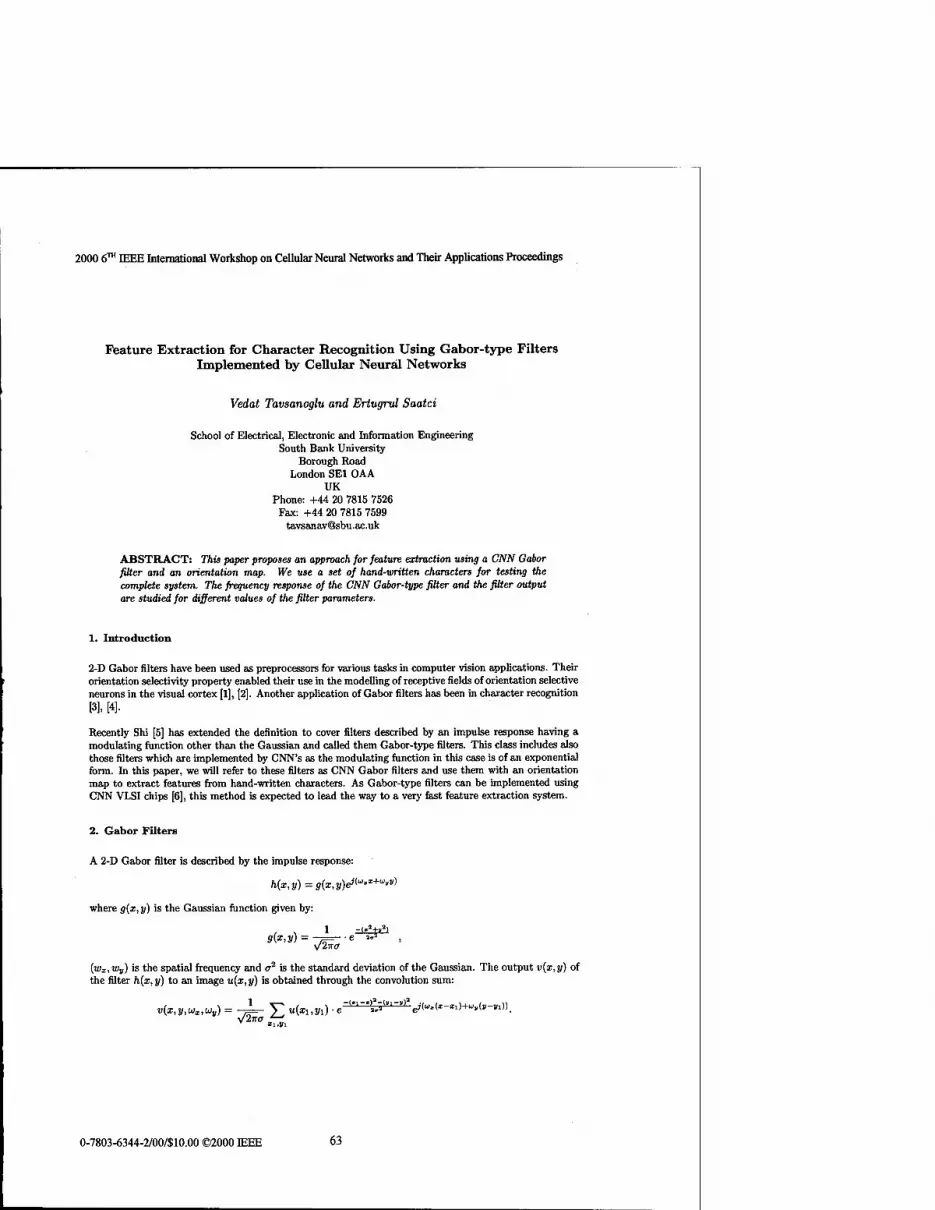
2000 6™ IEEE International Workshop on Cellular Neural Networks and Their Applications Proceedings

Feature Extraction for Character Recognition Using Gabor-type Filters Implemented by Cellular Neural Networks

Vedat Tavsanoglu and Ertugrul Saatci

School of Electrical, Electronic and Information Engineering South Bank University

Borough Road London SEI OAA

UK Phone: +44 20 7815 7526

Fax: +44 20 7815 7599 tavsanav@sbu.ac.uk

ABSTRACT: This paper proposes an approach for feature extraction using a CNN Gabor filter and an orientation map. We use a set of hand-written characters for testing the complete system. The frequency response of the CNN Gabor-type filter and the filter output are studied for different values of the filter parameters.

1. Introduction

2-D Gabor filters have been used as preprocessors for various tasks in computer vision applications. Their orientation selectivity property enabled their use in the modelling of receptive fields of orientation selective neurons in the visual cortex [1], [2]. Another application of Gabor filters has been in character recognition [3], [4].

Recently Shi [5] has extended the definition to cover filters described by an impulse response having a modulating function other than the Gaussian and called them Gabor-type filters. This class includes also those filters which are implemented by CNN's as the modulating function in this case is of an exponential form. In this paper, we will refer to these filters as CNN Gabor filters and use them with an orientation map to extract features from hand-written characters. As Gabor-type filters can be implemented using CNN VLSI chips [6], this method is expected to lead the way to a very fast feature extraction system.

2. Gabor Filters

A 2-D Gabor filter is described by the impulse response:

h(x,y) = g{x,y)e*»**+»*rt

where g(x,y) is the Gaussian function given by:

V27TCT

(u)x,wv) is the spatial frequency and <r2 is the standard deviation of the Gaussian. The output v(x,y) of the filter h(x,y) to an image u(x,y) is obtained through the convolution sum:

.(*,»,«.,«,) = -J=- £ u(x1,yi)-e-^-'&">-"feJ^*-*^y->^.

0-7803-6344-2/00/S10.00 ©2000 IEEE 63

3. CNN Gabor Alters

For the filtering of an M x A' pixel 2-D image. u(m,n) € R where m 6 {0,1,.... M — 1} and n € {0,1,..., A' - 1}, we use a 2-D CNN array of M x N cells where the state at the (m,n)th cell v(m,n) € C satisfies [5]:

p

v(m,n) = 2_. Ok,iv(m +k,n + l) + bu(m,n) (1)

where dot denotes differentiation with respect to time. The A = [ak,i\pk (__„ and b are complex coefficients called the feedback and feedforward cloning templates and p is defined to be the connection radius.The feedback cloning template is represented by a (2p + 1) x (2p + 1) matrix where the center element equals a0,0. For p = l, the cloning template matrix is:

A = 0-1,1 «0,1 Ol,l

0-1,0 OO.O Ol,0

0-1,-1 Oo,-1 Ol,_l

In the case of 2-D low-pass CNN Gabor filter, feedback cloning template A is given by Shi as:

A-- 0 1 0 1 -(4 +A2) 1 0 1 0

For any 2-D low-pass CNN Gabor filter there corresponds a 2-D band-pass CNN Gabor filter tuned to the centre frequency {wxo, wv0) obtained by replacing the feedback cloning template with

A = [at,,e" J(te,„+lu-,«)

A = 0 e~lu''0 0

e>«.-.o _(4 + A2) e-'

u" 0 e'u'"° 0

(2)

Its frequency response is obtained by shifting that of the low-pass filter to the spatial frequency (to,,, wyo).

In order to obtain the frequency response of the cells we use eqn.l. If the filter is stable, it does not oscillate and eventually settles to a stable equilibrium point for which eqn.l takes the form [7]:

7] ai,,iv(m + k,n + l) + bu(m,n) = 0 *,(=-i

Under this condition we write v(m,n) as

-1 , v{m,n) = [o_i ov(m — l,n) + ao ii)(m,n + 1) + Oi o"("i + l,n) + oo -\v(m,n — 1) + bu(m,n)]

Go,o

Using the feedback template in (2) and choosing the feedforward cloning template as b = A2, we obtain

v(m,n) — 1

4 +A2 [e'WMv(m-\,n)+e~>w'°v(m,n+\)+e~'w-Him+\,n)+e'w'°v(m,n-\)+bu{m,n)} (3)

The two-sided 2-D Z transform of both sides of (3) yields

V(zm,zn)[(A + A2) - e>*'°z-1 - e-'w"zn - e->'"-°zm - e^z"1] = A2C/(zm, z„) (4)

Evaluating (4) at zm = e'w' and zn = e'u", we obtain the frequency response of the CNN filter:

„ . _ V(ei"',e'm') A2

H(c's

U(e'Wi,e>w>) 4 + A2 — 2cos(wx — wxo) — 2cos(wy — Wyo) (5)

64

For a circuit implementation of this network, the complex-valued state v(m,n) is represented by the voltage across two capacitors representing its real and imaginary parts vr(m,n) and Vi(m,n). Substituting (2) into (1) and separating real and imaginary parts, we can express the time evolution of the complex-valued state in (1) as an equivalent system where the complex state variable has been replaced by two real-valued state variables:

l>r | _ | COSWzO

Vi

„„ -sinu/so 1 f vr(ro-l,n) 1 [ cosio„o sintu„o 1 [ vr(m,n + l) sinwx0 COSTOI0 J [ v4(m-l,n) j [ -sinu>„0 costu„o j [ Vi(m,n + 1)

coswx0 sintol0 1 [ vr(m + l,n) 1 [ cosw„o -sintu^o 1 [ vr(m,n-\) -sinwzo cosw„o J L Vi(m + l,n) J [ sint«„o cosw„o J L Vi(m,n-l)

(4 +A2) 0 1 [ vr(m,n) } \ A2u(ra,n) 0 (4 + A2) J [ Vi(m,n) j + [ 0

4. Orientation Map

Gabor niters are orientation selective and respond maximally to edges which are oriented at an angle 9 = atan(wvo/wxt)) where 6 is defined to be the angle between the horizontal axis and the line perpendicular to the edge. In order to detect the angle 9 of a particular orientation in an image, we use a filter bank of np Gabor filters whose spatial frequencies are:

{(wkx0 = TCOs9k,w

kv0 = Tsin9k) | 9* = — ,fc = 0,---,(np - 1)} (6)

where r is the radius of spatial frequency. The angle 9k associated with the filter of the maximum output is taken as the orientation of the particular edge in the image.

In order to make use of the Gabor filter output we convert it to an orientation map [8] where the vertical and horizontal axes represent the total orientation and the angle of orientation, respectively. Here the total orientation at an angle of orientation is obtained as the sum of pixel orientations taken over all the pixels in the image with the same angle of orientation.

The Dominant Orientation Matrix for each pixel is found by comparing the orientations of the same pixels of the filter outputs. The comparator finds for each pixel the maximum orientation, i.e.

max{vk(m,n,9k)} over all k

A pixel at the output of the comparator is then assigned the value of k for which it received the greatest value. The matrix associated with the m x n output of the comparator is called the dominant orientation matrix. The total orientation is calculated to be the number of pixels in the image with the same angle of orientation. The number of pixels with same dominant orientation in the dominant orientation matrix is counted and assigned as orientation value for that particular orientation angle. The orientation map is defined as the graph of sum of dominant orientations versus orientation angles.

5. Selection of r and A

Considering (5) and (6) reveals that r is the radius of spatial frequency controls the location of Gabor filter centre frequency (wxo,Wyo)- On the other hand, the parameter A determines the spread of the CNN Gabor filter frequency response along both 9 and 9 + 90 directions, which are the same due to the circular symmetry of the filter. Small selection of A makes the filter narrow and selective which yields better results. Hence the appropriate choice for the parameters r and A is crucial in CNN Gabor filtering. The values for these parameters should be chosen such that most of the energy is captured by the filter. Only in this case steering the filter by changing 9 results in significant variations of the filter output. The FFT's of selected four handwritten characters are shown in Fig.5. It is easily seen that most of the energy is

65

localised at lower frequencies. Therefore values of r should be chosen small enough to capture most of the energy on the frequency plane. When the spectrum of the Gabor filter matches mast of the frequency spectrum of the character maximum response from the filter will occur.

6. Example

In this paper we use a filter bank of np = 18 filters to detect the dominant orientation. The first task is to assign values to the parameters A and r of this system. To this end, we prepare the circle pattern shown in Fig.4. As the circle consists of edges with all orientations distributed equally, we should expect to obtain an almost flat orientation map when input pattern is a circle. Therefore such an input sets a good example of a test pattern for finding appropriate values for r and A. The orientation map for the circle (or letter "0") in Fig. 4a is shown in Fig.4b-4c. In this case after a few trials, we have reached the values r = 1.1 and A = 0.1. The letters "A","L","I","0" and their orientation maps are depicted in Fig.l - 4, where A = 0.1, for r = 0.1 and r = 1.1 respectively. Also Fig. 6 shows the frequency response of these filters for 6 = 2TT/9. Fig. 7 (a) and (b) show the orientation map of letter "A" for A = 0.1, r - 2.5 and the frequency response of CNN Gabor filter for A = 0.1, r = 2.5 and 0 = 2^/9. In this case as one of the filter parameters has not been given a suitable value, namely r, the orientation map obtained as a result of the filtering does not represent the actual character.

7. Conclusion

In this study feature extraction from handwritten characters has been carried out using Gabor-type filters implemented by CNN's. An orientation map is used which converts the filter output to a suitable form of extracted features. Filtering is investigated using different parameter values and optimum parameter values have been discussed. The result of this study is will be used in handwritten character recognition using CNN Gabor filters.

8. References

[1] Marcelja S. "Mathematical Description of the Responses of Simple Cortical Cells", Journal of the Optical Society of America, vol.AO, no.ll, pp.1297-1300, 1980.

[2] Daughman J.G. "Two-dimensional spectral analysis of cortical receptive field profiles", Vis. Res.. vol.20, pp.847-856, 1980.

[3] Hamamoto Y., Uchimura S., Watanabe M., Yasuda T. and Tomita S. "Recognition of Handwritten Numerals Using Gabor Features", IEEE Proceedings of ICPR'96, pp.250-253, 1996.

[4] Deng D., Chan K.P., Yu Y. "Handwritten Chinese character recognition using spatial Gabor filters and self-organizing feature maps", IEEE Interrnational Conference, Proceedings ICIP-94. vol.3, pp.940-944 1994.

[5] Shi B.E. "Gabor-Type Filtering in Space and Time with Cellular Neural Networs", IEEE Trans, on CAS-I,vol45, 2, pp.121-132, February 1998.

[6] Shi B.E., "2D Focal Plane Steerable and Scalable Cotical Filters", Proceedings of the Seventh International Conference on Microelectronics for Neural Fuzzy and Bio-Inspired Systems. MicroNeuro'99, pp.232-239, 1999.

[7] Shi B.E. and Chua L.O., "Resistive grid image filtering: input/output analysis via the CNN framework", IEEE Trans. Circuits Syst. I, Vol.39, pp.531-548, July 1992.

[8] Tufan E., Tavsanoglu V., Cekli E. and Ozmen A., "Characterisation of Handwritten Characters using Streeble Filters" (in Turkish), Turkish National Symposium on Signal Processing and Application SIU'98, Ankara, Turkey, 1998.

66

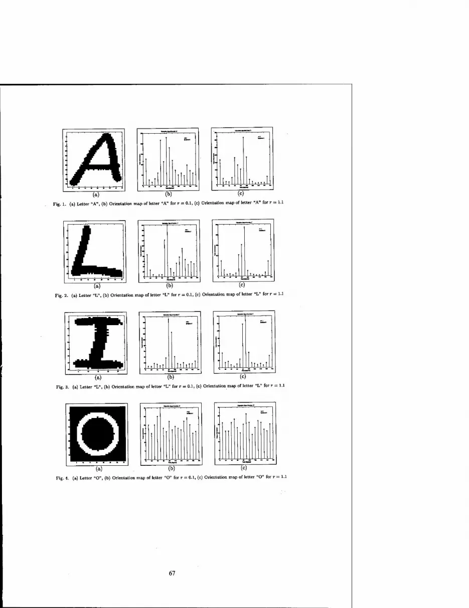
(a) "(b) (c)

Fig. 1. (a) Letter "A", (b) Orientation map of letter "A" for r = 0.1, (c) Orientation map of letter "A" for r = 1.1

(a) (b) (c)

Fig. 2. (a) Letter "L", (b) Orientation map of letter "L" for r = 0.1, (c) Orientation map of letter "L" for r = 1.1

ttltll LLLLU

»—

1" !■

lll.tl llhllll ■ " " " -—

(a) (b) (c)

Fig. 3. (a) Letter "L", (b) Orientation map of letter "L" for r = 0.1, (c) Orientation map of letter "L" for r = 1.1

(a) (b) (c)

Fig. 1. (a) Letter "O", (b) Orientation map of letter "O" for r = 0.1, (c) Orientation map of letter "O" for r = 1.1

67

(a)

(c) (d)

Fig. 5. (a) FFT of letter "A", (b) FFT of letter "L", (c) FFT of letter "O", (d)FFT of letter "I"

Fig. 6. (a) Frequency Response of the CNN Gabor Filter for r = 0.1, A = 0.1 and $ = 2u/9, (b) Frequency Response of the CNN Gabor Filter for r = 1.1, A = 0.1 and $ = 2n/9.

Fig. 7. (a) Orientation map of letter "A" for r = 2.5, (b) Frequency Response of the CNN Gabor Filter for r = 2.5, A = 0.1 and 6 = 2JI/9.

68

2000 6™ IEEE International Workshop on Cellular Neural Networks and Their Applications Proceedings

Subthreshold Implementation of a 2D CNN Gabor-type Focal Plane Filter

Bertram E. SHI

Department of Electrical and Electronic Engineering, Hong Kong University of Science and Technology, Clear Water Bay, Kowloon, Hong Kong, tel: +852 2358 7079, fax: +852 2358 1475,

email: eebert@ee.usthk

ABSTRACTS We describe the implementation of a focal plane CNN array for computing the outputs of orientation selective filters similar to Gabor filters using weak inversion tran- sistor circuits. Both the scale and the orientation selectivity of the filter can be tuned elec- tronically. We exploit the concept of the transistor as a pseudo-conductance or diffuser and use current, rather than voltage to represent signals of interest. This design enables energy efficient computation of the filter responses. Test results from a 12 x 14 pixel array fabri- cated in 1.2\lm technology are presented.

1. Introduction

We have reported implementations of ID and 2D focal plane implementations of cellular neural network (CNN) Gabor-type filters based on strong inversion transistor circuits[l][2]. The filters have complex valued impulse responses which are complex exponentials modulated by a low pass function. In the 2D case, these filters are ori- entation selective, where the tuned orientation is determined by the direction in which the complex exponential is oscillating. The scale or width of the filter is determined by the magnitude of the spatial frequency and the band- width of the filter. Both the orientation and scale can be tuned electronically by adjusting external bias voltages. Processing circuits are analog, operate in continuous time and pixel parallel.

Here we describe the implementation of these filters using weak inversion transistor circuits. Andreou et. al. note that the energy efficiency is maximized when transistor operate in weak inversion. We exploit the concept of the transistor as a pseudo-conductance or diffuser and use current, rather than voltage to represent signals of inter- est

2. Pixel Architecture

For clarity, we assume ID images at first The extension to 2D is given at the end of this section. Given a real valued input image w(n), the complex valued filter output i(n) minimizes the cost function

E(i) = IZl'M-^uM^+^^ZliM-e'^iim+nl2

m m

where Ha, Si and Afl are constants. This cost function is the sum of two terms: a data fidelity term which penal- izes the difference between the filter output and the input scaled by Ha and a regularization term which is mini- mized if the output is a complex exponential waveform with spatial frequency Si. The amount each term contributes to the cost function is controlled by Ali.

By differentiating the cost function above with respect to the real and imaginary parts of i(n) (ir(n) and i,<n)) and setting the results equal to zero, we find at each pixel,

0 = ajjfa -1) - (Ho1 + 2o.{)ir(n) + a^'/n + 1) - a2i,<n -1) + a2i,(n + 1) + u(n)

0 = ajf/i - 1) - (Hsl + 2al)iI{n) + ajfa + 1) + a2ir(n - 1) - a2ir(n + 1)

where

_ cosn _ sinfl _ Hq "' " (&.SiYHa

Ul ~ (Aß)2fffl H° ~ 2-2cosa (l)

+ (AQ)2

Assuming an infinite array and applying the discrete Fourier transform, we can show that i(n) is the result of applying a filter with transfer function

Ho H(0)) =

. 2-2cos(w-ft) 1 + -

(Afi)2

0-7803-6344-2/00/$ 10.00 ©2000 IEEE 69

This filter is bandpass with center frequency A and 6dB half bandwidth approximately equal to Afl. The gain at the center frequency is Ha, The gain at DC is H0. The impulse response of this filter is approximately

h(n) = Hn^e-AimMe;a-

A circuit implementation of the filter can be obtained by using KCL to implement the summations in (1). Each pixel has two nodes corresponding to the two summations. Previous voltage mode designs represented w(n) as current, i£ri) and i,{ri) as voltages and used linear transconductance amplifiers and resistors to implement the coefficients. This design represents both u(n) and i(n) as currents and uses current amplifiers and MOS transis- tors operating as "pseudo-conductances" or "diffusers"[3][4].

If HB = 1, then the first line of each summation can be implemented by the circuit shown in Fig. 1(a) where we assume that the transistors operate in weak inversion. The difference between Vh and Vv controls the value of «i =

VT denotes the thermal voltage, K denotes a constant less than 1. The second line of the sums are implemented using current amplifiers which sense the currents leaving the

drains of the transistors M„. Fig. 1(b) shows the circuits associated with two interior pixels in the array and a pixel at the left edge. The bias currents /bi„ enable the response to u(n), which is actually the difference between the drain currents of Mv and /bi„, to assume both positive and negative values. Fig. 1(c) shows the transistor level schematic of the current amplifier. The diode connected transistors are also mirrored to enable read-out of the currents ir(n) and i,(n). The gain Oj depends exponentially on the difference between source voltages Vsl

andVs2. The currents u(n) are supplied by a photodetector stage consisting of a vertical PNP phototransistor formed by

the diffusion/well/substrate junctions and a PMOS mirror.

■t !>-!)■

I?

© © ©

I»'

if v'-H[S XriL"' TrC i>+D

plC* vT pl[V VT pj[V VT

<•,<<>) i,(D i,<2)

(a)

[%"• vT f»^ vT rt*- vT ir(0) <V(D i/2)

(c) (b)

Fig. 1: (a) A weak inversion transistor network where the relationship between the currents is linear, (b) The circuits associated with two pixels of the array in the interior (pixels 1 and 2) and one pixel at the left edge of the array (pixel 0). (c) The transistor implementation of the current amplifiers.

70

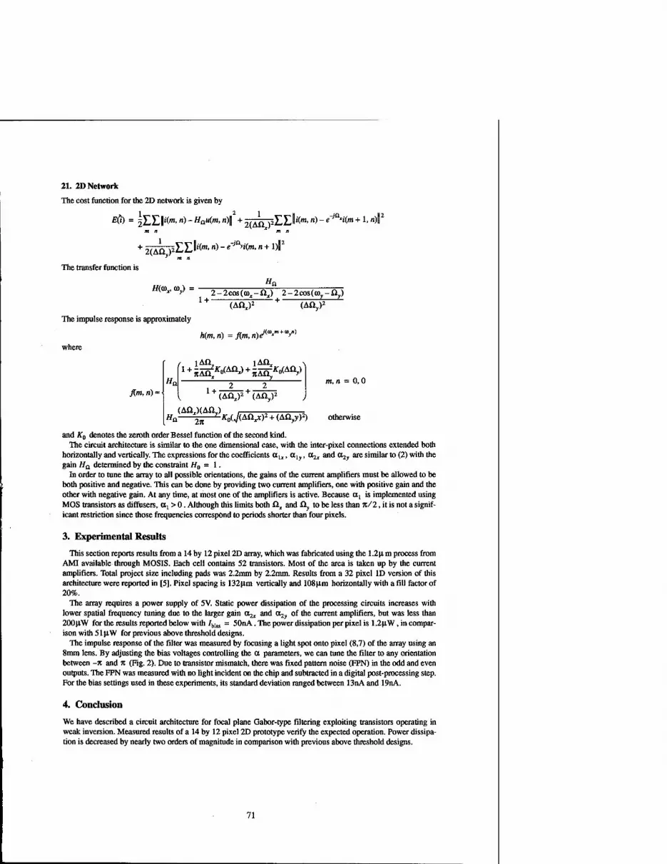
21. 2D Network

The cost function for the 2D network is given by

£<>) = jEEi*». n> - H^m- ">12+scA^pEE'*"'n) ~ *J^°"+L n)'2 m n x m n

;£ll'("«>n)-e-^.(m,n+l)l2

2(Aiy

The transfer function is

//(CD,, CO,) =

The impulse response is approximately

Ha

2~2cas(<ax-£lx) 2-2cos(co),-fl),) 1+ (Ä7£j* + (Afly)2

A(m,«)=/tm>n)e''(0,'m + 'V0

where

fl.m,n)-- Hc

f lAft lAß

1 + :

(AflJ(Anv) , Ha ^-^/foC^Aß^)2 + (Afl,y)2)

0,0

otherwise

and Af0 denotes the zerofh order Bessel function of the second kind. The circuit architecture is similar to the one dimensional case, with the inter-pixel connections extended both

horizontally and vertically. The expressions for the coefficients ou, aly, a^, and a.2y are similar to (2) with the gain Ha determined by the constraint H0 = 1.

In order to tune the array to all possible orientations, the gains of the current amplifiers must be allowed to be both positive and negative. This can be done by providing two current amplifiers, one with positive gain and the other with negative gain. At any time, at most one of the amplifiers is active. Because aL is implemented using MOS transistors as diffusere, aL > 0. Although this limits both ilx and Ciy to be less than Jt/2, it is not a signif- icant restriction since those frequencies correspond to periods shorter than four pixels.

3. Experimental Results

This section reports results from a 14 by 12 pixel 2D array, which was fabricated using the 1.2u. m process from AMI available through MOSIS. Each cell contains 52 transistors. Most of the area is taken up by the current amplifiers. Total project size including pads was 2.2mm by 2.2mm. Results from a 32 pixel ID version of this architecture were reported in [5]. Pixel spacing is 132u,m vertically and 108um horizontally with a fill factor of 20%.

The array requires a power supply of 5V. Static power dissipation of the processing circuits increases with lower spatial frequency tuning due to the larger gain a^ and a2y of the current amplifiers, but was less than 200jiW for the results reported below with IVm = SOnA. The power dissipation per pixel is 1.2 u,W, in compar- ison with 51 p-W for previous above threshold designs.

The impulse response of the filter was measured by focusing a light spot onto pixel (8,7) of the array using an 8mm lens. By adjusting the bias voltages controlling the a parameters, we can tune the filter to any orientation between -7C and TC (Fig. 2). Due to transistor mismatch, there was fixed pattern noise (FPN) in the odd and even outputs. The FPN was measured with no light incident on the chip and subtracted in a digital post-processing step. For the bias settings used in these experiments, its standard deviation ranged between 13nA and 19nA.

4. Conclusion

We have described a circuit architecture for focal plane Gabor-type filtering exploiting transistors operating in weak inversion. Measured results of a 14 by 12 pixel 2D prototype verify the expected operation. Power dissipa- tion is decreased by nearly two orders of magnitude in comparison with previous above threshold designs.

71

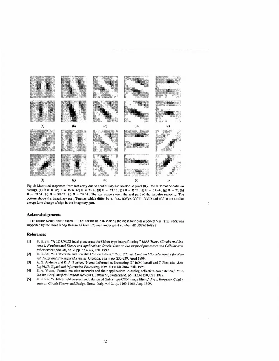
Ufa ÜKB

(a) (c) (d) (c)

■

(0 (g) (h) (>) (j)

Fig. 2: Measured responses from test array due to spatial impulse located at pixel (8,7) for different orientation tunings, (a) 8 = 0. (b) 8 = it/8 . (c) 8 = tt/4. (d) 8 = 3TC/8 . (e) 8 = 7C/2. (f) 8 = 37C/4. (g) 8 = Jt. (h) 8 = 57t/4. (i) 8 = 371/2. (j) 8 = 77T./4. The top image shows the real part of the impulse response. The bottom shows the imaginary part. Tunings which differ by 7C (i.e., (a)/(g), (c)/(h), (e)/(i) and (f)/(j)) are similar except for a change of sign in the imaginary part.

Acknowledgements The author would like to thank T. Choi for his help in making the measurements reported here. This work was

supported by the Hong Kong Research Grants Council under grant number HKUST6216/98E.

References

[1] B. E. Shi, "A ID CMOS focal plane array for Gabor-type image filtering," IEEE Trans. Circuits and Sys- tems-I: Fundamental Theory and Applications, Special Issue on Bio-inspired processors and Cellular Neu- ral Networks, vol. 46, no. 2, pp. 323-327, Feb. 1999.

[2] B. E. Shi, "2D Steerable and Scalable Cortical Filters," Proc. 7th. Int. Conf. on Microelectronics for Neu- ral, Fuzzy and Bio-inspired Systems, Granada, Spain, pp. 232-239, April 1999.

[3] A. G. Andreou and K. A. Boahen, "Neural Information Processing II," in M. Ismail and T. Fiez, eds., Ana- log VLSI: Signal and Information Processing, New York: McGraw-Hill, 1994.

[4] E. A. Vittoz, "Pseudo-resistive networks and their applications to analog collective computation," Proc. 7th Int. Conf. Artificial Neural Networks, Lausanne, Switzerland, pp. 1133-1150, Oct. 1997.

[5] B. E. Shi, "Subthreshold current mode design of Gabor-type CNN image filters," Proc. European Confer- ence on Circuit Theory and Design, Stresa, Italy, vol. 2, pp. 1163-1166, Aug. 1999.

72

2000 6™ IEEE International Workshop on Cellular Neural Networks and Their Applications Proceedings

Analogic Computing: System aspects of Analogic CNN Sensor Computers

Tamäs Roska

Analogical and Neural Computing Laboratory of the Computer and Automation Research Institute of the Hungarian Academy of Science, Budapest and the

Department of Information Technology, Pazmäny P. Catholic University, Budapest address: Kende u. 13, Budapest, Hungary H-l 111

phone: (+361) 2095263, fax: (+361) 2095264, email: roska@sztaki.hu

ABSTRACT: A new principle of computing and computers is emerging: the analogic cellular computer. Its architecture, the CNN Universal Machine, is now implemented in several different physical forms and the first practical experiments exhibit breathtaking frame rate and computing power. Several "Kilo real-time video" frame rate (more than 10,000 frames per second) and TeraOPS computing power on a 1 cm CMOS (0.5 micron) chip were measured. In this review article, the systems aspects and the new directions in this field are considered. A new world of software and a new notion of computing are taking ground. The possibility of software in optical computing becomes feasible. Likewise, programming on atomic and molecular scale implementations may be possible. Hence, photons and molecules may be used for signal representation in these analogic computers.

1. Scenario

Recent history of the electronic and computer industry can be viewed as three waves of revolutionary processes [1]. The first revolution, making cheap computing power available via microprocessors in the 70s, led to the PC industry of the 80s. The cheap laser and fiber optics which resulted in cheap bandwidth at the end of the 80s led to the Internet industry of the 90s. The third wave, the sensor revolution at the end of the 90s, will also provide for a new industry. Sensor revolution means that cheap sensor and MEMS (micro electro mechanical system) arrays are proliferating in almost all conceivable forms. Artificial eye, nose, ears, taste, and somatosensory devices as well as sensing all physical, chemical and biological parameters, together with microactuators, etc. are becoming commodities. Thousands and millions of generically analog signals are produced waiting for processing. A new computing paradigm is needed. The cited technology assessment [1] reads: "The long-term consequence of the coming sensor revolution may be the emergence of a newer analog computing industry in which digital technology plays a mere supporting role, or in some instances plays no role at all". I do think that for processing analog array signals, the Analogic Cellular (CNN) Computer paradigm, based on the CNN Universal Machine architecture and its various physical implementations, is a major candidate to play this role. At the same time, Analogic Cellular Computers mimic the anatomy and physiology of many sensory and processing organs, even with stored programmability. Recent studies on optical and nano scale implementations open up new horizons on the atomic and molecular levels. Stored programmability, invented by John von Neumann, was the key for endowing digital computers with an almost limitless capability within the digital universe of signals, opening the door to human invention via digital algorithms and software. Indeed, according to the Turing-Church Thesis, any algorithms on integers conceived by humans can be represented by Recursive functions/Turing Machines/Grammars. The CNN Universal Machine is universal not only in a Turing sense but also on analog array signals. Due to stored programmability, it is also open to human intelligence with a practically limitless capability within the universe of analog array signals, via analogic spatiotemporal algorithms and software.

Optical implementation is already emerging using molecular level analog optical memory (Bacteriorhodopsine or polimer materials) [8,9]. Atomic and molecular level implementation of the CNN array as well as the CNN-Universal Machine may become feasible. The Analogic Cellular Computer represents a new platform for computing, however, this notion of computing contains brand new elements and techniques as well, partially reflecting some forms of nature-made information processing.

Nature-made information processing has several different manifestations. On the Molecular level this means the protein structures or interacting molecules on a two or three dimensional grid; on the Neuronal level it may mean the many sensory organs and subsequent neural processing. On the Functional neuronal level it may mean the information representation in spatiotemporal memory, the functional laterality of the brain, as well as the parallel processing places and functional units

0-7803-6344-2/00/S10.00 ©2000 IEEE 73

learned via PET, NMR, fNMR, etc. On the Mathematical-Physical level, it may mean several dynamic spatio-temporal processes and phenomena represented by different nonlinear Partial Differential Equations (PDEs). The striking intellectual and scientific challenge is: how to combine these diverse phenomena in useful algorithms running on a standard spatio-temporal computer, based on the CNN Universal Machine. The surprising fact is that it can be done, based at least on some examples and experiments.

1 stored program on integers (e.g. digital numbers and symbols)

stored program on fbws (e.g. image sequences and symbols)

Figure 1. The Digital and the Analogic Universe in Stored Programmable Computing.

2. Kilo real-time and Tera OPS on an Analogic Visual Microprocessor

The computational power of this new technology is breathtaking. There are two classes of problems where no other technology can compete.

74

Class K: Kilo real-time [K r/t] Same rate class. The frame rate of the process in this class is in the order of about thousand times faster than the real-time video frame rate (30 frame per second). A typical experiment is reported in [14] where a pattern classification with more than 10,000 frames per second was tested (more than 0.33 K r/t). Using current CMOS Technology, 1.5 K r/t, that is about 50,000 frame per second is feasible. In this Class K, the high frame rate is the key in the computation. Clearly, the sensing and computing tasks are to be physically integrated. In standard digital technology, there is no time for A to D conversion and to complete the calculation, all within the few microsecs.

Class T: TeraOPS equivalent computing power class. Even if the frame rate is small, like real/time video (30 frame per second), the required computing power (per chip) is enormous. Indeed, Trillion operations per second is to be, and can be, achieved [6, 12]. These TeraOPS chips are capable to solve a nonlinear PDE on a grid in a few microsec. The detection of a moving inner boundary of the left ventricle in an echocardiogram, via an analogic CNN algorithm [13] combining several waves, local logic, and morphology operators, took only 250 microsec on the ACE4K analogic Visual Microprocessor Chip made in Seville, These chips hosted 4096 cell processors on a chip. This means about 3 TeraOPS equivalent computing power which is about thousand times faster than the computing power of an advanced Pentium processor.

3. The world of analogic algorithms using Spatial-temporal Instruction Set Computers (StISC)

The signals to be processed are two-dimensional (2D) signal arrays or image flows. The 2D array may represent pictures or any other 2D sensory output signals of continuous value in continuous time. 3D arrays of signals can be defined similarly. Without loss of generality we will discuss 2D image flows, or video flows, the only discretization is in space. The formal framework of analogic computing is as follows [26]. A finite time image flow <S> (t) is defined as:

*(t):{<fcj(t). t€T=[0,td]}

lSi<m l<j <n

where m and n are positive integers, td > 0 (time duration), <j% (t) e C' (continuously differentiable). For example, <p,j may represent an input, state, or output of a cell (representing a pixel) in an m x n cell array, and % (t) is bounded.

At t = t*, * (t*) is an m x n Picture (a snapshot),

P: {pij e R1} , I Pij I < pm„ e R' < ~, where pi; is the pixel intensity .

Without loss of generality we may assume that in a gray scale image black and white are represented by +1 and -1 (or +1 and 0). In this paper we will use the +1 and -1 convention. A color picture is represented by a combination of several color layers of mxn cell arrays, each layer is representing the intensity of the appropriate color component (e.g. R,G,B).

A binary picture can be called a mask M,

{1,-1} M: niij e or

{1. 0}

A sequence of snapshots at t=to, to + At, to + 2At to + kAt is called image sequence or video stream, denoted by <D (k). A spatial-temporal instruction set computer (StISC computer) operates on image flows, or image sequences, the elementary instruction is defined as

*.u«pu. (t):= * (*i„pu.(t), t € T = [0, td] (1) or Oou,pu,(k):= ¥(*lnpu,(k), t=l,2,... 4* being a function on image flows or image sequences. As an example, a video clip is transformed into another video clip.

75

A functional F on an image flow is defined as

P: = F(<J>,„p,„(t)) (2)

As an example, an image flow or a video clip is transformed into a picture showing the maximum intensity values in each pixel.

The output image could be a mask, M, as well. For example, the mask pixel would be black if a change occurred in O (t).

If after t = td the output is not settled, i.e. there exists at least one ij -> <p,j (t) * 0

then the spatial-temporal dynamics or the equivalent spatial-temporal instruction is of non-equilibrium type.

The next question is how to build a computer with non-equilibrium type elementary instructions, i.e. the StISC computer (also called analogic cellular computer).

The StISC Computer should perform • non-equilibrium type spatial-temporal elementary instructions, • spatial logic instructions on spatial masks, acting pixel-wise (e.g. a cellular automaton), • spatial-temporal combination of image flows and/or pictures pixel-wise, and • algorithms (recursive functions) using the above three types of instructions. The algorithms defined in this way are called

non-equilibrium spatial-temporal (NEST) algorithms.

Remark 1: Spatial-temporal instructions with settled output are special cases. Remark 2: Loosely speaking, the usual analogic CNN algorithms belong to this class. Remark 3: The Cellular Neural/nonlinear Network (CNN) is a minimal and powerful representation of a non-equilibrium type spatial-temporal (NEST) elementary instruction. Once the cell is selected the parameters are: • the cloning template • input, initial state, output (bias map, fixed state) • time duration (td) • boundary condition Remark 4: The CNN Universal Machine (CNN-UM) architecture is a minimal and in a sense universal model of a StISC Computer. Remark 5: The CNN-UM has several physical implementations. So far the following ones are of practical importance: • mixed-signal or analogic CMOS, • emulated digital CMOS, and • optical. Remark 6: Adaptation, plasticity, and learning are inherent capabilities of the CNN-UM, as it will be shown in detail shortly. Remark 7: Several neuromorphic models of different parts of the brain, especially the retinotopic visual pathway, proved to be in one-to-one correspondence with CNN-UM. Remark 8: The new mathematical techniques in advanced image processing, like mathematical morphology and especially the PDE related techniques, are almost native on the analogic cellular computers (CNN-UM), while they are extremely time consuming in standard digital computers.

Algorithms of digital computers are defined mathematically via the n-recursive functions. The analogic spatiotemporal algorithms are defined via the a-recursive functions. These are defined by the initial settings of flows, pictures and masks as well as the recursions of functions and functionals defined above.

Computational complexity has thoroughly been well and is directly related to standard digital computers. Recently, computational complexity studies on reals (due to Blum, Shub, and Smale [27]) challenged this framework by showing its limits when numerical algorithms on reals are considered. The Universal Machine on Integers (UMZ) is replaced by a Universal Machine on Reals (UMR) using the so called Newton Machine, which (by nature) remains iterative. The CNN- UM is, however, a continuous time and continuous value machine operating on flows (UMF). The start-up studies show the relation between UMZ, UMR, and UMF [24].

76

4. Computational infrastructure Analogic Software

The new computer chips need a new computational infrastructure, which is transparent to the programmer being familiar with existing digital computer software. This system has been developed and is available [5]. The high level language for coding the analogic spatiotemporal algorithms, the BASIC of this new computing paradigm, is called Alpha. The code written in the Alpha language is compiled by an Alpha compiler, and then an analogic macro code (AMC) is generated which is the standard interface for many directions, including towards the CNN Operating System (COS) and down to the physical level. Once the machine code is downloaded the Visual Microprocessor is ready to go and compute the incoming image flow, either via the focal plane optical sensors or via the electrical, row by row downloading. The ALADDIN development system takes care of the programmer during the whole development and prototyping phase.

One key condition of the success of a widespread use in industry of this new computing paradigm is the stability of the generic architecture and the compatibility of the high level software.

5. Using photons and molecules for signals

After the first pioneering attempts to use optical CNN implementation [19], and emphasizing the usefulness of this technology [20], there were no major efforts to prove that the flexibility of programming can be introduced into the optical implementation. Very recently, it has been shown that this is feasible [8,9].

The use of Quantum dot devices and arrays in Cellular structures has been introduced recently in the CNN context [21,22], and their modeling and local activity conditions have also been shown [10].

Very recently, a new way of placing rotating molecules on Silicon in a grid has been discovered [23] and its possible use for a CNN Universal Machine has been discussed [7]. Promising work in this direction has been started.

6. Acknowledgement

The support of the Hungarian Academy of Sciences via the Computer and Automation Research Institute (MTA SZTAKI), the Hungarian Research Found (OTKA Grant No. T026555), as well as the Office of Naval Research (ONR Grant No. N68171-97-C-9038), and the European Office of Aerospace Research and Development (EOARD Grant No. SPC 994083) is gratefully acknowledged.

7. References

[1] P.Saffo, "Sensors: the next wave of Infotech revolution", Institute for the Future, Menlo Park, 1999

[2] L.O. Chua and L. Yang, "Cellular Neural Networks: Theory and Applications", IEEE Transactions on Circuits and Systems, vol. 35, pp. 1257-1290,1988

[3] T. Roska and L.O. Chua, 'The CNN Universal Machine: An Analogic Array Computer", IEEE Transactions on Circuits and Systems, Ser. II, vol. 40, pp. 163-173,1993

[4] S. Espejo, A.Rodriguez-Väzquez, R. A. Carmona, P. Földesy, Ä. Zarändy, P. Szolgay, T. Sziränyi, and T. Roska, "0.8um CMOS Two Dimensional Programmable Mixed-Signal Focal-Plane Array Processor with On-Chip Binary Imaging and Instruction Storage", IEEE Journal on Solid State Circuits, vol. 32. pp.1013-1026.1997.

[5] T. Roska, Ä. Zarändy, S. Zöld, P. Földesy and P. Szolgay, "The Computational Infrastructure of Analogic CNN Computing - Part I: The CNN-UM Chip Prototyping System", IEEE Trans, on Circuits and Systems, Ser. I, Special Issue on Bio-Inspired Processors and Cellular Neural Networks for Vision, (CAS-I Special Issue), vol. 46, pp. 261- 268,1999

[6] S. Espejo, R. Dominguez-Castro, G. Liflan, and Ä. Rodriguez-Vazquez, "A 64x64 CNN universal chip with analog and digital I/O" Proc. j" Int. Conf. on Electroonics, Circuits and Systems (ICECS-98), Lisbon, Portugal, pp. 203- 206 1998.

[7] T. Roska, "Native Analogic Cellular Computer Architecture for Biomolecular Computers", internal memo, Budapest, March 2000

[8] Sz. f ök£s, L. Orzö, Gy. Var6, and T.Roska, ,3acteriorhodopsin as an Analog Holographic Memory for Joint Fourier Implementation of CNN Computers" , Technical Report, DNS-3-2000, Analogical and Neural Computing Research Laboratory, Computer and Automation Institute, Budapest, April 2000

77

[9] Sz. Tökis, L. Orzö, Cs.Rekeczky, T.Roska and Ä. Zarandy, „An Optical CNN Implementation with Stored Programmability", Proc. IEEE International Symposium on Circuits and Systems, ISCAS 2000, Geneva, 2000

[10] A. Csurgay, W. Porod, and C.Lent, „ Signal Processing with Near-neighbor-coupled Time-varying Quantum Dot arrays", IEEE Transactions on Circuits and Systems, Ser. I., vol.47, 2000 (in print)

[11] L.O.Chua, „Molecular devices, systems and computers", Proc. IEEE International Symposium on Circuits and Systems, ISCAS 2000, Geneva, 2000

[12] T. Roska and Ä. Rodriguez-Vazquez, "Review of CMOS implementations of CNN Universal Machine -type Visual Microprocessors", Proc. IEEE International Symposium on Circuits and Systems, ISCAS 2000, Geneva, 2000

[13] Cs. Rekeczky, Ä. Tahy, Z.Vegh, and T. Roska, „CNN-based Spatio-temporal Nonlinear Filtering and Endocardial Boundary Detection in Echocardiography", Int. J. Circuit Theory and Applications, vol. 27, pp.171-207,1999

[14] Ä. Zarändy, M. Csapodi, and T. Roska, „20 microsec Focal plane Image Processing", Proc. (lh IEEE International Workshop on Cellular Neural Networks and their Applications, CNNA-2000, Catania, 2000

[15] Cs. Rekeczky, T. Serrano-Gotarredona, T. Roska, and A. Rodriguez-Vazquez, „A stored Program, 2nd order/3-Layer Complex Cell CNN-UM, Proc. 6" IEEE International Workshop on Cellular Neural NeHvorks and their Applications, CNNA-2000, Catania, 2000

[16] I. Szatmari, Cs. Rekeczky, and T. Roska, „A Nonlinear Wave Metric and its CNN implementation for Object Classification", J. VLSI Signal Processing Systems, vol. 23, pp.437-448, 1999

[17] B.Roska, E.Nemeth, L.Orzö, and F. Werblin, „Three Levels of Lateral Inhibition: A Space-time Study of the Retina of the Tiger Salamander", The Journal of Neuroscience, vol. 20, pp. 1941-1951, 2000

[18] D. Bälya, B.Roska, E. Nemeth, T.Roska, and F. Werblin, „A Qualitative Model-framework for Spatiotltemporal Effects in Vertebrate Retinas", Proc. 6'h IEEE International Workshop on Cellular Neural Networks and their Applications, CNNA-2000, Catania, 2000

[19] N. Fruehauf, E. Lueder, and G. Bader, "Fourier Optical Realization of Cellular Neural Networks", IEEE Trans, on Circuits and Systems, Ser. II, vol.40. No.3. pp.156-162,1993

[20] S.I. Andersson, "Recent Progress on Logic and Algorithms for Optical Neural Networks", Proceedings of IEEE Int. Workshop on Cellular Neural Networks and Their Applications, (CNNA'98), pp. 50-51, London, 1998

[21] W. Porod, "Quantum-Dot Devices and Quantum-Dot Cellular Automata", Int Journal of Bifurcation and Chaos, vol.7, pp. 2199-2218, 1998

[22] W. Porod, "Towards Nanoelectronics: Possible CNN Implementations using Nanoelectronic Devices", Proceedings oflEEEInt. Workshop on Cellular Neural Networks and Their Applications, (CNNA'98), pp. 20-25, London, 1998

[23] M.C.Hersam, G.C.Abeln, and J.W.Lyding, „ An Approach to Efficiently Locating and Electrically Contacting Nanostructures Fabricated via UHV-STM Lithography on Si (100)" , Microelectronic Engineering, vol. 47, pp.235, 1999

[24] Roska, and Chua, „ On a Framework of Complexity of Computations on Flows Implemented on the CNN Universal Machine", Technical Report, DNS-15-1995, Analogical and Neural Computing Laboratory, Computer and Automation Research Institute, Budapest, 1995

[25] H.R. Lewis and C.H. Papadimitriou, Elements of the theory of computations, Prentice Hall, Englewood Cliffs, 1981

[26] T. Roska, and L.O.Chua, „Computer-Sensors: Spatial-Temporal Computers for Analog Array Signals, Dynamically Integrated with Sensors",/ VLSI Signal Processing Systems, vol. 23, pp.221-238, 1999

[27] L.Blum, F.Cucker, M.Shub, and S.Smale, Complexity and real computation, Springer, New York, 1998

78

2000 6™ IEEE International Workshop on Cellular Neural Networks and Their Applications Proceedings

CNN Technology in Action Demo Session

Äkos Zarandy*, Servando Espejo*, Piter FBldesy**, Läszlö Kik*, Gusztavo Linan*, Csaba Rekeczky», Angel Rodriguez-Vazquez*, Tamas Roska*, Istvan Szatmari*,

Tamas Sziranyi*, Piter Szolgay*

'Analogical and Neural Computing Laboratory of the Computer and Automation Research Institute of the Hungarian Academy of Science

email: zarandy@sztaki.hu * Institute of Microelectronics of Seville of the Spanish National Microelectronics Center

email: espejo@cnm.us.es

ABSTRACT: Two CNN-UM prototypes are demonstrated in action. The first one is the latest 4096 cell-processor, analog I/O, analogic CNN Visual Microprocessor, on which on-line video image processing will be performed. The second one, the 20x22 binary input-binary output CNN-UM chip is introduced as an ultra high-speed focal plane array processor. In the live demonstration it captures and classifies 10,000frames in a second.

1. Introduction In the last few years the analog VLSI CNN chips [1,2,3,4] and their embedding software-

hardware environment [5] reached a high sophistication level, which makes the CNN technology ready to be applied in industry or in commercial products. This session is devoted to demonstrate the advanced features of the new CNN chip based systems.

The demonstrated analogic CNN visual microprocessors were designed in the Institute of Microelectronics of Seville of the Spanish National Microelectronics Center. Using the CNN-UM chips, the first prototypes of a visual computer (called Aladdin) was designed and built in the Analogical and Neural Computation Laboratory of the Computer and Automation Research Institute of the Hungarian Academy of Science.

The first demonstration (Section 2) introduces the 64x64 CNN-UM chip [3] as an on-line video flow processor, while the second one (Section 3) applies the 20x22 chip [4] as an ultra high-speed focal plane array.

2. On-line video flow processing Motivations: In the last few years particle detection and classification in fluid-flows have

received considerable interest among the applications requiring image processing at ultra high frame rates. For instance, a sensory module capable of identifying the density of debris particles in the oil- flow of various engines would enable a cost-effective on-line monitoring of these systems (e.g. condition based monitoring of jet engines).

Figure 1. The experimental setup of the marble-bubble detection system.

Cellular neural/nonlinear network (CNN) technology offers a parallel and analogic (combined analog and logic) approach to these problems. The CNN chip can be used either as a focal-plane array processor or a video-flow processing visual microprocessor. In the latter case recent feasibility studies

0-7803-6344-2/00/$10.00 ©2000 IEEE 79

and experiments indicate that in a demo prototyping system detection and classification of the particles can be performed on-line on a 64x64 CNN chip [3].

ras* specification and the demo system: Figure 1 shows the experimental setup of the on-line video-flow demonstration. In a water tank containing bubbles and marbles, a fast turbulent flow is generated. The task is to detect and separate the marbles from air-bubbles in each acquired image. The demonstration aims to prove that a morphology based complex algorithm can be executed during an on-line vide-flow processing in a CNN system.

ADAPTIVE THRESHOLDING

MORPHOLOGICAL PRE-F1LTBRING

OBJECT CLASSIFICATION

- 40 fisec

-75 Lisec

-35 |j.sec

~ 150 Jisec / on the 64x64

CNN chip /

Figure 2. The flow-chart of the marble-bubble detection algorithm. The time requirement of each steps is also indicated.

General idea of the solution: (i) adaptive thresholding: all objects are detected in the image field through a spatially adaptive thresholding, (ii) morphological pre-filtering: objects are compared to prototype objects to filter out single bubbles and bubble-groups, furthermore to classify the remaining objects into different particle groups, (iii) object classification: in the last stage objects are classified based on their size and morphology (and a simple statistics is calculated for different object groups). The on-chip time performance of major subroutines of the algorithm is summarized in Figure 2 (no transfer and display time included):

3. Ultra high frame-rate image capturing and processing

Motivations: Ultra high frame-rate (exceeding 10 000 frame/sec) image processing is an unsolved problem with current digital systems of affordable price and size. Both the limited computational power and the I/O bottleneck (when the image is transferred from the sensor to the processor) represent major obstacles in digital systems.

Cellular neural/nonlinear network (CNN) technology offers a parallel and analogic (combined analog and logic) approach to these problems. If a CNN chip is used as a focal-plane array, the zero computational load requirement is satisfied immediately. This chip [4] acts as a focal-plane visual microprocessor: acquires image frames parallel through the optical input, transfers them to the processor elements and performs the analysis also in parallel. In 20 psec, approximately 5 analog operations (CNN templates) and 10 local logic operations can be completed. This makes it possible that even a complex morphological decision can be performed within two subsequent frames at a 50 000 frames/sec operational speed.

Figure 3. The experimental setup of the ultra high speed, focal plane array processor system.

80

Task specification and the demo system: The experimental setup is shown in Figure 3. The CNN platform which carries the chip is mounted on the back panel of a camera (only the optics is used, no shutter is required). On a rotating disk different images are posted and during the experiment these images are projected to the chip through the lens system of the camera. The demonstration proves that the system is able to classify six different flying objects (hot-air balloons and airplanes) based on their silhouettes' low resolution projections on the chip's optical sensors at a speed of approximately 10 000 frames/sec. In Figure 4 the major subroutines of the algorithm are shown along with their measured on- chip time performance (no transfer and display time included). Detailed description of this experiment can be found in [6].

Objects as captured by the chip's optical input.

+ *f \ + *? \

L^H \

Each captured object is analyzed by a set of CNN | SUBROUTINE A operations (shape, size, orientation).

SB

Finally, each object is correctly classified into one of the 6 classes.

r-C TEMPLATE B

SUBROUTINE B

H® TEMPLATE C

?=&E

Figure 4. The flow-chart of the image classification algorithm.

4. Conclusion

Analogic visual computers, based on CNN technology are demonstrated in action. It is proved that the CNN technology is ready to be applied in industrial vision application or in commercial products.

References [1] L.O. Chua and L. Yang, "Cellular Neural Networks: Theory and Applications", IEEE

Transactions on Circuits and Systems, vol. 35, no. 10, October 1988, pp. 1257-1290

[2] T. Roska and L.O. Chua, "The CNN Universal Machine: An Analogic Array Computer", IEEE Transactions on Circuits and Systems - II, vol. 40, March 1993, pp. 163-173, 1993

[3] S. Espejo, R. Dominguez-Castro, G. Linan, and A. Rodriguez-Vazquez, "A 64x64 CNN universal chip with analog and digital I/O" Proc. 5* Int. Conf. on Electroonics, Circuits and Systems (ICECS-98), Lisbon, Portugal, pp. 203-206 1998.

[4] S. Espejo, A.Rodriguez-Vazquez, R. A. Carmona, P. Földesy, Ä. Zarändy, P. Szolgay, T. Sziränyi, and T. Roska, "0.8um CMOS Two Dimensional Programmable Mixed-Signal Focal- Plane Array Processor with On-Chip Binary Imaging and Instruction Storage", IEEE Journal on Solid State Circuits, Vol. 32. No. 7. pp.1013-1026. July, 1997.

[5] T. Roska, Ä. Zarändy, S. Zöld, P. Földesy and P. Szolgay, "The Computational Infrastructure of Analogic CNN Computing - Part I: The CNN-UM Chip Prototyping System", IEEE Trans, on Circuits and Systems I: Special Issue on Bio-Inspired Processors and Cellular Neural Networks for Vision, (CAS-I Special Issue), Vol. 46, No.2, pp. 261-268, 1999 P.

[6] Ä. Zarändy, M. Csapodi, T. Roska, "20 |xsec focal plane image processing", in this proceedings.

81

2000 6™ IEEE International Workshop on Cellular Neural Networks and Their Applications Proceedings

CNN Image Compression and Reconstruction Based on Non-orthogonal Wavelet Transform

Masashi MORI, Makoto MATSUYAMA, Yuichi TANJI and Mamoru TANAKA

Dept. of EEE, Sophia University,

7-1, Kioi-cho, Chiyoda-ku, Tokyo 102-8554 Japan

Phone: +81-3-3238-3878, FAX: +81-3-3238-3321

E-mail: masa@mamoru.ee.sophia.ac.jp

ABSTRACT: In a practical image processing such Wavelet Transform (WT),

the function orthogonality is required for reconstruction of the original image. The

orthogonality has disadvantage that the selected filter is not necessarily optimal from

a viewpoint from human retinal realization. It is not necessary to select an orthogo-

nal templates in Cellular Neural Network (CNN) image processing, because the CNN

is non-linear analog circuit to obtain equilibrium points automatically and simulta-

neously. This paper describes CNN image compression and reconstruction based on

a non-orthogonal WT. This system have an advantage of non-dependency of image

scanning by spatio-temporal CNN dynamics. It is very important that the reconstruc-

tion of transmitted compression image is done simultaneously by parallel neurons based

on the "regularization" of ill-posed problem which is caused in a retinal system of a

human brain.

1. Introduction

In a retinal system of human brain, many information are integrated (structural compression) and trans-

mitted to visual area. For the reconstruction of images and recognition of depth or motion, the received

information is reconstructed by solving ill-posed problem based on the regularization [1]. Thus, it is very

important that the reconstruction from transmitted compression image is done simultaneously, in order

to imitate retinal system of human brain.

Since analog Cellular Neural Network (CNN) proposed by Chua and Yang [2] has the characteristic of

local connection and real number of state variable, the CNN is suitable for direct and parallel connection

to a CCD sensor. So, many researchers had paid attention to achieve the some retinal process by using

CNN.

In this paper, we propose a method of CNN image compression and reconstruction based on the non-

orthogonal Wavelet Transform (WT). The compression and reconstruction of image is identical procedure

with WT, but it is done on non-linear analog circuit expressed by nodal differential equations to obtain

equilibrium points simultaneously. The reconstruction process is a kind of solving an ill-posed problem

for resolution extension from a lowest frequency part LL-image obtained by the WT.

Some simulations are done for the lossy compression and reconstruction.

2. Image Compression and Reconstruction

At first, a new image compression and reconstruction method should be explained by using conventional

WT.

For example, using an orthogonal Haar WT, an original image is divided 4 parts shown in the Fig. 1

by using low and high frequencies bands, where low pass FQ(Z) and high pass Fi(z) filters are respectively

0-7803-6344-2/00/$10.00 ©2000 IEEE "83

Figure 1: Images by wavelet transform.

given by

Fo(z) 1 + 2-

(1)

The relationship between coding filters (1) and decoding filters Co(z) and Gi(z) are obtained as follows:

Go(z) = F,(-z)

G,W = -Fo(-; (2)

In the lossless image compression and reconstruction, if the lowest frequency | part LL is used as a

compression image in the coding system, then the lossy image which has same dimension as the original

image can be reconstructed in the coder and decoder systems according to the inverse WT process. And it

is very important that the original image which are corresponding to the higher frequencies parts LH, HL

and HH can be reconstructed from the reconstruction of the LL part and the difference image between

the LL reconstruction image and the original image. That is, the reconstructed image from the LL part

can be used as a prediction value. The WT requires a function orthogonality to reconstruct the original

image without inverse matrix processing. The traditional image scanning and the orthogonality have

advantages to reduce the number of iterations in a sequential machine. However, there is no possibility

that a human retinal system is realized by such orthogonal and scanning methods which have been used

in the traditional digital image processing.

The process based on the WT can be performed by using a CNN. Based on the uncertainty principle

of image compression by the WT, a low spatial frequency image (LL-image s), the image of the LL part,

can be generated from a structural compression corresponding to low resolution compression of the WT.

It is not necessary for us to use such a function orthogonality on approach of CNN as non-linear analog

circuit to obtain equilibrium points simultaneously.

Fig. 2(a) shows a structural compression whose ratio is ~. Let, u[ j be the pixel value on position

(i,j) of a picture P, then a vector u' = [u[ ] ([uj A € 3?w) represents the picture P. In order to perform

the structural compression, an each input u\^ is applied as a node voltage of a graph shown in Fig. 2(a).

At first, it is necessary to product Gaussian filter B and the input u' as

:Bu', (3)

where u represent blurred original image. The current values on the links connected to a black node

are summed to produce the X/L-image as node currents. Let A and An be the incident matrix and its

84

Figure 2: (a) Graph for structural compression: (b) Graph for structural reconstruction.

sub-matrix, then it is derived that

Vj = A u

i; = Gv,

s = Atiii = AitGAru

(4)

(5)

(6)

where v/ and i/ are link voltage and current respectively. G is a diagonal conductance matrix which is

selected usually as an unit matrix.

Let S = Ai/,GAT be P x N rectangular connection matrix of the oriented links to the black nodes

in the figure, then P is number of black nodes and N is number of all nodes corresponding to the pixel

of the original image. That is, the compression LL-image s G Kp (P < N) can be represented by the

linear transformation as

s = Su. (7)

So, only the absolute values of the node current s are sent to a receiver. The node current s received at

the receiver is given by

s = Su. (8)

Therefore, in order to reconstruct the blurred original image u, a regularization problem for its appropriate

solution must be solved.

We use such a Wiener filter W+ as the inversion for reconstructing the structural compressed image

ü. Since the connection matrix S corresponds to the blurring matrix, the pseudo inverse matrix W+ can

be written by replacing An to A as:

W+ = (AG/A

T + (T

2I)-

1T

And the almost blurred original image ü is reconstructed in a form of nodal equation by

Ü = (AG<AT + <T

2I)

-1S

s = Ts

(9)

(10)

(11)

where s = [sij] ([SJ.J] G 3?w) is constructed from s = Sij ([sij] G W) such that zero row elements

corresponding to zero node currents inserted in white nodes in Fig. 2(b) are inserted to the vector s.

That is, T is interpolative expanding matrix which is constructed from diagonal l's for black nodes and

diagonal interpolative values for white nodes in Fig. 2(b). G/ is a diagonal link conductance matrix

85

(a) (b)

Figure 3: (a) Original image, (b) Lossy image.

which is selected usually as an unit matrix. And the noise vector w(= a2\) is supposed to be a white

noise with zero mean value and variance u2.

The CNN dynamic process corresponding to the equation (10) is given as a regularization solver by

du dt

= -(AG,A' +<72I)Ü + T5. (12)

It is very important to use the CNN dynamics without orthogonal transformation. Here, the lossy image

u is reconstructed by using the CNN equation as

~ = -(AG,AT + a2I)f(Ü) + Tl at

(13)

where the quantizing function f(u) is a multi-value quantizing function quantized by the piece-wise linear

function as

/(ü) = -(I« + II-Iü-I|). (14)

The multi-value quantization in the analog processing will be realized base on the hysteresis multi-level

function in the [3] to guarantee the convergence.

The original image and reconstructed image ü which is considered as a lossy prediction image are

shown by the Fig. 3(a) and Fig. 3(b), respectively.

3. Conclusions

The CNN image compression and reconstruction based on the WT have been proposed. The reconstruc-

tion of compression image was done simultaneously in analog CNN by parallel neurons, based on the

"regularization" of ill-posed problem cased in a retinal system of human brain.

References

[1] D. Marr, "Vision," W. H. FREEMAN AND COMPANY., 1982.

[2] L. O. Chua and L. Yang, "Cellular neural networks:thcory," IEEE Trans. Circuits and Systems., vol.

35, no. 10, Oct. 11)88.

[3] K. Yokosawa, Y. Tanji and M. Tanaka, "CNN with Multi-Level Hysteresis Quantization Output,"

CNNA2000, (accepted).

86

2000 6™ IEEE International Workshop on Cellular Neural Networks and Their Applications Proceedings

Time-Varying Cellular Neural Network Based Morphological Image Processing

Nasser Kamiss Al-Ani and Tomasz Kacprzak Technical University oftödi Poland

Institute of Electronics, Stefanowskiego Street 18/22, 90-537 L6dz, Poland e-mails: Nasserkhm@hotmail.com, kacp45@sg-ck.p.lodz.pl

ABSTRACT: Time-varying cellular neural network is proposed for the morphological image processing and analysis. It has the ability to extract features, describe shapes and recognize patterns. The skeletonization of images, in additional to the four basic binary mathematical morphology operators: dilation, erosion, opening and closing are tested The tasks template design and computer simulation results are given.

1. Introduction

The term morphology is encountered in a number of scientific applications including biology and geography. Some of these applications to image processing include: nonlinear filtering, noise removal, media axis transformation, shape recognition and smoothing, texture analysis, biomedical image processing, industrial inspection and contour detection [1]. In the context of image processing it is the name of a specific methodology designed for the analysts of the geometrical structure in an image. Mathematical morphology examines the geometrical structure of an image by probing it with small patterns called "structuring elements", of varying size and shape. This procedure results in nonlinear image operators which are well-suited to exploring geometrical and topological structure. The most disadvantage of mathematical morphology is the high complexity when the image are of large sizes. One approach to overcome this disadvantage is to map the morphological operations into some parallel computational arrays. CNN is a technology very well fitted for implementation the mathematical morphological operations because of the local connections of cells [2].

In this contribution we introduce the implementation of binary morphological operators using time-varying CNN. Firstly we briefly define the time-varying CNN (Section-2), as well as the skeletonization (Section-3) and morphological operators: dilation, erosion, opening and closing (Section-4). Simulation of suggested methods for different tasks are given in Section-5, while a brief conclusion in Section-^.

2. Architectures of Time-Varying CNN [3,4,5]

Consider an mxn CNN arranged in m rows and n columns. We denote the cell in the i-th row and the j-th column as cell Cy. We use the following set of equations to define a cell.

State equation: N-dimensional time function differential equations describe the output dynamic space Dr; N=mxn

c- d~ir = ~ T- v«< + £ Mi.jXD v,„ + b (i) "' Ä« c(V),H,(l,j)

Output equation: network nonlinearity (PWL) in terms of the cell gain g(t)

+ 1 g(0-v,„(f)2l g(.t).vzii(t) -1< g(t).v,uU) <1

-1 S(0.v„,(0 5 1

(2)

Input equation

vu9=Ey \<>i<m,\<.j<n (3)

Enemi equation: Lypunov energy function of a CNN with (PWL), in vector-matrix form

0-7803-6344-2/00/$10.00 ©2000 IEEE 87

E =-LvI(A-j^I)Vy-V?b = -\vjMgVy

Voltages v„,y , vslj , and vylj denote the input, state and output

V lb (4)

voltages of cell Cy respectively. A and B are feedback and feedforward system matrices respectively, {b=B u +Ii,w} and {Mg= A-g(t)"' T„ I}, w is a unit vector, {T„ = R"'} and {/}denotes mxn unit matrix. When the applied gain g(t) is constant 1, the diagonal elements of Mg are positive which occurs if the centre part of A template satisfies the inequality a^T,. All eigenvalues are nonnegative defined which guarantee the system to evolve to one of local minima that are located in vertex of the output space Dy.

aa

c "

Oi

:

J /

"o X « so n WD tB Tim«

Fig. 1: Time varying cell gain [5].

When the cell gain g is varied with time, Fig.l, the diagonal elements of the system matrix Mg will be time varying results in time-varying CNN. If the initial cell gain g(t) for t(0) is very small positive value, then for any initial state Vx(0) the resulting output vector VY is close to the origin and the system has only one stable equilibrium point belonging to the centre region of D,. At this point the energy function (4) has a maximum zero value and all eigenvalues are negative. Since the energy has been increased to its maximum, this state can be interpreted as possessing in this condition a highest possible "temperature". As time elapses during the transient response of the CNN system the energy (4) decreases, thus lowering also the equivalent "temperature" [6]. If this process is slow enough then its results resamble the well-known annealing process in metallurgical technology, and this is why the name "hardware annealing" was adopted for the time varying behaviour of CNN system. During the process of increasing the gain of the cell g(t), the initial equilibrium point becomes unstable because the eigenvalues change and start to take positive values. The N-dimensional energy surface modifies its landscape enabling the CNN system trajectory to go to another equilibrium point, possibly of lower value in the Dy space. In this way the system can end up its transient process in a global minimum of the energy function (4).

3. Skeletonization with TVCNN

A succession of such operator is applied to an image to distinguish meaningful information by reducing it to a sort of caricature. For example, in optical character recognition one may transform the digital image of a symbol by reducing each connected component to a one-pixel-thick skeleton. Such a skeleton suffices for recognition and can be handled much more economically than the full symbol. The definition of the skeleton of an object is "a stick figure with each picture cell connected to two neighbours, except for the ones at the end of the stick and the branch points where sticks are connected together" [7], The problem of skeletonization using CNN had been attacked in several papers [ 8,9,10]. In this section we will present the algorithm of 8-connectivity for black-white skeletonization using TVCNN. The algorithm consists of 8-steps of deleting pixels circularly from north-western comers, clockwise up to south-western one. Such a step deletes black pixels having three white and two black neighbours in a proper position. Each step has its specific template parameters according to the neighbours state with respect to the actual one. This task belongs to the binary input-binary output uncoupled CNN templates, in which the template A has zero off-centre elements and the template B and bias /» have any real value. The template design method is a direct derivation based on the determined desired function of given image processing task. The design method was used in [6] and defined as unconditional method. This method of design takes the initial state is zero, i.e. Vt(0) = 0. Hence V/0) = 0, the final output depends on the sign of b, precisely: yx = sign(6). Therefore in this way the template B and bias /j are taken into account only. The using of TVCNN with the proposed design method, results in this that the path VY[g(t)] is the only one trajectory going to the equilibrium point from each initial state, and the final system state VY[g(l)] is the result of the required task. Since VY[g(l)] is the minimum of (5), the network converges to this point from each initial state. For the first step of peeling of north-western pixel, the feedback template A has zero off centre elements (a00>l), the feedforward template and bias are given as: F'S 2 ,nPut imaSe of skeletonization task.

c c 0

c b d

0 d 0

& /. = ? (5)

According to unconditional design method, and with respect to the assumption of the first step skeletonization, the black pixel (b) will be switched to white for three white (pixels-c) and two black (pixels-d) neighbours. To achieve this, the following inequality must be satisfied:

-3c + b + 2d+q<0 else for any mismatching of neighbours, the actual pixel (b) will be as it is (no change). Solution of these inequalities result the following template parameters: {c =.25,6=1.1, d=-25 and q =-.25}. The others step template can be calculated in the same manner resulting in the following equations:

*1,2.,8 .[1.2] i*l,2„8 = -0.25

.2 5

.2 5 0

■ .25 -.25

0

.25 1.1

-.25

0 1.1 0

Si =

0 .25 .2 5

-.25 1.1 .2 5

.2 5

.25

.25

.2 5

0 -.25

0

B, =

ß, =

.2 5 0

-.25

0 -.2 5

0

.2 5

.25

.2 5

.2 5 1.1

-.25

- .25 1.1 .2 5

.25 0 0

0 .2 5 .2 5

B6 =

0 .2 5 .2 5 -.25 1.1 .2 5

0 -.25 0

0 -.2 5 -.2 5 0 1.1 0

.2 5 .2 5 .2 5

0 1.1 0

0 -.25 - .25

(6)

To peel one layer of pixels from the object, the eight-steps are executed, which means that this procedure should be executed several times to reach the one pixel wide lines. For this algorithm the input image (black-white) has to be applied to the input of the first step. The output of each step will be the input of the next step. The initial condition for all steps are don't care "X". The algorithm is terminated if there is no change between previous cycle (the cycle is the execution of all steps) and current one. The image in Fig.2 is applied as input image of the first network step. Fig.3a-h shows the simulated result of the 8-steps respectively. Fig.3i shows the required image skeletonization within three cycles.

■■■■»■■ ,

(t>)

1 1 UM :=Ä!"ü:i7 t

■■fit" 1 h i' i < , 1 i 1 i ! 1 1 i

(h)

Fig.3 Steps of skeletonization of objects in black pixels. Subfigures correspond to the implementation of templates (6) respectively in the first cycle..

III.

Fig.4:The final result of the skeletonization after three cycles

4. Implementation of Morphological operators using TVCNN

The two most fundamental morphological operations are erosion and dilation. The erosion operation uniformly reduces the size of objects in relation to their background. The dilation operation -inverse of erosion- uniformly expands the size of objects. Various forms of these operations provide the basis for many additional operations like closing and opening [11]. Dilation: The dilation operator drives all those white pixels, which have at least one direct black neighbour to black [12]. The template elements used for this task:

[floo] 'o c o" c b c

0 c 0

Fig. 5 Input image of dilation and erosion task.

(7)

Erosion: The erosion operator drives all those black pixels, which have at least one direct white neighbours. The template parameters used for this task is the same one as used for dilation (7). The method of calculation for these two task is the unconditional method as in Section-3. Solution of (7) according to unconditional method and with respect to the binary dilation definition gives:

(8)

0 5 0 A=[\2\ B= 5 5 5

0 5 0^ 4=2

while solution of (7) according to erosion definition

0 .5 0" A=[l2] B= 5 5 5

0 5 0 h = "2 (9)

It is clear that the erosion and dilation have the same template. This mean that we can design a TVCNN-based morphology chip which can perform both erosion and dilation by only switching the bias Ib. The image in Fig.5 is applied as the input for both dilation and (8), results in image dilation as shown in Fig.6. For erosion task, in image erosion in Fig.7.

r[rrim~iiiii .■IIIIIIIIII ■iiiiiiiiiiiii iiumiiiiim

Fig.6 The results of dilation.

I I Fig.7 The results of erosion

erosion. A TVCNN with template parameters in a network with template parameters in (9) results

Opening and Closing: Erosion and dilation operations are considered the primary morphological operations, while opening and closing are secondary and are implemented using erosion and dilation [11]. The opening operation is simply an erosion operation followed by a dilation operation. Opening is used to remove single-pixel objects such as small spurs and single-pixel noise spikes(high frequencies) with maintaining the

90

original shapes and size of objects in the image. The closing operation is a dilation followed by erosion operation. Closing fills in single-pixel objects, such as small holes and gaps with maintaining of shapes and sizes of objects. Fig.8 shows a binary images of size 64X64 for the tasks of opening and closing. Opening and closing should be implemented using 2-layer structure of TVCNN. Opening can be implemented by using the first layer to implement erosion and the second layer to implement the dilation, while for closing the first layer of the structure to implement the dilation and the second for erosion. Fig.9 and Fig. 10 show the output of TVCNN layers for opening and closing respectively. Fig. 11 shows that, if the input image with high level of noise, the opening can not maintain the original objects, so it is better to do closing first and next opening. The most application of opening and closing is in removing of the high frequencies in image

10

30

50

60

(b) Fig.8 Input images for opening and closing tasks of the same objects with different level of noise

Fig.9 Implementation of opening when the input image is in Fig. 7 (left). The output of the first layer (erosion) is shown in left-hand side and for the second layer (dilation) is shown in right-hand side.

Fig. 10 Implementation of closing when the input is image in fig. /'(right). The output of the first layer (dilation) is shown in left-hand side and for the second layer (erosion) is shown in right-hand side.

91

10

20

40

50

60

Fig. 11 Implementation of opening when the input is image in fig. 7 (right). The output of the first layer (erosion) is shown in left-hand side and for the second layer (dilation) is shown in right-hand side.

5. Conclusion

In this paper a different advanced image processing tasks are presented. These tasks had been implemented using CNN with time-varying cell gain. Using this technique, with the proposed template design method, lead us to the conclusion that time-varying CNN architecture can be a useful approach for optimal image processing tasks especially when a VLSI implementations are considered. These tasks of morphological image processing can be achieved by both time-invariant and time-varying CNN. The benefit of using the TVCNN for such a tasks is that the network does not need to be initialized, which results in a simplification of the analogue realization. The network can also avoid the problems of initialization circuit like noise and fault, as well as the network will terminate with lower level of energy. This helps the network in the steady state to keep the CNN output (the image processing task) out of any additional noise or fault in the cell state.

7. References

[I] Petros. A. Maragos and Poland W. Schäfer: Morphological Skeleton Representation and Coding of Binary Images", IEEE Tran, on Acoustics, Speech, and Signal Processing Assp-34, No.5 1986.

[2] Akos Zarandy, Ander Stoffels, Tomas Roska and Leon O. Chua: Implementation of Binary and Grey-scale Mathematical Morphology on CNNUM', Report UCB/ERL M95/96,1996. BJ Sheu and J Choi: Neural Information Processing and VLSI, Kulwer Acad. Publishers, Boston 1995. S. H. Bang, B.J. Sheu, and T.H.-Y Wu: Optimal Solution for Cellular Neural Networks by Paralleled Hardware Annealing", IEEE Trans, on Neural Network, Vol. 7, pp. 440-454, March 1996 N.N Kamiss Al-Ani and T. Kacprzak: Computer Simulation of Time-Varying Cellular Neural Networks" Third Conference Neural Networks and their Application, Kule, Poland, 14 October 1997, pp. 576-582. N.N Kamiss Al-Ani and T. Kacprzak: Image Processing Using Time-Varying Cellular Neural Networks" Proc. Fifth IEEE International Workshop on Cellular Neural Networks and their Applications, London, England, 14-17 April 1998, pp. 319-324. B. K. P. Horn, Robot Vision. New York: McGraw-Hill, 1986. D. Yu, C. Ho, X. Yu and S. Mori: On the Application of Cellular Automata to Image Thinning with CNN, in Proc. Int. Workshop Cellular neural Networks and Their Applications, IEEE, 1992. Peter L. Venetianer, Frank Werblin, Tamas Roska, and Leon O. Chua "Analogic CNN Algorithms for Some Image Processing and Restoration Tasks ", IEEE Tran, on Circuits and Syst.-I: May 1995, pp. 278-284.

[10] Nasser N. Kamiss Al-Ani and T. Kacprzak: Application of Time-Varying CNNs for Morphological Operation in Image Processing, Colloquia in Artificial Inteligence, CAI'98, Lodz, Poland, September 28-30, 1998, pp. 95-106.

[II] Gregory A. Baxes: Digital Image Processing Principles and Applications, John Wiley and Sons Inc. 1994. [12] Akos Zarandy, Andre Sttoffels, Tomas Roska, and Leon O. Chua " Morphological Operators on the CNN

Universal Machine ", IEEE International Workshop on CNN and their Applications, Seville, Spain June 24- 26 1996, pp.

P] [4]

[5]

[6]

[7] [8]

[9]

92

2000 6™ IEEE International Workshop on Cellular Neural Networks and Their Applications Proceedings

Adaptive image sensing and enhancement using the Adaptive Cellular Neural Network Universal Machine

Mätyäs Brendel, Tamds Roska

Analogic and Neural Computing Systems Laboratory, Computer and Automation Institute,

Hungarian Academy of Sciences, P.O.B. 63., H-1502 Budapest, Hungary

e-mail: brendelm@ sztaki.hu

ABSTRACT: A simple but powerful active image equalization method is introduced via adaptive CNN-UM sensor- computers. The method can be used for the adaptive control of image sensing and for subsequent image enhancement. The algorithm uses intensity and contrast content as well. The method is completely executable on the Adaptive Cellular Neural Network Universal Machine (ACNN-UM) architecture [3]. The adaptive extended cell is presented.

1. Introduction Due to improper or uneven lighting conditions important information may be lost during sensing. Adaptive sensing,

in our case the adaptive control of exposure time can solve this problem. Exposure time computation is based on the information available during the exposure, this technique may reduce information loss. Integrated sensor-computers provide for a new and unique capacity as they dynamically control the sensors, based on interactive computation.

Another problem is that the acquired image may be improper for human visual perception. A kind of visualization can solve this problem, which means adaptive image enhancement in our case. There are several methods like amplitude scaling, contrast modification and various kinds of histogram modifications available at this time [6].

In adaptive sensing and image enhancement computation time is significant, hence using a 2D, parallel computer, like the Cellular Neural Network Universal Machine (CNN-UM [1],[2]) may be important. It is significant to use operations that are executable on the currently available CNN-UM chip or which are likely to be available in the near future.

The difference between intelligent sensing and image enhancement is that the former must be controlled in cooperation with sensing, while the later is used after sensing. Hence image enhancement cannot restore information lost during sensing (e.g. because of saturation), The task of adaptive sensing is to acquire proper image content, while the goal of enhancement is to produce an excellent result for human perception.

The adaptive CNN-UM architecture has been introduced in [3]. Among others plasticity and variable resolution in space and time are handled in this architecture. By using this architecture, unlike in "smart sensors", stored programmable spatiotemporal computing is being performed in the sensing-computing loop, interactively.

The most common method for image enhancement is histogram equalization. CNN techniques have already been used for this task [4]. The current work addresses simpler methods such as contrast and intensity equalization rather than histogram equalization.

Histogram equalization can be adaptive or nonadaptive. Certainly there are also methods combining a global method and locality [8]. However, the adaptive methods are computationally intensive. Accordingly, an interpolating technique has been proposed in [5].

Adaptive equalization in our case means that local features are considered, thus the intensities are mapped through a spatially changing function. There is no need of interpolation if the adaptive CNN-UM is used, since parallel computation enables individual adaptation for each pixel.

The novelty of our method is as follows: Contrast content is used for adaptivity, no nonlinear templates are involved and contrast equalization is included in the enhancement.

0-7803-6344-2/00/$10.00 ©2000 IEEE 93

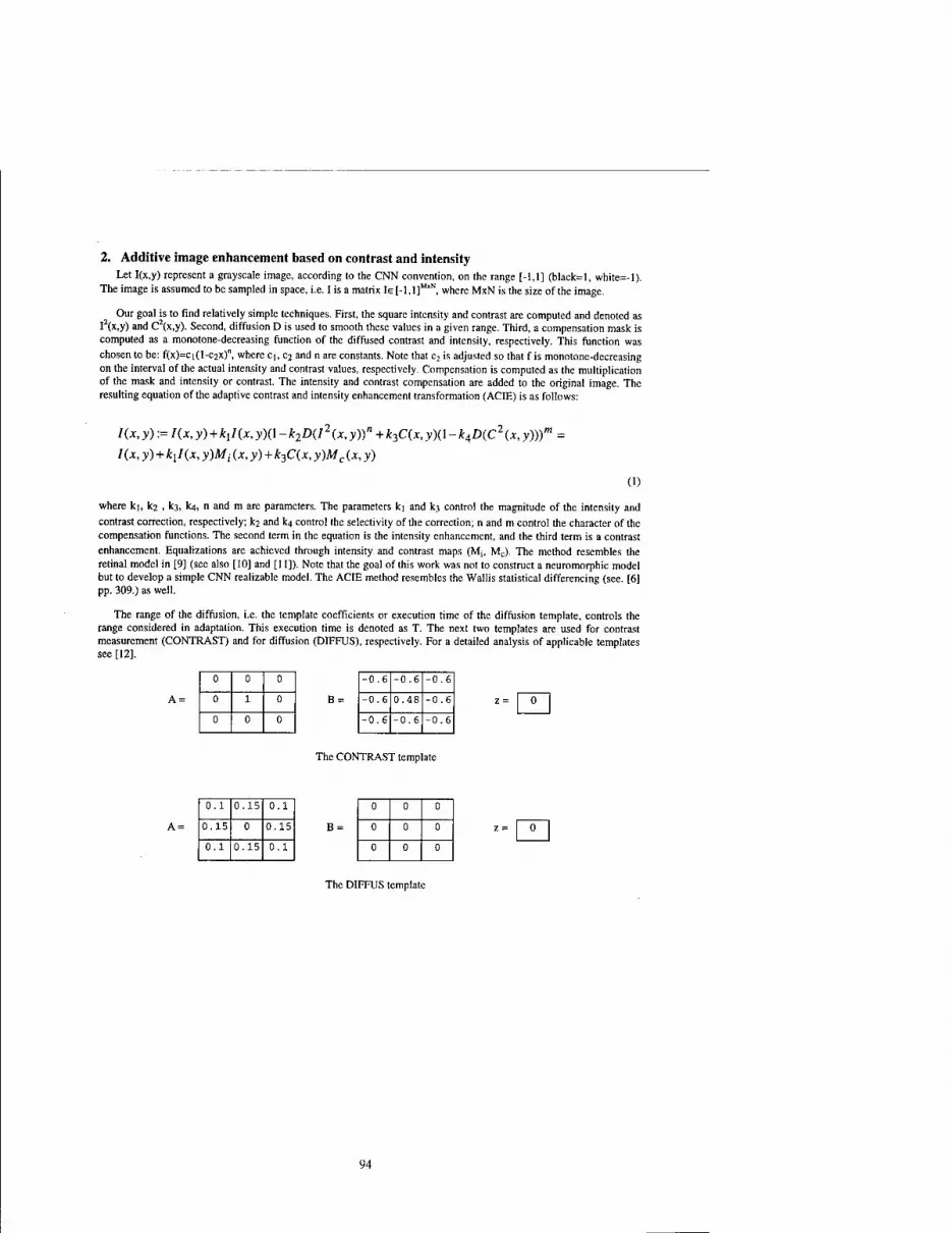
2. Additive image enhancement based on contrast and intensity Let I(x,y) represent a grayscale image, according to the CNN convention, on the range [-1,1] (black=l, white=-l).

The image is assumed to be sampled in space, i.e. I is a matrix Ie [-l,l]HxN, where MxN is the size of the image.

Our goal is to find relatively simple techniques. First, the square intensity and contrast are computed and denoted as I (x,y) and C (x,y). Second, diffusion D is used to smooth these values in a given range. Third, a compensation mask is computed as a monotone-decreasing function of the diffused contrast and intensity, respectively. This function was

chosen to be: f(x)=ci(l-C2X)n, where ci, C2 and n are constants. Note that c2 is adjusted so that f is monotone-decreasing on the interval of the actual intensity and contrast values, respectively. Compensation is computed as the multiplication of the mask and intensity or contrast. The intensity and contrast compensation are added to the original image. The resulting equation of the adaptive contrast and intensity enhancement transformation (ACIE) is as follows:

I(x, y) :=/(*, y) + *,/(*, y)(l - k2D(12(x,y))n + k3C(x, y )(1 - k4D(C2(x, y)))m =

I(x, y) + kxI(x, y)Mt (x, y) + k3C(x, y)Mc (x, y)

(1)

where ki, k2 , kj, lot, n and m are parameters. The parameters ki and k3 control the magnitude of the intensity and

contrast correction, respectively; k2 and lq control the selectivity of the correction; n and m control the character of the compensation functions. The second term in the equation is the intensity enhancement, and the third term is a contrast

enhancement. Equalizations are achieved through intensity and contrast maps (Mj, Mc). The method resembles the retinal model in [9] (see also [10] and [11]). Note that the goal of this work was not to construct a neuromorphic model but to develop a simple CNN realizable model. The ACIE method resembles the Wallis statistical differencing (see. [6] pp. 309.) as well.

The range of the diffusion, i.e. the template coefficients or execution time of the diffusion template, controls the range considered in adaptation. This execution time is denoted as T. The next two templates are used for contrast measurement (CONTRAST) and for diffusion (DIFFUS), respectively. For a detailed analysis of applicable templates see [12],

A =

0 0 0

0 1 0

0 0 0

-0.6 -0.6 -0.6

-0.6 0.48 -0.6

-0.6 -0.6 -0.6

The CONTRAST template

A =

0.1 0.15 0.1

0.15 0 0.15

0.1 0.15 0.1

0 0 0

0 0 0

0 0 0

The DIFFUS template

94

Intensity of row 35 of sensed image

HJ^ Enhanced image and intensity plot in row 35

Sensed Image

Conventional contrast enhancement and intensity plot in row 35

Figure 1 An exponentially decreasing illumination into the right direction is supposed during sensing. Note that the sensed image seems better than it is in reality, because during perception, the adaptive mechanism of the eye of the reader enhances it already, and this process is similar to the technique presented here. The ACIE restores the original image in good quality. The.contrast and intensity of the image are fairly equalized. The conventional contrast enhancement technique oversaturates the contrast at some places (see the border'of the black circle at the bottom left corner) while it does not improve the contrast at other places, moreover, intensity is not equalized (compare the

intensity plots). The parameters of ACIE are: ki=l, ka=2, k3=100, k4=5, T=50TCNN and n=m=3. The equation of the conventional contrast enhancement was I'(x,y)=I(x,y)+3C(x,y).

95

Intensity Compensation

Ä

Figure 2 Outline of flowchart of the ACIE image enhancement algorithm.

3. Adaptive sensing via locally adaptive exposure time Using uniform exposure time, the sensed image may be uneven due to changing illumination. Adaptive sensing

assumes an imaging device with pixelwise programmable exposure time or gain. Adaptive sensing in our case means that the mask of the exposure time Me is programmed adaptively during sensing. This can be achieved by a procedure

described as follows. First, a short enough exposure is taken with uniform exposure, this image is denoted by Io Second, an exposure mask is calculated as:

Me(x, y) := *,/(,(*, y)((l -k2D(I02(x, y)))n + (\-k3D(C2(x, v)))m =

k;I0(x,y)(Mi(x,y) + Mc(x,y))

96

where ki, k2, k3 , n and m are parameters with similar meaning as before. During sensing the intensity and contrast maps are used together as an exposure map. Sensing is modeled with a multiplication with the exposure mask and threshold is also applied:

Is(x,y)=Tr(Io+Io(x,y)Me(x,y))

where Is is the sensed image and the threshold function is Tr(x)=max{-l,min(l,x)}. The exposure mask is computed similarly to the compensation masks in the enhancement method. The result is not as excellent as the output of the adaptive equalization (see Figure 3), since during sensing there is no opportunity for contrast equalization. This method resembles the one used in [7] for estimating light illumination energy for color identification.

Adaptively sensed image and intensity of row 35

r 1A 20 30

Sensed with twice uniform exposure

£: ZO 30 40 BO

Figure 3 Adaptive image sensing equalizes intensity, it is obvious that using uniform exposure the right side will be dim: exponential decreasing tendency in absolute intensity is apparent. The parameters are the same as before for the

contrast and intensity maps: ki=1.5, k2=2, k3=100, k4=5, T=50TCNN, and n=m=3. Note that in reality the left picture is much worse, than it seems to be, because there is an enhancement mechanism in the human visuals system as well.

4. Realization via Adaptive Extended Cell in CNN-UM The method introduced can easily be realized using the Adaptive Extended Cell in CNN-UM ([3]). Time invariant

local control is used via local template memories TCM. The TCM memories are local analog memories associated with the cells, i.e. individual pixels. They are used to control template values. Image enhancement can be implemented by the following template:

A =

0 0 0

Ö I Ö

Ö Ö Ö B =

c c c

c b c

c c c Z =

where c and b are TCM values and they are computed as: c=-0.6Mc(x,y) and b=M;(x,y)+1.48Mj(x,y). The masks are computed as in equation (1) and the acquired image is used as input. Adaptive sensing may be realized by enabling the TCMs to program the exposure time individually for each pixel. This work does not address the possibilities of variable resolution and real time local adaptation, but it is obvious that using our method with real time local adaptation results in a more powerful method.

97

5. Conclusions An adaptive image enhancement and image sensing technique were presented. Both methods use basically the same

technique for equalization as they apply the intensity and contrast information of the basic image. The equalization masks are computed by using the diffusion template via the CNN-UM. The algorithm is ideal for the ACNN-UM The most time consuming task is the diffusion. Accordingly, the use of the currently available CNN-UM chip speeds up the process significantly. On the other hand, the presented methods are of acceptable quality as this is shown by the sample images. In the algorithms the radius of the adaptation can be controlled by the time or gain of diffusion, thus all intermediate cases between full global and local equalization are dynamically available.

6. Acknowledgement The research was supplied by the grant No. T026555 of the National Research Found of Hungary (OTKA) and by

the Hungarian Academy of Sciences.

7. References

[I] L. O. Chua and L. Yang, "Cellular Neural Networks: Theory and Applications", IEEE Transactions on Circuits and Systems, Vol. 35, pp. 1257-1290, 1988.

[2] T. Roska and L. O. Chua, 'The CNN Universal Machine: An Analogic Array Computer", IEEE Transactions on Circuits and Systems-D, Vol. 40, pp. 163-173,1993.

[3] T. Roska, "Analogic CNN computing: Architectural, Implementational and Algorithmic Advances -Review", Proceedings of the CNNA'96, 14-17 April, London, pp. 3-11, 1998.

[4] M. Csapodi, T. Roska , "Adaptive Histogram equalization with cellular neural networks". Proceedings of IEEE International Workshop on Cellular Neural Networks and Their Applications, pp. ,1996.

[5] S. M. Pizer et al., "Adaptive Histogram Equalization and Its Variations", Computer Vision, Graphics and Image Processing, Vol. 39, 3, pp. 355-368, 1987.

[6] W. K. Pratt, "Digital Image Processing", John Wiley & Sons Inc., 1991.

[7] Ä. Zarändy, L. Orzö, E. Grawes, and F. Werblin, "CNN Based Models for Color Vision and Visual Illusions", IEEE Trans, on Circuits and Systems I: Special Issue on Bio-Inspired Processors and Cellular Neural Networks for Vision, (CAS-I Special Issue), Vol. 46, No.2, pp. 229-238, 1999.

[8] H. Zhu, F. H. Y. Chan, and F. K. Lam, "Image Contrast Enhancement by Constrained Local Histogram Equalization", Computer Vision and Image Understanding, Vol. 73, No. 2, pp. 281-290,1999.

[9] S. M. Smirnakis, M. J. Berry, D. K. Warland, W. Bialek and M. Meister, "Adaptation of retinal processing to image contrast and spatial scale" Nature 386, 69-73, 1997.

[10] F. Werblin, A. Jacobs and, J. Teeters, 'The computational eye", IEEE Spektrum, May, pp. 30-37, 1996.

[II] F. Werblin, T. Roska, L. O. Chua, 'The analogic cellular neural network as a bionic eye", Int. Joum. of Circuit Theory and Applications, vol. 23, 541-569, 1995.

[12] K. R. Crounse, "Methods for Image Processing and Pattern Formation in Cellular Neural Networks: Tutorial", IEEE Trans, on Circuits and Systems-I: Fundamental Theory and Applications, vol. 42, no. 10,1995.

98

2000 6™ IEEE International Workshop on Cellular Neural Networks and Their Applications Proceedings

An analogic CNN algorithm for following continuously moving objects

Alexandru Gacsädit, Peter Szolgay

Analogic and Neural Computing Systems Laboratory, Computer and Automation Institute,

Hungarian Academy of Sciences, P.O.B.63, H-1502 Budapest, Hungary, and also affiliated

to Image Processing and Neurocomputing Department, University of Veszprem,

phone: +(361)2095265, fax: +(361)2095264, e-mail: szolgay@srtaki.hu

^University of Oradea, Str. Armatei Romane Nr.5,3700 Oradea, Romania e-mail: agacsadi@el.uoradea.ro

ABSTRACT: A potential application of cellular neural networks (CNN) in adaptive control of a robot based on visual information is considered here. The high processing speed of the network is used to provide real time processing. In this contribution an analogic CNN algorithm for following a moving object is shown. The algorithm was tested with the CNN infrastructure (CADETWin and CCPS).

1. Introduction

An adaptive industrial robot had to have the possibility to perceive the working environment. The visual information on the working area of a robot and the proper control actions are computed even in the presence of inherent errors of the kinematic chain.

The model of a robotic system with image-based command and visual feedback [1] and [2], is presented in Figure 1. In this case, the command is given based directly on the feature detected on the image on feedback way, when reference image has been captured to the system.

Space control

Power amplifiers Robot arm with camera

Reference image + A- Image feature extraction

Figure I: Image-based visual servo structure for robotics system

A simplified model is proposed in Figure 2. The system has a single visual sensor (camera) on the arm of an industrial robot with two degrees of freedom, having just rotation of joints. We select an object from the captured image. Supposing that the position of the appointed object is described only by a single point, by the central point of the object captured by visual sensor, through horizontal coordinate x and vertical coordinate y (see Figure 3). In the image plane of the visual sensor, the central point of the object and the origin of reference system attached to the image plane of the camera are given to angles 61 and 62 of kinematic joint JA and JB. This is to be set manually.

^, ♦ Central point of object (1 pixel)

Image plane of visual sensor with reference

system xOy

selected object

visual sensor

Figure 2: Robotic system having visual feedback Figure 3: The image frame of a camera

Several object selection criterion can be set, for example we can select a single moving object at a given time. The rest of the algorithm will not be changed.

0-7803-6344-2/00/$10.00 ©2000 IEEE 99

The displacement of the selected object has to be decided according to the central point of the object in the reference system. The solution of the kinematic problem of robot arm has to be found.

The speed performance of a CNN-based system will be evaluated [3], [4], [5], [6], [7] and [8]. Thus, starting from acquisition of a current image up to determination of command angles 81 and 62, we want that processing be achieved only in CNN environment in order to increase speed. If the processing speed is fast enough even in the case of position errors, the command will correct the current position before loosing the object.

2. Description of the algorithm

The analogic CNN algorithm of control process image-based visual servo system is presented in Figure 4.

Input binary image

X A. Selection of an object

Follow.tern

I One object image

I B. Determination of

position of central point

Hollow.tern

Center.tem

Cl. Determination of command angles 81

Shsiud.tem

LogAND.tem

Shsirl.tem

Command angles 81

C2. Determination of command angles 82

Shsirl.tem

LogAND.tem

Shsiud.tem

1 Command angles 82

Figure 4: Flow-chart of the algorithm of control process

The main phases of the algorithm are as follows: A. Selection of an object which will be followed through acquisition of an image. It is desired to bring the

central point of the object in the origin of reference system attached to the image plane as close as possible at the time t0 = 0. The input images will be sampled with time step T. After that image sequences must be processed so that only the selected object remains in the output image in the current position. We suppose that objects are separated in the input image. Otherwise the analogic CNN algorithm will combine the overlapping

100

objects into a single one. A mask image containing only the appointed object is created. The intersection of this mask and the moving object must not be empty. The mask image is the output of the previous stage.

The "follow.tem " has been used with the input image on INPUT and the mask is STATE of the CNN. Follow.tem

A =

0.275 0.275 0.275

0.275 2.300 0.275

0.275 0.275 0.275

0 0 0

0 3 0

0 0 0

The number of iterations depends on the character of the input image, dimensions of the appointed object and difference between two successive positions of the appointed object.

The difference between the selected objects in two consecutive images can be several pixels in the direction of motion. To have a correct result it is sufficient that at least one common element exists between two successive positions. Having time step T and a N*N pixel object to follow, the maximal speed that we can catch up with is N/T pixels/second in a certain direction. If an other object overlaps a marked object it is possible that the other object will be followed. In this case a new selection is necessary.

B. Determination of the position of the central point of the selected object from image, through coordinates from image plane, x and y. A sequence of templates has been used to peel the object from different directions until the object has only one point and its coordinates are those of the object.

The peeling (erosion) is symmetric because it is applied in each direction N, S, E, W, N-W, N-W, S-E, S-W. But if it is applied with a different number of iterations for different directions, it can result a point which is not the accurate central point of an object [9].

Until now it has been supposed that the object which has been peeling is of a closed contour formed by black (+1) pixels. But if the appointed object has no closed contour ( due to bad illumination) the method does not give the correct results. According to some experimental results of preprocessing with the hollow.tem template [9] the results have been promising.

C. Determination of angles 91 and 02, which will constitute the command angles to position robotic arm. This means solving the inverse kinematics problem, that is determination of coordinates in joints reference systems, JA and JB. Each of these stages will be achieved in a few processing steps.

A three-layer CNN structure has been used to solve this problem (see Figure 5). s-

x ^*

7 Layer1

Image plane of Camera P(x,y,kT)

Layer 2 Image angle 81

04- Command angle 81(kT)

V j_ i s Layer 3

Image angle 92

°^^ y A-- Command angle 92(kT)

■>' MUM

Figure 5: Structure of neural network attached to command of system

Layer 1 does the acquisition of the current input image and after some elementary processing steps, it will result an image containing only one active pixel with value +1. By following the position of this pixel, it will result the coordinates of the object in the image plane, x and y. Layer 2 and 3 will be controlled by this layer.

Layer 2 is associated with the command image 81, it is to obtain the command angle corresponding to 81 at each horizontal position derived from layer 1.

Layer 3 is associated with the command image 82, it is to obtain the command angle corresponding to 82, after it has been derived from the vertical coordinate in the image plane. We consider that layer 2 and 3 are necessary to solve the inverse kinematics problem.

The images of the command angles 81 and 82 could be computed in three different ways: (i) Gray scale images can be used, where each pixel contains the information concerning command angles 91

and 82, in the given layer (see Figure 6 a). In this case there is no approximation but it requires a longer processing time to determine the command angles, mainly due to the process of central point determination.

(ii) Using gray scale images containing identical pixels on a column (81), and a row (82), if angle 81 is in joint system, it is independent of the vertical position of the object and if angle 82 is in joint system, it is independent of the horizontal position of the object. Each pixel containing (through its gray level) the

101

information regarding 81 and 82 (see Figure 6 b). In this case the approximation allows for the image to become even binary, so that each column (Gl) and each row (62) contains the information (binary coded) regarding to the reference angles. This method has been used in our example(see Figure 6 c).

(iii) Binary images for the simplest situation when the images of the command angles (81 and 82) serve only to determine the variation of these angles referring to current position (A6>0 or A8 <0, see Figure 6 d). In this case the computation of the hollow.tem and the central point of the moving object can be skipped .

(b) (c) Figiire6: Examples for images angles 6

The selection criterions of the method describing the operation of 61 and 62 layers are as follows: (i) The accuracy of the computation. (ii) The type of the CNN-UM chip which is available in the implementation of the algorithm.

Having the coordinates of the marked object, the values of the angles of the next position, 81 and 82, have to be determined on layer 2 and layer 3, respectively.

To determine 61 of the center point of the object to be followed, a shadow (N-S, North-South) has been used ("Shsiud.tem") [9]. The command angle 81 of the current position is determined by the AND function of the previous step and the image 81. To read the results from the same place, a shadow (E-W) has been used, ("Shsirl.tem") [9], The analog value of the command angle of joint JA will always be in the rightmost column of the image. When determining 82, a row of image 82 will be selected, controlling the vertical position of active pixel from layer 1.

Between two consecutive images, all the processing for a current input image has to be carried out, in order not to loose the object. Thus following of an object will be considered as a continuous one, even if the principle uses images sampled (in time) with step T.

3. The experimental system and an example running onCADETWin

The experimental system using CADETWin (CNN Application Development Environment and Toolkit under Windows) [10] is presented in Figure 7.

Multi - Layer CNN Simulator (SimCNN)

running on a Pentium chip < ►

PC Pentium with CADETWin CNN Chip Prototyping

System (CCPS) with CNN-UM

Figure 7: The experimental system

3.1 Simulation example

The Analogic CNN algorithm was tested by using "SimCNN - Multi - Layer CNN Simulator with the Visual Mouse Platform [11] and CNN Chip Prototyping System (CCPS) with CNN-UM" [12]. Though in this paragraph a software simulator was used but keeping in mind the capabilities of the analog 20*22 CNN-UM chip with direct optical input [13].

The critical steps of the object following analogic CNN algorithm are shown in Figure 7.

102

'A' ja. Ja)

N/1 (c) A

(e) (f)

/ 1 \

(g)

■ ■

(h)

(i) (j) (k) (1) Figure 7: Simulation of analogical algorithm for CNN processing of an input image: a) INPUT actual image, b) OUTPUT after Follow, c) OUTPUT after Hollow, d) OUTPUT actual position, e) OUTPUT after Shiiud,

filmage 61, g)OUTPUT after AND, hJOUTPUT after Shsirl, i) OUTPUT after Shsirl, jjlmage 82, k)OUTPUT after AND, l)OUTPUT after Shsiud

3.2 The analog CNN Universal Machine implementation

There is some chip limitation in the case of Universal Machine implementation [12] and [13] of analogical CNN algorithm for continuously following an object. The most important points are as follows:

(i) Maximum number of images which can be loaded on circuit at a moment, (ii) Maximum number of templates which can be used.

Template Sim CNN (xl) 20*22 CNN-UM (x)

Acquisition - ~1 Follow.tem <50 40 Center.tem 72 72 Hollow.tem <40 50 Shsiud.tem <22 <22

LogAND.tem 1 1 Shsirl.tem <22 <22 Shsirl.tem <22 <22

LogAND.tem 1 1 Shsiud.tem <22 <22

Total <252 <253 Tablel: Running time estimation of the analogic CNN algorithm (measured in time steps)

On the other hand, some of the templates need a 'fine tuning" to give the same results as we had by the software simulator.

Processing time of the algorithm implemented by Sim CNN software simulator and by 20*22 CNN-UM are presented in Table 1. The processing time at most of the templates used in this analogic CNN algorithm were proportional to the object size to be followed.

103

In our experiences, the 20*22 CNNUM chip was used with a time constant x=250 ns. The algorithm of following moving object results 63.25 p.s total time processing.

4. Conclusions

An analogic CNN algorithm was developed to follow moving objects. The algorithm was tested in CADETWin simulation environment and on 20*22 CNNUM chip with CCPS.

The analysis of the described robotic system shows that our analogic CNN algorithm provides a proper solution to the problem.

In the near future the algorithm will also be tested by 64*64 CNNUM chip [14] with CCPS, providing a higher computing speed, gray-scale direct optical input and fixed state map options.

5. Acknowledgments

The authors are thankful for the helpful discussion with Professor Tamas Roska.

6. References [I] S. Hutchinson, G. D. Hager, P.I. Corke: "A Tutorial on Visual Servo Control", IEEE Trans. Robotics and Automation, Vol. 12, pp. 651-670, Oct. 1996. [2] W. J. Wilson, C. C. Williams Hulls, G. S. Bell: 'Relative End- Effector Control Using Cartesian Position Based Visual Servoing" IEEE Trans. Robotics and Automation, Vol. 12, pp. 684-696, Oct, 1996. [3] L. O. Chua, L.Yang: 'Cellular neural networks: Theory", IEEE Trans. Circ. Syst. Vol. 35, pp. 1257-1272, Oct. 1988. [4] L. O. Chua, L.Yang: 'Cellular neural networks: Applications", IEEE Trans. Circ. Syst.-I, Vol. 35, pp. 1273- 1290, Oct. 1988. [5] L. O. Chua, T. Roska: "The CNN paradigm", IEEE, Trans. Circ. Syst. Vol. 40, pp. 147-156, March 1993. [6] T. Roska, L. O. Chua: "The CNN Universal Machine an analogic array computer", IEEE Trans. Circ. Syst., -II Vol. 40, pp. 163-173, March 1993. [7] P. Szolgay, A. Katona, A. Kiss, L. Szekely, A. Veress: "An optical robot path tracking system", Toward the Visual Microprocessor- VLSI Design and Use of Cellular Network Universale Machines (Toward the Visual Microprocessor), T. Roska and A. Rodriquez-Vazguez, J Wiley, 1997. [8] B. Siemiatkowska: 'Cellular Neural Network for Mobile Robot Navigation", CNNA-94, Proc. IEEE International Workshop on Cellular Neural Networks and their Applications, pp. 285-290, Dec, Rome 1994. [9] T. Roska, L. Kek, L Nemes, A. Zarandy, M. Brendel, P.Szolgay: 'CSL - CNN Software Library (Templates and Algorithms)", Users Guide, Version 7.2 Analogical and Neural Computing Laboratory, Computer and Automation Institute of the Hungarian Academy of Sciences, Budapest, 1998. [10] CadetWin99 CNN Application Development Environment and Toolkit under Windows Users Guide, Analogical and Neural; Computing Laboratory, Computer and Automation Institute of the Hungarian Academy of Sciences, Budapest, 1999. [II] I. Szarmari, L. Kek, Cs. Rekeczky, T. Roska: "SimCNN - Multi - Layer CNN Simulator for the Visual Mouse Platform", Users Guide, Version 2.0, Analogical and Neural; Computing Laboratory, Computer and Automation Institute of the Hungarian Academy of Sciences, Budapest, 1997. [12] P. Földesy, T. Roska, P.Szolgay, A. Zarändy, S. Zöld: 'CCPS97-Alpha Language and Compiler in the CCPS System", Users Guide, Version 1.1, Analogical and Neural Computing Laboratory, Computer and Automation Institute of the Hungarian Academy of Sciences, Budapest, 1997. [13] S. Espejo, A. Rodriguez-Vazguez, R. A. Carmona, P. Földesy, A. Zarändy, P.Szolgay, T. Sziränyi, T. Roska: '0.8 u.m CMOS Two -Dimensional Programmable Mixed - Signal Focal - Plane Array Processor with On - Chip Binary Imaging and Instructions Storage", IEEE Journal of Solid - State Circuits, Vol. 32, No.7, pp. 1013-1026, July,1997. [14] G. Linan, S. Espejo, R. Dominguez/Castro, E. Roca, A. Rodriguez-Vazquez,:" CNNUM3: A mixed-signal 64x64 CNN Universal Chip", Proc. of MicroNeuro99, pp. 61-68, Granada, 1999.

104

2000 6™ IEEE International Workshop on Cellular Neural Networks and Their Applications Proceedings

Collision Prediction via the CNN Universal Machine

V. Gäl and T. Roska

Analogical & Neural Computing Systems Laboratory at the Computer and

Automation Research Institute of the Hungarian Academy of Sciences

H-llll Budapest Kendeu. 13-17, Hungary

ABSTRACT: In this paper we present an analogic CNN algorithm that estimates the time to an impending collision between an approaching object and the observer. Calculation is based on a context insensitive method, which is well known in neurobiology, using only two specific cues of the expanding two-dimensional image of the looming object.

1. Introduction

Predicting dangerous or advantageous situations has similar importance for animals and for machines. One of these situations is when the motion of an object could end up with a useful (for a predator) or disadvantageous (for a prey) collision with the observer. A growing body of evidence makes neurobiologists suppose that for some animals (and humans) low-level visual information alone is enough for a remarkable estimation of the time left till an impending collision.[l],[2] Fast calculation even in an unfamiliar environment may have a life-saving impact. According to recent theories, calculation can be based upon only two optical variables of looming objects, ensuring the relative context-insensitivity of the process.[3],[4] Precise information about the size (diameter) of the two-dimensional projection of the object and the rate of its expansion are enough to predict the so called time-to-collision(TTC), provided that the motion is at a constant speed.

The type and simplicity of the method allow for the development of CNN algorithms [5] for the problem of collision prediction. Our analogical algorithm consists of 3 by 3 linear templates and has no special CNN architecture requirements, so it can be implemented on existing visual microprocessors.[6],[7]

2. Estimating the 'Time-to-Collision' (TTC): Optical Geometry

A method, which is supposed to be used by the neural system of some animals for TTC estimation could be derived from the following equation:

TTC = —^—, (1)

where d is the diameter and v„,ge is the velocity of the edge of the expanding image (Fig. 1.). As the object approaches, the increase in the relative rate of expansion is higher than that in the diameter.

There is a law well known in optical geometry (the notations in the equations below are defined in Figure 1.):

'(.'left) _ D

f d('left) (2)

and we can write:

s(<left) = vtleft (3)

-T d ('left) = vedge.up ~ vedge.down (4)

0-7803-6344-2/00/$10.00 ©2000 IEEE 105

where — d is the rate at which the diameter expands. From equation (2), (3): at

dt K"fi' dt JD

*(V> =p dt vt,

10.

= fl> K,)2 (5)

The TTC, according to the definition above (1), and from (2), (3), (4) and (5) is:

(6)

so the ratio between the diameter and the rate of its expansion is equal to the time left to a direct collision.

plane

Vedge.up(tlefl)

d(tleft)

v edge.down\Uefi) ^^ rr

S(tleft)

Figure I: An object approaching the observer's eye (or detector). tUß, time left to collision; D, diameter of the object; v, velocity of the object; s(tirj<), distance between the observer and the object; d(ti,fl), diameter of the projecting image at the focal-plane; f, focal length; vrf/,,„/r,,„) and v,JgrdmJtirß), speeds of two opposite edges of the image, parallel to the focus plane.

2. The Analogic Algorithm on the CNN-UM

The principles of the TTC calculation explained could help in the development of an analogic CNN algorithm that can alarm an observer-machine a certain time before an impending collision.

First, we assume that an appropriate detector captures subsequent images (frames) of a looming object at a constant sampling rate. The images are forwarded towards a computer with standard CNN-UM architecture, which processes the following steps. After some transformations (described thoroughly in Figure 2. and 3.), the optical variables of the image of the object will be represented by the darkness of an image: the length of the diameter and the extent of the expansion will be encoded by the value of the pixels (cells) in the picture (array).(Figure 2. n, Figure 3,j)

For example, if the horizontal diameter is 4 pixels long (Fig. 2.a), then—after a few operations (figure 2.b- 1)—the state of the cells in the 4,h row (numbered from the reference line (Figure 2.1), which is the upper side of the frame in this case) will be set to +1 and the rest to a negative number.(Figure 2.1) Its inverted form will serve as a fixed state mask on a special grayscale image at the next step. (Fig. 2.m) This image consists of rows with different colours. The values of the pixels belonging to one column are equal, but there is a graded, logarithmic change from one column to the next. In a kxl array, the value of a P pixel in the z" column and the n"1 row is defined by the expression below:

Pn,z=i°ei "

106

Fixing the state of the cells belonging to the 4th column (in this example) we apply a massive diffusion. (Figure 2.m,n) The result is a homogenous picture whose pixels have the same value; moreover, it is equal to the 4"1 column's original value (in the previous picture). Thus, the length of the diameter is represented by the value of the pixels of a picture. (Figure 2.n)

a) Object in the N* frame

1 r b) FILLROW

Fills the occupied rows

> 1 rc) LEFTEDGE ^

Clears everything except ^ the left side ^

1 r d) TRIANGLER1GHT

Creates a (45°, 90°, 45°) triangle, using the previous

line as the hypotenuse

ac e)TRIANGLERIGHT

-EDGE Clears everything except

the inner peak „

^ f) FILLROW Fills the selected (occupied)

rows

I f g) f AND a i

Extracts the horizontal diameter of the original

object: logic AND between the original image (a) and f.

Reference line

4"tow

h) FILLCOLUMN ^ Fills the selected (occupied)

. columns.

I i) UPPEREDGE

Clears everything except the upper side

j) TRIAGLE2DOWN Creates a triangle starting

from the line in the previous picture, leg A=leg B

k) FILLROW Fills the occupied rows

1) BOTTOMEDGE Clears everything except the

bottom row

I rm) NOT(l)

Masking the special grayscale image with the

invert of the previous image

n) DIFFUSION Applies massive diffusion

Figure 2. Steps of encoding the size. The length of the diameter of an approaching object's image is represented by the darkness of a grayscale picture after the final step. The names of the templates are in capitals. Black pixels in the pictures represent the results of the current template-operations superimposed on the results of the previous operations (gray pixels). Picture m and n are exceptions, where the colours have special meanings described in the text.

The speed of the approaching is reflected in the rate of change in the image size. Higher speed resulted in more pronounced difference between two subsequent frames in regard to the dimensions of the image of the looming object. The change in the diameter can be represented in a very similar way as the length of it (as described above). If its size grows by two pixels from one frame to the next, the value of the pixels in the second column will be set to +1 and the rest are -1, as a result of subsequent template operations (Figure 3.a-h). Following steps (masking, diffusion) are the same as in the description above (Figure 3.i,j).

107

The final step (Figure 3.1) is the subtraction of the grayscale image which we got at the end of the analysis of the motion (Figure 3.j) from the image we obtained after size-analysis (Fig. 3.k and Fig. 2.n). Since the pixel value represents logarithmic transformations of size and edge-velocity, the result of the subtraction encodes the ratio between these two optical variables. This ratio is a very useful parameter that can determine the TTC directly as we have explained above (see equation (6)).

a) The approaching object in the N"1 frame

and its horizontal diameter

b) The approaching object in the (N-l)* frame

and its horizontal diameter )

c) Creating a band with a width equal to the diameter. Algorithm is described in

i Figure 2.a-k

e) NOT(d)ANDc Extracting the change

between two subsequent frames (c and d). s (c ai

f) LEFTEDGE Cleares everything except

the left side.

r g)TRIANGLERIGHT ^ and T. RIGHT-EDGE

Creates a triangle starting from the extracted line and i finds thejnper peak, j

r h) FILLCOLUMN Fills the selected (occupied) . column.

I sp Masking the

special grayscale image with the invert of the

previous image

i) DIFFUSION Applies diffusion

I

fjinn^^— <....;

öfte

r.

■ = =<

d) Creating a band with a width equal to the diameter. Algorithm is described in

i Figure 2.a-k

k) Transforming the width of the band into a homogenous grayscale image by the method

described in Figure 2.k-n

1) M Subtracting the

homogenous grayscale image representing the motion from the image

encoding the size

Figure 3. Steps of encoding the rate of the expansion. The change in the length of the diameter of an approaching object's image is represented by the darkness of a grayscale picture.

108

To illustrate the calculation, we take 64X64 sized frames with a 10/sec frame-rate. In the n* frame, the diameter of the projecting image is 30 pixels, while in the (n-1)"1 it is 26 pixels. The speed of the image's edges is 4 pixels/frame, which means 4 pixels/0,1 sec. The result of the analogic process—the value of the pixels in the picture generated by subtraction at the end—(from equation [6]) is:

log64 30 - log64 4 = log« ^ = 0.4844 4

This means that there is 0.749sec left before the collision because:

TTC = diameterjvtdge

l°g64 diameter

vedge = l°g64

30pixels

ipixels/OAsec -- l°g64 30pixels 1

4 pixels/sec 10 = l°g64 30pixels

4pixels/sec -Iog64(l0sec)

l°g64 diameter

vedge = log64

30 - Iog64(l0sec) = 0.4844 - 0.5536 = -O.0692

l°g64 TTC = 64

diameter vedge = 64~°-0692=0,7499sec

FillRow FillCol

Propagating templates: they fill those rows/columns in which at least one black pixel occurs.(Figure 2.b,f,i,k; Figure 3. H)

LeftEdge UpperEdge RightEdge BottomEdge

Uncoupled templates: they find the left/upper/right/bottom line of a rectangle, and clear the rest of the object.(Figure 2.c, i, 1, Figure 3.f,g)

TriangleRightEdge Uncoupled template: it finds the right peak of a triangle and clears the rest of the object.(Figure 2.e)

Triangle2Right Tiangle2Down

Propagating templates: they create a (45°, 90°, 45°) triangle starting from a given line (it will be the base of the triangle) at the left/upper side of the frame, whose height is equal to its base. (Figure 2.j, Figure 3.g)

TriangleRight Propagating template: creates a (45°, 90°, 45°) triangle starting from a given line (it will be the hypotenuse of the triangle) at the left side of the frame, whose height is the half of its hypotenuse.(Figure 2.d)

Diffusion Propagating template. Its function is a massive diffusion on a grayscale image, where the state of the cells in a preselected row/column is fixed. The result is a homogenous grayscale picture.(Figure 2.n; Figure 3.j)

Table 1: Short description of the templates used by the algorithm.

3. Simulation Results

We simulated a collision with two different sets of parameters (Table 2.) on a 64 by 64 sized simulated CNN- UM at 33/sec frame rate. In both cases, we set the threshold level (the program has to warn the observer tte„hoid before the collision) to 195msecs before the impending collision. The accuracy of the estimation of the TTC by

109

the algorithm was in the range of the frame rate (which means 30 ms between two frames). When the threshold was exceeded, calculated TTC (by the analogic algorithm) was 192msecs and simulated time to collision was 180msecs in both cases. In the case of the smaller and faster object, the algorithm alarmed the 'observer' when the distance was 720cm from the detector and the size of its image was smaller than in the case of the bigger and slower object.

Parameter Objectl Object2

Speed 40m/sec (144km/h) 30m/sec (108km/h)

Size (diameter) 15cm 21cm

Simulated time-to-collision 180msecs 180msecs

Calculated TTC 192msecs 192msecs

Distance from the observer at simulated time-to-collision

7.2m 5.4m

Table 2. The parameters of the simulations. The table shows the simulated time and calculated TTC at the moment of warning of the analogic program.

4. Conclusion

Based on a neuromorphic model the 'time-to-collision' parameter has been computed via a simulated CNN Universal Machine using the described algorithm. Basically, the accuracy of estimation depends on the size of the array of the CNN cells (resolution) and the sampling-rate (frame-rate) at which the CNN-UM can process the calculation. Provided that the speed of the calculation enables processing at 33 frame/sees (30msec between two frames) and the program is running on a 64 by 64 sized chip, the TTC before collision with an object approaching at 144km/h can be estimated with high accuracy in the last 200msecs. The characteristics of the real 64X64 CNN-UM (according to the measurements performed in our laboratory) enable the process between two frames to be completed in 27msecs. Using a higher speed throughput (40 MS/sec) the processing time will dominate and will allow computation at 400 frame/sec.

Acknowledgments

The support of the Neurobiology Unit of the Hungarian Academy of Sciences at the Semmelweis University of Medicine, the Computer and Automation Research Institute as well as the OTKA grant T026555 are gratefully acknowledged.

4. References

[1] F.C. Rind and P.J. Simmons: "Seeing what is coming: building collision-sensitive neurones", Trends in Neuroscience, Vol. 22, pp. 215-220, 1999. [2J W. Schiff and M.L. Detwiler: "Information used in judging impending collision.", Perception, Vol.8, pp. 647- 658, 1979. [3] H. Sun and B.J. Frost: "Computation of different optical variables of looming objects in pigeon nucleus rotundus neurons", Nature Neuroscience Vol. 1, pp. 296-303, August 1998. [4] G. Laurent and F. Gabbiani: "Collision-avoidance: nature's many solutions" Nature Neuroscience, Vol.1, pp. 261-263, August 1998. [5] B. Shi: "Second order CNN Arrays for Estimation of Time-to-Contact", in Proc. CNNA-96, pp. 427-432., June 1996, Seville, Spain. [6] T. Roska and L.O. Chua: "The CNN universal machine: an analogic array computer", IEEE Trans, on Circuits and Systems II: Analog and Digital Signal Processing, (CAS-II), Vol.40, No. 3, pp. 163-173, 1993. [7] Ä. Rodriguez-Vazquez, S. Espejo, R. Dominguez-Castro, and G. Linan: "The 64x64 Analog Input CNN Universal Machine Chip and its ARAM", Proceedings of International Symposium on Nonlinear Theory and Applications, (NOLTA'98), pp. 667-670, Le Regent, Switzerland, 2-88074-391-5, 1998.

110

2000 6™ IEEE International Workshop on Cellular Neural Networks and Their Applications Proceedings

Optimal CNN templates for deconvolution

Läszlö Orzö

Analogical & Neural Computing Systems Laboratory at the Computer and Automation Research Institute of the Hungarian Academy of Sciences

H-l 111 Budapest Kende u. 13-17, Hungary Phone-Fax: 36-1-209 5357. E-mail: ORZO@LUTRA.SZTAKI.HU

ABSTRACT: A simplified version of the gradient descent method is introduced as a straightforward way to find optimal 3x3 CNN templates for the inversion of known point spread functions (PSF). In practical applications the determination of this inverse is necessary to fulfil deconvolution tasks. The proposed method is much faster than the previously applied algorithms (like genetic algorithm) and still, in almost all practically important cases, it is convergent Moreover, unlike a closed form method [1], it leads to 3x3 templates instead of 5x5 or bigger ones. In several important practical cases the PSF, which can be caused by motion, out of focus or the aberration of the imaging system, can be computed from object positions and from the optical system's parameters. Iterative deconvolution algorithms, which are necessary for volume reconstruction from microscopic image sequences, require considerable computation time. Using CNN-UM chips for these deconvolution tasks, a much higher speed, even real time processing seems to be achievable.

1. Introduction It has previously been confirmed that the CNN is a highly efficient frame for deconvolution and deblurring tasks

[1-6]. CNNs perform spatial filtering by using both feedforward and feedback templates [7-8]. These properties provide the potentiality to implement a wide class of IIR and FIR filtering [9], The main problem lies usually in the determination of the optimal template parameters that can fulfil the above mentioned tasks [9]. Previously there were attempts to determine the template values by using genetic algorithm [10-11]. Our goal in this paper is to show that a simplified form of the CNN [12] gradient descent algorithm examined recently (further references can be found within the cited article) can be applied. Our method provides a favorable framework for the determination of the optimal template elements.

The PSF is generally unknown, but in some important cases it can be determined from the parameters of the imaging system or can be measured. There available freely software packages on the WWW to help compute the PSFs from the object position and from the microscope's optical parameters. Thus in several important applications it can be assumed that the PSF is known.

2. Method A restricted form of the gradient descent algorithm was first introduced [13-15] for B template learning. It was

applied to optimize the performance of the CNN templates on actual, individual chips. The simultaneous determination of the A and B templates is a more complicated problem. It was lately examined [12] and tested for several tasks. Here we consider a simplified version of this detailed [12] gradient based CNN template learning algorithm. This constrained algorithm examines those CNN templates, which employ only the linear part of the operation range and nothing but the static, equilibrium states are taken into account. The effects of these CNN templates can be regarded as a spatially filtered version of the input. These are important simplifications on the otherwise complex algorithms. Thus the reduced method can not handle those problems in which active propagation occurs or a considerable part of the CNN cells is driven into the nonlinear range. This algorithm does not ensure exact inversion of the PSF, but it can find optimal inverse A and B templates in a root mean error sense. If the inverse exists then these templates or a series of them can successfully approximate it.

As the dynamics of the CNN is determined only by a few parameters (overall 19 parameters can describe the 3x3 A and B templates and the bias term.), the gradient descent algorithm does expectedly not stuck in any local minimum. However, this is usually not the case when nonlinear and propagating templates are considered as well [12]. The PSFs, as convolution kernels, can be regarded as big B templates in the CNN terminology.

In the following, we shall use matrix and vector notation for the applied CNN operations.

0-7803-6344-2/00/$10.00 ©2000 IEEE 111

First we have to find the W matrix, which minimizes the mean square error term (E ). It can be found with the gradient descent algorithm.

y = BPSFU

2 2 E = (Wy -u) = minimal

dE*

dW

AW <

= 2(Wy - u)y = 2Ey

dW

(1)

Where u is the input, y is the blurred image degraded by the PSF (BPSF).

As we try to find the inverse as an approximation of the CNN templates, we are looking for W in the next form:

1, W=(!-A) B

Where A and B according to the A and B templates defined hyper-matrices and / denotes the identity matrix. This can be done because we are looking for the CNN's equilibrium solution in the linear range (see above):

u' = Au'+By

u'={I-A)~1By

u' denotes the reconstructed input, so we can define the partial derivatives in the A and B template elements' direction.

(2)

(3)

dB

dE dW

dW dB = 2E((I -A) -\)

3^

dA

dE dW

dW dA = 2f(7- Af E)((I- -Af ]By) (4)

AB = -f,((I-A) lBy-u)((I-A) ly)

AA-- -M((I-A) \{I-A) XBy-u))((l-A) XBy)

\l parameter determines the learning rate. All of these operations can be accomplished within the CNN framework. For known y and u original images this method provides a batch algorithm which assures considerably fast convergence. Only the pixel-wise multiplication and the averaging over the whole images are those operations, which can not be solved easily on the existing CNN chips [16). These operation, however, are still integral parts of the CNN paradigm [8]. Hopefully, the future version of the CNN chips will handle these tasks much better.

3. Results

To demonstrate the effectiveness of this paradigm we carried out simple tests. The applied test PSF kernel is given in the next 7x7 template:

0.0002 0.0008 0.0011 0.0016 0.0010 0.0007 O.OOOll

0.0018 0.0115 0.0217 0.0267 0.0202 0.0096 0.0010

0.0049 0.0478 0.1453 0.1605 0.1327 0.0356 0.0032

0.0051 0.0628 0.2771 0.4875 0.2381 0.0585 0.0052 (5)

0.0021 0.0292 0.1264 0.2116 0.1833 0.0490 0.0048

0.0002 0.0043 0.0217 0.O382 0.0363 0.0196 0.0024

0.0000 0.0002 0.0012 0.0025 0.0025 0.0016 0.0006

PSF

112

It is importante to note that real PSFs are usually non-negative. Nonetheless, we have tested big B templates with some negative entries as well.

This template is invertible as it is the convolution of three different, invertible 3x3 templates. The resulting template or convolution kernel is evidently not symmetric.

The next figure (Figure 1) demonstrates the result of the template learning algorithm after 50 steps of iteration. Within each iteration step we used 32x32 pseudo random images, but the algorithm works for almost any type of image training sets as well.

m i^yxM

:1^$*§& ^fe ? ^ IS.* '4 ;%

Figure 1. We can compare the effects of the deconvolution (C) to the original image (A) and to the degraded image (B). The D, E and F insets are the zoomed regions of A, B and C respectively.

The resulting A and B templates were the following:

113

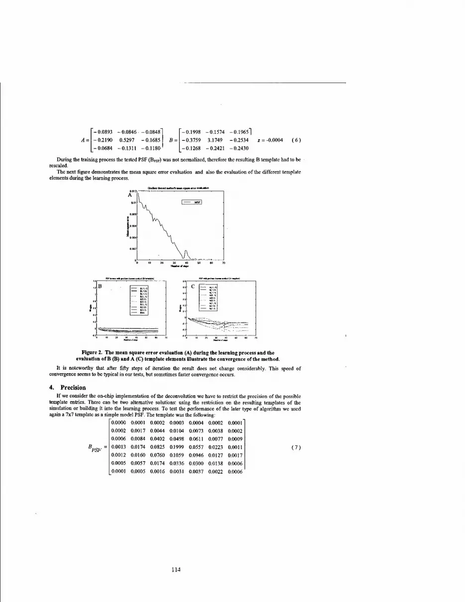
-0.0893 -0.0846 -0.0848

-0.2190 0.5297 -0.1685

- 0.0684 -0.1311 -0.1180

-0.1998 -0.1574 -0.19651

-0.3759 3.1749 -0.2534

-0.1268 -0.2421 -0.2430

z = -0.0004 ( 6 )

During the training process the tested PSF (BPSp) was not normalized, therefore the resulting B template had to be rescaled.

The next figure demonstrates the mean square error evaluation and also the evaluation of the different template elements during the learning process.

kw.rtp.IMI UVHM (B lanvMa) I.I

B tj B(-1-1| B(-lfl)

ei-1.1)

»•• B(l,.1)

B(l.0)

eu>

" —* »jWriBtl1.1.- -*r-

PSP^tp.Jwl. ■M.I -JtAi—»*»)

in <: *t-'."l

»(0.-1)

»(0.11

r — Hi*

^=5JKs£C—-"".

~"--i.-- ^-*>

Figure 2. The mean square error evaluation (A) during the learning process and the evaluation of B (B) and A (C) template elements Illustrate the convergence of the method.

It is noteworthy that after fifty steps of iteration the result does not change considerably. This speed of convergence seems to be typical in our tests, but sometimes faster convergence occurs.

4. Precision If we consider the on-chip implementation of the deconvolution we have to restrict the precision of the possible

template entries. There can be two alternative solutions: using the restriction on the resulting templates of the simulation or building it into the learning process. To test the performance of the later type of algorithm we used again a 7x7 template as a simple model PSF. The template was the following:

0.0000 0.0001 0.0002 0.0003

0.0104

0.0498

B = 0.0013 0.0174 0.0825 0.1999 0.0557 0.0223 0.0011 (7)

0.1059

0.0336

0.0031

PSF

0.0002 0.0017 0.0044

0.0006 0.0084 0.0402

0.0013 0.0174 0.0825

0.0012 0.0160 0.0760

0.0005 0.0057 0.0174

0.0001 0.0005 0.0016

0.0073 0.0038 0.0002

0.0611 0.0077 0.0009

0.0557 0.0223 0.0011

0.0946 0.0127 0.0017

0.0300 0.0138 0.0006

0.0037 0.0022 0.0006

114

The trained A and B templates were the following:

- 0.023 0.000 - 0.070 -0.093 -0.187 -0.375

-0.164 0.421 -0.023 B = - 0.468 3.468 -0.187

-0.046 -0.117 -0.187 -0.187 -0.468 -0.375

z = -0.023 (8)

As it can be seen the minimal step of the template entries was 3/128, that is 0.023. (The PSF was not normalized during the training, therefore the B template had to be rescaled) The results of this learning can be seen in the next figure.

Figure 3. We can compare the results of the PSF (B) on the original image (A) and the efficiency of the reconstruction (C).

This approximation is not as precise as it was in the non-restricted model but it still provides a relatively fair solution.

5. Discussion We were able to demonstrate that even big neighborhood PSFs can be successfully inverted by simple 3x3 CNN

templates. The precision of the original image reconstruction is convincing. Our results further corroborate the strength and potency of the CNN paradigm.

The satisfactory performance of the algorithm encourages us to utilize this method in different applications. What kind of application can it be? There are many image processing algorithms which use deconvolutions for microscopic image's iterative volume reconstruction. These methods remove the out of focus blur [6,10,11] from the images. However, due to their iterative nature these methods are computationally expensive and so they are very time consuming. Hopefully, they can be considerably accelerated by appropriate CNN hardware. Another possible utilization of this method can be a new type of spatial filter design [9] technique. If the spatial filtering characteristic is given in the frequency space, the appropriate convolution kernel can be determined by inverse Fourier transformation. There are further constraints to get real templates. The resulting convolution kernel, however, will

115

not be restricted to the 3x3 size in general. Our simplified algorithm can find the optimal CNN templates in this case as well. Expectantly, the fast convergence of the algorithm can be used in different blind deconvolution algorithms. If it turns out that the inverse, computed by this method, is still not a good approximation, a further, improved solution is approachable by using several layers of CNN templates.

6. Acknowledgements This research was supported by the Computer and Automation Research Institute of the Hungarian Academy of Sciences (SZTAKI).

7. References [I] J.P. Miller, T. Roska, T. Sziränyi, K.R. Crounse, L.O. Chua, L. Nemes, "Deblurring of Images by Cellular

Neural Networks with applications to Microscopy", Proceedings of IEEE Int. Workshop on Cellular Neural Networks and Their Applications, (CNNA'94), pp. 237-242, Rome, 1994

[2] L.O. Chua and L. Yang, "Cellular neural networks: Applications", IEEE Trans, on Circuits and Systems, (CAS), Vol.35, pp. 1273-1290,1988

[3] T. Sziränyi, L. Nemes, and T. Roska, "Cellular Neural Networks for image Deconvolution and Enhancement: A Microscopy Toolkit", Proceedings of Int. Workshop, (IWPIA'4), pp. 113-124, Lyon, 1995

[4] T. Sziränyi, L. Nemes, T. Roska, "Cellular Neural Networks for image Deconvolution and Enhancement: A Microscopy Toolkit", Research report of the Analogic (Dual) and Neural Computing Systems Laboratory, (DNS-11-1995), Budapest, MTA SZTAKI, 1995

[5] T. Sziränyi, L. Nemes, "Robustness of Cellular Neural Networks in Image Deconvolution and Texture Segmentation", Research report of the Analogic (Dual) and Neural Computing Systems Laboratory, (DNS-7- 1995), Budapest, MTA SZTAKI, 1995

[6] L. Czuni, T. Sziränyi, "Adaptive 3D deblurring of microscopic images used a one-layer CNN (in Hungarian)", Proceedings of the 20th Neumann Conference, (Neumann Conference), pp. 64-67, Veszprem, 1996

[7] L.O. Chua and L. Yang, "Cellular Neural Networks: Theory", IEEE Trans, on Circuits and Systems, (CAS), Vol.35, pp. 1257-1272,1988

[8] L.O. Chua and T. Roska, "The CNN paradigm", IEEE Trans, on Circuits and Systems I: Fundamental Theory and Applications, (CAS-I), Vol.40, No. 3, pp. 147-156, 1993

[9] K.R. Crounse and L. O. Chua, "Methods for Image Processing and Pattern Formation in Cellular Neural Networks: A Tutorial", IEEE Trans, on Circuits and Systems I: Fundamental Theory and Applications, (CAS- I), Vol. 42. No.10. pp. 583-601, 1995

[10] L. Czuni, T. Sziränyi, "Adaptive Deblurring of Multi-Layer Microscopic Images with Single-Layer Cellular Neural Networks", Proceedings of 13 European Conference on Circuit Theory and Design, (ECCTD'97), pp.673-677, Budapest, 1997

[II] T. Sziränyi, L. Czuni, L. Nemes, T. Roska, "A Microscopy Toolkit", Toward the Visual Microprocessor - VLSI Design and Use of Cellular Network Universal Machines, (Toward the Visual Microprocessor), T.Roska and A.Rodriguez-Vazquez, J.Wiley, 1997

[12] M. Brendel, G. Bärtfai, T. Roska, "Reciprocal CNN gradient computing for back-propagation through time learning of cellular neural networks." Research report of the Analogic (Dual) and Neural Computing Systems Laboratory, (DNS-5-1999), Budapest, MTA SZTAKI, 1999 (sent for publication)

[13] P. Földesy, L. Kek, T. Roska, Ä. Zarändy, T. Roska and G. Bärtfai, "Fault Tolerant Design of Analogic CNN Templates and Algorithms - Part I: The Binary Output Case", IEEE Trans, on Circuits and Systems I: Special Issue on Bio-Inspired Processors and Cellular Neural Networks for Vision, (CAS-I Special Issue), Vol. 46, No.2,pp. 312-322, 1999

[14] P. Földesy, L. Kek, T. Roska, A. Zarändy and G. Bärtfai, "Fault Tolerant CNN Template Design and Optimization Based on Chip Measurements", Proceedings of IEEE Int. Workshop on Cellular Neural Networks and Their Applications, (CNNA'98), pp. 404-409, London, 1998

[15] P. Földesy, L. Kek, T. Roska, Ä. Zarändy, T. Roska and G. Bärtfai, "Fault Tolerant Design of Analogic CNN Templates and Algorithms - Part I: The Binary Output Case", Research report of the Analogic (Dual) and Neural Computing Systems Laboratory, (DNS-3-1998), Budapest, MTA SZTAKI, 1998

[16] A. Rodriguez-Vazquez, E. Roca, M. Delgado-Restituto, S. Espejo and R. Dominguez-Castro, "MOS-Based Design and Scaling of Synaptic Interconnections in VLSI Analog Array Processing CNN Chips", Journal of VLSI Signal Processing Special Issue: Spatiotemporal Signal Processing with Analogic CNN Visual Microprocessors, (JVSP Special Issue), Kluwer, 1999 November, December

116

2000 6™ IEEE International Workshop on Cellular Neural Networks and Their Applications Proceedings

A Cellular Neural Network Stereo Vision System for Autonomous Robot Navigation

Andrea Zanela, Sergio Taraglio

ENEA, C.R. Casaccia Via Anguillarese, 301, Rome, 1-00060, Italy

Ph:+390630486190 bl 21 .zanela, taraglio@casaccia.enea.it

ABSTRACT: A complex sensor based control system is presented. The sensor used is a pair of TV cameras providing a stereogram for a stereo vision system based on a cellular neural network. The information thus extracted is used to perform indoor navigation of a robotised platform. Experimental data are provided for a simulated version of the CNN employed. Details of the in progress hardware implementation of the neural system are given.

1. Introduction

One of the most challenging topics in robotics is undoubtedly autonomous navigation [1], that is the ability for a robot to safely cruise either in indoor or in outdoor environments, with no outside intervention. Autonomous navigation requires three-dimensional information about the environment, in order to avoid collisions with moving objects or with the obstacles of the architectural or natural background. The task of extracting range information from sensory devices can be performed through many different approaches, e.g. the processing of ultrasonic or infra red signals, radio beacons, range finders, artificial vision. In any case, whatever sensorial input has been chosen, the unavoidable constraint in any kind of sensory-based navigation system is represented by time. The data process and the relative decision must be performed in a very tight time interval, in order to keep pace with the moving platform.

Among the different algorithms employed to process the video information collected via one or more TV cameras, a particular class is represented by those approaches which use variational principles. This approach can be undertaken to address many problems in imaging and computer vision. Usually, though, the algorithms developed under this framework need an extremely high computational power in order to perform within acceptable timings. Often they can not be employed whenever real time or near real time is a compelling constraint and therefore limit their utility to less performing applications. In order to circumvent such a problem the use of different processing paradigms may be a viable path, for example the artificial neural networks. Moreover, some of these neural architectures may migrate towards an actual hardware implementation, which will make them ever more advantageous and maybe unavoidable in real time applications.

Here we recall a variational approach to understand the three dimensional content of a scene taken by a vision system, performed by a Cellular Neural Network (CNN) [2], the so called Stereo-CNN algorithm [3]. The depth information is reconstructed on the grounds of two images taken from different points of view, matching the conjugate points. The three dimensional information obtained from the stereo vision system is then used to reconstruct the ground map of the environment. The mapping process is based on the occupancy grids approach, which divides space in a regular two dimensional grid of cells and estimates their probability of being free or occupied on the grounds of the sensors readings [4]. Through this approach it is possible to obtain an integrated description of the robot's surroundings, patching separate local sensor maps. The subsequent planning of the path, that the robot must follow, is performed transforming the cell representation into a graph. The minimum cost path between the initial and goal nodes is computed using an algorithm similar to the A* one, which is a global planning method using local information [5][6].

The key point of this approach is represented by the feasibility of a hardware implementation of the CNN at the base of the Stereo-CNN algorithm; this, in turn, will allow real time performances. The results presented in the following are relative to an implementation where the CNN is simulated in software. The state of the art of the relative hardware implementation is briefly presented. At the Conference further experiments will be shown with the hardware neural system presently being assembled [7].

In section 2 the variational approach to the stereo matching problem is briefly reviewed, with the neural based minimisation approach. In the third section are briefly presented the map builder and planner sub systems. In section 4 are shown some experimental results and finally in the fifth section the conclusions of this work can be found.

0-7803-6344-2/00/$10.00 ©2000 IEEE H7

2. CNN Approach to Stereo Vision and Volume Reconstruction

From a pair of stereo images it is possible to retrieve depth information, since a given point in the space is seen from slightly different points of view in the two images. There is an extremely simple relation between the co ordinate difference of a given point in the two images, the so-called disparity, and its distance from the sensory device. The cardinal issue is to properly match the two points on the two images. The process of matching the conjugate points can be classified into two main approaches: feature-based or area-based. In the first, given features of the images (e.g. contours or edges) are matched, while in the second the correlation of neighbourhoods of pixels is performed. Naturally the first approach produces sparse disparity maps, while the second outputs dense maps.

A different approach is the development of algorithms capable to yield dense disparity maps through the simultaneous solution of the correspondence problem for all the image pixels. These algorithms try to compute the disparity function via the minimisation on the whole image of an energy functional representing the problem, that is usually composed of two terms. The first is a photometric constraint, which requires that the matched pixels should have similar intensities (or some simple function of intensity) and the second is a smoothness constraint on the found solution, that limits the search of the disparity function to a space of smooth solutions.

As it is well known, the stereo matching problem is inherently an ill posed one. The main issue being that of the occluded pixels, i.e. those pixels belonging to objects which are seen in one of the two input images, but hidden in the other. But the regularisation of the problem is possible through the use of a variational approach under some restrictive hypotheses such as the absence of occluded pixels and a smoothing term in the energy function in order to produce a small disparity gradient [8]. The various variational algorithms in the literature differ in the way in which are chosen the two terms and the procedure through which the energy is minimised.

In [3] the stereo vision problem has been handled through a variational approach performed by a cellular neural network. The existence of a Lyapunov function allows the possibility to utilise a CNN as an optimising tool in order to solve a problem expressed in a variational form. A CNN implementation for image processing purpose usually makes use of a two dimensional array of cells, one for each pixel in the image. A third dimension in the network topology has been introduced, to represent the disparity value. In the Stereo-CNN the expression for the functional to be mim'mised is composed of three terms. The first is the photometric one which performs the real matching. Since the standard epipolar constraint holds, this matching term executes a correlation between the pixels of the two images. The second is a smoothness constraint expressed as a squared difference between the running value and all the neighbours in a squared window centred at the running pixel. The third term is pertaining to the used CNN implementation, and is used to avoid the saturation of the cell state values.

Through the comparison of the energy expression of the stereo matching problem, as coded via a CNN, and its internal energy function, the three dimensional Lyapunov function, it is possible to derive the connection templates that specialise a general purpose CNN fo the desired application. The thus derived templates are:

2/tT ■^J«,.4., + I^J)(l.)(,4, (i) A(i,j,k;l,m,n) = -

here ^, is 1 when i = j, otherwise it is zero,W = (2r+ l)2 -1 is the number of cells contained in the window of

radius r, X is a tradeoff parameter between the photometric and the continuity term of the functional, c, is a

resistive constant and S is an index set excluding (0,0).

B(i,j,k;l,m,n) = —S,JSAmSt„. (2)

The input voltage equation of the network is:

v.„. =-[te(<-J/)-/i(/,y+*))] (3) where PL(i,j) is the pixel value in the left image and P„(i,j+k) is the one in the left image at a disparity oft. The input current of the network /is null.

The resulting network is composed of a pool of uncoupled layers capable to compute the correlation between two images at different disparities, all at the same time and independently one from the other. The final disparity value for a pixel location will result from the largest neural activation.

It is well known that approaching the optimisation of an energy functional by a neural network provides near optimal solutions, see for example [9]. This can be undoubtedly regarded as a problem, but, on the other hand, these solutions are reached with a high speed of convergence. One has to renounce on the side of quality for gaining on the side of speed.

The Stereo-CNN algorithm has proven to be robust under some possible disturbances in the input images in term of added gaussian noise, different illumination or contrast and camera misalignment [10]. Moreover it has

118

been investigated the possibility to improve the performance of the system considering chromatic information and some measure of distance from given features in the input images [11].

Once that the z co-ordinate (the distance) is known, through very simple geometry it is possible to compute also the x and the y co-ordinates of all the visible pixels of the image. It is thus possible to reconstruct the three dimensional space and eventually navigate. The simplest way to represent this information on the environment is to slice the three dimensional representation of the data in order to obtain a ground map of the surroundings, as seen through the TV cameras, see Figure 1.

■MM "* i /\

Figure I. One of the two input images, the obtained disparity map and the relative ground map.

From the side of the hardware implementation, a new CNN system is presently being manufactured [7]. This CNN hardware board is intended to be a customisation of the available 720DPCNN System in order to better implement the Stereo-CNN algorithm, allowing the processing of grey scale images. In particular, the basic brick will be represented by a PCI based board equipped with four neural chips and an external current bus will allow the exchange of the current contributions among the neural chips placed on different boards. The host comp uter will only load the whole image to be processed onto the board. This will store that image in its on-board memory and will carry out the CNN processing tasks feeding the network with the proper analogue values. Let us consider a single board (6 x 24 cells) and an input grey scale stereogram, composed of two 48x48 images. The typical convergence time of the network is around 100 us [12]. If we consider a Stereo-CNN system composed for example of 31 layers, as in the example presented in Figure 1, the time spent in the convergence of the system will be 100 x 31 x 16 = 49600 us. In other words about 20 frames/s. In this figure the ancillary processes performed by the on-board microprocessor are not considered, in the overall a performance of about 10 frame/s can be expected. Naturally the time can be reduced, or the images enlarged, using more than a single board, and exploiting the above mentioned external current bus feature of the board. At the Conference real timings will be presented.

Further evolution of the hardware is represented by the design of a new CNN chip explicitly produced for the Stereo-CNN algorithm. Avoiding all the unnecessary features of the present chip, there will be a higher degree of integration and it will be possible to place on the same chip more Stereo-CNN cells than presently done [13].

3. The Planner and Navigator Subsystem

h(<) =

Occupancy grids are a well known and reliable method to fuse multiple sensor readings into a global map of the environment. In this work the only sensor used is a stereo vision system which is made operate during the motion of a robotised platform. Thus the fusion is performed both in space and in time.

The data to be fused are ground maps, obtained as explained in Section 2, in order to recover a more reliable representation of the environment in which the robot has to move.

The occupancy state of a location, at a given time t, of the two dimensional global ground map is defined as: 1 if occupied

0 otherwise

The process of fusion is carried out through an additional parameter of the generic map pixel it, occupancy reliability. This parameter possesses an initial value of 0.5 and is constantly updated according to:

\rt(t) + a if sk(t+\) = l

\rt(t)-a if sk(t + l) = 0'

The value of this parameter is always kept 0 < rt (i) < 1 .

The ground map is divided into a set of squared cells C(ij) of the physical dimensions of the robot base. For each cell a state is defined as:

rt(t + l) =

(4)

the

(5)

119

'cfu)(0 =

1 '/ \XrtO)ZA- (6)

0 <f —XlW<4 where «5>c is a suitable threshold.

If sc((J,(;) = l the cell in the grid is considered as occupied, then it will be excluded in the free-path

calculation, see Figure 2.

Figure 2. The computation of the state of the generic cell C(i,j).

The computation of the path is performed via the generation of a graph, where each node represents a cell of the occupancy grid and the arcs connect the cells in a nearest neighbour structure. If a given cell is occupied, the relative node is ruled out in the actual computation.

Path planning avoiding obstacles is performed using a search algorithm in this graph similar to the A* algorithm [5][6].

4. Experimental Results

The results here presented are relative to experiments performed in indoor environments, i.e. partially structured ones in the sense that there are preferential straight lines and planar surfaces. Particularly we present here the navigation in a corridor performed by the robotised platform "Tersy", based on a commercial system B21 of the Real World Interface [14]. Its vision-based sensing sub system is realised by a pair of colour cameras mounted on a pan tilt head. The overall software organisation of the robot is realised in a client-server architecture and the main control loop of this application is composed of the following three steps. Grabbing of the stercogram and neural processing. Three dimensional reconstruction and planning. Actual move.

As above said, presently the CNN is simulated on one of the on board computers, this is the main reason for a timing of about 15 seconds for the duration of a single step of the control loop. At the Conference, the hardware CNN board will be available, and the preliminary results obtained with the real time hardware CNN implementation will be presented.

In Figure 3 .a is presented the map obtained from the ground map of Figure 1. In this image, corresponding to the initial sensor view, four classes of points can be found, represented with different grey levels (a darker level means a point with a higher probability of being free), black pixels represent free locations (here the location of the robot, i.e. the locations that robot has already visited). The detected obstacles arc marked using a lighter grey level. Points for whom no data are available (e.g. points out of the field of view or occluded) are left to a neutral grey, or to the value relative to the previous step.

120

(a)

Figure 3. The occupancy maps obtained with the data of Figure 1.

In Figure 3.b is shown the obtained occupancy map that will be used to compute a free-collision path from the current robot position to the goal. In the figure the goal point is relative to an initial mission task definable as go straightforward as long as possible.

(1)

(4)

(7)

m #4!

::f ":*

(8)

(3)

* •'•if'

(9)

Figure 4. The corridor experiment. On the right the autonomous vehicle Tersy and the path followed by the robot in the cell map, with the location of the nine snapshots on the left, taken while cruising

In Figure 4 is shown an experiment in which the robot is asked to follow a corridor where some obstacles can be found. These are opportunely placed in order to impair the possibility of following the minimum energy path.

As it can be seen from the figure, Tersy is able to detect and avoid the obstacles.

121

5. Conclusions

A complex sensor based control system has been presented. The sensor used is a pair of TV cameras providing a stereogram for a stereo vision system based on a cellular neural network.

The dynamics of the Stereo-CNN is able to solve the stereo matching problem through a very elegant and powerful method, the variational one.

The information thus extracted is used to create a representation of the environment in which the robot moves. The detected obstacles and the architectural structure of the indoor space are used to compute and actuate a free path in the environment.

The presented results have been obtained with a digitally simulated neural network, but, the current work on the customisation of the available hardware CNN systems will allow a real time version of the system to be used aboard the robot by the time of the Conference.

References

[I] M.A. Salichs, A. Halme, Proc of the 3rd IFAC Symposium on Intelligent Autonomous Vehicles, Madrid, Spain, eds, 1998.

[2] L.O. Chua, Y. Yang, "Cellular Neural Network: Theory", IEEE Transaction on circuits and systems Vol. 35, pp. 1257-1272,1988.

[3] A. Zanela, S. Taraglio, "Sensing the third dimension in stereo vision systems: a cellular neural networks approach", Engineering Applications of Artificial Intelligence, Vol. 11, pp. 203-213, 1998.

[4] A. Elfes, "Using occupancy grids for mobile robot perception and navigation", Computer, pp. 46-57, June 1989.

[5] P.E. Hart, N.J. Nilsson, B. Raphael, "A formal basis for the heuristic determination of minimum cost paths", IEEE Transaction on systems, science and cybernetics, Vol. 2, pp. 100-107,1968.

[6] J.C. Latombc, "Robot motion planning", Kluwer Academic Publishers, 1996. [7] M. Salerno, F. Sargeni, V. Buonaiuto, S. Taraglio, A. Zanela, "Preliminary testing of a board for CNN

based stereo vision", this Conference. [8] T. Poggio, V. Torre, C. Koch, "Computational vision and regularization theory", Nature Vol. 317, pp. 314-

319,1985. [9] J.J. Hopfield, D.W. Tank, ""Neural" Computation of Decisions in Optimisation Problems", Biological

Cybernetics, Vol. 52, p. 141, 1985. [10] A. Zanela, S. Taraglio, "A robustness study of CNN based stereo vision algorithm", Proc Fifth IEEE

International Workshop on Cellular Neural Networks and their Applications, CNNA-98, pp. 325-330, London, 1998.

[II] S. Taraglio, A. Zanela, "Improving a Real Time Neural Based Stereo Vision System", to appear in Real Time Imaging.

[12] M. Salerno, F. Sargeni, V. Bonaiuto, S. Taraglio, A. Zanela, "A dedicated hardware system for CNN stereo vision", Proc. of the IEEE International Symposium on Circuits and Systems ISCAS 99, Vol. 6, pp. 501-504, Orlando, FL, USA, 1999.

[13] M.Salerno, F. Sargeni, V. Buonaiuto, "The design of a new CNN chip for stereo vision", this Conference. [14] http://www.rwii.com

122

2000 6™ IEEE Internationa] Workshop on Cellular Neural Networks and Their Applications Proceedings

SCNN 2000 - Part I: Basic Structure and Features of the Simulation System for Cellular Neural

Networks

A. Loncar, R. Kurtz and R. Tetzlaff

Institut für Angewandte Physik, Universität Frankfurt Robert Mayer-Straße 2-4, 60054 Frankfurt a.M., Germany

phone: +49 69 798 28317, fax: +49 69 798 28865 e-mail: A.Loncar@iap.uni-frankfurt.de

ABSTRACT: In this paper the basic structure and features of SCNN 2000, a universal simulation system for Cellular Neural Networks (CNN) is presented. Since the first presentation of SCNN [1] the structure of the simulation system has been changed to achieve more flexibility in simulating CNN. Especially, a wider class of training algorithms including new optimization methods have been implemented. SCNN 2000 also supports several kinds of CNN hardware as mathematical coproces- sors. Additionally, a new SCNN control system has been developed, including a new graphical user interface and an integrated SCNN shell to allow a more convenient working with SCNN 2000. In this part of the contribution the basic structure and fea- tures of SCNN 2000 will be discussed, whereas the SCNN control system is presented in a second paper [2].

1. Introduction

Since it's first presentation in [1] SCNN1 has become one of the mostly used simulation systems for CNN [3]. It operates under different systems, like AIX-UNIX, SGI-UNIX, HP-UNIX, Sun-Solaris, Linux and Microsoft Windows. SCNN 2000 has a nearly unlimited capability for precise CNN simulations and has not the limitations of older versions, for example a simulation was restricted to 1- or 2-dimensional CNN with higher order cells, which is often considered in practice, but in some problems the 3-dimensional case may be also of interest.

Generally the dynamics of a 3-dimensional multi layer CNN can be represented by a set of coupled ordinary differential equations of the form

<h-m(t) i M ,

+ E {bfj(uf(t)) + 'bf3(uf(t-T))) + I?, JeWf(r)

where ?= {ii,12,13} represent the positions of the cells in a 3-dimensional grid in layer m and N™'m{r)

denotes the neighbourhood with radius r of cell 1 in layer m. The cell output is given by yf{t) and is a function of the cell state x?(t). a(-) are feedback functions, while &(•) represent feedforward functions of

the cell inputs u?{t). &(■) and &(•) are the delaytime weight functions and If represents the bias of each cell.

2. SCNN 2000

In this paper we will present the structure of SCNN 2000, whereas the SCNN control system and some simulation examples will be discussed in a second paper [2]. The structure of SCNN 2000 is shown in Fig. 1, which will be taken to discuss certain features of the simulation system.

]SCNN is free GNU software and can be downloaded at: http://www.rz.uni-frankfurt.de/fbl3/ittp/e-ag-rt/SCNN.

0-7803-6344-2/00/$10.00 ©2000 IEEE 123

controls

parameter training /

graphical user interface

cell , . chip

operating — global structure —^ layer 1 SCNN script \

1 1 template —^ template elements V

10-operations * SCNN shell

SCNN 2000 structure

Figure 1: The structure of SCNN.

SCNN 2000 control system

2.1. The global structure

With SCNN 2000 an arbitrary number of layers and cells per layer can be simulated by considering different output functions

• /(*?"(*)) = 0.5(|*p(t) + 1| - \x?(t) - 1|),

• /(zfM) = 2/(1 + exp(-ß ■ x?(t))) - 1,

• f(xf(t)) = sgn(xf(t)) and

. /(*«•(«)) = x?(t)

as well as user defined output functions given by tabulated functions by using either a piecewise lin- ear interpolation or a cubic spline interpolation [4]. The integration of the state equations (1) can be performed with

• Eulers method,

• a 4th-order Runge-Kutta-method with fixed integration step size,

• a 4th-order Runga-Kutta-method with variable step size and

• stepwise calculation for DTCNN.

For networks with translationinvariant templates the different boundary conditions

• all boundary cells set to yt, = +1, yb = 0 or yb = -1,

• boundary cells satisfying Neumann or Dirichlet conditions,

• periodic boundary conditions as shown in Fig. 2 and

• closed spiral boundary conditions shown in Fig. 3, which have been successfully used in the analysis of brain electrical activity [5],

can be considered in a simulation of CNN.

2.1.1 Layer

Additionally, each layer may have a preprocessing output function gm(-) leading to yT'(t) = f(gm(x?(t))). gm(-) is user-defined and realized by tabulated functions using either a piecewise lin- ear interpolation or a cubic spline interpolation.

124

:N^ :>y ;N^ ;N^I ;N^,I

:N3/-(N3 "W

', 1,1 ',1,1/ '» \2, ',1,3/ \ 1,1'

(N3.J !Xj} \N3,^ W VN3,l)

■N3,^-(N.

'S1N1,3,' \iNl,l/ \1N1,2, »1,3. \ 1.1'

Figure 2: Periodic boundary condition for a 2D-CNNwithr = 1.

Figure 3: Closed spiral boundary condition for a 2D-CNN withr = 1.

2.1.2 Cell

The cell state of each cell may be fixed during a simulation to consider for example obstacles for a wave-propagation or to realize Dirichlet boundary conditions. The cell resistors and capacities may be chosen translation variant or invariant. All cell values are stored as floating point numbers with double precision. The cell states, cell inputs and the translation variant resistors and capacities can be superimposed with gaussian random values or uniform distributed random values, e.g. in order to simulate the influences of a hardware implementation [6]. Additionally, these values can be superimposed with any user-defined process using the IO-functions of SCNN 2000.

2.1.3 Template

With SCNN 2000 a(-), &(•), 6(-) and &(■) can be chosen translation variant or translation invariant. Each template may be defined by polynomial functions

«#m(vf'(*)) = £$&•(»"'('>>'

of arbitrary order D, where cm'ji. represents the polynomial coefficient, or it may be defined by

"(!/"!)) as we" ^ the ^rst derivatives

"(y?' ) at the boundaries of the tabulated function are required for each weight func-

tabulated functions. In this case K pair of values (y™k,a" a>m'm, m'\ n ' tj J,l *,.

tion. If tabulated functions are used the user can apply two different interpolation methods, a piecewise linear interpolation or a cubic spline interpolation [4]. These two interpolation methods can be used simultaneously in one template.

If polynomial templates are used, it is also possible to superimpose the template values by values of the built-in random value generator or by using the IO-functions of SCNN 2000, e.g. to simulate the effects of hardware tolerances of CNN.

2.2. Chip operating system

With SCNN 2000 a CNN Universal Machine (CNN-UM) chip can be considered as a mathematical coprocessor for systems under Linux and MS-Windows. The CNN-UM chip can be easily controlled [2] including a graphical user interface. Additionally, a parameter training can directly be performed on a CNN-UM chip and existing template sets can be optimized for the use on CNN hardware, so the effects of hardware tolerances can be minimized as proposed in [6, 7].

125

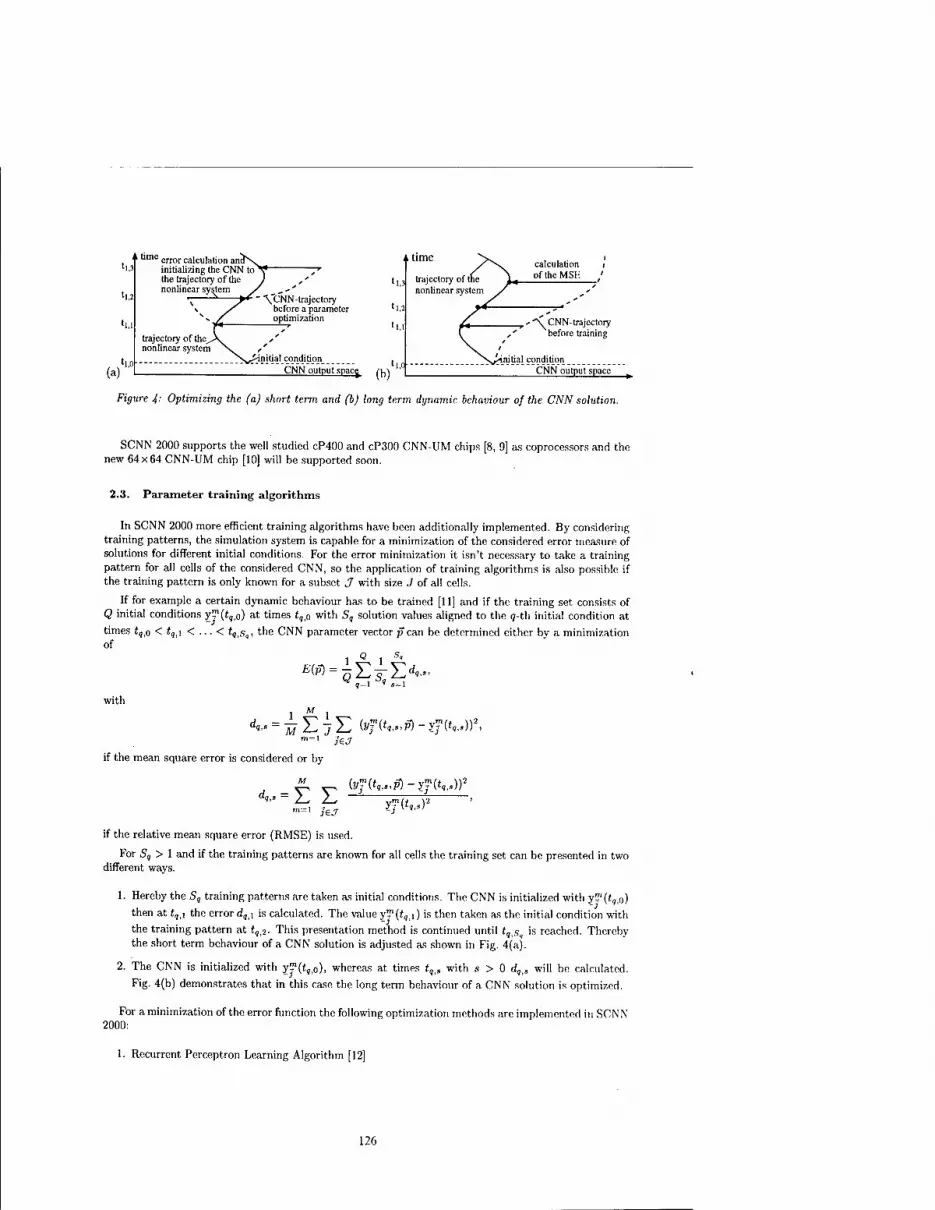
lu

'l error calculation am initializing the CNN to the trajectory of the nonlinear system

(a) '1.0

,. time

trajectory of the. nonlinear system

" *\ CNN-trajectory before a parameter optimization

'1.3

'1.2

11.1

^initialcqndition , CNN output space (D\

trajectory of the nonlinear system

-initial condition CNN output space

Figure J,: Optimizing the (a) short term and (b) long term dynamic behaviour of the CNN solution.

SCNN 2000 supports the well studied cP400 and cP300 CNN-UM chips [8, 9] as coprocessors and the new 64x64 CNN-UM chip [10] will be supported soon.

2.3. Parameter training algorithms

In SCNN 2000 more efficient training algorithms have been additionally implemented. By considering training patterns, the simulation system is capable for a minimization of the considered error measure of solutions for different initial conditions. For the error minimization it isn't necessary to take a training pattern for all cells of the considered CNN, so the application of training algorithms is also possible if the training pattern is only known for a subset J with size ./ of all cells.

If for example a certain dynamic behaviour has to be trained [11] and if the training set consists of Q initial conditions y™(i,,o) at times t,i0 with S, solution values aligned to the q-th initial condition at

times t?io < i,,i < ... < i,,s,, the CNN parameter vector p can be determined either by a minimization of

1 Q 1 5<

Ed«.» with

1 M 1

jSJ

if the mean square error is considered or by

di-> = E E — J6J

yf(tq,,y2

if the relative mean square error (RMSE) is used.

For Sq > 1 and if the training patterns are known for all cells the training set can be presented in two different ways.

1. Hereby the S, training patterns are taken as initial conditions. The CNN is initialized with y™(tq,o)

then at tqii the error d,,i is calculated. The value y™(r,,i) is then taken as the initial condition with

the training pattern at t,]2. This presentation method is continued until t,.s, is reached. Thereby the short term behaviour of a CNN solution is adjusted as shown in Fig. 4(a).

2. The CNN is initialized with y?(*,,o), whereas at times t,|S with s > 0 d,,, will be calculated.

Fig. 4(b) demonstrates that in this case the long term behaviour of a CNN solution is optimized.

For a minimization of the error function the following optimization methods are implemented in SCNN 2000:

1. Recurrent Perceptron Learning Algorithm [12]

126

2. Simplex method [13]

3. Powell's method [13]

4. Simulated Annealing [13]

5. Evolutionary Algorithm [14]

6. Recurrent Back Propagation Algorithm [15]

7. Conjugate Gradient Method [13]

8. BFGS-algorithm [13]

Methods 1 - 5 do not need any gradient information, whereas all other optimization methods are gradient based algorithms. The gradient is either approximated by

dE(p) _ E(plt... ,pq + (h ■ pq),... ,pQ) - E(j>u ... ,pq,... ,pQ)

dpq (h-Pq)

or 9E(p) = E(pi,. ..,pg + (h- pq), ...,pQ)- £(pi,.. ■ ,p, - (ft • pq), ...,PQ)

dp„ 2(ft • p„)

with h representing the stepwidth of the gradient calculation, which allows also an application of the gradient-based training algorithms to CNN-hardware.

With SCNN 2000 following CNN parameters and fuctions can be determined during a training pro- cedure

• the weight functions a(-), &(■), b(') and &(•) either translation variant or translation invariant defined by polynomial functions and tabulated functions,

• a translation variant or invariant bias and

• the output functions /(•) and g(-) defined by tabulated functions.

In order to minimize the number of parameters to be determined by a training algorithm it is possible to

• mark different template elements so they will not be changed during a training procedure,

• set different template elements of one template equal to other elements, so only one representative has to be determined during a parameter training, which is very efficient for template symmetries and

• train only a subset of all parameters of a tabulated function e.g. by assuming a symmetric function.

In the case that a time consuming parameter training has to be submitted to a queuing system with a limited calculation time, we have implemented the feature to stop the parameter training after a user defined time and save all the settings of the current parameter training on the hard disk. SCNN 2000 can be terminated and the parameter training can later be continued by a new SCNN 2000 process.

2.4. IO-Operations

2.4.1 Images

Different image formats are implemented for IO-operations concerning cell states, cell inputs, cell outputs, training patterns as well as for translation variant bias, resistors and capacities. Additionally to the SCNN own Rfnet- (ASCII) and Pfm-format (binary floating point format), SCNN 2000 can also handle the PNM-format, CNI-format and the RAW-binary format. Furthermore, the SCNN 2000 distribution includes different tools for a conversion of these and other image formats.

127

2.4-2 Templates and Output functions

The templates and user-defined output functions are stored in ASCII.

2.4.3 Project files

Often used settings of SCNN can be saved in the SCNN PRJ-format, which is a platform independent binary format. SCNN 2000 can handle all PRJ-formats of older SCNN versions.

3. Conclusion

SCNN 2000 is a precise, flexible and efficient tool for simulating CNN. It allows nearly arbitrary network structures and eel! couplings. Especially, higher order problems can be treated with SCNN 2000. Since it works under different operating systems it can be used as a common simulation environment even in heterogeneous computer networks. The implemented training algorithms are very efficient tools for designing certain CNN. Furthermore CNN-UM chips can easily be used as mathematical coprocessors. SCNN 2000 is a common simulation-chip environment for different CNN.

4. References

[1] Kunz, R., Tetzlaff, R., and Wolf, D.: "SCNN: A Universal Simulator for Cellular Neural Networks", Proc. CNNA, pp. 255-259, Seville, 1996.

[2] Kunz, R., Loncar, A. and Tetzlaff, R.: "SCNN 2000 - Part II: The Simulation Control System", submitted for publication at the CNNA, Catania, 2000.

[3] Chua, L.O. and Yang, L.: "Cellular Neural Networks: Theory and Applications", IEEE Trans, on Circuits and Systems, Vol. 35. Nr.10, pp. 1257-1290, 1988.

[4] Greville, T.N.E.: "Theory and Applications of Spline Functions", Academic Press, New York, 1969.

[5] Tetzlaff, R., Kunz, R., Ames, C. and Wolf, D.: "Analysis of Brain Electrical Activity in Epilepsy with Cellular Neural Networks (CNN)", Proc. ECCTD, pp. 1007-1010, Stresa, 1999.

[6] Tetzlaff, R., Kunz, R. and Geis, G.: "Analysis of Cellular Neural Networks with Parameter Devia- tions", Proc. ECCTD, pp. 650-654, Budapest, 1997.

[7] Tetzlaff, R., Kunz, R. Geis, G. and Wolf, D.: "Minimizing the Effects of Tolerance Faults on Hard- ware Realizations of Cellular Neural Networks", Proc. CNNA, pp. 385-390, London, 1998.

[8] Espejo, S., Rodriguez-Vazquez, R. and Dominguez-Castro, R.: "A 1 /iro CMOS Cellular Neural Network Universal Machine", Proc. ECCTD, Vol.2, pp. 893-896, Istanbul, 1995.

[9] Cruz, J.M., Chua, L.O. and Roska, T.: "A Fast, Complex and Efficient Test Implementation of the CNN Universal Machine", Proc. CNNA, pp. 61-66, Rome, 1994.

[10] Espejo, S., Dominguez-Castro, R., Linan, G., and Rodriguez-Vazquez, A.: "A 64x64 CNN universal chip with analog and digital I/O", Proc. ICECS, Lisbon, pp. 203-206, 1998.

[11] Tetzlaff, R., Loncar, A. and Wolf, D.: "Modelling Chaotic Systems by Cellular Neural Networks", Proc. ICNF, pp. 207-10, Hong Kong, 1999.

[12] Gezelis, C. and Karamahmut, S.: "Recurrent perceptron learning algorithm for completely stable CNN", Proc. CNNA, pp. 177-180, Rome, 1994.

[13] Press, W.H., Flannery, B.P. and Teukolsky, S.A.: "Numerical Recipes in C: The Art of Scientific Computing", 2nd Edition, Cambridge University Press, New York, 1992.

[14] Kunz, R. and Tetzlaff, R.: "Evolutionary Learning Strategies for Cellular Neural Networks", sub- mitted for publication at the CNNA, Catania, 2000.

[15] Balsi, M.: "Recurrent Back-Propagation for CNN", Proc. ECCTD, pp.677-682, Davos, 1993.

128

2000 6™ IEEE International Workshop on Cellular Neural Networks and Their Applications Proceedings

SCNN 2000 - Part II: The Simulation Control System

R. Kunz, A. Loncar and R. Tetzlaff

Institut für Angewandte Physik, Universität Prankfurt Robert Mayer-Straße 2-4, 60054 Frankfurt a.M., Germany

phone: +49 69 798 28317, fax: +49 69 798 28865 R.Kunz@rz.uni-frankfurt.de

ABSTRACT: In this paper the control system of SCNN 2000 [2], a universal simu- lation system for Cellular Neural Networks is introduced. It performs all input-output operations. The presented control system is based on the universal scripting language SCNNS, the SCNN shell and a graphical user interface. All three subsystems are necessary for a full functionality of SCNN 2000. The different parts of the control system, followed by examples of 3-dimensional modelling applications of the control system will be discussed in detail.

1. Introduction

Since the first introduction of SCNN in 1996 [12] various extensions have been implemented, e.g. an extended external programmability, which allow functional extensions easily. Furthermore, a modern graphical user interface and a powerful shell environment has been added. Therefore an external scripting language SCNNS has been developed and firstly introduced in an early version of SCNN 4 [3], In SCNN 2000 beside all old features a new improved functionality and new SCNNS commands have been implemented. Fig.l shows the internal structure of SCNN 2000 and the SCNN control system. The

High-level interface

Low-level interface

Xll SCNN shell

SCNN script

Translation unit

SCNN interpreter

Kernel SCNN 2000 simulation and training methods

1 SCNN control system

Figure 1: Components of SCNN 2000 and their interactions.

elements of the SCNNS language are analyzed and interpreted by the SCNN interpreter, which is a component of the SCNN shell. With this shell simple commands or complete programs, so called scripts will be executed in an interactive mode. It is the basic command line interface for a user. Beside all built in functionality, it supports the execution of arbitrary commands provided by the underlying operation system, thus allowing a combination of built in SCNN commands with i.e. file creation, copying, compiling and other tasks.

To support user by performing simulations or training procedures an extended graphical user interface is implemented in SCNN 2000. Despite older versions, which allow some limited actions only, the com-

0-7803-6344-2/00/$10.00 ©2000 IEEE 129

pletely rewritten interface allows all possible operations of SCNN 2000. The simulation kernel finally is connected through the interpreter to all other interfaces. The three main control concepts, the scripting language, the shell and the graphical user interface will be introduced in the following sections.

2. The SCNNS language

Like many other modern programming languages SCNNS consists of basic programming tokens, which are keywords, variables and commands. Loops and the ability of basic calculations such as additions or multiplications are included. Each command controls a certain part of the SCNN 2000 simulation kernel. The scripting language is useful to generate larger concatenated simulations or complex learning procedures. It offers the full functionality of a CNN Universal Machine [8]. Generally a SCNNS command is defined by

command [keyword ]["name" [[specifier ][expression ];.

Except the initial command and keyword, all other parts are optional and can differ between different commands. A command here directs the type of command to be initiated, while the keyword specifies the desired operation. The optional quoted name describe an internal SCNN 2000 variable, while the optional specifier controls the assignment of values. Finally expression can be any arbitrary calculation by using the supported basic calculation routines. A line of SCNN script is always terminated with a ";", this is different to older versions, nevertheless commands of older versions are also accepted due to compatibility reasons. Some examples are given in the following tables. In the current release of SCNNS there are more than 20 different commands, the mostly used are shown and described in Table 1. As

command explanation SCNN header of every script indicating a SCNN script set modifies internal control variables load loads arbitrary data save saves arbitrary data exec executes external commands such as dir, copy etc. start starts the simulation kernel

Table 1: Some typical commands of a SCNN script, refer to the users manual for a full list.

mentioned above, all commands except the initial SCNN must be followed by a keyword, describing exactly a command. SCNN 2000 knows more than 30 keywords, which can be combined with different commands. Some of them are listed in Table 2. Furthermore as an example of the implemented optional

keyword explanation sim learn template var resistor

initiates a simulation initiates a training procedure the command concerns a template modifies an internal variable resistor values are modified

Table 2: Some useful keywords of SCNNS. These keywords define exactly a command, i.e. starts a simulation.

"start sim"

descriptors and names, the set command with the flag or var keyword is introduced in the following, controlling every internal variable and flag of SCNN 2000. There are more than 80 different cases, a small subset mostly used is listed in Table 3. The following script of SCNN 2000 is a learning procedure of the well known average template with two images each consisting of 6400 cells.

3. The graphical user interface

SCNN 2000 provides a graphical user interface, which uses in most cases the scripting language of SCNN and hence is independent of the simulation kernel. Every user-system interaction will be converted

130

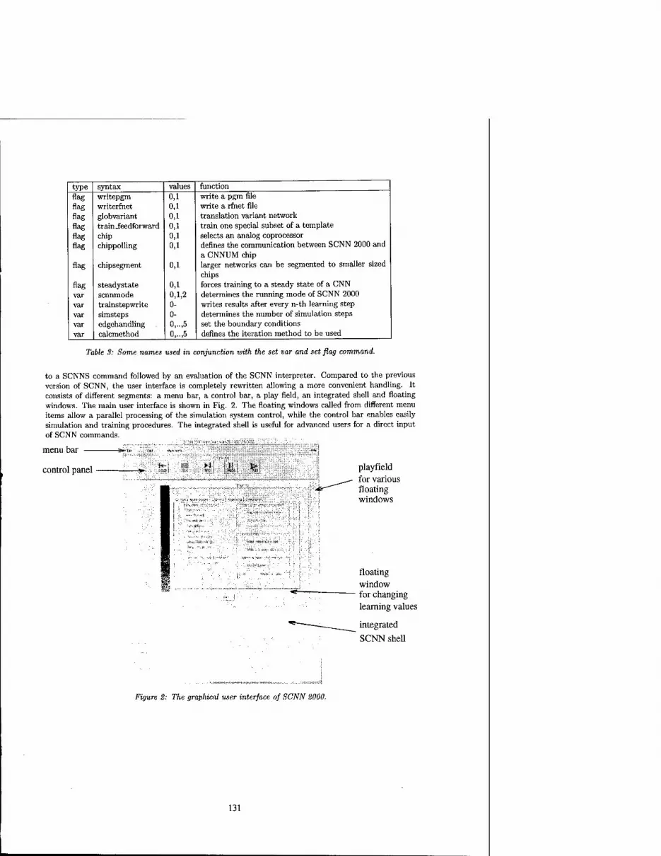
type syntax values function flag writepgra 0,1 write a pgm file flag writerfnet 0,1 write a rfhet file flag globvariant 0,1 translation variant network flag train-feedforward 0,1 train one special subset of a template flag chip 0,1 selects an analog coprocessor flag chippolling 0,1 defines the communication between SCNN 2000 and

a CNNUM chip flag chipsegment 0,1 larger networks can be segmented to smaller sized

chips flag steadystate 0,1 forces training to a steady state of a CNN var scnnmode 0,1,2 determines the running mode of SCNN 2000 var trainstepwrite 0- writes results after every n-th learning step var simsteps 0- determines the number of simulation steps var edgehandling 0,..,5 set the boundary conditions var calcmethod 0,..,5 defines the iteration method to be used

Table 3: Some names used in conjunction with the set var and set flag command.

to a SCNNS command followed by an evaluation of the SCNN interpreter. Compared to the previous version of SCNN, the user interface is completely rewritten allowing a more convenient handling. It consists of different segments: a menu bar, a control bar, a play field, an integrated shell and floating windows. The main user interface is shown in Fig. 2. The floating windows called from different menu items allow a parallel processing of the simulation system control, while the control bar enables easily simulation and training procedures. The integrated shell is useful for advanced users for a direct input of SCNN commands.

menu bar

control panel ■ :■*•-: £§ >1 111 I >\ playfield for various floating windows

floating window for changing learning values

integrated

SCNN shell

Figure 2: The graphical user interface of SCNN 2000.

131

Code Comment SCNN keyword defining the type of script. set var "scnnmode"=2; sets the operation mode of SCNN to a batch job operation. set flag " train Jeedback"=l; enables a training of the feedback template and set flag "train_bias"=l; of the bias value load template 0 n state loads the initial template and "average.ini tem" load img rfnet 0 bias "average.bias" the initial bias. set var "simsteps"=50; defines the number of simulation steps set var "population"=500; for the evolutionary algorithm define the population size and set var "parents" =50; the number of parents, set var "start_variation" = 10; the variation of the individuals and set var "initialmode"=0; their distribution. set var "crossover" =0.05; defines the cross-over rate. set flag "steadystate"=l; train for a steady state set var "trainsteps"=5000; no. of iteration steps during a single batch session set var "trainmethod"=2; selects the evolutionary algorithm addtotrainlist pgm 0 ref adds a reference image to a list of files used during optimization "picturel.pgm" addtotrainlist simnow pgm 0 state adds another file and performs a simulation immediately "picture2.pgm" addtotrainlist pgm 0 ref adding some more files to the list "picture3.pgm" addtotrainlist simnow pgm 0 state "picture4.compact.pgm" start learn now the learning starts save template 0 state when done, save the new found " average.ini tem" save img rfnet 0 bias "average.bias" values exec "/usr/local/bin/llsubmit executes a shell command for resubmitting a batch job 00d0.cmd" # restart same job this is a comment end end of script

Table 4: Script to determine the average template with SCNN Script.

4. Simulation examples

As a simple example the simulation of a 3 dimensional diffusion network with two fixed cell states and a Dirichlet boundary condition was performed. The considered network with 80x30x20 cells is shown in Fig.3. In our example all cells except the two cells with fixed state values are initialized with Zj(0) = 0. A precise simulation with SCNN 2000 has been observed. The script given in Table 5 leads to the desired actions of SCNN 2000. Some slices of the 3-dimensional solution are depicted in Fig. 4.

5. Conclusion

As we have shown, new programming abilities and a platform independent realization allows a broad range of applications with the new simulation system SCNN 2000. Results can be obtained with the universal computing language SCNNS. The SCNN interpreter processes working requests from its sub- systems, like the SCNN shell or the scripting language and sends the desired tasks to the simulation kernel allowing flexible extensions for future realizations.

132

4 I 3 ici

T

30 cell:

Fixed black cell (x = 1)

Fixed white pell ■*■ <T=H)

Boundary cells gray (x=0)

*S 20 cells

' All other cells: gray(x=0)

80 cells

Figure 3: Initial condition for the S-dimensional diffusion equation.

Code Comment SCNN; identifier set var "scnnmode"=2; set the batch job mode load template 0 n macro load the appropriate template "diffusion3d.macro;" load img rfnet 0 state "picture3d.rfnet;" and the initial image set var "simsteps"=50; do 50 simulation steps start sim; start the simulation save img rfriet 0 bias "result3d.rrnet"; save the result end; quit

Table 5: Script for a simulation of a S-dimensional diffusion network.

Figure 4: Two slices in z-direction of the resulting CNN output for the diffusion equation.

133

6. References

[1] R.Kunz and R. Tetzlaff: " Introducing Evolutionary Strategies for Learning with Cellular Neural Networks", to be publicated at the CNNA, Catania, 2000.

[2] A. Loncar, R. Kunz and R. Tetzlaff: " SCNN 2000 - Part I: Basic Structure and Features of the Simulation System for Cellular Neural Networks", to be publicated at the CNNA, Catania, 2000.

[3] R.Kunz: " SCNN User Documentation", http://ww.rz.uni-frankfurt.de/fbl3/e_ag-rt/SCNN/

[4] V.Cimagalli and M.Balsi: " Cellular Neural Networks: A Review"; Proc. 6th Italian Workshop on Parallel Architectures and Neural Networks, Vietri sul Mare, Italy (1993)

[5] J.A. Nossek: " Design and Learning with Cellular Neural Networks"; Proc. IEEE CNNA 94, Rome, pp. 137-146 (1994)

[6] R. Tetzlaff, R. Kunz and G. Geis: " Analysis of Cellular Neural Networks with Parameter Devia- tions"; Proc. IEEE ECCTD 97, Hungary, Vol 2., pp.650-654 (1997)

[7] L.O. Chuaand L. Yang: " Cellular Neural Networks: Theory and Applications"; IEEE Transactions on Circuits and Systems vol. 35, pp. 1257-1290 (1988)

[8] T. Roska and L.O. Chua: " The CNN Universal Machine: An Analogic Array Computer"; IEEE Transactions on Circuits and Systems II, vol.40 pp. 163-173, March 1993.

[9] Espejo, S. Rodriguez-Vazquez, R. Dominguez-Castro, R.: "Al /.m CMOS Cellular Neural Network Universal Machine"; Proc. ECCTD'95, Vol. 2, S. 893-896, Istanbul, (1995).

[10] J.M.Cruz, L.O.Chua and T. Roska: " A Fast, Complex and Efficient Test Implementation of the CNN Universal Machine"; Proc. IEEE CNNA 94, Rome, pp. 61-66 (1994)

[11] T.Roska et. al.: " CCPS: CNN Chip Prototyping System"; Version 2.1, Budapest, 1996

[12] R. Kunz, R. Tetzlaff and D. Wolf: " SCNN: A Universal Simulator for Cellular Neural Networks"; Proc. IEEE CNNA 96, Sevilla, pp. 255-260 (1996)

[13] T.Roska et. al.: " CCPS: CNN Operating System (COS)"; Version 2.1, Budapest, 1996

[14] T.Roska and L.Kek: " CSL: CNN Software Library"; Version 7, Budapest, (1997)

134

2000 6™ IEEE International Workshop on Cellular Neural Networks and Their Applications Proceedings

Regularization-Based Continuous-Time Motion Detection by Single-Layer Cellular Neural Networks

Marco Balsi

Inter-University Center for Research on Cognitive Processing in Natural and Artificial Systems and

Department of Electronic Engineering, "La Sapienza" University of Rome via Eudossiana 18 Rome, Italy 1-00184. Tel. (+39) 06 4458 5485 Fax (+39) 06 4742647

balsi@tce.ing.uniromal .it - http://tce.ing.uniromal .it/balsi.html

ABSTRACT: Regularization theory is proposed for systematic design of linear- and nonlinear- connection-based Cellular Neural Networks (CNN). In this paper, after stating the basics of regularization-based design ofCNNs, such methodology is applied to the problem of continuous-time motion field estimation in moving images. A single-layer solution is thus obtained and simulated, paving the way to full two-dimensional focal-plane real-time motion detection circuit implementation.

1. Introduction

The "inverse" problem of solving equation Mz = d (1)

for z given M and d, where in the general case z and d are arrays, and M is a nonlinear operator, is well-posed (according to Hadamard's definition) when it admits a unique solution, that depends continuously on the data.

Real-world inverse problems of engineering, physics, mathematics, etc. are very often ill-posed [1], e.g. because the data are noisy, so that an exact solution does not exist, or because the data only exist on a subset of the domain, so that the solution is not unique. Converting an ill-posed problem into a well-posed one is known as regularization [2],[3] and is accomplished by associating to problem (1), the problem of minimizing the functional

|Mz-rf|2+A||Pz|2. (2)

Operator P is a constraint operator (also called regularization operator, or stabilizer) that forces the solution to belong to a suitable subspace, i.e. have the characteristics that are expected for the solution (e.g. smoothness), and X controls the trade-off between enforcing the constraints and fitting the data exactly.

The variational principle induced by functional (2) can be equated to (pseudo-) energetic functions of analog electronic circuits and neural networks [4-8]. In this way, hardware architectures were proposed for real-time computations associated to ill-posed problems. Actual employment of such solutions in practical problems has been limited by the fact that special-purpose analog circuitry should be integrated in systems largely based on programmable digital hardware.

Cellular Neural Networks (CNN) [9] are massively parallel analog nonlinear processing arrays which can be efficiently realized in analog integrated electronics [10]. They find application in problems defined in space, which can be solved by local computation and information diffusion. Typical problems in this class are those of (nonlinear) image processing and feature extraction.

Design of CNN solutions for specific problems is hardly a systematic procedure. Most often, the designer has to rely on intuition and heuristics and has no control on optimality of the solution. Regularization theory provides a systematic method for designing CNNs. In this way, analog processing on such massively parallel hardware platform can become a realistic option for solving ill-posed practical problems.

In this paper, we consider in particular the problem of motion detection in images. Such problem is of great practical importance in communications, vehicle guidance, etc. Since computation of the apparent velocity field is very computation-intensive, research on architectures capable of real-time processing is very active. In the field of CNNs the most important results have been obtained by using the approach based on tuned spatio- temporal filters [11],[12]. This approach, however has some drawbacks: velocity is only estimated on a discrete set of possible values, and processing for each value must be performed separately (so that continuous time operation is practically unfeasible). The author considered [13] an alternative continuous-time solution based on a regularization approach, but the architecture obtained in the cited work involved a double-layer structure.

The paper is organized as follows: Section 2 contains a brief review of regularization theory and its application to the design of electronic circuits; Based on this theory, in section 3 a design procedure for CNNs solving regularization problems is established. Section 4 deals with problems involving nonlinear operators, and in particular motion field calculation. In Section 5 a simulation example is given, and Section 6 concludes the paper by indicating directions of further research.

0-7803-6344-2/00/$10.00 ©2000 IEEE 135

2. Analog electronics and CNNs for regularization

In the following, we shall consider discrete one- or two-dimensional space as domain of definition of our variables, without loss of generality. Let us consider first the case when operators M and P are linear, so that they are defined by matrices. We shall use the following notation:

(Mz),. =5>0Z/; j

We shall denote arrays will bold letters (e.g. M), and their elements as scalars (same letter in italics) with indices. One element of an array expression is indicated by using brackets with a subscript, as above.

When My is invariant to translation, we shall use the kernel matrix ((A/,..)) in one dimension, or

\\M/C_j;i_j)) in two dimensions, and call it again M. when no ambiguity ensues.

Writing functional (2) in terms of inner products we obtain that (M z - d, M z - A) + A(P z, P z)

is equivalent (neglecting a constant (d, d^ term) to:

z, M'MZ\ + X(Z, P'P Z\-2(Z, M* dV (3)

where O is the adjoint operator to O Eq. (3) may be identified with the energy, or pseudo-energetic function of a suitable electric circuit, so that

such circuit obeys the same variational principle as the problem we want to solve [4,6]. Cellular Neural Networks are described by the following equations [9]:

dx-

dt jeNr{i) jeNr(i)

where x, is the state of cell/'; «,• represents external input to cell;', t, is a threshold; Nr(i) is the set of indices of cells belonging to a neighborhood of cell i of radius r (which we shall just denote as N unless ambiguity ensues); A and B are weights (transconductances when v and u are voltages), which are space-invariant (cloning templates: In one dimension Ay = Aj-i, in two Ay^ = Aji_i.._/);.

In this case, following [6], it is useful to consider an energy function written as follows

/ I je N i ye A' /

When A is symmetric, this is a Lyapunov function that is minimized by operation of the network, which settles in a minimum of it. In fact, if we start the network in the linear range of/and g, and an equilibrium exists in the same range, then it must be unique, and the network will settle in that minimum. This happens when Ajj < 1. Other classes of A matrices also guarantee asymptotically stable behavior (e.g. [14]).

If we write (4) as follows:

2£ = E *■ l(-4-K-2I *■ XKK■+5X- a.-). (5) i jsN i jeN i

where A = A — I, and define

(a,b) = X«,A,

we can identify in eqs. (3) and (5) y with z, u with d,

and

((M*M+AP>»= 1{-Äy)yj. (7) j<=N

In this way, the two equations are equal if t = 0 . We shall consider this last condition valid in the following, but we point out that an additional term of the form (z, t) may be necessary to accommodate for non- homogeneous boundary conditions [15] in (3), and this can be readily identified with the last term in (5)

136

3. Designing CNNs for regularization

On the basis of the theory developed in the previous section, we are now in a position of identifying the class of problems that can be solved on the CNN architecture. In order to make the discussion gradual and practical, we shall consider relevant cases as a reference.

A widely used class of regularization functions in one dimension is that of Tichonov's stabilizers: \2

'"'HM^h When Cr is independent of <!;, the pertinent operator can be discretized in space in the form

*LpH*J

For instance, in approximation of functions defined on a continuous space from a finite number of samples, problem (2) can be stated as finding the function that optimizes jointly (according to the X chosen) the criterion of fitting the data (M is identity) and that of smoothness. In this case, the regularizing function is usually taken as

\\Pzf = f [z"(i*)]2 dE, , where P can be discretized as £ pj-iz] with P = & ~ 2 J ■ jeNi( i)

We shall develop this example in detail to show, in a simple case, how the appropriate CNN templates are designed.

As M = M" = [l], from (6) we immediately obtain B = [l]. In order to compute A, we need to obtain the

kernel matrix of P P, which we shall denote as R. It is easy to see by expanding the definition of adjoint

operator, that P, = P_t, (by the way, P* = ¥T in two dimensions). Therefore, one obtains

Ri=lPiPi+j, j

where we intend that Pj = 0, whenever / is out of the range of indices of P (self-correlation of. matrix P).

Therefore, we obtain R = [l -4 6 -4 l], and from (7)

A = [-X 4X -2-6X 4X -X}. The procedure outlined is obviously extended to more than one dimension and to any linear local operator.

In two dimensions, several kinds of operators involving partial derivatives [1], in the form

y c -

can be treated with the same techniques. Stabilizers in this class (which we shall call two-dimensional Tichonov stabilizers) are used e.g. for surface interpolation and approximation, shape from shading, optical flow, smoothing (especially as pre-conditioning for edge detection). As an example, the functional used in [8] contains a heuristic regularization functional that can be considered as a discretized Tichonov stabilizer for p=l.

4. Nonlinear operators: Motion detection

When M or P are nonlinear, it is not possible to apply straightforwardly the techniques developed in the previous section. However, similar procedures can lead to solutions that can be implemented on a modified CNN architecture, or discretized in time and processed on the CNN-UM.

The case of nonlinear M(z) can be approached by a Newton-like method [1], or solution can be based on the particular form of regularization function used, e.g. when it has the form of entropy [5].

In the following, we shall consider the case of regularization-based motion detection. As we shall see, in this case the functions involved are in fact linear with respect to each variable, so that a procedure can be applied, that is very similar to the linear case.

' The task of recovering the apparent motion field from the evolution of light intensity in moving images, known as optical flow, was pointed out by several authors [17],[18],[1] as an ill-posed problem, and solved by regularization. This problem consists of estimating vector velocity; Therefore it is stated in two unknowns, written in the following as vector z. The approach of Horn & Schunck[17] is based on a nonlinear approximation operator and linear Tichonov stabilizer:

\\t. s2

1 d@£

137

f?d-z-(-dTf +IN2, (8) where we generically denote dy/dx as yx. This operator involves a multiplication of solution and data (the

fact that the data are diffentiated in time is not essential, because we might as well make reference to the time integral of d as the data).

The author considered implementation of Eq. (8) on a double-layer modified CNN architecture [13], obtained by confronting with CNN equations the Euler equation associated with it. Of course, the solution involves multiplication of inputs (data) with state (current solution), just as Eq. (8) does. This implies a departure from the standard CNN model with linear connections, but this possibility is considered for generalized nonlinear models [14]. As the need for a double-layer architecture is also an inconvenience, in the following we shall consider an alternative single-layer solution, and obtain it by the techniques developed above.

In order to have a single state variable in each cell, I propose to represent vector velocity components alternatively on the grid in a checkerboard pattern, so that in each cell the local state represents one Cartesian component of velocity, as its four diagonal neighbors, while the other four neighbors code the other component.

In order to fix ideas we shall consider a cell coding z" i.e. the horizontal component of velocity. The

II II2 stabilizing function for this component is Vz* . In this case, it is more convenient to consider a gradient

operator rotated 45° from the Cartesian axes, so that we can discretize it using nearest neighbors (remember that

the other nearest neighbors are samples of zy). The simplest discretization of such a directional derivative has kernel

0 o 1/V2 0 -1/V2 0 0 0 0

R =

Proceeding as in section 3, we obtain from P45P45 + P135P135 - R (where P135 is orthogonal to P45):

-1/2 0 -1/2"

0 10.

-1/2 0 -1/2

We then consider operator Mz = dxzx + dyzy = [dx,dy]-[zx, zy\ . It can be easily shown that (for

generic data s) M s = [dx, dy J i = [dxs, dys\ . Therefore,

M'MZ = [dX,dyf(dXZ:'+dyZy)= [(dXfzX +dydrZy,dydyZ* +(dyYz>] .

At a site coding z" we just need the first component of M M z, which we shall denote as \M'M z) . In

order to compute it, we must notice that zy is not available at the current site, but can be obtained as an average of neighbors by applying operator

[0 1/4 0

1/4 0 1/4

0 1/4 0

Therefore, \M M zf = [dx y zx +dxdYzy can be discretized ;

(M* MJ ■■ - dydy

— dydy 4 x f

(JxY

-dydy

-dydy

By using (6) and (7) we then obtain B* = [M j = [dx ], and

138

AI =

dydy 4 x r

■-dxdy -(dxf-2X --dxdY 4 4

-dydy

Cells coding z^ have the same template matrices with dx and dy exchanged.

Up to this point, we have considered d and its space and time derivatives as given. This permitted us to get straightforwardly to the formulation of the solution in terms of A and B. It is obvious that spatial derivatives can be obtained by simple local differences on the input array, that is, basically, by a sort of second level of B-type matrix.

5. Simulation example

In order to validate the results of previous section, a simulation of operation of the designed CNN is given in this section.

An artificial image was generated, that contains a textured circle moving horizontally against a still background filled with the same texture. The latter is generated by assigning Gaussian-distributed random values to pixel intensities.

Figure 1 shows the velocity field extracted, superimposed to the corresponding snapshot of the input image. The area of the object is outlined by the white circle. It is apparent that the result is consistent with Horn & Schunk's method performance: The essence of the motion field is captured correctly, but a relevant edge effect is visible due to the well-known "aperture problem" [18]. A tail effect is also present, again intrinsic to the method.

Figure 1: Optical flow extracted by the proposed CNN. True velocity is purely horizontal. White circle indicates object position

6. Conclusions and perspectives

A methodology has been proposed, to solve ill-posed problems in image processing by systematic design of Cellular Neural Neworks, based on regularization theory. The technique is straightforward for linear problems, and must be adapted to individual nonlinear problems.

It has be shown, that by applying such methodology to a relevant nonlinear regularization problem, namely motion field calculation, a single-layer CNN solution can be designed that works in continuous time.

The solution presented in this paper is in fact the most basic, and was obtained by employing Horn & Schunck approach. In fact, such approach was later developed by several authors, who searched for better smoothness constraint functions (e.g. [19]), especially in order to tackle its main drawback, i.e. wrong smoothing in the presence of occluding edges.

Development of this work will follow such studies. In particular, Nagel & Enkelmann's [20] approach appears to be particularly suitable to the CNN environment. In fact, such approach is based on estimating the position of

139

occluding edges, and preventing smoothing across them. This is basically analogous to the concept of "anisotropic diffusion" [21], that has already been employed in CNNs [22].

Simulations on real-life images is being performed. Of course, proper simulation of the system is only possible on artificial images, because no continuous-time image signal can be obtained using video cameras. Implementation of such CNN-based motion detection system must in any case involve integration of images sensors on board, which will also guarantee real-time operation.

References

[I] Bertero, M., Poggio, T.A., Torre, V., "Ill-posed Problems in Early Vision", Proc. of IEEE, vol. 76, pp. 869- 889,1988

[2] Tichonov, A.N., "Solution of Incorrectly Formulated Problems and the Regularization Method", Soviet Math. Dokl, vol. 4, pp. 1035-1038, 1963

[3] Morozov, V.A., "Methods for Solving Incorrectly Posed Problems", Springer, New York, 1984 [4] Poggio, T., Koch, C, "Ill-posed Problems in Early Vision: From Computational Theory to Analogue

Networks", Proc. R. Soc. London B, vol. 226, pp. 303-323, 1985 [5] Marrian, C.R.K., Peckerar, M.C., "Electronic 'Neural' Net Algorithm for Maximum Entropy Solutions of

Ill-Posed Problems", IEEE Trans. Circ. Syst., vol. 36, pp. 288-294, 1989 [6] Pati, Y.C., Krishnaprasad, P.S., Peckerar, M.C., "An Analog Neural Network Solution to the Inverse

Problem of 'Early Taction'", IEEE Trans. Robotics Autom., vol. 8, pp. 196-212, 1992 [7] Girosi, F., Jones, M., Poggio, T., "Regularization Theory and Neural Networks Architectures", Nenr.

Comp., vol. 7, pp. 219-269, 1995 [8] Güzelis,C, Günsel, B., "Cellular Neural Networks for Early Vision", Proc. of 1995 European Conf. on

Circuit Theory and Design (ECCTD '95), Istanbul, Turkey, Aug. 27-31, 1995, vol. 2, pp. 785-788 [9] Chua, L.O., Roska, T., "The CNN Paradigm", IEEE Trans. Circ. Syst.-l vol. 40, pp.147-156, 1993 [10] Domlnguez-Castro, R. et al, "A 0.8-u.m CMOS Two-Dimensional Programmable Mixed-Signal Focal-

Plane Array Processor with On-Chip Binary Imaging and Instructions Storage", IEEE J. Solid-State Circ, vol. 32, pp. 1013-1025, 1997

[II] Adelson, E.H., Bergen, J.R., "Spatiotemporal Energy Models for the Perception of Motion", J. Opt. Soc. Am. A, vol. 2, pp. 284-299, 1995.

[12] Shi, B.E., "A ID CMOS Focal Plane Array for Gabor-Type Image Filtering", IEEE Trans. Circ. Sysl.-I, vol.46, pp.323-327, 1999

[13] Balsi, M., Cimagalli, V., "Design of CNN Filters in Log-Polar Space", Proc. of 1998 International Symposium on Nonlinear Theory and its Applications (NOLTA'98), Crans-Montana. Switzerland, Sep. 14- 17, 1998, pp. 675-678

[14] Roska, T., Chua, L.O., "Cellular Neural Networks with Nonlinear and Delay-Type Template Elements and Non-Uniform Grids", int.j. circ. th. appl, vol. 20, pp. 469-481, 1992

[15] Marongiu, A., "Simulating Electromagnetic Field with Cellular Neural Networks", "Laurea" dissertation (in Italian), "La Sapienza" University of Rome, Italy, 1995

[16] Horn, B.K.P., "Parallel Networks for Machine Vision", Massachussels Institute of Technology, Al Lab. memo. no. 1071, 1988, also appearing in Winston, P.H., Shellard. S.A., "Artificial Intelligence al MIT: Expanding Frontiers", vol.2, pp. 437-471, MIT Press, Cambridge, 1990

[17] Horn, B.K.P., Schunck, B.G., "Determining Optical Flow", Artif Intell.. vol. 17, pp. 185-203, 1981 [18] Hildreth, E.C., "Computations Underlying the Measurement of Visual Motion", Artif Intel!., vol. 23, pp.

309-354, 1984 [19] Snyder, M.A., "On the Mathematical Foundations of Smoothness Constraints for the Determination of

Optical Flow and Surface Reconstruction", IEEE Trans. Pall. Ana! Machine Intel!, vol. 13, pp. 1105- 1114, 1991

[20] Nagel, H.H., Enkelmann, W., "An Investigation of the Smoothness Constraint for the Estimation of Displacement Vector Fields form Image Sequences", IEEE Trans. Pall. Ana! Machine Intel!, vol. 8, pp. 565-593,1986

[21] Perona, P., Malik, J., "Scale-Space and Edge Detection using Anisotropic Diffusion", IEEE Trans. Pall. Anal. Machine Intel!, vol. 12, pp. 629-639, 1990

[22] Rekeczky, Cs., Roska, T., Ushida, A., "CNN-Based Difference-Controlled Adaptive Non-Linear Image Filters", int.j. circ. th. appl., vol. 26, pp. 375-423, 1998.

140

2000 6™ IEEE International Workshop on Cellular Neural Networks and Their Applications Proceedings

Heteroassociative Memories via Globally Asymptotically Stable Discrete-time Cellular Neural Networks

Giuseppe Grassi Dipartimento di Ingegneria dell'Innovazione, Universita di Lecce, 73100 Lecce, Italy

(giuseppe.grassi@unile.it)

Giuseppe Acciani Dipartimento di Elettrotecnica ed Elettronica, Politecnico di Ban, 70125 Bari, Italy

(acciani@poliba.it)

ABSTRACT: In this paper heteroassociative memories are designed using globally asymptotically stable Discrete-time Cellular Neural Networks (DTCNN's). The approach, which assures the global asymptotic stability of the equilibrium point by exploiting circulant matrices in the design phase, generates networks where the input data are fed via external inputs rather than initial conditions. This feature makes perceive the possibility of implementing heteroassociative memories via DTCNN's running in real time.

1. Introduction

Associative memories are neural structures able to store and recall arbitrary patterns (autoassociative memories) or pattern pairs (heteroassociative memories). Concerning this topic, until now Cellular Neural Networks (CNN's) or Discrete-time Cellular Neural Networks (DTCNN's) have been mainly designed by assuring the asymptotic stability of the equilibrium points [l]-[4]. Namely, the input data are fed via initial conditions and the outputs reach their steady state values at an equilibrium point which depends on the initial conditions. This means that, starting from initial conditions which represent a corrupted or incompletely specified set of data, the network output is able to reconstruct exact and complete information. However, this approach presents a drawback from the VLSI implementation point of view, that is, initial conditions are required to be set to zero each time the network is run. Obviously, this is an undesirable feature for networks running in real time [5]. The aim of this paper is to design DTCNN's where each trajectory converges to a unique equilibrium point, which depends only on the input and not on the initial state. The objective is achieved by exploiting the global asymptotic stability of the equilibrium point of DTCNN's with circulant matrices. The approach leads to define a nonlinear mapping from the space of external inputs to the space of steady state outputs, which can be exploited to design DTCNN's for heteroassociative memories. Since the input data are fed via external inputs rather than initial conditions [6]-[7], the approach makes perceive the possibility of implementing DTCNN's running in real time.

2. Heteroassociative memories design

By numbering the cells from 0 to N-l (see Figs. 1 and 2), the network dynamics are described by the following set of nonlinear difference equations [8]:

x(k + l) = Ay(k) + Bu + I y(k) = f{x(Jcj) (1)

where x = [x0 *, ... x„.J, y = \ya yx ... yN_J, « = [«„ u, ... u„.J,

/ = [/„ /, ... IN-J,f = [f(x0) /(*,) ... /(*„_,)]7',/(*,) = 1/2^ +l|-|x. _1|),/i=o,l, ...,

N-1. The sparse matrices A and B contain the feedback and the control parameters, respectively.

0-7803-6344-2/00/$10.00 ©2000 IEEE 141

2.1 Stability results

Assumption: Regarding the feedback parameters, the following one-dimensional space-invariant cloning template is considered:

\a(-r) ... fl(-l) o(0) a(\) ... a(r)] (2)

where r is the neighborhood radius, a(0) is the self-feedback, a(l) and a(-\) denote the connections with the next cells in the clockwise and counterclockwise order, respectively, and so on. Moreover, it is assumed that cell 0 is connected to cell A'-l. As a consequence, the feedback matrix A becomes a circulant matrix [8]-[9].

Definition: DTCNN's described by (1) are said to be globally asymptotically stable (GAS) if, for every constant input « e 9? , they have a unique equilibrium point x e 9!N which is GAS.

Theorem: DTCNN's described by (1) are GAS if and only if:

|5'(2^/A')| = |5;J:.r,a(A)exp(-y2^;?/JV)|<l ?=0, 1, ..., AM (3)

where the template spectrum S(a) = "Z^^a^cxpi-jhcu) is the discrete Fourier transform of the sequence

(2). The proof of the theorem is reported in [8],

2.2 Synthesis procedure

The constraint described by (3) (called frequency domain stability criterion since it can be checked by computing the discrete Fourier transform of the template elements) can be exploited for designing heteroassociativc memories. Concerning the feedback and control parameters, the DTCNN architecture is reported in Figs. 1 and 2, respectively. By taking into account these features in the course of the design method, DTCNN's with a globally asymptotically stable equilibrium point can be generated The key idea of the method is to choose a template (2) that satisfies the frequency domain stability criterion (3). Therefore, since the circulant matrix A is known, the objective becomes to compute the remaining network parameters R and /by properly solving the equilibrium equations By considering the bipolar patterns y' and «' (;-l, ..., m), which represent the stored vectors and the input

vectors, respectively, and by choosing a template (2) so that (3) holds, the equilibrium equations can be written in compact form as:

BU + l' = X - Ay (4)

where U = [u' u2 ... «"je*""", /'=[/ / ... /]e<RA'™, X = \x' x2 ... xm\e%N:"" and

/!,, =[/!>>' Ay2 ... Aym\= [A1 A2 ... A"\e'}lNx'". By defining the vector of the unknown

parameters as tc; = [*,„ bß ... AJ;V_, /Je SR1^"*1', it follows that:

Rw] = x] - ATyj 7=0, 1, ..., A'-1 (5)

where R = [uT j]e9l",xfN+'\ J = [\ 1 ... l]re9!m, Xj =[x) xj ... x;\e<H]x":,

Avj =\Aj A2 ... /I™je9i'"". Note that only the control parameters different from zero have to be

computed. By using a suitable index matrix [6], the following solution is obtained:

K]{x) -AL) y=0. 1, ...A'-l (6)

142

ij^B-s-g Fig. 1 The interconnecting structure related to the

feedback parameters (#=16).

□-EHH-Q i x i x I x i

B-B-E-B IX!XIX I

H-Q-H-H IX I XIX I

E-B-B-B Fig. 2 The interconnecting structure related to the

control parameters (#=16).

m m Trrrr

m

5S^ HE

Fig. 3 Design example: (a): input images; (b): output images.

Fig. 4 Design example: (a): noisy input images; (b): desired output images.

Fig. 5 Convergence rate as a function of the number of the stored patterns for HD-l (gray bars) and HD 2 (black bars).

143

where ivj (derived from Wj) contains the unknown network parameters and R* is the pseudo-inverse of

Rj (which in turn is a suitable matrix derived from R).

Note that the developed method also enables autoassociativc memories to be designed. Namely, by taking y' = «' the network is able to recall the memories y' starting from noisy patterns that correspond to noisy network inputs.

3. Simulation results

3.1 Error correction capability

A globally asymptotically stable DTCNN is designed to behave as heteroassociative memory. Fig. 3 shows the four pairs of (6x6)-pixel images used for the design (black pixel=-l, white pixel=+l). The procedure is carried out by taking #=36, a = 3 and by considering Chua's neighborhood with r=\ for the control parameters. Moreover, by choosing the feedback template

[O.OOI 0.001 O.OOl]

it is easy to show that the stability criterion (3) is satisfied. Since the circulant matrix A e y{36*36 js known,

it is now possible to compute B e <${36x36 and / e M36 by applying (6). Fig. 4 shows on the left the noisy- input images, whereas the obtained outputs are shown on the right. Simulation results highlight that the performances of the designed DTCNN arc characterized by a satisfying error correction capability. Similar results have been obtained by considering different circulant matrices A as well as different pattern pairs.

3.2 Storage capacity

Regarding the storage capacity of DTCNN's designed by the present method, an approach similar to the one developed in [6] has been considered. By taking a DTCNN with 9 cells, for each value of m between 1 and 9, the convergence rate (defined as the ratio of the number of input patterns which converge to the stored patterns to the number of all the possible input patterns, at a given Hamming distance HD) has been evaluated. The results are summarized in Fig. 5. The conclusion of the analysis is that a satisfying storage capacity is obtained. As expected, the percentage of patterns converging from HD=2 (black bars) drops off faster than the percentage from HD=\ (gray bars).

4. Conclusion

In this paper heteroassociative memories have been designed using globally asymptotically stable DTCNN's. The objective has been achieved by exploiting circulant matrices in the design phase. By taking into account that the input data arc fed via external inputs rather than initial conditions, the advantages of the proposed approach are that: a) both heteroassociative and autoassociativc memories can be designed, b) network running in real time can be generated.

Acknowledgement

This research has been supported by MURST under grant PRTN 1998

5. References

[1] ■ M. Brucoli, L. Carnimeo and G. Grassi, "Discrete-time cellular neural networks for associative memories with learning and forgetting capabilities", IEEE Trans. Circ. Syst. /, CAS-42, 396-399 (1995).

[2] D. Liu and A. N. Michel, "Sparsely interconnected neural networks for associative memories with applications to cellular neural networks", IEEE Trans. Circ. Syst. II, CAS-41, 295-307 (1994).

[3] A. N. Michel, K. Wang, D. Liu and H. Ye, "Qualitative limitations incurred in implementations of

144

recurrent neural networks", IEEE Control Systems, 15, 52-65 (1995). [4] M. Brucoli, L. Carnimeo and G. Grassi, "A global approach to the design of discrete-time cellular

neural networks for associative memories", Int. J. ofCirc. Theory cmdAppl., 24, 489-510 (1996). [5] C. Guzelis and L. O. Chua, "Stability analysis of generalized cellular neural networks", Int. J. of

Ore. Theory andAppl, 21, 1-33 (1993). [6] G. Grassi, "A new approach to design Cellular Neural Networks for associative memories", IEEE

Trans. Ore. Syst. I, CAS-44, 835-838 (1997). [7] G. Grassi, "Lyapunov diagonally stable matrices to design Cellular Neural Networks for associative

memories", Proc. of the 5,h IEEE Int. Workshop on Cellular Neural Networks and their Appl. (CNNA '98), London, 410-415 (1998).

[8] R. Perfetti, "Frequency domain stability criteria for cellular neural networks", Int. J. of Ore. Theory andAppl, 25, 55-68(1997).

[9] M. P. Joy and V. Tavsanoglu, "Circulant matrices and the stability of a class of CNNs", Int. J. of Ore. Theory andAppl., 24, 7-13 (1996).

145

2000 6™ IEEE International Workshop on Cellular Neural Networks and Their Applications Proceedings

SC-CNNs for Sensors Data Fusion and Control

in Space Distributed Structures

C. Amenta, P. Arena, S. Baglio, L. Fortuna, D. Richiusa, M.G. Xibilia, L. Vullo

Dipartimento Elettrico, Elettronico e Sistemistico University of Catania

V.le A.Doria, 6 - 95125 Catania - Italy

ABSTRACT: Analog modular architectures, based on the computational paradigm of State-Controlled Cellular Neural Networks, are considered in this paper to suitably manipulate signals obtained from multiple sensors measurement systems necessary for controlling deformations in space distributed structures. The design methodology to choose the Cellular Neural Network template coefficients such to obtain the desired "global" behavior is proposed together with some theoretical results that guarantee asymptotic stability of the system. An experimental prototype of this State-Controlled Cellular Neural Network for multisensor data fusion and control applications is presented, moreover the problem of controlling the deformation of a multiple link system is tackled.

1. Introduction

In this paper an architecture, based on the paradigm of State-Controlled Cellular Neural Networks (SC-CNNs) [1], is proposed both for multisensor data fusion [2] and for controlling space distributed structures. This system, here named Analog Cellular Networks (ACNs), takes its inspiration from the State-Controlled Cellular Neural Networks (SC-CNN) paradigm [1,3,4], ACNs are in fact arrays of locally interconnected analog cells arranged in a regular grid, whose processing is controlled by the values of the cloning templates. The peculiarities of ACNs consist in the fact that each cell of ACNs contains the sensing and the actuation part inside its structure, moreover the state-output function of the ACN cell matches the input-output function of the actuator. In the following a linear characteristics for both the sensor and the actuator will be considered and some sufficient conditions for the asymptotic stability of the whole structure will be derived, together with a design methodology for the template coefficient selection. The inclusion of saturation nonlinearities for the actuators allows to consider ACNs in the framework of classical CNNs [3, 4]. In this paper ACNs are used as analog modular circuits for conditioning signals gathered from a distributed measuring system where each ACN cell receives the sensor signal as input and drives one actuator with its output voltage. Due to the intrinsic characteristics of ACNs each cell output to the actuator will depend on the estimates of the whole set of sensors, without being actually connected with all of them; in fact only local connectivity is considered in the ACN paradigm thus exploiting modularity of the multisensor data fusion system.

Moreover the ACN system is used for obtaining suitable control signals for smart structures [5, 6]. Generally speaking, the term "smart structure" refers to complex systems where both sensing and actuation are involved and often integrated in the mechanical structures itself. Active flexible surfaces can be considered a typical example of smart structures. Often complex sensing architectures are needed and several sensors are used for gathering data to the signal processing unit. High computational capability, a real time processing and a space distributed parallel structure are therefore required to gather and manage efficiently the huge amount of information carried out from the sensor network.

Besides modularity, the main advantage of ACNs over the actual multisensor arrays lies in the possibility to control each actuator on the basis of "global" information regardless of having only "local" connections among neighboring cells [6]. The ACN behavior depends on the template coefficients value that must be accurately chosen. In this paper a novel methodology that allows determining the template coefficient values in accordance with the desired control law is introduced together with some theoretical result to ensure the asymptotic stability of the system. An experimental prototype is also presented: it consists in a smart distributed structure that, on the basis of collective information about external actions, can keep a desired shape against external disturbances.

0-7803-6344-2/00/$10.00 ©2000 IEEE 147

2. ACNs for data fusion and control

The basic idea developed in this paper is that ACN architectures allow to implement "global" functions on data obtained from distributed measuring systems having only "local" connectivity. In particular, each cell output is a function of all the ACN cells inputs without a direct global cell interconnection. This feature is appealing for applications in multisensor data fusion [2] and for distributed control systems. The architecture proposed for multisensor fusion and integration is a "circular", one-dimensional ACN as shown in Fig. 1: each "cell" input u,

, represents the output for the sensor St; each cell is connected via the state template (C) and the control template (B) to the "neighboring" cells. Symmetric templates are considered due to the "circular" topology adopted: C-fcj c0 cj ; B=[b, b0 b,].

U,ji-B(yH,l„M-C(i,j>;

B(' j). C(ij) Templates matrices

Yi=f(X)=hx,+u, Output function

Figure 1: The A CN architecture for multisensor data fusion and distributed control

If all the actuators are considered as working in the linear region, the state equations for a ACN with N cells, written in lexicographical order, are:

i\ =—- + c\X[f +CQX\ + C\X2 +blUff +2>o"i + b\u2

Xo , *2 = - + cl*l + c0*2 +Cl*3 + *l"l +*0"2 +*1"3 R (1)

Xff =—^- + C|XAr_1 +C0XN +C,X, + b1UN_l +b0UN + Vl

y\ =hx\+ hi\

y2=hx2+ku2 (2)

)>N = ktN + *"JV

148

sd

A suitable choice of the template coefficients allows to determine the behavior of the whole system while h and k are real coefficients to be determined taking into account the control action. Modularity is enhanced by adopting space-invariant values for the cell parameters, the templates and the output variable coefficients. Analytic conditions on the template coefficients must be stated in order to ensure asymptotic stability of the system which is a necessary condition to suitably process the cell inputs.

Proposition 1. One-dimensional, circular ACNs with symmetric templates are asymptotically stable if:

c0-^+2|Cl|<0 (3)

where R represents the resistance of the generic cell

This proposition can be simply verified by observerving that, whatever is the number of the ACN cells, the left part of rel. (3) represents an upper bound for the ACN state matrix eigenvalues. For the ACN architecture reported in Fig.l with Ncells, if eq. (3) is satisfied, referring to eq. (1), the asymptotic behavior can be written in matrix form as follows:

0 =CX +BU (4)

where 0,X,U are real vectors of dimension equal to the number N of cells, while C,B, are square real

matrices NxN. From eq. (4) it directly derives:

X=-CT'BU (5)

Due to the circular and symmetric structure adopted, if an odd number N=2n+1 of cells is considered, the state x, of the generic i-th cell will assume the following form:

« Xi = p(0,«)«,- + £ p(j, „)(ui+J + uH) (i = 1,..., AO (6)

with the following "periodic" boundary conditions: uo = u/g un*i = u:. The coefficients p(d,n) with (d=0,...,n) represent the weight of the input «,-, to the cell Cj, on the i-th cell

state Xi located d cells far from Cj. Such parameters are decided at the design stage, in order to ensure a control law for the structure. The design problem consists, for a given number of cells, in determining the template coefficients Co, C/, bo and bj that give the desired vector P*=[p*(0,n),...,p*(n,n)]. The desired coefficient parameter vector P*=\p*(0,n),...,p*(n,n)] is imposed to be the same for all the cells; under these conditions the same quantity is available at each cell site regardless of the network spatial dimension. As an example, for a ACN with five cells (n=2) it holds:

p(02) = (cl + c0cl ~ c\ + Co ~ 2c0 + l)*t) + Y-Cj ~ 2ci2 ~ 2CQC{ fa

(c0 -l + 2ci)(-2c0 -c0q +CQ +l + q -c\)

p^2) = I1+c0cl ~ci + 2c0 + cj]bx+ (ci -c\ -c0ci \ (7)

(co-l + 2ci)(-2c0-c0c1+co+l + ci-ci2)

p(2,2) = fel-WWfr (co-l + 2ci)(r2c0-c0c1+c0 +1 + C] -ci )

Equations (7) are linear with respect to the (bo, b{) unknowns and the design problem can be solved as an optimization problem with [6]:

149

:{HTHYH

TP- (8)

. I.

where the coefficient matrix H, obtained from (7), depends on (c», c,). These latter coefficients must be chosen in such a way both to satisfy the stability condition (3) and to minimize the difference \P*-P\ between the desired value for the parameters vector and the one obtained by back substituting (b0, b:), drawn by solving eq. (8) into eq. (7). In the case of N=5 the quantity \P*-P\, together with the stability condition (3), is reported in Fig.2 against (c„, C;). It can be derived that the closer the C template coefficients are to the stability condition (3), the smaller is \P*-P\ [6]. Finally, the cell parameters R and C are chosen based on both dynamic and stability considerations, while the h and k constant parameters allow to customize the cell output value.

Figure 2: Optimal choice of the C template coefficients for the "design problem" and for the "stability condition " of A CNs.

2.1 Remarks

By using classical approaches employed in arrays of linear systems one could easily obtain a weighted sum of the inputs to one actuator but, if this information is required in all the points of the structure, the complexity of the circuit would drastically increase because the global direct connection is required. This does not happen in the system here presented, that uses only local connections and exploits modularity for ensuring the same behavior regardless of the number of sensors involved.

Finally a remarkable issue is that although the structure presented is globally linear, saturation nonlinearities representing real actuators characteristics can be included without affecting the overall performance. In fact they cannot in any case alter the performance of the structure since, starting from the linear region, characterized by asymptotic stability, the analog signal processing and control allows to remain into the linear region in spite of any disturbance which could lead to saturation effects.

3. A prototype of a distributed control structure based on ACNs

The introduced ACNs are here applied to the control of a multiple link structure. In particular the goal is to maintain a desired shape in spite of external disturbing actions and, namely, the control problem consists in maintaining the symmetry of the structure in spite of external disturbing actions insisting on the joints.

The experimental system is shown in Fig.3. In this figure it can be observed an overview of the whole system and an exploit of both the analog circuit and the electro-mechanical sections.

In particular this latter is intended to be maintained symmetric, namely all the joints must realize the same

150

angle in spite of external disturbing actions. As an example if one of the joints is forced to enlarge all the other joints must enlarge such to maintain the structure symmetric with respect to its axes.

kW

Figurei: Pictures of the distributed structure realized and of the Analog Cellular Ne sensor outputs and for determining control signals.

ork adopted for managin

The sensor data fusion is necessary in such case, since information on the whole set of sensor readings is required in order to correctly control the actuators so as to provide the desired pre-specified shape to the overall structure. In order to reach the desired goal each actuator should operate on the difference between the "local" signal, coming from its own sensor output, and the average value on the whole set of sensor outputs; in such a way saturation phenomena can be avoided. In this sense the "smart" distributed control system could, in some of the joints, work in the same direction of the external action.

The ACN design consists in choosing the template coefficients such that the x, variables of each cell are proportional to the average value of the cell inputs. The cell output >>, depends on the difference between this average value and the "local" sensor output. This difference will drive each actuator. Experimental measurements on this circuit have been performed. The desired weighting function was fixed to P*=[ 1 1 1 1 1 ] and the template coefficients were determined as c„=0.3, C/=0.3, 6o=0.0019, i(=0.243. The actual values obtained with the realized circuit were P'M=[0.94 1.06 0.96 1.06 0.94] with a maximum relative difference not larger then 6%. In Fig. 4 some experimental results are reported: the output voltage of the ACN state x, input u, and output

x/ yi = '/xr — Ui are shown. In the experiment shown in Fig.4 a disturbance is applied to the central joint of the

structure. It can be observed as the "smart" control acts so as to contrast the deformation with the "central" actuator while working in the same direction of the joint deformation in the outer region.

151

1 i —1— Cell input/Sensor output

-0-Cell state

•if " Cell output/Actuator input

NL J Y ! i k< 1 „ >4

A «.'-. *""! r"' 1 1

Jf • • • Figure 4: Experimental measures on the Analog Cellular Network prototype

4. Conclusions

An analog modular architecture, named Analog Cellular Networks, for realizing multisensor data fusion and distributed control systems has been presented. The proposed architecture is based on the SC-CNN paradigm. Suitable methodologies for both the analysis and the design have been investigated. Applications of this paradigm to the field of smart structures have been proposed. Experimental results have been reported, referring to an analog prototype of measuring and control system, which shows the suitability of the proposed strategy. The kind of sensory data that can be fused by using this approach is quite general: in fact the proposed strategy doesn't depend on the sensor nature. In the paper the control of a multiple link mechanical structure is considered The approach results very appealing since it opens the possibility to apply the paradigm of ACNs and CNNs also to the field of distributed sensor processing and smart structures, since it combines the most important features of these architectures: local connectivity and global information processing. The introduction of the concept of an analog space-distributed network directly integrated with sensors and actuators is very important in the field of the control of structures extended in space, like large antennas for space applications or membranes. In such cases the possibility to have an analog, distributed sensing and control structure represents a real breakthrough.

5. References

[1]

[2] [3] [4]

[5]

[6]

P. Arena, S. Baglio, L. Fortuna, G. Managanaro, "State Controlled CNN : A New Strategy for Generating High Complex Dynamics", IEICE Transaction on Fundamentals of Electronics, vol. E79-A, no. 10, Oct. 1996. D.L. Hall, "Mathematical techniques in multi-sensor data fusion", Artech House, 1992. Chua L. O., "CNN: A Paradigm for Complexity", World Scientific, 1998 G. Manganaro, P. Arena, L. Fortuna, "Cellular Neural Networks: Chaos, Complexity and VLSI processing", Springer-Verlag, 1999. S. Baglio, S. Graziani, G. Manganaro, N. Pitrone, "Locally interconnected cellular architectures for multisensor data fusion", IEEE IMTC'96, June 1996, Brussels, Belgium. P. Arena, S. Baglio, L. Fortuna, S. Graziani, "Analog Cellular Networks for Multisensor Fusion and Control", accepted for publication on IEEE Transaction on Circuits and Systems-I

152

2000 6™ IEEE International Workshop on Cellular Neural Networks and Their Applications Proceedings

AUTO WAVES IN NONINTEGER ORDER CNNS

P. Arena, L. Bertucco, R. Caponetto, L Fortuna, G. Nunnari, D, Porto*

Dipartimento Elettrico, Elettronico e Sistemistico Universitä degli Studi di Catania

V.le A. Doria, 6,95125 Catania - Italy E-mail: parena@dees.unict.it

*STMicroelectronics - Soft Computing Group Stradale Primosole50, 95100 Catania-Italy

ABSTRACT: In this paper it is shown that complex spatio-temporal phenomena, usually met in physical and biological systems, can be reproduced by means of Cellular Neural Networks of non integer order. The template parameters are reported in the paper, together with some simulation results which show the suitability of the approach.

1. Introduction Recently the scientific community has been greatly interested in the study of complex phenomena taking

place in space-distributed dynamical systems, such as autowaves, self organizing patterns and Turing patterns. In fact, such dynamics are quite common in several scientific and natural fields: from biology to physics and chemistry. Of course, the possibility to implement them in simulators and, subsequently in circuit paradigms allows to reproduce them in real time. Until now third order chaotic circuits and second order slow-fast circuits have been considered. In the first case autowaves were considered as particular solutions of chaotic dynamics, while the second implementation allowed to understand that also particular oscillatory dynamics, not necessarily chaotic ones, were sufficient conditions for the generation of these phenomena. The possibility to implement autowaves, spirals and self-organizing patterns by using non integer order CNNs is explored in this paper. In particular two-layer non integer order CNNs are employed; the conditions for the onset of the self organizing phenomena are reported. Moreover a simulator is briefly discussed and some numerical results are introduced. Since low order fractional dynamical systems were indeed found able to show chaotic dynamics, autowaves could be found to be interesting solutions of chaotic dynamics in low fractional order CNNs.

2. Multi-Layer CNNs with Non-Integer Order Cells

A standard multi-layer CNN [1-3] (MCNN) can be represented by the following equation:

dx It) I L

Ci -^—if-W'J + Sf lAPS(i,j;k,l)*ysM(t) + dt S=l 1/6 NJi.j)

+ £ Bps('J;k.l)*uSM+ '%CPS(i,j;k,l)*xs,u) + lSJi (1) tteAUUJ >.l£H,(i.i)

*,j,(0) = xPm CXr>0, R,p>0

where: Je, y and u are the state, the output and the input of the condered cell; Nr is the rxr is the cell neighborhood; C and R are the capacitance and resistance of the cell; L is the number of layers of the CNN; the subscripts p,ij refer to the cell (/, j) belonging to the p-th layer; Xpj/0) are state initial conditions; A, B, I are the CNN templates.

The introduction of non integer order derivatives leads to :

0-7803-6344-2/00/$10.00 ©2000 IEEE 153

dqx (t) I '- C,, —f~ = -z-x^W + X YArs<U;k,l)*ySJ„<t) +

"' Kx, S-l UeN,{:.jl

+ X BK(i,j;k,l)*uSM+ 'Zcl,sa,j;k,l)*xSM)+Is, (2) tl€H,(l.ll kjen,li,i)

where 9 is the order of the Multi-layer CNN. Equations (2) can be considered as extension of the mathematical expressions for a non integer single layer CNN given in [4]. In solving such a kind of equation, non integer order integration must be used [5]. This operator is defined as follows:

d-g(t)_ 1 ,,. .1,-,./.1J. (3)

dt'" T(q)>;

V(*) being the factorial function. In order to build the numerical algorithm, we need a discrete approximation of relation (3). Taking T as the sample time and supposing g to be constant during this time interval, after some calculation it results [6]:

D-g(l)=g(l)

D-'ga+i^-^-Y^J+t^^^h-jr-ik-j-iA (4) i(i + q)P<> 2

<k>l)

The non integer order CNN, reported in (2) belongs to the most general array dynamic equation:

X(q) = f(x,t) (5)

whose numerical solution, derived by using expression (4), is given by:

xik + D^-^-^f^J+DJ+Di^-jy-ik-j-ir]

(*>D

For q<l an initial condition must be added to (6).

3. The Non Integer Order CNN Simulator

The simulator built to study complex phenomena in non integer order CNNs was written in the ANSI C language to allow high portability. It is called MCNNSm99 (Multi-layer CNN Simulator 1999); it is an upgrade of the CNN simulator proposed in [7]. The flow chart of MCNNSm99 is shown in Fig. 1. The main features of MCNNSm99 are the following: • possibility to simulate a CNN represented by non integer order differential equation; • possibility to simulate any number of layers; • different integration methods can be selected to solve differential equations (Euler, Runge-Kutta); • complex sets of CNN-based operations can be executed, both of unary type (a single image processed as the

initial state matrix and/or input matrix) and binary type (two images processed at the same time); • global reconfigurability of the CNN parameters and dimension; • the portability of the code used in simulator implementation (ANSI C); The graphic formats allowed are text format, binary format and Bitmap format.

154

The routines for non integer MCNN are realized as extensions of the procedures described in [4] for a single layer CNN. The Total Configuration File allows to configure all parameters of the Multi layer CNN.

User Interface Options:

• Layers Number and CNN Order (P, q) • Templates Maker (NxN, Linear and Non Linear) • Integration Parameters (RK4/Eul, Number Iterations, Integration

Step, CNN Order: Default 1.0) • Cell Circuit Parameters (Rx, C) • Inputs / Initial States • Boundary Condition (Zero-Flux, Thorus, Constant)

y

Total Confij (Default o

;uration File r Custom)

V i r

Input

Images

Initial State

Images ► State Equation definition

(Both Integer or Non-Integer CNN) *

• • • • • • 1 r

State Equations Integration (RK4/EULER)

w

i r v i • • • '

Output

Images

Fig. 1 - Flow Chart of the MCNNSm99 Simulator

4. Simulation of the Complex Phenomena In [8] the authors introduced a CNN built-up of second-order cells and able to generate autowave propagation. In fact, in literature such kinds of complex phenomena were also described as particular dynamics shown by third or higher order autonomous chaotic systems arranged in spatial topologies. Indeed it could be not surprising to find oscillations in single state variable fractional order cells. However, all the simulations performed revealed that all the oscillatory dynamics met did not give rise to autowaves. This fact is clear since autowaves are solutions of Reaction-Diffusion systems of the type activator-inhibitor. Therefore two different dynamics are needed for a single cell to be able to generate oscillations for autowaves. The template values for the two-layer CNN are the same as those ones reported in [8]. The study will be performed by considering non integer order cells built-up of two state variables.. Therefore a two-layer CNN with non integer order cells will be studied.

155

Here are reported the templates used to simulate the complex phenomena. Referring to eq. (2) for a two-layer CNN it results:

Ai - \i

(0 1 0

1 1.3 1

0 1 0

; Af2 - A,, (° 0 0\

0 -1 0

0 V

0 0

;B = 0;/.=-/, =-0.3.

AH the simulations will be performed by using image dimensions "46x46"and 256 gray levels. The boundary condition were fixed to Zero-flux in all cases. In Fig.2 the initial conditions for the onset of an autowave front are reported. In particular, the gray levels for a section for each layer are shown in Fig. 3.

Fig. 2: Initial conditions for the onset of an autowave front for the first layer (a) and the second one (b)

Fig. 3: Values for the initial conditions in a particular section of Fig. la and Fig. lb, respectively

m •

~5~ .~o~- o

o

"O

o

Fig.4: Snapshots showing the propagation of an autowave front and a circular autowave: Order 0.8 - Layer 1

Figure 4 shows the snapshots obtained from the first layer of a CNN of order q=0.8 for each layer. The particular initial conditions imposed to the first layer lead to the formation of an autowave front and of a circular unique wave arising from the simulation of an "inhomogeneity" in the medium, (see Fig.3a). Since the autowave front

156

and the circular wave have the same speed and the same propagation direction, no collision is seen during the propagation. In Fig.5 the initial conditions for the onset of a spiral wave are depicted for the first and the second layer, respectively.

Fig.5: initial conditions for the spiral wave onset

1 3"||~eT|[~eFj| Q)\\ @)|[©^[©] Order 0.5 - Layer 1 ^nrorsraß» Order 0.3 - Layer 1

^n^rareJiFsra T Order 0.1 -Layer 1

Fig.6: Propagation of a spiral wave for different values of the non integer order CNN

In Fig.6 it is possible to appreciate that the spiral wave succeeds in propagating even if the order of the cells of the two layers are very low. In particular, when the cell order decreases to 0.1, the spiral is somewhat out of shape, but its propagation takes place. One of the classical properties of spiral waves, the annihilation after collision, is appreciable in Fig. 8. In Fig. 7 the initial conditions are reported.

5. Remarks and Conclusions The simulations reported in the previous section show that complex self-organizing phenomena, such as autowaves and spirals can be obtained in non integer order CNNs. In particular, Fig.6 and Fig.8 reveal that the phenomenon is able to take place even when the order of each cell is very low. Moreover, in this case, the wave propagation takes place showing some kind of turbolence. Indeed, non integer order CNNs have been shown to be able to show chaotic dynamics also when a two state variable autonomous CNN is considered [9]. Therefore it cannot be excluded that also in the case of auto wave generation spatio-temporal chaos could be met. This topic is a subject of current research. Another important feature is that, although at a very early stage, some realizations of non integer order circuitssystems were proposed [10]. Under this perspective, the study of these phenomena becomes more attractive since a circuit realization could allow a real time implementation, avoiding the need of simulating very large dimensional systems. Taking also into consideration the key role that auto waves are assuming in important applications such as generation and control of artificial locomotion, a circuit implementation of such phenomena could lead to more sophisticated solutions to the above problem.

157

Fig.7: Initial conditions for the generation of two autowave fronts

C£ Q9 0 ■■■" <

^yiSJ Order O.S - Layer 1

Order 0.1 - Layer 1

Fig.8: Collision of two spirals; simulations performed for various non integer order cells

REFERENCES

[1] Chua L. O. and Yang L., Cellular Neural Networks: Theory. IEEE Transactions on Circuits and Systems Vol. 35 No. 10, October 1988, pp. 1257-1272.

[2] Chua L. O. and Yang L., Cellular Neural Networks: Applications. IEEE Transactions on Circuits and Systems Vol. 35 No. 10, October 1988, pp. 1273-1290.

[3] Chua L. O. and Roska T„ The CNN Paradigm" IEEE Transactions on Circuits and Systems Vol. 40 No. 3, March 1993, pp. 147-156.

[4] Arena P., Bertucco L., Fortuna L., Nunnari G., Occhipinti L., Porto D. CNN with Non-Integer Order Cells, CNNA 98, IEEE International Workshop on Cellular Neural Networks and Their Applications Proceedings, pp. 372-378, 14-17 London, April 1998.

[5] Ross B., Editor Fractional Calculus and its Applications, Berlin: Springer-Verlag, 1975. [6] Oldham K. B., Spanier J. Fractional Calculus, Academic Press, New York, 1974. [7]Bertucco L., Nunnari G., A Multi-Layer Cellular Neural Network Simulator for Image Processing

Applications, Proceedings of the third International ICSC Symposia on Intelligent Industrial Automation IIA'99 and Soft Computing SOCO'99, pp. 147-151, June 1999, Genova, Italy.

[8] P. Arena, S. Baglio, L. Fortuna, G. Manganaro, Self-Organization in a Two-Layer CNN, IEEE Trans. On Circuits and Systems, I: Fundam. Theory and Applic, Vol. 45 N°2, pp. 157-162, Feb. 1998.

[9] P. Arena, R. Caponetto, L. Fortuna, D. Poüo,"Bifurcation and chaos in non integer order cellular neural networks" Int. J. On Chaos and Bifurcation, Vol. 8, N°.7, pp.1527-1539, 1998.

[10] P. Arena, L. Fortuna, D. Porto, "Chaotic behavior in noninteger-order cellular neural networks" Physical Review E, Vol. 61,1, pp.776-781, Jan. 2000.

158

2000 6™ IEEE International Workshop on Cellular Neural Networks and Their Applications Proceedings

A Cellular Neural Networks Approach for Non-Destructive Control of Mechanical Parts

Bertucco L.(1), Fargione G.<2), Nunnari G.(1), Risitano A. p)

(1) Department of Electricity, Electronics and Systems, University of Catania Viale A. Doria, 6,95125 - Catania, Tel. +95-7382306, Fax +95 330793, e-mail: libert@dees.unict.it

(2) Department of Industrial and Mechanical Engineering, University of Catania Viale A. Doria, 6,95125 - Catania, Tel.+0957382400; Fax +95330258; e-mail: gfargion@im.ing.unict.it

Abstract - In this paper an approach is proposed using Cellular Neural Networks applied image processing, for the detection and characterisation of superficial faults in mechanical parts. There are above all two advantages deriving from an application of the proposed methodologies: the automization of a procedure, that o/non-destructive tests (NDT), which is today carried out manually, and the possibility to reduce to a negligible amount the time spent on checking operations, at present estimated to be in the order of a number of hours for each separate mechanical part.

1. Introduction

The non-destructive checking of mechanical parts (aeronautical industry) or in general of elements of support (electronic industry) has always constituted a vital step for safety, reliability and quality. The object of non-destructive tests (NDT) techniques is to ascertain the physical and structural conditions of a mechanical part in order to verify its state of fatigue and of superficial wear, and therefore to evaluate its efficiency. CNN's are applied in all those fields of engineering in which it is necessary to determine the mechanical and structural characteristics of parts in use, without subjecting these to destructive controls or checks which may damage the parts themselves.

It is easy to imagine that research into automatic faultfinding systems which can eliminate subjectivity factors on the part of the operator, constitutes a very interesting field of study. In a previous article, in feet [1], an automatic faultfinding system was proposed which analysed the images of mechanical parts viewed with a microscope at fixed conditions of luminosity; by means of a neural network system, after the necessary processing, a sufficient number of plane geometrical parameters were defined to give an idea of the entity of the fault.

In the field of control systems based on the acquisition and processing of images, the use of Cellular Neural Networks [2]-[4] may prove particularly advantageous, because of their well-known high standards of computation in the field of image processing as well as their extreme versatility. This article proposes techniques for the detection and characterisation of faults which may be present in mechanical parts, based on the processing of images by means of CNN's. The procedures carried out show how it is possible to create an automatic control system capable of giving quick results and reliable in the face of the variety of parts examined and the varying conditions of luminosity with which the images are acquired, as the results of the tests carried out have shown.

2. Acquisition of Images

The mechanical parts used for the acquisition of images, are sample parts from the Maristaeli laboratory of non- destructive tests (NDT) (Catania, Italy), most of which belong to the mechanical parts of a helicopter. Each part differs from the others in its structural and mechanical characteristics, in the production technique and superficial finishing and, above all, in its function or purpose. The probabilities that a fault will appear, and the geometrical characteristics of the same, depend, in feet, on this latter factor, that is on the working environment of the part and the type of stress to which it is subjected. If the direction and entity of the principal stresses on the part are known, therefore, as well as the shape of the part itself it is possible to define the points where a fault is most likely to appear and the direction along which it will develop, normally at right angles to the direction of maximum stress.

The digital images show surfaces of mechanical parts, acquired by means of an OVM-SAD model OLIMPUS optic microscope, digitised by means of a telecamera and a video blaster, both connected to a computer. The images were acquired in conditions of luminosity which were deliberately and randomly varied: mis constitutes a good test of the reliability of the image processing methodologies proposed. In any case it is always possible to carry out checks on the images limiting, to a certain degree of efficiency, the variations in the illumination of the parts wimin a restricted range, making it possible to simplify the algorithms of processing.

0-7803-6344-2/00/S10.00 ©2000 IEEE 159

In Fig. 1 (a)-(c), for example, three very different conditons of illumination may be found (referred to images at 256 levels of grey, revealing the presence of cracks) among those taken into consideration. In Fig. 2 these differences are further emphasised by the histograms corresponding to the images. The tests carried out, the conclusions of which are given in the following section, revealed not only a certain percentage of incorrect negative signals, but also a good reliability of the algorithm even for extremely variable conditions of illumination of the images.

Fig. 1 (a) Image07.bmp (b) Image26.bmp (c) lmagel2.bmp

1 , ki!;ill>u! 1, Mt.:

(a) (b) (c)

Fig. 2 (a) Histogram oflmage07.bmp (b) Histogram oflmage26.bmp (c) Histogram oflmage32.bmp

3. Detection and characterisation of faults: the approach using CNN

The technique proposed, based on CNN, was studied to carry out checks on mechanical parts by means of image processing operations, in order to detect and characterise faults which in the course of this study are defined as "cracks". The use of CNN makes it possible to render automatic a procedure with two objects: to detect the presence of possible cracks in the mechanical part under examination and to define the principal geometric characteristics of these. With regard to the latter point, it is not superfluous to underline that thanks to the considerable versatility characterising CNN's it is possible to expect to obtain a complete knowledge of the type of fault, since even a high number of separate processings can be carried out on the same image in an extremely small space of time.

A number of methods based on CNN's are proposed below for the solution of some problems linked with the illumination of the images.

Observing the crack shown in Fig. 1 (a) it is possible to note how at times, even within a single image, problems of uneven distribution of luminosity may occur. This condition may greatly complicate the pre-processing of the image when it is desired to isolate the objects of interest without generating undesired noise. One method which has proved to have a good efficiency, within fairly wide ranges, in the problem of redistribution of luminosity in the image, is that of carrying out Halftoning processings on the image in cascade ("NxN Halftoning" Templates where N=3, 5 [5]) alternated with inverted Halftoning operations ("NxN Inverse Halftoning" Templates, where N=3, 5 [6]). Fig. 3 (a)-(c) illustrates this technique applied to the image of Fig. 1 (a) in which only two processing operations are implemented. It is possible to note how the distribution of luminosity in the image of Fig. 3 (c) is considerably better than that of the original image.

Another particular situation is that in which, as in the case of the image shown in Fig. 1 (b), the image may appear excessively dark with as a consequence an inadequate contrast between the crack and the background; in these cases it is possible to effect a lightening of the image, increasing the contrast at the same time, applying to it four processings in

160

cascade, as illustrated in the example of Fig. 4 (a)-(c), where "Edge Detector" templates were used [7] (with some variations on the values of A and I which make it possible to maintain the "depth" of the darker objects) and 5x5 Inverse Halftoning, followed by, in order, "5x5 Halftoning" and "5x5 Inverse Halftoning".

■vtim ^Ä«

Fig. 3 (a) Image07.bmp (256 Grey Level) s(b) 5x5 Halftoning (2 Colours) (c) 5x5 Inverse Halftoning (256 Grey Level)

(a) (b)

Fig. 4 (a) Part 26.bmp (256 G.L) (b) Edge Detector (A=[2], I=-0.30) + 5x5 Inverse Halftoning (c) 5x5 Halftoning + 5x5 Inverse Halftoning (256 G.L.)

In cases where the "luminosity" of the image is high, as in Fig. 1 (c), and the gradient between the crack and the background is not, as in the previous case, very clearly marked, it is possible to consider effecting "contrast increasing" operations on the image, using for example templates (1) (non linear, for double-layer CNN's) called "Contrast" Templates (obtained by trial and error).

An A12 A2i A22 Ii

" 0 0 0 1 a a a 0 0 0' 0 0 0"

0 0 0 a 2.5 a 0 0 0 0 1 0

0 0 0 a a a 0 0 0 0 0 0

a = 0.175 if Vyij - Vykl < 0.5

with a = -0.7 (Vyij - Vykl )+ 0.525 if 0.5 < Vyij -Vykl < 1

a = -0.175 '/ Vyü - Vykl >

(1)

(a) (b) (c)

Fig. 5 (a) Image32.bmp (256 G.L.) (b) Contrast Templates (256 G.L.) (c) Dark Templates (256 G.L.)

The result of this kind of processing on the image can be seen in Fig. 5 (b). If on the other hand it is desired to obtain a decrease in the luminosity of the image it is possible to use "Dark" Templates obtainable from the previous templates by simply inverting with respect to the axis of the x-co-ordinate the function of non-linearity represented in (1).

4. Algorithms Used and Examples of Applications to images of Mechanical parts

In this section an algorithm is proposed for the detection and characterisation of cracks. The mechanical part used as a sample is that illustrated in the image of Fig. 1 (a). All the processings were obtained by using templates already known in literature (in some cases effecting the necessary alterations to the biases) and using the simulator of cellular neural networks MCNNSm98 [8].

161

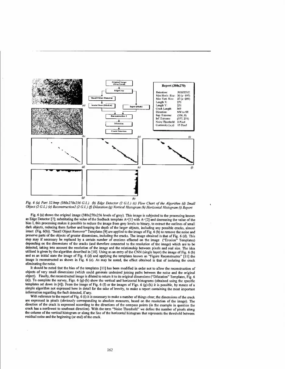
1 Oririn.llraanc | (Gray LmnJ)

I

r^ EdBFOrny -

1 SniUOMMRoor« 1

1 I*p«t (Muk) 1

1 ~^l J~~ c RaconKrortJon 2

i c Dilatation

i c Crack Ditettian

Report (380x270)

Detection: POSITIVE Max Horiz. Size: 30(y=197) Max Vert. Size: 27(x-289) Length X: 271 Length Y: 251 Crack Length: 369 Direction: NWtoSE Sup. Extreme: (106,0) Inf. Extreme: (377,251) Noise Threshold: 2 Pixel Continuity (x,y): 15 Pixel

V

<c)

(d) ~w^*n**m (<)

<*> fit Fig. 6 (a) Part 32.bmp (380x270x256 G.L.) (b) Edge Detector (2 G.L.) (c) Flow Chart of the Algorithm (d) Small Object (2 G.L.) (e) Reconstruction (2 G.L.) (f) Dilatation (g) Vertical Histogram (h) Horizontal Histogram (i) Report

Fig. 6 (a) shows the original image (380x270x256 levels of grey). This image is subjected to the processing known as Edge Detector [7]; substituting the value of the feedback template A=[l] with A=[2] and decreasing the value of the bias I, this processing makes it possible to reduce the image from grey levels to binary, to extract the outlines of small dark objects, reducing them further and keeping the depth of the larger objects, including any possible cracks, almost intact (Fig. 6(b)). "Small Object Remover" Templates [9] are applied to the image of Fig. 6 (b) to remove the noise and preserve parts of the objects of greater dimensions, including the cracks. The image obtained is that of Fig. 6 (d). This step may if necessary be replaced by a certain number of erosions effected on the image ("Erosion" Templates) depending on the dimensions of the cracks (and therefore connected to the resolution of the image) which are to be detected, taking into account the resolution of the image and the relationship between pixels and real size. The idea utilised is given by the algorithm described in [10]. Using as an entry of the CNN (single layer) the image of Fig. 6 (b) and as an initial state the image of Fig. 6 (d) and applying the templates known as "Figure Reconstructor" [11] the image is reconstructed as shown in Fig. 6 (e). As may be noted, the effect obtained is that of isolating the crack eliminating the noise.

It should be noted that the bias of the templates [11] has been modified in order not to allow the reconstruction of objects of very small dimensions (which could generate undesired joining paths between the noise and the original object). Finally, the reconstructed image is dilated to return it to its original dimensions ("Dilatation" Templates, Fig. 6 (e)). To complete the survey, Figs. 6 (g)-(h) show the vertical and horizontal histograms (obtained using the specific templates set down in [4]). From the image of Fig. 6 (f) or the images of Figs. 6 (g)-(h) it is possible, by means of a simple algorithm not expressed here in detail for the sake of brevity, to make a report containing the most important information regarding the fault detected, if any.

With reference to the report of Fig. 6 (i) it is necessary to make a number of things clear; the dimensions of the crack are expressed in pixels (obviously corresponding to absolute measures, based on the resolution of the image). The direction of the crack is expressed according to the directions of the compass points (in the example in question the crack has a northwest to southeast direction). With the term "Noise Threshold" we define the number of pixels along the column of the vertical histogram or along the line of the horizontal histogram that represents the threshold between residual noise and the beginning (or end) of the crack.

162

Fig. 7 Algorithm for the Detection of cracks for images with varying characteristics of luminosity

With the term "Continuity" we refer to the maximum number of white pixels, calculated along the final column of the vertical histogram or along the first line of the horizontal histogram for which the crack is understood to be interrupted. Moreover a threshold of minimum length is established for which ah isolated object may effectively be considered a crack. The aforementioned thresholds are chosen on the basis of experience, both the resolution of the image and the minimum dimension of the object to be extracted being known. Finally, Fig. 7 shows an algorithm which may be adapted to different types of image similar to those used as samples in this study. The adaptation of the algorithm is based on the calculation of the B/W ratio between black and white pixels present in the image obtained from the original with the application to this image of "Average" templates [2]. Fig. 8 shows the table containing the results obtained by applying the algorithm described in Fig. 7 to images acquired with different types of luminosity. The tests were carried out on 100 images, 75 of which contained faults. It may be noted that 100% of the cracks were detected and a false alarm was raised in only one case.

163

TESTS CARRIED OUT

Total number of images 100 Number of images with Cracks 75 Cracks Detected 75 False Alarms 1 Correct length of Crack (within 20%) 72 Incorrect length of Crack (over 20%) 4 Correct position of Crack 72 Incorrect position of Crack 4 Noise Threshold 3 Crack Continuity Threshold Depending on Dimensions of the image

Fig. 8 Table of tests carried out on the images examined

5. Conclusions and Future developments

The present study offers some methodologies based on CNN's for the non-destructive checking of mechanical parts by means of image processing. Most of the algorithms implementing the techniques described use templates known in literature, sometimes modified or adapted to the type of problem under study. This work is conceived as a preUminary phase to the implementation of an automatic system capable of detecting and characterising faults which may be present in mechanical parts in order to exonerate human resources from these tasks and to optimise timing and costs of the checking procedure. Future developments will start from the results obtained in the present study and bear in mind the previous experiences in the field of quality control based on CNN [12] and on neural techniques [1],[13], in order to study the possibilities of implementing hybrid structures combining CNN's for low-level vision (pre-processing and segmentation), artificial neural networks for higher-level operations (recognition and description) and stereoscopy (calculation of the depth of the crack), which would make it possible to effect checking operations in the field of all three dimensions.

References

[I] Fargione G., Geraci A. L., Pennisi L. and Risitano A., "Development of an Algorithm for the Analysis of Surface Defects in Mechanical Elements", Proceedings of SPIE International Symposium on Intelligent Systems and Advanced Manufacturing Conference pp. 374-384,, Boston, USA 1998.

[2] Chua L. O. and Yang L., Cellular Neural Networks: Theory. IEEE Transactions on Circuits and Systems Vol 35 No. 10, October 1988, pp. 1257-1272.

[3] Chua L. O. and Yang L., Cellular Neural Networks: Applications. IEEE Transactions on Circuits and Systems Vol. 35 No. 10, October 1988, pp. 1273-1290.

[4] Chua L. O. and Roska T., The CNN Paradigm" IEEE Transactions on Circuits and Systems Vol. 40 No. 3, March 1993, pp. 147-156.

[5] Crounse K. R, Roska T., and Chua L. O., "Image Halftoning with Cellular Neural Networks", IEEE Transactions on Circuits and Systems-II: Analog and Digital Signal Processing, Vol. 40, No. 4, pp. 267-283, 1993.

[6] Roska T., Kek L., Nemes L., Zarandy A. and Szolgay P., CSL CNN Software Library (Templates and Algorithms) Vers. 7.3, Budapest, Hungary, pp. 39-42, August 1999.

[7] Roska T., Kek L., Nemes L., Zarandy A and Szolgay P., CSL CNN Software Library (Templates and Algorithms) Vers. 7.3, Budapest, Hungary, p. 23, August 1999.

[8] Bertucco L., Nunnari G, A Multi-Layer Cellular Neural Network Simulator for Image Processing Applications, Proceedings of the third International ICSC Symposia on Intelligent Industrial Automation IIA'99 and Soft Computing SOCO'99, pp. 147-151, June 1999, Genova, Italy.

[9] Zarandy A, Werblin F., Roska T. and Chua L. O., "Novel Types of Analogic CNN Algorithms for Recognizing Bank-Notes", Proceedings of the International Workshop on Cellular Neural Networks and Their Applications (CNNA-94), pp. 273-278, Rome, 1994.

[10] Roska T., Kek L., Nemes L„ Zarandy A and Szolgay P., CSL CNN Software Library (Templates and Algorithms) Vers. 7.3, Budapest, Hungary, pp. 114-116, August 1999.

[II] Roska T., Kek L., Nemes L., Zarandy A. and Szolgay P., CSL CNN Software Library (Templates and Algorithms) Vers. 7.3, Budapest, Hungary, p. 28, August 1999.

[12] Bertucco L., Nunnari G, Quality Control Through Image Processing: New Opportunity Offered by CNNs, Proceedings of the third International ICSC Symposia on Intelligent Industrial Automation IIA'99 and Soft Computing SOCO'99, pp. 396-402, June 1999, Genova, Italy.

[13] Catania A, Fargione G, Geraci A and Russo F., "Development of a Neural Network Hybryd for the Analysis of Surface Defects in Mechanical Elements", Proceedings of International Conference on Design Tools and Methods in Industrial Engineering, Associazione Nazionale Disegno di Macchime, Firenze, Italy, 1997.

164

2000 6™ IEEE Internationa] Workshop on Cellular Neural Networks and Their Applications Proceedings

A Qualitative Model-Framework for Spatio-temporal Effects in Vertebrate Retinas

D. Bälya**, B. Roska*, E. Nemeth, T. Roska*, F. Werblin

♦Analogical & Neural Computing Laboratory, Computer and Automation Research Institute, Lägymänyosi u. 11, Budapest, H-l 111, Hungary

phone: 36 1 2095357 e-mail: balya@sztaki.hu

■"Vision Research Laboratory, Department of Molecular and Cell Biology University of California at Berkeley, Berkeley, CA-94720, USA

ABSTRACT: Retinal models based on the Cellular Neural Network (CNN) paradigm [2] have been widely used [3-8]. These neuromorphic models are based on retinal anatomy and physiology [1, 10-11]. In this paper a framework is proposed for qualitative spatio- temporal studies in vertebrate retinas. The underlying retinal anatomy is followed as closely as possible, the characteristics of the physiological models, however, are kept simple. The goal is to model the qualitative effects. Since the developed models are simple, compared to a fully neuromorphic one [9], we have a good chance to implement them on CNN Universal Machine chips [12, 13] using multi-layer technology [14].

1. Introduction

This paper presents a Cellular Neural Network (CNN) [2] model framework for the whole light-adapted rabbit retina. The developed models can reproduce many measured features of the retina. The modeling approach is neuromorphic in its spirit, relying on both morphological and electrophysiological information. The primary motivation lies in fitting the spatial and temporal output of the model to the data recorded from biological cells (tiger salamander and rabbit). In order to maintain a low complexity (VLSI) implementation [13], some structural simplifications have been made while large neighborhood interaction and inter-layer signal propagation are modeled through diffusion and wave phenomena.

Our goal is to develop a CNN based functional vertebrate retina model. The model should produce results qualitatively similar to the living vertebrate retina measurements. The structure of the model can be based on our knowledge about the retinal morphology. The CNN paradigm provides the basic structure and connections for the modeling [12], because CNN has a retina-like structure it is the straightforward to map from the biologic cell layers to CNN layers [3].

We will not try to model all cell layers of different types, just the functionally important ones. We will not use the measurement results directly, moreover we do not aim to create operationally complete and exact cell models [9]. Our goal is less ambitious: we try to develop a simple model using correct cell, layer and structure properties and we settle for qualitatively correct results. Our full vertebrate retina model, however, is able to reproduce many of the main retinal phenomena, parallel.

A further goal is to understand the connection between structure and function of the retina [7], The living vertebrate retina has a complicated structure and performs sophisticated operations with several different building blocks. The goal of the simplification is not to copy all of the conditions of the measurement, but create a rather simple model for calculating the primary retina transformation of the natural scenes or artificial stimulation without second order additional effects, such as e.g. contrast-adaptation.

Our CNN "retina", as a computational device, is a complex and sophisticated tool for preprocessing a video flow [5]. It may be used in several algorithms and applications. Using a retina transformation we are able to develop an efficient algorithm for several types of tracking, classification and recognition tasks.

2. The general framework

Receptive Field Interaction (abbreviated RFI) Prototypes are used in an experimental simulation framework for elementary spatio-temporal phenomena in the retina. The receptive field prototypes, the synapse prototypes, and the layer prototypes are preprogrammed so that, only a few parameters are controllable. With these prototypes the RFI schema is composed. The Receptive Field Interaction Schemas are studied under various inputs at various parameters to develop appropriate vertebrate retina models.

0-7803-6344-2/00/$10.00 ©2000 IEEE 165

2.1 Cell (and Layer) Prototypes

Cl: First order

(JXjl — _ Xji + ■*!/ V

Aijkiykl ■ Bijki"k! ■ \k-i\<r,\l-j\<r \k-i\<r\l-j\<r \k-i\<r\l-j\<r

\xu+i~\xu~i yij = n*ij)=——^—L; \<,i<MMj<N

Dijki^(yki>xki^ki) + Iij

(Cl)

The required parameters are • z, the bias or resting potential

• T, the time constant is determined by the linear capacitor and the resistor and it can be expressed as t = AC • A, the feedback template(s) or synapse(s) and the D matrix or matrices

C2: Simple second order It is the same as the Cl type except for an additional capacitance connected across the output of the cell. The

second time constant is an additional parameter.

2.2 Synapse Types

The following functions are multiplied by the weight parameters of the receptive field. Transfer function

Linear bipolar

Saturated bipolar

It represents linear "electrical" synapses or simple signal transfers.

It represents saturated linear synapses, e.g. chemical transfers.

/(*) = *

f(x) = '/2{\x+l\-\x.)\)

(SI a)

(Sib)

Simple rectifier

Linear rectifier

Exponential rectifier

It models a simple nonlinear transfer function.

It models one kind of nonlinear transfer function.

It is an advanced non-linear rectifier.

/« = 'x>(

:0:0

'x>0:x

f x < cx : cy

/MHX>C .(^-Qx + fa-c,) f-c,.-

2

c,-l

/(*) = l + e -c(*-l)

(S2a)

(S2b)

(S2c)

Sigmoid It represents a continuos synapses, ftx\ = 2C

stand for non-linear dependence on ^i + e"c>'»i-(-<"c-«) 2

the presynaptic voltage. + c

1 n (S3)

It defines a voltage-controlled ion VCCtemplate channel (generally used for f(xs,xd) = fsigm0id(x5)(Er-xd) (54)

modeling neurons).

2.3 Receptive Field Types

RFO: Simple central gain: This is a simple feed-forward receptive field. The strength of the coupling is the gain value.

RF1: Gaussian-type This type of spatial weighting can be used for chemical synapses describing both the intra-layer and inter-

layer interactions.

GO/2) G0) G(V2) G(l) G(0) G(I)

GfV2) GO) G(V2) G(x) = Ne''*""2 and G(0)+4(G( 1)+ G(V2)) = 1

(RF1)

166

RF2: Diffusion-type This type of spatial weighting can be used to describe the intra-layer diffusion-type phenomena. The cells in

layers are tightly coupled. The space constant (X) is an appropriate value to determine the strength of coupling. This is an A template.

(RF2a)

(RF2b) V73 X2/3 A/73 X2B -8 X2B X2/3 g or

X2B X2B X2/3

X/2 X X/2 X -6X X

X/2 X X/2

RF3: Center-surround structure This symmetric template can be used for both ONcenter-OFFsurround or OFFcenter-ONsurround structures.

RF4: Pattern defined Each weight in the matrix is adjustable.

2.4 Visual Input

VII: Still image The static image means, that the image (e.g. white square) is shown to the retina on a gray background for a

defined time interval and after that the stimulus becomes a blank gray field. Still means the image is shown for a time span and after that the visual input is a gray field. The adjustable parameters are: the on-time when the input is the static image, the off-time when the visual input is a gray field.

VI2: Video During the video stimulus a video-flow is projected to the retina. A frame is shown constantly till the next

frame appears. The video speed is 30 frame per second, and the typical total time is some seconds. The basic video stimuli are the moving ball in different directions and the increasing square.

3. The qualitative retina modeling framework

Our model building approach is to incorporate the available knowledge on morphology, electro-physiology and pharmacology. The starting-point of the model is the living retina, with properties derived from the vertebrate retina measurements [10]. The biological terms can correspond to the following CNN terms [4]. A CNN cell models a biological cell, one specific type of biological cell is modeled with a CNN layer and the synapses (inter and infra layer, excitatory, inhibitory as well) are transformed to the CNN template.

The input of the retina is activation of the cone (photoreceptor) layer and the output is the ganglion cell spiking. In the modeling we use analog output for the description of the state of every cell. It is reasonable for the ganglion cells, too, because the spiking is considered as one type of analog signal representation [6]. The outputs of the different cell layers are transformed to grayscale video. Pixels in each video frame correspond to individual cells and color of the point indicates the voltage of the cell. In this modeling each layer is working on a predefined interval (-1,1) and not in the measurement value-space. By using this constraint, relations of layers to each other can be easily compared in simulations. The qualitative behavior of the layer (or model) is graphic. The modeling is easier to perform and to overview.

The modeling takes the following steps. First, the model structure is defined, the layers and synapses are created. Second, the model parameters are defined: the time constant for each layer and the transfer function and the receptive field for each synapse. Third, the stimulus is selected (e.g. the same stimulus is used as in the measurement) and the simulation begins.

The model framework has the following restrictions: • In the retina just the cone (and rod) cells are able to transform the light to electrical signal, hence in the

modeling, the stimulus is the input (has a non-negative B template) just for one layer. • A layer contains first or simple second order cells. Almost every cell type has a non-linear higher order

transfer function; it can be modeled as a first or second order system [5]. • The cell delay is continuous. The cells are working in analog mode. • The steady state voltage of a cell can be calculated from the state equation of the biological cell. In the

modeling we set this voltage to zero. The model conserves the basic property of the behavior, but the computation is much easier.

• The applied CNN templates are space-invariant and use the nearest neighborhood. The different types of cells have different size of interactions. This bigger field can be modeled with a diffusion feedback (RF2).

167

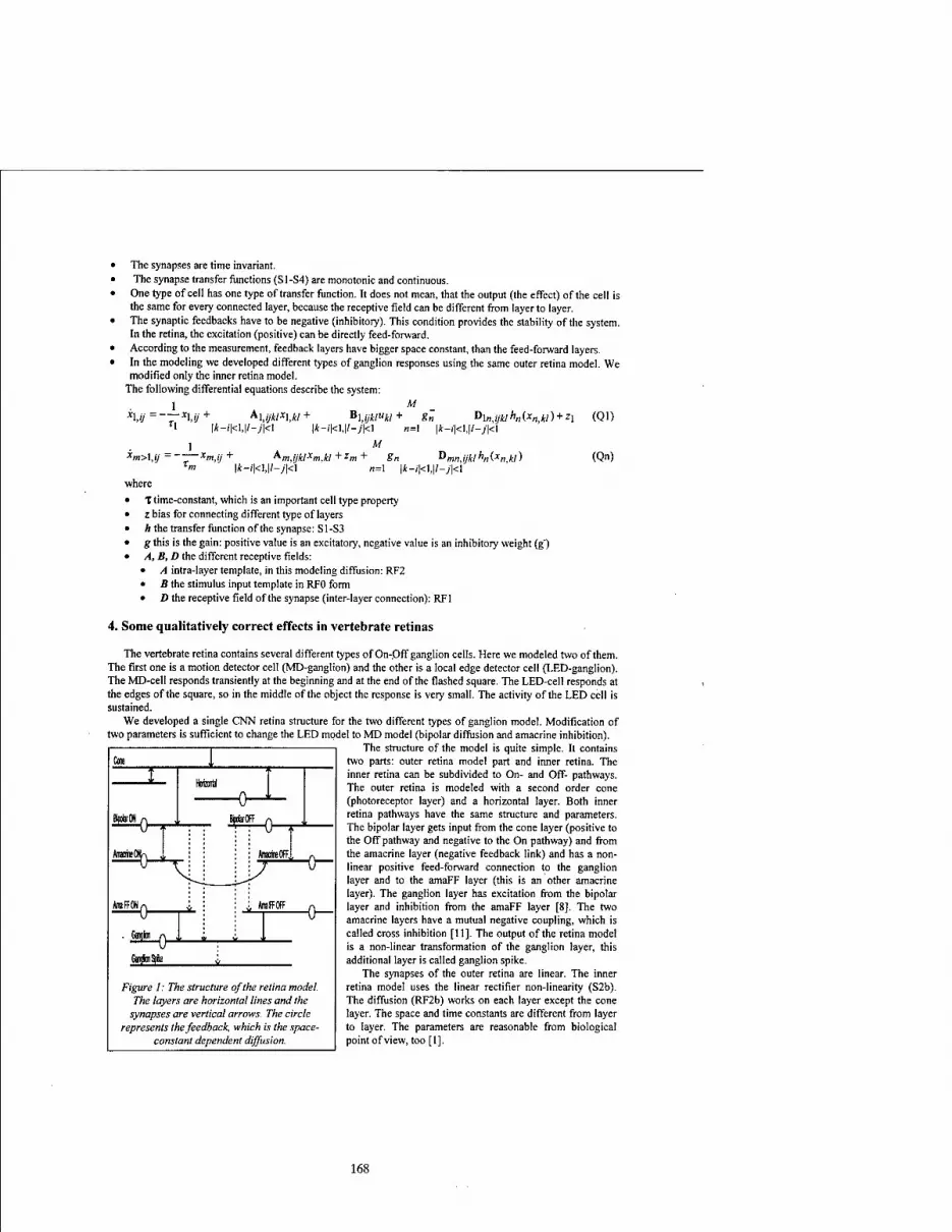
The synapses are time invariant. The synapse transfer functions (S1-S4) are monotonic and continuous.

One type of cell has one type of transfer function. It does not mean, that the output (the effect) of the cell is the same for every connected layer, because the receptive field can be different from layer to layer. The synaptic feedbacks have to be negative (inhibitory). This condition provides the stability of the system. In the retina, the excitation (positive) can be directly feed-forward. According to the measurement, feedback layers have bigger space constant, than the feed-forward layers. In the modeling we developed different types of ganglion responses using the same outer retina model. We modified only the inner retina model.

The following differential equations describe the system: 1 M

*\,ij=-—x\,ij+ M,ijkl*\,kl + Bl,(yW«W+ gn Dln,iyW *«(*«,«)+ zi (Ql) |*-i|<l,|/-y|<l |*-;|<i,K-;|<i n=l |i-i|<l,|/-y|<l

xm>\,ij

where

Am,ij I*-

^■m,ijklxmikl *zrr, M

n=l |i-/|<l,|/-y|<l i,ijklhn(xn,kl) (On)

T time-constant, which is an important cell type property z bias for connecting different type of layers h the transfer function of the synapse: S1-S3 g this is the gain: positive value is an excitatory, negative value is an inhibitory weight (g') A, B, D the different receptive fields:

• A intra-layer template, in this modeling diffusion: RF2 • B the stimulus input template in RFO form • D the receptive field of the synapse (inter-layer connection): RF1

4. Some qualitatively correct effects in vertebrate retinas

The vertebrate retina contains several different types of On-.Off ganglion cells. Here we modeled two of them. The first one is a motion detector cell (MD-ganglion) and the other is a local edge detector cell (LED-ganglion). The MD-cell responds transiently at the beginning and at the end of the flashed square. The LED-cell responds at the edges of the square, so in the middle of the object the response is very small. The activity of the LED cell is sustained.

We developed a single CNN retina structure for the two different types of ganglion model. Modification of two parameters is sufficient to change the LED model to MD model (bipolar diffusion and amacrine inhibition).

The structure of the model is quite simple. It contains two parts: outer retina model part and inner retina. The inner retina can be subdivided to On- and Off- pathways. The outer retina is modeled with a second order cone (photoreceptor layer) and a horizontal layer. Both inner retina pathways have the same structure and parameters. The bipolar layer gets input from the cone layer (positive to the Off pathway and negative to the On pathway) and from the amacrine layer (negative feedback link) and has a non- linear positive feed-forward connection to the ganglion layer and to the amaFF layer (this is an other amacrine layer). The ganglion layer has excitation from the bipolar layer and inhibition from the amaFF layer [8]. The two amacrine layers have a mutual negative coupling, which is called cross inhibition [11]. The output of the retina model is a non-linear transformation of the ganglion layer, this additional layer is called ganglion spike.

The synapses of the outer retina are linear. The inner retina model uses the linear rectifier non-linearity (S2b). The diffusion (RF2b) works on each layer except the cone layer. The space and time constants are different from layer to layer. The parameters are reasonable from biological point of view, too [1].

Figure I: The structure of the retina model. The layers are horizontal lines and the

synapses are vertical arrows. The circle represents the feedback, which is the space-

constant dependent diffusion.

168

The following two tables show the comparison of the three examined simulations and measurements. The model reproduces the basic features of the desired retina effects. One model (structure and parameters) is able to reproduce the qualitatively correct response for this three stimuli

LED Measurement LED Simulation Properties

f I On stimulus (time: 1+lsec, size: 60pixels) Basic: activity only at the edges

Further properlies: • strong initial answer • while stimulus on, strong outside edge • after stimulus strong inside edge

1000 2000 3000 «5 low 2Soa sowwa Moving ball (speed in ujm/sec) Basic: bigger speed smaller response

Further properties: • Off response is weak » Exponential envelope

J a»

Incremental square (size in um) Basic: bigger size smaller response

Further properties: • Long time activity • Exponential envelope

Table 1: The examination of the Local Edge Detector Ganglion Model

MD Measurement MD Simulation Properties

■s\i

466 )666 2656 MM 68811

L_U

On stimulus (time: 1+lsec, size: 60pixels) Basic: Response just at the beginning and

at the end of the stimulus

Further properties: • strong response at the beginning » sometimes longer response near the edges

400 1000 2000 3000 6000

lUL itliLtlMi

Moving ball (speed in um/sec) Basic: big response to middle square

Further properties: • Off response is weak • Gauss envelope

50 100 200 400 1000 100 200 4ÖÖ1000

JL

Incremental square (size in \im) Basic: big response to middle square

Further properties: • Gauss envelope » Different On and Off response

Table 2: The examination of the Motion Detector Ganglion Model

The first measurement is in response to the basic On stimulus. A white square is shown for a second and a blank gray background during the next second. On the picture the time is on the vertical axes and the middle row of the retina is the horizontal axes.

The second stimulus is the moving ball. A white circle is moving towards the right side of the retina with different speed and the measurement is on the middle cell. The relationship between the speed and the grade of the response is the task. The horizontal axes is the time, the vertical is the response. The number above the curves indicates the speed of the object in micron per sec.

The third measurement is the growing square. A white square is shown to the retina. The connection between the size of the object and the grade of the response is the question. The horizontal axes is the time, the vertical is

169

the response. The number above the curves indicates the size in micron. In the simulation one pixel is 30 micron, this is an acceptable map according to the density of the cone cell in a general vertebrate retina.

5. Acknowledgement This work was supported by the ONR N68171-97-C-9038, OTKA T026555 and the Hungarian Academy of

Sciences.

6. Conclusions

The proposed model is a framework for CNN retinal models: it provides a new simulation platform for creating retinal model with biologically relevant parameters. We developed a CNN structure and parameters (prototypes) for modeling the vertebrate retina from photoreceptors to ganglion cells. The implemented two basic ganglion cell models (motion and edge detector) have the same structure and we can switch between them using two key parameters, namely the bipolar diffusion and amacrine inhibition. The abstraction level of the model is not as low as the CNN core or a complex cell with ion channels and not as high as some special neuron simulator or abstract mathematical transfer function, it uses qualitatively important and biologically relevant parameters and retina-morphic structure. We could compute the retinal transformation of any video sequence.

The outputs of our CNN model for some simple inputs are very similar to the outputs of the vertebrate retina. The examined stimuli and the reproduced retina effects were:

• Flashed square: the output is the space or the time edge of the square • Increasing square: the output depends on the size of the object • Moving spot: the output depends on the speed of the moving spot

These effects may be useful for image processing tasks such as: • edge and object corner detection in space and time • object level motion detection with size selectivity (beside local interactions) • speed, size and intensity selective video-flow processing with impulse noise filtering in space and time

7. References

[I] F. S.Werblin: "Synaptic connections, receptive fields, and patterns of activity in the tiger salamander retina", Investigative Ophthalmology and Visual Science, Vol. 32, pp. 459-483, 1991 [2] L. O. Chua and L. Yang: "Cellular Neural Networks: Theory", IEEE Trans, on Circuits and Systems, Vol. 35, pp.1257-1290, 1988 [3] F. Werblin, T. Roska and L. O. Chua: "The analogic cellular neural network as a bionic eye", Intl. Journal of Circuit Theory and Applications, Vol. 23, pp. 541-569, 1995 [4] T. Roska, J. Hämori, E. Läbos, K. Lotz, L. Orzo, J. Takäcs, P. L. Venetiäner, Z. Vidnyänszky, and Ä. Zarändy: "The Use of CNN Models in the Subcortical Visual Pathway", IEEE Trans, on Circuits and Systems-I: Fundamental Theory and Applications, Vol. 40, No. 3, pp. 182-195, March 1993. [5] A. Jacobs, F. Werblin: "CNN-based retinal model uncovers a new form of edge enhancement in biological visual processing", Proc. of CNNA-96, Seville, Spain pp.303-307,1996 [6] F. Werblin, A. Jacobs: "Using CNN to unravel space-time processing in the vertebrate retina", Proc. of CNNA-94, Rome, Italy, pp.33-40, 1994 [7] A. Jacobs, T. Roska and F. Werblin: "Methods for constructing physiologically motivated neuromorphic models inCNNs", International Journal of circuit theory and applications, 24, pp. 315-339, 1996 [8] F. S. Werblin and D. R. Coppenhagen: "Control of Retinal Sensitivity: III. Lateral Interactions at the Inner Plexiform Layer", Journal Gen. Physiology, Vol. 63, pp. 88-110, 1974 [9] Cs. Rekeczky, T. Roska, B. Roska, E. Nemeth, F. Werblin: "Neuromorphic CNN models for spatio-temporal effects measured in the inner and outer retina of tiger salamander", Proc. IEEE CNNA-2000, Catania, 2000 [10] B. Roska, E. Nemeth, L. Orzo, F. Werblin: "Three Levels of Lateral Inhibition: A Space-time Study of the Retina of the Tiger Salamander", Journal of Neuroscience Vol. 20(5): pp.1941-1951, 2000 [II] B. Roska, Nemeth E, Werblin F.: "Response to change is facilitated by a three-neuron disinhibitory pathway in the tiger salamander retina", Journal of Neuroscience Vol. 18(9): pp.3451-3459,1998 [12] T. Roska and L. O. Chua: "The CNN universal machine: an analogic array computer", IEEE Trans, on Circuits and Systems II, Vol. 40, pp. 163-173, 1993 [13] S. Espejo, R. Dominguez-Castro, G. Lilian, Ä. Rodriguez-Vazquez, "A 64x64 CNN Universal Chip with Analog and Digital I/O", in Proc. of 5th Int. Conf. on Electronics, CAS ICECS'98, pp. 203-206, Lisbon, 1998 [14] T. Serrano, Cs. Rekeczky, Ä. Rodriguez-Vazquez, and T. Roska "A stored program 2nd order / 3-layer complex cell CNN-UM", Proc. IEEE CNNA-2000, Catania, 2000

170

2000 6™ IEEE International Workshop on Cellular Neural Networks and Their Applications Proceedings

Cellular Neural Networks with nearly arbitrary nonlinear weight functions

A. Loncar and R. Tetzlaff

Institut für Angewandte Physik, Universität Frankfurt Robert Mayer-Straße 2-i, 60054 Frankfurt a. M., Germany

phone: +49 69 798 28317, fax: +49 69 798 28865 e-mail: A.Loncar@iap.uni-frankfurt.de

ABSTRACT: In this paper we present Cellular Neural Networks (CNN) with a new type of nonlinear weight functions. Instead of representing a weight function by a n-th order polynom [1], we propose tabulated functions by using a cubic spline inter- polation procedure. These CNN are considered for the problem of modelling nonlinear systems, which are characterized by partial differential equations (PDE). Therefore we propose a training algorithm to adjust the behaviour of CNN solutions to the solutions of a given nonlinear system. Results are given for the ^-equation and the achieved accuracy is compared to the approximation accuracy of solutions obtained by a direct spatial discretization of the $4 -equation.

1. Introduction

During the past few years the dynamics of CNN [2, 3] were studied in an increasing number of investigations, e.g. in order to model nonlinear systems. In this contribution the modelling of autonomous spatio-temporal systems by having only a rough knowledge about the underlying PDE is considered. The autonomous case is treated without loss of generality, because the modelling problem can easily be generalized to any kind of CNN. The dynamic behaviour of an autonomous multi-layer CNN can be represented by state equations of the form

where «f' (t) represents the state of cell i in layer m!. ff™'m(r) is the set of cells in a layer m' that are neighbours of cell i in a layer m. The connection from a cell i + j in layer w! towards a cell i in layer m is denned by the weight function ag}.'™, which depends on a vector j?j+™ of adjustable parameters. The cell output is not considered explicitely in (1), because it can be included in the definition of the weight function according to

^"(«ÄW.flt") = <"(/«*Kfi(*)).inkm)- Since the state equations of CNN form a system of locally interconnected nonlinear ordinary differential

equations, the dynamics of a nonlinear system can be represented by the cell dynamics of a CNN [4]. If a CNN and a nonlinear system are initialized with the same initial condition, they will generally show a different dynamical behaviour, as demonstrated in Fig. 1. In order to obtain an accurate CNN model a training algorithm has to be applied for a correct determination of the CNN weight functions.

In earlier investigations [1, 3] we have represented nonlinear systems with spatio-temporal solutions by CNN with polynomial weight functions. In certain cases a high polynomial order up to 40th order is necessary, which may result in numerical instabilities, especially during the parameter training. In order to overcome this problem we propose tabulated weight functions by using a cubic spline interpolation [5].

It is well known [6], that a cubic spline interpolation formula is smooth in the first and continuous in the second derivative. To obtain a unique solution for a cubic spline K pair of values (u|+^*>a$+j"(Uj+£*)) of a tabulated function and the first derivatives at its boundaries a'£™(u^j1),a'.£-m(u'Z^jK) are required for each weight function, leading to a parameter vector

~m'm Ia-fm' „m'm{~m' \ „im'm(.,m' \ ntm'm(n.m' \\ (i)\ Pi+j -{ui+j,ai+j (ui+j),ai+j (ui+li),ai+j (ui+jtK)). (Z)

0-7803-6344-2/00/$10.00 ©2000 IEEE 171

time trajectory of a " ear system

CNN-trajectory Tv after a parameter,/ training

"initial cöhditiö;

<T CNN-trajectory before a parameter training

CNN output space

Figure 1: The modelling problem.

2. Parameter training

For the parameter determination we assume S training patterns to be known. Each training pattern consists of two solutions Uj"(t,,o) and Uj"(t8ii) at times tsß and tSii with t,?i > t,,o of a nonlinear system to be modelled . The values u5"(t,,o) are taken as the initial cell states u^(tS|0) of the CNN model with the parameter vector p, that contains all elements p™ J™ according to (2). At tti\

M . N

m—1 i—1 (3)

is calculated, where «5"(t»,i,p) represents the cell states of the CNN model at t,,i. Then p will be determined by a minimization of the mean square error (MSE)

E(a=-si>(».fl (4)

for all training patterns. We used Powell's method [7] for the minimization of the MSE which requires no explicit gradient information. The values a?£j'(iiQj),a'g'j

m(u?£jil),a'%'jm(u'tf.j:K) are initialized with

gaussian random values, whereas u™ j- will be taken according to

A< = ma,(2|„r-(t)|) ^

U&-, = -max(\y?(t)|) and u^k = u^it_, + A«^- V* = 2,3,..., K.

3. The $4-equation

In order to study the performance of the training procedure we considered a nonlinear system described by the $4-equation

d2u(x, t) d2u(x,t) ,, ,. ... ,.,

where the long term behaviour of a solution could be highly sensitive to the chosen initial state. Typical examples are the kink-antikink collisions, which are defined by kink solutions

u+(x,t)=tanhl x-v+t~xZ

and antikink solutions

u (x,t) = —tank

v/2(i - (v+y)

X — V~t — XQ

V2(l - (v-)2)

172

100

64 o

100

6<r~o -Figure 2: Kink-antikink collision with v = 0.190. Figure 3: Kink-antikink collision with v = 0.192.

100

64 o

Figure 4-' Kink-antikink collision with v = 0.200.

i i+1 i+2 .... ^y .... m=2

Figure 5: CNN model.

The initial cell states are then obtained according to

u(x,0) = u+(x,0) for x<^. Xn T" Xn

u-(s,0) for x>X° ~tX~°

with xj = 24 and x0 = 40. Depending on the velocities v+ and v~ the solutions of the kink-antikink collisions show, as illustrated in Fig. 2-4, a complete different behaviour for a slightly changed velocity V = v+ = v~.

4. Results

For modelling the dynamic behaviour of a nonlinear system described by the *4-equation we considered autonomous CNN, which are shown in Fig. 5. The weight functions of the CNN model are defined by tabulated functions using cubic spline interpolation with K = 2 sampling points. Since the state equations of a CNN form a system of coupled ordinary differential equations (ODE), the solutions of a given PDE can be approximated by the CNN output values. Therefore a spatial discretization of (5) with stepsize Ax leads to a set of ODE [8], which has to be identified by the set of state equations (1). In order to study the effect of spatial discretization we have calculated solutions of (5) numerically with Ax = 1/32 for a CNN

173

LU tn s

0.1

0.01

0.001

0.0001

1e-05

16-06 •

1e-07

1e-08 10 15 20 25

number of trainingsteps [-10 ]

Figure 6: MSB vs. number of trainingsteps.

with N = 2048 cells. Then every fourth value of the obtained solutions has been taken to form a training pattern for a CNN model with N = 512 cells which corresponds to a stepsize Ax = 1/8. The solutions for v = 0.200 given in Table 1 have been taken as the training patterns. Thereby, by minimizing the

name time range of values of the training pattern

r«,0 *s,l m = l (u(i,t)) m = 2 (v(x,t)) Tpl 75.0 75.5 [-1.0172,0.9958] [-0.0331,0.1258]

TpS 33.0 33.5 [_l.4468, -0.7750] [-1.3390,0.0000] TpS 33.5 34.5 [-1.6588, -1.0000] [-1.1337,1.2831]

Table I: Training patterns with v = 0.200.

MSE (4) only certain training patterns Tpl-3 will be considered in a single step of the training procedure. Our investigations showed that a three-step training algorithm always leads to the best performance in the error minimization. A scheme of the applied training algorithm is given in Table 2.

presented training pattern 1st step 2nd step 3rd step

Tpl Tpl,Tp2 Tpl,Tp3

Table 2: Scheme of the three step training algorithm

The performance of the error minimization is shown in Fig. 6. We evaluated the achieved modelling accuracy by calculating the deviations of certain solutions of the trained CNN model (CNNj/h with Ax = 1/8, N = 512) to reference solutions obtained by a direct spatial discretization (CNNfi32 with Ax = 1/32, N = 2048) of (5). Therefore the root relative mean square error (RRMSE)

Er(p) =

\

^2(ui/s(x,t) -ir1/32(x,r))2

(6)

5^«l/32(*.')2

has been considered for t = [0,100] with At = 0.5, where

Ui/s(x,t) = {ui/s(xut),u1/s(x2,t),...,u1/s(x5i2,t)} and

«1/32 OM) = {u\/32(xi,t),Ui/32{x!j,t),...,Ui/a{x20Vi,t)};

here Xi denotes the cell position. Additionally, the solutions u1/32(x,t) have been compared to those obtained by a spatial discretization of (5) with Ax = 1/8 and N = 512 (CNN°/g). The RRMSE are shown in Table 3.

174

CNN model Erip) v+ = v- = 0.190 v+ = v- = 0.192 v+ =v- = 0.200

CNN[/S 8.51 • 10"2 3.91 • 10-* 8.51 • 10~b

CNNfi, 2.43 • 10-1 2.41 • 10-1 9.99 ■ 10~2

Table 3: RRMSE of CNN?/g and CNNf/s for solutions of the ^-equation.

Au(x,t) Au(x,t)

100

Figure 7: Au{x,t) vs. x and t ofCNNj/s (left) and CNN°/S (right) for v+ =v~ = 0.190

Au(x,t)

100 100

Figure 8: Au(x,t) vs. x and t ofCNNjß (left) and CNN?/S (right) for w+ = v~ = 0.192.

100 100

Figure 9: Au(x,t) vs. x andt ofCNN?/s (left) andCNN^/s (right) for v+ =v~ =0.200.

The results clearly demonstrate the high modelling accuracy of a CNN with tabulated weight func- tions obtained in a training procedure. Especially it follows, that a parameter training leads to more accurate solutions than a direct spatial discretization, which is illustrated in Fig. 7-9 showing the absolute deviations

Au(x,t) = ul/s{x,t)-ui/32{x,t),

where ui/s(x,t) represents the output values of either CWiVJy8 or CNNR^ and Ui/32(i,t) denotes the values of CNN^/32.

175

5. Conclusion

Our results show that a CNN with tabulated weight functions using cubic spline interpolation can be considered for a precise modelling of nonlinear systems. The modelling accuracy is clearly higher than the accuracy of a CNN model obtained by a direct spatial discretization of the underlying PDE, when both CNN models correspond to the same spatial discretization.

6. References

[1] Puffer, F., Tetzlaff, R., and Wolf, D.: "Modeling Nonlinear Systems with Cellular Neural Networks", Proc. ICASSP , Atlanta, pp. 3513-3516, 1996.

[2] Kozek, T., Chua, L.O., Roska, T., Wolf, D., Tetzlaff, R., Puffer, F. and Lotz, K.: "Simulating Nonlinear Waves and Partial Differential Equations via CNN", IEEE Transactions on Circuits and Systems, Vol. 42, pp. 807-820, October 1995.

[3] Puffer, F., Tetzlaff, R., and Wolf, D.: "A Learning Algorithm for the dynamics of CNN with Non- linear Templates - Part II: Continuous-Time Case", Proc. CNNA, Sevilla, pp. 467-72, 1996.

[4] Puffer, F., Tetzlaff, R., and Wolf, D.: "A Learning Algorithm for Solving Nonlinear Partial Differ- ential Equations with Cellular Neural Networks (CNN)", Proc. ISSSE, San Francisco, pp. 501-504, 1995.

[5] Tetzlaff, R., Loncar, A. and Wolf, D.: "Modelling Chaotic Systems by Cellular Neural Networks", Proc. ICNF, Hong Kong, pp. 207-10, 1999.

[6] Greville, T.N.E.: "Theory and Applications of Spline Functions", Academic Press, New York, 1969.

[7] Press, W.H., Flannery, B.P. and Teukolsky, S.A.: "Numerical Recipes in C: The Art of Scientific Computing", Cambridge University Press, New York, 1992

[8] Puffer, F., Tetzlaff, R., and Wolf, D.: "Zur Genauigkeit der mit zeitdiskreten CNN gewonnen Lösungen einiger Differentialgleichungen", Kleinheubacher Berichte, Band 37, Kleinheubach, pp. 245-252, 1993

176

2000 6™ IEEE Internationa] Workshop on Cellular Neural Networks and Their Applications Proceedings

Physical Modeling of RTD-Based CNN Cells

Martin Hänggi, Radu Dogaru, and Leon 0. Chua

Nonlinear Electronics Laboratory University of California at Berkeley

Berkeley, CA 94720 Phone: 510-643-8868 Fax: 510-643-8869

E-mail: haenggiflcomputer. org

ABSTRACT: Resonant tunneling diodes (RTDs) have intriguing properties which make them a primary nanoelectronic device for both analog and digital applications. We present a physics-based model of the RTD and study the universal cell circuit for Boolean CNNs which is proposed in a companion paper [1]. In this circuit, the negative differential resistance of the RTD is fully exploited. Spice simulations confirm that it is capable of realizing a large class of linearly not separable Boolean functions.

1. Introduction

There is a physical limit to how far conventional transistors and integrated circuits can be downscaled. At some point, revolutionary concepts such as nanoelectronics will be needed to meet the challenge of smaller, faster, and better devices and circuits. Nanoelectronics goes back to the mid 1980s,, when work began on resonant tunneling and bandgap engineering in low-dimensional quantum wells and superlattices.

When the size of a system scales down to the size of an electron wavelength, quantum effects take over. When transistors are downscaled and their dimensions are measured in nanometers, new phenomena and devices based on quantum tunneling mechanisms are needed - devices and circuits fabricated with nanometer precision. In the last ten years, advances have been made at realizing artificial semiconductor structures using molecular-beam epitaxy, metal-organic vapor deposition, and chemical-beam epitaxy.

The structural simplicity, the relative ease of fabrication, the inherent high speed, the flexible design freedom, and the versatile circuit functionality make the resonant tunneling diode (RTD) an excellent candidate for nanoelectronics devices in both analog and digital applications. Furthermore, RTDs and FETs can readily be integrated monolithically, allowing extremely compact circuits.

The basic RTD device configuration is a double barrier quantum well structure measured in nanome- ters [2, 3]. The structure has two contacts (the emittor and the collector) made from a semiconductor with a small bandgap (e.g., GaAs), quantum barriers made from a semiconductor with a larger bandgap (e.g., InGaAs), and a quantum well made from the smaller bandgap semiconductor (Fig. 1). The wave nature of electrons in such a structure leads to quantum phenomena like interference, tunneling, and energy quantization; the quantum well is so narrow (ss 5nm) that it can only contain a single, the so- called resonant, energy level. Electrons wishing to travel from the emitter to the collector can only do so if they are lined up with this resonant energy level.

Initially, with a low voltage across the device (point A in Fig. 1), the electrons are below the the point of resonance, and no current can flow through the device. As the voltage increases, the emitter region is warped upwards, and the collector region is warped downwards. Eventually, the band of electrons in the emitter will line up with the resonant energy state, and allows tunneling through to the collector (peak at point B). With higher voltage, the electrons are pushed past the resonant energy level and are unable to continue tunneling, which can be observed by the drop in current to the valley at point C. If the voltage increases further, more and more electrons are able to flow over the top of the quantum barriers, and the current flow will rise.

The negative differential resistance (NDR) between points B and C is the key property of RTDs. In digital applications [4], the NDR property permits compact bistable circuits without feedback. In this paper, however, we focus on the modeling of analog RTD circuits; in particular, we consider the potential of RTDs for the design of uncoupled CNN cells.

While conventional technology requires more than about 60 CMOS transistors to build an uncoupled CNN cell, this number may be reduced by a factor of 3 by using RTDs. Furthermore, the highly nonlinear I—V characteristics of the RTD permits the extension from the linearly separable class of Boolean functions in the standard CNN cell to any Boolean function.

0-7803-6344-2/00/$10.00 ©2000 IEEE 177

quantum baniArs energy / \

Voltage Emitter •

Figure 1: The resonant tunneling diode: I—V characteristics and energy band diagrams.

2. Physics-based Model of Resonant Tunneling Diodes

In order to incorporate the RTD into a Spice-like circuit representation, its current-voltage character- istic has to be modeled with sufficient accuracy. It is desirable to dispose of a model which is based on actual physical parameters such as energy levels, dopant concentrations, and the geometry of the device. In [5], Schulman et al. solved this task satisfactorily, starting by expressing the current density of the RTD with an effective mass approximation,

em'kT

2vr2fi3 / T{E,V) Jo

-In \+e(EF-E)/kT

1+c(Er-£-eV)/*T dE (1)

which includes nonzero temperature and Fermi-Dirac statistics. The transmission coefficient T(E, V) is approximated by a Lorentzian, i.e.,

T(E,V): (W (E-(Er-%)) +(E)2

(2)

where E is the energy measured up from the emitter conduction band edge. ET is the energy of the resonant level relative to the bottom of the well at its center, and F is the resonance width. The formula assumes equal width barriers, which is not always valid. For better generality, eV/2 can be replaced by eVn, with n as a fitting parameter. Calculations show that T is on the order of only one meV even for quite thin barrier widths [6], which is much less than kT at room temperature. The substitution E := Er — eV/2 is therefore resonable, and the integral (1) reduces to

, em'kTT , [1 + e(Er-Er+cv/2)/kT J= ~ ■>.., In

27T2fi3 l+eiEr-Er-cV/2)/kT TV (Er-'-f — + arctan I p—=- )]■ (3)

This formula provides the correct shape of the I—V characteristics, but is calculated in an oversimplified way. The physical quantities can be allowed to deviate from their actual values to compensate for approximations and omissions in the model. The result is of the form

Ji = A In 1 +e(D-C+n,V),/A:T

l + e(B-C-n,V),/*T IT — + arctan mi< (4)

where the parameters A, B, C, and D can, on the one hand, be used to shape the curve to match a measured characteristic, and, on the other hand, have a well-defined physical interpretation. However, (4) merely produces a peak current and an NDR region, but there is no increasing valley current, which is due to tunneling through other channels and inelastic scattering. The simplest way to include a valley current contribution is to give it the form of tunneling through a higher resonance or thermal excitation over a barrier. For voltages below this higher energy channel, the additional current takes on the familiar diode form J2 = H(e™v/kT - 1). The final form of the RTD current density is just the sum J = Jt + J2.

178

Voltage [V]

Figure 2:1—V characteristics of the RTD used in the proposed circuit.

In this paper, we focus on the DC characteristics of the device; hence, the capacitances of the device are neglected. It can, however, be expected that the time constant of the RTD CNN cell will be in the order of tens of picoseconds [2]. For the circuits proposed in this paper, Ji is specified by the parameters A = 4800A/cm2, B = 0.05V, C = 0.07V, D = 0.038V, and ni = 0.2, and an area of 10~8cm2 is assumed. The parallel diode carrying Ji is modeled by a generic Spice diode with an emission coefficient of n = 1.75 and a series resistance of Rs = lkfi (Fig. 2).

The NDR causes RTD circuits to possibly have multiple equilibrium points. Simulators such as Spice, not being explicitly designed for such systems, may encounter problems when solving (dc analysis) or integrating (transient analysis) the network equations [7]. It may therefore be necessary to tune the analysis options of the program in order to get meaningful results.

3. An RTD-Based CNN Cell for Arbitrary Boolean Functions

In all current digital applications of RTDs and in the RTD-based CNN cell circuit presented in [8], the local activity property of the NDR is not really exploited, but merely the bistability property, because the third equilibrium point in the NDR region is not stable in such circuits and therefore unwanted. However, by using the principle of nesting piecewise linear circuits, the so-called Universal CNN Cells [9], it is possible to take full advantage of all branches in the 1—V characteristics of the RTD. The proposed RTD-CNN cell circuit is introduced in a companion paper [1] and shown in Fig. 3, its specifications in Table 1.

• Synaptio Circuit V6v :! "Nest" 1 VDD :; "Nest" 2

H,i •

jr, RTDi l>rj RTD2

VbD '■'■ Output

5,, ii.

■■■Oii'.

p4+[ l| [ jlrHj_ §*>" V-r.

Figure 3: The RTD-CNN cell circuit with 2 inputs and 2 nests.

3.1 Description of the circuit

The principles of its design and the functionality of this circuit is described in [1]. concentrate on the issues related to model-based simulation in Spice.

Here, we will

179

The circuits contains GaAs FETs, KTDs, conventional resistors and diodes, and the so-called saturated resistors, which serve as a current source, but are more compact and can be more accurately built than the usual depletion-mode FET with its gate connected to the source [10]. The I—V properties of the RTD deviate noticeably from the piece-wise linear model proposed in [1], which entails some necessary adjustments of the saturated resistors. In fact, the circuit reacts rather sensitively to changes of their values.

The transistors connected to the RTDs should exhibit a negligible voltage drop, i.e., they should have a large transconductance, while, at the same time, a current amplification by a factor of 10 must be guaranteed between Ft and Fr. The transconductance of FT is therefore relatively high (see Table 1). However, it should be pointed out that this circuit is by no means optimized with respect to area and power consumption. Once correct operation of the circuits is established, the current RTDs can be easily replaced by others with smaller peak and valley voltages and currents, which, in turn, permits the usage of smaller transistors and reduces both area and power consumption.

The output circuit consists of two generic diodes to shift the voltage from node 5 to "low" and "high" values that correspond to the respective values at the inputs Uj.

so, si, m synaptic inputs (template parameters) 0-0.4V

«i, «2 binary inputs low: 0V, high: 0.4V

VDD voltage source for saturated resistors 3V

R,i saturated resistors R,o = 0.8mA, K„, = 1.775mA R,2 = 1.175mA go transistor synaptic transistor kp = 1.5mA/V2

gi, <?2 transistors synaptic transistors kv = 5mA/VJ

ui, «2 transistors synaptic transistors *„ = 50mA/V" Ri linear resistor Rt = 2.2kn Ri linear resistor R2 = 2kS1 Fi GaAs FET VT = 0V, kp = 5mA/V* FT GaAs FET VT = 0V, kr = 50mA/V Di standard diodes

V-D negative voltage source V-D = -0.2 V

Table 1: Properties and specifications of the. devices in the. circuit.

3.2 Simulation results

First, we demonstrate that the "nests" with the RTDs in fact operate as desired. The synaptic transistors are disconnected, and the node voltages are plotted as a function of the current from the saturated resistor RM (Fig.4). The output voltage is approximately rectangular, with equally spaced

■-.

:hn/1 hi —-:—.--.

^^m\P^ 5 1 5

0.4 0,6 Currant R^ [mA]

(a) Node voltages

0.4 0.6 Curr.ntR^fmAI

(b) Currents

Figure 4' Simulations for the case of disconnected synaptic transistors.

rising and falling flanks, and all 32 = 9 flanks predicted by the theory are present between 0.2 and

180

0.8mA. Hence, with this small piece of circuitry, we are able to generate output voltage which depends in a highly nonlinear manner on the input current and is, at the same time, regular enough to be exploited for Boolean functions!

With an additional FET at the output, parallel to D2, with its drain connected to the gate, it is possible to get rid of the additional voltage source V_r>. The FET ensures that a "low" voltage of 0.2V at node 5 results in a zero output voltage (Fig. 5).

'-- v"

N-j

_-^-^

v J

idsriz ■-■^.-.T.-.r-.-

U U.ü U.4 U,D <J.O I Cuirent R^ (mAl

Figure 5: Node voltages with transistor output in the case of disconnected synoptic transistors.

It remains to show that the synaptic circuit can be used to program the cell. The gi and g2 transistors (we might actually call them template transistors) together should sink the whole RM current if turned "on", i.e., Va = 0.4V. With a maximum Rs0 of 0.8mA, the transconductance is ftp = 2 (0.8mA/2)/(0.4V)2 =5mA/V2. The transistor g0 can be used to toggle between even and odd Boolean functions; in the "on" state, it will sink'0.12mA which implies kp = 1.5mA/V2. In Fig. 6, the output voltage is plotted as a function of </i and 92 for «1 = «2 = 0.4V ("high").

4. Conclusions and Outlook

We have demonstrated the impressive capabilities of resonant tunneling diodes for a new type of uncoupled CNN cells. The number of devices per cell is greatly reduced, while, at the same time, the functionality is enhanced, since any possible Boolean function, including the linearly non-separable ones, can be programmed on this cell.

The Spice simulations, which are based on a physical model of the RTD, show good agreement with the theoretical results in [1]. Conversely, replacing the actual I-V function of the RTD by a simple piecewise linear characteristics seems to be a viable way for the design of analog RTD-based circuitry, which substantially reduces the computational effort.

If* ■ ^ r-\ nr ■Bo* - f \ f \i \

!-«■ ( \ r~\ n u°

V" ^ r\

\ r~M~-\ r °o

<\ .r~ ̂ n~^ n 0.O6 0.1 0.16

•flO.6 - dt* f ~\ n

"o

I"" ' \ <LI ..,. ^ ..» ».. CJ» o.« g,[VJ

(a) 90 = 0 (b) 90 = 0.4

Figure 6: Output voltage as a function of the template parameters go, ffi, and 92-

181

In our further work, we will try to develop a systematic method to transform standard CNN templates into genes for our new cell model. To achieve (at least) the same functionality as the standard CNN, we will also incorporate feedback loops, i.e., add circuitry to implement the A template.

One of the major concerns in such advanced cell models is the robustness. It may turn out that some of the Boolean functions are highly sensitive to deviations in the template parameters, thus requiring an accuracy which is beyond the possibilites of the current technology. Theoretical investigations and extensive Monte Carlo simulations will be needed to get deeper insight into this problem.

Another task is the optimization of the circuit with respect to area and power consumption. Only together with minimum-size transistors, the RTD will display its excellent properties. In this context, we might also consider multipcak RTDs, which are very promising in the field of multi-valued logic [11].

Acknowledgment

This work was partly supported by the ONR grant N00014-99-1-0339 and by the MURI ONR grant N00014-98-1-0594. We would like to thank Dr. D. H. Chow and Dr. J. N. Schulman for helpful discussions during the initial phase of this work.

References

[1] R. Dogaru, L. 0. Chua, and M. Hänggi, "A Compact Universal Cellular Neural Network Cell Based on Resonant Tunneling Diodes: Circuit Design, Model, and Functional Capabilites," in IEEE International Workshop on Cellular Neural Networks and their Applications, May 2000.

[2] H. Mizutaand T. Tanoue, The Physics and Applications of Resonant Tunnelling Diodes. Cambridge University Press, 1995. ISBN 0-521-43218-9.

[3] J. P. Sun, G. I. Haddad, P. Mazumder, and J. N. Schulman, "Resonant Tunneling Diodes: Models and Properties," Proceedings of the IEEE, vol. 86, pp. 641-661, Apr. 1998.

[4] P. Mazumder, S. Kulkarni, M. Bhattacharya, J. P. Sun, and G. I. Haddad, "Digital Circuit Ap- plications of Resonant Tunneling Devices," Proceedings of the IEEE, vol. 86, pp. 664-686, Apr. 1998.

[5] J. N. Schulman, H. J. D. L. Santos, and D. H. Chow, "Physics-Based RTD Current-Voltage Equa- tion," IEEE Electronic Device Letters, vol. 17, pp. 220-222, May 1996.

[6] D. H. Chow, J. N. Schulman, E. Ozbay, and D. M. Bloom, "1.7-ps microwave integrated-circuit- compatible InAs/AlSb resonant tunneling diodes," Applied Physics Letters, vol. 61, pp. 1685-1687, 1992.

[7] M. Bhattacharya and P. Mazumder, "SPICE Simulation of Circuits Containing Resonant Tunneling Diodes," in European Conference on Circuit Theory and Design, vol. 2, pp. 663-666, Aug. 1999.

[8] M. Hänggi, L, O. Chua, and R. Dogaru, "A Simple RTD-Based Circuit for CNN Cells," in IEEE International Workshop on Cellular Neural Networks and their Applications, May 2000.

[9] R. Dogaru and L. O. Chua, "Universal CNN Cells," International Journal of Bifurcation and Chaos, vol. 9, pp. 1-48, Jan. 1999.

[10] C.-P. Lee, B. M. Welch, and R. Zucca, "Saturated Resistor Load for GaAs Integrated Circuits," IEEE Transactions on Microwave. Theory and Techniques, vol. MTT-30, pp. 1007-1013, July 1982.

[11] F. Capasso, S. Sen, F. Beltram, L. M. Lunardi, A. S. Vengurlekar, P. R. Smith, N. J. Shah, R. J. Malik, and A. Y. Cho, "Quantum Functional Devices: Resonant-Tunneling Transistors, Circuits with Reduced Complexity, and Multiple-Valued Logic," IEEE Transactions on Electron Devices, vol. 36, pp. 2065-2082, Oct. 1989.

182

2000 6™ IEEE International Workshop on Cellular Neural Networks and Their Applications Proceedings

A Compact and Universal Cellular Neural Network Cell Based on Resonant Tunneling Diodes: Circuit, Model, and Functional Capabilities

Radu Dogaru, Martin Hänggi and Leon O. Chua

Electronics Research Laboratory Department of Electrical Engineering and Computer Sciences

University of California at Berkeley Berkeley, CA 94720, USA E-mail: radu_d@ieee.org

ABSTRACT: A novel Cellular Neural Network (CNN) cell and its circuit realization are proposed. The theory of the multi-nested universal cell [1] is applied, and the non- monotonic current-voltage characteristic of resonant tunneling diodes (RTD) is exploited to achieve a high functionality. The proposed cell has the potential of implementing arbitrary local Boolean functions with n inputs. The cell has a complexity of only O(n) in the number of devices and template elements. For comparison, the digital n-to-1 multiplexor, a functionally equivalent system has a complexity of 0(T). A simple, piecewise-linear mathematical model is derived and used to evaluate the functional capabilities of the RTD- CNN cell. The model was proved to be accurate enough, and, as shown in [21, only minor tuning of some of the parameters is necessary to achieve the same functionality using a Spice simulation of the same circuit, which is based on more refined physical device models.

1. Introduction

The demand for high speed in signal processing parallels the increasing requirements for more memory and computing power embedded in a single chip. In the near future, a plateau is expected to be reached in Moore's law, which has accurately predicted the constant increase in density of components per chip over the last 3 decades. To overcome this problem, several new devices and technologies (often referred to as nanc- technologies) were proposed in the last decade to reduce the size of the active components and achieve greater functionality. While some of them are, at present, described theoretically (e.g. the "quantum dots"), and others require special operating conditions, we focused on a relatively mature technology; namely the vertical integration of resonant tunneling diodes (RTD) with FETs in high speed _TV semiconductors [3]. This technology provides an increase in functionality while operating at room temperature. Our goal is to exploit the particularities of this technology to build a new generation of cellular neural networks (CNN) [4] with increased functional capability, a switching speed in the order of picoseconds, and a larger number of cells on a single CNN chip. Such intelligent chips with increased computational power and processing speed are essential to many high-tech applications, including microrobotics and integrated vision.

The CNN cell described in this paper exploits the non-monotone current-voltage (I-V) characteristic of the resonant tunneling diode (RTD) [5] to build a compact programmable system capable of representing any Boolean function with n inputs. Up-to-date RTD-based technologies were developed and tested for applications such as RTD-based logic gates [6,7] and memory cells [8]. However, the most advanced RTD-based logic gates families reported in the literature are neither programmable nor universal. They are usually circuits designed to implement a set of basic two-inputs gates (e.g. AND, NOT, OR, XOR) which are the building blocks of more sophisticated digital systems. Our solution is radically different and leads to a tremendous increase in functionality. Indeed, while most of the RTD-based systems reported in the literature exploit only the switching properties resulting from the region with negative differential resistance in the RTD characteristic, we exploit the

entire non-monotonic I-V characteristic / =/s7j)(V/ applying the results of a theory on "multi-nested"

universal CNN cells [1]. The analog and recurent nonlinear nature of computation in the proposed cell leads to a dramatic decrease in complexity, and, at the same time, an increase in functionality. Compared to the standard CNN cell [4], our design has several advantages: (a) It uses a simple synapse made of only two n-EET transistors, where the synaptic weights (or CNN templates) are always positive; (b) It expands the domain of realizable Boolean functions beyond the small class of linearly separable Boolean functions, while it uses exactly the same number of parameters (n+1) to code the template; (c) It targets a promising nanotechnology, from which very high processing speeds and densities are expected.

The proposed RTD-CNN cell circuit and its piecewise-linear model are introduced in Section 2. After briefly reviewing the "nesting" theory in [1], we show how it can be implemented using RTD-based devices and what is

0-7803-6344-2/00/$10.00 ©2000 IEEE 183

the role of each sub-circuit composing the RTD-CNN cell. The functional capabilities of the RTD-CNN cell are discussed in Section 3. Conclusions and topics of further research are given in Section 4.

2. The generic RTD-CNN cell circuit

The schematic of the generic RTD-CNN cell circuit is presented in Fig. 1. The circuit, its model and design principles apply to any RTD-based technology. The numerical values considered herein apply for a particular RTD-FET technology [3], which has been implemented and tested and for which measurements of the devices were made available. Consequently, the RTD and FET device parameters used herein correspond to the same technology. Due to limitations of space we provide here only the basic concepts. More details about the design

" rules and modeling techniques can be found in [9]. A piecewise-linear model is used for the RTDs and the simple generic heterojunction FET model in

[10,p.330] is used for the FET transistors. The parameters of both models were determined to achieve the best

match with the measured characteristics given in [3]. The threshold voltages for all FET transistors are Vj. = 0.

fTO-CNH 0«ft ©ire«!* {rt*% inputs, m"2 nmto)

,. .i j ',-w «.-i rp. 41 k£i ik*4^ *LPxP_L llf " 'ill -\± ö&B

-A

+ *=-

'fc<<* träft*

Figure I: The schematic diagram of the generic RTD-based CNN cell. All symbols are standard except the "saturated resistor", which is defined as an active load acting as

a current stabilizer or constant current source 112].

As shown in Fig.l, all signals used for inputs («■), output \y) and control (g,), are voltages. However,

internally, the circuit is divided into three functionally distinct sub-circuits, where currents are used as coupling signals.

Our goal is to define a circuit modeled by the nonlinear function F so that Y = F(Uj,gj,g0) implements

programmable Boolean functions of the inputs \]i. Here, a binary code was assigned to the input and output

0, if u, < VT and signals. The binary variable U■ is used to code the binary inputs, where U

[I, if «, > VT

Ut,i = l,...,n, are the effective input voltage signals. The output binary variable Y is defined similarly with

respect to the output y . The n+1 control or gene inputs, are labeled g0 and g,,i = \,...,n , (corresponding to

the bias z, and the B template parameters b-, in the standard CNN cell). A set of parameters defining a

particular Boolean realization is called a gene [4]. The design problem consists in finding the whole set of (robust) genes associated with the entire set of Boolean functions (identified by an integer ID number) admitting RTD-CNN cell realizations. The cell is said to be universal if a gene exists for all arbitrary Boolean functions.

In defining our RTD-CNN circuit, we apply the theory of universal CNN cells [1]. This theory shows that a cell is universal in the sense mentioned above if F is of the form*

Y = F(P„bl,b0) = sga{Yfa)\ a = b0 +JJb,U, (1)

In the RTD-CNN circuit, the evaluation of (Tis performed by the synaptic sub-circuit, and the evaluation of

the sign function in the output or "axon" sub-circuit. The discriminant function w(fj) is a one-dimensional,

multiple-folded function which plays a fundamental role in achieving the universality [1], This function is

184

implemented in our cell circuit by exploiting the non-monotone I-V characteristic of the RTDs when arranged in

a cascade of similar nesting sub-circuits. If the discriminant function has only one root w\(T) = 0 (e.g., in the

linear case of a standard CNN cell), only a very small fraction of the Boolean functions (the linearly separable ones) admit realizations, therefore the standard CNN cell is not universal. In what follows we define the folding

degree fw of a discriminant Junction w as the maximum number of roots of the equation \v\(j) = Z, where z is

any real number. It is conjectured that if/„, > 2""1, then there exists a set of parameters bi (gene) for any of the

22" Boolean functions so that (1) is a realization of that Boolean function. This conjecture was proved for n < 4 in [ 1] by enumerating all Boolean functions and their associate genes. For compact realizations it is

essential to find an efficient way of implementing a function with a folding degree of 2"~ , while minimizing the number of nonlinear devices. A solution to this problem was given in the framework of the "multi-nested" universal CNN cell theory in [1]. In the next sub-section we generalize this idea and apply it to the case of RTD devices, exploiting their non-monotone characteristic.

2.1 The "nesting" principle and its RTD realization

For a properly chosen set of parameters z0,Zl,..,Zm, the discriminant function Wm(x) defined by the

iterative mapping

w° (<T) = Z0+CT, w1 (<x) = Zl + g(w° (a)),... W (<x) = zk + g (w""1 (<r)) (2)

has a folding degree equal to pm, where p is the folding degree of the seed function g() which is non-

monotonic (e.g., a polynomial of degree p, or a canonical piecewise linear representation [11] with p-1 absolute value terms). In [1] we called each iteration in (2) a "nesting". We do not give here the proof due to space limitations; however one may easily see it thinking of g(x) as polynomials of degree p .

The I-V characteristic of the RTD (Fig. 2) can be modeled by the following seed function with p = 3

(where x plays the role of the voltage):

gRn{x) = ooc + ß + y\x-Vp\-\x-Vv\), (3)

where CC, ß ,y and V ,VV are technology specific parameters.

a ■

\ Wk

'£.

mmm : ^ a. I

' v ■■ r.

■0 i 8 Si (<* (^ (' * Si ** 1,*.v

Figure 2: The current-voltage characteristic of the RTD (a canonical piecewise linear model)

Observe that the RTD alone cannot implement the "nesting principle". The reason is that in the case of the RTD, the output in (3) is a current, while the input variable x is a voltage. Therefore a "nesting" sub-circuit (Fig. 1) is designed, having a similar input-output characteristic as in Fig 2, but now both the input and the output

are current signals. Cascading m such circuits is functionally equivalent to implementing Eq. (2), where w is

185

substituted by /IlI(l in our circuit diagram. This will lead to the realization of a discriminant function with a

folding degree of 3 .In addition, the m parameters I rrfl ,-J refm corresponding to Z[,..., zm in (2) should be

optimized globally (for the whole chain of "nesting" units) so that the degree of folding reaches its maximum of

3 and the roots of IlNmH (/mi) are as uniformly distributed as possible.

2.2. Circuit description and model

The synaptic circuit (Fig.l) has the advantage of being very simple in the sense that it requires only positive synapses. This advantage comes from the use of a non-monotone discriminant and leads to a significant reduction in the number of components, compared with the standard CNN cells where the circuitry should be

designed to accommodate both negative and positive synapses. The positive synaptic parameters b{ in the

n

mathematical model <T = z-fc0 — Vfc,M, correspond to the currents /. flowing through the synaptic i«l

transistors Fst. The magnitude of these currents is controlled by the gate voltages g t, which correspond to the

cloning template (or gene) parameters. The synaptic currents are turned ON or OFF by the serially connected

switch transistors Fswt, depending on the binary input signal applied to their control gates. The mathematical

model of the synaptic circuit is given by

lIm=Info-h-'t,hUi (5) ;-i

The purpose of a "nesting" unit is to implement one step of the iteration (2), while both the input and the output are coded as currents. Therefore, a cascade of m nesting units will implement the entire iteration (2). In what follows we will discuss the first nesting unit in Fig.l. The other units are similar. The nonlinear

discriminant Vf (<X)in (2) corresponds to the input current Ilfn in our nesting sub-circuit, and the output current

IBim-n °f "^ whole cascade of m nesting circuits corresponds to wm (tx) in (2).

The resistors R1,R2,..Rm play an important role, and they are subject to a design trade-off. A larger value of

the resistance leads to lower power consumption but it increases the risk of unstable behavior due to the negative differential resistance of the RTD. If the value is too small, all other components should drive larger currents and therefore the compactness of the cell depreciates. The functional role of these resistors is to convert the input current flowing within a nesting unit into a voltage, so that the nonlinear voltage-current characteristic of the RTDs can be efficiently exploited. The current through the RTD is then sensed and mirrored (with a certain amplification factor k) using the current mirror formed by the two FET transistors in each "nesting" unit. The input-output current characteristic of each "nesting" unit is similar to the voltage-current characteristic of the RTD but now, since both the input and the output signals are of the same type, the nesting operation can be effectively implemented.

T(ie simplified piecewise-linear model of a nesting unit was derived in [9] and is given by

g'RTD{x) = a'x+ß' + y'\x-V'p\-\x-v;\\ (6)

Ilfl2(l,m) = Ir<fi -krectig'^ (RJm)), (7)

where * is the current mirror gain (in our example k=10) and the function rect(x) = (x + U)/2 models the

rectification property of the current mirror (i.e., only positive currents IRTDl entering the current mirror are

reflected and amplified). The function g'RTD(x) describes the current IRTDlthrough the RTD when x is the

voltage on the input node of the "nesting" sub-circuit and of an equivalent RTD. Its expression is similar to (3)

and its parameters can be readily determined [9] knowing the value of the linear resistor Rl and the specific

parameters of the RTD model in (2). Equations similar to (6) and (7) should be considered for any additional nesting circuit.

The output or "axon" circuit is implementing the sign function, being inspired by the MOBILE circuit reported elsewhere [13]. The output sub-circuit acts like a neural axon: when the input current exceeds a certain

threshold value Im , the output will switch to an "ON" state otherwise, it remains "OFF". It is assumed that

before each new operating cycle the output state is reset to the "OFF" state, by turning the power supply off

186

(K-Ä7D = V-RTD •The p°wer supp'yis actin8 **a clock signal t0 avoid hvsteresis)-rbe model derived ^ i9iis

described by: y=0.5 + 0.5sgn(/mm+1-/ra) (8)

The value of the threshold current is influenced by the specific parameters of the RTDs and by the voltage difference V+jm) - V_Ä7D. For our example, Im = 0.044mA. Two independent power supplies are used for the output circuit to ensure an output voltage y which can be interpreted as a binary code by the inputs of neighboring RTD-CNN cell. By using high quality FET transistors it was shown in [2] that the "axon" unit can be simplified, by eliminating the two RTDs and the clocked voltage supply.

3. Functional capabilities of the RTD-CNN cell

The piecewise-linear model of the generic RTD-CNN cell circuit represented by the equations (5)-(8) was found to be accurate enough to capture the essential characteristic of our RTD-CNN cell; namely, its capability

to provide a discriminant function with 3™ folds while using only 0(m) devices. As the theory of the universal CNN cell predicts, the use of such a discriminant function greatly enhances the number of realizable Boolean functions. Spice simulations described in [2] show that the same characteristic is obtained when our simplified model is replaced by a more accurate physical model of the devices. However, the piecewise-linear model has the advantage of shortening the computation time needed to evaluate the functional capabilities of the RTD-CNN cell. By functional capabilities here we mean the number of realizable Boolean functions for a cell with a given number of inputs and nests. The function selection problem is defined as an analytical or algorithmic procedure to find all Boolean function realizations, and give for each one at least one (if possible the most robust)

associated parameter point (/, | ), or gene. The algorithm is applied only once for a given cell model and

the result is stored in a list (or a table) which then allows to select a specified Boolean function realization using the predetermined gene. The geometrical complexity of the partitioning induced by the piecewise-linear model in the parameter space impedes analytical approaches. Another possibility is to treat it as a nonlinear optimization problem and solve it with specific methods, e.g. using evolutionary algorithms or algorithms from the Simulated Annealing family. The solution for this hard optimization problem is effective only when one wants to determine the realization for a specific Boolean function, but it leads to very large computation times when used to estimate the number of different potential Boolean functions realized by the cell. Surprisingly, it turns out that for small values of n, the fastest method to evaluate the functional capabilities is the random exploration of the parameter

space. Each step of this process consists of randomly generating a set of parameters [Ij | .=0 n Jt 0 < /, < -,

and evaluating the piecewise-linear cell model to determine the Boolean function ID which corresponds to our randomly generated parameter point. Each time a new function is discovered, a list is updated with the new function ID, its actual realization, and its robustness. The algorithm evaluates the degree of robustness rbs for the realization associated with a given parameter point and updates the list with the most robust realization found for each function. For the case n=3 inputs and m=3 nests the algorithm'required only two minutes to run, a list of all 256 Boolean functions and their realizations being generated and made available at ftp://bayview.eecs.berkeley.edu/pub/rd/all_2bool3.mat. Observe that all 256 Boolean functions with 3 inputs

have RTD-CNN realizations having only pojt'rtve synaptic parameters /, , and therefore a very simple and

compact synaptic circuit. For the case n=4 and m=2 nests, the theory predicts that all 65536 Boolean functions should have an RTD-CNN cell realization. In practice, the random search algorithm was found to follow a logarithmic rule in the rate of newly discovered Boolean functions as a function of time and, therefore, it is not efficient to find the entire set of genes. At this moment we have a list of 50664 realizations made available at ftp://bayview.eecs.berkeley.edu/pub/rd/all_2bool4.mat. The realizations are not equally robust, which is a shortcoming that should be considered in further designs. However, it is impressive that almost 77% of the Boolean functions with 4 inputs have been found to have a realization when using a circuit with a very simple synaptic unit and only 2 additional "nesting" units. For comparison, a standard uncoupled CNN cell with 4 inputs (and 12 CMOS transistors per synapse [4]) can implement only about 2% of the whole set of Boolean functions; namely, the linearly separable Boolean ones.

187

4. Conclusions and perspectives

A highly compact and versatile RTD-CNN cell is proposed based on the theory of multi-nested universal CNN cells [1], and the full description of its circuit realization is given. Our circuit supports recently reported nano-technologies allowing operation at room temperature, such as monolithic and vertical integration of RTDs with FET transistors using ITI-V semiconductors [3]. A simple piecewise-linear model for our cell is provided and the functional capabilities of the RTD-CNN cell were evaluated. The results are consistent with the theory in [1], the proposed cell exhibiting a higher functionality than obtained in standard CNN cells. Further simulations in Spice using realistic device models [2] confirm that the simple piecewise linear model is accurate enough to capture the main features and for a first design of the circuit parameters. The functional capabilities of our cell are far beyond those of the standard CNN cell while having a reduced number of devices and the same number of gene parameters. The vertical integration of RTDs offers the advantage of a significant increase in the density of cells per chip, since the RTD devices do not occupy additional area. Several issues have to be addressed in the future: (i) The development of an efficient optimization method to provide a realization in short time; (ii) Additional optimization of the RTD-CNN circuit for speed, power, and area; (iii) The investigation of potential advantages of adding recurrent synapses to our CNN cell.

Acknowledgments: This work was supported in part by the ONR grant N00014-99-1-0339 and by the MURI ONR grant N0OO14-98-1-0594. We would also like to thank Dr. D. M. Chow and Dr. J. N. Schulman for helpful discussions during the initial phase of the work.

References

[1]R. Dogaru and L. O. Chua, "Universal CNN cells", Intl. Journal of Bifurcation and Chaos, vol. 9, pp. 1-48, Jan. 1999.

[2] M. Hänggi, R. Dogaru and L.O. Chua, "Physical modeling of RTD based CNN cells", in IEEE International Workshop on Cellular Neural Networks and their Applications, May 2000.

[3] K. J. Chen, T. Akeyoshi and K. Maezawa, "Monolithic integration of resonant tunneling diodes and FETs for monostable-bistable transition logic elements (MOBILE)", IEEE Electron Device Letters, vol. 16, pp. 70-72, February 1995.

[4] L.O. Chua, CAW: A paradigm for complexity, World Scientific, 1998. [5]H. Mizuta and T. Tanoue, The physics and Applications of Resonant Tunneling Diodes, Cambridge

University Press, 1995. [6]R.H. Mathews, J.P. Sage, T.C.L.G. Solner, S.D. Calawa, Chang-Lee. Chen, L.J. Mahoney, P.A.

Maki and K.M. Molvar, "A new RTD-FET logic family", Proceedings of the IEEE, vol. 87, pp 596-604, April 1999.

[7]W. Williamson III, S. B. Enquist, D.H. Chow, H.L. Dunlap, S. Subramaniam, P. Lei, G.H. Bernstein, B.K. Gilbert, "12 GHz clocked operation of ultralow power interband resonant tunneling diode pipelined logic gates", IEEE Journal of Solid-State Circuits, vol. 32, pp. 222-230, February 1997.

[8] J.P.A. van der Wagt, A.C. Seabaugh, and E.A. Beam, III, "RTD/HFET low standby power SRAM gain cell", IEEE Electron Device Letters, vol. 19, pp. 7-9, January 1998.

[9] R. Dogaru, L.O.Chua and M. Hänggi, "A Compact and Universal RTD-Based CNN Cell: Circuit, Piecewise-Linear Model, and Functional Capabilities," Memorandum UCB/ERL M99/72, Electronics Research Laboratory, University of California at Berkeley, 1999. ftp://bayview.eecs.berkeley.edu/pub/rd/rtdcell.pdf

[10]W. Liu, I, Fundamentals of III-Vdevices, John Wiley & Sons., 1999. [ll]L.O. Chua and S.M. Kang, "Section-wise piecewise-linear functions: canonical representation,

properties and applications", Proceedings of the IEEE, vol. 65, pp. 915-929, June 1977. [12]C.P. Lee, B.M. Welch and R. Zucca, "Saturated resistor load for GaAs integrated circuits", IEEE

Transactions on Microwave Theory and Techniques, vol. MTT-30, pp. 1007-1013, July 1982. [13]K. Maezawa, T. Akeyoshy, and T. Mizutani, "Functions and applications of monostable-bistable

transition logic elements (MOBILE'S) having multiple-input terminals", IEEE Trans. Electron Devices, vol. 41, pp. 148-154,1994.

188

2000 6™ IEEE International Workshop on Cellular Neural Networks and Their Applications Proceedings

A Simple RTD-Based Circuit for Boolean CNN Cells

Martin Hänggi, Leon 0. Chua, and Radu Dogaru

Nonlinear Electronics Laboratory University of California at Berkeley

Berkeley, CA 94720 Phone: 510-643-8868 Eax: 510-643-8869

E-mail: haenggiQcomputer. org

ABSTRACT: We investigate the use of resonant tunneling diodes (RTDs) in circuits for Boolean CNNs. RTDs excel in their electronic properties, their size, and switching speed, and can readily be integrated together with GaAs FETs. A simple RTD-based circuit is proposed and shown to be capable of realizing linearly separable Boolean functions. To implement the network parameters, the transconductances of the FETs are used. Hence, the cell is not programmable or universal, but application-specific. The theoretical results are confirmed by Spice simulations, and an example is given.

1. Introduction

Nanoelectronics offers the promise of ultra-low power and ultra-high integration density. Among the different nanoelectronic devices discovered and studied so far, the resonant tunneling diode [1] has a prominent position. Its intriguing properties are its extreme compactness, picosecond switching speed, its non-monotonic voltage-current characteristics, and its possible monolithic and vertical integration with GaAs FETs [2]. A short introduction into the physics of the RTD can be found in a companion paper [3].

For CNN architectures with array sizes in the order of 1000 by 1000 cells, the use of nanostructures is a prerequisite, since such integration densities are far beyond what can be achieved by downscaling conventional CMOS devices. Due to its negative differential resistance property, the RTD is a promising candidate for such nano CNNs.

As a first step into this field of RTD-CNNs, we propose and study a very simple RTD-based circuit for Boolean CNNs. The circuit is a realization of the uncoupled and static CNN cell equation

yij = sga(B*uv+I), (1)

where yy is the output of the cell at position (i,j), uy is its input, the B template comprises the weights of the usual spatial convolution B *uij, and / is a spatially invariant bias.

For simulations, the I—V characteristics of the RTD have to be modeled; we use a'Spice model pro- posed in [4], which is derived from quantum mechanics and includes several physical device parameters. The current density of the RTD turns out to be the sum J = Jj + J2, where

A short derivation can also be found in [3]. For the circuit in this paper, the RTD parameters are A = 4800A/cm2, B = 0.05V, C = 0.07V,

D = 0.038V, and «i = 0.2, and an area of 10~8cm2 is assumed. The parallel diode carrying J2 is modeled by a generic Spice diode with an emission coefficient of n = 1.75 and a series resistance of Rs = lkfi. The resulting I—V characteristics is displayed in Fig. 1.

The NDR causes RTD circuits to possibly have multiple equilibrium points. Simulators such as Spice, not being explicitly designed for such systems, may encounter problems when solving (dc analysis) or integrating (transient analysis) the network equations [5]. It may therefore be necessary to tune the analysis options of the program in order to get meaningful results.

0-7803-6344-2/00/$10.00 ©2000 IEEE 189

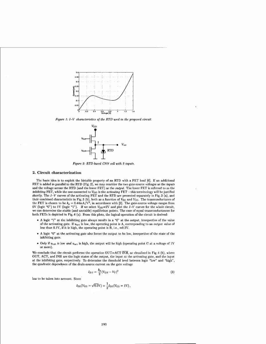
0-35 ; ■■ ./

0.3 ■ i / -

0.25 J 0.2

0.15

0.1

0.05

Vortag« [V]

Figure 1:I—V characteristics of the RTD used in the proposed circuit.

Figure 2: RTD-based CNN cell with 2 inputs.

2. Circuit characterization

The basic idea is to exploit the bistable property of an RTD with a FET load [6]. If an additional FET is added in parallel to the RTD (Fig. 2), we may consider the two gate-source voltages as the inputs and the voltage across the RTD (and the lower FET) as the output. The lower FET is referred to as the inhibiting FET, while the one connected to VDD is the activating FET - this terminology will be justified shortly. The I—V curves of the activating FET and the RTD are presented separately in Fig. 3 (a), and their combined characteristic in Fig.3 (b), both as a function of Vbs and VGS- The transconductance of the FET is chosen to be kp — 0.44mA/V2, in accordance with [2]. The gate-source voltage ranges from OV (logic "0") to IV (logic "1"). If we select VDD=2V and plot the I—V curves for the whole circuit, we can determine the stable (and unstable) equilibrium points. The case of equal transconductances for both FETs is depicted in Fig. 4 (a). From this plots, the logical operation of the circuit is derived:

• A logic "1" at the inhibiting gate always results in a "0" at the output, irrespective of the value of the activating gate. If uact is low, the operating point is A, corresponding to an output value of less than 0.1V, if it is high, the operating point is B, i.e., RS0.2V.

• A logic "0" at the activating gate also forces the output to be low, irrespective of the state of the inhibiting gate.

• Only if u;„h is low and u^-t is high, the output will be high (operating point C at a voltage of IV or more).

We conclude that the circuit performs the operation OUT=ACTINH, as visualized in Fig. 4 (b), where OUT, ACT, and INH are the logic states of the output, the input at the activating gate, and the input at the inhibiting gate, respectively. To determine the threshold level between logic "low" and "high", the quadratic dependence of the drain-source current on the gate voltage

IDS = ^(VOS-VT)2 (3)

has to be taken into account. Since

^DS(VGS : VÖI\) = i/DS(Vfcs = IV),

190

sil.O

0.2

5" E0.15 RTE> ■;'

/ : 1 '■/'■■ '

: Vj 3io.e

.io.e «0.1 S ' """t- *''

V

0.05

/ / /

* If/•*-■*' VJ is"0"4

-io.2 si0.0 V

0 IF?""" i _i 1 1 1

(a) RTD and FET separately

DS RTD l

(b) RTD and FET in parallel

Figure 3:1-V characteristic of an RTD and a FET with k^O.UmA/V*.

we get, for Vy = 0, a threshold voltage of 0.7V, which is indeed reasonable, as the NDR region in Fig. 4 (a) extends approximately from 0.4V to 1.0V - the threshold level lies exactly in the middle of these two boundaries. The circuit is extendible to multiple inputs in a straighforward manner by

Vinn

l.ov-

0.7V-

1 l_

A i B i _(low) _ l_(Io^)j_

I 1

(low)

S.lnh RTD '

(a) Combined I~V characteristics

Figure 4: Characteristics and output of the circuit as a function of Vact and V;„/,. VDD=^V.

0.7V 1.0V (b) Circuit output

including additional transistors parallel to the activating and inhibiting transistor, respectively.

3. Simulation results

In Fig. 5, the results of the Spice simulation are displayed. The two-dimensional plot (b) looks quali- tatively similar to Fig. 4 (b). Note the abrupt ascent of the voltage between the "low" and "high" output levels, the circuit produces a perfectly binary signal.

The size of the "high" (black) area increases with increasing transconductance of the transistors. To build a CNN cell, we basically need a comparator, i.e., an output function whose "high" area is a

triangle and ideally covers half of the input space. With 10 times larger transconductances, this can, in fact, be achieved closely, as depicted in Fig. 6. Due to the region of negative differential resistance, the

191

mm

(a) 3D plot (b) 2D plot with uniform grayscale

Figure 5: Circuit output as a function ofuact andu{„/, (Spice simulation).

(a) Decreasing u„t (b) Increasing uact

Figure 6. Comparator (Spice simulation). Hysteresis causes the slight difference between the two outputs.

transistion from the "low" to the "high" state (Fig. 6 (a)) does not occur at precisely the same voltage as the opposite transition (Fig. 6 (b)). This hysteresis may be overcome by using a clocked supply voltage, which would force the circuit to always start at the "low" state, as proposed in [7].

In the proposed circuit, the three basic ingredients needed for a fixed-template uncoupled CNN cell are implemented with a minimum amount of circuitry, by exploiting the physical properties of FETs and RTDs:

The input voltage is multiplied by the transconductance of the FETs.

The currents of the individual transistors, which are connected in parallel, sum up. The difference between the activating and the inhibiting current sum flows into the RTD. This is the task of the RTD. Depending on whether its current is negative or positive, it is put in one of the stable states, thus producing a binary output voltage.

This cell is, in fact, a circuit realization of the equation (1). In this context, the fixed template ß, is the so-called transconductance template. Since the relationship between the transconductance and the drain-source current is linear, existing template values can readily be used, as demonstrated in the next Section.

Multiplication:

Summation:

Nonlinear output function:

192

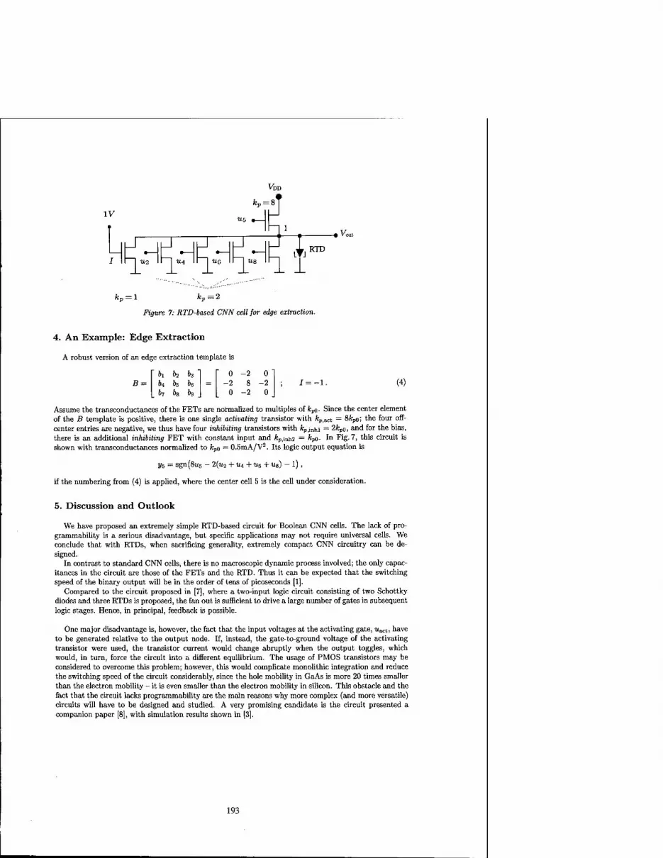
IV

«2 II I «4 II I «6 II I Us I it] RTD

Figure 7: RTD-based CNN cell for edge extraction.

4. An Example: Edge Extraction

A robust version of an edge extraction template is

&1 62 bs 0 -2 0 64 h be = -2 8 -2 67 6g 69 0 -2 0

J = -l. (4)

Assume the transconductances of the FETs are normalized to multiples of fcpo- Since the center element of the B template is positive, there is one single activating transistor with Ap,act = 8A;po; the four off- center entries are negative, we thus have four inhibiting transistors with kv;mhi = 2fcpo, and for the bias, there is an additional inhibiting FET with constant input and kPj\„h2 = fcpo- In Fig- 7, this circuit is shown with transconductances normalized to fc„o = 0.5mA/V2. Its logic output equation is

2/5 = sgn(8u5 - 2(«2 + Ui + ue+ it8) - l),

if the numbering from (4) is applied, where the center cell 5 is the cell under consideration.

5. Discussion and Outlook

We have proposed an extremely simple RTD-based circuit for Boolean CNN cells. The lack of pro- grammability is a serious disadvantage, but specific applications may not require universal cells. We conclude that with RTDs, when sacrificing generality, extremely compact CNN circuitry can be de- signed.

In contrast to standard CNN cells, there is no macroscopic dynamic process involved; the only capac- itances in the circuit are those of the FETs and the RTD. Thus it can be expected that the switching speed of the binary output will be in the order of tens of picoseconds [1].

Compared to the circuit proposed in [7], where a two-input logic circuit consisting of two Schottky diodes and three RTDs is proposed, the fan out is sufficient to drive a large number of gates in subsequent logic stages. Hence, in principal, feedback is possible.

One major disadvantage is, however, the fact that the input voltages at the activating gate, u&a, have to be generated relative to the output node. If, instead, the gate-to-ground voltage of the activating transistor were used, the transistor current would change abruptly when the output toggles, which would, in turn, force the circuit into a different equilibrium. The usage of PMOS transistors may be considered to overcome this problem; however, this would complicate monolithic integration and reduce the switching speed of the circuit considerably, since the hole mobility in GaAs is more 20 times smaller than the electron mobility - it is even smaller than the electron mobility in silicon. This obstacle and the fact that the circuit lacks programmability are the main reasons why more complex (and more versatile) circuits will have to be designed and studied. A very promising candidate is the circuit presented a companion paper [8], with simulation results shown in [3].

193

Acknowledgment

This work was partly supported by the ONR grant N00014-99-1-0339 and by the MUM ONR grant N00014-98-1-0594. We would like to thank Dr. D. H. Chow and Dr. J. N. Schulman for helpful discussions during the initial phase of this work.

References

[1] H. Mizuta and T. Tanoue, The Physics and Applications of Resonant Tunnelling Diodes. Cambridge University Press, 1995. ISBN 0-521-43218-9.

[2] K. J. Chen, T. Akeyoshi, and K. Maezawa, "Monolithic Integration of Resonant Tunneling Diodes and FETs for Monostable-Bistable Transition Logic Elements (MOBILEs)," IEEE Electronic Device Letters, vol. 16, pp. 70-73, Feb. 1995.

[3] M. Hänggi, R. Dogaru, and L. 0. Chua, "Physical Modeling of RTD-Based CNN Cells," in IEEE International Workshop on Cellular Neural Networks and their Applications, May 2000.

[4] J. N. Schulman, H. J. D. L, Santos, and D. H. Chow, "Physics-Based RTD Current-Voltage Equa- tion," IEEE Electronic Device Letters, vol. 17, pp. 220-222, May 1996.

[5] M. Bhattacharya and P. Mazumder, "SPICE Simulation of Circuits Containing Resonant Tunneling Diodes," in European Conference on Circuit Theory and Design, vol. 2, pp. 663-666, Aug. 1999.

[6] P. Mazumder, S. Kulkarni, M. Bhattacharya, J. P. Sun, and G. I. Haddad, "Digital Circuit Applica- tions of Resonant Tunneling Devices," Proceedings of the IEEE, vol. 86, pp. 664-686, Apr. 1998.

[7] D. H. Chow, H. L. Dunlop, S. E. W. Williamson III, B. K. Gilbert, S. Subramaniam, P.-M. Lei, and G. H. Bernstein, "InAs/AlSb/GaSb Resonant Interband Tunneling Diodes and Au-on-InAs/AlSb- Supperlatic Schottky Diodes for Logic Circuits," IEEE Electronic Device Letters, vol. 17, pp. 69-71, Feb. 1996.

[8] R. Dogaru, L. O. Chua, and M. Hänggi, "A Compact Universal Cellular Neural Network Cell Based on Resonant Tunneling Diodes: Circuit Design, Model, and Functional Capabilites," in IEEE Inter- national Workshop on Cellular Neural Networks and their Applications, May 2000.

194

2000 6™ IEEE International Workshop on Cellular Neural Networks and Their Applications Proceedings

The Design of Neuron-Bipolar Junction Transistor (vBJT) Cellular Neural Network(CNN) Structure with Multi-

Neighborhood-Layer Templates*

Wen-Cheng Yen and Chung-Yu Wu

Institute of Electronics and Department of Electronics Engineering National Chiao-Tung University Engineering Building 4th, 1001 Ta Hsueh Road Hsinchu, Taiwan, R.O.C. TEL: 886-3-5712121ext.54148 FAX: 886-3-5715412

E-mail: cywu@alab.ee.nctu.edu.tw &p8411827@alab.ee.nctu.edu.tw

ABSTRACTS compact and efficient neuron-bipolar junction Iransistor(vBJT) cellular neural network(CNN) structure with multi-neighborhood-layer templates is proposed and analyzed. Using the proposed structure, the coefficients of the templates with two neighborhood layers are fully realizable. But those with more than two neighborhood layers are constrained. As the demonstrative examples on the applications of the proposed vBJT CNNs, the functions of both de-blurring and muller-lyer arrowhead illusion functions have been successfully realized and verified by HSPICE simulation.

1. Introduction Since the invention of the cellular neural network (CNN) by Chua and Yang[l], many VLSI implementations

of CNNs have been proposed. Among them, the current-mode technique is used to implement CNNs with fixed weights[2]. The CNN with programmable weights is also realized in CMOS[3], Some effort is also devoted to implement CNNs using the basic physical characteristics of semiconductor devices[4]-[7]. Thus, the resultant CNN structures can be very simple and large-size CNNs can be integrated on a single chip. The proposed basic device structure to realize CNNs is called the neuron-bipolar junction transistor(vBJT)[4]-[8]. It has been applied to the implementation of compact CNNs with programmable symmetric templates and with a single neighborhood layer(r=l)[4] or multiple neighborhood layers(r>l)[5], the photo-input vBJT CNN[6], and the fully programmable CNNs with a single neighborhood layer (r=l) [7].

In some CNN applications like subcortical visual pathway[9] and de-blurring[10], the required templates are asymmetric with more than one neighborhood layers, i.e. r > 1. Although larger templates with r > 1 can be decomposed into smaller ones with r = 1[11]-[12] through some techniques expressed directly in terms of CNN structures, it is still very complicated to handle and generalize the proposed techniques for VLSI implementation of CNNs with r >1. So far, most VLSI implementation have been for CNNs with single neighborhood layer(r=l). The vBJT structure in [5] is used to realize CNNs with programmable templates of r>l. But only the symmetric templates can be realized. The vBJT structure in [7] can realize CNNs with templates of r>l but under some constraints on template coefficients. Thus both structures cannot implement the general templates of r>l in [5],

[7]. In this paper, the structure of fully programmable vBJT CNN[7] with a single neighborhood layers (r=l) is

modified to realize vBJT CNN with adjustable multiple neighborhood layers(r>l). The template coefficients of the r=2 neighborhood layer is a fully programmable but the r>3 neighborhood layer is constraint in a special template weight. The resultant structure is compact without adding too many extra devices. As the demonstrative examples on the applications of the proposed vBJT CNNs, the functions of both de-blurring and muller-lyer arrowhead illusion functions have been successfully realized and verified by HSPICE simulation.

2. Circuit Structure The proposed vBJT CNN general structure with adjustable multiple neighborhood layers is shown in Fig. 1

where the programmable weights of A and B templates are realized by a fully programmable stage PW containing two gate-controlled lateral PNP bipolar junction transistors (BJTs)QB2 and QB3 [13]-[16] and two MOS transistors MN6 and MP7. The cross-sectional view and the symbol of the gate-controlled lateral PNP BJTs are shown in Figs. 2(a) and 2(b), respectively. The current gain ß versus the collector current ICL for different gate voltages VGL from 4V to 3.4V is shown in Fig. 2(c). As shown in Fig. 2(c), the adjustable range of ß as controlled by V0L is approximately from 200 to 500 for ICL in the uA range. The absolute value of the weight can be changed by adjusting the gate voltage V0N of the coupling MOS resistor MN5 and the current gain ß of the lateral bipolar QB2 and QB3. To realize the sign of weights, the control voltages VSEL(-) and VSEL(+) are used to turn on MP7 for negative weights or MN6 for positive weights. The fully programmable stage PW is used to

' This work was supported by the National Science Council, R. O. C, under the contract NSC89-2215-E-009-051.

0-7803-6344-2/00/$10.00 ©2000 IEEE 195

realize the blocks PWA, PWA„ PWB, PWM> and PWBI. The degenerate stage PW with positive sign is used to realize the blocks PWA2 and PWB, as shown in Fig. 1.

M vc T

V<. 1 Vt[. 1

r-*ÄSr£«i /'' °TSM.)

-pt "Vj"-t r^ 4 4JvJ.,, w

- - - - Projrimnnblf Wrighl

iff Fig. 1 The general BJT CNN structure with multiple neighborhood layers.

B C. G E

Fig. 2 (a) The cross-sectional view and (b) The device symbol of the gate-controlled lateral bipolar junction transistor (BJT); (c) The current gain ß versus the collector current ICL for different gate controlled voltage V0L.

The A template is realized by the blocks PWA, PWA„ and PWA2. The neuron output current is sent to the neighboring neurons through the block PWA2 which performs the current to current conversion with a suitable positive gain. The template coefficients WATrof the rth neighborhood layer can be expressed as

WATr= WAIWA!W/ r=l,2 (!) where WA, WA1, and WA2 are the corresponding programmable template weights of the block PWA, PWAI, and PWA2, respectively. Given WATI and WAT2, WA and W^W« can be determined as

2 WAT WAT

WAT (2) WA = , WA<WAI

WAT,

According to (2), any template weights of WAT, and WAT2 can be designed by adjusting the programmable weights WA and WA, WA2.

In the cases of r>2, WA1> can be expressed as WAT, = Wm'-'l W„r2 = WAT1W;- r>2 (3)

1%

According to (3), the realizable multi-neighborhood-layer template for CNNs with 4 nearest neighborhood cells is shown in Fig. 3 where the master cell is shaded. In the layer of r=2, the template values of the cells receiving two flow paths from the shaded master cell are two-time larger than those receiving one flow path. The signs of WAT, for r>2 are constrained as listed in Table I.

Fig. 3 The realizable multi-neighborhood-layer A template for CNNs with 4 nearest neighborhood cells.

Table I The Sign Constraint of the Template Weights in the vBJT CNN with Multiple Neighborhood Layers.

WT, wT2 WATr(oddr) WATr(even r) Condition 1 + + + + Condition2 + - + - Condition3 - + - + Condition4 - - - -

Similar to the A template, the B template can be realized by the blocks PWB, PW„, PWB1, and PWB2. The input voltage Vm can be sent to other neighboring cells through the block PWB1 and the programmable weight blocks PWB and PWB2. Similar to (2), the weights W„, WB0, WB1, and WB2 of the blocks PWB, PWB0, PWBI and PWB2> respectively, can be expressed in terms of the given weights WBT0, WBT,, and WBT2 of the B template as

WBTI WBU1

WB = , WB,WB2 = , W„WBI + WK = IV,T« (4) W.n WBTI

Thus WB0 can be rewritten as

Wn = W™ — WBU

WB, (5)

From (4) and (5), the B template with two neighborhood layers can be realized by WB, WB0, WBI, and WB2. In the cases of more than two neighborhood layers, similar constraints on weight values and signs exit as in the A template.

3. Simulation Results To verify the correct functions of the proposed BJT CNN structure with multi-neighborhood-layer templates,

two examples are realized and simulated in HSPICE. The first example is the CNN for the de-blurring function. Both A and B cloning templates are given the Table II[10] where the B template has a single coefficient of WBT0. As compared with the A template structure in Fig. 3, the A template in Table II has four neighborhood layers with negative weights of WAT1= -0.6, WAT2= -0.3 or -0.5, WAT3= -0.2 or 0, and WAT4= -0.05 or 0. To realize the de-blurring function, the general structure of Fig. 1 can be reduced to that of Fig. 4. From (2) and table II, WA

and WJIWJU can be determined as WA=0.5 and WAIWA2= -1.2. From (4), WB0 can be determined as WB0=10. To minimize the errors in the weights of both third and fourth neighborhood layers, WA=l/3 and WA1WA2= —1.8 are chosen. To realize WA=l/3, WA1= -1.8, and WA2=1. The gate voltages VGN in the blocks PWA, PWA1, and PW„ are 1.82V, 3V, and 2.31V, respectively. The HSPICE simulated A template of the de-blurring vBJT CNN is shown in Fig. 5.

197

Table II The Templates of De-blurring CNN and

Muller-Lyer Arrowhead Illusion CNN

Application A B z De-blurring CNN

-0.05 -0.2 -0.3 -0.2 -0.05

-0.2 -0.5 -0.6 -0.5 -0.2

-0.3 -0.6 0 -0.6 -0.3

-0.2 -0.5 -0.6 -0.5 -0.2

-0.05 -0.2 -0.3 -0.2 -0.05

0 0 0 0 0

0 0 0 0 0

0 0 10 0 0

0 0 0 0 0

0 0 0 0 0

0

Muller-Lyer arrowhead illusion CNN

0 0 0 0 0

0 0 0 0 0

0 0 1.3 0 0

0 0 0 0 0

0 0 0 0 0

-0.1 -0.1 -0.1 -0.1 -01

-0.1 -0.1 -0.1 -0.1 -0.1

-0.1 -0.1 1.3 -0.1 -0.1

-0.1 -0.1 -0.1 -0.1 -0.1

-0.1 -0.1 -0.1 -0.1 -0.1

-2.8

Fig. 4 The reduced structure of Fig. 1 to realize the de-blurring vBJT CNN.

Fig. 5 The HSPICE simulated A template of the de-blurring vBJT CNN.

Fig. 6(a) shows the input image used to test the realized fully programmable vBJT CNN for the de-blurring function. The image size is 32x32 pixels. The HSPICE simulated output image from the de-blurring vBJT CNN is shown in Fig 6(b). It can be seen from Fig. 6(b) that the blurring effects of an optical device to give a sharply focused output image has been compensated. For the output gray-level image in Fig. 6(b), about 5% level shift is observed as compared to the input image.

(a) (b) Fig. 6 (a) The input image and (b) the final HSPICE simulated output image in the de-blurring vBJT CNN.

198

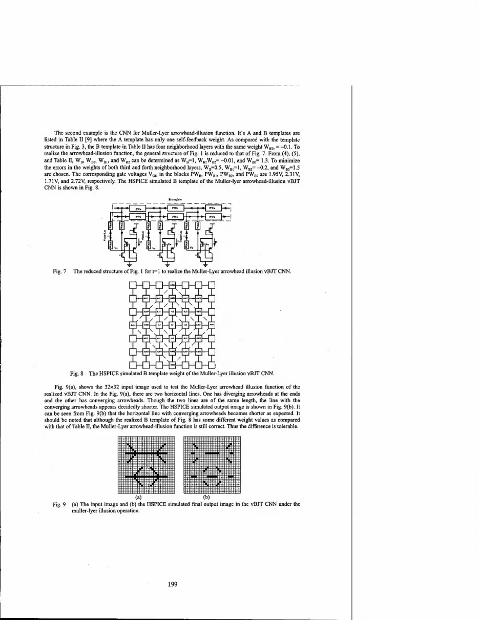
The second example is the CNN for Muller-Lyer arrowhead-illusion function. It's A and B templates are listed in Table II [9] where the A template has only one self-feedback weight. As compared with the template structure in Fig. 3, theB template in Table II has four neighborhood layers with the same weight WBTr =-0.1. To realize the arrowhead-illusion function, the general structure of Fig. 1 is reduced to that of Fig. 7. From (4), (5), and Table II, WB, WB0, WB1, and WB2 can be determined as WB=1, WB,WB2= -0.01, and WM= 1.3. To minimize the errors in the weights of both third and forth neighborhood layers, WB=0.5, WB,=1, WB2= -0.2, and WB0=1.5 are chosen. The corresponding gate voltages VGN in the blocks PWB, PWBI, PWB2, and PWB0 are 1.95V, 2.31V, 1.71V, and 2.72V, respectively. The HSPICE simulated B template of the Muller-lyer arrowhead-illusion vBJT CNN is shown in Fig. 8.

j Fffi \- -• \-*~\ PW» f* 1

Fig. 7 The reduced structure of Fig. 1 for r=l to realize the Muller-Lyer arrowhead illusion vBJT CNN.

Fig. 8 The HSPICE simulated B template weight of the Muller-Lyer illusion vBJT CNN.

Fig. 9(a), shows the 32x32 input image used to test the Muller-Lyer arrowhead illusion function of the realized vBJT CNN. In the Fig. 9(a), there are two horizontal lines. One has diverging arrowheads at the ends and the other has converging arrowheads. Though the two lines are of the same length, the line with the converging arrowheads appears decidedly shorter. The HSPICE simulated output image is shown in Fig. 9(b). It can be seen from Fig. 9(b) that the horizontal line with converging arrowheads becomes shorter as expected. It should be noted that although the realized B template of Fig. 8 has some different weight values as compared with that of Table II, the Muller-Lyer arrowhead-illusion function is still correct. Thus the difference is tolerable.

(a) (b) Fig. 9 (a) The input image and (b) the HSPICE simulated final output image in the vBJT CNN under the

muller-lyer illusion operation.

199

4. Conclusions A compact and efficient vBJT CNN with multi-neighborhood-layer template is proposed and analyzed. The

coefficients of the templates with two neighborhood layers are fully realizable. But those with more than two neighborhood layers are constrained in both sign and magnitude. Both de-blurring and Mullcr-Lyer illusion functions have been successfully verified in the programmable vBJT CNN by HSPICE simulation. Further applications of the proposed vBJT CNN will be explored in the near future.

5. Reference

[I] L. O. Chua and L. Yang, "Cellular neural networks: Theory and Applications," IEEE Tran. Circuit Syst., vol. 35, no. 10, pp.1147-1180 Oct. 1988.

[2] S. Espcjo, A. Rodriguez-VazqueZ, R. Domingucz-Castro, J L. Huertas, and E. Sänchez-Sinencio, "Smart- pixel cellular neural networks in analog current-mode CMOS technology," IEEEJ. Solid-Stale Circuits, vol. 28, pp. 895-905, Aug. 1994.

[3] P. Kinget and J. Steyaert, "A programmable analog cellular neural network CMOS chip for high speed," IEEEJ. Solid-State Circuits, vol. 30, pp. 235-243, Mar. 1995.

[4] W. C. Yen and C. Y. Wu, "A new compact neuron-bipolar cellular neural network structure with adjustable neighborhood layers and high integration level," in Proc. of IEEE International Symp. on Circuits and Systems, vol. 4, pp. 505-508, Jun. 1999.

[5] C. Y. Wu and W. C. Yen, "A new compact neuron-bipolar junction transistor (vBJT) cellular neural network(CNN) structure with programmable multi-neighborhood-layer symmetric templates for image processing, " submitted to IEEE Transactions on Circuits and Systems I: Fundamental Theory and Applications.

[6] C. Y. Wu and W. C. Yen, "An efficient and compact integration of CMOS image sensors and cellular neural network(CNN) for intelligent processing, " in Proc. of IEEE International Conference on Multisensor Fusion and Integration for Intelligent Systems, pp. 232-236, Aug. 1999.

[7] W. C. Yen and C. Y Wu, "A new compact programmable vBJT cellular neural network structure with adjustable neighborhood layers for image processing," in Proc. of International Conference on Electronics, Circuits and Systems, vol. 2, pp. 713-716, Sep. 1999.

[8] C. Y. Wu and W. C. Yen, "The neuron-bipolar junction transistor (vBJT)-a new device structure for VLSI neural network implementation," in Proc. of International Conference on Electronics, Circuits and Systems, vol. 3, pp. 277-270, Sep. 1998.

[9] T. Roska, J. Hämori, E. Labos, K. Lotz, L. Orzo, J. Takacs, P. L. Venetianer, Z. Vidnyansky, and A. Zarandy, "The use of CNN model in the subcortical visual pathway," IEEE Trans. Circuits Syst.-I, vol. 40, pp. 1822- 195, Mar. 1993.

[10] L. O. Chua, CNN: A paradigm for complexity, world scientific series on nonlinear science, vol. 31, no, 1998

[II] R. Akbari-Dilmaghani, "Mixed logic &ana!og implement of large neighborhood cloning templates for CNNs," in Proc. of the fith IEEE International Workshop on cellular networks and their applications, pp.277-281 Apr. 1998.

[12] M. H. ter Brugge, J. H. Stevens, J.A.G. Nijhuis, L. Spaanenburg, "Efficient DTCNN implementations for large-neighborhood functions," in Proc. of the fith IEEE International Workshop on cellular networks and their applications, pp.88-93 Apr. 1998.

[13] T. W. Pan and A. A. Abidi, "A 50-dB variable gain amplifier using parasitic bipolar transistors in CMOS," IEEEJ. Solid-State Circuits, vol. 24, pp. 951-961, Aug. 1989.

[14] S. Verdonckt-Vandebroek, S. S. Womg, C. S. Woo, and P. K. Ko, "High-gain lateral bipolar action in a MOSFET structure," IEEE Trans. Electron Devices, vol. 38, pp. 2487-2496, Nov. 1991.

[15] C. Laber, "Design considerations for a high performance 3 um CMOS analog standard cell library," IEEE J. Solid-State Circuits, vol. 22, pp. 181-189, Apr. 1987.

[16] M. G. R. DeGrauwe, O. N. Leuthold, E. A. Vittoz, H. J. Oguey, and A. Descombes, "CMOS voltage references using lateral bipolar transistors, "IEEE J. Solid-State Circuits, vol. 20, pp. 1151-1157, Dec. 1985.

200

2000 6™ IEEE International Workshop on Cellular Neural Networks and Their Applications Proceedings

The CNNUC3: An Analog I/O 64 x 64 CNN Universal Machine Chip Proto- type with 7-bit Analog Accuracy

G. IM&n, S. Espejo, R. Domlnguez-Castm and A. Rodriguez-Vdzquez

Institute de Microelectrönica de Sevilla - CNM-CSIC Edificio CICA-CNM, OTarfia s/n, 41012- Sevilla, SPAIN

Phone: +34 95 4239923, Fax: +34 95 4231832, E-mail: linan@imse.cnm.es

ABSTRACT This paper describes a full-custom mixed-signal chip which embeds distributed optical signal

acquisition, digitally-programmable analog parallel processing, and distributed image memory - cache - on a common silicon substrate. This chip, designed in a 0.5nm CMOS standard technology contains around 1,000,000 transistors, 80% of which operate in analog mode; it is hence one the most complex mixed-signal chip reported to now. Chip functional features are in accordance to the CNN Universal Machine [1] paradigm: cellular, spatial-invariant array architecture; programmable local interactions among cells; randomly-selectable memory of instructions (elementary instructions are defined by specific values of the cell local interactions); random storage/retrieval of intermediate images; capability to complete algorithmic image processing tasks controlled by the user-selected stored instructions and interacting with the cache memory, etc. Thus, as illustrated in this paper, the chip is capable to complete complex spatio-temporal image processing tasks within short computa- tion time ( - 200ns for linear convolutions) and using a low power budget (<1.2W for the complete chip). The internal circuitry of the chip has been designed to operate in robust manner with >7-bit equivalent accuracy in the internal analog operations, which has been confirmed by experimental. measurements. Hence, to all practical purposes, processing tasks completed by the chip have the same accuracy than those completed by digital processors preceded by 7-bit digital-to-analog con- verters for image digitalization. Such 7-bit accuracy is enough for most image processing applica- tions. CNNUC3 has been demonstrated capable to implement - either directly or through template decomposition - 100% of the linear 3x3 templates in reported [2].

1. Introduction'

Full exploitation of Cellular Neural Network capabilities for image processing can only be exploited through VLSI chips. Several CNN and CNN-UM chips have been made in the past; particularly, those having a size larger than 10 x 10 and whose operation have been actually demonstrated through experimental evidence are described in [3]-[6]. The chips in [3], [4] and [5] are intended for binary images, while that in [6] is intended for gray-scale images. Those in [4] and [5] have been designed by keeping analog accuracy and robustness as targets, while those in [3] and [6] are targeted for maximum cell density. Finally, only the chip in [5] embeds distributed optical sensors for direct optical image acquisition.

CNNUC3 also embeds distributed optical sensors - it is a true focal-plane analog programmable array processor - and is capable to acquire gray-scale inputs and produce gray-scale outputs. It has been designed to achieve around 7-bit equivalent resolution in the internal analog operations, and its robust operation has been experimentally dem-

onstrated through implementation of 100% of the linear 3x3 templates in reported [2], Besides, it can be directly interfaced to digital equipments and incorporate all functional features needed for the realization of complex image processing algorithms.

2. General Characteristics

CNNUC3 consists basically of an array of 64 x 64 identical cells. Its processing is continuous-time and spa- tially-invariant, with radius-1 neighbourhood and the cell state equation given by the FSR model [7].

Feedback and control templates, and the offset (or bias) term are programmable with a resolution of eight bits

t This work has been partially funded by ONR-NICOP N68171-98-C-90O4, DICTAMIST-1999-19007 and TtC 990826.

0-7803-6344-2/00/$10.00 ©2000 IEEE 201

Table 1: Prototype Data.

- seven + sign. Input and output pixel values are analog (gray-scale) in general. However, specific functions are included for binary (black&white) images, which can also be processed. Spatially-distributed image memories are available for storage of both analog and binary images on a pixel-by-pixel basis. This allows fully-parallel (64 x 64 wide) data-transference between processors and memory.

The prototype incorporates global-control and program- ming circuitry, located at the periphery of the array. This includes memory for 32 arbitrary sets of coefficients which, after programmed, can be randomly selected from the outside.

External control is completely digital. The interface has . been designed to be easily embedded in conventional digital

systems centred around a CPU or a DSP unit. Two bidirec- tional data-buses, one analog and one digital, are employed for image loading and downloading.

The prototype has been designed and manufactured in a 0.5um, single poly, three metal layer CMOS technology. Cell size is 102.2 x I20u.m2 - necessary to guarantee 7-bit equiva- lent accuracy in the internal analog operations, while total die size is 9.145 x 9.534mm2. The cell array occupies 58% of the die area. Nominal power supply is 3.3V, and worst-case power consumption is 1.2W. Table 1 shows the most relevant physical and electrical data of the prototype.

3. Chip Description

Fig.2 (a) shows the chip architecture. The prototype incor- porates some global-control and programming circuitry located at the array periphery. This includes memory for 32

arbitrary sets of CNN coefficients and for 64 arbitrary sets of

48 digital signals that are used as digital instructions to con- figure properly the cell in order to perform the different tasks that the cell is designed for. These memories can be randomly addressed from the outside once they have been programmed. Fig. 1 (b) shows the chip microphotograph.

# of Cells 4096(64x64 Array)

# of Transistors -1.000.000

# Transistors on the cell 172

Cell Size 120 (Am x 102.2 ^m

Cell Density ~82cells/mm2

Signal Swing [0.6, 1.4]V (Program- mable.)

Weight Swing [2.15, 2.95]V (Program- mable.)

Time Constant -1.2ns

Time Constant for Linear Convolutions

-200ns

Spatial Uniformity on the Weight Signals.

7.6-bits

I/O Digital Rate 10MHz

I/O Analog Rate 1MHz

Power Supply 3.3V

Power per cell 250|aW

Power Consumption 1.2W (worst case)

# of Templates Memo- rized

32

# of Instructions 64

Die Size 9145.10 nmx 9534 (im

rt

P

^

Analog I/O,Data bus

CELL ARRAY on

PROGRAMM. CIRCUITRY

Digital I/O Data bus

Fig. 1: (a) Chip Architecture.

9.145mm

Fig. I: (b) Chip Micmphotograpky

202

DI Bus AR Bus

rr AW£BCBus

rr

DI: Digital Instruction AI: Analog Instruction MB: Memory Block

4 6:64 Dec.

DI KAM 54x3 bytes

|DACS(8) 1 DACs(22) |

AR RAM 32x8 bytes

AW&BCRAM L 32x22bytes |

St 3JT

WH -M

AW: Analog Weights BC: Boundary Conditions AR: Analog References

Digital Data bus

Fig; 2: Program storage and global control circuitry: functional description.

3.1 Programming Circuitry

3.1.1 Program-Memory Structure

Fig.2 shows the peripheral programming blocks, including three parts. The first two parts are devoted to storage of 32 analog

coefficient sets; 32 "analog instructions" can hence be stored on chip - one per coefficient set. Coefficients included into each set are classified in two groups. The first contains CNN processing parameters (9 feedback

template elements, 9 control template ele-

ments, 2 bias terms, and 2 boundary condi-

tion levels). The second contains 8 analog reference levels that control electrical opera- tion of the network (maximum, zero, and minimum values of the weight- and the state-variable signals, plus two additional analog biasing levels). Thus, a total of 30 analog coefficients are included at each of the 32 sets. Coef-

ficient values are defined by 8 -bits word, using a 7 bits+sign criterion, and are grouped into 16 -bits words to match the width of the external digital data bus. Digital data stored at the RAM are used to drive digital to analog (DA) converters to obtain 30 analog programming levels, which are transmitted to the cell array trough global routing lines.The third part of the programming circuitry is dedicated to the storage of digital control words. The number of internal digital control signals required to perform the different operations is 35. In order to have sufficient flex- ibility for chip operation while at the same time having a simple external interface, values of digital control signals are grouped in vectors (digital/control instructions) of 48 ( 3 x 16 ) bits, which must be previously written (pro-

grammed) in a 64 words RAM. Afterwards, these vectors can be selected (and therefore applied to the network) using a small address bus.

3.2 CNN Circuitry

3.2.1 Synapse

Every cell in the array contains 20 synapses: 9 for he feedback template, 9 for the control template, and 2 for

the offset term. Each synapse is driven by an input signal (either vcx, vc

u, or vlal) and by a global weight-program-

0,1,..., 9 ), both of them in voltage form. Input signals vcx and i\ are local to

cell and taken from the corresponding capacitors Cx and C„, while the weight signals (and also the saturation level

vJ0,) are global (common to all cells in the array), as required for a spatially uniform CNN. The weight signals and

the saturation level (and some other 9 analog voltages) are generated by DA converters driven by the selected ana- log instruction in the programming circuitry. The output of the synapse is in current form. All current contributions to each cell are added at the cell' input node.

The synapse circuit is based on a circuit technique [8] that provides a four-quadrants-synapse behaviour from a single MOS transistor operating in its ohmic region, at the expense of a previous calibration step. The calibration step is needed because the synapse output current contains an "offset term". In particular, each synapse output, is of the form

ming signal (vj or vdB , with d

's = ',(yfvw>=GK)vi+1oK) (1)

where v, is some vx, vu, or vja,, and vn some vA or vB . Both v, and vn are relative to their corresponding

203

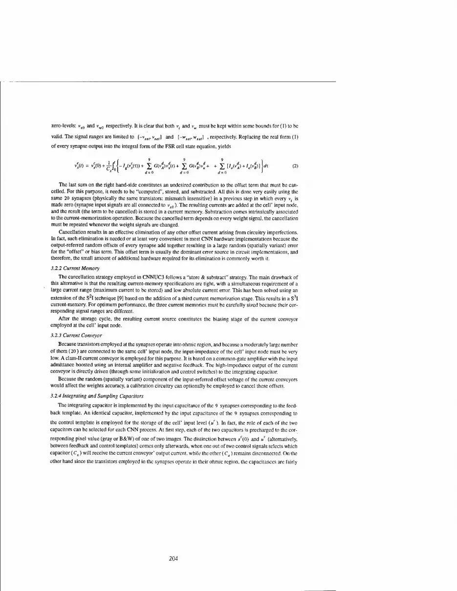
zero-levels: v^,, and vw0 respectively. It is clear that both vt and vn. must be kept within some bounds for (1) to be

valid. The signal ranges are limited to l-vtar vlal] and [-wJor wlal] , respectively. Replacing the real form (1)

of every synapse output into the integral form of the FSR cell state equation, yields

C 9 9 9 •, "»(') = »*«>) + £" U - V^(x)) + £ G(vd

A)/x(,) + X G(vJ)vf + + £ [/„(vj) + /„($] U (2) * I d = o d = o <; = o J

The last sum on the right hand-side constitutes an undesired contribution to the offset term that must be can- celled. For this purpose, it needs to be "computed", stored, and substracted. All this is done very easily using the same 20 synapses (physically the same transistors: mismatch insensitive) in a previous step in which every v- is made zero (synapse input signals are all connected to vx0). The resulting currents are added at the cell' input node, and the result (the term to be cancelled) is stored in a current memory. Substraction comes intrinsically associated to the current-memorization operation. Because the cancelled term depends on every weight signal, the cancellation must be repeated whenever the weight signals are changed.

Cancellation results in an effective elimination of any other offset current arising from circuitry imperfections. In fact, such elimination is needed or at least very convenient in most CNN hardware implementations because the output-referred random offsets of every synapse add together resulting in a large random (spatially variant) error for the "offset" or bias term. This offset term is usually the dominant error source in circuit implementations, and therefore, the small amount of additional hardware required for its elimination is commonly worth it.

3.2.2 Current Memory

The cancellation strategy employed in CNNUC3 follows a "store & substract" strategy. The main drawback of this alternative is that the resulting current-memory specifications are tight, with a simultaneous requirement of a large current range (maximum current to be stored) and low absolute current error. This has been solved using an

extension of the S2I technique [9] based on the addition of a third current memorization stage. This results in a S3I current-memory. For optimum performance, the three current memories must be carefully sized because their cor- responding signal ranges are different.

After the storage cycle, the resulting current source constitutes the biasing stage of the current conveyor employed at the cell' input node.

3.2.3 Current Conveyor

Because transistors employed at the synapses operate into ohmic region, and because a moderately large number of them (20) are connected to the same cell' input node, the input-impedance of the cell' input node must be very low. A class-II current conveyor is employed for this purpose. It is based on a common-gate amplifier with the input admittance boosted using an internal amplifier and negative feedback. The high-impedance output of the current conveyor is directly driven (through some initialization and control switches) to the integrating capacitor.

Because the random (spatially variant) component of the input-referred offset voltage of the current conveyors would affect the weights accuracy, a calibration circuitry can optionally be employed to cancel these offsets.

3.2.4 Integrating and Sampling Capacitors

The integrating capacitor is implemented by the input capacitance of the 9 synapses corresponding to the feed-

back template. An identical capacitor, implemented by the input capacitance of the 9 synapses corresponding to

the control template is employed for the storage of the cell' input level (u). In fact, the role of each of the two capacitors can be selected for each CNN process. At first step, each of the two capacitors is precharged to the cor-

responding pixel value (gray or B&W) of one of two images. The distinction between /(0) and u (alternatively, between feedback and control templates) comes only afterwards, when one out of two control signals selects which capacitor (Cx) will receive the current conveyor' output current, while the other (Cu) remains disconnected. On the

other hand since the transistors employed in the synapses operate in their ohmic region, the capacitances are fairly

204

linear.

3.2.5 Voltage Limiter

There are several very simple and hardware-efficient ways to implement the nonlinear resistor needed at the FSR cell state equation. A possibility is using two diodes and two reference levels. Diodes can be emulated using MOS transistors with moderately large aspect-ratio. This approach, however, has the disadvantages of smooth transition and finite slope in the saturation region and, much more important, its sensitivity to mismatch produces a random spatial variation of the cell saturation level. Note that the contribution of one cell to their neighbours, which is always proportional to the corresponding weight, is also proportional to the local value of vja, whenever the cell is saturated. Cell saturation occurs in many propagative templates, at the final steady state in binary output applica- tions, and at the beginning of the transient in binary input applications. In other words: in practically all CNN processing functions. Therefore, the accuracy and uniformity of the local saturation levels is as important as the accuracy and uniformity of the weights.

Another alternative is based on using active diodes, which employ negative feedback to achieve abrupt transi- tion, closer to the ideal, but still sensitive to mismatch due to amplifier offsets. A previous offset calibration cycle could be used to eliminate this effect, at the expense of a more complex circuitry and some additional global control lines. Still, one problem would be present: a substantial amount of power is needed in order to obtain sufficiently fast "diodes" without a significant overshoot (i.e., with a dominant time constant well below that of the CNN processing circuitry).

For these reasons, the limiter circuitry employed in CNNUC3 is somewhat involved. It is based on two compa- rators that detect when the cell' signal goes beyond either border of the linear region. In that case, the integrating capacitor is directly connected to one of two global wires driven by the corresponding saturation level -vsal or vsat,

whichever corresponds to the reached border. Although the input-referred offsets of the comparators will result in small errors, this deviations are effective only during the small transient (response time) of the comparator. Some minor additional tricks are needed to avoid possible instabilities in the proximity of the border points, and to allow for the state-variable signal to re-enter the linear region.

3.2.6 Initialization and Control Circuitry

A number of analog switches in every cell, and a similar number of global control lines are required to control the different cancellation circuits, the initialization process, and to actually launch the CNN transient. As a matter of fact, most of the control circuitry and global control lines are related to the enhanced functionalities described below.

33 Enhanced Functionalities

Additional functionalities have been incorporated for further improvement of the CNN Universal Machine capa- bilities [1] as required for relevant processing functions.

3:3.1 Image Memories

Every cell has the capability of storing four analog (gray-scale) and four binary (black & white) pixel values. At system level, this means that the chip can simultaneously store eight different images. These images can be used as inputs at any time during aprocessing sequence, and modified at any time as well; writting/reading time of the mem- ories is around 0.1 u.s. Binary memories employ conventional digital latches, while analog memories relay on "bot- tom-plate sampling" switched-capacitor stages following the guidelines given in [10]. By using these memories for storage of intermediate results significant computation time reductions are achieved in the realization of complex algorithms requiring iterative template applications, as well as in the realization of biffurcated-flow algorithms.

3.3.2 Local Logic Unit

The local logic unit (LLU) is a programmable boolean gate whose truth table is defined as part of the digital instructions stored in the programming circuitry. It allows a completely parallel realization of arbitrary bit-to-bit logic operations between images stored at two user-selectable binary memories. The resulting image can be down-loaded or stored in any of the four binary memories. Conventional digital circuitry is employed for this pur- pose.

205

3.3.3 Freezing Mask

Having a "freezing" mask means that the content of one user-selectable binary image memory can (optionally) be used as a flag which disables the evolution of the marked pixels during CNN processing transients, keeping their state variables time-invariant. The realization of this function requires just a few analog switches.

3.3.4 Global Gates

In many cases it is interesting to find out if some specific image is completely white or completely black, without wasting the time required to download the whole image. The prototype incorporates two global gates, one NAND and one NOR, to perform these logic operations over the pixel values of one user-selectable binary memory. With this functionality, the time required to check if some image is completely black or white is around 3ns.

3.3.5 Optical Input

In many real-life high-speed applications, the information to be processed by the network is an image that is available in optical form while the output contains only a few details extracted from the input. In these situations, the read-out process is extremely simplified and hence speeded up. However, the input image is always a complete frame and therefore, the time needed to transfer the image to the array can constitute an actual bottleneck. In those cases, the capability of combining the sensory and the processing planes, provides a dramatic system performances enhancement, since it produces systems that do not only exploit the advantages of the fully parallel processing but also those of the fully parallel image acquisition that are provided by a matrix of photosensors merged with that of processors. CNNUC3 incorporates a photosensing device within each cell that allows the acquisition of images that are directly projected over the silicon surface. The sensing scheme is based on the integration, in the capacitor of any of the analog image memory, of the current that is generated by a diffusion-substrate photodiode.

4. Conclusions

This paper describes a recently designed analog programmable array processor chip. The new prototype, called CNNUC3, contains 64 x 64 cells arranged onto an array and follows the CNNUM computing paradigm. For that purpose it includes several specially designed modules like the Local Logic Unit, the Local Analog Memory, the Switch Configuration Register, the Global Gates or the Freezing Map, that increase prototype capabilities. The chip is able to process, store and provide gray-scale images. An optical acquisition mode is also available thus allowing not only the full exploitation of the parallel processing but also of the parallel acquisition.

5. References

[1] T. RoskaandL.O. Chua, "The CNN Universal Machine: An Analogic Array Computer". IEEE Trans. Circuits and Systems II, Vol. 40, pp 163-173, March 1993.

[2] T.Roska, L. Kek, L. Nemes, Ä. Zarändy, M. Brendel, CSL ■ CNN Software Library ■ Version 7.2, Analogical and Neural Computing Laboratory, Computer and Automation Institute, Hungarian Academy of Sciences, Budapest, 1998.

[3] A. Paasio, V. Porra, "A CNN Universal Machine with 295 cells/mm2". Proc. of the 1997 Int. Symposium on Non Lineal Theory and its Applications (NOLTA'97), Honolulu, USA, 1997, pp. 221-224.

[4] P. Kinget and M. Steyaert, Analog VLSI Integration of Massive Parallel Processing Systems. Klüver Academic Publishers, ISBN: 0-7923-9823-8, 1997

[5] R. Domfnguez-Castro et al., "A 0.8u.m CMOS 2-D Programmable Mixed-Signal Focal-Plane Array Processor with On-Chip Binary Imaging and Instructions Storage". IEEEJ. Solid-Slate Circuits, Vol. 32, pp. 1013-1026, No. 7, July 1997.

[6] J. Cruz and L. Chua, "A 16X16 Cellular Neural Network Universal Chip". Analog Integrated Circuits and Signal Processing, Vol. 15, pp. 226-238, March 1998.

[7] S. Espejo, R. Carmona, R. Domfnguez-Castro and A. Rodriguez-Vazquez, "A VLSI-Oriented Continuous-Time CNN Model". International Journal of'Circuit Theory and Applications. Vol. 24, pp 341-356, May-June 1996.

[8] R. Dominguez-Castro, A. Rodriguez-Vazquez, S. Espejo, R. Carmona, "Four-Quadrant One-Transistor-Synapse for High-Density CNN Implementations". Proc. of 5th IEEE Int. Workshops on Cellular Neural Networks and their Applica- tions, pp. 243-248, London, April 1998.

[9] J.B. Hughes and K.W. Moulding, "S2I: A Two-Step Approach to Switched-Currents". Proc. 1993 IEEE Int. Symp. Circuits andSyslem, pp. 1235-1238, Mayl993.

[10] R. Carmona, S. Espejo, R. Dominguez-Castro, A. Rodriguez-Vazquez, T. Roska, T. Kozek, L.O. Chua, "A 0.5 (im CMOS CNN Analog Random Access Memory Chip for Massive Image Processing". Proc. of 5th IEEE Int. Workshops on Cellular Neural Networks and their Applications, pp. 271-276, London. April 1998.

206

2000 6™ IEEE International Workshop on Cellular Neural Networks and Their Applications Proceedings

A Programmable Vision Chip for CNN Based Algorithms

A. Dupret, J.O. Klein, A. Nshare

Institut d'Electronique Fondamentale, UMR 8622, Bätiment 220, Universite de Paris XI, 91405 Orsay cedex, France. (+33) 1 69 15 65 72, Antoine.Dupret@ief.u-psud.fr

Abstract: In this paper, an original architecture of CNN vision chip is adressed. In the introduction, an analyse of the limitations of the usual approaches leads us to propose an original architecture. The first part of the paper is dedicated to the description of the three main blocks of our vision chip. Then, the major building blocks are detailled Finally, design considerations and the pratical implementation of a typical CNN algorithm are discussed in the two last sections of this paper.

1. Introduction

Inspite of the increase of the computations capabilities resulting from the Moore's law, some complex tasks such as image processing at video rate are out of reach for many incomming generations of digital processors. So, many electronic architectures and algorithms were investigated to face this challenge. Considering the natural parallelism of the image, most of the architectures which have been explored, relies on the parallelisation of the computation.

The CNNs constitute a class of algorithms specially well suited for an implementation on massively parallel computers [1,2]. The concept of the electronic retina, which are a subset of CNNs [3], has been developped so as to take benefits from the natural parallelism of the image at the sensor level. Several vision chips have been designed, comprising photosensors and electronic operators for the execution of CNN algorithms [4-6].

When designing CNN vision chip, several constrains arise. In particular, each cell of the circuit must features a low power consumption and a high integration density in order to be compatible with an useful resolution of the image. Hence, most CNN chips reported, features analogue processings. Parametric operators have been designed so that various functions can be implemented, and consequently, varied kind of processing [4, 6, 7]. Such an approach is a sure improvement compared to the original concept of electronic retina.

Using analogue processing elements along with the high degree of parallelism lead to particularly short computation times. On the other hand, the analogue operators suffer some limitations such as the kind of functions which can be implemented. They also require great care of design. At the same time, the area of the pixels often remains too large regarding the resolutions required for an effective application [8].

Hence, in this paper we propose an original architecture allowing the implementation of CNN algorithms on an operational circuit. It is a question of reducing the degree of parallelism to increase the resolution. Besides, vre describe an analogue-digital structure of processors allowing to perform sequences of instructions such as Multiplications-Accumulations (MAC), comparisons or also boolean operations. In this paper, we shall begin by describing the architecture of circuit. Then, we shall present the different essential cells designed for our architecture. Finally, we shall depict the implementation of some algorithms by this circuit.

2. Architecture

2.1. Guideline

To reduce the area of the pixels to the minimum, while preserving a short time of image processing, we chose to concentrate the processing on a row of processors. Such approach presents the advantage to enable the design of complex processing units (so of important area) without lessening the resolution. In return, because the parallelism is reduced to a row, the computations which bring in more than one pixel henceforth have to be performed in a sequential way. However, if a sequential execution increases the time of processing for a given operation, it allows a more flexible process. Furthermore, it becomes possible to link up basic functions in an arbitrary order, as in any digital SIMD computer. The architecture is shown on Figure 1. We can discern the three main blocks we will now describe : an array of memory and photosensors, the row of processing elements, and the control block

0-7803-6344-2/00/$10.00 ©2000 IEEE 207

Array of Photosensors and analogue memory map.

row of processing units

Figure 1: Architecture

2.2. Array of photosensors and analogue memory map

The semi-parallel treatment that we chose imposes to store intermediary variables for every pixel. Since it must be possible to randomly access the photosensors, it was natural that every pixel includes several memories besides the sensor, as shown on Figure 1. To reconcile efficiency and compactness, a pixel is constituted of four capacitors acting as memories. The fourth memory element is also used to store the analogue voltage deriving from the sensor. The pixels of a same column exchange their data with the corresponding processing element through a Digital Analog Bus (DAB). So as to access any of its four memory elements, each pixel includes a bidirectionnal 4 to 1 multiplexer.

2.3. Column of processors

Derived from [ 1 ], the Figure 2 represents the diagram of a discret time CNN. From this figure and by resuming various works on the image processing, we identified some essential primitives.

*[B] nf(8K0 T f

.<&*

.[A]

Fig 2 : Discrete time CNN

First of all, the processing element must be able to make Multiplication-ACcumulations (MAC) to allow operations such as the linear spatial or temporal filtering of an image. Operations of comparison are also necessary to perform functions with thresholds. So as to enable conditional instructions or implementation of piece wise linear functions, a condition register is included in each processor. Finally, boolean operations were implanted. The boolean operators can be used to process the results of the comparisons and are useful during operations of mathematical morphology. The intermediate results can be stored in a local register and brought back in the processing element. To enable computations on data of pixels from different lines, a 3 to 1 multiplexer is inserted between the processors and the pixels.

2.4. Control

Pixels and processors require a complex control. But the optimal exploitation of the performances of such circuit within a system implies a simple interface. A microcontroller was so integrated into the circuit. The instruction set of the micro controller handles the analogue operations and is locally decoded. This approach allows to generate an arbitrary sequence of instructions and the design of the on-chip instruction decoder prevents conflicts between analogue signals.

208

ft DAB . riglh W

1 ♦ F \ MUX /

_[\ST_ analogu« eomparatcr AA ^ «neiogu* procetsing unit ^

1 ^--1 /x«

riiB^ —|_3£j—[3 <d 1 C^ 1 /x/vrcB|—<

_nj^ ' A A

_nj-i_ bocfcwi wit j-Ln_

local rtgiitef s J-LTL ' U>V L ng.,.n|n—[M"^< , J> H^

L-^ <j" Global Bus "~^>

Figure 3 : Mixt mode processing unit

3. The basic cells

3.1. Pixel

The array of pixels constitutes the core of our architecture. In this paragraph, we describe the photosensor as well as the memory elements of the pixel.

The photosensor is constituted by two minimum size vertical bipolar transistors. Associated in parallel, they form phototransistors. For a given surface, this disposal increases the sensitivity while preserving a large bandwidth [9]. The selected mode for the transduction of the light is the integration mode. The photosensor is then used as a current source which discharges a capacitor beforehand loaded to a voltage V,,/.

MOS capacitors are used as analogue or digital memories. The MOS capacitor associated to the photosensor is also considered as a memory. A set of switches makes possible to select the voltage stored in one of four capacitors. This voltage is copied out on the DAB thanks to a bi-directional amplifier. The same amplifier is used to write on one of four capacitors the voltage which is present on the DAB. To reach a clock frequency of 10 MHZ, the amplifier is designed so that a voltage copied out on the DAB reached its final value within 0.05 us.

3.2. Digital Analogue processors

As shown on Figure 3, the analogue-digital processor is constituted, on the one hand of logical gates for the non- linear operations, and on the other hand, for the linear computations, of an analogue processing unit. In this paper, we shall detail only the unity of analogue processing unit.

. Cin2 cin1 =pi ! jnra>--: ; ~~jL 1—•■'

Vdd 2

outPA >

Figure 4: Analogue Processing Unit

209

The Analogue Processing Unit (APU) derives from switched capacitors integrators [10, 11]. It contains three capacitors, one OTA and a set of switches controlled by the microcontroller. The Figure 4 details its functioning. The capacitor C„, is used as an accumulator. Thanks to the OTA, the charge stored in capacitor C,„, is transfered towards C„, so that it adds or subtracts. Furthermore when the capacitor CM is first shorted, and then put in parallel with CM, the charges balance among C,„, and CM. As a result, this sequence of operations achieves the division by two of the present charges on the two capacitors C,„, and CM. Hence, the transferred charges can be divided by two. The multiplication by a constant is then obtained in N instructions containing a succession of N divisions by two, where Nis the number of bits used to represent a fixed point coefficient. The datum is so multiplied by a coefficient

N

of the form Xa, '2~' ■ The possible problems of saturation are so avoided because the coefficient multiplier is i=l

always less than 1. The combination of divisions by two and of additions or of subtractions executes the MAC required in filtering. Besides, this structure, along with the other elements of the processing unit, allow to make the digital to analogue conversion of a data which would be then used by the APU. With the comparator, enclosed in the APU, it is also possible to use this structure as an analogue to digital converter.

Such structure combines the advantages of a versatile ALU and the density of integration of the analogue operators.

4. Design considerations

In order to validate our architecture, we designed an evaluation circuit including 16x16 pixels, 16 processing units and a control unit. The vision chip has been design in a 0.6 urn CMOS technology. At a first order, the accuracy of the computations depends on the distribution of the values of the components. So, when designing our vision chip, we chose that all the capacitors would have the same value. Hence a carefully drawn layout allows to reduce the spreading of the relative values of the components. In a 0.6 urn CMOS technology a cell processing unit occupies 50 X 200 pm2, that is 1/10000 of the surface of an integrated circuit of 1 cm2. This vision chip which been sent to foundry and its main characteristics are summarized in Table 1. The estimated characteristics of a 128 x 128 pixel operationnal chip are given in Table 2.

Total area of the circuit lOmra' Resolution (pixels) 16x 16 Number de processing unit 16 Area per Pixel 50 x 50 urn2

Area per par processing unit 50 x 200 urn2

Clock frequency lOMhz Pixel power consumption lOOnW Procesing Unit power consumption 300nW

Table. I : Main Characteristics of the Evaluation Circuit

Total area of the circuit 1cm' Resolution (pixel) 128x 128 Number de processing unit 128 Area per Pixel 50 x 50 u Area per par processing unit 50 x 200 u Area of the microcontroller 20mm Clock frequency lOMhz 128 MAC x 5 bits duration (5) 10 MHz Ills

Table. 2: Main Characteristics of the 128 X 128 pixel vision chip

5. Implementation of some typical CNN algorithms

We present in this paragraph the sequences of microcode allowing the implcmantation of some functions required in typical CNN algorithms. By resuming the figure 2 « principle of a discret time CNN », we identify 3 main functions to implement.

210

5.1. 3x3 Convolution

The 3x3 convolution product constitutes the base of the filtering in image processing. It is also in the body of theCNNs.

// 0 0.125 0 // 0.125 0.5 0.125 // 0 0.125 0 // 3-by-3 Kernel Conv :

Cin = i;' - ■■ - n

Cin *= Cin *= Cin Cout Cin =

u[i-l,j] 0.5 0.5 0.5 Cin

. = u[i,j-l] Cin *= 0.5 Cin *= 0.5 Cin *= 0.5 Cout += Cin ~J- - u[i,j]

= 0.5

Cout += Cin Cin = u[i,j+l] Cin *= 0.5 Cin *= 0.5 Cin *= 0.5 Cout += Cin Cin = u[i,j'+l] • .Cin *= 0.5 Cin *= 0.5 Cin *= 0.5 Cout += Cin next_x[i,j] = Cout

Cin = Cin

5.2. Temporal integration

Thanks to the register included in the processing unit, the temporal integration can be efficiently implemented.

// integrate Cin = integrated_x[i,j] Cout += Cin Cin = x[i,j] Cout += ein integrated_x[i,j] = Cout

5.3. Piecewise linear function

Piecewise linear function can be used to approximate any function. Here we present the code for the absolute value function.

// Absolute value : Cout = 0 Cin = Global_Ref(0) Cout += Cin Cin = x[i,j] if (Cout < Cin){

Cin = Cout Cout = 0 Cout -= Cin

} 5.4. Duration of a typical sequence

An evaluation of the required time to perform a CNN algorithm is given in table 3. It appears that a CNN algorithm can be performed in about 100 instructions and hence requires 1.28 ms for a 128x128 image. This makes it compatible with video rate processing.

211

Timing of CNN functions Functions Instructions Duration 2 x 3-by-3 Convolution 50 5 us Time integration 5 0.5 us Non-linear function (3 segments) 20 2 us Others (DC offset, loop control...) 25 2.5 us Total for one row 100 10 us Total for 128 rows 12,800 1.28 ms

Table. 3 : Main Characteristics of the Evaluation Circuit

6. Conclusion

We presented the original architecture allowing to acquire, then to process images by a succession of arbitrary operations. Although the processing times are longer than with the completely parallel architectures but stay under 20 ms for typical computations. Our approach allows to acquire images presenting an useful resolution while ensuring times of processing compatible with the video rate. Our architecture takes the advantage of the CNN algorithms while overcoming the limitations bound to surface consumming distributed operators in all the pixels.

7. Bibliography

[I] L. O. Chua and L. Yang, "Cellular Neural Networks: Theory," IEEE Transactions on Circuits and Systems,vo\. 35, pp. 1257-1272, 1988.

[2] L. O. Chua and L. Yang, "Cellular Neural Networks: Applications," IEEE Transactions on Circuits and Systems, vol. 35, pp. 1273-1290, 1988.

[3] L. O. Chua and B. E. Shi, "Resistive Grid Image Filtering: Input / Output Analysis Via the CNN Framework.," IEEE transactions on Circuits and Systems, vol. 39, pp. 531-548, 1992.

[4] A. Rodriguez-Vazquez, S. Espejo, R. Dominguez-Castro, R. Carmona, and E. Roca, "Mixed-Signal CNN Array Chips for Image Processing." SPIE, vol. 2950, pp. 218-229, 1996.

[5] S. Espejo, A. Rodriguez-Vazquez, R. Dominguez-Castro, and J. L. Huertas, "Smart-Pixel Cellular Neural Networks in Analog Current-Mode CMOS Technology.," IEEE Journal of Solid State Circuits, vol. 29, pp. 895- 904, 1994.

[6] P. Kinget and M. S. J. Steyaert, "A Programmable Analog Cellular Neural Network CMOS Chip for High Speed Image Processing," IEEE Journal of Solid-Stale Circuits, vol. 30, pp. 235-243, 1995.

[7] S. Espejo, R. Dominguez-Castro, A. Rodriguez-Vazquez, and R. Carmona, "Weigth-Control Strategy for Programmable CNN Chips," presented at CCNA-94 IEEE International Workshop on Cellular Neural Networks and their Applications, Rome Italy, 1994.

[8] K. Kyuma, E. Lange, J. ohta, A. Hermanns, B. Banish, and M. oita, "Artificial Retinas-Fast, Versatile Image Processors," Nature, vol. 372, 1994.

[9] A. Dupret, E. Belhaire, and J.-C. Rodier, "A high current large bandwidth photosensor on standard CMOS Process," presented at EuroOpto'96, AFPAEC, Berlin, 1996.

[10] C. Eichenberger and W. Guggenbuhl, "On Charge Injection in Analog MOS Switches and Dummy Switch Compensation Techniques.," IEEE Trans, on Circuits and Systems, vol. 37, pp. 256-264, 1990.

[II] D. J. Allstot and W. C. Black, "Technological Design Consideration for Monolithic MOS Switched- Capacitor Filtering Systems.," Proceedings of IEEE, vol. 71, pp. 967-986, 1983.

212

2000 6™ IEEE International Workshop on Cellular Neural Networks and Their Applications Proceedings

A STORED PROGRAM 2ND

ORDER/3-LAYER COMPLEX CELL CNN-UM

Cs. Rekeczky*, T. Serrano-Golarredona , T. Roska*, and A. Rodriguez-Vazquez'

""Analogical and Neural Computing Laboratory, Computer and Automation Institute, Hungarian Academy of Sciences, H-I 111 Budapest, Kende u. 13-17, Hungary

"instituto de Microelectronica de Sevilla, Centre de National de Microeletrönica, Ed. Cica, Avda. Reina Mercedes s/n. Sevilla 41012, Spain

ABSTRACT: A stored program 2nd order/3-layer complex cell Cellular Neural Network Universal Machine (CNN-UM) architecture is introduced. We discuss a number of phenomena that can be generated in this system by a single CNN transient. In particular, it is pointed out that by a proper combination of two dynamic layers some operations can be easily implemented that would require an approximation or iterative algorithmic solution relying on a first order CNN system. Thus, during these experiments, in a T order/3-layer CNN new multi-layer templates have been identified as efficient basic building blocks for various application motivated analogic algorithms.

Introduction

In recent years, design and theoretical analysis of CNNs based on second order cells (or two-layer first order systems) have been discussed and motivated by number of researchers (e.g. [5]-[9]). In particular, auto-wave and spiral-wave phenomena to generate and control artificial locomotion [7]-[8], implementation of 2D spatio-temporal Gabor-type filters for motion analysis [5]-[6], and log-domain synthesis of reaction-diffusion CNNs for wave generation and pattern formation [9] have been thoroughly discussed.

In this paper, a 2nd order/3-layer Cellular Neural Network ([l]-[4]) Universal Machine ([3]) architecture will be introduced and briefly discussed along with a broad set of phenomena that can be generated relying on this system.

The architecture

Following a successful line of design and fabrication of CNN-UM chips [16]-[18] we propose an extension of these prototypes to a 2nd order/3-layer CNN-UM architecture as given in Fig. 1. We have replaced the first order base cell in [18] by a second order complex cell (mutually coupled first order cells) and introduced a built-in arithmetics. This makes it possible that besides the output of both first order cells (creating two dynamic layers) the spatio-temporal combination of these outputs (a static third layer) is also directly accessible for further processing. The number of programmable synapses is in the order of the previous design [18] and the complexity of the on-chip global programming unit is unchanged. Local analog memories (4) and logical memories (4) are shared and directly accessible for the two layers.

Input

Layer 1

ti

Layer 2

Layer 3 T3-0

Figure 1 The core architecture of the 2" order/ 3-layer CNN-UM

Specification: - LI and L2 consist of first order RC cells /full-range model/ - LI and L2 have adjustable time constants: double time-scale property (t|/T2 = 0.1+10), [20] - the output characteristic for LI and L2 is piecewise linear sigmoid-type - all templates contain linear synapses -neighborhoodradii:r = 0: Bi, A12,and A2i;r=l: An and A22.

0-7803-6344-2/00/$10.00 ©2000 IEEE 213

- max. number of synapses is 13 or 21 on a 4-connected or 8-connected layers, respectively (1+5+2+5=13; 1+9+2+9=21).

- LI and L2 can be initialized separately - LI and L2 have a switchable input through B, - the boundary condition can be constant or zero flux - L3 is directly connected to LI and L2 (the signal sign is reversible)

System equations (fis sigmoid-typc pwl function;/; is the built-in arithmetics):

c\kui =-xui IRi + X-'Wri.« +"2,y2.ij +f>o",j +zi • yyj = /0*i,,y) kluN,

C2*2ij = -*2.(/ ' R2 + X A22,uy2M + any\jj + *2 . y2,ij = f(x2.ij )

*3J/ -fa(x\.ii'x2jj)

T, =Ä,C,,. T2=ä2C2,1SI<A/, l<j<M,0<\UlJ\<\

Chua- Yang:0<\ xij(0)\ < 1, Full- range.O <\xtj(t > 0) |< 1,

Template format (with all tunable parameters):

"1,2

°1.5

"2,2

"2,5

B, '2.7

z3;

; A:

Relying on the above described architecture we have reproduced the basic wave phenomena (travelling- waves, auto-waves and spiral-waves) as a spatio-temporal interaction of trigger-waves, the simplest wave that can be generated in a first order system. Similarly, new pattern formation effects have been derived as the result of the interaction of patterns generated by two first order systems. It has also been shown, that combining trigger-waves, diffusion and pattern formation effects a number of useful image processing operations can be defined based on this system including edge enhancement, pattern formation, active contour detection, wave metric, edge and skeleton detection. Combination of these operations within the framework of the CNN prototyping system (CCPS, [19]) makes it possible to build and test novel analogic algorithms designed for specific applications.

The Universe of Phenomena in a 2nd Order CNN

Figure 2 The universe of phenomena that have been studied in the 2 order CNN system.

In the sequel, these phenomena will be briefly described and illustrated showing output snapshots of our 2nd

order/3-layer experimental CNN-UM system. All these phenomena are generated with a single CNN transient (thus called a spatio-temporal flow, sec Fig. 2) by a proper combination of single-layer spatio-temporal dynamics. Remark: in the following experiments we focus on the 2" order sub-system, thus the 3rd layer will be omitted.

214

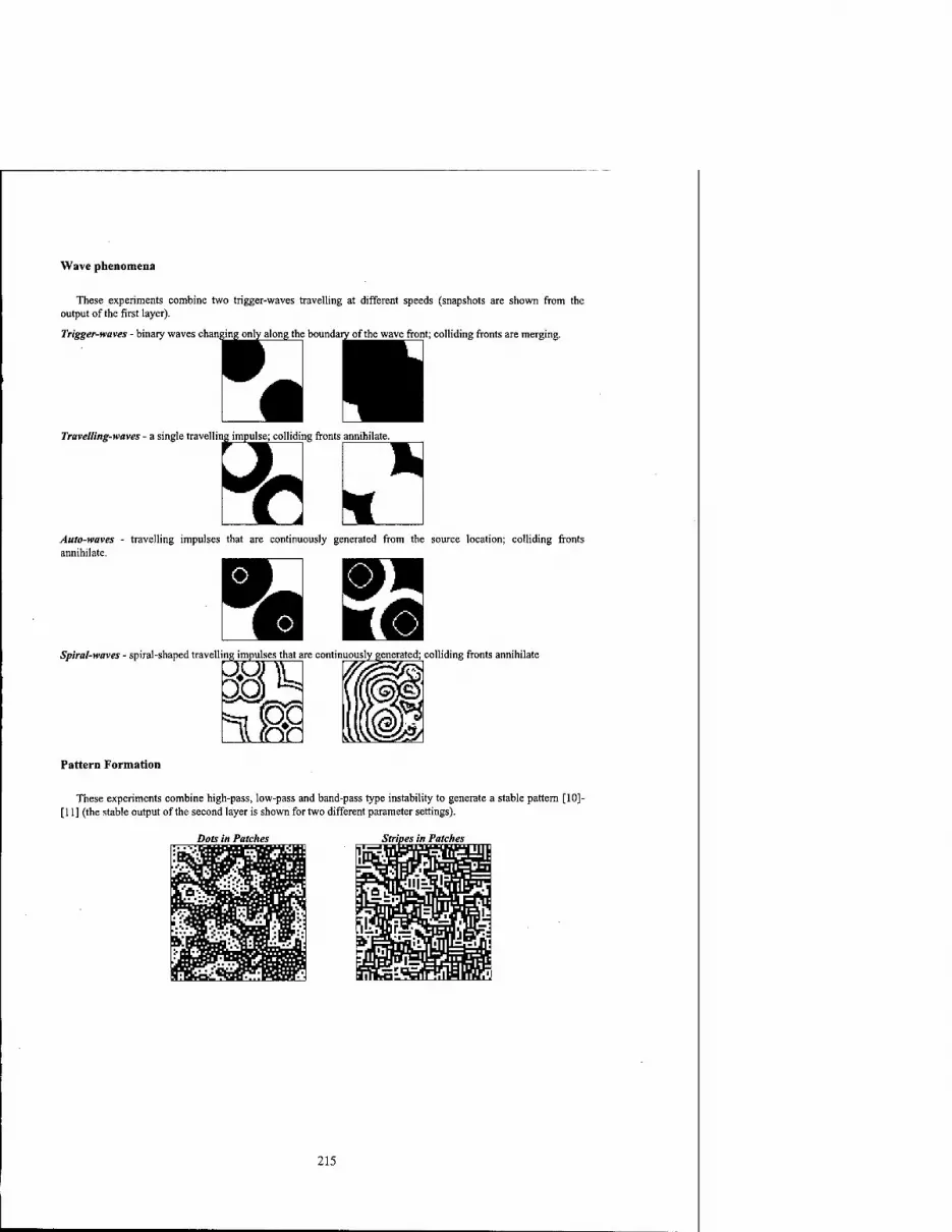
Wave phenomena

These experiments combine two trigger-waves travelling at different speeds (snapshots are shown from the output of the first layer).

Trigger-waves - binary waves changing only along the boundary of the wave front; colliding fronts are merging.

Travelling-waves - a single travelling impulse; colliding fronts annihilate.

Auto-waves - travelling impulses that are continuously generated from the source location; colliding fronts annihilate.

Spiral-waves - spiral-shaped travell are continuously colliding fronts annihilate

Pattern Formation

These experiments combine high-pass, low-pass and band-pass type instability to generate a stable pattern [10]- [11] (the stable output of the second layer is shown for two different parameter settings).

Dots in Patches Stripes in Patches

'ffiffiMFfc Wi-i- ML

Sffi

idln

X*

215

Image Processing

The 2n order sub-system makes it also possible to synthesize useful image processing operations by combining trigger-waves, diffusion and various filtering effects.

Halftoning - a gray-scale to binary image transformation that preserves the main features of the original image [12] (Observe that both layer outputs are halftoned images).

Original 1"layer layer

Smoothing and edge enhancement - a gray-scale to gray-scale image transformation that enhances the edges (see a comprehensive discussion on similar CNN based image processing methods in [13]). The architecture is neuromorphic, i.e. resembles the structure of the cone-horizontal system in the outer retina of the vertebrates where the horizontal layer is driven by the cones (Observe that the output of the first layer is a band-pass filtered while the output of the second layer is a low-pass filtered image).

Original 1" layer layer

Wave metric - a trigger-wave based method to measure the difference between objects [15] (Post processing: maximum detection on the output of the 2n layer).

1st object

Active Contour Detection - a combined diffusion and trigger-wave based method for identifying the contour of a labeled region [14] (Post processing: edge detection on the output of the 2"d layer).

Original Label (2"° layer ini) 1* layer

Edge and Skeleton Detection - morphological detection based on trigger-waves combined with high-pass effects (Remark: the edge and the skeleton is obtained for different parameter settings).

216

Original Edge (r layer) Skeleton( Is layer)

Summary

We have introduced and briefly discussed a 2nd order/ 3-layer CNN-UM architecture. It has been shown that a broad class of phenomena can be reproduced within the framework of this system. This motivates the synthesis of novel analogic CNN algorithms that can fully exploit the capabilities of this multi-layer CNN with stored programmibility. Details and chip design issues will be reported in forthcoming papers.

References

[I] L. O. Chua and L. Yang, "Cellular Neural Networks: Theory and Applications", IEEE Trans, on Circuits and Systems, Vol. 35, pp. 1257-1290, Oct. 1988.

[2] L. O. Chua, and T. Roska, "The CNN Paradigm", IEEE Trans, on Circuits and Systems, Vol. 40, pp.147-156, March 1993. [3] T. Roska and L. O. Chua, "The CNN Universal Machine", IEEE Trans, on Circuits and Systems, Vol. 40, pp. 163-173,

March 1993. [4] F. S. Werblin, T. Roska, and L. O. Chua, "The Analogic CNN Universal Machine as a Bionic Eye", International Journal

of Circuit Theory and Applications, Vol. 23, pp. 541-569, 1995. [5] B. E. Shi, "2D Steerable and Scalable Cortical Filters", in Proc. of the 7* International Conference on Microelectronics for

Neural, Fuzzy and Bio-inspired Systems, pp. 232-239, Granada, Spain, 19999. [6] B. E. Shi, "Gabor-type Filtering in Space and Time with Cellular Neural Networks", IEEE Trans, on Circuits and Systems,

Vol. 45, pp. 121-132,1998. [7] P. Arena, S. Baglio, L. Fortuna, and G. Manganaro, "Self-Organization in a Two Layer CNN", IEEE Trans, on Circuits and

Systems, Vol. 45, No. 2, pp. 157-162, 1998. [8] P. Arena, L. Fortuna, M. Branciforte, "Reaction-diffusion CNN Algorithms to Generate Artificial Locomotion", IEEE

Trans, on Circuits and Systems, Vol. 46, No. 2, pp. 253-260, 1999. [9] T. Serrano-Gotarredona and A. Rodriguez-Vazquez, "Implementation of Complex Dynamics Reaction-diffusion CNNs", to

appear in Journal of VLSI Signal Processing, 1999. [10] P. Thiran, K. R. Crouns'e, L. O. Chua, and M. Hasler, "Pattern Formation Properties of Autonomous Cellular Neural

Networks", IEEE Trans, on Circuits and Systems, Vol. 42, pp. 757-774, 1995. [II] K. R. Crounse, L. O. Chua, P. Thiran, and G. Setti, "Characterization and Dynamics of Pattern Formation in Cellular

Neural Networks", International Journal of Bifurcation and Chaos, Vol. 6, pp. 1703-1724, 1996. [12] K. R. Crounse, T. Roska and L. O. Chua, "Image Halftoning with Cellular Neural Networks", IEEE Trans, on Circuits and

Systems, Vol. 40, pp. 267-283, 1993. [13] K. R. Crounse and L. O. Chua, "Methods for Image Processing and Pattern Formation in Cellular Neural Networks", IEEE

Trans, on Circuits and Systems, Vol. 42, No. 10, pp. 583-601, 1995. [14] Cs. Rekeczky and L. O. Chua, "Computing with Front Propagation: Active Contour and Skeleton Models in Continuous-

time CNN", Journal of VLSI Signal Processing Systems, Vol. 23, No. 2/3, pp. 373-402, November-December 1999. [15] I. Szatmari, Cs. Rekeczky, and T. Roska, "A Nonlinear Wave Metric and its CNN Implementation for Object

Classification", Journal of VLSI Signal Processing Systems, Vol. 23, No. 2/3, pp. 437-448, November-December 1999. [16] S. Espejo, R. Carmona, R. Dominguez-Castro, and A. Rodriguez-Vazquez, "CNN Universal Chip in CMOS Technology",

International Journal of Circuit Theory and Applications, Vol. 24, pp. 93-111, 1996. [17] R. Dominguez-Castro, S. Espejo, A. Rodriguez-Vazquez, R. Carmona, P. Földesy, A. Zarandy, P. Szolgay, T. Sziränyi, and

T. Roska, "A 0.8 Um CMOS 2-D Programmable Mixed-Signal Focal-Plane Array Processor with On-Chip Binary Imaging and Instructions Storage", IEEEJ. SolidState Circuits, pp. 103-1026, July, 1997.

[18] S. Espejo, R. Dominguez-Castro, G. Linän, A. Rodriguez-Vazquez, "A 64x64 CNN Universal Chip with Analog and Digital I/O", in Proc. of 5th Int. Conf. on Electronics. Circuits and Systems ICECS'98, pp. 203-206, Lisbon, September 1998.

[19] T. Roska, P. Szolgay, A. Zarändy, P. Venetiäner, A. Radvänyi, and T. Sziranyi, "On a CNN Chip-Prototyping System", in Proceedings of 3rd International Workshop on Cellular Neural Networks and Their Applications CNNA '94, pp. 375-381, Rome, 1994.

[20] T. Kozek and T. Roska, "A double time-scale CNN for solving 2-D Navier-Stokes equations", International Journal of Circuit Theory and Applications, Special Issue on CNN II: Part I, Vol. 24, pp. 49-56, 1996.

217

2000 6TH IEEE International Workshop on Cellular Neural Networks and Their Applications Proceedings

Realization of Non-Linear Templates using the CNNUC3 Prototype

G. LXdn, P. Foldesy, A. Rodriguez-Vazquez, S, Espejo andR. Domlnguez-Castro

Instituto de Microelectromca de Sevilla - CNM-CSIC

Edificio CICA-CNM, C/Tarfia s/n, 41012- Sevilla, SPAIN

Phone: +34 95 4239923, Fax: +34 95 4231832, E-mail: linan@imse.cnm.es

ABSTRACT

This paper demonstrates theprocessing capabilities of a recently designed Analog Programmable Array Processor chip [1] - CNNUC3 - which follows the Cellular Neural Network Universal Machine computing paradigm [2] [3] [4]. Due to its very advancedfeatures and algorithmic capabilities, this chip has been demonstrated to be able to perform not only linear templates executions, but also to be very adequate for the implementation of non-linear templates by using a decomposition method. This paper focus on the application examples of the execution of non-linear templates with the CNNUC3 prototype. A brief description of the theoretical background is aho pre- sented in the paper.

1. INTRODUCTION

Cellular Neural Networks (CNNs) [2] exhibits outstanding image processing capabilities. They are capable to realize linear as well as nonlinear operations by using either linear or non-linear templates. Linear templates corre- spond to the case where interaction strengths (weights) are independent of signal values. Non-linear templates cor- respond to the case where interaction strengths depend on signal values.

Non-linear templates are needed for the realization of important image processing tasks. Techniques to imple- ment non-linearities using integrated circuit primitives are available elsewhere [5][6]. However, incorporating these techniques into CNN chips seriously compromises cell density. Actually, CNN chips reported to now are only capa- ble of establishing linear interactions. Still, piecewise-linear interactions can be emulated by taking advantage of the internal memory and the reconfigurability capabilities of last generation CNN-UM chips. Particularly, the so-called CNNUC3 chip [1] incorporates the following advanced CNN-UM features:

• capability to run algorithms with dozens of operations without external code or data movement;

• capability of storing four gray-scale and four binary images, on a pixel-by-pixel basis;

• capability to sum or subtract gray-scale images, also pixel-by-pixel;

• capability of selecting which cells are going to be processed (so called freezing map);

• capability to combine, pixel-by-pixel, two binary images through any user-selectable logic operation (such as logic "AND", "OR").

This paper experimentally demonstrates that these capabilities can be exploited for the realization of piece- wise-linear templates based on the algorithmic methods presented in [7]. The paper is organized as follows; Section 2 establishes a theoretical background about the technique of non-linear templates decomposition. Section 3 describes some applications examples. Some additional comments are provided in Section 3.4. Section 4 deals with the implementation of arbitrary non-linear functions. Finally, the conclusions are presented in Section 5.

2. DECOMPOSITION OF NON-LINEAR TEMPLATES

Implementing a piecewise-linear template by decomposing it into several linear ones is not a new idea. It has been previously studied in [7] at the algorithmic level. However, until now such implementation has never been demonstrated using actual CNN chips. As in [7], his paper deals with the case where only the B template is piece-

wise-linear, and assumes that the template is a 3 x 3 one.

CNNUC3 employs the so-called FSR CNN model [8] where cell dynamic evolution is given by:

t. This work has been partially funded by ONR-NICOP N68171-98-C-9004, DICTAMIST-1999-19007 and TIC 990826.

0-7803-6344-2/00/$10.O0 ©2000 IEEE 219

'»«WH B, C(i, I) e Sr(i. ft

gUijC)]

mL ,JTiy(/)<-l

0 ,|xy(«)|<l

C(k,l)eSr(i,j) i. i*. I (1)

(2)

(3)

(4)

where entries of the B template are linear.

Let us consider now that these entries are non-linear, namely,

where a and ß are real numbers. Let us define,

^ = a-«y + ß-uu

and assume that y© is a piecewise-linear function with m breaking points {t^, £2 i,m). Then, as demonstrated in [7], the non-linear template can be decomposed into a sequence of linear ones by using the algorithm described below [7].

• The process starts by selecting the first linear region of the non-linear function. Let us call R, this region that

is defined by the breaking points I;,, t,2.

• The next step is to select which are the cells belonging to that region. This calculation is realized by two tem- plates executions and a logic operation (all of them are done on-chip). With the first template, the so called threshold template, we drive to black all those cells having t, > ^, while with the second one, the so called

inverse threshold, we drive to black all those cells having (, < i,2. Finally a logic AND operation of both results

will select those pixels where ij, < I, < %2 *.

Equations (5), (6), show the threshold and the inverse threshold template**.

poo B=o«n z = -^i

0 0 0

0 1 0

000

poo 0 a 0 0 0 0

(5)

0 00 -ß 0 0 0 1 0 B = 0 -a 0 0 0 0j 0 0 0

12 (6)

• The non-selected cells are "frozen", by using the freezing mask provided by the chip, while in the selected ones the corresponding contribution to the state equation is evaluated and stored as a "bias map" that will be updated (or not) in the next iteration by adding the new result to the one that was previously stored. The updat- ing law for the state variables of the cells that are selected must be given by the equation of a straight line (due to the fact that M*© is linear between each two breaking points) crossing the points (,, and ^2. All the points

belonging to this line satisfy:

$-$! T(4)-4'(^)

$2-Si Vdy-H-Ci,) (7)

And from the CNN theory, it can be demonstrated that this relationship is obtained if the following template is

executed**:

t. Keep in mind that £, = a ■ u» + ß ■ uu and the subindcj kl denotes the cell' neighbours.

tt- These are the FSR version of the templates. In order to get the original Chua-Yang template increase by one the self-feedback term.

220

0 0 0 0-10 B =

0 0 0

fcß 0 0 0 i-o 0 0 0 0

where,

z = 4»(^)-t-5i

«Hfly-H»«,)

«2-5l

(8)

(9)

• The process continues for the next linear region.

• Finally, a template execution is needed. In this template the feedback term is the same as in the original one defined in (1), the feedforward term is set to zero (modified B template), since it has been already calculated, and the offset term is the addition of the original one z, and the "bias map" that is stored in some memory at the cell.

3. APPLICATION EXAMPLES

3.1 Absolute Value Calculation

Fig. 1 shows the corresponding templates and non-linearity. Because the transformation is pixel-wise - B tem- plate has 1 x l size - the decomposition method can be simplified, precluding accumulation of partial results. Besides, sub-interval selection reduces to estimating sign of the input and can be accomplished by using threshold templates,

(10) 000 0 0 0

020 B = OaO

0 0 0 0 0 0

particularly where a = 1, ß = 0 and 5, = 0. Since there are two sub-intervals, the number of cell maps is also two. The first one contains black pixels at the cell positions where the corresponding input image pixels are negative, and the second is the opposite. As a special case, the first transformation is equal to inversion and the second one can be avoided in practice since it lets the cells unchanged at their original values. Fig.2. shows the result of the execution of the absolute value calculation on CNNUC3.

[l] B = 0 0 0 0 ¥(5) 0 0 0 0

z = 0

Fig. 1: The absolute value calculation template.

3.2 Gradient Calculation

.The gradient template is defined in Fig.3. This template contains eight non-zero entries each of which has two possible intervals. Thus, the decomposition method results into a total of 32 linear template executions and thresh- old functions.

it. The position of the ß coefficient must be rotated in order to perform this operation for each of the neighbours of the cell appearing as a

non-linear connection on the original B template. Therefore, each linear region could require up to 16 templates and 8 logic operations to be

selected, 8 templates to update the state variable, and 8 templates to perform the addition of the results, that is 32 templates and 8 logic operations.

221

(a) Input (b) Absolute value

Fig. 2: The absolute value calculation.

A=[,] B = <V(t,) V(§) v&)

<F«) «Pß) *P«)

z = 0

Fig. 5: 77w Gradient calculation template.

The thresholded gradient operation is similar to the previous. The only difference is a shifting in the offset term.

Thus, the black pixels in the output image correspond to the input locations where the absolute value of the gradient is larger than z,hmhold.

Fig.4 show measurements taken from CNNUC3 which demonstrate the implementation of both gradient and thresholded gradient templates on silicon.

(a) Input (b) Gradient (c) Thresholded gradient

Fig. 4: The Gradient and Thresholded Gradient Calculation Templates.

3.3 Contour Detection on Gray-Scale Images

Fig.5 shows the associated templates and non-linear- ity. The result of this operation is an image having black pixel at those locations where the corresponding input is larger than some of the neighbours by a certain amount - 0.1 in the case of Fig.5.

Both the number of used mask generating templates

and transformation templates are 161"ft. Fig.6(b) shows the result of executing this non-linear template on CNNUC3 with the input image of Fig.6(a).

[2]* = <P($) ¥($) V(l)

_<F($) <P($) *P($)

z = -0.5

fF(S) +1

"ij-'u +0.1

Fig. 5: The contour Detection Template.

222

(a) Input (b) Detected contour

Fig. 6: Contour Detection on Gray-Scale Images.

3.4 Additional Comments

This section contains some additional ideas about decomposition, which are intended to reduce the number of required operations. This reduction is made possible due to some special functions incorporated to the CNNUC3 chip.

• If the number of intervals is only two, the "freezing" masks are opposite. Hence, the calculation of the second mask through template execution can be replaced by a logic operation.

• There are special cases where the general method can be modified in order to get a more efficient decomposi- tion. Specially, when the partial results contains only B&W pixels.In those cases, the generated interval maps contain all the information about the partial results. Moreover, when the final result is the logic sum (operation OR) or logic product (operation AND) of the partial outputs, the final result can be accumulated by the Local Logic Unit (LLU) in a Local Logic Memory (LLM) instead of by using the gray-scale accumulation process in an analog memory.

4. IMPLEMENTATION OF A GENERIC NON-LINEAR FUNCTION

The above described decomposition method can be used for piecewise-linear approximation of general non-lin- ear entries 1P(a utj + ß ■ utl) taking advantage of the fact that CNNUC3 is capable to distinguish 20 breaking

points within a characteristic curve. Assume that the non-linear coefficient can be approximated by:

19

F(K)'-

where,

"(£,) $20

otherwise

q-[«(^+i-ö-«ft,-öi

(13)

(12)

Then, the decomposition method can be applied to implement the approximated the function.

Another technique consists of approximating the non-linear func- tion into a stair-steps type non-linearity. In this case, the non-linear function is sampled at N points (up to 20 different in CNNUC3), and approximated by:

ttt. See that the number of required templates is not 64 as it should correspond to the case of having 8 non-linear connections. This is ex-

plained by the fact that the linear regions have an infinite or zero slope, and so, the linear transformation defined by (8) is not needed.

223

i = 0

(14)

To illustrate this technique we have implemented the following non-linear cubic-type function, considering an approximation containing 12 sampling points.

(15)

Fig.8(a) shows the result of the simulation of this template while Fig.8(b) shows the result provided by the CNNUC3 prototype. The input image has been already displayed in Fig.2 (a). Due to the sampling process, the out- put image needs post-processing - low-pass filtering also implemented by the chip - for proper signal reconstruc- tion.

(a) Simulated (b) By CNNUC3

Fig. 8: Cubic Template Execution

5. CONCLUSIONS

The executions of non-linear templates define an important application area in the field of image processing. However, previous VLSI CNNs implementations did not provide to the template engineers sufficiently accurate and versatile features to map the non-linear-to-linear existing algorithms. This paper presents experimental evidences about how a wide set of non-linear templates can be executed with by using CNNUC3. We have also briefly outlined the general decomposition method for implementing non-linear-to-linear template transformations in [7].

6. REFERENCES

[1] G. Lilian, S.Espejo, R. Domfnguez-Castro and A. Rodriguez-Vazquez-, "The CNNUC3: An Analog I/O 64 x 64 CNN Uni- versal Machine Chip Prototype with 7-bit Analog Accuracy". Proc. of the CNN2000, submitted.

[2] L.O. Chua and L. Yang, "Cellular Neural Networks: Theory". IEEE Trans. Circuits and Systems, Vol. 35, pp. 1257-1272, Oct. 1988.

[3] T. Roska and L.O. Chua, "The CNN Universal Machine: An Analogic Array Computer". IEEE Trans. Circuits and Systems II, Vol. 40, pp 163-173, March 1993.

[4] L.O. Chua and T. Roska, "The CNN Paradigm". IEEE Trans. Circuits and Systems I, Vol.40, pp. 147-156, March 1996. [5] A. Rodriguez-Vazquez, M. Delgado-Resrituto, J.L. Huertas and F. Vidal, "Synthesis and Design of Nonlinear Circuits".

Chapter 32 in The Circuits and Fillers Handbook (W.K. Chen — editor), CRC Press, New-York 1995. [6] M. Delgado-Resrituto, A. Rodriguez-Vazquez and F. Vidal: "Nonlinear Synthesis using ICs". in Encyclopedia of Electrical

and Electronics Engineering (J.G. Webster — editor), John Wiley & Sons 1999. [7] L. Kek and A. Zarandy, "Implementation of Large Neighborhood Non-Linear Templates on the CNN Universal Machine".

International Journal of Circuit Theory and Applications. Vol.26, pp. 551-566, 1998. [8] S. Espcjo, R. Carmona, R. Domfnguez-Castro and A. Rodriguez-Vazquez: "A VLSI-Oriented Continuous-Time CNN

Model". International Journal of Circuit Theory and Applications. Vol 24, pp. 341-356, May-June 1996.

224

2000 6™ IEEE International Workshop on Cellular Neural Networks and Their Applications Proceedings

Design of a dedicated CNN chip for Autonomous Robot Navigation

Mario Salerno, Fausto Sargeni, Vincenzo Bonaiuto

University of Rome 'Tor Vergata" Department of Electronic Engineering Via di Tor Vergata 110, 00133 ROME, ITALY

tel: +39 6 72597403 - fax: +39 6 72597401 E-Mail: sargeni@uniroma2.it

ABSTRACT: The obstacle avoiding is the main issue in autonomous robotics. It requires a three- dimensional effective environment sensing in real time. Among the others, the Stereo Vision approach to the environmental information extraction seems to be very appealing, even if it leads an extremely high computational cost. However, a high performance implementation of this algorithm on a Cellular Neural Network is able to overcome these difficulties. In this paper, the design of a new CNN chip well suited for this algorithm will be presented. This chip, performing a real time processing of the stereo vision data, will improve the cruising speed of a robotic platform.

1. Introduction

In autonomous robotics the three-dimensional information extraction for obstacle avoiding represents the most crucial issue. Several techniques are employed for the environmental sensing, with particular reference to the depth information with respect to the observer. Among the others, the algorithms based on Stereo Vision represent one of the more promising and reliable approaches. A stereo head, composed of two parallel TV cameras, acquires couple of images from two slight different points of view. A processing task of these couple of images that correlates the conjugate points on them, is able to reconstruct the three-dimensional information of the environment. On this purpose an effective implementation of this algorithm has been obtained by using the Cellular Neural Networks (CNN) [1-4]. By this approach, the problem of correlating conjugate points is implemented as an optimisation task, performed by a suitably programmed CNN. Moreover, the use of an analogue highly parallel hardware circuit will allow satisfying the real time requirement. In this paper, the design of a new CNN chip suited to implement this algorithm will be presented.

2. Recall of the Stereo-CNN algorithm

In order to evaluate the depth information in a 3-D environment, the stereo vision approach processes couples of images taken from two slight different points of view. So, the distance of an object in the scene can be estimated on the basis of the projection on the two images. The main issue is to properly match these projections across the two images. The idea, on which the Stereo-CNN algorithm is based, is to formulate the problem of stereo matching through a variational approach as the relaxation of an opportune energy functional. Through the comparison of this functional with the internal energy expression of the Cellular Neural Network (CNN), it is possible to derive the connection templates, which specialise the CNN to the resolution of the stereo matching problem.

The CNN are a class of artificial neural networks widely used in image processing and pattern recognition problems. They consist of a two-dimensional network of elementary analogue processor only locally connected. Their high speed analogue parallel processing feature makes them suitable in such a problem where a real time response to external stimuli are required.

The Stereo-CNN has to match pixels between two input images, an additional dimension is required in the network in order to take into account the disparity information. Such a network is thus composed of a number of layers (each of them of the same dimensions of the input image) determined on the basis of the optical and geometrical features of the used image system. In this way, each layer processes a different disparity. Through the above mentioned comparison the first neighbour connection templates and biases are derived. In order to assign a single value of disparity to a pixel location, we consider all the cells along the direction described by k. The value relative to a location will be 0 < k < D where k is the index of the plane where the steady output value of the cell is maximum, i.e.

0-7803-6344-2/00/$10.00 ©2000 IEEE 225

t:vyijf =™axl,'>,.M(00)]]

The existence of a Lyapunov function guarantees the stability of a CNN, and allows the possibility to use the CNNs for optimisation purposes. The basic idea is to express a problem in terms of a function optimisation. We compare such an expression with the energy function of the generic CNN and we find a particular instance of a CNN able to code the problem in its connectivity templates. Thus, operating the CNN built in such a way, we will solve the original problem we are interested in [5]. Reformulating the stereo matching problem in terms of a variational form [6] and using the above mentioned three-dimensional CNN, we can obtain the connection templates by which it is possible to code a stereo vision problem in a CNN.

A possible solution for this comparison it is represented by the following templates: A(i, j,k;l,m,n)= (l-r-2W)5, ,SJ mSk „ +U£ö{i m m)¥,Sk „

*5 (1) where 5,;- is 1 when i = j, otherwise it is zero, X is a trade-off parameter between the continuity term and

the luminance matching term in the variational expression for the stereo matching problem, t is a parameter ruling the speed of convergence of the network, W is linked to the dimension of the window of the CNN templates and S is an index set in this window excluding (0, 0) [1].

B(i,j,k;l,m,n) = 48ij8jm8k (2)

Where the constant is a needed normalisation term, according to the constraint on input values (see [2]), coming from the input voltage equation:

„ fa(u)-Mu+*y "u* 4

Moreover we have I = 0. The most important observation on the outcome of the approach is on the topology of the found network. In equations (1) and (2), because of the presence of term 5* „, it is evident that there arc

no inter-layer connections, each cell is linked to its neighbours in the same layer. Therefore each layer is physically uncoupled from any other. This greatly simplifies the architecture of the system, allowing the possibility to implement only one layer at a time. The layers arc coupled only logically through the computation of the maximum activation.

For example, a typical set of template is as follows:

'0.5 0.5 0.5 "|

0.5 -4 0.5

0.5 0.5 0.5

(0 0 °] 0 4 0 0

V 0 °J

1 = 0 (4)

3. The ASIC CNN chip

The basic idea of this project is to design a CNN chip able to compute, in analogue way, the disparity map from the vuijk values of eq. (4) which are related with the pixels of the left and right images. It is worth noting that no data exchange between the processor and this high performance analogue coprocessor is required and the whole disparity map will be computed directly into the chip. In fact, the designed circuit will be able to perform the algorithm with no analogue to digital conversions

The first step in designing of this new chip has been the architecture of a single cell. This architecture is composed by DPTA's (Digitally Programmable Transconductancc Amplifier) [7-9], capacitors, a comparator and logic registers. First of all, the implementation of the term B*Vu will be described.

This term of the state equation has been implemented by a 8-bit DPTA. The use of a single DPTA is required by the central term B22, which is the only entry of the matrix B different from zero. In addition, the input voltage Vu has to be computed by an external processor starting with the two left and right input images. This external processor will compute the expression of the formula (3) and the multiplication by the central term B22. This design choice has been done in order to simplify the analogue circuitry and to allow changing the equation (3) itself. In fact, the authors in [1,7] are trying different expression of this formula of the input voltages in order to obtain improved results.

The template A has been implemented by a Multiple-Outputs DPTA depicted in Fig.l. This circuit has been

226

designed with one output for the term A22 and eight equal outputs for the other entries. The programmability has been implemented only for the central term while the others are properly mirrored with a ratio of 8:1. This ratio is always constrained to this value and than it has been fixed in the design. Three bits are dedicated for this term. The layout is shown in Fig. 2. The size is 112x71 micron2.

The most interesting part of the chip is that devoted to the calculation of the minima state voltages. This calculation is required to be computed among different runs of the same cell. The minimum value of the state voltage of the same cell (i.e. the same pixel) detects the value of index of the disparity.

If you implement this computation by digital circuitry you need a lot of components as A/D converters, memory (sized NxNxP, if NxN are the dimensions of the CNN and P is the number of planes of disparity to be computed) and a processor to find the minima. This solution is very expensive especially with real-time constraints. A more effective architecture is now presented. In this architecture, no A/D converters are necessary. In fact, analogue circuits are used to perform all the computations to find the required disparity map.

Figure 3 depicts the CNN cell. There are two different branches connected to the same resistor and DPTA's. These two branches are made of switches and capacitors. Both the two capacitors are "state" capacitor and will be properly connected to the resistor with respect to the result of the previous transient (i.e. the capacitor charged to the minimum voltage). In fact, in the i-th transient, it is used the capacitor charged at lower voltage value. The switching between one branch or the other will be controlled by a comparator which compare the two voltages of the capacitors. One capacitor contains the previous steady-state state voltage, while the other capacitor contains the present state voltage. A digital counter will be used to increment the disparity index. Some logic gates are required in order to give a proper Enable pulse to a digital register to store the present disparity index. The occuped area of the cell is about 180x180 micron2. This small area will allow a 64x64 cells for the whole design.

The estimated time to compute a ten planes disparity map for a 64x64 pixels image is about 140microseconds.

The chip will be manufactured by using the AMS-CYE 0.8u.m technology (double poly and double metal).

5. Conclusions The artificial vision for robotic system is a very interesting topic to develop CNN approaches. In this fields,

some researchers from ENEA, presented a Stereo-CNN algorithm for the computation of the object distances. In previous papers, the authors designed and manufactured a system of 720 CNN cells that has been used to test the algorithm itself.

In this paper, a new CNN chip well suited for this algorithm has been presented. The use of this chip will allow using the stereo vision in practical robotic tasks with real-time analysis of stereo vision.

6. Acknolegments

This project has been partially funded by the Italian Ministry of Scientific Research (Projects PR1N-9809272019)

7. References [1] S. Taraglio, A. Zanela, "Cellular Neural Networks for the Stereo Matching Problem", Proceedings of the Fourth

IEEE International Workshop on Cellular Neural Networks and their Applications, CNNA-96, pp. 93-98, Seville, June 1996

[2] L. O. Chua, L. Yang, "Cellular Neural Networks: Theory" IEEE Trans. Circuits and Systems, Vol. 32, Oct. 1988, pp.1257-1272.

[3] L. O. Chua, L. Yang, "Cellular Neural Networks: Applications", IEEE Trans. Circuits and Systems, Vol. 32, Oct. 1988, pp. 1273-1290.

[4] T. Roska, J. A. Nossek (Eds), "Special Issue on Cellular Neural Networks", IEEE Trans, on Circuits and Systems, Vol. 40, no. 3, March 1993.

[5] A Zanela, S. Taraglio. "Sensing the Third Dimension in Stereo Vision Systems: a Cellular Neural Network Approach", International Journal on Engineering Applications of Artificial Intelligence, in press, 1998.

[6] T. Poggio, V. Tone, C. Koch. "Computational vision and regularization theory", Nature, 317, pp 314-319, 1985. [7] F. Sargeni: "Digitally Programmable Transconductance Amplifier for CNN Application", Electronics Letters, vol.30,

no. 11, May 1994. [8] M. Salerno, F. Sargeni, V. Bonaiuto, "6x6DPCNN: a programmable mixed analogue-digital chip for Cellular Neural

Networks", Proc. of CNNA-96 4* IEEE Int. Workshop on Cellular Neural Networks and their App, Seville, Spain, 1996, pp. 451,456.

[9] M. Salerno, F. Sargeni, V. Bonaiuto, "A 6x6 cells interconnection-oriented programmable chip for CNN\ Analog Integrated Circuits and Signal Processing, Kluwer Academic Publishers, Volume 15, no. 3, March 1998, pp.239-250.

227

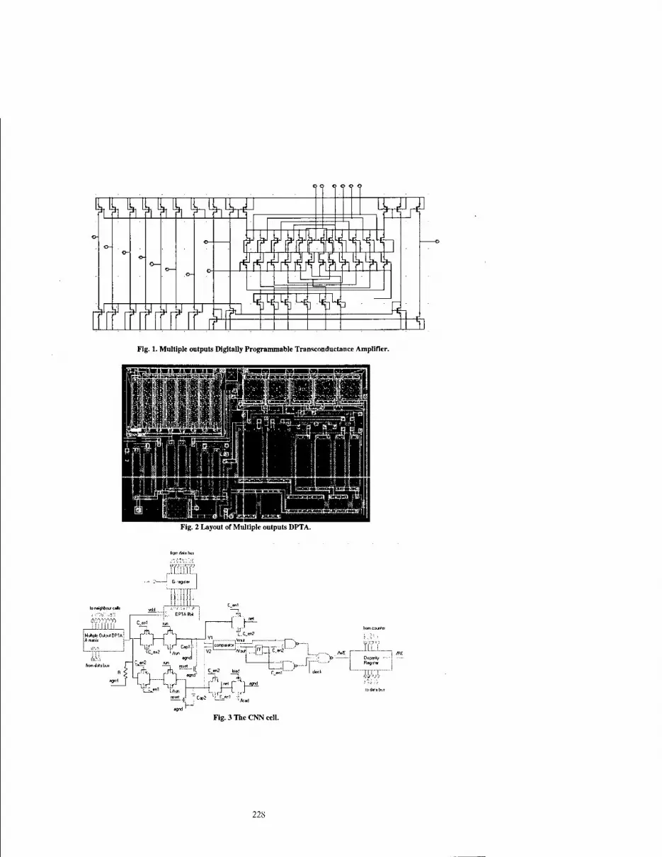
oo <> © © ©

LL tlUlL 1Ü

,f-i ril Vil Si VI I oWrr u m- I^LMJLI

Fig. 1. Multiple outputs Digitally Programmable Transconductance Amplifier.

Fig. 2 Layout of Multiple outputs DPTA.

II _LLLLUli_

"L.C_en2

-,VnJl .—

i ~S..,.,E

V2 W«,

C_en2 load

:« * Jf Regis'*

wyl ,;t " C*2 -; C„w,1

Fig. 3 The CNN cell.

228

2000 6™ IEEE International Workshop on Cellular Neural Networks and Their Applications Proceedings

A Compact Digital CNN Array for Video Segmentation System

Art Paasioi,2l Jani Paakkulainen1 and Jouni Isoaho1

1 Laboratory of Electronics and Information Technology, University of Turku FIN-20014, University of Turku, Finland

2Electronic Circuit Design Laboratory, Helsinki University of Technology phone: +358-2-333 6574 fax: +358-2-333 5070

e-mail: apa@ecdl.hut.fi

ABSTRACT: In this paper neui ideas are given for implementing a fixed template Cellular Nonlinear Network processor. Our concept is based on calculations in the digital domain so that the desired accuracy can be transformed into selecting appro- priate word lengths in different parts of the system. In this paper we concentrate on implementing a weighted average circuit that guarantees a true 7 bit accuracy in the processing.

1. Introduction

In [1] a concept, cellular neural network (CNN), suitable for image processing was introduced. According to the original idea in [1] the processing is performed with analog circuits. Also, some digital CNNs have been introduced [2, 3]. In this paper another digital approach is suggested, where the programmability has been abandoned, and only a fixed task needs to be performed. By fixing the task a very compact design can be achieved from the layout area point of view.

In this work we concentrate on a specific gray scale image processing task, a constrained two dimensional low-pass filtering. The filtering is the only gray scale processing task with linear templates in a CNN algorithm for video image segmentation in [4] and therefore the design in this paper can be considered to be implemented on the same substrate with the design in [5]. This paper concentrates more on the evaluation of the weighted spatial average given by the B-tempIate, and another paper [6] focuses on the realization of the A-template. Therefore, the details concerning the integration, i.e. the evaluation of the A-template, are only briefly given here.

2. System design issues

The requirement of the system is to evaluate a template

0.1 0.1' / = 0 (1)

with a gray scale image of size 176 x 144 pixels. The accuracy of the input is a standard video image accuracy eight bits per pixel. The system can be considered to be realized by two separate blocks. Namely, one block is dedicated for evaluating the weighted average of the neighborhood, the weights being given by the B-template. The other block handles the integration required to realize the performance given by the A-template.

2.1 Processing region

In the original CNN the input image is bounded between the values -1 and +1. To make the hardware more simple, the image can also be transformed linearly in such a way that the values are between 0 and +1. This transformation to positive range has been described e.g. in [7]. Now the eight bit image information can be represented so that a value 0 corresponds to a white pixel and a value 255 corresponds to a black pixel. Positive range is chosen mainly because it makes the actual cell structure simpler [6].

0 1 ol 1 -4 1 S = 0 1 0

0.1 0.1 0.1] 0.1 0.2 0.1 0.1 0.1 0.1

0-7803-6344-2/00/$10.00 ©2000 IEEE 229

2.2 Processing strategy

The processing of the image is designed to be performed in such a manner that only a fraction of the image is processed at a time, i.e. the image is divided into smaller areas which are evaluated individually. To still obtain correct results an overlap large enough has to be allowed for the sub-images. This requirement is explained in more detail e.g. in [8] for this particular template. According to the results in [8] we require an overlap of 12 pixels in the image when the actual cell array is concerned. If only the B- template contribution is calculated, then it is a well known fact that we only have to guarantee the full 1-neighborhood for the pixels under evaluation. Because the effect of the B-template is to introduce a space-variant constant to the processor cells, the magnitude of that bias has to be evaluated only once for every sub-image. The strategy for implementing the low-pass filter is shown in Fig.l, where the image is loaded from an input image buffer to a unit where the evaluation of the B-template is performed. The loading is done in a row-by-row manner that is well suited for the evaluation of a simple B-template. The dimension of the B-template block is thus 176x1, and it contains memories to guarantee a real 1- neighborhood for the cells. The results from this block are then written to the cell array in a row-by-row fashion. The dimension of the cell array is 176xN, where N is 144 or smaller [6].

INPUT IMAGE BUFFER

B-TEMPLATE EVALUATION

CELL ARRAY

-«—176 cells —»•

Figure 1: Different low-pass ßter building blocks.

2.3 Multiplier-free realization

The realization of the cell for the evaluation of the A-template, where no multipliers were used was introduced in [6]. The multiplications were realized by shifting operations corresponding to multiplications by the power of two. In calculating the contribution of the B-template dedicated multiplier structures could be considered. However, also this part of processing is easily performed by adding only few shifted versions of pixel values together. This can be done without sacrificing the accuracy and it greatly reduces the required layout area.

Here, two different B-templates that have their entries built from the sums of powers of two are proposed. The influence of the accuracy of the B-template elements to the overall processing result is achieved by comparing the final processing result to a result obtained when using floating point representation for 0.1 and 0.2 in the multiplication. Here, we follow the cell realization given in [6] with the internal word length 11 bits. This cell is also briefly described later in the text.

The templates used in the simulations were of form

(2)

230

where a and 6 consist of either three or four sum terms. With the first B-template (Bl) and with three terms the values for a and 6 are chosen to be 0.09765625 and 0.21875, respectively. If we allow an additional fourth term then o equals 0.099609375 and 6 equals 0.203125. This second B-template is denoted by B2. Note that in both cases the condition 8*a + 6 = lis fulfilled. The powers of two that are used in the templates are listed in the table below.

Bl o = 2-4 + 2-" + 2-8

6 = 2"3 + 2"4 + 2"5

B2 a = 2"4 + 2"5 + 2-" + 2"" 6 = 2"3+2-4+2-6

The first result from the simulations was that making the result of the B-template evaluation more accurate than 11 bits, that being the accuracy in the evaluation of the A-template, does not increase the overall accuracy. By using the same evaluation criteria as in [6], where the accuracy of the result is log2(128/DEV) and DEV is the maximum pixel value deviation from the 'ideal' result, we get the second result. According to our simulations we achieve 7.265 bit accuracy if the multiplications in the B-template are performed with floating point accuracy. If we use template Bl the accuracy is 7.06 bits where the accuracy with the B2 template is 7.25 bits. In the next chapter we describe the hardware designed for evaluating the template Bl. This template ensures true 7 bit accuracy.

3. Digital circuit realization

3.1 Processor cell for iteration

The block diagram of the cell that is used to make the integration is shown in Fig.2. In the system the integration step has been chosen in such a manner that it preserves the original functionality but the only multiplication of the cell values, i.e. the state and BETA, is a multiplication by 0.125. This multiplication is easily achieved by shifting of a binary number representation and therefore a totally multiplier-free cell structure has been achieved. A more detailed description of the circuit is in [6].

mOMNEXlHBOfl

Figure 2: Digital cell block diagram.

The cell contains one adder and registers to store the present state, the space variant cell bias BETA and intermediate results of the integration. Moreover, there is a multiplexer to select the term to be added.

3.2 Evaluation of BETA

The block diagram for the Bl-template evaluation is shown in Fig.3. We denote the result of the calcu- lation by BETA. Because the evaluation of BETA is performed one row at a time, and because there are only 176 units like the one described here more hardware can be dedicated for this procedure than for the integrator cells while still keeping the total layout area within reasonable limits. The circuit for the B-template evaluation consists of three different building blocks. Namely, there are adders, registers and shifters, where actually the shifting operation can be performed by hard wiring.

The calculation for BETA can be considered to be performed in three phases. In the first phase the input is multiplied by four different terms, in this case four different shifting operations are performed. These shifted terms are added so that at end of stage one there is the input multiplied by 0.21875 and 0.09765625 in two separate registers. These points in the data flow are denoted by A and B in Fig.3,

231

respectively. In phase two, the term representing value 0.1 is sent to the left and to the right neighbor blocks. Then, an adder counts up two terms coming from the neighboring cells and this sum is again added to the values that exist at points A and B. The results are denoted by C and D in our block diagram. The path of C now contains terms that are located in the middle row of the B-template. The data in path D is required to evaluate the'contributions from the upper and from the lower rows. Because the image data comes to the input register one row at a time, delays have to be added to the data paths properly in such a way that correct row information existing at C and D at some time are added up correctly. This is done in the last phase where the data in point £ is a delayed version of D and thus the data in E represents contributions from the pixels that are located in the row above. When terms C and E are added, a sum consisting of six terms, namely of the top and the middle row elements in the B-template, is obtained. This value has to be delayed (point F) in such a manner that the remaining contributions from the row below the pixel reach data point G, which is a copy of contents at point D. The correct value in G is of course only valid if we have written the pixel information of the next row to the input register and have allowed the corresponding data to propagate through the network. The sum of F and G is our result BETA, which is then written to the processor cells. It has to be noted that special care has to be taken when the active row to be evaluated is either the first or the last in the original image. This is important so that proper boundary values can be assigned to the corresponding registers at a proper time. This procedure is, however, not described here in detail.

4. Conclusions

An alternative method for realizing a fixed template CNN hardware has been given. The digital processing offers accuracy possibly not easily reached with analog approach. The reported design is a part of a constrained low-pass filtering, the only gray-scale CNN task with linear template elements in the targeted application. This design used together with a full QCIF size B/W CNN Universal Machine core offer a promising solution for video image segmentation.

Acknowledgments

This work is supported by the Academy of Finland (#1168301/00) and (#1366361/99).

References

[1] L.O.Chua, L.Yang, 'Cellular Neural Networks: Theory', IEEE Transactions on Circuits and Systems, Vol. 35, pp.1257-1272, 1988.

[2] A.Zarandy, P.Keresztes, T.Roska and P.Szolgay, 'An Emulated Digital Architecture Implementing the CNN Universal Machine', Fifth IEEE International Workshop on Cellular Neural Networks and Their Applications CNNA'98, London, U.K., pp.249-252, 1998.

[3] S.Jankowski, R.Buszynski, A.Wielgus, W.Pleskacz, T.Szoplik, I.Veretennicoff and H.Thienpont, 'Digital CNN with Optical and Electronic Processing', European Conference on Circuit Theory and Design ECCTD'99, Stresa, Italy, pp.1183-1186,1999.

[4] A.Stoffels, Titoska, L.O.Chua, 'Object-Oriented Image Analysis for Very-Low-Bitrate Video-Coding Systems Using the CNN Universal Machine', International Journal of Circuit Theory and Applica- tions, Vol. 25, pp.235-258, 1997.

[5] AJPaasio, A.Kananen, K.Halonen and V.Porra, 'A QCIF Resolution Binary I/O CNN-UM Chip', Journal of VLSI Signal Processing Systems for Signal, Image and Video Technology, Vol. 23, pp.281- 290,1999.

[6] A.Paasio, J.Paakkulainen, J.Isoaho, 'A Multiplier-Free Fixed-Task Digital CNN Array for Video Segmentation System', Proceedings of ISC AS 2000, Geneva, Switzerland.

[7] A.Paasio, 'Integration of Cellular Nonlinear Network Universal Machine', Ph.D. dissertation, Helsinki University of Technology, Espoo, 118 pages, 1999.

[8] A.Kananen, A.Paasio, K.Halonen, 'Overlapping issues in designing large CNNs', Proceedings of CNNA 2000, Catania, Italy.

232

VTTV-1

tojeft

from_left -

^

in V7 VY

to_rlght

from_right

y, I I

I

Figure 3: B-template evaluation block diagram.

233

2000 6™ IEEE International Workshop on Cellular Neural Networks and Their Applications Proceedings

Application of Time-Varying Cellular Neural Network for Optimal Solutions

Nasser Kamiss Al-Ani and Tomasz Kacprzak Technical University of tödi Poland

Institute of Electronics, Stefanowskiego Street 18/22, 90-537 tout, Poland e-mails: Nasserkhm@hotmail.com, kacp45@sg-ck.p.lodz.pl

ABSTRACT: A Time-Varying Cellular Neural Network (TVCNN) with a new scheme of annealing is proposed for finding the global optimal solution of multivariable cost function. The technique is an engineering annealing method, which is the advanced electronic version of mean-field annealing. The processing of finding the global minimum of the generalized energy function is implemented, by first increasing the energy level by reducing the voltage gain of neurones. Then searching for the global minimum energy level by increasing the neurone gain. The process of the global optimization will be explained by the system eigenvalues with two computer simulation.

1. Introduction

A Cellular Neural Network (CNN) is a nonlinear locally interconnection analog processor array arranged in two - dimensional of «-rows and m-columns. The network parameters for invariant CNN are given in a template set, consisting of the feedback matrix A, control matrix B and network bias /j . The basic dynamic equation can be described by N = nxm non-linear differential equations:

Cx -^-^-^-Vxij + AVyU+BVrt, +Ib 0)

Where the state vector Vx=[vx, v^ W|T, the output vector Vs = [vs, v!2... v,nf, and the input vector Vu = [v.i v„2 ... VM]

1. The nonlinearity is in the piecewise-linear (PWL) equation. The Lypunov energy

function of a CNN with (PWL) is given by:

E = .-LvjMV -Vfk (2)

where M=A - Tx I, b = Bu + Ib W, and W = [1 1 1]T is a unit vector (1*N). Generally a CNN operates by choosing a template set A, B, h and appropriately assigning the initial state. Then, the desired output can be obtained as a stable equilibrium of the system (1) [1,2]. When the neurone gain g(t) is changed from very smal value up to unity, in a manner equivalent to decreasing the temperature in simulated annealing, a Time Varying Cellular Neural Network (TVCNN) is performed. This method was introduced by [2,3] and extended by [4, 5,6]. Under this condition of operation the transfer function of the cell can be described by:

v^=/(g(/).v^W) =

+ 1 g(t).Vxij(t)>l

g(t).vxlj(t) -\<g(t).vxijU)<l (3) -1 g{r).v^.(/)<l

The Lypunov energy function of the TVCNN is defined as:

£=-jF/ (A-^-I)Vy-Vl b = -jVyTMg Vy -V

Tyb (4)

0-7803-6344-2/00/S10.00 ©2000 IEEE 235

Since the matrix Mof (2), is symmetric, all its Xk (k:l..N) are nonnegative [7]. For Xk>0; Vk, there will be a stable node equilibrium state y0 =Hf'b, to which the network will converge. When the cell gain g varies with time, the system matrix will be time varying function which will result in eigenvalues bing time varying also. The finding of the optimal solution can be understood by observing the eigenvalues of the time varying matrix Mg throughout the time evolution. By noting that {Mg = A-TJ-((l- g)T/g)I =M-((l-g)TJg) I}, the relation between the eigenvalues of invariant and varying cell gain networks can be easily shown to be:

Xk(t) -*\- Q-g('))r, k=l,2 ,N. (5)

Where /lk's are the eigenvalues of Mg and A.k'"s are the eigenvalues of M. The initial cell gain g„ must be very small positive value (s), such that the eigenvalues change gradually from all negative initial values to final values V by increasing the gain from s to 1, in the same time the energy function (4) which is initially a convex function of Vy, is transformed gradually into a concave function. For each value of g, there is a set of eigenvalues Xk and equilibrium pointy« =-Mg'b. For the initial values of g {g =e }, both initial output y(0) and the equilibrium y0are close to the origin and y(0) = yo(0), because {y = f (go.x) = go.x = 0}. In other words there exist only one equilibrium point belongs to the centre region of the CNN, where all cells work in the linear part of their characteristic. Such a point is stable and its basin of attraction is the whole space of state. By increasing the cell gain g for g <, gc , Eq.6, the network movement is within the linear region with only one stable equilibrium point. The Xk''s are still negative, that allow the network to change its state to the new stable equilibrium point [8, 9], The movement of the network for 0 < t <tc can be denoted as y(g). The increasing rate of g must be achieved carefully, such that for I <lc, the matrix Mg is definite negative, at which the annealing process can force the network such that the output moves toward the basin of attraction for the global minimum of the energy state. Then by increasing g from e to 1, Fig.l, y(g) remains the only equilibrium point of the system. Two gain values are very important in the annealing operation. First the critical gain gc, before which the network must take enough time to reach the basin of attraction to which the optimal minimum of (4) belongs. Second is the saturation gain g5, beyond which all saturated binary outputs are guaranteed. In (5), the first positive eigenvalues results when the applied gain is:

Tx £ = ± 2 4- T "• maxT Lx

Tx -, i.e. gc> - c 2 j. T A max^ Ix (6)

According to that a modification of the applied time-varying control signal gain was proposed and tested [4], with save in time about 40% compared to that in [3].

2. Experimental Networks

To see the properties of the TVCNN procedure of optimal solution, we analyse two experiments. The proposed scheme of annealing is shown in Fig.l.

2.1 Three-cells network In this section a three-cells circular network, Fig.2, will be tested with the template parameters, feedback template-/!, feedforward template-B, and bias-/4 as following:

^ = [-0.25 2 -0.25] ,ß = [0 1 0],/j=0 (7) Fig. 1: The applied gain as proposed in [4].

The energy function, Eq.4, can be simplified for the three-neurones network as:

236

E=-^[yt yi y*]

T'/ -.25 -.25 /g V\

.25 >"% -.25 yi -

.25 -.25 T / 2- 'A\ UsJ

1 0 0 0 1 0 0 0 1

(8)

y' ^ < "y2 ^<^S vy3

Fig. 2: The full connection of the three cells circular network.

For input vector U= [-.2 -.5 .3 ], the network has 8-equilibrium points. These equilibrium points are stable and have a transient state values as following: E,(1.3, 1,1.8), E2(-2.2, -2.5,2.8), ^{-2.1,1.5,2.3), E4(1.8, - 3,2.3), E5(1.8, 1.5, -2.2), E^-U, -2, -1.2), £,(2.3, -2.5, -1.7), and EsC-2.2,2, -1.7). Fig.3 shows the plot of the two dimensional energy surface as a function of output state vector Vy. The Fig.3a, is for the first four equilibrium points when the output state of cell-3 is 1 (high) and the Fig.3b is for the last four equilibrium points when the output state of cell-3 is -1 (low). The figure shows that all corners (equilibrium points) are possible minima depending of input and initial states. The network with time-invariant cell gain (gft) is constant of 1) is tested for different initial state. The trajectories of these different tests are shown in Fig.4a.

E,(l,l,-1)

l Output Cell-1 Output

(b) Fig.3: The network energy surface: a) The first four equilibrium points, b) the last four equilibrium points.

(£)V

| 1 -2

\ 1 ! 1 b

V-'j \ i e

ik-.i i \ i-f-

\\ i i 1 ~sj i i i 9 c

l\ ' ' ' \\l • : d

XX' \\ ■ i a n

Cell-1 State Voltage i 6 Tnre

2 V

(a) (b) Fig. 4: The network with time-invariant cell gain, a) the network test for different initial state denoted by

a,b,..,i, b) the corresponding energy function of time.

237

The energy evaluation for the tests (a, b, ...,i) are shown in Fig.4b. The network has different energy level with the different output dynamic equilibrium points. The lowest energy level is (-2.75) with the equilibrium point E2. The above network is tested with time-varying cell gain for the same initial state values that are denoted in Fig.4. The trajectories of these tests are shown in Fig.5a. The figure shows how the TVCNN attracts the network at 1(0) to the centre of the output dynamic space for all these initial states, then it moves slowly in the linear region (search phase) searching for the basin of attraction of the optimal solution (the lowest level of the energy function). For all these tests, the network is terminated in the saturated region of the equilibrium point E^-l, -1,1), in which the energy function has lowest value. The above simulation shows the ability of TVCNN to get out of local minimum and to converge to the global one. The energy evaluation of these different testes are recorded in Fig.5b, which are at the same energy level of (-2.75).

-15

•!

-25

-3,

-0.5 o' 0 5' Cell-1 output vyl

(a) Fig.5: The network with time-varying cell gain test, a) the network convergence from the different initial

state (a,b,..,i) to the equilibrium point E;, b) the corresponding energy function evaluation

i : :

1 ^

I \ tib,<;..4l ;..\; •

j > i

| %-

Tire

0>)

2.2 Sixteen Cells Network: In this section a 2-dimensional sixteen-cells network will be tested with the template parameters, feedback template-^, feedforward template-B and bias-/j as following:

A =

0 -.25 0 ' "0 0 0"

25 2 -25 , B = 0 1 0

0 -.25 0 0 0 0 /»=o (9)

The network feedback system matrix A and the feedforward system matrix B are eNxN, where N is 4x4, and the input vector Vu e lxN. The network has thousands of equilibrium points in its output dynamic space. Some of these equilibrium points are stable and the others are not. Fig.6 shows the plotting of the two dimensional energy surface as a function of output state vector Vy!! and Vy23. The figure includes four equilibrium points two of them are unstable, E3 and E4 while the other two E2 and E]are stable. The global minimum of Eq.4 is with E,, while the energy is local minimum with the other equilibrium points including

All corners of the energy surface with stable equilibrium points are possible minima for the network with time-invariant CNN, depending of input and initial states. From an initial state the network is tested for both time-invariant and time-varying CNN. Fig.7 shows the time evolution of the energy function evaluation. The network with time-invariant cell gain converges to the equilibrium point that shown in the Fig.7 with energy level of (-10.1). The network with time-varying cell gain is tested from the same initial point that of time- invariant cell gain and it terminates with the equilibrium point E]. The test shows how the network escapes from the local minimum that the network reached in time-invariant CNN and converges to the global one (energy level of-14.7). The trajectories of these tests are shown in Fig.8.

238

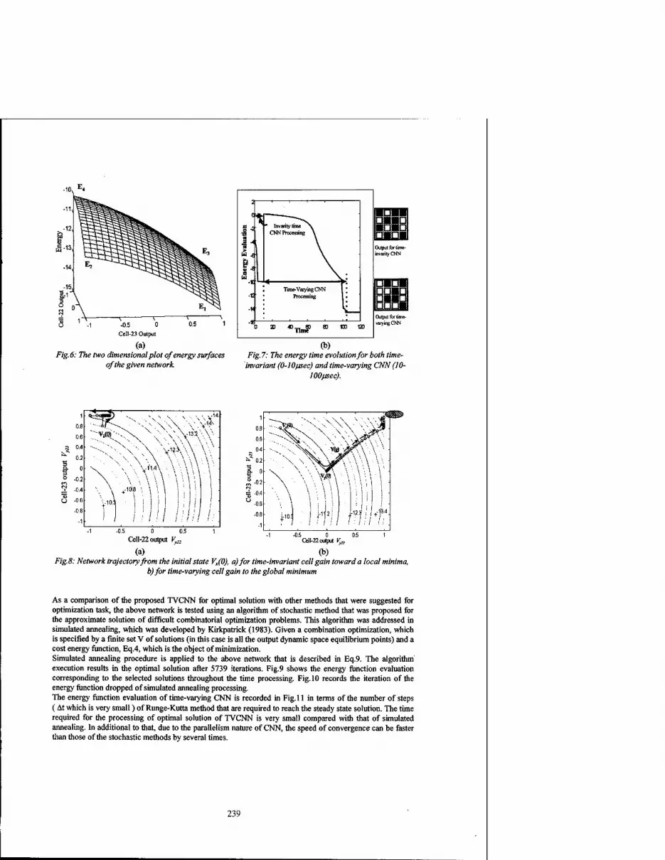
Fig. 6.

-0.5 0 0.5 1

Cell-23 Output

(a) The two dimensional plot of energy surfaces

of the given network.

t ■on S -1

* • Invarity time ^ URIN * w

CNNProcessuig \ DHtH = -< * Output for time-

H * invantyCNN

^ e

-10 ^ x,. ^^_^^_

Time-Vaiying CNN I " HnSn -t Processing 1 * HliBH ■V OODB ■1

Output for time-

) 2D O^n® 80 100 12D varying CNN

(b) F/g. 7: r/ie energy time evolution for both time-

invariant (0-10fisec) and time-varying CNN (10- WOfjsec).

■,NV\ V--WV"

"•-■■, - \ v \ ■ \ ■ \ \ \ \ •

-0.5 0 0.5

Cell-22 output Vy22

(a) Fig.8: Network trajectory from the initial state Vx(0), a) for time-invariant cell gain toward a local minima,

b)for time-varying cell gain to the global minimum

As a comparison of the proposed TVCNN for optimal solution with other methods that were suggested for optimization task, the above network is tested using an algorithm of stochastic method that was proposed for the approximate solution of difficult combinatorial optimization problems. This algorithm was addressed in simulated annealing, which was developed by Kirkpatrick (1983). Given a combination optimization, which is specified by a finite set V of solutions (in this case is all the output dynamic space equilibrium points) and a cost energy function, Eq.4, which is the object of minimization. Simulated annealing procedure is applied to the above network that is described in Eq.9. The algorithm execution results in the optimal solution after 5739 iterations. Fig.9 shows the energy function evaluation corresponding to the selected solutions throughout the time processing. Fig.10 records the iteration of the energy function dropped of simulated annealing processing. The energy function evaluation of time-varying CNN is recorded in Fig. 11 in terms of the number of steps (At which is very small) of Runge-Kutta method that are required to reach the steady state solution. The time required for the processing of optimal solution of TVCNN is very small compared with that of simulated annealing. In additional to that, due to the parallelism nature of CNN, the speed of convergence can be faster than those of the stochastic methods by several times.

239

-■4 - -

•r6

s

Ill liiLÜ IJ JL AIM II .,JHI - i \m\mminimmmmi,mi

-12 \WW Wr']r^WI^Irm' -1-3 M If" r T nIHf TJ.._.

2000 Nimbi

3000 4000 r ofltcralioBi

fig. 9: 7?ie energy function evaluation corresponding to each iteration. The circle indicates to the optimal solution

H Fig. 10: The energy function dropped iterations

corresponding to the test shown in Fig. 11 Fig.II: The TVCNN energy function evaluation

corresponding to the number of iterations

3. Conclusion In this paper, we have presented an electrical engineering method to find the global solution of quadratic

function. Problems from this category can be solved, by firstly mapping it onto cellular-neural network energy function form, and then the optimization is achieved by minimizing the energy function with the proposed TVCNN. Much future work clearly remains. Most important is the development of practical application of this method.

4. References [1] Chua L. O. and Yang L: Cellular Neural Networks: Theory" IEEE Trans. Circuits and System, vol.35, pp.

1257-1290, Oct. 1988. [2] Sheu B. J. and Choi J: "Paralleled Harware Annealing for Optimal Solution"Neural Information

Processing and VLSI, Kluwer Academic Publishers, Boston 1995. [3] Sa. H. Bang, B. J. Sheu: T. H.-Y. Wu: Optimal Solution for Cellular Neural Networks by Paralleled

Hardware Annealing" IEEE Trans, on Neural Networks, vol. 7, no 2, pp. 440-454, March 1996.. [4] Nasser N. Kamiss Al-Ani and T. Kacpszak: Computer Simulation of Time-Varying CNNs" Third

Conference Neural Networks and their Application, Kula,Poland, 14X.1997. [5] Nasser N. Kamiss Al-Ani and T. Kacprzak: Image Processing using Time-Varying Cellular Neural

Networks" fifth IEEE International CNN and their Applications, pp. 319-324 London 1998. [6] M. Gilli, P.P. Civaller, T. Roska, and L. O. Chua: Analysis of Time-Varying Cellular Neural Networks for

Quadratic Global Optimization" International Journal of Circuit Theory and Applications, 26, pp. 109- 126, 1998.

[7] S. H.aykin: Neural Networks, Maxwell Macmillan International, 1994. [8] V. M. Mladenov, D. M. W. Leenaerts, and F. H. Uhlmann: First Order Estimation of the Basin of

Attraction of Stable Equilibrium Points in CNNs" Proceeding of the ECCTD'97, pp.684-689, Budapest, Sep. 1997.

[9] Nasser N. Kamiss Al-Ani, Kacprzak T.: Basin of Attraction of Time-Varying Cellular Neural Networks for Optimization Tasks" Polyoptimization and CAD Proc. pp. 15-22, Mielno, Poland, 1998.

240

2000 6™ IEEE International Workshop on Cellular Neural Networks and Their Applications Proceedings

Evolutionary Learning Strategies for Cellular Neural Networks

R. Kunz and R. Tetzlaff

Institut für Angewandte Physik, Universität Frankfurt Robert Mayer-Straße 2-i, 60054 Frankfurt a. M., Germany

phone: +49 69 798 28317, fax: +49 69 798 28865 R.Kunz@rz.uni-frankfurt.de

ABSTRACT: In this paper a new learning algorithm for Cellular Neural Networks is presented based on evolutionary strategies. The proposed global optimization proce- dure is discussed in detail and the performance on various parameter determination problems will be shown afterwards.

1. Introduction

The universal Cellular Neural Networks (CNN) paradigm [1] has been studied in various investigations, which are leading to many different applications, e.g. image processing, by solving nonlinear partial differential equations or by modelling complex natural phenomena. Generally a CNN is an arrangement of coupled cells, where all cells interact only within a local, usually small neighborhood with its neighbors. A CNN can be described by a system of coupled nonlinear differential equations

ii = F(xi,zi,uj,yj) (1)

where the elements of the vectors üj,yj are the inputs and cell outputs yi = f(xi) of all neighbor cells Cj £ Ni(r). The set of CNN parameter values is sometimes called a CNN-gene [3]. For some applications this gene can be determined analytically for other problems a parameter training has to be performed. In recent publications [4, 5, 6] different training algorithm were introduced, some of them are limited to a special CNN type, other are endangered by local minima. In this paper we will introduce an alternative method for the determination of the CNN-gene based on an evolutionary process (ELS). [7]. In the following sections, we will first define an evolutionary process in the case of CNN, then we introduce a new learning procedure. Finally the performance of the learning procedure is evaluated for 3 different well studied problems and for a new interesting problem.

2. The evolutionary strategy

A CNN-gene consists of all CNN parameters with a certain task for a given network. In the following definitions evolutionary syntax for CNN is introduced.

Definition 1: A feature is a value or a function describing one concrete interaction between CNN cells or actions on CNN cells at a given position in the network, i.e. the feedback connection of a cell itself.

Definition 2: A CNN operation consisting of a certain number of features is called an individ- ual I = I(ai,a2,bi,b2,—,i), for example the edge detection operation is defined by Z'^ß, 1,1,1,1,1,1,1,1,1,3).

Straightforward, a population P is introduced here. Definition 3: A number N of individuals Z sharing the same structure of features are forming a population P = P{I\,X2,—1N). For example Zi(l, —1,0) and Z2(2,-3,0) are members of the same population, neither Z3(2, -3,0,1) nor Z4(-l, -1) belong to it.

0-7803-6344-2/00/$10.00 ©2000 IEEE 241

It is important to clarify that in one population only individuals having the same number of features describing the same connections are included. Of course all those individuals can and generally do have different behavior in their result. For example the and template and the or template are members of the same population but produce different results.

Definition 4: A generation G(P, k) consists of a population P at a given epoch of the evolution k; here a evolution is equal to the iteration step of the optimization procedure. For example G(P, 0) describes the initial generation and G(P, 1) its child generation. Every new generation is

' created from its parent generation with major or minor modifications.

Definition 5: A desired behavior that an individual should fulfill is called the environment. This is usually the optimization target. An individual is stated fit if it well suits its environment, measured by a so called fitness function.

3. Outline of the algorithm

To start a learning procedure, firstly a generation G(P,0) will be initiated, where all N individuals will be initialized by random numbers. Each individual has the same number M of features. To create such a population, we use different methods: normal distributed or uniform distributed random numbers ß with zero mean and a given but free to choose initial variation or a variation of an equidistant fit with a fixed distribution range where the distance of an individual to their nearest neighbours is equal for each individual.

G{P,0) D Xi = p, 0<i<N (2)

The function F(l) is used to define the fitness of each individual in the population to the given environ- ment. Here the mean square error (MSE)

^(i) = I £(</?(*)-</?«)2 (3)

or the absolute mean error (AMSE)

ni) = ^E(lwf(0-»f(t)l) (4) j=l

is considered, y* denotes the output of a cell of the Z cells in the environment. Now the selection starts by creating the next generation based on the actual one. K < M individuals of the population having the best fitness are the parents of the following generation G(P, k + 1). Here the children were obtained by a superposition of the parents features with small random numbers p, either normal or uniform distributed with zero mean.

Ii(G(P,k + l)) = lj(G{P,k)) + p, je[l,K],i£[l,M] (5)

Additionally two other aspects were taken into account to create the next generation. One describes the case of mutating or crossing some features of two childs as shown in Fig. 1. The crossing point and the effect of crossing is determined randomly. Furthermore the case of an immigration

G(k + l,P)=G{k,P) + Ik, lk<?G(k,P) (6)

is also considered, where the new individuals Ik are initialized the same as the first generation. Both aspects are necessary to avoid a fast convergence of a population to a local minimum. The new generation then consists of the parents and children, of immigrants and mutated children. The algorithm continues until either a predefined number of iterations is reached or a desired minimum is found.

242

:

s X |al a2 a3 a4 a5 a6 a7 a8| lal a2a3 ! M b5 b6 b7b8 1

to» V ^ A T |blb2b3 M b5 b6 b7 b8| | bl b2 b3; a4 a5 a6 a7a8 |

crossing point

childs

2

cro

parents

ssing point

Figure 1: The crossing of features of two parents.

3 4

Figure 2: Error surface for the and template at two different bias values of (a) I = -1 and (b) I = -1.2. a and b denote the two free parameter of this template.

4. Results

The ELS has been implemented in the universal simulation system SCNN 2000 [8] and its performance has been measured for various cases. In this paper image processing, the minimization of parameter deviations considering tolerances in hardware implementations and a modelling problem will be discussed.

4.1. Image processing

For the training of an image processing template, the well known and template [14] was considered. Its individual consists only of three features, which are J""d = (a = 1, b = 1, / = 1.5). The error surfaces for different bias values are shown in Fig. 2.

In this case, the ELS finds the correct location within k = 56 generations, with a gradient based algorithm, 600 iterations were necessary to obtain this result. The performance of the parameter training is shown in Fig. 3.

As a further example a training of the average template has been performed, leading again to a fast and accurate determination of the parameter values, the MSE is shown in Fig. 4a.

4.2. Minimizing parameter deviations

We have shown [10] that minimizing the effects of parameter variations improves the accuracy of hardware implementations significantly. Here the ELS were used to minimize such effects of deviated

243

MSE Evolutionary strategies )K Backpropagation X

-0.5

Figure S: Error surface for the and template and development of the learning process for the evolutionary process and for a standard back-propagation algorithm

0.1 F

0.001

0.01

20 40 60 80 100

iteration steps

0 20 40 60 80 100 120 140

iteration steps

Figure ^: MSE vs. no. of trainingssteps for training of the average template and (b): minimizing the effect of parameter deviations on the hlf33 template.

244

Population Parents Iteration steps Cross over MSE Polynomial 500 50 65130 0.0 0.000578704 5 500 50 54174 0.05 0.00696738 2 100 50 63917 0.6 0.137478 2 100 50 66696 0.2 0.144889 2 100 50 83443 0.5 0.148365 2 100 50 61138 0.4 0.147439 2

Table 1: Results by applying different ELS leading to approximations DcNN{k)-

templates described in [6]. Firstly the parameter of a CNN were modified with uniform distributed random numbers, leading to a translation variant CNN, showing the behavior of hardware realizations. Then the template elements will be re-adjusted with an optimization procedure in order to minimize the difference of the cell outputs to those of a simulated error free network. In previous investigations always gradient based methods have been used. The application of ELS leads in all treated cases to results with the same accuracy. One typical result for a network with 80 x 80 cells is shown in Fig. 4b. Thereby, with uniform random values, each element of the hlf33 template was modified with a standard deviation M = 10%.

4.3. Analysis of brain electrical activity in epilepsy

Different investigations [11] showed that the spatio-temporal behaviour of brain electrical activity in epilepsy can be characterized by estimates D%(k) of an effective correlation dimension in many cases. Especially, we have shown [12, 13] that the dimension DJW can De approximated by DcNN(k) with a high accuracy. DCNN(k) is a function of CNN cell output values. In this paper we have studied the performance of ELS by a determination of CNN leading to aproximations DCNNW of D%{k).

DCNN(k,m) = H({vj{tT)\i £ [1,M]}), M<M (7)

In this paper an approximation DCNN{k,m) of D%(k,m) with 0 < D£(/fc,m) < 10 is obtained by a determination of the normalized average

H = TfT,yj(tr) + h 0<H<10 (8)

of the cell outputs. Thus, by calculating DCNN(k, m) for all signal segments of a recording, a so called CNN dimension profile follows, which is compared to the result obtained with D$(k). Results for a data set of one patient are given in Table 1 and Fig. 5. Hereby the maximum variation \i of the randomly distributed individuals is set to 10, always the piecewise linear output function and Neumann boundary conditions were used. In all treated cases, a feedback template with a neighborhood radius N = 1 and a space invariant bias were determined. As Table 1 clearly shows, an increasing number of individuals within a population always yield to better results, which is caused by an improved parameter distribution in the parameter space. Up to 46 parameters were determined throughout these optimizations. Finally, the

5. Conclusion

Throughout various calculations, ELS has to be proven to be powerful learning algorithms. It enables a global search and is especially suited to problems, where local minima of the MSE occur at the cost of speed and/or memory requirements.

6. References

[1] L.O. Chuaand L. Yang: " Cellular Neural Networks: Theory and Applications"; IEEE Transactions on Circuits and Systems vol. 35, pp. 1257-1290, 1988.

245

1

0.1

0.01

0.001

0.0001

I

I I !

I I -1 L ^

'. iJ i i i— 1—:

0 10000 20000 30000 40000 50000

Iteration steps

Figure 5: MSE vs. no. of trainingsteps. Determination of a CNN for the analysis of brain electrical activity.

[2] V.Ciraagalli and M.Balsi: " Cellular Neural Networks: A Review"; Proc. 6th Italian Workshop on Parallel Architectures and Neural Networks, Vietri sul Mare, Italy,1993.

[3] L. O. Chua: CNN:" A paradigm for complexity"; World Scientific Series on Nonlinear Science, Series A, Vol. 31, 1998.

[4] J.A. Nossek: " Design and Learning with Cellular Neural Networks"; Proc. IEEE CNNA 94, Rome, pp. 137-146,1994.

[5] M. H"anggi and G.S. Moschytz: Attacking the General Classification Problem with CNNs, Proc. ECCTD99, pp. 771-774, Stresa, Italy, 1999.

[6] R.Tetzlaff, R.Kunz and D.Wolf: " Minimizing parameter deviations on Cellular Neural Networks" Proc. ECCTD 97, pp357ff, Budapest, Hungary, 1997.

[7] Charles Darwin " On the Origins of Species by Means of Natural Selection",1856

[8] R. Kunz, R. Tetzlaff and D. Wolf: " SCNN: A Universal Simulator for Cellular Neural Networks"; Proc. IEEE CNNA 96, Sevilla, pp. 255-260, 1996.

[9] F. Puffer, R. Tetzlaff and D. Wolf: " A Learning Algorithm for Solving Nonlinear Partial Differential Equations with Cellular Neural Networks (CNN)"; Proc. URSI ISSSE, San Francisco, pp 501-504, 1995.

[10] R.Tetzlaff, R.Kunz, G.Geis and D.Wolf: " Minimizing the Effects of Tolerance Faults on Hardware Realizations of Cellular Neural Networks"; Proc. CNNA 98, London, pp 254-258, 1998.

[11] K. Lehnertz and C. E. Elger: "Can epileptic seizures be predicted?" Evidence from nonlinear time series analyses of brain electrical activity, Phys. Rev. Lett, Vol. 80, pp. 5019-5022, 1998.

[12] R.Tetzlaff, R.Kunz and D.Wolf: " Analysis of Brain Electrical Activity in Epilepsy with Cellular Neural Networks (CNN)"; Proc. ECCTD 99, Stresa, Italy, 1999.

[13] R. Kunz, R. Tetzlaff and D.Wolf: " Brain electrical activity in epilepsy: Characterization of the spatio-temporal dynamics with Cellular Neural Networks based on a correlation dimension analysis"; Accepted for publication at the ISCAS 2000, Geneve.

[14] T.Roska and L.Kek: " CSL: CNN Software Library"; Version 7, Budapest, 1997.

246

2000 6™ IEEE International Workshop on Cellular Neural Networks and Their Applications Proceedings

Template Design Methods for Binary Cellular Neural Networks

Pier Paolo Civalleri and Marco Gilli Dipartimento di Elettronica, Politecnico di Torino, Torino, Italy

civalleri@polito.it; gilli@polito.it

ABSTRACT: The problem of template design for cellular neural networks (CNNs) with binary outputs is addressed. A theorem is provided, that yields some rigorous conditions for the correct behavior of a CNN and allows to develop exact and simple design rules.

1 Introduction

Cellular neural networks are analog dynamic processors, that are suitable for solving complex array signal processing problems [1, 2J. A CNN can be described as a 2 or 3-dimensional array of identical nonlinear dynamical systems (called cells), that are locally interconnected. In most cases the connections are specified through space-invariant templates (that consist of small sets of parameters identical for all the cells).

In this paper we restrict our attention to stable networks, that are exploited for processing binary images (i.e. to networks whose attractors are only stable equilibrium points, that give rise to binary outputs). This choice is supported by the fact that this class of CNNs (called binary CNNs) is exploited in most applications.

As pointed out in [3], the strategies proposed for the design of stable templates can be divided into 3 categories: (a) intuitive design, which is mainly based on extensive simulations; (b) learning and genetic algorithms; (c) direct template derivation. The first two techniques have allowed to discover several useful templates, but do not provide a deep understanding of the global dynamics of the CNN, that is the fundamental step for developing a robust design method. The direct template derivation is essentially based on the following two steps: (i) a definition of a set of local rules, that depend on the specific application: for example to impose that all the white cells (output equals to —1) surrounded by a given number of black cells (output equals to 1), become black; (ii) the determination, according to the local rules, of the sign of the initial derivative (i.e. the derivative at t = 0) of the cell states. The major drawback of this method is that, apart from uncoupled networks and some kinds of unidirectional templates [3], the knowledge of the initial derivative is not sufficient to rigorously predict the asymptotic dynamics of the network and therefore to ensure that the local rules are correctly implemented by the CNN. However, despite some disadvantages, the techniques based on the direct template derivation appear to be more suitable for CNN design, because they allow to understand the network spatio- temporal dynamics and to develop methods for robust design [4].

In this paper we firstly define rigorously the problem of the design for binary templates. Then we t enunciate a theorem that yields some conditions for developing rigorous and simple design rules, based

on the direct template derivation. This theorem extends the results presented in [5] and [6], that mainly refer to CNNs with monotonic behavior.

2 Design of binary CNNs

A CNN composed by N x M cells is described by the following normalized state equations

|j>l<r,l«l<r M<r,|(|<r

where A and B are the space-invariant templates, r denotes the neighborhood of influence of each cell, xij and uy represent the state voltage and the input voltage of the cell, whose coordinates in the

0-7803-6344-2/00/$10.00 ©2000 IEEE 247

Input image (t = 0) Output Image (t = 20)

1

2 ■■■:-•■:•-■:■■

3....:...;....:.. ■■ |..;....;....;.-

4...-;...:...-:..

6 ■■•;■• ■ ■:•■••:■■ ■ 7 ■■:■■■:■■:■■

8 ■ ■

9 ....;...;....-, .:...:. .:...;....:....;...

0 1 2 3 i 5 01 23456789 10

Figure 1: CNN with zero input, described by template (3). In the input image the white cell state voltages have been set to -1.1, whereas the black cell state voltages have been set according to the following rule: £3,6 = ^4,5 = £5,4 = ^5,6 = 1-3; 14,7 = ^6,5 = Xe,6 = ^6,7 = 1-1-

regular grid are (i,j); ytj is the output voltage, that in most applications has the following piecewise linear expression:

Hereafter we assume that the inputs uy are constant. In the following, with the term saturation region we indicate a linear region of the state space where all the output voltages ?/y are saturated. A saturation region will be denoted by a vector or a matrix, containing as entries the output voltage values.

' We assume that the CNN be stable; we also suppose that the central term A00 satisfies the inequalities Aoo > 1, thereby implying that the stable equilibrium points are located in saturation regions (i.e. such that for each cell the outputs are binary, yy = ±1).

The behavior of a stable CNN can be described as a nonlinear mapping M, that to each initial condition yy(0) £ {-1,1}N*M and each input u0- € {-l,l}JVxM assigns an output, that corresponds to the steady-state behavior of the network, i.e. yy(oo) £ {-l,l}NxM.

Under this assumption, the CNN analysis and design problems could be stated as follows:

CNN analysis: given the templates A and B, and the bias /, determine the mapping M implemented by the templates.

CNN design: given a mapping M, determine two suitable A and B templates and a bias / (if they exist) that implement the mapping.

However this formulation is not satisfactory, because there exist some cases in which, for a given input image and fixed templates, the output image is not unique. As an example of this kind of behavior, let us consider a CNN composed by 10 x 10 cells with zero input and bias terms, described by the well known average template:

~ 0 1 0 ~

A = 1 2 1

0 1 0

(3)

Let us assume that the CNN processes the input image shown in Fig. 1, where white and black pixels denote that the corresponding output voltages j/y are set to -1 and 1 respectively. The output images reported in Figs. 1-3 show that identical input images may correspond to different state voltage initial conditions and therefore give rise to different output images.

This kind of behavior is not acceptable for image processing applications, for at least two reasons: 1) the mapping M is not unique and then not well defined; 2) a small perturbation of the state voltage initial conditions, that does not alter the input image, can cause the convergence to a wrong output image.

248

Input image (t = 0) Output image (t = 20)

0 12 3 4 5

Figure 2: CNN with zero input, described by template (3). In the input image the white cell state voltages have been set to —1.1, whereas the black cell state voltages have been set to 1.1.

Input Image (t = 0) Output image (t = 0. ! ! : : ! ! r

= 20)

e........,.........^^^^m ...;...|...

7 ....;....: : ;....:.... = ....; ■■■:■■■■:■••

...: 0 12 3 4 5 0 12 3 4 5

Figure 3: CNN with zero input, described by template (3). In the input image the white cell state voltages have been set to —1.1, whereas the black cell state voltages have been set to 1.8.

Therefore it is important to identify a class of templates and of initial conditions for which the mapping M is unique.

As a preliminary step we state the following definitions:

Definition 1: A cell (i;j) lying in a saturation region such that:

Am - 1 + ^2 API yt+pJ+t Vv < ° (4) |p|<<-,|«|<r

is said to be active. A cell is said to be inactive, if it is not active.

Definition 2: A saturation region 72.2 is said to be directly reachable from a saturation region Hi, if its outputs can be obtained from those of V,\ by substituting to the inactive cells their saturation value and to the active cells either +1 or —1

Definition 3: A saturation region Hn is said to be reachable from a saturation region Hi, if there exists a sequence of saturation regions H2, ••• K»-i such that:

• V,„ is directly reachable from 7J„_i;

• for all k S [2, n — 1], TZi, is directly reachable from 7?.*_i.

Definition 4: A saturation region is said to be stable if it contains a stable equilibrium point (i.e. all the cells are inactive).

The following theorem, that for lack of space is reported without proof, yields a sufficient condition for having a well defined mapping.

249

Input image (t = 0)

0123456789 10

Output image (t = 20)

0 1 2 3 4 5 6 7

Figure 4: Image processing performed by a CNN with zero input, described by template (5).

Theorem: Let us consider a CNN described by the templates A and B, the bias / and by the input uy. Let t/y(0) be the input image corresponding to the initial saturation region H.. If the set of all the regions reachable from region 1Z contains only one stable region, then the output image yy(oo) is unique for all the state voltage initial conditions xy(0) and the mapping M is well defined.

As an example of application of the above theorem let us examine a very simple CNN, composed by only 6 cells and described by the opposite-sign templates [-0.9, 2, 0.9]. Let us assume that the input image be represented by the saturation region H = (+1 + 1 -1 - 1 + 1 + 1). It is easily verified that the second and the fourth cell are active and that the set of all the saturation regions, that are directly reachable from U is (+1 ±1 - 1 ±1 +1 +1). Finally it is derived that the set of all the saturation regions that are reachable from 11 can be expressed as: (+1 ±1 -1 ±1 +1 +1)U(+1 -1 +1 +1 +1 +1) and that this set contains only one stable region, i.e (+1 -1 +1 +1 +1 +1), that represents the actual output image, observed through the simulation.

The theorem that we have presented may be exploited for both CNN analysis and design. As far as the analysis is concerned, the theorem allows to establish: 1) if for given templates, bias term and input image, the output image is unique for all the state voltage initial conditions; 2) the set of the input images for which a CNN behaves correctly (i.e as expected by the template designer).

In order to clarify point 1, it is possible to compute the stable saturation regions that are reachable from the input image of Fig. 1, for the CNN described by template (3): it turns out that these regions are 13. We have verified that, by suitable choosing the initial conditions, the CNN may actually converge to 13 different output images for the same input image: Figs. 1-3 show only three of the possible outputs.

As mentioned in point 2 above, a more useful utilization of the theorem is the determination of the input images for which the CNN works properly. To this purpose, let us consider the network described by the template called smkiller, that is useful for deleting small objects and is described in [3]:

A =

1 1 1

1 2 1

1 1 1 (5)

This template should work according to the following two simple rules: a) all the black cells having more than four white neighbors become white; b) all the white cells having more than four black neighbors become black.

Let us assume that the CNN processes the input image shown in Fig. 4. It is readily shown that the only stable reachable region is that with all outputs j/y equal to -1: therefore, as shown in Fig. 4, the theorem easily predicts that in this case the CNN does not behave correctly (i.e in agreement with the design rules a) and b) reported above).

As a final example, let us consider the input image shown in Fig. 5. In such a case the only stable reachable saturation region is the output image reported in Fig. 5, i.e. the theorem is able to predict that the CNN works properly.

From the above considerations it turns out that the theorem above can be exploited also for CNN design. The procedure that we suggest can be synthesized by the following two major points: I)

250

Input Image (t = 0) Output Image (t = 20)

0 12 3 4 5 6 7 0123456789 10

Figure 5: Image processing performed by a CNN with zero input, described by template (5).

determine the templates, by imposing the sign of the state initial derivative (i.e the number of active cells), according to suitable local rules, as described in [3] and [4]; II) check the correctness of the templates, for the actual input images, by applying the theorem.

It is worth noting that the monotonic templates studied in [5] and [6] are a particular case of the templates satisfying the assumptions of the above theorem, for each initial condition.

3 Conclusion

We have studied the design problem for binary CNNs (i.e stable CNNs with binary outputs), that are exploited in several applications.

We have provided a theorem that yields a sufficient condition for the correct behavior of these networks and we have shown the usefulness of the theorem through some examples.

Then we have suggested a possible design procedure, based on the determination of the templates, by imposing the sign of the state initial derivative, and on the check of the correctness of the template through the proposed theorem.

References

[1] L.O.Chua, T. Roska, "The CNN paradigm," IEEE Transactions on Circuits and Systems: I, vol. 40, no. 3, pp. 147-156, March 1993.

[2] Special issue on spatio-temporal signal processing with analog CNN visual microprocessor, Journal of VLSI Signal Processing systems, Kluwer Ac. Publisher, November-December 1999.

[3] A. Zarandy, "The art of CNN template design," International Journal of Circuit Theory and Ap- plications, vol. 27, no. 1, pp. 5-23, January-February 1999.

[4] M. Hanggi, G. S. Moschytz, "An exact and direct analytical method for the design of optimally robust CNN templates," IEEE Transactions on Circuits and Systems, Part I, vol. 46, no. 2, pp. , February 1999.

[5] I. Fajfar, F. Bratkovic, T. Tuma, and J. Puhan, "A rigorous design method for binary cellular neural networks," International Journal of Circuit Theory and Applications, vol. 26, no. '4, pp. 365-373, July-August 1998.

[6] M. Gilli, "Template design methodologies and tools," Design automation day on cellular visual microprocessor (ECCTD'99), pp. 113-125, August 1999, Stresa, Italy.

[7] T. Roska, L. Kek, L. Nemes, and A. Zarandy, "CNN software library: templates and algorithms," Comp. and Auto. Ins. of the Hung. Acad. of Sei. DNS 1-1997, Budapest, 1997.

251

2000 6™ IEEE International Workshop on Cellular Neural Networks and Their Applications Proceedings

Phase Synchronization Phenomena in Generalized CNN Composed of Chaotic Cells *

A. Dabrowski, Z. Galias, MJ. Ogorzalek

Department of Electrical Engineering, University of Mining and Metallurgy, al. Mickiewicza 30, 30-059 Krakow, Poland,

e-mail: maciej@zet.agh.edu.pl

ABSTRACT: Using numerical experiments we show that the phase synchronization concept enables better insight into the synchronization phenomena encountered in a ladder type CNN structure composed of chaotic cells. In some cases when the phase plot inspection does not allow to confirm synchrony such kind of behavior can be distinguished by inspection of the phase calculated using the analytic signal approach.

1. Introduction

In nature structures composed of individual simple subsystems are wide-spread. Specific examples come from biology and medicine (tissues of living organisms) physics and chemistry (matter composed of atoms), etc. Prop- erties of such systems depend on properties of individual subsystems and the way they are coupled together. Various models describing behavior of interconnections of a large number of simple systems have been proposed by scientists. Among them lattice models, exhibiting various types of collective behavior play an important role [1, 5, 6, 11]. Among various types of collective dynamics one can observe many types of spatial, temporal or spatio-temporal ordered structures referred to as self-organization [5] or "pattern formation". "Organized" behav- ior is usually linked with coherent (synchronized) behavior of a number of subsystems in the network. Organized spatio-temporal behavior includes propagation of waves including solitons and autowaves, target waves, spiral waves and traveling wavefronts [12].

In our previous works we studied cooperative behavior in one- and two-dimensional CNNs composed of chaotic cells with resistive couplings [3, 8]. In the present study we investigate synchronization phenomena observed in a steady-state in a ring (one-dimensional CNN array with connected ends) in which each cell is Chua's chaotic circuit. In experiments we use so-called balanced cells in which a self-coupling term has been introduced in each cell enabling simultaneous development of synchronized chaotic motion in all cells. Using computer experiments we have confirmed the existence of phase synchronization.

2. Phase Synchronization

When considering coupled dynamical systems one of the most frequently described phenomena is synchroniza- tion. There are several concepts of synchronization introduced in the literature starting from synchronization of periodic oscillators (such as clocks), through synchronization with external input (periodic) signal to synchro- nization of chaotic modes. Depending on how the synchrony occurs in the systems concepts of weak, complete, generalized and several other types of synchronization have been introduced. In this paper we will consider so-called phase synchronization of chaotic oscillators. To be able to talk about phase synchronization several approaches have been proposed to describe the phase and frequency lockings in chaotic systems [9].

2.1 Determination of phase using the analytic signal concept

Using the method of analytic signal we show that for specific choices of coupling parameters the interaction of chaotic oscillators can lead to a perfect locking of their phases while their amplitudes remain chaotic and decorrelated.

*Supported by the research grant 11.120.182 from the University of Mining and Metallurgy, Krakow.

0-7803-6344-2/00/$10.00 ©2000 IEEE 253

Let us introduce first the basic notions of amplitude and phase of an arbitrary signal s (t). A general approach has been introduced by Gabor and is based on the analytic signal concept. The analytic signal tp(t) is a complex function of time defined as:

rl>(t) = s(t) + js(t) = A(tV'*(<> (1)

where the function s(t) is the Hilbert transform of s(t):

s(t) = -PV r°°^dr (2)

(where PV means that the integral is taken in the sense of the Cauchy principal value). The instantaneous ampli- tude A(t) and instantaneous phase <j>(t) of signal s(t) are thus uniquely defined.

From (2) s(t) may be considered as the convolution of the functions s(t) and l/irt. Hence the Fourier trans- form S(jw) of s(t) is the product of Fourier transforms of s(t) and l/irt. For physically relevant frequencies w > 0, S(JIAJ) = -jS(jw) i.e. ideally s(t) may be obtained from s(t) by a filter whose amplitude response is unity, and whose phase response is a constant 7r/2 delay at all frequencies.

For chaotic oscillators we can calculate the phase from any observable variable s(t) so there is no unique phase of chaotic oscillations. However in some cases observables provide phases which agree with intuitive definition. To study phase synchronization of coupled chaotic oscillators we calculate phases of each of the oscillators and check the weak locking condition |n0, - m<fc| < canst, (usually we require the constant to be small). In this paper we will just consider the case m = n = 1. In the data taken in some physical observations such as electrocardiograms and pulmonary rhythms such fractional phase synchronization phenomena have been confirmed.

Notes: 1. One should be careful during the computation of phases especially in the cases when the signal changes sign of the slope near the origin - in such cases we often observe in calculation phase jumps of 2ir. 2. Determination of chaotic signal phase and phase synchronization is highly dependent on the choice of the coordinate system - even a constant bias added to the measured signal can change the results completely.

3. Experimental Setup

Let us consider a one-dimensional CNN composed of generalized cells namely simple third-order electronic oscillators (Chua's circuits). The oscillators are coupled bi-directionally by means of two resistors cross-connected between the capacitors C\ and C2 of the neighboring cells. Every cell is connected with two nearest neighbors. The first and the last cells are also connected thus forming a ring of cells. The dynamics of the l-D CNN array composed of n cells can be described by the following set of ordinary differential equations:

C2ii = -Vi + (G- 2G1)(zi - Xi) + +Gi(2,_i - Xi) + Gi («,-+i - xt),

I4)i = xit (3) CiZj = (G - 2GI)(ZJ - Zi) - f(zi) + +Gi(ii_i - Zi) + G1(i,-+1 - z{),

where i = 1,2,... ,n and we use the following boundary conditions x0 := xn, zo ■= z„, i„+i := xi and zn+i := z\ and / is a five-segment piecewise linear function:

/(*) = m2z + -(mi- m2)(|z + flw| - |z - Bp,|)

\(m0-m,){\z + Bpl\-\z-BPl\). (4)

As in our previous studies we use typical parameter values for which an isolated Chua's circuit generates chaotic oscillations — the "double scroll" attractor:

Ci = 1/9F, C2 = IF, L = 1/7H, G = 0.7S, m0 = -0.8, mx = -0.5, (5) m2 = 0.8, B„, = 1, BP2 = 2.

254

PH» 0 m 0 a 0 11 0 m 0 #r 0

•

300 300 300 300 300 300

200 ZOO 200 200 200 200

100 100 100 100 100 100

tOOO 2000 0 1000 2000 1000 2000 0 1000 2000 0 1000 2000

10 10 . 10

-K "W*>- W^W*1

«^rr-vr^

1000 2000 0 1000 2000 0 1000 2000 0 2000 0 10OO 2000 0

Case 1 - G\ = 0.001 - lack of synchronization in the case of very weak coupling between the cells.

Figure 1: First row - projection of extractors in each of the cells; Second row - Xi+i variable plotted against the Xi (in the previous cell; Third row - phase calculated using the Hüben transform plotted against the iteration number; Last row - phase difference between the current and previous cell.

4. Simulation Results

Let us consider the CNN composed of n = 7 circuits connected in a ring structure. In the experiments we have considered the uniform coupling and the coupling resistance is a variable parameter.

One can observe very interesting phenomena of synchronization when the coupling coefficients are appro- priately adjusted. In the successive figures we have shown respectively in rows (a) the phase plots showing projections of attractors; in rows (b) xi variables of two successive cells plotted against each-other; in rows (c) the dependence of the phase (defined by the Hilbert transform) of the signal xi from a given cell on the iteration number; (d) the difference of the phases of two successive cells.

Fig.l shows results of experiments when the coupling between cells is very small (Case l.-G — 0.001). All the cells are almost independent and behave chaotically displaying a double scroll attractor. The plots showing dependence of variables of successive cells do not indicate any type of synchronization.

When the coupling coefficients are larger (Cases 2 - 4 in Fig. 2 and 3) due to interaction between the cells in the steady-state the network behaves chaotically, with some cells developing Roessler-type attractors in the upper and some in the lower half-space (compare Fig. 2). Such a state of the network will be called a pattern. With each patterns we can associate the sequence of O's and 1 's in such a way that if the ith cell operates in the upper (lower) half-space then we set the ith element of the sequence to 1 (0) [3,4].

In the cases when two successive cells synchronize in the (b) plots one can see an almost perfect bisectrice line while in the (d) row one can see a "0" phase difference line. Interesting insight into systems behavior is obtained in the cases when there is no perfect synchronization i.e. there is no more perfect line in the figures in (b) row. In some of such cases the inspection of the phases enables us to find almost perfect phase synchronization even though the phase plots does not indicate this. The phases grow with time (iteration number) but their difference remains bounded. In such cases we claim that there is phase synchronization but not amplitude synchronization (amplitudes vary chaotically).

255

0.5 -0.S 0 0.5 -0.5 0 0.5 -0.S 05 -0.5 0 0 5-0.5 0 0.5

/ / / / / / -0.5 0 0.5 -0.5 0.5 -0.S 0 0.5 -0 5 0.5 -0 5 0 0.5

300 300 300 300 300 300

200 200 200 200 200 200

100 100 100 100 100 100

1000 2000 0 1000 2000 0 10OO 2000 0 1000 2000 2000 0 1000 2000 0 1000 2000

#v**v M:«ui •mr-itfw mS** 1000 2000 0 1000 2000 0 1000 2000 0 1OO0 2000 0 2000 0 1000 2000 0 IOO0 2000

Case2-Gi = 0.17-first and second cells are perfectly synchronized. For some other cells inspection shows existence of phase synchronization

The amplitudes very chaotically - the phase difference is bounded.

■j -y ■fc*^ ■/ -? -7 -I ^^0r

-0.5 0 0.5 -0.5 0.5 -0 5 0 0.5 -0 5

////// -0.5 0 05 -as OS -0.5 0 05-0 5 0 OS -0.5 0.5 -0 5 0 0.5 -0.5 0 0.5

«<H>

300 300 300 300 300 300

200 200 200 200 200 200

100 100 100 100 100 100

0 1000 2000 0 2000 0 1000 2000 0 1000 2000 2000 0 1000 2000 0 1000 2000

— 50 ^ 0 50

0 0 -50

-60

1000 2000 0 1000 2000 0 1OO0 2000 0 1000 1000 2OO0 0 10O0 2000 0 1000 2000

Case 3 - G\ = 0.1979 - first and second cells are perfectly synchronized Cells 2 and 3 and 7 and 1 are phase-synchronized.

Other cells are not synchronized phase difference changes in a monotone way.

Figure 2: First row - projection ofattractors in each of the cells; Second row - x1+i variable plotted against the xt (in the previous cell; Third row - phase calculated using the Hilbert transform plotted against the iteration number; Last row - phase difference between the current and previous cell.

256

m ?.

10 2

10 2

10 2

0 2

1

10 2

10 0.5 -0.S 0 0.5 -0.5

/ / / / 0.5 -0.S 0 0.5 -05 0 0.5 -0.5

400

300 300 300 300 300 300

200 200 200 200 200 200

100 100 ^^ 100 100 100

0 ^^ 100

n 1000 2000 0 IO00 2000 1000 2000 0 tOOO 2O00

0 H^mifcuW'.' Hiy fiifim

1000 2000 1000 2000 0 1000 2000 0 1000 2000 1000 20O0

Case 4 - Gi = 0.306 - coexisting phase synchronized and desynchronized states.

Figure 3: First row - projection ofattractors in each of the cells; Second row - xi+i variable plotted against the Xi (in the previous cell; Third row - phase calculated using the Hüben transform plotted against the iteration number; Last row - phase difference between the current and previous cell.

In the Fig. 2, and 3 one can see some results obtained for different coupling parameter values. One can observe various types of synchronization - from lack of synchronization to perfect synchronization of some cells, phase synchronization of subsets of cells and lack of phase synchrony. It is interesting to notice the coexistence of various synchronized and non-synchronized states. In the plots the phase differences are plotted against time (iteration number) - if the phase difference remains bounded within a small interval we consider such two cells phase synchronized. Cells are perfectly phase synchronized if the difference is constant in time. I many cases large variations of phase are visible. In the figures one can distinguish also some cases when the phase difference varies in a monotone way. In these cases possibly there could exist more complex types of synchronization (not one-to-one).

It is interesting to compare results of computations carried out in the Cases 2 and 3 as shown in Fig. 2. Comparison of the respective three first rows seems to indicate that the behavior in both cases is almost identical (shape and position of attractors in the phase plots, phase plots of variables in successive cells). Only inspection of the last row in each case reveals the true differences in synchronization!

For the sake of simplicity we looked into the synchronization of successive cells only and we considered here the phase differences between the chaoticaly varying voltages across the corresponding capacitors in neighboring cells. Other types of synchronizations are often visible when considering more distant cells (one could analyze eg. the k - th and ( - th cells, \k - l\ > 1).

5. Conclusions

Introduction of the notion of the phase for chaotic oscillations allows more detailed inspection and description of synchronization phenomena in generalized CNNs. In some cases when the plot inspection fails in detecting synchrony (the graph of the dependence of state variables in successive cells does not belong to or lie in a close vicinity of the bisectrice of the first or third quadrangle), calculation of phase difference enables determination of more generalized synchronization phenomena. One should be however very careful with interpretation of the results as in many cases determination of phases

257

might be ambiguous - this is often the case when considering the Rössler type spiral attractors for which the measured variables do not change sign during very long time intervals.

Studies show also that not only neighboring cells might synchronize-we have also observed synchronization of sub-circuits lying far apart in the ring.

Also more complex synchronizations (m, n ^ 1) can exist - we suspect that this is the case eg. in all our tested circuits when the phase difference plots represent almost straight lines.

References

[1] V.S. Aframovich, V.l. Nekorkin, GA. Osipov, & V.D. Shalfeev:"Stability, Structures and Chaos in Nonlinear Synchronization Arrays". Eds. A.V.Gaponov- Grekhov, M.I.Rabinovich, IAP, USSR Acad.Sc, 1989 (in Russian).

[2] A. Dabrowski, Z. Galias, M.J. Ogorzalek: "Observations of Phase Synchronization Phenomena in One- dimensional Arrays of Coupled Chaotic Electronic Circuits ", Theme Issue IJBC - J. Kurths Ed. (in press)

[3] Z. Galias, M.J. Ogorzalek: "Coexistence of attractors in a one-dimensional CNN array", Proc. CNNA-98, London, pp.118-123, 1998.

[4] Z. Galias, M.J. Ogorzalek: "Study of Synchronized Motions in a One-Dimensional Array of Coupled Chaot- ic Circuits", Int. J. Bifurcation and Chaos, vol .9, No. 11, pp.2219-2224,1999

[5] H. Haken: "Synergetics; From Pattern Formation to Pattern Analysis and Pattern Recognition" Int. J. Bif. Chaos, 4, pp.1069-1083,1994.

[6] K. Kaneko: "Pattern dynamics in spatio-temporal chaos". PhysicaD 34, pp. 1-41, 1989.

[7] K. Kaneko: "Clustering, coding, switching, hierarchical ordering and control in a network of chaotic ele- ments". PhysicaD41, pp. 137-172,1990.

[8] M.J. Ogorzalek, Z. Galias, A. Dabrowski, & W.R. Dabrowski: "Wave propagation, pattern formation and memory effects in large arrays of interconnected chaotic circuits", Int. J. Bif Chaos, vol.6, No.10, pp.1859- 1871,1996.

[9] M.G. Rosenblum, A.S. Pikovsky, & J. Kurths: "Phase Synchronization of Chaotic Oscillators", Phys. Rev. Letters, vol.76, No.ll, pp.1804-1807,1996.

[10] M.G. Rosenblum, A.S. Pikovsky, & J. Kurths: "Phase Synchronization in Driven and Coupled Chaotic Oscillators", IEEE Trans. Circuits Systems, vol.CAS-44, No. 10, pp.874-881,1997.

[11] Y. Yao, & W. Freeman: "Model of Biological Pattern Recognition with Spatially Chaotic Dynamics", Neural Networks, vol.3, pp. 153-170, 1990.

[12] Theme Issue on Discretely Coupled Dynamical Systems Int. J. Bif. Chaos, vol.6, No.9-10, 1996.

258

2000 6™ IEEE International Workshop on Cellular Neural Networks and Their Applications Proceedings

CNN model for hyperbolic equations with hysteresis

Angela Slavova * Institute of Mathematics, Bulgarian Academy of Sciences

Sofia 1113, Bulgaria e-mail: slavova@math. bas.bg

Abstract. In this paper semilinear hyperbolic equation with hysteresis operator is considered. CNN model for such equation is made. Dynamic behavior of the CNN model is studied using desc- ribing function method. Traveling wave solutions are proved for the CNN model.

1 Introduction

Many dynamical systems exibit hysteresis as one of their features. In classical continuum mechanics, hysteresis behavior is inherent in many constitutive laws. If the hysteresis behavior is described using a hysteresis operator, then the mathematical model for the dynamical system consists of a system of differential equations coupled with one or several hysteresis operators, which is complemented by initial and boundary conditions.

Hysteresis constitutive laws in continuum mechanics formulated in terms of hysteresis operators lead in a natural way to partial differential equations coupled with hysteresis operators, where the former represent the balance laws for mass, momentum and inter- nal energy. From a mathematical viewpoint particularly interesting are those situations where the hysteresis operator appears in the principal part of the partial differential e- quation, since then the proofs of even basic existence and uniqueness results are linked in a non-obvious manner to certain properties of the hysteresis diagrams and of the memory structure.

The main aim of this paper is to study a class of first order semilinear hyperbolic equations, in which a memory operator occurs in the sourse term [10]:

^ + ^ + T(u) = 0, mQ=)a,b[x}0,T[. (1)

We will search for traveling wave solutions of such model which leads to study of ordinary differential equations with hysteresis. In this connection we will construct CNN model of (1) and we will study its dynamical behavior using describing function method. Finally we will make comparison between obtained results for our CNN model and the classical mathematical results for (1).

'This paper is partially supported by Grant MM-706.

0-7803-6344-2/00/$10.00 ©2000 IEEE 259

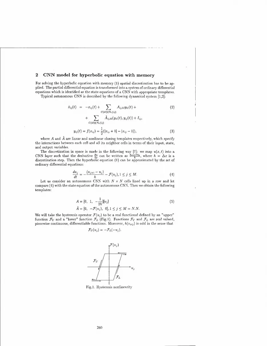
2 CNN model for hyperbolic equation with memory

For solving the hyperbolic equation with memory (1) spatial discretization has to be ap- plied. The partial differential equation is transformed into a system of ordinary differential equations which is identified as the state equations of a CNN with appropriate templates.

Typical autonomous CNN is described by the following dynamical system [1,2]:

iij{t) = -i,-j(0+ Y^ AijMyki{t) +

+ £ c(ki)eNr(i,)

Äij,ki(yki(t),yij(t)) + iij,

y«(0 = /(*«) = gfl1'-; + i| - l*o--i|

(2)

(3)

where A and A are linear and nonlinear cloning templates respectively, which specify the interactions between each cell and all its neighbor cells in terms of their input, state, and output variables.

The discretization in space is made in the following way [7]: we map u(x,t) into a CNN layer such that the derivative fs can be written as ";+■- h = Ax x h '

discretization step. Then the hyperbolic equation (1) can be approximated by the set of ordinary differential equations:

IT ui+i ■^K-),l <3<M. (4)

Let us consider an autonomous CNN with Ar x A' cells lined up in a row and let compare (4) with the state equation of the autonomous CNN. Then we obtain the following templates:

1 A = [0, 1, —\lxtj] (5)

Ä = [0, -F(UJ), 0], 1 < j < M = Ar.Ar.

We will take the hysteresis operator ^(UJ) to be a real functional defined by an "upper" function Tu and a "lower" function Ti (Fig.l). Functions Tu and Ti are real valued, piecewise continuous, differentiable functions. Moreover, /i(i'r;j) >s °dd in the sense that

Tu(uj) = -TL(-UJ).

Fig.l. Hysteresis nonlinearity

260

For the output function / of our model we will take the standard sigmoid function (3). We will take periodic boundary conditions:

«o = «M, (6)

«M+i = «1,

which make the array circular [3].

3 Dynamic behavior of our CNN model

3.1 Existence of the periodic solutions of CNN model for hyperbolic equation

(1) u3

Let us take for simplicity the following hysteresis functional J-{UJ) = -£ — Uj [8]. Then our CNN model can be written in the following form:

du; (M,+I — Uj) .«? . „ „ . _ ,, ,, ,r ._. -jf = - h -(j-uj)^<3<M = N-N (7)

or j auj M.J-I Uj ,

■nt = u*—h-+i+nM> (8)

where the nonlinearity is n(uj) = —f. In this paper we investigate the dynamic behavior of a CNN model (7) by use of

Harmonic Balance Method well known in control theory and in the study of electronic oscillators [5] as describing function method. The method is based on the fact that all cells in CNN are identical [1,2], and therefore by introducing a suitable double transform, the network can be reduced to a scalar Lur'e scheme [3,5].

We shall use the following double Fourier transform F(s,z) of functions /*,(£) [4]:

K=CO /»CO

F{s,z)= Y, z~k I fk{t)exp{-st)dt. (9) Jt=-oo J-<x>

Applying the above transform to the CNN model (7) we obtain:

sU(s, z) = U(s, z) + i[/(s, z) - ^-U(s, z) + N(U(s, z)), (10)

where the nonlinearity N(U(s, z)) is the transform of the n(uj). Then from (10) it is easy to express the state U(s,z) as a function of this nonlinearity:

"('•') = A + ,-fc-l"W«,«))- (11)

In the double Fourier transform (9) we suppose that s = iu>o and z = exp(itio), where u>o is a temporal frequency, fJo is a spatial frequency.

According to [5], H(s, z) = 3h+zh_h_1 is the transform function, which can be presented

in terms of u)0 and ti0, i.e. H(s,z) = Ha^^o):

261

where U is the state, and V is the output according to the corresponding Lur'e diagram [3]. We are looking now for possible periodic solutions of the system (7) of the form.

£4i„(w0) = Umosin(u0t+j%). (13)

Then we can approximate the output in the same way:

Vh0(w0) = Vmosin(u0t + jfl0)-

According to the describing function method we take the first harmonics, i.e. j> = 0 =$-

UnoM = Umosinu>0t, (14)

Vh0(u)0) = Vmasinu>0t, (15)

and we can find the amplitude Vma of the output:

Vm„ = - I N{Umasin4,)simpd^ = --=*. (16) * J-rr 4

Thus from (12), (14) and (15) we get

On the other side if we substitute s = ioJo and z = exp(ifto) in (12) we obtain:

ftioM = i—r n ± ■ o fc—f (18) inojo + cos S!0 + 25?n Ho — ft — 1

According to (16),(17) and (18) the following constraints hold:

„ ,„ , N-, _ h(cosflo-l-h) Umo _ _4_ Re(Ha^0)) - {cogno_l_hy + {hwo + ainno)2 ~ Vmo - f/2o (ly)

, ,rj , ^ -h(hu0 + sin %) v (cosilo - 1 - n) + (/J^O + smSJo)

Suppose that our CNN model (7) is a finite circular array of M cells. For this case we have finite set of frequences:

n„ = ^, 0<fc<M-l. (20)

Now according to the describing function method [5], if for a given value of fi0 from (20) we can find a>o and Umo from (19), then we can predict the existence of periodic solution of our CNN model for the hypebolic equation (1). From (19) after some calculations we

obtain: w0 = -^, Umo = 2^±^f^. Therefore, we have:

Proposition 1 CNN model (7), with circular array of M = N.N cells and periodic boundary conditions

u0{t) = UM(0>

«M+i = «i(')>

has periodic solution with period T0 = 2ir/u]0 and amplitude Um„ for all Q0 = jif, 0 < k< M - 1.

262

3.2 Stability of the periodic solutions of our CNN model

Describing function method predicts what the steady state solution of CNN will be-an equilibrium point, a periodic solution or non-periodic solution. We have predicted above, that in our CNN model exists periodic steady state solution. Moreover, it is possible to use this method not only to get an indication about the existence of the limit cycles, but also about their stability. Using the graphical criterion [3,5] we can give the analytical condition for the stability of periodic solutions which is:

Proposition 2 For a real valued describing function, the periodic solution is predicted to be stable if:

dIm{Ha(co)} d(l/D(Umo))_ < 0

doj ' dU, mo

From (19) after some calculations it follows that ^ < 0, and for 8(1/^m°)) = jß-

which is positive since the amplitude Uma is positive. Therefore (21) is satisfied and the predicted periodic solutions of our CNN model (7) are stable. Therefore, the following theorem is valid:

Theorem 1 Circular CNN model (7) of the hyperbolic equation with hysteresis (1) has periodic solutions with period To = 2TT/U}Q and amplitude Umo for all Ho = ^-, 0 < k < M — 1 for all M. Moreover, these periodic solutions are stable.

Remark 1. According to the Poincare-Bendixon theorem [9] applied to our case, only a set of initial conditions of measure zero will reach a periodic solution, all other trajectories will converge to an equilibrium point.

Remark 2. (Regulazing effect of hysteresis). Theorem 1 shows that the presence of hysteresis has a regulazing effect in nonlinear

wave propagation, in essential contrast to the possible occurance of discontinuous solutions in the form of shock waves that can develop for the nonlinear wave equation, that is, in the case of nonlinear superposition operator.

4 Comparison with the classical results

As we said in the begining we will search for traveling wave solution of (1). We look for a solution in the form: u(x,t) = u(x + ct), where c is the speed of the wave. It is known [11] that for a traveling wave front represented by u(x, t) is said to be a wave front if

u{x,i) -» fci as t —> — oo,u(x,t) —¥ k^ as t —> oo,

for some constants fci and k2- According to the obtained results, there exist stable periodic solutions of our CNN

model (7), such that limt^^^u^t) = const., 1 < j < M. Therefore we have proved existence of traveling wave solutions with period To = 2X/UJO and the wave front Umo.

Analogous results are proved in [10]. In other words it is proved that for T -piecewise continuous and monotone hysteresis operator, there exists a solution of (1) in the form of a traveling wave: u(x,t) = u(x.u + ct), \u\ = 1, c > 0 and such that lim^^u^) = «*, u* is a given real number, £ := x.v + ct.

263

References

[1] Chua L.O., Yang L., Cellular neural networks: Theory, IEEE Trans. Circuit Syst., vol. 35, pp. 1257-1271, Oct. 1988.

[2] Chua L.O., Yang L., Cellular neural networks: Applications, IEEE Trans. Circuit Syst., vol. 35, pp. 1272-1290, Oct. 1988.

[3] Crounse K.R., Chua L.O., Thitan P., Setti G., Characterization and dynamics of pattern formation in CNNs, Int. J. of Bifurcation and Chaos, vol. 6, N 9, pp. 1703- 1723, 1996.

[4] Gilli M., Civalleri P.P., A spectral approach to the study of propagation phenomena in CNNs, Int. Journal of Circuit Theory and Applications, 24 (1), pp. 37-47, 1996.

[5] Mees A.I., Dynamics of Feedback Systems, John Wiley, 1981.

[6] Perez-Munuzuri V. et. al., Nonlinear waves, patterns and spatio-temporal chaos in CNNs, Phil.Trans.R.Soc.Lond.A, vol. 353, pp. 101-113, 1995.

[7] Roska T., Chua L., Wolf D., Kozek T., Tetzlaff R., Puffer F., Simulating nonlinear waves and PDEs via CNN - Part I: Basic Techniques, Part II: Typical Examples, IEEE Trans. Circuit and Syst. - I, vol. 42, N 10, pp.809-820, 1995.

[8] Slavova A., Dynamic properties of Cellular Neural Networks with nonlinear output function, IEEE Trans. CAS-I, vol.45, N5, pp. 587-591, 1998.

[9] Vidyasagar M., Nonlinear System Analysis, Englewood Cliffs, NJ: Prentice Hall, 1978.

[10] Visintin A., Differential Models of Hysteresis, Appl. Math. Sei. Ill, Springer, 1994.

[11] Whitham G.B., Linear and Nonlinear Waves, John Wiley, 1974.

264

2000 6™ IEEE International Workshop on Cellular Neural Networks and Their Applications Proceedings

State-of-the-Art and Prospections for VLSI Mixed-Signal Implementations

A. Rodrlguez-Vdzquez

Institute de Microelectrönica de Sevilla Centro Nacional de Microelectrönica

Avda. Reina Mercedes s/n, 41012 Seville, Spain email: angel@cnm.us.es

Phone #:+34 5 423 99 23 Fax #: +34 5 423 18 32

0-7803-6344-2/00/$10.00 ©2000 IEEE 265

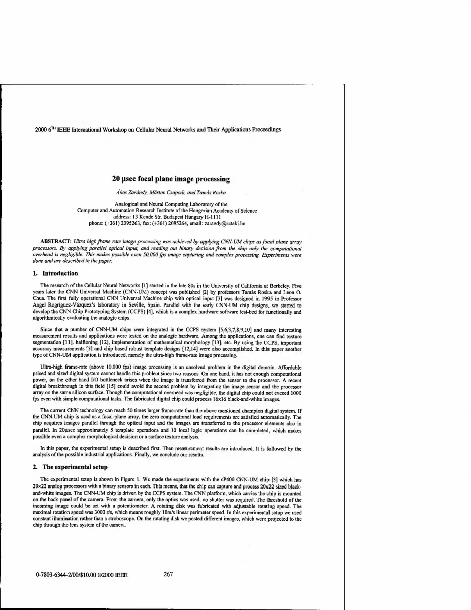
2000 6™ IEEE International Workshop on Cellular Neural Networks and Their Applications Proceedings

20 [lsec focal plane image processing

Akos Zarändy, Märton Csapodi, and Tamäs Roska

Analogical and Neural Computing Laboratory of the Computer and Automation Research Institute of the Hungarian Academy of Science

address: 13 Kende Str. Budapest Hungary H-1111 phone: (+361) 2095263, fax: (+361) 2095264, email: zarandy@sztaki.hu

ABSTRACT: Ultra high frame rate image processing was achieved by applying CNN-UM chips as focal plane array processors. By applying parallel optical input, and reading out binary decision from the chip only the computational overhead is negligible. This makes possible even 50,000 fps image capturing and complex processing. Experiments were done and are described in the paper.

1. Introduction

The research of the Cellular Neural Networks [1] started in the late 80s in the University of California at Berkeley. Five years later the CNN Universal Machine (CNN-UM) concept was published [2] by professors Tamäs Roska and Leon O. Chua. The first fully operational CNN Universal Machine chip with optical input [3] was designed in 1995 in Professor Angel Rogrfguez-Väzquez's laboratory in Seville, Spain. Parallel with the early CNN-UM chip designs, we started to develop the CNN Chip Prototyping System (CCPS) [4], which is a complex hardware software test-bed for functionally and algorithmically evaluating the analogic chips.

Since that a number of CNN-UM chips were integrated in the CCPS system [5,6,3,7,8,9,10] and many interesting measurement results and applications were tested on the analogic hardware. Among the applications, one can find texture segmentation [11], halftoning [12], implementation of mathematical morphology [13], etc. By using the CCPS, important accuracy measurements [3] and chip based robust template designs [12,14] were also accomplished. In this paper another type of CNN-UM application is introduced, namely the ultra-high frame-rate image processing.

Ultra-high frame-rate (above 10.000 fps) image processing is an unsolved problem in the digital domain. Affordable priced and sized digital system cannot handle this problem since two reasons. On one hand, it has not enough computational power, on the other hand I/O bottleneck arises when the image is transferred from the sensor to the processor. A recent digital breakthrough in this field [15] could avoid the second problem by integrating the image sensor and the processor array on the same silicon surface. Though the computational overhead was negligible, the digital chip could not exceed 1000 fps even with simple computational tasks. The fabricated digital chip could process 16x16 black-and-white images.

The current CNN technology can reach 50 times larger frame-rate than the above mentioned champion digital system. If the CNN-UM chip is used as a focal-plane array, the zero computational load requirements are satisfied automatically. The chip acquires images parallel through the optical input and the images are transferred to the processor elements also in parallel. In 20usec approximately 5 template operations and 10 local logic operations can be completed, which makes possible even a complex morphological decision or a surface texture analysis.

In this paper, the experimental setup is described first. Then measurement results are introduced. It is followed by the analysis of the possible industrial applications. Finally, we conclude our results.

2. The experimental setup

The experimental setup is shown in Figure 1. We made the experiments with the cP400 CNN-UM chip [3] which has 20x22 analog processors with a binary sensors in each. This means, that the chip can capture and process 20x22 sized black- and-white images. The CNN-UM chip is driven by the CCPS system. The CNN platform, which carries the chip is mounted on the back panel of the camera. From the camera, only the optics was used, no shutter was required. The threshold of the incoming image could be set with a potentiometer. A rotating disk was fabricated with adjustable rotating speed. The maximal rotation speed was 3000 r/s, which means roughly 10m/s linear perimeter speed. In this experimental setup we used constant illumination rather than a stroboscope. On the rotating disk we posted different images, which were projected to the chip through the lens system of the camera.

0-7803-6344-2/00/$10.00 ©2000 IEEE 267

The CCPS system is a general framework for testing and evaluating different CNN-UM chips. Hence it was not designed to reach the top speed of the chips. However, by using the system wc can estimate the reachable maximal speed on an optimal hardware. Due to this, in our experiments we were able to reach 10,000 fps, and we estimate the highest achievable speed around 50,000fps, depending on the complexity of the recognition algorithm.

Figure 1. The experimental setup. For visualization purposes we opened the backpanel of the camera.

3. Measurement results

The computational framework of the 20x22 CNN-UM chip allows the user to design and run complex algorithms for classification tasks based on the shape, size and orientation of objects. Here we demonstrate that this chip is able to classify six different flying objects (hot-air balloons, airplanes) based on their silhouettes' low resolution projections on the chip's optical sensors. The objects were printed on a paper ring as shown in Figure 1 and 2. The paper is placed on the controllable speed rotating disk, and the CNN-UM chip captures 20x22 images at a fixed position. As it is demonstrated in Figure 2, the captured image does not contain the fine details of the original silhouettes, therefore classification is based on the dimensions, line width and orientation of the objects.

268

Figure 2. Silhouettes of six different flying objects (balloons and airplanes) printed on a ring, and their low resolution (50x22) representation on the CNNUM chip. The chip's position is fixed, the printed objects turn round on a turntable,

therefore the objects are rotated on the captured images

Objects as captured by the chip's optical input. \ *

-] TEMPLATE A | ,

Each captured object is analyzed by a set of CNN operations (shape, size, orientation).

\ BH KSUBROUTINBAq r-S TEMPSATB»

7.

^SUBROUTINES:-:

H® MMftKrnmm

T b I" Finally, each object is correctly classified into one of the 6 classes. — *~?

Figure 3. Flowchart of the classification algorithm for six objects. Classification by a CNN template or subroutine means that for some input images the resulting image is empty, for others not. This can be detected by the global OR logic

operation

269

The whole classification process can be viewed in Figure 3. Each loaded image is processed by a number of CNN operations in order to classify objects correctly. In each cycle, the new input has to be loaded (optically), CNN template operations (on average: 4), local logic operations (4 in each cycle) have to be performed, and resulting images (on average: 3) have to be uploaded from the chip in order to evaluate them (global logic OR operation). In Figure 4 we list the execution times for each of these operations. A single image can be processed in 19,8ns, which results in more than 50,000 frames captured and processed in a second. This processing speed is far beyond the speed limits of digital signal processors.

B TEMPUTEJäll |4 4

|SUBROUTINE»l I M sec

\t TEMPLATE A

[ftTEMPI^TJir

[ SUBROUTINE B

[g TEMPLATE A , |

[f-TEMPUfE~iT

| TEMPLATE C • \

} }

23

fi sec

21 p. sec

classification based on

Execution time with the 20x22

. CNN UM chip

__JUBRqujmEAi,<r« i classification based on j ', orientation , ]0 p see \

i width in -45° direction , 8.3 //sec!

..J^IqUTTNEBig; i cross detection i i 10.3 //sec |

i width in +45° direction f i i 8.3 //secf

Over 50.000 frames can be captured and classified correctly within a single second.

Figure 4. Execution times of the CNN template operations required in the classification process. Overhead caused by result uploading and evaluation is included.

4. Possible industrial applications

A large number of industrial applications are possible with this technology, and with the next generation of the CNN-UM chips which provide larger resolution, up to 128x128 or even 256x256. In this way the size of the captured and processed image is drastically increased, but the computational time is practically unchanged. They can be used in quality control in textile factories, visual robot arm control, part positioning in SMD mounting, etc. On the other hand, it can be used in those areas, where image processing was never used before. For example in agriculture or food industry no one thought before of visually inspecting all grain of rice or wheat from a field.

5. Conclusion

Ultra high frame rate image processing can be achieved by using the CNN-UM chips as focal plane array processors. With an optimal hardware, 50,000 frames can be processed in a second. With our general purpose test and measurement system we were able to go above 10,000 fps in complex decision tasks.

6. Acknowledgement

The support of the Hungarian Research Founds (OTKA No. T026555 and F 025377) is greatly acknowledged.

7. References

[1] L.O. Chua and L. Yang, "Cellular Neural Networks: Theory and Applications", IEEE Transactions on Circuits and Systems, vol. 35, no. 10, October 1988, pp. 1257-1290

270

[2] T. Roska and L.O. Chua, "The CNN Universal Machine: An Analogic Array Computer", IEEE Transactions on Circuits and Systems - II, vol. 40, March 1993, pp. 163-173, 1993

[3] S. Espejo, A.Rodriguez-Vazquez, R. A. Carmona, P. Földesy, Ä. Zarändy, P. Szolgay, T. Sziränyi, and T. Roska, "0.8u\m CMOS Two Dimensional Programmable Mixed-Signal Focal-Plane Array Processor with On-Chip Binary Imaging and Instruction Storage", IEEE Journal on Solid State Circuits, Vol. 32. No. 7. pp.1013-1026. July, 1997.

[4] T. Roska, Ä. Zarändy, S. Zöld, P. Földesy and P. Szolgay, "The Computational Infrastructure of Analogic CNN Computing - Part I: The CNN-UM Chip Prototyping System", IEEE Trans, on Circuits and Systems I: Special Issue on Bio-Inspired Processors and Cellular Neural Networks for Vision, (CAS-I Special Issue), Vol. 46, No.2, pp. 261- 268,1999 P.

[5] H.Harrer, J.A.Nossek, T.Roska, L.O.Chua, "A Current-mode DTCNN Universal Chip", Proc. of IEEE Intl. Symposium on Circuits and Systems, ppl35-138,1994.

[6] R.Dominguez-Castro, S.Espejo, A.Rodriguez-Vazquez, R.Carmona, "A CNN Universal Chip in CMOS Technology", Proc. of the third IEEE Int. Workshop on Cellular Neural Networks and their Application (CNNA-94), pp. 91-96, Rome Dec. 1994.

[7] J.M.Cruz, L.O.Chua, and T.Roska, "A Fast, Complex and Efficient Test Implementation of the CNN Universal Machine", Proc. of the third IEEE Int. Workshop on Cellular Neural Networks and their Application (CNNA-94), pp. 61-66, Rome Dec. 1994.

[8] A. Pasio, A. Dawidziuk, K. Halonen, V. Porra, "Minimun Size 0.5 Micron CMOS Programmable 48 by 48 CNN Test Chip", Proceedings of the 1997 European Conference on Circuit Theory and Application pp. 154-156. Budapest, 1997.

[9] S. Espejo, R. Dominguez-Castro, G. Lilian, and A. Rodriguez-Vazquez, "A 64x64 CNN universal chip with analog and digital I/O'' Proc. 5th Int. Conf. on Electroonics, Circuits and Systems (ICECS-98), Lisbon, Portugal, pp. 203- 206 1998.

[10] A. Paasio, A. Kananen and V. Porra, "A 176 x 144 processor binary I/O CNN-UM chip design", European Conference on Circuit Theory and Design - ECCTD'99, Design Automation Day proceedings, (ECCTD'99-DAD), Stresa, Italy, 1999

[11] P. Földesy, A. Zarändy, P. Szolgay, T. Sziränyi, "Real-life application case studies using CMOS 0.8 um CNN Universal Chip: Analogic algorithm for motion detection and texture segmentation", Proceedings of IEEE Int. Workshop on Cellular Neural Networks and Their Applications, (CNNA'96), pp.363-368, Sevilla, 1996.

[12] P. Földesy, L. Kelc, T. Roska, A. Zarandy and G. Bärtfai, "Fault Tolerant CNN Template Design and Optimatization Based on Chip Measurements", Proceedings of IEEE Int. Workshop on Cellular Neural Networks and Their Applications, (CNNA'98), pp. 404-409, London, 1998

[13] Ä. Zarändy, A. Stoffels, T. Roska, and L. O. Chua, "Implementation of Binary and Gray-Scale Mathematical Morphology on the CNN Universal Machine, IEEE Trans, on Circuits and Systems I: Fundamental Theory and Applications, (CAS-I), Vol. 45. No.2. pp. 163-168, 1998

[14] R. Tetzlaff, R. Kunz, G. Geis and D. Wolf, "Minimizing the Effects of Tolerance Faults on Hardware Realizations of Cellular Neural Networks", Proceedings of IEEE Int. Workshop on Cellular Neural Networks and Their Applications, (CNNA'98), pp. 385-390, London, 1998

[15] Masatoshi Ishikawa, Kazuya Ogawa, Takashi Komuro, and Idaku Ishii: A CMOS Vision Chip with SIMD Processing Element Array for 1ms Image Processing, 1999 Dig. Tech. Papers of 1999 IEEE Int. Solid-State Circuits Conf. (ISSCC99) (San Francisco, 1999.2.16)/Abst. pp.206-207

271

2000 6™ IEEE International Workshop on Cellular Neural Networks and Their Applications Proceedings

Design and Test of a Board for CNN-Based Stereo Vision

M. Salerno"', F. Sargent0, V. Bonaiuto'", S. Taraglio®, A. Zanela*2'

(l) University of Rome "Tor Vergata" Department of Electronic Engineering Via di Tor Vergata, 110 - 00133 Rome, Italy tel: +39 6 72597403 - fax: +39 6 72597401

Email: sargeni@uniroma2.it

m ENEA - CM. Casaccia, INN-RIN Via Anguillarese, 301- 00060 Rome, Italy

ABSTRACT: One of the most essential requirements in robotic autonomous navigation is the extraction of three- dimensional information about the environment in order to avoid collisions with moving or fixed obstacles. Among the others, one of the most promising approaches for this task is represented by the techniques of artificial vision. Several implementations of different approaches have been proposed in many papers in literature. In particular, the authors presented an implementation of the Stereo Vision Algorithm using the Cellular Neural Networks. In this paper, the design of an electronic board with dedicated CNN analogue chips able to implement the algorithm will be presented.

1. Introduction Artificial stereoscopic vision is a fundamental task for its great practical advantages in many application fields as robotics. The

main goal is to extract useful information from three-dimensional environments, with particular reference to the depth information with respect to the observer, using proper acquisition and processing systems. So, the purpose of the research is to study and develop an electronic system suited to identify the most relevant elements from three-dimensional environments in order to detect in real time the presence or the appearance of some kinds of obstacles.

The Stereo Vision algorithm is able to recover the three-dimensional information about the environment correlating the conjugate points on the two images taken from slightly different points of view. Some of the authors introduced an implementation of the matching algorithm that makes use of Cellular Neural Networks (CNN) [1-2]. This class of Artificial Neural Networks [3-4] consists of an array of analogue dynamic processing elements (the cells) which interact directly within a local neighborhood. Due to the local connectivity feature they can be easily implemented in CNN VLSI chips and can operate at a very high speed and complexity. Consequently, these chips, featured by a high parallel analogue processing rate and convergence speed, are very promising in eveiy application that requires a real time response.

At moment, the Stereo Vision algorithm has been simulated in software and successfully tested on the robot. Unfortunately, only few frames per minute can be processed by the host computer (Pentium II 450Mhz) on board of the robot. As matter of facts, the cruising speed of the robot is too slow. Moreover, it is not able to avoid sudden obstacles. For these reasons, an analogue CNN electronic board with four 6x6DPCNN chips has been designed and manufactured. This analogue CNN board will process the image acquired by the two cameras installed onto the robot and gives back data about the surrounding environment to its navigation control system.

2. The Stereo-CNN Algorithm

The evaluation of the depth in a scene is the most important task in autonomous robotics. On this purpose, one of the most reliable approaches in this evaluation is represented by the use of stereoscopic vision. In fact, in the overlapping region of their visual fields, two stereo images show the same scene as seen from two slightly different points of view, i.e. with slightly different perspectives. So, the distance of an object in the scene can be estimated on the basis of its different projections on the two images. The basic issue is that of properly match these two projections across the two images.

The Stereo-CNN algorithm is grounded on the idea of resolving a variational approach to this matching problem, through the relaxation of an opportune energy functional. The parameters of the network, which will implement the solving algorithm, are derived from the comparison of the energy functional with the Lyapunov function of the neural system. A two-dimensional network sized as the input image represents the CNN architecture typically employed for image processing systems. In the stereo vision problem, though, an

0-7803-6344-2/00/$10.00 ©2000 IEEE 273

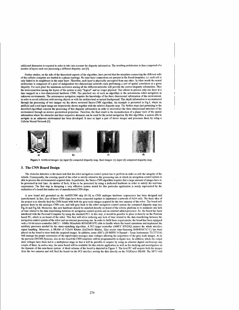
additional dimension is required in order to take into account the disparity information. The resulting architecture is thus composed of a number of layers each one processing a different disparity, see [1 j.

Further studies, on the side of the theoretical aspects of the algorithm, have proved that the templates connecting the different cells of this cellular computer are limited to a planar topology. No inter layer connections are present in the found templates, i.e. each cell is only linked to its neighbours in the same layer. Therefore, each layer is physically uncoupled from any other. In other words the neural architecture is composed of a pool of independent two-dimensional networks each performing a sort of spatial correlation at a given disparity. For each pixel the maximum activation among all the different networks will provide the correct disparity information. Thus the interconnection among the layers of the system is only "logical" and no longer physical. This allows to process only one layer at a time mapped on a two-dimensional hardware CNN. The practical use of such an algorithm is the autonomous robot navigation in unknown environments. The autonomous navigation requires the knowledge of the three dimensional information of the environment, in order to avoid collisions with moving objects or with the architectural or natural background. This depth information is reconstructed through the processing of two images via the above reviewed Stereo-CNN algorithm. An example is presented in Fig.l, where an artificial and a real input image are respectively shown together with the relative disparity map. The further steps (not pertaining to the described algorithm) concern the processing of this disparity information in order to reconstruct the three dimensional structure of the environment through an inverse geometrical projection. Therefore, the final result is the reconstruction of a planar view of the spatial information where the obstacles and their respective distances can be used for the actual navigation. By this algorithm, a system able to navigate in an unknown environment has been developed. It uses as input a pair of stereo images and processes them by using a Cellular Neural Network [5].

a) b) c) d)

Figure 1. Artificial images: (a) input (b) computed disparity map. Real images: (c) input (d) computed disparity map.

3. The CNN Board Design

The obstacles detection is the main task that the robot navigation control system has to perform in order so safe the integrity of the vehicle. Consequently, the cruising speed of the robot is strictly related to the processing rate at which its navigation control system is able to process the environmental acquired data. In particular, the Stereo-CNN algorithm requires that a large amount of images have to be processed in real time. As matter of facts, it has to be processed by using a dedicated hardware in order to satisfy the real-time requirement. The first step in designing a very effective system suited for this particular application is surely represented by the realization of a board that makes use of manufactured CNN chips.

A new board still grounded on the 6x6DPCNN chip [9-10] as CNN analogue hardware coprocessor has been designed and manufactured. In fact, four of these CNN chips have been connected together to implement a network of 6x24 cells. The basic idea of the project is to directly feed the CNN board with both the grey-scale images acquired by the two cameras of the robot. The board will process them by the analogue CNN core, and will give back to the robot navigation control system the computed disparity map (see Fig.lb and Fig.Id). Moreover, this new hardware should be installed directly on board of the robotic platform so to minimize any lack of time related to the data transferring between its navigation control system and an external added processor. So, the board has been interfaced with the Personal Computer by using the standard PCI. In this way, it would be possible to place it directly on the Pentium based PC, which is on board of the robot. This fact will allow reducing any lack of time related to the data transferring between the navigation control system of the robot and an external processing one. In order to fulfil these requirements, the board has been equipped with a 16-bit micro-controller (MCU - 16Mhz Mitsubishi M30624FGFP) able to handle whole the board operations and implement the auxiliary processes needed by the stereo-matching algorithm. A PCI target controller (AMCC S5920Q) assures the whole interface signal handling. Moreover, a SRAM of 512x16 Kbytes (2x256x16 Kbytes, 12ns access time-Samsung K6R4016C1C-C) has been placed on the board to store both the acquired images. In addition, some ADC's (20 MSPS 3-Channel - Texas Instruments TLC5733A) will manage the proper conversion of the input/output analogue state voltages allowing the acquisition of the grey scale images. As in the previous DPCNN Systems, also in this board the CNN templates will be programmable in digital way. In addition, whole the output state voltages have been led to a multiplexer stage so that it will be possible to acquire by using an external digital oscilloscope any couple of them. In such a way, the same board will be available for this robotic application as well as for studying and investigation on the dynamic of this non-linear system. A block scheme of the board is depicted in Figure 3. The host PC will acquire both the images from the two cameras and will feed the board via the PCI interface storing the data directly on the 512Kbytes SRAM. The MCU will

274

read the data on the SRAM and will transform them in a proper format able to feed the analogue CNN processing core. It is worth to note that because of the dimension of this analogue core the MCU has to handle the paging of the image to be processed. Successively, it will read the results from the CNN (i.e. the voltage steady states of the cells) and compute the disparity map giving back it to the host PC. The algorithm performed by the board is depicted in Fig.3.

a Rrtd be two

Mcmoiy(DRAM)

* ft * . :£9*&M:y;

4 » J

i **

Compute CNN

«NN \n*3 jt« « If

4> A f-1 1 **

<J L_ Chi

Ch?.

^~^ Analos 0 Outp,

DiUpiging (6x24)

ADC

1 1

U Store dit» in DPCNN core

CNNileidyitite

■ D»t»Bus

^ L_K> uv i 1 DATA

Memory (SRAM) MCU

JB DPCNN proevtang

Evaluto tbc Mix & build the

disparity map PCI

CorttraHfit Of Memory (FLASH)

* * <>n

1

N y\, J\

1 PCI Bus Y[ SwJ

DBP=DKP+1 t > i-<DlSP=10>-—»

Write the disparity map

in lie Memory (DRAM)

Figure 2. Block scheme of the board. Figure 3.Board algorithm.

Step Operation Estimated Processing time

1 Read Memory T, 2.88 ms

2 Compute CNN parameters T2 2.30 ms

3 Data Paging T, 0.63 (is

4 Store data in CNN analogue Core T4 70 (is

5 DPCNN analogue processing Ts 100 ns

6 AD conversion T, 74.4 ns

7 Evaluate Max & Build Disparity Map T, 180 ns

8 Write Disparity Map on Memory T, 90 ns

Single page processing time . Tpig, 515 ns

Single disparity plane processing time Tpiine 10.54 ms

8 Disparity planes Tpomc 87.24 ms (llF/s)

10 Disparity planes TPOBU 108.3 ms (9 F/s)

Where: Tpage = T3 +T< +T5 +T6+T7 +Tt; TP,aM = (TPage-\6)+T2; TFrame = (TPlane-ND)+Tl

In the previous table the estimanted processing time for each board operation have been shown. The expected processing time rate for a 48x48 pixels grey scale image will depend on the chosen maximum disparity level and will range from 9 to 11 frame /s for 10 and 8 maximum disparity respectively. Figure 4 the placement of the components in both the sides of the board has been shown.

275

4. Conclusions

The paper shows a new CNN board welt suited for the stereo vision algorithm. That board is based on the 6x6DPCNN chip will be installed directly onto the robot and take the role of a high performance neural analogue coprocessor able to processes in real time the stereo images. The processing rate performed by this board has been estimated in about 10 frame/s (for a grey scale image sized 48x48 pixels).

5. Acknolegments

This project has been partially funded by the Italian Ministry of Scientific Research (Projects PRIN-9809272019)

6. References

[1] A. Zanela, S. Taraglio, "Sensing the Third Dimension in Stereo Vision System: a Cellular Neural Networks Approach", Intern. Journal of Engineering Applications of Artificial Intelligence, 11 (1998), pp. 203-213.

[2] T. Poggio, V. Torre, C. Koch. "Computational vision and regularization theory1*, Nature, 317, pp 314-319, 1985. [3] L. O. Chua, L. Yang, "Cellular Neural Networks: Theory", Cellular Neural Networks: Applications IEEE Trans. Circuits and

Systems, Vol. 32, Oct. 1988, pp.1257-1272, pp. 1273-1290. [4] T. Roska, J. A. Nossek (Eds), "Special Issue on Cellular Neural Networks", IEEE Trans, on Circuits and Systems, Vol. 40, no. 3,

March 1993. [5] A. Zanela, S. Taraglio, "A cellular neural network stereo vision system for mobile robot navigation ", CNNA-2000. [6] S. Taraglio, A. Zanela, M. Salerno, F. Sargeni, V. Bonaiuto, "A CNN Stereo Vision Hardware System for Autonomous Robot

Navigation ", Proc. of CNNA98 5th IEEE Int. Workshop on Cellular Neural Networks and their Appl., London, United Kingdom, 1998, pp. 181-185.

[7] M. Salerno, F. Sargeni, V. Bonaiuto, S. Taraglio, A. Zanela, "A Dedicated Hardware System for Cnn Stereo Vision", IEEE International Conference on Circuits and Systems (ISCAS '99), Orlando, FL, USA 1999, Vol. VI, pag.501-504.

[8] M. Salerno, F. Sargeni, V. Bonaiuto: "A Dedicated Multi-Chip Programmable System for Cellular Neural Networks", Analog Integrated Circuits and Signal Processing, Kluwer Academic Publisher, Vol.18, no. 2/3, February 1999, pp. 277-288.

[9] M. Salerno, F. Sargeni, V. Bonaiuto, "6x6DPCNN: a programmable mixed analogue-digital chip for Cellular Neural Networks ", Proc. of CNNA-96 4th IEEE Int. Workshop on Cellular Neural Networks and their App!., Seville, Spain, 1996, pp. 451, 456.

[10] M. Salemo, F. Sargeni, V. Bonaiuto, "A 6x6 cells interconnection-oriented programmable chip for CNN\ Analog Integrated Circuits and Signal Processing, Kluwer Academic Publisher, Vol.15, no.3, March 1998, pp.239-250.

j » ,J, .;■: C « S i s * » * **

i~i~-f f. I: igt a t, ~:c

:;:** E« :::::: 3« it£ ■£;:: tS i: ••■::: s3 pi til.

>:■:».>:<) jBÄä*S«liw5 UKiMJÜJgW li£to*MfiM&ut KHM!*M*H«:

wn M hH. H* •** r* ?*s ../. y*s p? *^ tp» ^ £T:' fT-* ■j? fc 5; *;. *:• S-p ev. %u fc £. ff:. a;, o. v,-, if, '■

fife * l^l!"lPlfeflg|l-lPll g B " l|.,,.. sM 1 i*«' £:-r v w-r.T^w^ z'fpw' r s*lB" n fa"l Sa anjy?^. *i? ES KS irss A

.v:v.y.^^.-.!>?^.-.---..P-"

v v. 3!!;..;::";a: ■•• »t:«.;....it:... tit.........:» , HS::";::::!??' i,J:

et.

Figure 4. Top (a) and Bottom (b) component placement.

276

2000 6™ IEEE International Workshop on Cellular Neural Networks and Their Applications Proceedings

Low-Cost, High-Performance CNN Simulator Implemented in FPGA

Martin Perko, Iztok Fajfar, Tadej Tuma, Janez Puhan

University of Ljubljana, Faculty of Electrical Engineering, Trzaska25, 1000 Ljubljana, Slovenia

Phone: +386 61 1768 329 Fax:+386 61 1264 630

Email: martin.perko@fov.uni-mb.si

ABSTRACT: Recently, we proposed a concept of a non-microprocessor based CNN simulator [1]. An 8-bit FPGA based prototype of a 256 x 512 cell simulator is now fully operational and yields quite encouraging results. A 30MHz implementation in fact outperforms 200MHz Pentium based PC simulation. As some interesting solutions have been incorporated in the simulator design, this paper focuses on some aspects of implementation of the simulator.

Furthermore, several points where further optimisation of processes is possible at low cost have been discovered.

1 Introduction Cellular neural networks (CNN) are a powerful analogue parallel computing paradigm. There have been VLSI implementations of the paradigm with predictions of reaching 100 by 100 cell array in 1999 [4]. Many practical applications, however, call for larger arrays, and one has to resort to digital simulations, which are usually built using general purpose microprocessor or DSP [e.g. 3, 5].

For intensive computing applications, which a CNN simulator definitely is, a DSP is better choice. The reason is simple: it is dedicated to perform arithmetic operations and thus far more optimal for the task.

In this paper we present a different approach, which seems even more tailored for intensive computing involved in simulating analogue CNN operation.

Since the implementation is a prototype, it uses a FPGA chip as a core, but despite this fact it yields 370MIPS. Total chip cost is approximately $60 and theoretical logic power is 0.12 gates MHz. All features proposed in [1] (enhanced simulation and usage of non-standard time constants) have been included. Enhanced calculation is limited to two gains per cell, which gives gain errors up to 10%. As this design is a prototype, built in a tight FPGA, a flexible topology as proposed in [2] is not implemented. The final product is intended to be implemented in ASIC technology.

2 Theoretical Basics This chapter briefly summarises those theoretical aspects that have most impact on simulator implementation (refer to [1] for details).

Let us take the following difference equation, which describes dynamics of a cell in a CNN:

hl 9 h

(1)

Here, X(,„) and Y^n) are the state and output values of the r-th cell in n-th iteration. Note that state and output values are connected via a non-linear function/(*).

Constant factors k are obtained from elements of templates A and B (weights). As shown in [1], equation (1) can be recast into the following three equations, using partial state values.

Equation (2) describes gain (Go) generation of the Mh cell in the n-th iteration.

0-7803-6344-2/00/$10.00 ©2000 IEEE 277

Go(,,„) =(f(x'(,,B-i))-V(t.n_,))-— (2)

The gain depends on partial state value (Vo) and the state value (X) of the same cell. The partial state value is calculated as follows:

V°(,,n)=Vo(,,n-\)+G°(,,n) (3)

Finally, we can express the state value as a function of gains of the neighbouring cells:

9

*(l.»)-*(l.n-l) =*fG'(!,n) + X*'G0('..-.») (4)

Partial state values at steady state equal to the corresponding cell output value. The most important consequence of dividing equation (1) is the gain of the cell output value (2). In that way,

each cell in the array can be fed with the gains of its neighbours instead of complete output values. Due to the fact that the precision of gains does not impact the precision of state values in their steady state at

all, we can somewhat simplify them. We have chosen to limit the gains to assume the values of the form

2~",neN

Regardless of the number of bits used for input and output values, the maximum gain in every case equals to Vi. Its minimum, on the other hand, depends on the number of bits used.

Such design limits time constants hIC to V4, Vt and so on and yields gain errors up to 33%. However, both drawbacks can be easily overcome by using multiple gains as described in [1].

On the other hand, two great advantages stem from this change. Firstly, we reduced total width of interconnecting buses between cells, and secondly, greatly simplified implementation of multiplications.

3 Realisation of Calculations If we focus on a single cell, we see that the gain of each neighbour must be multiplied by the corresponding weight and added to the cell's state value. In turn, its own gain and partial state value must be calculated.

As the latter process requires the state value to be completely updated (all neighbouring cells' gains must be applied) with gains of the former iteration, it must be delayed for at least one row plus one more cell.

Therefore, we choose to split the described calculation into two operators: - OSCC, which calculates a new gain and partial state value. - NSCC, which is to complete the multiplications of neighbour cells' gains with the weights. Naturally, there are also other blocks, such as ISA management, sequencer, memory management units and so

on. However, they are not that important here and will be omitted. If we take a closer look on the bus requirements (which are usually a bottleneck) of each operator, we can

summarise that OSCC operator needs to read and write partial state (output) value, to write gain value and to read state value once per calculation.

NSCC operator, on the other hand, needs to read and write state value once per cell and to read gains 10 times (9 feedbacks and an independent input) per cell.

It is obvious that NSCC operator is far more critical than OSCC.

3.1 The NSCC Operator

As we mentioned before, the NSCC operator must complete 9 multiplications and additions per cell. Hence, the first step of designing this operator must be an optimisation.

As in fact two neighbour cells share 6 out of 9 gains, the NSCC operator must only read the new 3 gains for each new cell it starts to calculate as seen in Figure 1. Of course, the shared gains must be multiplied by different weights for cells n and n+1. If we observe the gain in cell, marked with x in Figure 1, we can conclude that it

278

should be multiplied by weight A(0,-1) by NSCC when calculating the new state value of the «-th cell. Otherwise, it should be multiplied by weight A(-l,-l) for the n+1 th cell.

Note that the weights are elements of a feedback template A as described in [ 1 ].

NSCC operator n NSCC operator n+1 gain usage gain usage

X

n-. ■ Ai MOfipJ.

: i

shared gains

Figure 1: Shared gains for two successive cells

Should we disregard the fact that a majority of gains are shared, the NSCC operator would have to read all 9 gains for each new cell.

In reality, the NSCC operator consists of three shift registers and adders as depicted in Figure 2.

col.O col. 1 col -1 weights weights weights

gains in >1 a a*

| *o 1 1 ■o 1 I shift shift shift

register register register u Lr Lr state in

adder - dder - adder - s

"" T I1"" -i^- Y

out state

Figure 2: Structure of the NSCC operator

The gains enter to the operator in columns. That is, at the same time with the n-th state the gains of n-th cell and of its upper and lower neighbour cells arrive.

Hence, for each new input state three gains arrive to the operator and each adder must sum up three numbers. That can be done either by using three adders and shift registers per column or by sequencing the calculations. Due to limited gate count of the target device selected, we have chosen the latter option.

At clock frequency of 30MHz a cell is calculated in 100ns. The topology described in Figure 2 is valid only for basic simulation. When multiple gains are using in order

to reduce computational errors, some delays are reorganised as follows in Figure 3.

col. 0 col. 1 weights weights

col.-l weights

gains in T3

| | u •a

.3 1 1 1 1 1 1 shift

register

adder V-

shift register

adder r~

shift register

state in h "3

L adder p J2

-" T 1 ■-*• ^^T state out

Figure 3: NSCC operator topology for enhanced simulation

279

In that case, the same state value enters to the state in input twice. At the first time, it is accompanied by gains as described before. At the second time, the enhancement gains come along. Naturally, the entering enhancement gains are from the same column as the basic ones. In this case, 200ns is required at clock speed of 30MHz to calculate one cell.

In both cases, the shift registers act as multipliers of weights by gains.

3.2 The OSCC Operator

As stated before, the OSCC operator is not so critical. Its simplified structure is shown in Figure 4. The presettable nonlinearity is in fact a limiter with presettable upper and lower limits. Thus, the classical

sigmoid function can be achieved.

stale in presettable nonlinearity

adder

r gain

generator output in

N r output out

Figure 4: Structure of the OSCC operator

The switch is in the shown position when calculating basic gains (either in classic simulation or in the first step of enhanced one). In the second step of enhanced simulation (when calculating enhancement gains), however, it is switched to the other position. Becouse the OSCC and the NSCC operators share the same clock, the former one would furnish a new result every 33ns at 30MHz system clock. But as the NSCC operator requires 100ns, such speed would be an overkill. Therefore, the OSCC operator is allowed to take 3 clock periods (100ns) to calculate the result.

4 Physical Implementation The core of the simulator is Xilinx Spartan XCS30-3 FPGA which proved to be just of the size to hold all of the simulator components.

All memories are generic 128k x 8 asynchronous static memories with access time of 20ns. The simulator is designed to be used with a personal computer via ISA bus. This bus was selected due to easy

prototyping and possibility of selecting cheaper components. Unfortunately, its speed (a few megabytes per second) represents severe drawback.

5 Performance Analysis Naturally, it is important to determine what the simulator is capable of. In the following table, all operations needed to calculate a cell value using a straightforward difference equation calculation are summarised.

Multiplications (weights) 10 Mutiplications (other) 1 Summations (weights) 10 Summations (other) 3 Memory transfers (inputs) 1 Memory transfers (outputs) 1 Memory transfers (states) 9 Comparations 2

Therefore, a classical simulator has to complete at least 26 arithmetic operations and 11 memory transfers to complete one cell calculation. A total number of instructions is therefore 37. As our simulator calculates one cell in 100ns, this means that we have achieved 370 millions of equivalent operations per second.

The most important advantage, however, lies in the future. The diagrams on the following two figures explain this assertion.

In Figure 5 we see a comparison of number of flip-flops (FFs) needed for a proposed and standard implementation.

280

The reason for such difference is simply the fact that gate count in the proposed concept raises approximately

by N ■ log 2 N , whereas in the classic concept it raises approximately by N , where N is the number of bits used

for input and output words. A diagram in Figure 6 shows that a similar effect can be observed in bus widths. This difference is not so

important as the former one because the diagram includes all memory transfers. Many of them, however, can be eliminated using cache memory.

Nevertheless, we can conclude that the proposed concept is well prepared for long data words.

14000

12000

10000

8000

6000

4000

2000

0 0 32

■FFs proposed 64

Bits 96

FFs classic

Figure 5: A FF counts comparison

128

1400

1200

1000

800

600

400

200

0 0 32 64 96

— Proposed Bi,s

- - Classic

Figure 6: Total bus width comparison

6 Conclusions Our simulator is capable of processing all CNN operations where dynamic behaviour is not extremely critical. Even in those cases one can perform an enhanced simulation and get satisfactory results.

Nevertheless, some points of optimisation still exist. Perhaps the most important of all would be implementation of level one cache. Should a 2.5kb internal multitap cache memory be incorporated, the simulator would be able to achieve 14milions cells/iterations per second using classical 60ns EDO dynamic memories with no external cache. This means almost 520 equivalent MIPS. In this case, gate count would rise to approximately 18000.

The second optimisation concerns the nature of some applications. A lot of image processing operations (e.g. hole filling) suffer from high "dummy calculation" rate. That is, a lot of cells have the same state value before

281

and after calculation. Therefore, a preliminary identification of cells that will not change in the next iteration is necessary. Since, for example, connected component detection on 512x256 array includes only 3% of cells that do change their values in certain iteration, even a low hit-rate identification would save a lot of time.

As in our concept the change of a cell state value is determined solely by magnitude of gains of its neighbours, it is quite simple to determine in most cases when the state value does not change. Namely, it does not change if all gains of its neighbours equal to zero.

7 References [1] M. Perko, I. Fajfar, "Proposal for implementation of digital non-microprocessor based CNN simulator,"

ECCTD-97, vol. 2, pp. 609-615, August 1997 [2] M. Perko, I. Fajfar, T. Tuma, J. Puhan, "Fast Fourier transform computation using a digital CNN simulator,"

CNNA-98, pp. 230-235, April 1998 [3] R. Kunz, R. Tetzlaff, D. Wolf, "SCNN: a universal simulator for cellular neural networks," CNNA-96, pp.

273-278,June 1996 [4] T. Roska, "Analogic CNN computing: architectural, implementation and algorithmic advances - a review,"

CNNA-98, pp. 3-10, April 1998 [5] B. Feher, P. Szolgay, T. Roska et al, "ACE: a digital floating point CNN emulator engine," CNNA-96, pp.

273-278,June 1996

282

2000 6™ IEEE International Workshop on Cellular Neural Networks and Their Applications Proceedings

Object Oriented Image Segmentation on the CNNUC3 Chip P. Földesy, G. Lihan, A. Rodriguez-Vazquez, S. Espejo and R. Dominguez-Castro

Instituto de Microelectrönica de Sevilla - CNM-CSIC, Edificio CICA-CNM, C/Tarfia s/n, 41012- Sevilla, SPAIN Phone: +34 95 4239923, Fax: +34 95 4231832, E-mail: peter@imse.cnm.es

ABSTRACT: In this paper we show how a complex object oriented image analysis algorithm can be implemented on a CNNUM chip for video-coding. Besides the applied linear opera- tions, several gray-scale non-linear template operations are also emulated using algorithmic solutions.

1. Introduction*

Cellular Neural Networks (CNNs) [1] exhibits outstanding image processing capabilities. With the extension of this processing core first to the CNN Universal Machine [2], and, then towards a complex image processing system - the CNN Chipset Architecture [3] - these capabilities can be utilized in real-life applications. However, feasibility of the technology is strongly dependent on the availability of high-performance customized mixed-signal chips like the one described in [5] and [6].

In this paper we demonstrate the use of CNN-UM chips for implementing object segmetation in real-time. Object-based image and video processing represents the latest revolution in the field of computer vision. Scenes are no more simply addressed as a set of pixels or block of pixels, but as a set of objects. This approach provides new solutions for a wide range of applications from automatic surveillance to video stream coding. The implemented algorithm is based on the work of [4] with several improvements.

The experimental results have been processed by the so-called CNNUC3 (or 64 x 64FPAPAP) CNN-UM chip [6]. The chip comprises a 64 x 64 pixel array with gray-scale input and output CNN core, extensions to direct opti- cal input, fixed-state mask, arithmetic unit, etc. It has been manufactured in 0.5um standard CMOS technology with almost 1 million transistors 80% of which operate in analog mode; the remaining 20%, used for programming, memory and control operate in digital mode.

2. Implementation

2.1 Introduction In this section we review the goals and the main features of the segmentation algorithm. The method employs

luminance contrast (low-spatial freqencies), luminance gradient (high-spatial freqencies), and consequtive frame difference (or motion) information. Besides the realization on the CNNUC3 chip, the algorithm reported in [4] has been improved as follows:

• usage of robust operations and misusage of not-terminated transients (only dc outputs), • segment any of the possible objects regardless to their motion by improved intraframe segmentation,

• mark the moving objects, • restoring of the moving object contours without degradation, • avoid the need of intermediate frames between the coded ones.

After gray-scale preprocessing, three types of information are gathered: (i) contour estimation by thresholded gradient and by (ii) edges of similar luminance level areas, and (iii) thresholded frame difference. Next, this infor- mation is merged and filtered by morphological operators. Then the smaller and larger objects are separated. The final segmentation contains the external contours of the larger objects, and the skeleton of the thinner ones. We tried to use as many contour information as possible and not to destruct them by the unaviodable binary filtering. The flow-chart of the whole process can be seen in Fig.l.

In the following sections, details of each step are described with special care to the algorithmic solutions of gray-scale nonlinear operations.

2.2 Edge-Enhancing Low-Pass Filtering, Thesholded Gradient

First, the high-frequency noise component is reduced by a linear low-pass filtering, which contained an image-smoothing B and a Laplacian-like A template. This operation besides the noise suppression, also blurs the

t. This work has been partially funded by ONR-NICOP N68171-98-C-9004, DICTAM 1ST-1999-19007 and TIC 990826.

0-7803-6344-2/00/SlO.OO ©2000 IEEE 283

object edges. In order to enforce the noise reduction while maintaining the edge structure, a gradient controlled low-pass filtering is used (anisotropic diffusion). Since this operation is generally highly non-linear, a simple algo- rithmic replacement is applied (and can be renamed as nonlinear diffusion). The algorithm comprises blurring, gra- dient calculation utilizing the piecewise linear output tramsfer function, and extensive usage of the fixed-state map to handle separately the edge-like areas. The block diagram of the algorithm can be seen in Fig.2. and the processed two sample frames in Fig.3.

I Actual frame

bdge-enhancing Low-pass Filtering

jE

Filtered image Previous frame

Ihresholded Uradient II Luminance Contours S Frame Üitterence

Merging

T T Moving Regions

I Small Object Removal I

Region Size Classification I bdge Extraction I

Large Objects I I Thin Objects Skeletor I bdge Extraction II skeletonization U

I Merging U

* * Object Contours Moving Objects Region

Fig. 2: The block diagram showing the implemented segmentation algorithm.

Uradient in one direction, high offset to drive negative

values to white

x4

C~Partial result j

Input

m lJl Uirtusion

£ Uradient Calculation

3 Ihrcshold 2"J L)ifi

Logic Inversion

* As Fixed-stale mask

'S"1 Diffusion

Contrast Enhance

' Uirtusion **-

^ Output J

Fig. 2: The block diagram of the edge-preserving low-pass filter implementation can be seen in the figure. It supresses the separated edges and low intensity noise, while preserve the real edges. In the gradient calculation the sobel operator was used rotated in four directions. The role of the last three steps of diffusion and contrast enhance is to remove the noise from the edge areas and eliminate the unconsistancy between the edge and the remaining areas.

2.3 Motion Detection

In order to invoke the motion information the pixelwise image different between two frames is calculated. In contrast to the published method, we used double thresholding on the difference instead of absolute value calcula- tion and thresholding. In this way, the appearing and dissapearing light and dark areas can be distinguished and merged the proper one with other object information regarding to the current frame. This separation is useful because the raw difference contains information about two frames.

We found that the contours extracted by thresholded gradient can be correlated well with the appearing and dis-

284

Fig. 3: In the images the results of the implemented nonlinear diffusion. Image (a) is the 65 frame of the "miss america"

video sequence. Image (b) is the same frame after processing, and image (c) is the processed 85[ frame of this sequnce.

I, Actual frame Previous frame

xternal Pixel Count

W MUX Kr

"IT" "OTT

(a)

,\Ml.

ifcv (b)

(d) fJ !v (c)

Merged Object regions (d)

Fig. 4: The block diagram of the motion detection. The contour information of the threshhlded gradient operation is correlated with the appearing and dissappearing areas. Which area contains the more common information is merged with the contours. The images on the right side show partial results denoted by letters, which can be found also in the flow-chart.

sapearing regions. After binary correlation the evaluation is done externally by counting the black-and-white pixel ratio of the results. See Fig.4. for the flow-chart of this process.

2.4 Intensity Contour Detection

The contour estimation by the thresholded gradient is working only in cases where edge regions are sharp enough. It is not always true in natural environment, and the contours can be broken and not closed. On the other hand the luminance information diffused in regions can give this lack of information.

First, an extenal processor calculates the histogram of the incoming images dividing the luminance swing into 8-32 levels (this process is not need extensive calculations by the digital counterpart of the CNN chip). With this information some levels are choosen at the local minimums of the histogram where the preprocessed image is thres- holed. With this threshold level choise, the similar large areas are not segmented.

After smoothing and edge detection on the binary results, closed and mostly not oversegmenting borders can be extracted. The corresponding results can be seen in Fig.5.

285

Fig. 5: In image (a) the result of the intesity based edge detection, in image (b) the result of the thresholded gradient, and in image (c) merged images can be seen.

2.5 Moving Areas, Filtering

The total area of movement is extracted as follows. The three main type of information is merged in this step and whole filling the outer parts of the frame is cleared. Using the binary contours of these image, the existing con- tour estimation can be enhanced.

The next step is the small object removal and the internal whole filling. In these steps morphological operators or hole filling with the commonly applied "hollow" function [7] cannot be used without some additional restriction because it may merge separable objects or destruct edge structures. To overcome this problem we use the fixed state map. This contains the combination of the enhanced contour estimation and the inverted moving area map (the still background). By freezing the existing contours and background the above mentioned operations can work safely.

Object size classification is used for small object removal, because the available one-template operations also could destruct the contour structure. In this step and in the laters, it is done by multiple morphological erosion and reconstruction.

The results of the moving area detection and this filtering can be seen in Fig.6.

(a) (b) (c)

Fig. 6: The moving regions, the enhanced contour estimation, and this image after whole filling and small object removal can be seen in the images.

2.6 Final Contour Extraction

In this part of the algorithm, the goal is to maintain the external borders of the moving segments, create exact contours of the larger objects, and limit the processing time of the applied skeletonization cycles.

In order to distinguish the objects, size classification is used as was mentioned above. The smaller objects (see Fig.7a,b) are removed and stored for later edge extraction, while the remaining larger ones are processed next. Dur- ing the object classification, after the morphological erosions, a so called "core" remains (see Fig.7c) before the reconstruction step. This core is increased (see Fig.7d) in the same amount then the erosion was applied, results in large, not connected objects. This result is also stored for later edge extraction.

286

If this core is removed from the original image, an edge-like image is the result with several pixel width (see Fig.7e). This image is the input of the following skeletonization process, granting the finite process time. In order to maintain the external borders of the moving region, the fixed state map is used. The input of the skeletonization is the logic combination of the thick edge map and the still background map. During the skeletonization, this back- ground stops the peeling at the required borders. The skeleton in this way represent the internal edges, but follows the previously found external borders.

When the skeleton is ready (see Fig.7f), the background is removed, the previous small and large regions are added (see Fig.7g), and the last edge detection of this combination provide the final result (see Fig.7h).

<d> + y

A3 <r ̂

, V l (g) <h)

Fig. 7: Examples of the final contour detection can seen in the images. See text for detailed description.

2.7 Comments

As a result, the image containing the segment borders can be processed externally by later high-level labelling and tracking. The final segmented images can be seen-in Fig.8. These example frames were choosen quite far from each other (representing a 3 frames/sec rate) in order to show the consistance of the segmentation.

The total number of template executions and logic operations in the algorithm is maximum 90 and 15, respec- tively. When the processed frames are the size of the chip (64 x 64 pixels), the required time of the processing with- out the I/O time is approximately 2msec. The memory management of the implementation was optimized, and since the chip contains 4 LAMs, 4 LLMs, and additional capacitances for memory interchange, all of the image process- ing steps of the algorithm can be executed within the chip without external storage.

In case of QCIF (176x144) sized images the 30 frames/seconds rate can be achived. It should be mentioned that the segmentation of large images into chip sized parts also includes additional image transfers in order to maintain the consistancy of the frame. But this process occures in our case only for binary images, and the overhead is slight.

2.8 Future Work

In the future exhastive test is intended to be done. The algorithm is known to fail when the background has sim- ilar contrast and intesity information that the moving objects, and itself is also changing. The solution for a more general process requires motion estimation and the preliminary knowledge of the higher level algorithms, which use the information of the segmentation. See [8] for an other survey based on global optimization technics.

287

3. Conclusion

We implemented a object segmentation algorithm on the CNNUC3 chip. We used robust operations, image inde- pendent processing time, and solved several drawbacks of a known method. The estimated frame rate is 30 frames/sec on QCIF images.

It also became clear that the image processing capability of the CNN architecture can be optimized in the system level when conventional digital coprocessors are also present with the proper division of the tasks.

4. References

[1] L.O. Chua and L. Yang, "Cellular Neural Networks: Theory". IEEE Trans. Circuits and Systems. Vol. 35, pp. 1257-1272, Oct. 1988.

[2] T. Roska and L.O. Chua, 'The CNN Universal Machine: An Analogic Array Computer". IEEE Trans. Circuits and Systems //, Vol. 40, pp 163-173, March 1993.

[3] T. Roska , "CNN Chip set Architectures and the Visual Mouse". Proc. of the IEEE CNNA-96. Seville, pp. 487-492. 1996. [4] A. Stoffels, T. Roska, and L.O. Chua, "Object Oriented Image Analysis for Very-low-bitrate Video-Coding Systems, using

the CNN Universal Machine", Int. Journal on Circuit Theory and Applications. Vol. 25, pp. 235-258,1997. [5] R. Domfnguez-Castro, S. Espcjo, A. Rodrfguez-Väzquez, R. A. Carmona, P. Foldesy, A. Zarandy, P. Szolgay, T. Sziranyi

and T. Roska, "A 0.8um CMOS Two-Dimensional Programmable Mixed-Signal Focal-Plane Array Processor with On-Chip Binary Imaging and Instructions Storage". IEEE Journal of Solid-State Circuits. Vol 32, pp 1013-1026, July 1997.

[6] G. Linän, S.Espcjo, R. Domfnguez-Castro and A. Rodrfguez-Väzquez., "The CNNUC3: An Analog I/O 64 x 64 CNN Uni- versal Machine Chip Prototype with 7-bit Analog Accuracy". Proc. of the CNN2000. submitted.

[7] T. Roska, L. K6k, L. Nemes, Ä. Zarändy, M. Brendel, CSL - CNN Software Library, Version 7.2 DNS-CADET-15. Analog- ical and Neural Computing Laboratory, Computer and Automation Institute, Hungarian Academy of Sciences, Budapest, 1998.

[8] T. Sziränyi, K. Läszlö, L. Czüni and F. Ziliani, "Object oriented motion-segmentation for video-compression in the CNN-UM". Journal of VLSI Signal Processing November 1999.

288

2000 6™ IEEE International Workshop on Cellular Neural Networks and Their Applications Proceedings

Structure Reconfigurability of the CNNUC3 for Robust Template Operation P. Földesy, G. Lindn, A. Rodriguez-Vazquez, S. Espejo, and R. Dominguez-Castro

Institute de Microelectrönica de Sevilla - CNM-CSIC, Edificio CICA-CNM, C/Tarfia s/n, 41012- Sevilla, SPAIN Phone: +34 95 4239923, Fax: +34 95 4231832, E-mail: peter@imse.cnm.es

ABSTRACT In this paper we demonstrate the importance of the reconfigurabilitiy of a 64x64 cells size CNN-UM chip. As we show, in such a high complexity mixed-signal VLSI circuit the switch and internal reference level reconfigurability and reprogrammability play a crucial role for the robust operation of the system. The methodology for exploring the possibilities is three-fold, we consider theoretical results, error compensation methods, and the usage of special features of the design.

1. Introduction*

It is widely accepted that Cellular Neural Networks [ 1 ] exhibit outstanding image processing capabilities when compared to conventional purely digital approaches. In fact, despite their simple local non-linear dynamic evolution CNNs are able to implement a vast set of complex image processing functions with a processing speed incompara- bly higher than their digital counterparts. The key for this result is the parallel computation that could be simply defined as let all the cells (pixels) to process by themselves at the same time, therefore, the computing power of a specific CNN implementation depends directly on the number of cells in the array. For that reason, the natural trend for many years in the silicon implementations have been the increase of the number of neurons in the chips.

Nevertheless the increasing complexity of CNN implementations strongly implies the usage of robustness ori- ented architectures and circuit design techniques. In that sense, several approaches and solutions have been pub- lished. This paper presents some topics on robustness increase that have been implemented in a new analog-input analog-output 64 x 64 CNN chip called CNNUC3 [2]. The basic idea for solving some inaccuracies and to explore for new operations is the free reprogrammability of the switches that control the data transferences and the flow of the processes.

This paper is organized as follows: Section 2 briefly presents the chip architecture, the cell block diagram and the implemented state equation. Section 3 presents two general aspects to increase the template robustness while Section 4 presents two special functionalities added to the CNNUC3 prototype, namely the possibility of reconfig- uration for implementing differential convolutions and that for DTCNN operation.

2. Chip Description and State Equation on CNNUC3

As most CNN chips, the CNNUC3 prototype, can be basically described as an array of identical cells, whose main function is to perform CNN operations on images (pixel arcays) of the same size (64 x 64 ). The implemented CNN algorithm is continuous-time, spatially-invariant, with linear template elements, and a radius-1 neighborhood, while the CNN state equation follows the so called Full Signal Range model (FSR) [3]. All elements of the feedback and control templates, as well as the bias (or offset) term, are programmable with a resolution of seven bits plus sign. From an external point of view, images may be analog (gray-scale), binary (black & white), or they can be directly captured by using the gray-scale photosensor included within each cell. Internally, from a CNN processing perspective, pixel values are treated as analog in general, with black & white images having extreme analog levels corresponding to the limits of the linear region. However, specific memories and some logic processing functions are included for binary images. Image storage is possible in both analog and binary form.

The cell array comprises the 64 x 64 inner cells and a surrounding ring of border cells used to establish the necessary spatial boundary conditions for CNN processes. Other miscellaneous functions like analog and digital buffering, control, and I/O tasks, are also included within the border cells. In addition to the network circuitry, the prototype includes some global control and programming circuitry located in the periphery of the cell array. This includes memory for 32 arbitrary sets of CNN coefficients, which after being programmed can be arbitrarily selected from the outside. Some other analog values related to the CNN processing circuitry, like the limits of the

t. This wo* has been partially funded by ONR-NICOP N68171-98-C-9004, DICTAM IST-1999-19007 and TIC 990826.

0-7803-6344-2/00/S10.00 ©2000 IEEE 289

linear region and others, can also be programmed. Digital to Analog (DA) converters generate the analog-program signal levels transmitted to the cell array from the selected set of coefficients.

Fig.l (a) shows the chip architecture, the prototype incorporates some global-control and programming circuitry located in the periphery of the array. This includes memory for 32 arbitrary sets of CNN coefficients and for 64 arbitrary sets of 35 digital signals that are used as digital instructions to configure properly the cell in order to perform different task ranging from running a CNN process to configure the cell I/O circuitry. These memories can be randomly addressed from the hosting platform once they have been programmed. Fig.l (b) shows the chip microphotography.

Analog j/Q^Data bus . M r3

3 CELL ARRAY Ofl

PROGRAMM. CIRCUITRY

^

Digital I/O Data bus

Fig. 1: (a) Chip Architecture.

1 p~. i,^m»^m^smm :

9.145mm

Fig. 1: (b) Chip Microphotography.

Fig.2 shows the basic structure of a template execution core containing the convolution masks, the possible input sources, the insertion point of the fixed-state mask, and a synapse current calibration circuit. The data and operation flow is controlled by several switches and reference values. A general template execution contains up to two cali- bration phases, initial state and input capacitor initialization, transient evolution, and result storing. During the cal- ibration the convolution sum of the used template and the mid-gray (zero) level is stored as a reference for the image processing. In the transient evolution phase, this sum is subtracted from the incomi

ng synapse current producing the current that is integrated in the state capacitor.

zero level LLM LAM

fixed slate map in LLM3

Fig. 2: The structure of the cell processing core of a cell in the CNNUC3 chip.

This differential structure allows a high-precision opcration.The result of the transient evolution can be stored in any of the Local Memories of the cell, either analog or digital.

Equation (1) shows the state equation of the cells including the calibration sum (note that the cells have been designed using the full-signal range (FSR) model [3]).

290

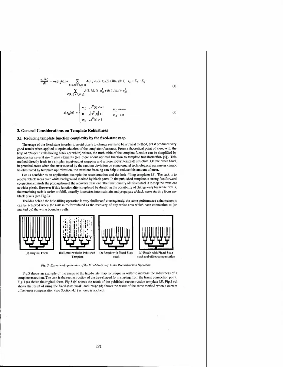
dx'Kt)

C»,0sS,(i,')

O.k. I) 6 S,(i, J)

(1)

«[*,/'>]

mL ,*"(() <-l

o , lAol < 1 mR ,x\t)>\

(2)

3. General Considerations on Template Robustness

3.1 Reducing template function complexity by the fixed-state map

The usage of the fixed state in order to avoid pixels to change seems to be a trivial method, but it produces very good results when applied to optimatization of the template robustness. From a theoretical point of view, with the help of "frozen" cells having black (or white) values, the truth-table of the template function can be simplified by introducing several don't care elements (see more about optimal function to template transformation [4]). This method directly leads to a simpler input-output mapping and a more robust template structure. On the other hand, in practical cases when the error caused by the random deviation on some crucial technologycal parameter cannot be eliminated by template optimization, the transient freezing can help to reduce this amount of error.

Let us consider as an application example the reconstruction and the hole-filling templates [5]. The task is to recover black areas over white background marked by black parts. In the published template, a strong feedforward connection controls the propagation of the recovery transient. The functionality of this control is to stop the transient at white pixels. However if this functionality is replaced by disabling the possibility of change only for white pixels, the remaining task is easier to fulfil, actually it consists into maintain and propagate a black wave starting from any black pixels (see Fig.3).

The idea behind the hole-filling operation is very similar and consequently, the same performance enhancements can be achieved when the task is re-formulated as the recovery of any white area which have connection to (or marked by) the white boundary cells.

Wy •i.'iliihü!::: iüiüjllll'i" ■iiii!n:;i!ü¥

(a) Original Form (b) Result with the Published (c) Result with Fixed-State (d) Result with Fixed-State Template mask. mask and offset compensation

Fig. 3: Example ofapplication of the Fixed-Stale map to the Reconstruction Operation.

Fig.3 shows an example of the usage of the fixed-state map technique in order to increase the robustness of a template execution. The task is the reconstruction of the tree-shaped form starting from the frame connection point. Fig.3 (a) shows the roginal form, Fig.3 (b) shows the result of the published reconstruction template [5], Fig.3 (c) shows the result of using the fixed-state mask, and image (d) shows the result of the same method when a current offset error compensation (see Section 4.1) scheme is applied.

291

3.2 Strong negative self-feedback in uncoupled templates

It is well known that negative feedback increases stability and robustness of any system. In this section the importance of negative self-feedback for robust template operation is demonstrated through experimental results. The analysis of the dynamic routes of the state variables demonstrates that negative self-feedback produces an unique (not bistable nor time dependent) equilibrium point at the end of the transient evolution of the network. Fur- thermore, this equilibrium point does not depend on the initial value of the state variable, consequently, all the prob- lems arising from the initialization of the CNN transient can be neglected.

Two important reasons for using negative self-feedback even in binary output cases can be found. • In high-speed VLSI implementations the time constant of control signal propagation and reference level

distribution is in the range of the cell time constant. Hence the initialization of CNN transient evolution can be disturbed by mean of clock signal cross-talk or voltage drop on the reference levels. It causes that the cells will slightly behave differently depending on their position in the cell array. Or with other words, the robustness of the operation decreases in an unpredictable manner. In order to avoid the initialization problems the value of the output should not depend on the initial conditions of the cells. Or, the used template should guarantee its insen- sitivity.

• The negative self-feedback compresses the voltage swing of the integrated synapse currents. This phenom- enon also helps to increase the working precision because higher values on the template elements can be used thus increasing the signal-to-noise (here noise refers to either electrical noise and spatial noise).

^

1 1 !_'_": A , -\ -A P

-■> i i ^ . 7 A

•-. : . / '--VA ! 1. '.-• m/,^m

(a) Input Image

Fig. 4: Example of the usage of negative self-feedback in a high-pass filtering process.

(b) Small negative self-feedback

(c) Large negative self-feedback

Fig.4 shows the application of negative self-feedback for the high-pass filtering operation in gray-scale input images. The used image size is 176x144 pixels (QCIF) and was divided into chip nine overlapped pieces to fit the chip size. Producing a black and white image containing only the edges on the input image from the result in Fig.4(c) only requires a thresholding process.

4. Two Spetial Functionalities on CNNUC3

4.1 Differential input convolution

The first circuit specific extension that we present is the change of the role of the synapse current calibration circuitry. Since this current memory is not restricted inherently to provide the zero offset current that correspond to the zero input level, it can be used to store the convolution sum of non-zero images. Therefore, it is possible to per- form fully differential input convolutions that cannot be implemented on the original CNN-UM architecture [6J.

The original intended values for the parameters u , u in equation (1) were the uniform analog zero level for input and state variables. However if their values are changed to meaningful pixel values, the differences among the two pixels become the argument of the applied convolution mask. Applications of this enhanced functionality are the possibility of having linear arithmetic operations using analog images. Among those operations, the substarction

292

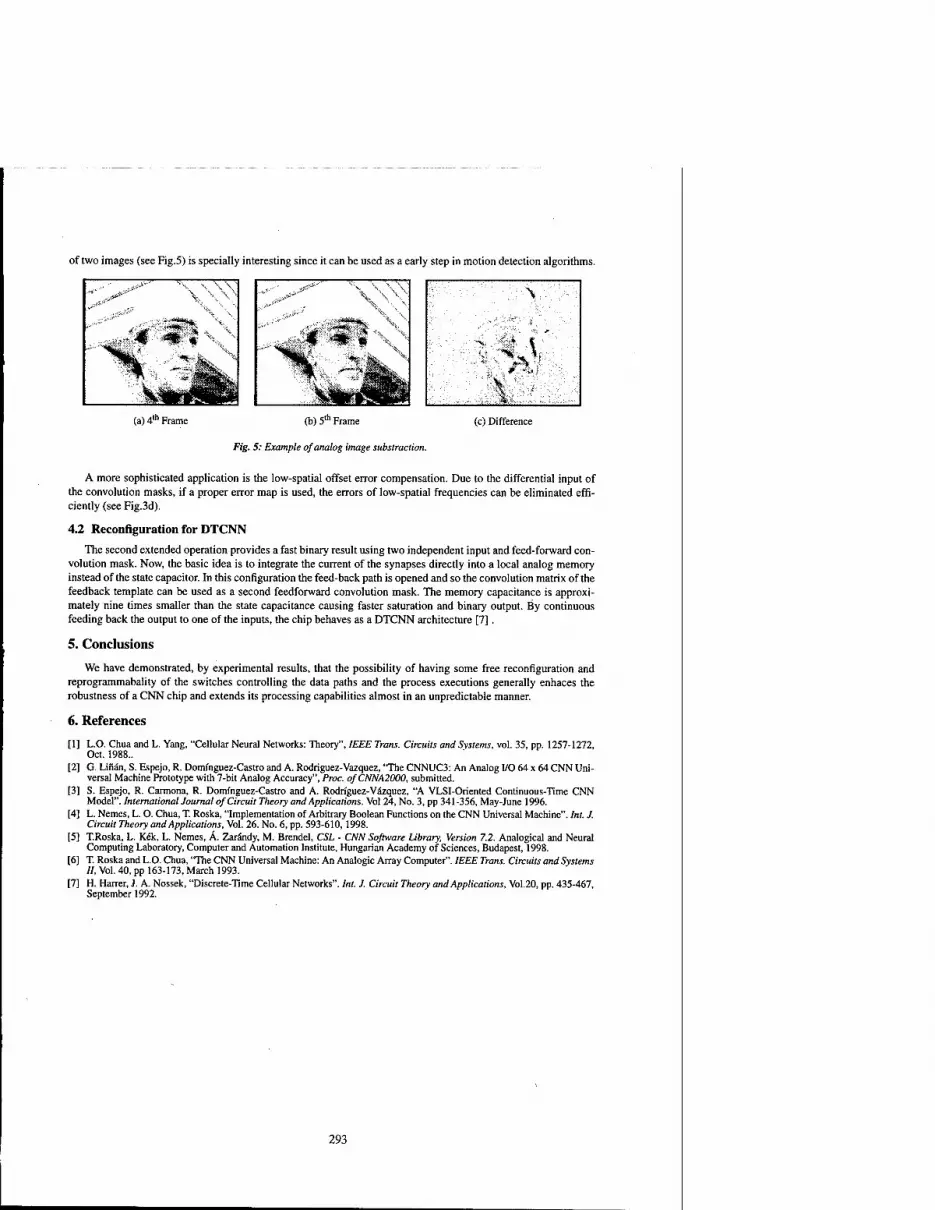
of two images (see Fig.5) is specially interesting since it can be used as a early step in motion detection algorithms.

V-'

V 'S >v' X

(a) ^ Frame (b) 5* Frame

Fig. 5: Example of analog image substruction.

(c) Difference

A more sophisticated application is the low-spatial offset error compensation. Due to the differential input of the convolution masks, if a proper error map is used, the errors of low-spatial frequencies can be eliminated effi- ciently (see Fig.3d).

4.2 Reconfiguration for DTCNN

The second extended operation provides a fast binary result using two independent input and feed-forward con- volution mask. Now, the basic idea is to integrate the current of the synapses directly into a local analog memory instead of the state capacitor. In this configuration the feed-back path is opened and so the convolution matrix of the feedback template can be used as a second feedforward convolution mask. The memory capacitance is approxi- mately nine times smaller than the state capacitance causing faster saturation and binary output. By continuous feeding back the output to one of the inputs, the chip behaves as a DTCNN architecture [7].

5. Conclusions

We have demonstrated, by experimental results, that the possibility of having some free reconfiguration and reprogrammabality of the switches controlling the data paths and the process executions generally enhaces the robustness of a CNN chip and extends its processing capabilities almost in an unpredictable manner.

6. References

[1] L.O. Chua and L. Yang, "Cellular Neural Networks: Theory", IEEE Trans. Circuits and Systems, vol. 35, pp. 1257-1272, Oct. 1988..

[2] G. Lilian, S. Espejo, R. Domfnguez-Castro and A. Rodriguez-Vazquez, "The CNNUC3: An Analog I/O 64 x 64 CNN Uni- versal Machine Prototype with 7-bit Analog Accuracy", Proc. ofCNNA2000, submitted.

[3] S. Espejo, R. Carmona, R. Domfnguez-Castro and A. Rodriguez-Vazquez, "A VLSI-Oriented Continuous-Time CNN Model". International Journal of Circuit Theory and Applications. Vol 24, No. 3, pp 341-356, May-June 1996.

[4] L. Nemes, L. O. Chua, T. Roska, "Implementation of Arbitrary Boolean Functions on the CNN Universal Machine". Int. J. Circuit Theory and Applications, Vol. 26. No. 6, pp. 593-610,1998.

[5] T.Roska, L. Kek, L. Nemes, Ä. Zarändy, M. Brendel, CSL - CNN Software Library, Version 7.2. Analogical and Neural Computing Laboratory, Computer and Automation Institute, Hungarian Academy of Sciences, Budapest, 1998.

[6] T. Roska and L.O. Chua, "The CNN Universal Machine: An Analogic Array Computer". IEEE Trans. Circuits and Systems II, Vol. 40, pp 163-173, March 1993.

[7] H. Harrer, J. A. Nossek, "Discrete-Time Cellular Networks". Int. J. Circuit Theory and Applications, Vol.20, pp. 435-467, September 1992.

293

2000 6™ IEEE International Workshop on Cellular Neural Networks and Their Applications Proceedings

Massively Parallel Processing Implementation of the

Toroidal Neural Networks

P.Palazzari'.M.Coli2, RRughi2

'ENEA - HPCN Project, C.R.Casaccia, Via Anguillarese, 301, SP100 00060 S.Maria di Galena (Rome) - palazzari@casaccia.enea.it

Electronic Engineering Department, University "La Sapienza", Via Eudossiana, 18 00184 Rome - coli@die.ing.uniromal.it - rodolfo@euristica.com

ABSTRACT: The Toroidal Neural Networks (TNN), recently introduced, are derived from DT-CNN and are characterized by an appealing mathematical description which allows the development of an exact learning algorithm. In this work, after reviewing the underlying theory, we describe the implementation of TNN on the APEIOO/Quadrics massively parallel system and, through an efficiency figure, we show that such type of synchronous SIMD systems are very well suited to support the TNN (and DT-CNN) computational paradigm.

1. Introduction

The Toroidal Neural Networks (TNN) [4] are a new type of Discrete Time Cellular Neural Networks (DT-CNN, [7]). TNN have binary outputs and, as underlined in their name, are characterized by a 2D toroidal topology: using the formalism of circulating matrices, a compact mathematical formulation of TNN state evolution, along with the exact Polyhedral Intersection Learning Algorithm (PILA), is presented in [4]. Due to the intrinsic parallelism and the fast achievement of the final output, TNN are very well suited to support an efficient image processing environment. In this work, after a brief review of TNN theoretical basis, the parallel implementation of TNN on the massively parallel system APEIOO/Quadrics [1] is described and comparisons are made with previous implementations of DT-CNN on other massively parallel systems [6].

2. Basic Mathematical Definitions

Given a N-dimensional row vector w, an affine half space is the set HS = {x I x e Q , wx < 5 e 0. A polyhedron P

is the intersection of finitely many half spaces [9], i.e.

P = {x\xeQN,Ax<b) (1)

being A = a matrix composed by k row vectors w,, and b =

h a k-dimensional constant vector.

Given a row vector a = (a\,ai a„), a, s Q, a scalar right circulating matrix is defined as

Rs(a)--

a\ a2 ■■■ an

a„ a{ ■■■ a„_!

"2 ■■■ an a\

(2)

being Rs () an operator which receives a n-dimensional row vector and returns a matrix which has a as first row,

the i"1 row is computed by rotating toward right of 1 step the (i-l)lh row (i=2,3,...,n).

0-7803-6344-2/00/$10.00 ©2000 IEEE 295

A block right circulating matrix is similar to a scalar right circular matrix, but the entries are circulating matrices instead of scalar values; for example, let us consider M scalar circulating matrices

Äj =/?s(a,)= Rs(ai l'aj 2>'">ain) • i=l,--.,M. The block right circulating matrix is defined as

Ä(A) = Ä(A,,A2,-,AM) =

A, A2

AM Al

_AA/ AM-1 (3)

being RQan operator which receives a M-dimensional block row vector A=(Rs(a!),..., Rs(aM)) and returns a

matrix which has A as first row; the i* block row is computed by rotating toward right of 1 step the (i-1 )'h block row

(i=2,3,...,n). If vectors a; (i=l,2,...,M) have length n, fi(A) is a (Mn x Mn) matrix.

3.TNN

Toroidal Neural Networks (TNN) have binary output and are characterized by a bidimensional toroidal topology, i.e. neurons are defined over a (M x M) grid G with connections between corresponding neurons on opposite borders. Given two points Pi=(xM,xl2) (i=l,2), the distance between p, and p2 is defined as

D(p,,p2) = Max(min(jx|i -x2i|.M -|x|j -x2i|)). i=1.2

On a TNN, the neighborhood with radius r of neuron p, is

N,(pi) = -|p|Pi,peG.D(p1,p)<r} (4);

when ambiguity cannot arise, neuron Pi=(xihxi2) is indicated through its coordinates (Xn,xi2). Neuron with coordinates (i,j) is connected to neuron (k,l) if (k,l) belongs to the neighborhood of (i,j). The weight connecting the two neurons is t(i j)_,(k n ; the set of weights connecting a neuron with its neighborhood is the cloning template CT,

CT = {t(iJ)_^j,l(k,l)eNr(i,j)} (5).

As usual in Cellular Neural Networks (CNN - [2],[3]), CT is the same for all the neurons, so it is spatially invariant.

lfsi/n) is the state of neuron (i,j) at the discrete time instant n, the successive state is given by

Jj,y(« + 1)= £'«,;)->(*,/) ■**./(") <6)

The output y of a TNN is binary and is assigned on the basis of the sign of the difference between the final and the initial states:

f+1 J,.(»+1)>J„(0)

*<"+,) = {-. v«+.)<vo) (7)

A cloning template with radius r is expressed through the weight matrix t:

296

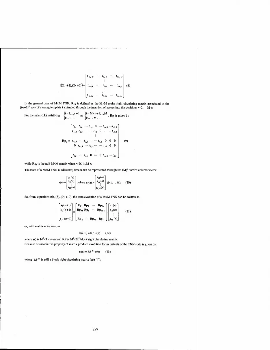
f((2r+l);(2r + l))=

'o,-r ••' (+r,-r

'-r.+.

(8)

In the general case of MxM TNN, Rpi is defined as the MxM scalar right circulating matrix associated to the (i-r+l)'h row of cloning template t extended through the insertion of zeroes into the positions r+2,...,M-r.

For the pairs (i,k) satisfying i = l,...,r + l [i = M-r + l,...,M

k = i-l k=i-M-l

■ trk 0 •■• /.

, Rpi is given by

-r,k '"'-U

-2,k U 'o,* 'r,* " '•

RP,= l-rjc - hjc 'r,k 0 0 0 (9)

0 l-r,k - h,k tr,k 0 0

h,k • •' lr,k 0 • • • 0 t_r t ■ ■ ■ tot

while Rpi is the null MxM matrix when r+2< i <M-r.

The state of a MxM TNN at (discrete) time n can be represented through the (M)2 entries column vector

s(«) =

s,(n) s2(«)

SM(")

where s;(rt) =

Si,l(")

Si,2(«)

si,M(")

0=1,..., M); (10)

So, from equations (6), (8), (9), (10), the state evolution of a MxM TNN can be written as

"s,(«+l)'

s2(« + l) =

_SM(« + 1)_

Rpi RP2 Rp«

Rp« »Pi •■ Rpw-i

RP2 - RPM RPl

s,(«)

s2(n) (U)

or, with matrix notations, as

s(n + l) = RP-s(n) (12)

where s() is M^l vector and RP is M2xM2 block right circulating matrix.

Because of associative property of matrix product, evolution for m instants of the TNN state is given by:

s(m) = RPms(0) (13)

where RPm is still a block right circulating matrix (see [4]).

297

4. TNN Exact and Heuristic Learning

Let us consider a pair <I.O> of input-output (M x M) images describing the desired elaboration; the initial state sx,y(0) is set to the value of pixel I(x,y) and the desired output after m steps is obtained as yxy(m)=0(x,y) (1 <x,y<M). From equations (7) and (13), we have

y„ y(m) = 0(x,y) iff sx y(m) >x y 0 sx y(0) (14)

where

fe ifO(x,y)=l *'° \< ifO(x,y)=-l (15).

sxy(m) >x y0 sXiY(0) means that final state must be greater or equal (smaller) than sxy(0) when the (x,y) pixel

of the output image 0 is equal to 1 (-1).

From equations (6), (8), (9), (10), (11), (13), the set of M2 inequalities sxy(m)>Xy0 sxy(0) (x,y=l,..,M)

contained in (14) can be written, for the case m=l, as in the following:

k=l,M2

*,y.o^My)«>)] *='.-• M;y=i M (16)

Each of the previous M inequalities represents an open half space in the CT space (the inequality unknowns, i.e. the CT weights, are contained in the RPjj terms, eq. (9)). Since (16) is the intersection of M2 Half Spaces, it represents a polyhedron (see eq. (1)). Each point in the polyhedron is a CT implementing the desired <I,0> transformation. The exact learning algorithm, based on polyhedral operations contained in the Polyhedral Library [10], is described in [4].

Whenever the CT which exactly transforms I into O cannot be found through polyhedral operations because the desired elaboration cannot be implemented (this can happen, for instance, if some contradictory information is contained in the training example), TNN can be trained through heuristic algorithms to find a CT which approximates the desired elaboration. In [4] and [5] we studied the using of the Simulated Annealing (SA) algorithm [8]. Since TNN evolve their state for very few steps (typically m values range from 1 to 3), the SA algorithm is very fast (times on a Pentium II machine are in the order of few (~5) minutes).

Once specified <I,0>, the CT radius r and the number of time steps m are chosen according to problem locality, as discussed in [4]. Using these values, SA algorithm is applied to search for the CT" which gives the best approximation of the desired elaboration. Indicating with Y(I,CT,m) the output of a TNN with cloning template CT, initial state I and m time steps of evolution, the SA algorithm is used to (nearly) solve the following minimization problem:

lb - Y(LCT*, m| = minfo - Y(l,CT, (17)

5. TNN Parallel Implementation

In order to implement on a parallel system eq. (6) and (7), we refer to a bi-imensional toroidal parallel machine with p2=pxp processors (this topology can eventually be easily embedded onto existing parallel systems).

Given a MxM image, it is partitioned into p2 subimages with size —x— (for the sake of simplicity we assume P P

M to be an integer multiple of p). In order to avoid communication during the computations, rxm additional

298

M border cells are added at each border (see fig. 1). Each processor contains — columns of the image (i.e. the

P subimage assigned to it) plus the last rxm columns of the subimage in the processor at its left and the first rxm columns of the subimage in the processor at its right (the same for the processors in the up/down directions); this data distribution is depicted in figure 1.

Processor P, Processor P, rxm columns Processor Pu

Subimage (i-1) Subimage (i) Subimage (i+1)

Fig. 1: distribution of subimages among the processors; the ilh processor has a copy of the last (rxm) columns of M

the subimage in the processor at its left, — columns of the image assigned to it and a copy of the first {rxm) P

columns of the subimage in the processor at its right

With such an image distribution, the TNN parallel algorithm is the following:

input: - CT, m, I Output:

binary image Y begin

for c=l to m do in parallel in all the processors

r ■ w M for 1=1 to —

P

forj=l to — P

compute eq. (6) enddo in parallel

endfor c do in parallel in all the processors

t ■ w M for 1=1 to —

P

for j=l to — P

compute eq. (7) enddo in parallel

end

6. Choice of the Parallel System and Comparative Results

Looking at previous algorithm, it is clear that it is synchronous, all data are accessed according to regular memory patterns and it is completely data parallel. For such reasons we have chosen the APEIOO/Quadrics SIMD massively

299

parallel system to implement TNN. Such a machine is based on pipelined VLIW custom processors which offer a peak performance of 50 Mflops. Being APEIOO/Quadrics a synchronous machine, no time must be wasted to synchronize the evolution of the computation. Thanks to the regularity of the memory access patterns, no caching policy is needed and very efficient data movement from local memory to internal register are possible, allowing very efficient (not limited by the memory data access bandwidth) computations.

The code was written using the TAO language, native for the APEIOO/Quadrics systems. With a little effort in writing efficient code (loop unrolling to avoid the pipeline stall, vectorization of memory accesses to avoid memory startup penalties) the program, tested on r=l,2,3, m=1,2,3 and M=512, showed sustained performances of 2.62 Gflops on a 128 processor system, characterized by peak performance of 6.4 Gflops and main memory of 512

, , , . , . sustained performances ,. MBytes. Defining the efficiency of the code implementation as n, = , we achieved an

peak performances

efficiency r|=0.41. As to give an idea of the high quality of this figure, we compare it to the results reported in [6], where a very similar problem (implementation of DT-CNN on massively parallel systems) was tackled. In that work the authors used a 256 processor CM-2, a 32 processor CM-5 and a 32 processor Cray T3D; all these machine have peak performances nearly equal to 4 Gflops. The best figures reported, for the best image size and CT radius, are 830 Mflops on the CM-5, 410 Mflops on the CM-2 and 95 Mflops on the Cray T3D, corresponding to T|CM-5=0.21,

T1CM-2=0-10 and r|T1D=0.024. Such efficiency figures clearly show that synchronous SIMD systems are better suited to implement TNN or DT-CNN.

Conclusion

In this work we briefly review the theory of a new class of recently introduced DT-CNN: the Toroidal Neural Networks (TNN). We have described the parallel implementation of TNN on the APEIOO/Quadrics massively parallel systems, where we achieved efficiency figures in the order of 40% with respect to the peak performances. Such high efficiency clearly show that parallel systems like the APEIOO/Quadrics are very well suited to implement TNN.

References

[1] A. Bartoloni,. et al.: A hardware implementation of theAPEIOO architecture. International Journal of Modem Physics, C4, 1993

[2] L.O. Chua, L. Yang: Cellular Neural Networks: Application. IEEE Trans, on CAS, 35, 1273-90 (1988)

[3] L.O. Chua, L. Yang: Cellular Neural Networks: Theory. IEEE Trans, on CAS, vol. 35, 1257-72 (1988)

[4] M.Coli, P.Palazzari, R.Rughi: The Toroidal Neural Networks. To appear in the Proc. of the Intern. Symp. on Circuit and Systems, ISCAS 2000.

[5] M. Coli, P.Palazzari, R.Rughi: Non Linear Image Processing through Sequences of Fast Cellular Neural Networks (FCNN). IEEE-EURASIP International Workshop on Non Linear Signal and Image Processing (NSIP^) - June 20-23, 1999, Antalya, Turkey

[6] G. Destri, P. Marcnzoni: Cellular Neural Networks as a General Massively Parallel Computational Taradigm. Int. Journal of Circuit Theory and Application vol. 24, n.3, 1996

[7] H.Harrer, A.Nossek: Discret Time Cellular Neural Networks. Int. Journal of Circuit Theory and Applications, vol. 20, Sept. 1992.

[8] S. Kirkpatrick, C. Gelatt, Jr., and M. Vecchi: Optimization by Simulated Annealing. Science, Vol. 220, No. 4598. pp. 498-516, May 1983

[9] A. Schrijver: Theory of linear and integer programming. John Wiley & Sons Ltd, 1986.

[10]D.K. Wilde: A Library for doing polyhedral operations. IRISA - Research Report n. 785 (downloadable from http://www.irisa.fr/EXTERNE/bibli/pi/pi785.html)

300

2000 6™ IEEE International Workshop on Cellular Neural Networks and Their Applications Proceedings

The Design of Cellular Neural Network with Ratio Memory for Pattern Learning and Recognition*

Chung-Yu Wu, IEEE Fellow, and Chiu-Hung Cheng

Department of Electronics Engineering and Institute of Electronics National Chiao Tung University

Engineering 4th Building, 1001 Ta-Hsueh Road, Hsing Chu, Taiwan, 300, R.O.C. TEL: 886-35-712121 ext.54215 Fax: 886-35-715412

E-mail: cvwu@alah.ee.nctu.edu.tw & p8611828@a1ab.ee.nctu.edu.tw

ABSTRACT: In this paper, the cellular neural network (CNN) with ratio memory (RM) is implemented in CMOS to recognize and classify the image patterns. In the implemented CMOS CNN, the BJT-based combined four-quadrant multiplier and two-quadrant divider with separated magnitude and sign is used to implement the Hebbien learning function and the ratio memory. Thus, the combined multiplier and divider and the CNN have simple structure and large input/output signal range. The pattern learning and recognition function of the 9x9 CNN with RM is simulated by both Matlab software and HSPICE. It has been verified that the CNN with RM has the advantages of more stored patterns for processing, and longer memory time with feature enhancement as compared to the CNN without RM.. Thus the proposed CNN with RM has great potential in the applications of neural associate memory for image processing. Keyword: Cellular Neural Network (CNN); Ratio Memory (RM); Current Mode Analog Circuit; Multiplier; Divider.

1. Introduction

It has been well recognized that the local connect structure of the cellular neural network (CNN) as introduced by Chua and Yang [1], makes it very suitable for VLSI implementation and thus enables many applications. So far, many important CNN applications have been reported. Among them, the applications of CNNs as neural associate memories for pattern learning, recognition, and association have been explored [2]-[6].

The ratio memory (RM) of Grossberg outstar structure has been incorporated in feedforward and feedback neural networks for image processing [7]-[10]. It is the aim of this paper to design the RM in CNNs for pattern learning and recognition. The new CNN with RM is simulated and analyzed. It is found that the CNN with RM has retained the advantages of RM, which is long memory time with feature enhancement. Moreover, more patterns can be recognized in the CNN with RM than those in the CNN without RM.

In Section 2, the architecture of the CNN with RM is described. The CMOS circuit design is presented in Section 3. In Section 4, both Matlab and HSPICE simulation results are demonstrated to verify the correction function of the CNN with RM. Finally, conclusion is given.

2. Architecture

The architecture of the CNN with ratio memory (RM) is shown in Fig. 1(a) where the RM is used to realize the weights of CNN among the cells. The detailed block diagram of two neighboring CNN cells with the RM is shown in Fig. 1(b). In Fig. 1(b), the block Tl is a V-I converter which is used to convert the voltage of input patterns into current. The current of input patterns is summed with the four weighted outputs from neighboring cells and converted into voltage through the resistor Rjj to form the cell state X^. The block T2d is a V-I converter with one-half absolute-value circuit and sign-detection circuit to generate the absolute value of output Current and detect the signs of X^, respectively. Both Tl and T2d form a CNN cell.

The block Mul/Div in Fig. 1(b) is a combined multiplier and divider circuit used to perform the learning function and store the resultant weight in the capacitor Czi. The block T21 transfers the absolute value of the voltage stored in Czi to Czs and stores its sign in the latch circuit. The block T3 is also a V-I converter to convert the voltage of Czs into current. The output current of T3 is sent to the sum block to perform the summing function with the currents from the three neighboring cells. The summed current is sent to the Mul/Div block for ratio-memory generation. The above circuits form the RM among CNN cells.

* This research was supported by t) e National Science Council (NSC), Taiwan, R.O.C, under the Grant NSC89- 2215-E-009-051.

0-7803-6344-2700/$10.00 ©2000 IEEE 301

cell l|i cell °*^ TH

EH^ ,£X, us cell J i | * cell J11 * EH

EH

EH

cell EH

cell EH

ratio

EH cell EH

cell EH

cell

.cell(ü). (a)

..ratio memory.. cellQcJ).

Figure 1: The block diagram of a) The CNN with ratio memory (RM); b) the detailed architecture of two neighboring cell and their ratio memory (RM).

In the proposed CNN with RM, the Hebbien learning rule is used. During the learning period, the RM configuration is shown in Fig. 2(a). In Fig. 2(a), the input patterns are read sequentially through Tl and T2d to extract their absolute values and signs. Then the input patterns of two neighboring cells are sent to the four- quadrant multiplier in the Mul/Div to generate the signed weight using their absolute values and signs. The generated weights are summed over m patterns for m patterns and stored in the capacitor Czi of the RM. The generated weight from Mul/Div at t = 0 when the learning period ends can be written as

(i) " ijkl (•)= I ['S*£)/'* « N,('5)

where x f is the pixel value of ith row and jth column of the pth pattern out of m input patterns, xR is the input

pattern from the cell (k,l) of Nr neighboring cells, lb is a constant bias current, andzz^is the weight stored in

Czi. Through T21, the absolute value of the weight ziuy denoted as ah^zinuiO)] is stored in the capacitor Czs,

whereas the sign of ziW/ is stored in the latch circuit of T21. As time elapsed, the leakage current Ifcal,,,t associated

with Czs gradually decreases afts(zi,u;(0)] of Czs. Since the leakage current is nearly constant, the change of

zsIJU(t) can be written as ™ijkl[<)= ^ijkl^)-[hmlmgelC2s)t

ratio memory ce|l(k,l) cctl(u) (?tjo memory ccllft.l)

I (2)

.ccl.l(ij).

(a) (b) Figure 2: The block diagram of the CNN with ratio memory (RM) a) in the learning period and b) in the recognizing period.

302

In the recognizing period, the architecture of RM is shown in Fig. 2(b). In Fig. 2(b), the Cell state X;.- can

be written as

where x?, in this period is the input pattern to be recognized, Yu is the cell outputs from Nr neighboring cells,

and wjßi(t) is the ratioed weight at time t. Wy/j (r) can be written as [7]-[9]

*>ijU (') = zi ijkl (0 E zs i]U (0f (4)

Note that wyja is generated by the two-quadrant divider in the block Mul/Div with its sign equal to the sign

of zip/latched in T21 whereas w,^/ (0YM m (?) generated by the four-quadrant multiplier of Mul/Div by using

the latched sign of Wijkl and the sign of Yw in T2d. The output current Iomd represents the term wtjU (t)Yu . The

absolute value |Y,-,| and the sign sign(Yy) of the CNN cell output Y,j can be expressed as

\Yu\ = \f(xij)\ =

sign(Yj,) = (5)

where /(x y) is a sigmoid function realized by the block T2d by separating its magnitude and sign.

3. Circuit description

The CMOS circuits of T2d and T21 are shown in Fig. 3 where Fig. 3(a) shows the circuits of V-I converter with the one-half absolute-value circuit. The V-I converter is a CMOS differential amplifier with source resistance to increase the linear range. The output current Iovic is sent to the one-half absolute-value circuit to generate the absolute-value current Ioabs with the unified flow direction. In Fig. 3(a), Vbvicl, Vbvic, Vbabsn, Vbabsp are constant bias voltages. The sign of the input voltage Vin is detected by the circuit of Fig. 3(b) in the block T2d whereas the sign of w^ir is detected and latched by the circuits of Fig. 3(c) in the block of T21. In the

learning period, VL is High and VR is low in Fig. 3(c). Thus the signs of-ir^ X^are detected and used to

determine the sign ofzi^in (1). In the recognition period, the sign ofzi'.^or equivalently the sign of iv,w is

latched by setting VL low and VR high. The CMOS circuits of the blocks Tl and T3 in Fig. 1(b) are the same as T2, but without the one-half absolute-value circuit.

Detector (T2d)-► VsXij/VsXkl

VsXi/VSXkl

V> ft f\ Vswijk.

Figure 3: a) The circuit of V-I converter with the one-half absolute-value circuit which realizes the block T2. The input voltage Vin ofT2 is connected to b) the detector circuit to form the block R2d or c) the latch circuit to form . the block T21.

The block Mul/Div is realized by proposed BJT-based Multiplier-Divider shown in Fig. 4(a) [11] where the natural logarithm relation between the emitter current and based-emitter voltage of a BJT is utilized to realize the combined multiplication and division function. In Fig. 4, the one-quadrant multiplication function is performed by Q, and Q3 whereas the one-quadrant division function is performed by Q2 on I2. The op amp is used to equalize the voltages VE3 and VE4. The current mirrors connected between Q,3 and Q, (Q24 and Q4) are used to

303

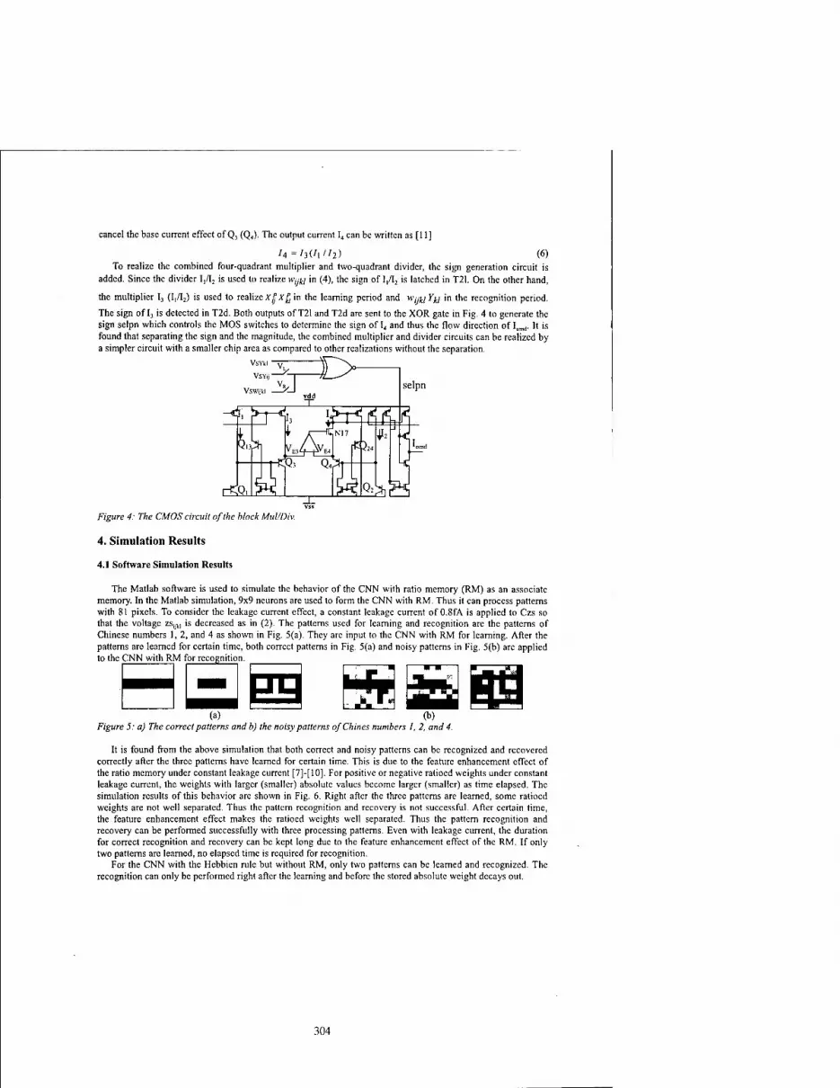
cancel the base current effect of Q, (Q4). The output current I4 can be written as [11]

/4=/3(/,//2) (6)

To realize the combined four-quadrant multiplier and two-quadrant divider, the sign generation circuit is added. Since the divider I,/I2 is used to realize wyM in (4), the sign of I,/I2 is latched in T21. On the other hand,

the multiplier I3 (I,/I2) is used to realize A-? xfi in the learning period and w„m Jy in the recognition period.

The sign of I3 is detected in T2d. Both outputs of T21 and T2d are sent to the XOR gate in Fig. 4 to generate the sign selpn which controls the MOS switches to determine the sign of lt and thus the flow direction of Ioml. It is found that separating the sign and the magnitude, the combined multiplier and divider circuits can be realized by a simpler circuit with a smaller chip area as compared to other realizations without the separation.

VSYkl "

->-n JJ^° 1 selpn

Figure 4: The CMOS circuit of the block Mul/Div

4. Simulation Results

4.1 Software Simulation Results

The Matlab software is used to simulate the behavior of the CNN with ratio memory (RM) as an associate memory. In the Matlab simulation, 9x9 neurons are used to form the CNN with RM. Thus it can process patterns with 81 pixels. To consider the leakage current effect, a constant leakage current of 0.8fA is applied to Czs so that the voltage zsijk, is decreased as in (2). The patterns used for learning and recognition are the patterns of Chinese numbers 1, 2, and 4 as shown in Fig. 5(a). They are input to the CNN with RM for learning. After the patterns are learned for certain time, both correct patterns in Fig. 5(a) and noisy patterns in Fig. 5(b) are applied to the CNN with RM for recognition.

(a) m

(b) Figure 5: a) The correct patterns and b) the noisy patterns of Chines numbers I, 2, and 4.

It is found from the above simulation that both correct and noisy patterns can be recognized and recovered correctly after the three patterns have learned for certain time. This is due to the feature enhancement effect of the ratio memory under constant leakage current [7]-[10]. For positive or negative ratioed weights under constant leakage current, the weights with larger (smaller) absolute values become larger (smaller) as time elapsed. The simulation results of this behavior are shown in Fig. 6. Right after the three patterns are learned, some ratioed weights are not well separated. Thus the pattern recognition and recovery is not successful. After certain time, the feature enhancement effect makes the ratioed weights well separated. Thus the pattern recognition and recovery can be performed successfully with three processing patterns. Even with leakage current, the duration for correct recognition and recovery can be kept long due to the feature enhancement effect of the RM. If only two patterns arc learned, no elapsed time is required for recognition.

For the CNN with the Hcbbien rule but without RM, only two patterns can be learned and recognized. The recognition can only be performed right after the learning and before the stored absolute weight decays out.

304

Tim« (min)

Figure 6: The feature enhancement effect of the ratioed weights as time elapsed.

4.2 HSPICE Simulation Results

Fig. 7 is the HSPICE simulation result of T2 which is the V-I converter with the one-half absolute-value circuit. It can be seen from Fig. 7 that the voltage Vin of the cell state X;,- is converted into positive current Ioabs.

In the range -1.5V < Vin < 1.5V, Ioabs is linearly proportional to |Vin| whereas Ioabs becomes nearly constant with Vin out of the above range. For negative Vin, the sign of Vin is detected by the circuit of Fig. 3(b) and sent out to Mul/Div.

Ioabs 15u lOu

5U O

-2 -1 Figure 7: The Hspice simulation result ofT2 circuit

Vin

From the HSPICE simulation results [ll], it is found that in the range of I, from luA to 20uA, and I3 from ljiA to 20uA with I2 kept at lOuA, the multiplication error can be kept under 5%. In the range of I, from the 1 (iA to 4|iA and I2 from 1 uA to 40 uA with I3 is kept at 4 uA, the output current can be as high as 80 uA. For the range I|<I2 which is the actual operation range, the error can be kept under 5%.

The simulated absolute weights versus time in Cell (4,4) are shown in Fig 8(a). With the large leakage current of 25nA added at the capacitor Czs to shorten the simulation time, the absolute weights are decreased quickly with time. But in the corresponding ratioed weights as shown in Fig. 8(b), the feature enhancement effect makes the larger (smaller) ratioed weights become larger (smaller) as expected.

55 us

Figure 8: a) The simulated absolute weights stored in the capacitor Czs versus time, b) The corresponding ratioed weights versus time.

In the HSPICE simulation of the 9x9 CNN with ratio memory, three Chinese number 1 2, and 4 are learned. The first recognition is performed right after learning by using the correct patterns whereas the second recognition is performed with 50|ts delay. The delay time 50|ts is required under the enlarged leakage current 25nA. Smaller leakage current leads to longer delay time. The simulated waveforms in the three cells as shown in Fig. 9.

In first recognition period of Fig. 9, the recognition errors occurs at the Cells (4,4) (4,6) (5,4) (5,6) (6,5). Since the waveforms of the Cell (4,6) is the same as that of the Cell (4,4) and the waveforms of the Cell (5,6) is the same as that of the Cell (5,4), only the waveforms of the Cells (4,4) (5,4), and (6,5) are shown in Fig. 9.

In second recognition period of Fig. 9, the ratioed weight has the feature enhancement effect to eliminate some unimportant weights. Thus the recognition can be correctly performed even with noisy input patterns. These results verify the Matlab software simulation results in Section 4.1.

305

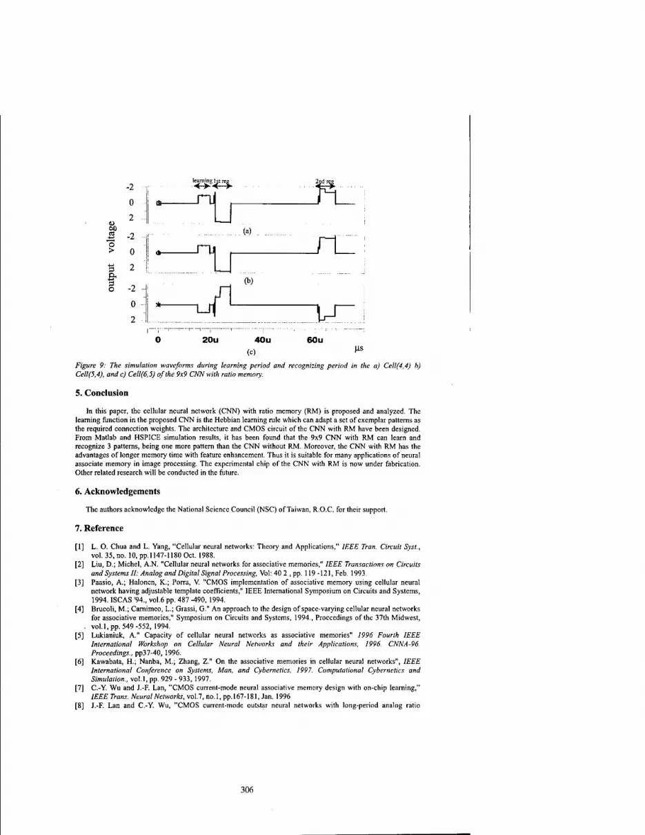
u

B >

f o

-2

0

2

-2

0

2

-2 -\

0

2

learning 1st learmng^trg^

-Til

^

(a)

(b)

2n£rM

n

M 20u 40u 60u

(c) \1S

Figure 9: The simulation waveforms during learning period and recognizing period in the a) Cell(4,4) b) Cel!(5,4), and c) Cell(6,5) of the 9x9 CNN with ratio memory.

5. Conclusion

In this paper, the cellular neural network (CNN) with ratio memory (RM) is proposed and analyzed. The learning function in the proposed CNN is the Hebbian learning rule which can adapt a set of exemplar patterns as the required connection weights. The architecture and CMOS circuit of the CNN with RM have been designed. From Matlab and HSPICE simulation results, it has been found that the 9x9 CNN with RM can learn and recognize 3 patterns, being one more pattern than the CNN without RM. Moreover, the CNN with RM has the advantages of longer memory time with feature enhancement. Thus it is suitable for many applications of neural associate memory in image processing. The experimental chip of the CNN with RM is now under fabrication. Other related research will be conducted in the future.

6. Acknowledgements

The authors acknowledge the National Science Council (NSC) of Taiwan, ROC. for their support.

7. Reference

[1] L. O. Chua and L. Yang, "Cellular neural networks: Theory and Applications," IEEE Tran. Circuit Syst., vol. 35, no. 10, pp. 1147-1180 Oct. 1988.

[2] Liu, D.; Michel, A.N. "Cellular neural networks for associative memories," IEEE Transactions on Circuits and Systems II: Analog and Digital Signal Processing, Vol: 40 2 , pp. 119-121, Feb. 1993.

[3] Paasio, A.; Halonen, K.; Porra, V. "CMOS implementation of associative memory using cellular neural network having adjustable template coefficients," IEEE International Symposium on Circuits and Systems, 1994. ISCAS '94., vol.6 pp. 487 -490, 1994.

[4] Brucoli, M.; Camimeo, L.; Grassi, G." An approach to the design of space-varying cellular neural networks for associative memories," Symposium on Circuits and Systems, 1994., Proceedings of the 37th Midwest,

. vol.1, pp. 549-552, 1994. [5] Lukianiuk, A." Capacity of cellular neural networks as associative memories" 1996 Fourth IEEE

International Workshop on Cellular Neural Networks and their Applications, 1996. CNNA-96. Proceedings., pp37-40, 1996.

[6] Kawabata, H.; Nanba, M.; Zhang, Z." On the associative memories in cellular neural networks", IEEE International Conference on Systems, Man, and Cybernetics, 1997. Computational Cybernetics and Simulation., vol.1, pp. 929 - 933, 1997.

[7] C.-Y. Wu and J.-F. Lan, "CMOS current-mode neural associative memory design with on-chip learning," IEEE Trans. Neural Networks, vol.7, no.l, pp. 167-181, Jan. 1996

[8] J.-F. Lan and C.-Y. Wu, "CMOS current-mode outstar neural networks with long-period analog ratio

306

memory," 1995 International Symp. on Circuits and Systems, Seattle, USA, vol.III, pp. 1676-1679, Apr. 29- May3 1995

[9] J.-F. Lan and C.-Y. Wu, "Analog CMOS current-mode implementation of the feedforward neural network with on-chip learning and storage," 1995 IEEE International Conf. On Neural Networks, Perth, Australia , Nov.27-Dec. 1, 1995

[10] Chung-Yu Wu and Chiu-Hung Cheng, "The Design of CMOS modified Hopfield Neural Network for pattern Recognition," International Symposium on Multimedia Information Proceeding, Session O pp585- 590 Dec. 1997.

[11] Chung-Yu Wu and Chiu-Hung Cheng, " A New analog Multiplier-Divider with compact structure for CMOS Neural Network Applications," The first Asia Pacific Conference on ASICs AP-ASIC'99, Session 13.1 pp315-317, Aug. 1999.

307

2000 6™ IEEE International Workshop on Cellular Neural Networks and Their Applications Proceedings

The Impact of the Rule Structure on the Algorithm of 2D Cellular Automata Implementation

Anna Porebska

University of Mining and Metallurgy, Faculty of Electrical Engineering, Automatics, Computer Science and Electronics, al. Mickiewicza 30, 30-059 Krakow, Poland

phone: +48 (12) 617-28-18, e-mail: porebska@uci.agh.edu.pl

ABSTRACT: In case of the 2-D cellular automata the whole rule f can be considered the set of sub-functions grouped due to the number of "ones " in the neighbourhood. Such decomposition enables indication of sub-functions, which are more important for the global dynamics of the automaton then others. The cellular automata can be implemented in Cellular Neural Network (CNN). The simplest way of such implementation on the CNN Universal Machine was proposed by Cronuse and Chua. We present the modification of this method thanks to which the information about sub-functions can be saved. Due to that we are able to simplify the architecture of a CNN-UM implementing CA. Furthermore the shortage of the time of a new state evaluation is possible. The advantage of the modified CA implementation is possibility to receive the new automaton by manipulation of this part of the structure, which is connected with the sub-function.

1. Introduction

The Cellular Automata (CA) can be analysed as the infinite or finite-size greed of cells. The states of cells are changed in discrete time and take the discrete value according to the transition function (rule). The CA rules map the state of a given cell on a discrete lattice to a future state, depending on states of the neighbouring cells [1].

The rale function is a significant element, which determines behaviour of an automaton. For the 2-D automata with von Neumann neighbourhood, which are the subjects of our investigation, the whole rule/can be considered the triplet of the form fp, JQ, £). Because the separate components determine the automaton behaviour in different manner it is important to use adequate information in the method of implementation. We make the modification of the CNN Universal Machine algorithm, proposed by Cronuse and Chua [2] for the first-order cellular automata implementation, so that the information about the form (fP, fe, fR) is saved. We show how this determines the architecture of CNN Universal Machine, especially in the case of some rule symmetry. Our modification enables simplification of the implementation of cellular automata in many cases and shortens the time of a new state evaluation. Such case is shown on examples.

2. The Decomposition of Cellular Automata Rules

An automaton can reach the concrete state, oscillate between a few values or change the state in each next step in chaotic manner. The main class of CA was shown by Wolfram [3]. The dynamics presented by a cellular automaton is determined by its rule. As it is a Boolean function, it can be represented by the truth table. Separate regions of the truth table are connected with the structure of the rule. This structure can be also reflected in the peculiar notation of the rule. It is worth stressing that manipulation of only one part of the rule has the stronger impact on the dynamics of CA then change of other parts of the rule.

2.1 The 2DCellular Automata

We can describe an infinite 2-D cellular automaton as a quadruple:

A = (I?,Vg,S,f) (1)

where: S = {FALSE, TRUE} - the set of states, LxL - the lattice dimension, V0 - a neighbourhood of (i,j)th cell / - is a transition function (rule)

In this paper we analyse the case of so called von Neumann neighbourhood (Fig. 1) defined like in (2):

0-7803-6344-2/00/S10.00 ©2000 IEEE 309

Figure 1: 5-element von Neumann neighbourhood of the cell CC

(*), •- ijfor 2D CA, marked by dote line contour

Vo = f(U), OJ-i). (U+J). O-iJ). 0*1 J)] (2)

For the state of the central cell we use the CC(t) (for simplicity, only CC) notation, and for four other neighbours - the notation corresponding with geographic directions: W(t), E(t), N(l), S(t) (for simplicity, only W, E, W, 5). Thus,

/ : (CC(t),E(t),N(t),W(t),S(t))-> CC(t + /; (3)

The sequence i%t) = (CC(t), E(t), N(t), W(t), S(t)) is called a configuration. By -i3(t) we denote the configuration opposite to -6(t) e.g.: - iS(t) = (-CC(t), -E(t), -N(t), -W(t), -S(t)) We assume that the automata are homogeneous. The state TRUE is denoted "1" and the state FALSE "-1".

2.2 The rule decomposition

For the 5-element neighbourhood K0, we can divide the sequences' domain to three parts corresponding with groups P, Q, R: P: all cells in i3(t) are the same (2Z0 = {1 sequence-all "-1"} andX5={l sequence-all "1"}) Q: four of the neighbours have the same state (£i ={5 sequences - one'T'} and^4 ={5 sequence - four'T'}) R: three of the neighbours have the same state (£2 ={10 sequences - two "1"} and £3 -{10 sequences - three

"1"}) For each of them we can find the form of the rule function. The whole transition function/can be analysed as

the triplet of the form <fP, fg, fg) where fP, fg, fK , means the possible form of the rule function for three different classes of the configuration mentioned above [4].

The notation of a rule proposed above can be easily transformed to the truth table in a manner which saves the areas connected with different groups of configurations. The truth table for the automaton with the von Neumann neighbourhood is shown on Fig.2.

Figure 2: The truth table for a rule of the 2D cellular automata with von Neumann neighbourhood. Six areas (marked with different pattern or different shade) with the same number of ones £ in configuration i%t) are differentiated.

310

Areas marked with both the same pattern and the same shade represent configurations with the same number of"l". It is symbolically marked with L, i = 0,1,2,3,4,5. Bold line separates the i3(t) states (left from the line - areas £j, i = 0,1,2) from -i3(t) states (right from the line - areas Di, i =5,4,3). Brighter and darker shades differentiate opposite configurations, e.g. (-1,-1,-1,-1,1), (1,1,1,1,-1). Altogether they constitute configurations of the P, Q, R group.

Basing on that table any rule can be written in the classic form of the sum of logical products or in the form of the product of logical sums. But we are able to do it in another way - create logical expression for each sub- function^,^, fa (or even fa i = 0,1,2,3,4,5) separately. Thanks to that, in many cases we can note the sub- function in a simplified form.

Some of thefp, fQ, fR sub-rules have stronger impact on the dynamics of an automaton then others. It is shown [4] that the Q sub-function in von Neumann neighbourhood - as well as in different neighbourhoods - is essential for the evolution of an automaton state. All ofthat, make our modification.of the method proposed by Cronuse and Chua for the first-order cellular automata implementation such useful.

3. The Modified CNN Universal Machine Algorithm for the CA Implementation

The CNN Universal Machine is a cellular analogue stored-program multidimensional array computer [5]. It was introduced to use the structure of Cellular Neural Network in different applications, where the classical digital computing is either too much time consuming or it is not powerful enough. The cellular automata implementation is a good example of such an application.

The simplified architecture of CNN Universal Machine used in CA implementation contains the CNN cells as main elements of its structure. They perform the analogue transient. The state and input is hold in the Local Analogue Memory (LAM) and a binary value for each cell is stored in Local Logic Memory (LLM). The Local Logic Unite (LLU) performs arbitrary intro-cell logic functions on the contents of the LLM [2].

3.1 Cronuse and Chua implementation of CA using CNN Universal Machine

Cronuse and Chua used the fact that the transition function /is a Boolean function of the states in the neighbourhood V0. Each of neighbourhood configuration -aft) has a corresponding Boolean expression, called a miniterm, which is TRUE if and only if the neighbourhood is in that configuration. Then, the function/is written as the sum (OR) of the miniterms for which the next state is TRUE (or as the product - AND - of maxterms for which the next state is FALSE).

The miniterms are linearly separable and can be implemented by a linear threshold class CNN (with A and B templates appropriately constructed [2]). The outputs of miniterms (TEM) blocks, stored in LLM, are arguments of the OR function implemented by the LLU.

3.2 Modified implementation of cellular automata based on the decomposition of the CA rule

In our algorithm of CA implementation we base on the decomposition of the CA rule for three sub-functions (fpfgM- The information about this structure is reflected in different areas connected with Ei - see Fig.2. The rough concept of such approach to the CA implementation was presented in [6].

Each of sub-functions fp.fQ.fit is implemented separately - see Fig.3. For this aim we can use the Cronuse and Chua algorithm. In each case we apply this algorithm exclusively for the part of the rule table which is connected with appropriate group of configuration (e.g. P, Q, R - and more precisely with Xj) - see blocks P, Q, Ron Fig.3.

We show how this modified algorithm works on the example of well-known CA called LIHENS.

Examplel-LIHENS The rule can be expressed in the following manner: The CC cell will be "1" in the next step if one or four

from its 4 remaining neighbours are in the state "1". In other cases the CC cell will not change. The automaton takes "1" for 21 different configurations. The fP, fa, ft are respectively: 1-miniterm, 10-

miniterm and 10-miniterm functions. They can be implemented as shown on Fig.3. Miniterms of sub-function are implemented by CNN with appropriate A, B templates (like in Cronuse [2]).

If we write all „ones" from the true table as miniterms, our modified implementation uses the same number of TEM blocks as the original one. They are grouped according to the configuration type (P or Q or R) only. But the signal i3ft) is sent to P, Q or R block depending on the £ value. The processing of the information is conducted only in the block, which is pointed by £ (e.g. block Q for X equals 1 or equals 4). Thanks to that, we can reduce the time of the new state of the cell evaluation. If we need to change only one sub-function, we can

311

change only that part of an architecture, which is connected with it. Moreover, the limit of possible - for given sub-function - configurations makes it possible to write the sub-rule in more compact form (instead off all miniterms, we use less Boolean expressions in the logical sum).

0 5 2 3

$(t)

fzo(ty)

-W ty

P

fzs(W)

fz-m»

-w w

fn(-W)

hiWD)

-W

fzi(-m)

r w+i)

Figure.3: A flow chart of the Modified CNN Universal Machine Algorithm for implementation of the CA with transition function f= (fp.fg.fiO-

Let us return to the LIHENS example.

Example2 - The compact notation of LIHENS We can write LIHENS rule/as below:

(fp.fg.fiO = (0/1. HL CC/CC) (4)

where - appropriate expressions for configurations from Xi and Xs-i are noted before and after the slash (e.g. fBm/fzs-,(-m,i=o,i,2). Thanks to that, the simplification of LIHENS implementation is possible. Only the P block remains the same as in the Example 1. For each Q configuration^ = /, due to that Q block contains only 2 miniterms: minitermX;= 1, i= 1,4 instead of 10 different miniterms. For each of R configurations//, takes the CC value -thus, in the R block we can reduce 10 different miniterms to 2 miniterms: minitcrmXi =CC, i=2,3.

Another advantage of our modification of Cronuse algorithm is connected with different kind of symmetry in some rules. Interesting class of cellular automata presented so called "FALSE-TRUE" symmetry - all the transition function takes opposite values for configuration and its negation. Thus, we marked the separate sub- blocks connected with i3[t) and-t!f/) on Fig.3.

If the/function fulfils a condition / of/)) =-/[-i%t)), only the implementation of ß.1%1)) is necessary - see Fig.4. Due to that we can reduce the blocks/jj(-t^i)). '=3,4,5 within blocks P, Q, R ( Fig.3). In consequence, we use only half of the TEM blocks-those connected with the truth table area left from the bold line on Fig.l. The voting rules (majority rule, ANNEAL) are the classic automata rules with the " FALSE -TRUE " symmetry.

Different symmetry is observed if the/function fulfils a condition/(i?i))=./(-«W,'- 'n tms case we als0 reduce the blocks/fl(-T^0). i=3,4,5 within blocks P, Q, R , but we need to add the NOT elements into the path of-t^r) signals.

The symmetry can appear in sub-function only. In this case appropriate sub-blocks within this sub-function realisation can be reduced.

Example} - LIHENS symmetry If we look at the true table of LIHENS or at the (4) equation, we can sec that the whole/function has the

different value for i3(t) and-t^/J. But the sub-functions manifest symmetry:

312

fP wt))= -fp (-W)). fa WW =fa (-W), h W» = h (-#(0) (5)

In this case we can reduce the blocks implementing thefL1, fm, fc 5, but we need to add the NOT elements into the paths of -iS(t) signal for Si , i=l,2. We eliminate half minitenns, what additionally simplify the all architecture. The architecture for the LIHENS implementation is shown on the Fig. 5.

5 0

-% % -H) % -*(<) 6(<)

£°(0(t))

w w-

5 4 1

JS< (»(>)) fr (H))

T

#(t+l)

Figure 4: A flow chart of the Modified CNN Universal Machine Algorithm for implementation of the CA with symmetric transition functionf= (fp.fo.fit) ("FALSE-TRUE"symmetry)

6(t) % -% % -*(t) %

fzo(«(t)) = NESCCW

-4-4Ü ■2ftL-

4 1

T 6(i+D

Figure 5: A flow chart of the Modified CNN Universal Machine Algorithm for implementation of the cellular automaton LIHENS

3.2 The Game of Life

One can asks if this decomposition can be useful in the Game of Life (GofL). This automaton is particularly interesting as the universal one and the effectiveness of the method of CA implementation can be verified with respect to this automaton. Firstly, it should be stressed that the GofL is the automaton with a wider neighbourhood then the one analysed regard in the paper (9-element Moore neighbourhood). Thus, the application of this method requires extension of the number of configuration types and the number of the sub- functions to five. If we do that, we can write the GofL rule as the set of five sub-rules in which only two

313

elements will be different then (-1). Secondly, one of these sub-functions is symmetric and the second one can be written in the compact form.

There is 140 "ones" in the true table of GofL. The "mechanic" application of Cronusc method generates 140 miniterms. If we apply our method of decomposition it well be enough to implement 3 different miniterms: minitermJi = 0, i=0,1,2,5,6,7,8,9, minitermjj = 1, miniterml^ = CC.

4. Conclusions

In our method of CA implementation, which modified the one, proposed by Cronuse and Chua, we used the information about the/structure as well as information about the/symmetry. As it was shown on the examples, such decomposition of the rule enables simplification of the received architecture.

We limited our analysis to the von Neumann neighbourhood, but the same methodology can be applied to the wider neighbourhood. Especially Game of Life can be implemented in this manner in effective way.

If we want to receive new automaton we can manipulate each of sub-functions realisations separately. It is important in the context of the great impact of fg function on the dynamics of an automaton. Moreover in the simplified architecture the time required for the new cell state evaluation is reduced.

5. Acknowledgements

This work has been supported by the research grant of the University of Mining and Metallurgy.

6. References

[ 1 ] T. Toffoli, N. Margolus: "Cellular Automata Machines", MIT Press, Cambridge, Massachusetts 1987 [2] K.R. Cronuse , L.O.Chua: "The CNN Universal Machine is as universal as the Turing Machine",

Memorandum No. UCB/ERL M95/29, Electronic Research Lab. College of Engineering, University of California, Berkeley, CA94720, 1995

[3] S. Wolfram ed.: Theory and Applications of Cellular Automata, World Scientific Publishing Co Pte Ltd., Singapore, 1986

[4] A. Porebska: "The Impact of a Transition Function Form on the Patterns Generating - the Case of the Stable 2D Cellular Automata", Proceedings the 19-th Seminar on Fundamentals of Electrical Engineering and Circuit Theory (SPETO'96), Gliwice - Ustrofi, pp. 563-556, April 1996

[5] T. Roska, L.O. Chua: •'The CNN Universal Machine: an Analogic Array Computer", IEEE Transactions on Circuits and Systems - II, Vol. 40, pp. 163-173, March 1993

[6] A. Porebska: „New Formula of 2D Cellular Automata Implementation using CNN Universal Machine", Proceedings of the XXII National Conference on Circuit Theory and Electronic Networks (KKTOiUE'99), Warszawa- Stare Jab'onki, pp. 593-598, October 1999

314

2000 6™ IEEE International Workshop on Cellular Neural Networks and Their Applications Proceedings

An Analog VLSI Time-Delay Neural Network Implementation for Phoneme Recognition

E.Gatt, J.Micallef, E.Chilton 0)

Department of Microelectronics University of Malta

Msida, MSD 06 Malta

Tel: (+356) 3290 2074 Fax: (+356) 343577

Email: ei gatt@eng.um.edu.mt

(1> School of Electronic Engineering, Information Technology and Mathematics University of Surrey Guildford, GU2 7XH

United Kingdom Tel: (+44) (0) 1483 259823 Fax: (+44) (0) 1483 534139

Email: e.chilton@eim.surrev.ac.uk

ABSTRACT: The paper proposes an analog VLSI neural network chip, which can be cascaded in order to develop a time-delay neural network system for phoneme recognition. Backpropagation learning has been adopted to train the network to recognise phoneme frames extracted from the TIMIT database. A prototype chip, implemented using CMOS 2.0fjm, double metal, double poly technology is also described, together with its specifications.

1. Introduction

In recent years, interest in neural networks has seen a major resurgence, due at least in part to the prospect of compact and dense implementation of these networks in analog integrated circuit form. In fact, a number of direct analog implementations have been manufactured and these consist mainly of building blocks that are suitable for the artificial paradigms [1-3].

Analog neural network systems are preferred to their digital counterparts mainly due to the high speed that they can attain. In fact, this property has made them more suitable for implementing recurrent neural networks. However, they suffer from certain constraints, due to the effects of the various circuits nonlinearities and offset errors [4-6].

No practical system can eliminate all the effects of nonlinearities and offset errors, but the proposed architecture aims at minimising these errors allowing the neural network to operate normally under the effects of these errors.

Back propagation learning has been applied successfully in a number of signal processing techniques. ■ However, with conventional back propagation learning, offset errors arising from practical analog circuits

fatally affect learning [1,2,4,6]. These effects are minimised by splitting the learning stage into two phases. Instead of using the difference between the target and output as the error signal, the target and output values are adopted as errors to the two different phases. The weight changes for both phases are calculated and the net weight change would be obtained by subtraction [1,3,4,6].

This system provides gradient descent learning so long as the learning rate is small enough. This is possible in most systems and minimises the effects of offset errors while finding the network weights. Also, no extra memory is required and the subtraction operation between the two learning phases tends to cancel out most of the offset errors. This is possible at the expense of a slight increase in circuitry.

0-7803-6344-2/00/$10.00 ©2000 IEEE 315

Time-delay neural networks (TDNNs) have been particularly useful for phoneme recognition systems [7]. The basic unit used in many neural networks computes the weighted sum of its inputs and passes this sum through a non-linear function. In TDNNs, the basic unit is modified by introducing delays. Using this kind of architecture the TDNN unit has the ability to compare the current input to the past history of events. The sigmoid function is the preferred non-linear function that is normally adopted for each unit. The architecture adopted for phoneme recognition is a three-layer net. Each collection of TDNN units is duplicated for each one frame shift in time. In this way, the whole history of activities is available at once. Since the shifted copies of the TDNN arc mere duplicates, the weights of the corresponding connections in the time-shifted copies must be constrained to be the same. Of course, this applies to all connections and all time shifts and in this way the network is forced to discover useful acoustic features in the input, regardless of when in time they actually occurred. This is an important property, as it makes the network independent of error-prone pre-processing algorithms that otherwise would be needed for time alignment and/or segmentation. The training time can be minimised by first applying a small training set and then increasing it gradually. Back- propagation learning was adopted to train the network. One point to note is that the structure of TDNNs is very simple and is ideal for VLSI implementations due to its regular topology.

In this paper, we review the main components of a speech recognition system, including the main speech coding techniques adopted and simulation results obtained. Section 3 describes the hardware requirements of the chip, while section 4 includes a description of the performance of the implemented chip,

2. Speech Recognition Systems and Simulation Results

Figure 1 shows the components of a speech recognition system. The input to the recognition system is the physical speech signal. The speech signal must be sampled, digitally encoded and stored. The speech input is then transformed into a sequence of speech feature vectors to eliminate any redundancies. The next step is to identify patterns in the feature vectors corresponding to speech units such as words, phrases or phonemes and finally further analysis is performed on the pattern-matching results in order to arrive at the recognition decision.

A wide range of possibilities exists for paramctrically representing the speech signal. These include short time energy, zero crossing rates, level crossing rates and other related parameters. One of the most important parametric representations of speech is the short time spectral envelope. Spectral analysis methods are therefore generally considered as the core of the signal-processing front end in a speech- recognition system. The two dominant methods of spectral analysis are the filter-bank spectrum analysis model, mel-scale cepstral coefficients and the linear predictive coding (LPC) spectral analysis model.

Several simulations were carried out on time-delay neural networks in order to establish the best method of coding the speech data and also to evaluate possible network configurations. Two different architectures were tested. The first option involved a system to first classify the phoneme and then channel the data to a dedicated neural network for identification, while the second option involves feeding the speech data to a neural network for direct identification. Both systems resulted in approximately the same recognition rates and the second option was preferred since it results in an overall smaller network size. In both cases, simulations were carried out to identify an ideal network size that would give a good recognition rate, a low training time and minimal complexity so that the chip can be feasibly implemented using VLSI techniques. Table 1 illustrates the results of simulations carried out to determine the best speech coding technique for recognition purposes. For the above simulations 4000 phoneme samples were used for training the network while another 4000 samples were adopted for evaluating the performance of the network. The 4000 samples were extracted from 40 different speakers (20 male, 20 female) from different dialect regions and a 39-dimcnsional vector was computed for each coding scheme. The neural network adopted was a three- layer network having 39 input nodes, 200 hidden neurons and 48 output nodes - each output node representing a particular phoneme.

Table 2 illustrates the results of simulations carried out to determine an ideal number of hidden neurons that would give a good recognition to training time compromise. Again a three-layer neural network was adopted and the training time is mainly dependant on the number of neurons in the hidden layer. The network was fed mel-scale input vectors, together with their delta and acceleration coefficients.

316

S(N)

Speech

Analysis System

FilterBank,LPC,DFT Pattern Training

Feature Measurement T

Templates or

Models

v

Decision Logic Pattern Classifier

Local Distance Measure - Dynamic Time Warping

Figure 1: Components of a Speech Recognition System

Coding Method Overall Recognition Rate

LPC with delta and acceleration coefficients 55% PARCOR with delta and acceleration coefficients 58%

Log Area Ratios with delta and acceleration coefficients 57% Cepstral Coefficients with delta and acceleration coefficients 62%

Mel-Scale Cepstral Coefficients with delta and acceleration coefficients 66%

Table 1: Simulation Results Comparing the Different Input Speech Coding Techniques.

As can be seen from Table 2, a network having 150 neurons in the hidden layer just gives a slightly smaller value for the recognition rate than a network having 350 neurons, but would result in a much smaller silicon area and a reduction in training time.

No. of Neurons in the Hidden Layer Recognition Rate

350 67.2% 300 66.7% 200 66.2% 150 65.8% 100 59.7%

Table 2: Simulation Results showing the Recognition Rates obtained as a function of the number of neurons in the hidden layer

317

3. Hardware

The neural network is mainly composed of 3 building blocks: the neuron unit, the synapse unit and the error signal generator.

The neuron unit performs two main functions: • it transforms an input current, U to a voltage output, Out, according to a sigmoid function with

variable gain, SG. This function relates to operation of the neuron in either the hidden layer or output stage.

• it buffers an input voltage, J and this function relates to a neuron operating In the input stage.

Figure 2 shows the schematic diagram for a neuron unit. The synapse unit has two paths, one for the feed forward pass and the other for back propagating the error. As can be seen from Figure 3, which illustrates the schematic diagram of the synapse unit, it requires three multipliers and a weight-processing unit for the storage and update of weights. During the forward pass, the synapse accepts the Out signal from a neuron in the previous layer at the O terminal and it produces an output signal WO, while during the backward pass, it accepts the error signal, D, from the error-signal generator unit and produces an error signal, WD, to be propagated to the synapses in the previous layers.

SG

-> Out

Amplifier

Figure 2: Neuron Unit Schematic Diagram T

WD

Figure 3: Synapse Unit Schematic Diagram

The error signal generator unit provides an error signal by multiplying the input error, E, by the differential coefficients of the neuron activation levels. Resistors are used to convert currents to voltages and a variable gain is available to improve learning. Figure 4 shows the schematic diagram for the error signal generator unit. SG2 is the sigmoid gain of the differential coefficient. These error signals are then used to modify the

318

synaptic weights in the synapse units and at the same time, they are weighted and output from terminals WD.

U

SG2

d(Vin) dt

T T Figure 4: Error Signal Generator Schematic Diagram

3.1 Electronic Circuits Considerations

The building blocks mentioned in the above section are made up of the following circuits: amplifiers, multipliers, differentiators and weight-processing units.

The amplifier is a simple differential pair and is used as an activation function generator and a buffer with differential outputs.

Multipliers are the most important components in the neural network as they are the most commonly used block and determine the degree of integration and power consumption. The Gilbert multiplier was adopted because of its small size and low power dissipation [7].

The derivative generator is based on the fact that the derivative of the sigmoid function, /, can be obtained by shifting the square of the sigmoid function and this can easily be obtained with a slight modification to the multiplier circuit.

/'=!-/' (1)

The weight-processing unit is used to hold the weight data, output it and modify it in proportion to an error signal input. A capacitor memory is used due to its small size. Figure 5 illustrates the block diagram for the weight-processing unit circuit. The input signal to the weight-processing unit is converted to constant voltage pulses with widths proportional to the error signal. Comparing the input error signal with a triangular waveform, CMP, which has a typical frequency of 100 kHz, does this. The output of the voltage- to-pulse converter charges a capacitor to a voltage representing the weight. A control signal, PL, is also required in order for the weight-processing unit to differential between operation in the forward and the backward pass. Normally, the weights were initially set to 0.1V. This value normally allowed the weights to converge to the required value. Another aspect that must be taken into account is the weight memory leakage. In order to minimise memory leakage, the time constant is made as large as possible. This is possible by using large capacitances.

CMP

IN

Voltage To

Pulse Converter

Capacitor Charger -*• Out

Figure 5: Weight-Processing Unit Block Diagram

319

4. Circuit Evaluation

An integrated circuit, incorporating 6 neurons, 6 synapses and 6 error-signal generator units was implemented and these prototype chips were used to implement a fully interconnected three-layer time- delay neural network having 13 input nodes, 20 hidden nodes and 5 output nodes. The network was trained and tested using 50 vowel frames from 5 different speakers in order to evaluate the performance of the chip. Using the same training and testing set, the overall recognition rate was 85.3%, which was about 2.1% lower than the recognition rate obtained during simulations. This difference could be accounted for by the various nonlinearities present in analog components.

Using a supply rail of ±5V, the maximum power consumption in the synapse unit was 3mW, that of the neuron unit was lmW and the error-signal generator could consume a peak of 2mW. Also the forward propagation time was found to be approximately 5ns and a time of 25|is was found to be an appropriate learning time for each frame vector.

5. Conclusions

Using a smaller dimension CMOS process such as 0.35ujn a 5mm by 5mm chip could include up to 150 neurons, 150 synapses and 150 error-signal generator units making it possible to construct a full time-delay neural network for phoneme recognition, using just a single chip. This chip could then be interfaced to a computer to generate a fully automated phoneme recognition system.

6. References

[1] T. Morie and Y. Amemiya, "An All-Analog Expandable Neural Network LSI with On-Chip Backpropagation Learning": IEEE Journal of Solid State Circuits, Vol. 29, No. 9, pp.1086 - 1093, Sept. 94.

[2] P. Hollis and J. Paulos, "A Neural Network Learning Algorithm Tailored for VLSI Implementation": IEEE Transactions for Neural Networks, Vol. 5, No.5, pp. 784 - 791, Sept. 94.

[3] S. Satyanarayana, Y. Tsividis and H. Graf, "A Reconfigurable VLSI Neural Network": IEEE Journal of Solid State Circuits, Vol. 27, No. 1, pp. 67-81, Jan. 92.

[4] Y. Arima, K. Mashiko, K. Okada, T. Yamada, A. Maeda, H. Notani, H.Kondoh and S. Kayano, "A 336-Neuron, 28K-Synapse, Self-Learning Neural Network Chip with Branch-Neuron-Unit Architecture": IEEE Journal of Solid State Circuits, Vol. 26, No. 11, pp. 1637- 1644, Nov. 91.

[5] M. Valle, D. Caviglia and G. Bisio, "An Experimental Analog VLSI Neural Chip with On-Chip Backpropagation Learning": ", 18,h European Solid State Circuits Conference 92, pp. 203 - 206.

[6] P. Hollis and J. Paulos, "Aritificial Neural Networks Using MOS Analog Multipliers": IEEE Journal of Solid State Circuits, Vol. 25, No.3, pp.849 - 855, Jun 90.

[7] J. Delgado-Frias and W. Moore, VLSI for Neural Networks and Artificial Intelligence, Plenum Publishing 1994.

320

2000 6™ IEEE International Workshop on Cellular Neural Networks and Their Applications Proceedings

Overlapping issues in designing large CNNs

Asko Kananen, Ari Paasio, Kari Halonen

Electronic Circuit Design Laboratory, Helsinki University of Technology P.O.BOX 3000, FIN-02015 HUT, FINLAND

phone: +358-9-451 5013 fax: +358-9-451 2269 e-mail: Asko.Kananen@ecdl.hut.fi

ABSTRACT: In this paper some problems in designing large gray-scale Cellular Nonlinear Network silicon implementations are discussed. These problems effect both the processing speed of the network and the silicon area needed for the network. The presented problems are being solved by reducing the number of cell-rows. The difference between the method given here and between the previously presented solutions is the simultaneous evaluation of the output while still writing in the remaining input data. This method leads to a problem of a required overlapping in a frame. Both, the system level description of the "transient rolling" and simulation results of the overlapping problem are given in this paper.

1. Introduction

Cellular Nonlinear Networks [1] have been shown to be very effective in the field of image processing and in other computationally demanding tasks. Even though the grid size of the CNNs have been growing rapidly lately [2, 3, 4], only few of the chips [3, 5] are designed for gray-scale operations. If the operation speed is compared between [3] and the chip previously presented by the same group [6] as it was done in [7] it can be seen that the total operation speed was not increased linearly to the number of cells, actually there was hardly any gain in total processing speed when moving from 20 x 22 to 64 x 64 cell grid. Of course there are differences in functionalities but the increase in operational speed was not what it was expected. If on the other hand the grid size of the chips mentioned above is monitored, only [4] is of QCIF-size and others are smaller than any standardized image size. This leads to the fact that in order to process a whole image, the processing has to be done in parts. Different problems arise when moving to larger designs, in the sense of number of the cells, and in some cases it can be more efficient to implement only part of the network than a full-size network.

In this paper we discuss some of the problems we faced in our new design implementing a CNN low- pass image filter. First, the system requirements and problems arising from those are discussed. Then, system solution for those problems is given and some system simulation results are shown. Finally the new system is described in detail and some comparisons are made between different approaches.

2. Problems arising when implementing large networks

The goal of the study was to implement the gray-scale part of the algorithm published in [8] with such a high cell density that it would be possible to get a single-chip implementation of the video segmentation algorithm with the black-and-white network [4] and the designed gray-scale part. This implied really hard requirements for the size of the cell.

2.1 Input image memory

The input to the gray-scale part is planned to be done in a row-by-row manner from the frame memories. Since the image size in QCIF-format is 176 x 144 pixels, it means that the difference between storage times for the first row and for the last row is 144 times the clock cycle if the whole image is first loaded to the cells and then the evaluation is started. And if the results are read out in the same manner the same problem is there too.

When combining the cell size and the memory requirements we get to a point where we have to have large enough memory capacitance in each cell to store the input value before the processing can start. This same capacitance is also the input capacitance of the cell, and this effects the speed of writing in the input value. The larger the value is, the slower input clocking rate has to be used. That, in turn, increases the time the values have to be kept in the memories before the processing itself can begin. The area where the capacitance value effects the most is the size of the cell where every square micron increase

0-7803-6344-2/00/$10.00 ©2000 IEEE 321

of the size of the capacitance is multiplied by 25344 in the case of the full cell grid. The solution for the trade-off between these capacitance value requirements was not easily found so a method was developed where the starting of the processing and the reading out of converged values are done while still writing the input values to other parts of the network. In this way we were able to reduce the storage time for the pixel values and in that way smaller memory capacitances were needed. Since all the cells are not 'active' all the time there was no point in implementing a 144 x 176 network. The size of the network was also a compromise. This time the compromise had to be done between silicon area and computational efficiency. This is discussed in a later chapter.

The method of image portioning has been used mainly because the achieved cell size has been so large that any standardized frame size would result in a very large chip. Previously the network has been moved around the processed frame with some overlap in order to get the whole frame processed. In our approach we reduced the number of cell rows but kept a full width of the image. With row-by-row input to the network we are able to "roll" the evaluation over the frame and simultaneously evaluate the output while writing the input to proceeding cell rows. This method reduces the time used for the evaluation of the whole frame compared to the previously used method where normally a square shaped sub-images have been considered.

When reduction of the grid size is applied, one big problem is how to maintain the neighborhood for each cell similar to the full-size grid neighborhood and how to achieve the same or close enough accuracy. This is, of course, dependent on the used template set. If only B-templates are used, only the nearest neighbors are needed to maintain the accuracy but if the contribution of the pixel is spreading to a larger neighborhood, that is non-zero non-center values in A-template are used, the required overlapping is case dependent. This has not been discussed widely in the CNN literature. In this paper the overlapping requirement is evaluated only for the templates used in our chip. The simulation for the overlap evaluation is discussed in the following section.

3. System simulations

There were two template sets used in the gray-scale part; one with only B-template and another with A- and B-templates. For the first set the solution for the needed neighborhood is easy, as mentioned above, only nearest neighbors are needed. But for the second template set the answer is not that simple, due to this propagative nature of the set. Template for the latter case is given in equation 1.

0 1 0 0.1 0.1 0.1 1 -4 1 B = 0.1 0.2 0.1 0 1 0 0.1 0.1 0.1

7 = 0 (1)

In the design of the low-pass filter network the goal was set to achieve five to six bits accuracy. This meant that the systematic error which is caused by limited overlapping neighborhood of a cell row should be smaller than the error tolerance of the whole system.

Since it was chosen in the beginning of the design flow that the input to the network is fed in a row-by-row manner, the width of the implemented circuit was a full 176 cells and only the number of cell-rows in vertical direction effects the systematic error. In the simulations the used network size was 20x4 and the results were obtained simply by monitoring the outputs of the cell-row in the middle of the network and by chancing the number of active cell-rows, i.e. the cell-rows where the output of a cell is affected by currents coming from the neighbors and from the cell itself.

In the simulations the network consisted of resistors. As it was shown in [9] resistive networks are a special case of CNNs and the templates in equation 1 can be considered as a resistive network. This approach was taken for simpler simulation network and for getting a theoretically better answer for our problem.

In table 3. the results from our simulations are shown. The input figure was varied and the reference result was taken from a network of size 4 x 20. From the results it can be seen that this template set needs at least five neighboring cell rows to keep the accuracy in the required level. A matter left to decide was the size of the implementable network. The results from the simulations required at least five border cells on both sides of the active cell rows, i.e. the cell rows where the results were read from. It was estimated that 24 active cell rows was enough for our purposes. One reason for this was simply that 144 is dividable by 24, which in turn means that a cyclic controlling could be used, and special control signals were only needed for the beginning and for the ending of the image. The other reason was that we were able to maintain most of the computing power, as it will be shown in the next section. In the following section also the functionality of the system is described in more detail.

322

OVERLAP PIXELS

ERROR %

0 137 1 56 2 22 3 8 4 3.3 5 1.2 6 0.5

Table 1: Effect of limited overlap to the processing error

4. Evaluation flow of the system

The system described here consists of 34 identical cell rows and of border cells to realize the zero-flux border condition.

The processing starts with writing to the first eleven rows of the low-pass circuitry. The first five rows now act as border cells and they all get the same input value, i.e. the value of the first row of the image. Also, the first active row, namely the sixth one, gets the same input. Then the row by row image loading continues normally until at the same time as the writing to the twelveth row takes place, the transient for the first eleven rows is started and the evaluation begins for these rows. In the next writing cycle the transient is started also for the twelfth row. Then, when the writing to the cells is in the 14th row, the transient is on for the cell rows from one to thirteen. Now, the changes in the 14th row do not considerably disturb the already stabilized results in rows 6, 7 and 8. Therefore, the outputs of the cell rows 6, 7 and 8 can be read to the next stage, described in [10]. In the next cycle, when the input image is written to the 15th row the transient is on for the rows from 2 to 14 and the values of the rows 7, 8 and 9 are written to the next block. In this manner the evaluation continues until row 32 is reached in writing. At that stage the transient is on for the rows from 19 to 31 and the results are read from the rows 24 to 26. After this, the transient continues to be on for the rows from 19 up until the evaluation results are read from the 29th row. After this stage the converged results from rows 25 to 29 are written to the first five rows of the structure. When the values are read to the fifth row the writing continues, now from the 25th row of the original image and to the sixth row of the processor array. In this manner we have a situation where every cell has all the time at least five active cells in the vertical direction. Thus, from the 34 cell rows the first five and the last five act as border cells and the 24 rows in the middle create the low-pass filtered output. The block diagram of the low-pass part is shown in Fig.l.

CLK, // 176

I/O control

CLK,

Fixed template gray scale processor

/'

TRAN control

176

Figure 1: Low-pass ßter block diagram.

In Fig.l the TRAN control block controls which cell rows are active and the I/O-block controls the writing in and reading out to and from the low-pass block. In comparison with a full 176 x 144 network, writing and reading the results of one image takes 200 clock cycles with our approach compared to 147 cycles for the full size network (144 for writing, 2 for settling and one for reading). Here we assume that in the full size network the circuitry for the next processing stage is located inside the same cell as the low-pass structure so that the results of the network can be read out simultaneously. If this is not the case, then 144 cycles instead of one are required for row by row reading out of the result and the total evaluation speed of this task becomes worse for the full sized network compared to our approach. This is due to the well known I/O bottleneck of parallel processor

323

structures. From the above discussion it can be concluded that it is the nature of the input and output image loading that allows'us to effectively use a smaller network to process a large image and still to maintain almost the same processing speed. This fact is also discussed e.g. in [11]. With the used 10MHz clock, 200 cycles results in an evaluation time 0.02ms per image, fast enough for the input image rate of 30 figs/s. In addition to savings in the number of cells this approach also reduces the size of one cell since the required storage time for the pixel value is reduced from the 144 clock cycles to 13 clock cycles and allows smaller capacitance value for the memory capacitance. This in turn reduces the time constant in writing the input data.

5. Conclusions

In this paper some of the problems faced when implementing large CNN networks were discussed and then a system level solution for these was presented. This solution is based on rolling the image over the network and simultaneously writing in the input and reading out the processed output. That lead to a another problem, the needed neighboring cell rows to maintain the accuracy of the computation. To solve this problem, a simulation system was described and the results concerning this were shown. Also a more detailed description of the rolling system was given.

Acknowledgments

This work is supported by the Academy of Finland (#1168301/00) and (#1366361/99). The work of Asko Kananen is also suppoported by the Finnish Cultural Foundation, the Nokia Foundation and the EIS Foundation.

References

[1] L.O.Chua and L.Yang, 'Cellular Neural Networks: Theory', IEEE Transactions on Circuits and Systems, Vol. 35, pp.1257-1272,1988

[2] A.Paasio, A.Dawidziuk, K.Halonen, V.Porra, 'Minimum Size 0.5 Micron CMOS Programmable 48 by 48 CNN Test Chip', European Conference on Circuit Theory & Design, Budapest, pp.154 156, 1997.

[3] GXinan, P.Foldesy, A.Rodriguez-Vazquez, S.Espejo, R.Dominguez-Castro, E.Roca, 'A 0.5 fim CMOS 106 Transistors Analog Programmable Array Processor for Real-Time Image Processing', European Solid State Circuits Conference, ESSC1RC99, Duisburg, pp.358-361,1999.

[4] A.Paasio, A.Kananen, K.Halonen, V.Porra, 'A QCIF Resolution Binary I/O CNN-UM Chip', Jour- nal of VLSI Signal Processing, Vol. 23, pp. 281-290, 1999.

[5] P.Kinget, M.Steyaert, 'Analog VLSI Integration of Massive Parallel Processing Systems', Kluwer Academic Publishers, Dordrecht, The Netherlands, 228 pages, 1997.

[6] S.Espejo, A.Rodriguez-Vazquez, R.A.Carmona, P.Foldesy, A.Zarandy, P.Szolgay, T.Sziranyi, T.Roska, '0.8 um CMOS Two Dimensional programmable Mixed-Signal Focal-Plane Array Proces- sor with On-Chip Binary Imaging and Instruction Storage', IEEE Journal on Solid State Circuits, Vol.32, pp.1013-1026,1997.

[7] A.Rodriguez-Vazquez, E.Roca, M.Delgado-Restituto, S.Espejo and R.Dominguez-Castro, 'Most- Based Design and Scaling of Synaptic Interconnections in VLSI Analog Array Processing CNN Chips', Journal of VLSI Signal Processing, Vol. 23, pp.239-266, 1999.

[8] A.Stoffels, T.Roska, L.O.Chua, 'Object-Oriented Image Analysis for Very-Low-Bitrate Video-Coding Systems Using the CNN Universal Machine', International Journal of Circuit Theory and Applica- tions, Vol.25, pp.235-258,1997.

[9] B.E.Chi and L.O.Chua, 'Resistive Grid Image filtering: Input/Output analysis via the CNN Frame- work', IEEE Transactions on Circuits and Systems, Vol. 39, pp.531-548, 1992

[10] A.Paasio, K.Halonen, 'Cellular Nonlinear Network Implementation for Nonlinear B-Template', Pro- ceedings of CNNA 2000, Catania, Italy.

324

[11] G.Han, J.Pineda de Gyvez, E.Sanchez-Sinencio, 'Optimal Manufacturable CNN Array Size for Time Multiplexing Schemes', International Workshop on Cellular Neural Networks and Their Applications, Seville, pp.387-392,1996.

325

2000 6™ IEEE International Workshop on Cellular Neural Networks and Their Applications Proceedings

Automatic CNN Multi-Template Tree Generation.

V. M. Preciado, D. Guinea, J. Vicente, M. C. Garcia-Alegre and A. Ribeiro.

Institute de Automatica Industrial- Spanish Council for Scientific Research La Poveda (Arganda del Rey) - 28500 Madrid, Spain, preciado@iai.csic.es

ABSTRACT: A fruitful field into the CNN research domain is being the development of analogic algorithms that combine single templates to perform complex image processing. The results would be extremely useful for pattern recognition in industrial and robotic applications. This work presents a general methodology for the automatic generation of analogic algorithms by means of a genetic search. A genetic algorithm for generating multi-template trees, concept derived from the AI field, is applied to the automatic generation of analogic algorithms, based in both genetic- evolutionary search and heuristic approaches.

1. Introduction

The traditional image processing techniques require a lot of computational effort as pixel information is acquire and processed sequentially and data flow trough an A/D conversion stage. This generates a time delay that is unacceptable for real time image processing in visual tasks requiring the process of several millions of pixels per second (e.g. automatic industrial inspection, visual based navigation in robotics).

A massively parallel architecture that works with analog signals could offer a solution for these applications. This is just the basis idea of Cellular Neural Network (CNN's): an array of analogic dynamic processors whose cells interact directly within a finite local neighborhood [1], The local CNN connectivity allows its implementation as VLSI chips that can operate at a very high speed, with a high complexity level [2]. Nowadays CNN architectures implemented as VLSI chips shows the aptitude of extremely high speed compared with traditional digital image processing tools. The proliferation of ever more sophisticated CNN architectures, and the great effort observed during last years- to implant practical system based on CNN chips, drives the development of analog algorithms able to perform complex image processing tasks required in industrial applications [3], robotic systems, classification [4], and compression [5].

The objective of this work is the generation of a learning machine within the CNN paradigm, capable of finding solutions for complex image processing tasks. First a general machine for automatic analog algorithm design independent of the problem to solve is proposed. It uses an evolutionary strategy that is an extension of the genetic programming [6]. Second, this work introduces a set of sub-mechanisms to increase the power of the genetic programming and to reduce the enormous search space to optimise time. Some concepts are related with AI theory, in such a way that the performed work is at the intersection of AI, Image Processing, and CNNs fields.

Previous works present some CNN simulators with the feature of the automation of single template generation [7][8]. In this line our former work [9] describes an example-based learning method using a Genetic Algorithm for automatic generation of a single template. Current work gives flexibility to former approach proposing a method for the automatic generation of a template sequence instead of a single template GA based.

2. Multi-Template Tree Representation

The main objective of this work is the automatic generation of an adequate template sequence to transform an input image into an output image, using an initial state. This template sequence can be represented by means of a tree formed by templates, namely multi-template tree, Figure 1.

The notation utilized to codify the multitemplate tree , in a way useful for our automatic GA searching, is the prefix or Polish notation due to Lukasiewicz. According to this notation an operator O which performs an action on two objects x and y is represented Oxy. In our case, O consist of a single template, x is an input image and y is the initial state for the CNN differential equation to be solved. No parenthesis are needed and the principle operator for any term appear at the head of that term.

0-7803-6344-2/00/$10.00 ©2000 IEEE 327

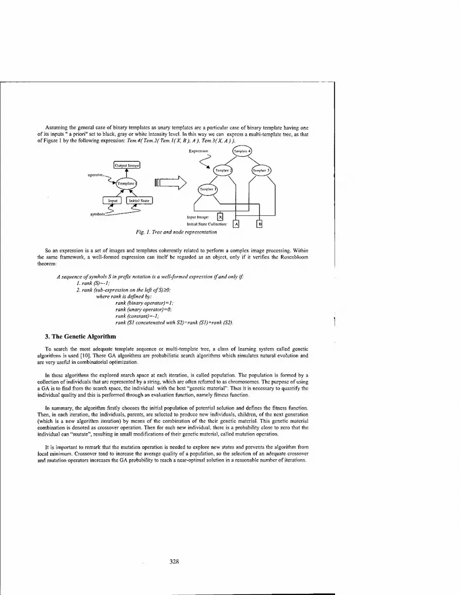
Assuming the general case of binary templates as unary templates are a particular case of binary template having one of its inputs " a priori" set to black, gray or white intensity level. In this way we can express a multi-template tree, as that ofFigure 1 by the following expression: Tern.4( Tem.2( Tern. 1 (X, B ), A), Tem.3(X, A) ).

Expression

symbols

[ Input J | Initial State j

s Input Image:

Initial State Collection: IA] [ B|

Fig. 1. Tree and node representation

So an expression is a set of images and templates coherently related to perform a complex image processing. Within the same framework, a well-formed expression can itself be regarded as an object, only if it verifies the Rosenbloom theorem:

A sequence of symbols S in prefix notation is a well-formed expression if and only if 1. rank (S)=-l; 2. rank (sub-expression on the left ofS)>0;

where rank is defined by: rank (binary operator)=l; rank (unary operator)=0; rank (constant)^-]; rank (SI concatenated with S2)=rank (Sl)+rank (S2).

3. The Genetic Algorithm

To search the most adequate template sequence or multi-template tree, a class of learning system called genetic algorithms is used [10]. These GA algorithms are probabilistic search algorithms which simulates natural evolution and are very useful in combinatorial optimization.

In these algorithms the explored search space at each iteration, is called population. The population is formed by a collection of individuals that are represented by a string, which arc often referred to as chromosomes. The purpose of using a GA is to find from the search space, the individual with the best "genetic material". Thus it is necessary to quantify the individual quality and this is performed through an evaluation function, namely fitness function.

In summary, the algorithm firstly chooses the initial population of potential solution and defines the fitness function. Then, in each iteration, the individuals, parents, are selected to produce new individuals, children, of the next generation (which is a new algorithm iteration) by means of the combination of the their genetic material. This genetic material combination is denoted as crossover operation. Then for each new individual, there is a probability close to zero that the individual can "mutate", resulting in small modifications of their genetic material, called mutation operation.

It is important to remark that the mutation operation is needed to explore new states and prevents the algorithm from local minimum. Crossover tend to increase the average quality of a population, so the selection of an adequate crossover and mutation operators increases the GA probability to reach a near-optimal solution in a reasonable number of iterations.

328

3.1. Individual Representation and Initial Population

In the proposed method, each individual codifies a multi-templates tree as a string in Polish notation. The initial random population and the offspring produced by each genetic operation must be a "well-formed expression" , verifying the Rosenbloom theorem. Although the individuals are strings in Polish notation, to simplify the following dissertation, a tree representation for each individual is assumed.

Therefore, the way to generate an individual is accomplished by fixing an upper and lower number of possible operations, to be carried on. The probability for a node to be either an operator or an image is given by a probability value Po for a binary operation and Pi=l-Po for an image. Following this pattern, we add new nodes taking into account the former probabilities and testing whether or not the upper and lower operation number are exceeded. The individual lenght is variable, consequently the initial population generation is performed through a list that links new term based upon the probability previously set by the user.

3.2 The Fitness Function

The fitness function is an energy function proportional to the to the difference between pixels from the current output image (Icmrm) and the desired output image (/O„I«J). For each individual t, the fitness function is expressed as,

J\t) 2^\ Desired * Current Ml which has to be minimized in the GA search process.

3.3. Genetic operators

' The GA operators, crossover and mutation can be defined as follows, Figure 2:

Crossover operator. A crossover point is randomly chosen in the first and second parent Then the subtree rooted at the crossover point of the first parent is eliminated and replaced by the subtree coming from the second parent. Crossover is the predominant operation and in our proposal it acts with a high probability about 0.85-0.90.

Mutation: The mutation operation used is the one defined by Koza [6]. The individual is probabilistically selected from the population and a point is randomly chosen, then the subtree rooted at that point is erased, and a new subtree is generated using the same random growing process used to originate the initial population. This mutation operation is performed sparingly. The probability of the mutation is 0.01, at each iteration.

Fig.2. Mutation and Crossover operators.

329

4. Search Space Size and its Prune by means of Heuristic Methods

Under the hypothesis of binary templates we can affirm that in a tree formed by S templates there are S+l free branches that can be filled by other terms (in general other trees). It can be demonstrated, as far as the initial root of a tree is an binary template, Figure 3a, and the growth process is performed by adding new templates located in each of these branches, Figure 3b and 3c. Each new template erases one of these free branches and produce two new ones. Accordingly, for each new template, a new branch appears and the initial difference between templates and branches remains the same. Beyond that, any tree of S templates can produce S+l trees by adding one new operator, so the number of possible tree with S operators is a factorial function of S, S!.

r o Q O dM \ Q

y Representation) \^^y __/

* 1// \ ^

\

I Initial State j | Input |

/ \ BRANCHES

a) One operator

6'" 1 c5~x /_b &k

/ \ / \

m v. / \ b) Two operators

c) Three operators posibilities

Fig. 3 The tree growing process

Assuming that the number of possible templates extracted from a template library, is N then the search space dimension is equal to the number of possible variations of S elements taken N by N. So, for a tree formed by S nodes the search space has Ns elements. Therefore, the search space size obtained by the set of all possible trees built with S operators, will be N5 S! . Finally, if the set of all possible trees are confined between a lower and an upper number of possible operations, SL and Su, then the number of elements in the search space would be:

IsiZEtZX, = f>s ■5!

s=sL

As previously stated, a new tree is created by adding elements in a string which represents the tree in Polish notation, taking into account the Rosenbloom's theorem to validate the tree syntax. According to former premises, a tree formed by S templates is represented by a string that includes S templates and S+l input images. The probability of a tree of S binary operators is equal to the probability to obtain the before mentionned, that is Pos- (1-Pof*1.

The influence that Po has in the probability that the tree size would be S, is displayed in Figure 4, being S the number of operations in the tree, and P(po,S) the probability of generating a tree of S operations conditioned to a Po value equal to po. The graphic shows that as far as Po grows, the function P(po,S) decreases for lower values of S and increases for the higher values of S. This implies higher probability values for big trees as po increases.. This bias becomes critic when po tends to 1, then P(l ,S) is equal to one for S=°° and zero otherwise.

A straightforward heuristic to shrink the space search size deals with the reduction of the number N of elements in the template library, thus the 88 templates have been grouped in 19 sets of elements having similar behavior. The space search size is reduced if we only take into account a resentative from each set. Then an initial search is accomplished in the reduced search space to perform later on a refinement process wherein the quality of each one of the components of the selected sets can be tested to find the most adequate multi-template tree.

330

\ ' 1 1 1

\ ' \ \

\, " \ -V • v _ v.. --. ■,

\x v \

,-V^; -. _

1 Trr— --^IZimm ~:::;^ 4 5 1.5 2

Fig. 4. Influence ofPo in the tree size.

2.5 3 S

A second heuristic, also to reduce the search space size includes an operation hierarchy in the random generation and mutation of the trees. It performs a template classification in three categories: a) Grey to Grey, b) Grey to Binary and c) Binary to Binary. Hence, all trees start from a Grey to Grey root, and when a Grey to Binary or Binary to Binary template appears, the subtree growing from this node is exclusively fashioned by Binary to Binary templates. So, the grey scale operations are isolated from binary ones being the grey to binary templates the interface between them.

5. Conclusions and Further Research

Up to now, the template design has been usually focused as an extrapolation of traditional image processing methods, and only recently complex mathematical techniques as morphology and PDE related methods, have been proposed. But in each case the success of the algorithm strongly depends on the designer expertise.

Thus, the automatic algorithm generation by GAs, here proposed, offers a new methodology to obtain an adequate sequence of operations, independently of the human subjectivy, for the development of analogic algorithm to solve general vision tasks. One of the aims of current work is to introduce this methodology for the design of CNNs algorithms in general industrial applications.

Futher research will be devoted to the automatic generation of analogic programs, taking as a model computer programs with all the diversity and complexity that they convey. In other words, programs usually contain subroutines (also called automatically defined functions, ADFs, or function-defining branches), iterations (automatically defined iterations or ADIs), loops (automatically defined loops or ADLs), recursions (automatically defined recursions or ADRs), and memory of different dimensionality and size (automatically defined stores or ADSs).

6. Acknowledgements

Present work was fully supported by Research Grants. CAM-06G-038-96: "Automation based on an artificial system at the poultry industry", CICYT 96-1392-C02-01: "Integrated active vision system", E.U. Thematic Network: "Networked industrial design and control applications using genetic algorithms and evolution strategies: INGENET", BRRT-CT97- 5034.

REFERENCES

[1] L. O. Chua, L. Yang. "Cellular Neural Networks: Theory". IEEE Trans, on Circuits and Systems. Vol. 35, No. 10. pp. 1257-1272. October 1988.

[2] S. Espejo, R. Carmona, R. Dominguez-Castro, A. Rodriguez-Vazquez, "A VLSI oriented continuous-time CNN model", Int. Journ. Of Circuit Theory and Applications, vol. 24, pp. 341-356,1996.

331

[3]P.Szolgay, I.Kispal and T.Kozek, "An Experimental System for Optical Detection of Layout Errors of Printed Circuits Boards Using Learned CNN Templates", Proceedings of the International Workshop on Cellular Neural Networks and their Applications (CNNA-92), pp. 203-209, Munich, 1992.

[4] T.Sziranyi and M.Csapodi, "Texture classification and Segmentation by Cellular Neural Network using Genetic Learning", Computer Vision and Image Understanding, Vol. 71, No. 3, pp. 255-270, September 1998.

[5]P.L.Venetianer, F.Werblin, T.Roska and L.O.Chua, "Analogic CNN Algorithms for some Image Compression and Restoration Tasks", IEEE Transactions on Circuits and Systems, Vol. 42, No. 5, 1995.

[6] J. R. Koza: "Detailed Description of Genetic Programming". Genetic Programming: On the Programming of Computers by Means of Natural Selection, MIT Press, 1992.

[7] R. Caponetto, M. Lavorgna, A. Martinez and L. Occhipinti, "Cellular Neural Network Simulator for Image Processing Applications", 1998 Fifth IEEE International Workshop on Cellular Neural Network and Their Applications Proceedings, pp.360-365. April 1998.

[8] Martin Hanggi and George S. Mostchytz, "Stochastic and Hybrid Approaches Toward Robust Templates", 1998 Fifth IEEE International Workshop on Cellular Neural Network and Their Applications Proceedings, pp.366-371. April 1998.

[9] V. Preciado, D. Guinea, J. Vicente, M.C.Garcia-Alegre and A.Ribciro, "CNN's design by GA's", European Congress on Computational Methods in Applied Sciences and Engineering Proceedings, ECCOMAS2000, Sept. 2000. Barcelona.

332

2000 6™ IEEE International Workshop on Cellular Neural Networks and Their Applications Proceedings

VLSI Implementation of a Double-Layer Single Cell RD-CNN for Motion Control

M. Branciforte**, G. Giustolisi*, V. Nicotra**, G. Palumbo*

*DEES - Universita di Catania V.le A. Doria, 6 - Catania - Italy

Phone +39 95-738-2313 - Fax +39 95-330-793 ggiustolisi@dees.unict.it, gpalumbo@dees.unict.it

**STMicroelectronics - Catania Site Stradale Primosole, 50 - Catania - Italy

Phone +39 95-740-7471 - Fax +39 95-740-7432 marco.branciforte@st.com, vincenzo.nicotra@st.com

ABSTRACT: In this paper a solution for a VLSI implementation of a double-layer single cell RD-CNN for motion control is presented. Particular attention is focused on the realisation of both the non-linearity block and the resistor implemented by means of the same transconductor in order to minimise the tolerance variations. Moreover, two solutions are given to obtain very large time constants due to the very low frequency involved in motion control. The approaches are validated by simulating both of them with ELDO and by comparing the results with a Matlab simulation.

1. Introduction

CNNs are arrays of non-linear and simple computing elements characterised by local interconnections between cells [1]. Due to their structure and their natural parallel computation ability, CNNs have been used for real-time image processing [2] and for emulating complex phenomena like chaos [3-4] or Partial Differential Equation (PDE) systems [5]. A particular class of PDEs, called Reaction-Diffusion PDEs, can be emulated by a two-layer CNN called Reaction-Diffusion CNN or simply RD-CNN. This PDE system is able to well describe some complex and natural phenomena, such as pattern formation or autonomous wave propagation, which are present, for example, in nervous tissues of some biological structures.

The literature reports some discrete electronic implementations of RD-CNNs emulating the above phenomena that were used to control a robot movement [6-7]. More specifically, a RD-CNN was realised for driving robot actuators by means of a wave propagation phenomenon in the same way as the wave propagation in nervous tissues does in small biological structures.

The purpose of this work is to draw out a feasibility study about a VLSI implementation of a motion control RD-CNN. In this application, the RD-CNN cell must reproduce much slower dynamics with respect to an image processing CNN, despite the similar single cell structure. In fact, an image processing CNN is required to have high-speed performances and to compute in a real-time fashion. On the other hand, in order to drive robot actuators properly, a motion control RD-CNN is required to elaborate very slow dynamics. This appears to be a strong limitation because of the small time-constant values that can be integrated in a VLSI implementation.

In this paper, a VLSI realisation of a double-layer single cell RD-CNN for motion control is presented. In particular, two different approaches to overcome the time-constant drawback are pointed out.

2. Model Description

The generic RD-PDE system that reproduces the phenomena described in the introduction can be written as:

(la)

—^-=~h.i.j +(l+M-e)y2W +s2yw +Dz(y2MJ +ywtlJ +yÖJ_, + y2ilJ+, -4y2„J+/2 (lb)

■=—JL. . +M + //—piv... +s.v... +/A1V.... +v.... +v-... + v-... — av.. .1+/. dt

yw=0.5kw + l|-L,.,-l|) ÜC)

0-7803-6344-2/00/S10.00 ©2000 IEEE 333

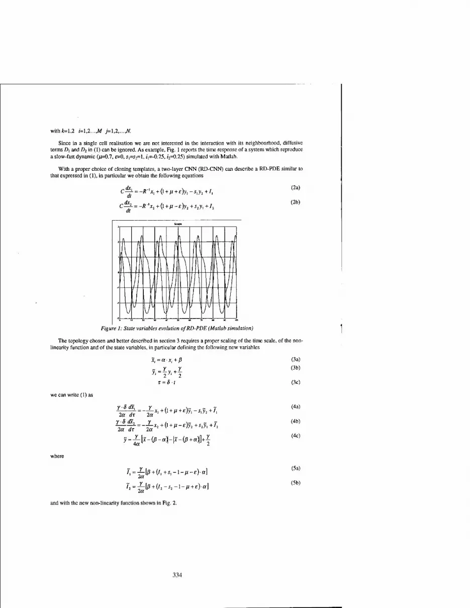
with/fc=l,2 i=\,l...M j=l,2,...N

Since in a single cell realisation we are not interested in the interaction with its neighbourhood, diffusive terms D\ and Di in (1) can be ignored. As example, Fig. 1 reports the time response of a system which reproduce a slow-fast dynamic (/*=0.7, e=0, Ji=i2=l, t'i=-0.25, «2=0.25) simulated with Matlab.

With a proper choice of cloning templates, a two-layer CNN (RD-CNN) can describe a RD-PDE similar to that expressed in (1), in particular we obtain the following equations

C-± = -R~'x, + (l + p + e)y, -sty2 + /, at

C—f = -«-' x2 +{l + n-e)y2 + s2yt +/2 at

(2a)

(2b)

Figure 1: State variables evolution of RD-PDE (Matlab simulation)

The topology chosen and better described in section 3 requires a proper scaling of the time scale, of the non- linearity function and of the state variables, in particular defining the following new variables

xt = a ■ x,. + ß

y, Y Y — y, + — 2 ' 2

t = S t

(3a) (3b)

(3c)

we can write (1) as

Y-8 dx. Y i. \~ 7

y-8 ax, Y ,, ■,_ _ r

y=-?-\x-(ß-a}-\x-(P+a]}+r

(4a)

(4b)

(4c)

where

/,=^-[i5 + (/1+i1-l-/i-E)-a]

/2=^[P + (/2-i2-l-// + E)-a]

(5a)

(5b)

and with the new non-linearity function shown in Fig. 2.

334

ß-oc ß+cc x

Figure 2: Non linearity function

3. VLSI Implementation

It is apparent that the RD-PDE in (4) can be realised by means of the single cell RD-CNN described in (2) with a proper choice of R, C and /;. Specifically, a block schematic of the single cell RD-CNN cell is shown in Fig. 3

h —k>

Figure 3: Block schema of the two-layer cell

It is worth noting that since state variables, %, are represented by a voltage and output variables, y,, are represented by a current, the non-linearity block is actually a bounded transconductor.

Blocks performing current multiplication between the output variables and constant values, such as ±s, or 1+JU±E, were implemented by means of 4-bit digitally programmable current mirrors. In the same way, also bias currents, /,, were realised by mirroring a constant current through two 8-bit programmable current mirrors. Cell programmability is required because of the different time evolutions that can be obtained by varying the cell parameters.

3.1 Non-linearity block and resistor implementation

The non-linearity block, which generates the cell outputs, is a bounded transconductor whose maximum current value, y, was set to 10 pA. As far as parameters a and ß are concerned, they were chosen in order to maintain the state variable, that is the voltage across the capacitor, in a proper bounded range between the ground and the power supply. A good choice was to set £»=150 mV and /5=1.6 V, respectively.

Referring to Fig. 4 the basic principle of the non-linearity block is to mirror the output current of the source coupled pair (M1-M2) by means of M3-M6 and to subtract the resulting current to /B2. This difference is mirrored again by M7-M8 and, after a further subtraction to Im, is driven to the output by means of M9-M10. By

335

setting IBI=20 UA and /s3=10 uA, the output current, Iy, will be bounded in the range 0-10 pA while the slope of the transcharacteristic will be set by a proper aspect ratio of M1-M2. In the actual implementation, all simple current mirrors were replaced by cascoded mirrors.

By comparing (4a-b) with (2a-b) it is apparent that the resistance value must be set to 2a/y and that the same value is used to define the transconductor slope (4c). This suggests that the cell resistors can be implemented by simply subtracting the transconductor current to the summing nodes for every layer of the cell in Fig. 3. This current is given directly by transistor M5 whose aspect ratio is equal to the aspect ratio of M6. It is worth noting that this approach will make the circuit less sensitive to parameter variations.

Figure 4: Schematic of the bounded transconductor

3.2 Time constant programmability

A time constant programmability is also required but, due to the very small capacitive value that can be integrated, the approach of using a programmable capacitive array is in contrast with the needing of very large time constants (in the order of a few seconds). Here two solutions to obtain a time constant programmability over a wide range are presented.

One solution controls the system evolution by means of a clock with a variable duty-cycle that let the system evolve during the positive phase and freeze the state value during the negative one. More specifically, referring to Fig. 5, during the positive clock phase the voltage capacitor is updated through the n-mos pass transistor, while the output of the buffer is floating. On the other hand, during the negative phase, the state across the capacitor is held and propagated through the buffer and the p-mos pass transistor. It is worth noting that, without transmitting the frozen signal, the rest of the cell would evolve without any control. In this way, the other variables of the cell are frozen too.

Figure 5: State variable capacitor and freezing circuitry

Charge injection, which modify the capacitor voltage when the n-mos transistor closes, and leakage currents, which discharge the capacitor during the negative phase, are the main drawbacks of this method. Both of them can be drastically reduced by using large capacitive values in the order of 10 pF.

The second solution proposed is shown in Fig. 6. The large time constant is obtained by connecting the state capacitor to the output of a unity-gain feedback OTA whose output impedance is increased by means of its current mirrors aspect ratios [8]. Indeed, referring to Fig. 6, all current mirrors (with the exception of M7-M8) reduce the mirrored current by a factor of M or N and it is easy to demonstrate that the output resistance is given by:

336

R™i — MN (6)

This resistance can be programmed by varying the factors M and N by means of programmable current mirrors or by modulating the bias current IB\ thus producing the required time constant programmability. By setting /B,=10 uA and the maximum value of both M and N to 225, the time constant can be programmed over more than 4 decades.

Even in this case the main limitation is given by the leakage current in the output branch. In particular the following relationship must hold for each value of M and N

/» 1-M-N

:»/;- (7)

fl^t» ^zS Figure 6: Schematic of the buffer with high output impedance

4. Validation results

The RD-CNN cell was implemented with a current-mode approach in a 0.35-u.m CMOS standard technology, supplied by STMicroelectronics.

The circuit was designed in the Cadence environment and simulated with ELDO. The cell parameters were

set to //=0.7, e=0, S]=l and s2=l- Bias currents, /; and T2, are set by applying (5) to the nominal bias current,

/i=-0.25 and /2=0.25, thus giving 7^=49 |iA and f2=51 |iA. This choice seems to be critical since the two

currents are very close each other and the cell itself is very sensitive to their variation. Actually, in a practical realisation, bias currents are given by an external trimmer, which is properly tuned until the desired behaviour is reached.

10 20 30 40 50

Figure 7: State variables evolution (with the delay block in Fig. 5)

Figure 8: State variables evolutions (with the delay block in Fig. 6)

337

The first simulation, depicted in Fig. 7, was performed by using the delay block in Fig. 5. The clock frequency was set to 100 Hz with a 100-ns positive phase. The time constant governing the cell evolution is increased by 100.000 times with respect to the natural time constant of the cell. The frequency of the slow-fast oscillation is close to 0.8 Hz.

The second simulation, shown in Fig. 8, was performed by using the delay block in Fig. 6 in which the ratios of the mirrors were set to their maximum value. In this case, the output frequency is close to 0.1 Hz.

5. Conclusions

A VLSI realisation of a double-layer single cell RD-CNN for motion control, which is based on the implementation of a few building blocks, was presented. The cell has a low sensitivity to tolerance variations and is able to reproduce the low frequency involved in motion control. More specifically, the tolerance problem was overcome by adopting the same transconductor core for both the non-linearity block and the resistor, while two different solutions were given for the realisation of very large time constants. The cell was designed with a current-mode approach in a 0.35-nm CMOS standard technology, supplied by STMicroelectronics. Both the two approaches were validated by simulating the cell with ELDO and by comparing the results with a Matlab simulation, thus showing a good agreement in the behaviour of slow-fast dynamics.

Acknowledgements

The authors wish to thank Prof. P. Arena and Ing. L. Occhipinti for their useful suggestions and encouragement.

References

[1] L. O. Chua, L. Yang: "Cellular Neural Networks: Theory and Applications", IEEE Trans, on Circuits and Systems, Vol. 35, N. 10, pp. 1257-1290, Oct. 1988. [2] L. O. Chua, L. Yang, K. R. Krieg: "Signal processing using Cellular Neural Networks", Journal of VLSI Signal Processing, N. 3, pp. 25-51, Jan. 1991. [3] P. Arena, S. Baglio, L. Fortuna, G. Manganaro: "Hyperchaos from Cellular Neural Networks", IEE Electronics Letters, Vol. 31, pp- 250-251, 1995. [4] L. O. Chua: "Special Issue on Nonlinear Waves, Patterns and Spatio-Temporl Chaos", IEEE Trans, on circuits and Systems - Part I, Vol. 42, N. 10, pp. 559-577, 1995. [51 T. Roska, L. O. Chua, D. Wolf, T. Kozek, R. Tetzlaff: "Simulating Nonlinear Waves and PDEs via CNN - Part I-ir, IEEE Trans, on Circuits and Systems, Vol. 42, N. 10, 1995 [6] P. Arena, M. Branciforte, L. Fortuna: "A CNN based experimental frame for patterns and autowaves", International Journal of Circuit Theory and Applications, John Wiley & Sons, Ltd., Vol. 26, pp. 635-650, 1998 [7] P. Arena, L. Fortuna, M. Branciforte: "Reaction-Diffusion CNN algorithms to generate and control artificial locomotion", IEEE Trans, on Circuits and Systems - Part I, Vol. 46, N. 2, pp. 253-260, Feb. 1999 [8] P. Kinget, M. Stayaert, J. Van der Spiegel: "Full analog CMOS integration of very large time constants for synaptic transfer in neural networks", Analog Integrated Circuits and Signal Processing, Kluwer Academic Publishers, Vol. 2, pp. 281-295, 1992 [9] A. Rodriguez-Vazquez, S. Espejo, R. Domlnguez-Castro, J. L. Huertas, E. Sänchez-Sinencio, "Current-mode techniques for the implementation of continuous-time and discrete-time cellular neural networks", IEEE Trans. on Circuits and Systems - Part II, vol. 40, pp. 132-146, Mar. 1993 [10] S. Espejo, A. Rodriguez-Vazquez, R. Domlnguez-Castro, J. L. Huertas, E. Sänchez-Sinencio, "Smart-pixel cellular neural networks in analog current-mode CMOS technology", IEEE Journal of Solid-State Circuits, Vol. 29, N. 8, Aug. 1994

338

2000 6™ IEEE International Workshop on Cellular Neural Networks and Their Applications Proceedings

Extended SC-CNN Implementation of the Hiridmarsh-Rose Neuron

Paolo Arena, Luigi Fortuna, Mattia Frasca

Dipartimento Elettrico, Elettronico e Sistemistico Universita degli Stud! di Catania

V.le A. Doria,«, 95125 Catanta - Italy E-mail: mfrasca@dees.unict.it

Abstract - In this paper an extended SC-CNN based design of the Hindmarsh-Rose neuron is presented. In particular, both the simplicity and low cost characteristic of the realisation are emphasised. Experimental series of this circuit are examined and either spiking-bursting behaviour or beating activity are observed for different values of a circuit parameter corresponding to a physical DC current in the biological model. Moreover, the implementation of the flexor-extensor Central Pattern Generator with the presented Hindmarsh-Rose neuron design is examined.

I. INTRODUCTION

Simple second or third order circuits, mimicking principal features of neurons, may constitute the cell for Central Pattern Generators in robotic applications [1]. In such studies different kinds of neurons have been used; in [2] numerical simulations of a Central Pattern Generator based on the Hindmarsh-Rose neuron [7] have been performed. From these simulation results the importance of having simple analog circuits showing neuron dynamics has arisen in view of their hardware realization. Second order CNN-based circuits, showing slow-fast dynamics similar to that generated in biological neuron firing activity, have been realised, in [6] an implementation of a neuron simple model of the Inferior Olive has been presented. This implementation was based on analog multipliers and so it was quite expensive. In this paper the possibility to have a low cost circuit able to mimic the Hindmars-Rose neuron is presented.

The Hindmarsh-Rose neuron conjugates the model simplicity with the complexity of the dynamics that the neuron exhibits. For different values of the external DC current input it is possible to observe either beating activity either spiking-bursting chaotic behaviour. The role of chaos in complex systems based on HR neurons (as the stomatogastric ganglion of the California spiny lobster) and the synchronous behaviour of two coupled HR neurons have been extensively studied [3][4]. The possibility of using a such type of neuron presents advantages connected to the wondering in different limit cycles concept. This is the reason for that a low-cost realization of the HR neuron may be important. For that purpose the SC-CNN paradigm is helpful. In [5], [8] and [10] it has been shown that SC-CNNs have a fundamental role in chaotic dynamics implementation, obviously such a type of realization requires only a few operational amplifiers and, so, it satisfies our low-cost need.

II. THE HR MODEL

The equations of the HR neuron are:

<& J., ^ — = y+<p(x)-z + I at

%=vW-y (i) dz — = -rz + r-S-(x-cx)

where:

(j>(x) = a-x2 -x3

y(x) = \-b-x1

0-7803-6344-2/00/$10.00 ©2000 IEEE 339

and the values of the parameters involved in (1) are: a = 3

A = 5

c, =-1.6

5 = 4

r = 0.0021 where x represents the membrane potential, y and z, a set of fast and slow ion channel respectively, I an

injected DC current. Typical values for I vary from 2-2.5 (quite regular spiking-bursting behaviour) to 3.281 (chaotic spiking-bursting behaviour). For higher values beating activity is observed.

In order to achieve feasibility of the implementation, equations (1) have to be rewritten as follows:

RC

RC

dX_ =

dx ~ \_dY_

5 dx 1 dZ

-Y + 1.5X'-6.25-X' 5 5 5

= 0.1- 3.125X" 5

(2)

AC——= -Z + 2(5Ar + 3.2) r dx

Equations (2) are obtained from equations (1) by introducing the positions:

X X

Y = [*]■ y = Z z

and

dx--

2/5 0

0 1/2

0 0

dt

RC

0

0

1

(4)

(3)

In the following sections it is shown that extended SC-CNNs may implement equations (3) and some experimental results are presented.

III. THE EXTENDED SC-CNN AND THE HR NEURON

Many generalisations of the classical CNN architecture introduced by Chua [9] have been proposed. In order to realise the Chua's circuit State Controlled CNNs (SC-CNNs) have been introduced [8]. Such structures were found able to represent a wide class of complex dynamics [10]. However, they can't map chaotic systems in which the non-linearities arc functions of two or more variables, and so the extended SC-CNN (ESC-CNN) have been introduced [5], In this section a further generalisation of this architecture is examined in order to realise the HR neuron model presented above.

The state equations of a cell C(i,j) of an ESC-CNN defined in a two-dimensional array of M by N cells are:

c~7r=-ir+ YUwyu+Btj-u-uu+c^-x^+it (5) "' Kx C(kJ)tNr(tJ)

with 1 <, i <. M and \<,j<,N and where the cell r-neighbourhood is defined by:

Nr (i, j) = {C(k, /)|max(|* - /|, \l-j\)<r) (6)

and the output yt. of the cell is a piece-wise linear ftinction that is dependent not only by the state Xtj, but

also by the state of the cells of his neighbourhood:

yi]=PWL( IX, W (7> C(k,l)EN,(i,j)

where the functions PWL stands for a piece-wise linear functions. In [5] the same PWL function is considered for each cell in order to realise a circuit implementation of the

Rössler system. In this paper this approach is generalized to consider different PWL functions, so the output is defined as:

C(l*»,(',/)

The HR neuron (3) may be realised by a such CNN constituted of only three cells. If it is assumed that these cells arc placed along a unique row, the sequent equations may be considered:

340

and

c(*)cJvr(o with / = 1..3. Equations (9) and (10) map the HR neuron (3) by considering:

(10)

V X V 7" V rpwx,«] *2 = Y ; «2 = 0 ; ^2 = P0X2()

*3. Z ."3. 0 .^S. 0 and choosing the templates as follows:

1 A,= [6.25 7.5 0l A2=—-[O -3.125 O] A3=—-[0 0 O]

Rx\ RX2 Rx3

B,=J-.[2/5 0 0} B2=-r^-[0 0 <>1 B3= —[o 0 o] Äxl Ä»2 Ä«3

1 1 c3=J_[io o o] C, =-^[l 4/5 -2/5l Cj=-— [0 4/5 0l Kx\ Kx2

01=J_.[! o 0l D2=~[\ 0 0} D3=~[0 0 0] K,, K-i Ar1

= 0; /, =0.1; /, = 6.4

PWLx(x)and PWL2(x) are piece-wise linear approximations of the function g(x) = x and

A(x) = -oc3 respectively. The implementation of these PWL functions needs only a few of OPAMPs and diodes. Fig. 1 show the trans-characteristic of the PWLs simulated in SPICE.

The time constants associated to each cell are different each other. These are chosen in order to respect the ratio between slow and fast dynamic of the variables. In Fig. 2 the overall circuit schematic is reported.

Fig. 1. (a) PWL approximation of x . (b) PWL approximation of-x

341

:■ :<••■

!** £ Di *y ^i" v-:-

_tsU -^/s*

-I I. I'" ■>"-* • ~ - r 1 f tk:i.

«5! !KK .]

■■*itr ."•••■Ä--4 ÄV .1

*Ji£E #-'!"

r|l f <)<•><: 5 ■J^'

r-n *. , ,,.,... r* '< .....: .,....,v,-....-. > :*<**:■:■:■:■:

Fig. 2. The HR circuit based on extended SC-CNN.

The HR circuit, discussed above, was realised with discrete components and the temporal evolution of the x,, the variable representing the membrane potential, was observed for different values of the parameter / . In

Fig. 3 some experimental results are reported. Moreover, also the beating behaviour has been observed for higher values of / than those ones reported in Fig. 3. These results match with the experimental series reported in [3]- [4].

x:.&c*$V? .I"^*^.?^*?;* S*?.*?.iKr."

GO

(b)

Fig. 3. (a) The spiking-bursting activity of the HR circuit for 1=1.7. (b) The spiking-bursting activity of the HR circuit for 1=2.44. The variable xl is plotted versus time.

342

rV. THE EXTENSOR-FLEXOR MODEL

One of the most simple Central Pattern Generators is the extensor-flexor model, depicted in Fig. 4a. It needs of only two neurons, mutually inhibited. A simple realisation of this system can be achieved by using two ESC- CNN HR cells and by modelling inhibitory synapses as in [3]:

-e-foiO + vJßM'-Tc)-*] where £ is the strength of the coupling, Vc the reverse potential, Tc is the synaptic delay, X is the threshold

and 0() the Heaviside function. It is assumed that the parameter values are those examined in [3]. In particular,

those ones referring to the membrane potential are scaled, the other ones are the same except for Tc that for sake

of simplicity is assumed to be zero. The parameters are reported below: e = 0.g;Fc=0.5;A' = 0.3

Our realisation of the inhibitory synapse is very simple and based on a MOSFET used as pass-transistor and a comparator. The whole system is reported in Fig. 4b, in which the blocks HR1 and HR2 indicate two HR neurons. They are the same that in Fig. 2 with a slight difference: the presence of a further resistor at node + of U6 A implies a different value for the resistor R21 (Ä21 = 45/Ki).

Fig. 4. (a) The Extensor-Flexor Central Pattern Generator, (b) The whole system for the extensor-flexor CPG.

It is assumed that / = 3.2 (chaotic behaviour) for both the neurons; moreover, they are characterised by different initial conditions. Fig. 5 shows the result of the SPICE simulation, a complete and in antiphase synchronisation is achieved.

In [4] it is shown that it is possible to achieve a complete and in antiphase synchronisation between the activity of the two neurons even if an artificial electrical synapse connects the two neurons. In this manner the whole system can be entirely realised by ESC-CNNs.

343

i «{t:xir :**»«*

Fig. 5. Synchronisation of the two mutually inhibited HR neurons. Variables xl of HR1 and HR2 are plotted versus time.

V. CONCLUSIONS

A lot of complex systems (for example other HR neuron based CPGs) can be generated starting by the design shown in this work. In this paper the ESC-CNN based HR neuron it was proposed which can constitute the fundamental unit for more complex biologically inspired neural networks. This kind of implementation avoids the use of analog multipliers by considering piece-wise linear approximation of the non-linearities in the HR model. Experimental results match theoretical observations, and, so, they confirm the suitability of this implementation. Moreover, the representation of the HR neuron dynamics by means of the ESC-CNN paradigm emphasises the key role of CNNs as a paradigm for the generation of complex spatio-temporal dynamics.

REFERENCES

[1] Arena P., L. Fortuna, M. Branciforte, 1999. "Realization of a Reaction-Diffusion CNN algorithm for locomotion control in an Hexapode Robot", Journal of VSLI Signal Proc. Systems, vol.23 n°21/3 Dec. 99.

[2] Arena P., L. Fortuna, D. Garofalo, 2000, "Simulation of Central Pattern Generators via Chaotic Neuron Populations", Proc. SYSID2000.

[3] Rabinovich M.I., H.D.I. Abarbanel, R. Huerta, R. Elson, A.I. Selverston, 1997, "Self-Regularization of Chaos in Neural Systems: Experimental and Theoretical Results", IEEE Trans. On circuits and systems Vol. 44, No 10, 1997.

[4] Elson R., A.I. Selverston, R. Huerta, N.F.Rulkov, MI. Rabinovich, H.D.I. Abarbanel, 1998, "Syncronous Behavior of Two Coupled Biological Neurons", Phisycal Review Letters 1998.

[5] Arena P., L. Fortuna, A. Rizzo, M. G. Xibilia, 2000, "Extending the CNN Paradigm to Approximate Chaotic Systems with Multivariable Nonlinearities", Proc. ISCAS2000.

[6] Arena P., L. Fortuna, M. Frasca, A. Giaquinta, 2000, "A New Circuit for Neuron Implementation", submitted to Nolta2000.

[7] Hindmarsh J.L., R. M. Rose, 1984, "A model for neuronal bursting using three coupled first order differential equations", Proc. R. Soc. Land. B, vol. 221, pp. 87-102, 1984.

[8] Arena P., S. Baglio, L. Fortuna, G. Manganaro, 1995, "Chua's circuit can be generated by CNN cells", IEEE Trans. Circuits & Syst. -Part I, vol. 42, ppl23-125, 1995.

[9] Chua L.O., L.Yang, 1998, "Cellular Neural Network: Theory", IEEE Trans. On Circuits and Systems, vol. . 35,pp.l257-1272, 1998.

[10] Manganaro G., P. Arena, L. Fortuna, "Cellular Neural Networks: Chaos, Complexity and VLSI processing", Springer-Verlag, 1999, ISBN: 3-540-65202-7.

344

2000 6™ IEEE International Workshop on Cellular Neural Networks and Their Applications Proceedings

A 2-D Conveyor Belt driven by a RD-CNN

L. Fortuna*, M. Branciforte**, L. Occhipinti**, S. Strazzuso, M.G. Xibilia***

*Dipartimento Elettrico, Elettronico e Sistemistico, Universitä di Catania V.le Andrea Doria 6,95125, Catania, Italy

e-mail: lfortuna@dees.unict.it **STMicroelectronics, R&D - Soft Computing Group

Stradale Primosole 50, 95121, Catania, Italy e-mail: marco.branciforte@st.com

***Dipartimento di Matematica, Universita' di Messina Salita Sperone 31,98166, Messina

e-mail: mxibilia@ingegneria.unime.it

ABSTRACT: in this paper a two-dimensional conveyor belt is controlled by neural processing approach; a particular CNN, named reaction-diffusion CNN, is used to generate waves propagation phenomena. They can propagate on the conveyor belt plane (an elastic membrane), moving an object between two points by a new kind of actuators: the Nitinol wires. A neural identification process of the membrane is illustrated to allow a suitable choice of the Nitinol dimensions. Moreover it is shown like both thermal and timing Nitinol behaviors are very similar to the slow-fast dynamics exhibited by a RD-CNN.

1. Introduction

Recently, the scientific community has been greatly involved in the study of complex phenomena, such as travelling wave fronts and autowaves. The possibility to deeply study such dynamics in order to draw its main rales opens the way to develop geometrically perfect structures characterized by intrinsic robustness against disturbances and noise, as it commonly happens in nature. The possibility to qualitatively reproduce such phenomena by using arrays of non-linear circuits as also allowed the simulation and artificial experimentation. Travelling wave trains have been observed in reaction-diffusion system with oscillatory kinetics. All the phenomena considered are reproduced by employing a simple two-layer CNN array with constant templates (RD- CNN) [1]. How it is shown in [2] an autowaves front can be quite interesting to reproduce locomotion in mechatronic devices. In particular in this paper we present a 2-D conveyor belt, built in our laboratories, to confirm the efficiency of the CNN approach. The mechanical structure is composed by an elastic membrane on which the autowaves can propagate, driven by a new kind of actuators, Shape Memories Alloys [3] (SMA's), in particular Nitinol wires. The paper is organized in two main parts: in the first one a briefly description of reaction-diffusion phenomena and their reproduction by CNN (RD-CNN) are discussed; in the second one the strategy adopted to drive the conveyor belt and the mechanical realization are described. Moreover the necessity of membrane identification and the use of a neural approach are justified. In order to drive correctly Nitinol wires, both its main thermal and timing characteristics are reported.

2. Reaction-Diffusion phenomena

Reaction-diffusion systems can be often found in living structures where transport processes take place, such as living neural tissues. These systems can be considered as a large number of identical coupled subsystems called cells. Each subsystem is defined through a set of non-linear differential equations [1], in particular:

-^- =-*vj +(l+M+eWi -Wvj +AU-,.; +Vu +^J-i +>Wi -4>w)+'i (la)

—T"=-%.; +(1+/'-fi)y*ü +*2>w+A(ya-.j +ya+u+JW-1 +>Wi -4>w.,)+'2 (lb> dt

where

fc=l,2 /=1,2...,M j=l,2 N (2b)

0-7803-6344-2/00/$10.00 ©2000 IEEE 345

With a suitable choice of the parameters <ji, e, s,, s2, i'(, i2, Dl and D2) [1], typical non-linear propagation phenomena, like autowaves and Turing patterns, can be described by the above equations.

2.1 Autowaves

Autowaves [4] represent a particular class of non-linear waves, which propagate without forcing functions in strongly non-linear active mediums. Their propagation takes place at the expense of the energy stored in the active medium. Autowaves possess some typical characteristics that are distinctly different from those of classical waves in conservative systems. Their shape remains constant during propagation whilst reflection and interference do not take place. Diffraction is common property between classical and auto waves. Next pictures shown an autowaves front.

Figure 1: An autowave front 2.2 RD-CNN

A CNN [5] is an array of simple non-linear systems called cells. With their analog and spatio-temporal distributed way to process signals, they are considered a powerful tool with which to generate real time solutions of non-linear partial differential equations (PDE's). With a proper choice of cloning templates, a two-layer CNN (called RD-CNN) can realise the system reported in (1) [1]. In this work, in order to obtain autowaves propagation, we utilise a RD-CNN simulator, developed in STMicroelectronics laboratories. Such software is also able to reproduce other complex phenomena like pattern formation (fig. 2).

(a) (b) Figure 2: Spiral wave (a); Pattern formation (b)

3. Two dimensional autowave driven conveyor belt

Autowaves can be very useful for motion control in automatic production chains [2]. In this novel kind of transportation system, the belt does not move in the direction of the destination of the object. Instead, propagation effect, due to the diffusion process, makes the effect of the belt to push the object toward its destination. This novel application of autowaves is quite interesting. In fact, autowaves proceed with unchanged amplitude and shape along the array and with no reflection and the direction of propagation can be driven cither

346

by suitable initial conditions or by modulating the path in real time via the CNN inputs. By suitably choosing the actuators, a two-dimensional conveyor belt driven by RD-CNN's can be shown to exhibit autowaves. This makes possible to realize arbitrary motions of objects from any given starting point to any other one by suitably modulating the CNN input mask that fixes the desired trajectories for the different objects. The mechanical structure of the conveyor belt is composed of two main parts: the first one is an elastic membrane on which an object can be moved; the second one is dedicated to stimulate the membrane with a new kind of actuators named Nitinol [3].

3.1 The elastic membrane

The RD-CNN approach causes a spatial discretization of the active medium on which autowaves take place, so it is necessary to create, on the elastic membrane, a grid of points (5x5) directly driven by the actuators (fig. 3). In this way each point of the grid can be moved up and down in order to obtain the movement of an object on the membrane.

Figure 3: The elastic membrane grid

3.2 Nitinol

There are two very common ways to create motion from electricity; motors and solenoids. However there is a very different and much newer way utilizing Shape Memory Alloys (SMA's). These special metals undergo changes in shape and hardness when heated or cooled, and do so with great force. In particular, Nitinol, a special SMA, pulls with a surprisingly large force and is capable of lifting thousands of times its own weight, whilst moving silently with a smooth, life-like quality. They can be heated with electricity and can be used to create a wide range of motions, operating quickly and with precise controllability. Nitinol has a uniform crystal structure that radically changes to a different structure at a distinct temperature. When the memory alloy is below this "transition temperature" it can be stretched and deformed without permanent damage, more so than most metals. After the alloy has been stretched, if it is heated (either electrically or by an external heat source) above its transition temperature, the alloy recovers or returns to the unstretched shape and completely undoes the previous deforming. When made into wires, SMA's can be stretched by as much as eight percent when below the transition temperature, and when heated, they will recover their original, shorter length, and contract with a usable amount of force in the process. In the next table it is shown how the recovering force is greater than the deformation force and that the force depends on the thickness of the wire.

Strength Nitinol 0.025 mm

Nitinol 0.050 mm

Nitinol 0.100 mm

Nitinol 0.150 mm

Nitinol 0.250 mm

Max recovery weight(g)

Recommended Recovery weight(g)

Recommended Deformation weight(g)

29

7

2

117

35

8

469

150

28

1056

330

62

2933

930

172

Table 1: Nitinol characteristics [31

347

3.3 Membrane identification

In order to choose a suitable Nitinol thickness and length, it is necessary to know the force that acts in each point of the grid fixed on the membrane. This means that it is necessary to characterize the membrane. Since it is a non-linear system and the boundary conditions are unknown, we adopted a soft computing approach to identify the elastic membrane. In particular we used a Neural Network with nine hidden neurons, in which the inputs were represented by 25 weights, one for each point of the grid, and the outputs were the change in position of the same points when the weights were applied to the grid. In every neurons the input signals are processed by a linear saturation activation function. Moreover we used a finite set of weights in the range [Og; 150g] with a step of 10g. In order to obtain the desired output error with a low number of learning patterns, we used a chaotic function (in particular the logistic function) which generates the same patterns. Since the output of the chaotic function can take values in the range [0; 1], we associated any values of the chaotic function to a weight in the range above defined. This enabled us to obtain a final output error equal to 3%. In fig. 4 there are depicted two samples of generic patterns not used for learning.

15 21

Real output: *; Goal: o

Figure 4: Error between real and model output

We used this neural model to obtain the minimum value of the force that the membrane applies in each point of the grid. This value is needed to choose the wire thickness of Nitinol with the right value of the deformation weight. Since the membrane must not apply a force that overcomes the recommended recovery weight, the neural model was used to help us find the maximum value of the excursion of each point based on the chosen fixed thickness (see tab. 1). Using the results from the neural model and the knowledge that Nitinol can be stretched by as much as 8%, a find length of the wire could be established.

3.4 The structure

Above considerations conduced to a Nitinol wire diameter equal to 0.1 mm and, consequently, a length of 18 cm. It was built a mechanical structure to connect Nitinol to the membrane. This structure allows controlling the mechanical tension of the wires (fig. 5).

Figure 5: The mechanical structure

348

This system is interfaced with the software simulator by an appropriate circuitry. This converts the digital output signal, sent in parallel port by the simulator, in an analog signal able to drive Nitinol wires. SMA characteristics strongly influence the wave shape of the control signal. In fact, Nitinol need a constant current to contract, so we must use a square wave. Moreover Nitinol possess different contraction and relaxation temperatures which determine the hysteresis shown in fig. 6. This graph shows the behavior of a Nitinol wire under a constant force. As the wire heats, its contraction follows the right-hand curve. When the temperature reaches Tcs the wire has started to shorten. When it reaches Tcf it is near full contraction. As the wire cools, it follows the left-hand curve, starting at the lower right and passing through T„ and Trf and the wire relaxes and lengthens.

^ > N

1 \ 1 1

li Hysteresis

i \i i

Figure 6: Nitinol histeresis

Practically both the changes occur over a small temperature. So an entire contraction-relaxation cycle shows a slow-fast dynamic where contraction and relaxation phases represent the fast regions and the phase between the two critical temperature (Tc, Tr) is the slow region. Since RD-CNN's exhibit slow-fast dynamic, output signals result a suitable choice to drive Nitinol wires. In the next picture it is shown the strategy adopted to generate control signal (b) by the slow-fast dynamic (a). Moreover it is shown how total programmability of the cellular neural network allows us to set the time evolution of each output in order to adapt itself to the Nitinol hysteresis time.

In fact when the output of the RD-CNN cell overcome the threshold level a constant current heats the Nitinol wire activating the fast contraction (Contraction time). In a second time the cell signal (a) goes under the threshold level, so Nitinol start to cool for a time necessary to reach the T„ temperature (Hysteresis time), we can set this time so that it corresponds to the slow region of the cell dynamic. At this point Nitinol fast relax itself in the Relaxation time described by the cell output signal (a). In this conditions the RD-CNN is able to generate the entire set of signal needed to drive the Nitinol array system in such a way to move an object in the belt by autowaves propagation.

Contraction lime (sec.) Hysteresis lime (tec) Relix.iion time (sec.)

Figure 7: RD-CNN state variable (a); Nitinol command signal (b)

349

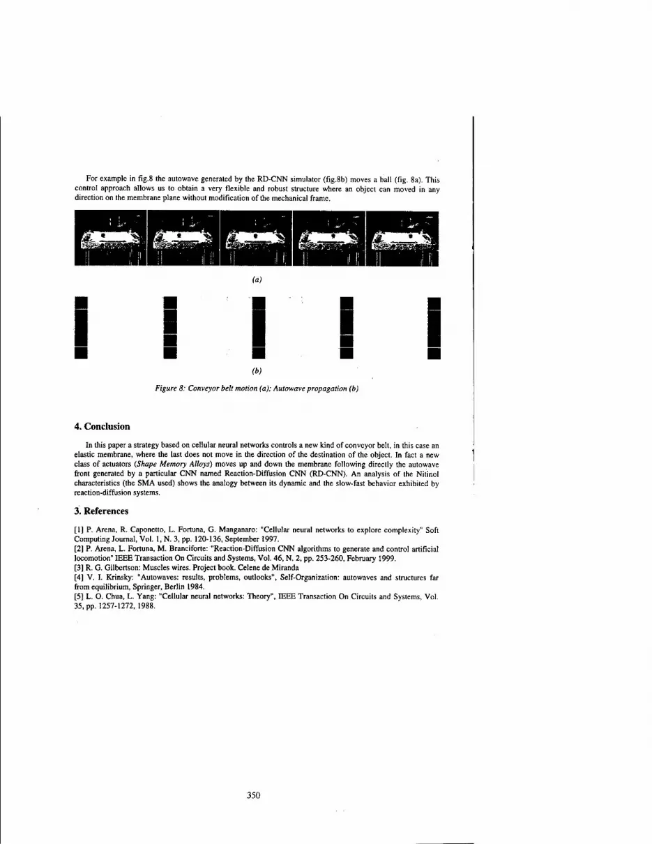
For example in fig.8 the autowave generated by the RD-CNN simulator (fig.8b) moves a ball (fig. 8a). This control approach allows us to obtain a very flexible and robust structure where an object can moved in any direction on the membrane plane without modification of the mechanical frame.

(a)

I I I I I (b)

Figure 8: Conveyor belt motion (a); Autowave propagation (b)

4. Conclusion

In this paper a strategy based on cellular neural networks controls a new kind of conveyor belt, in this case an elastic membrane, where the last does not move in the direction of the destination of the object. In fact a new class of actuators (Shape Memory Alloys) moves up and down the membrane following directly the autowave front generated by a particular CNN named Reaction-Diffusion CNN (RD-CNN). An analysis of the Nitinol characteristics (the SMA used) shows the analogy between its dynamic and the slow-fast behavior exhibited by reaction-diffusion systems.

3. References

[1] P. Arena, R. Caponetto, L. Fortuna, G. Manganaro: "Cellular neural networks to explore complexity" Soft Computing Journal, Vol. 1, N. 3, pp. 120-136, September 1997. [2] P. Arena, L. Fortuna, M. Branciforte: "Reaction-Diffusion CNN algorithms to generate and control artificial locomotion" IEEE Transaction On Circuits and Systems, Vol. 46, N. 2, pp. 253-260, February 1999. [3] R. G. Gilbertson: Muscles wires. Project book. Celene de Miranda [4] V. I. Krinsky: "Autowaves: results, problems, outlooks", Self-Organization: autowaves and structures far from equilibrium, Springer, Berlin 1984. [5] L. O. Chua, L. Yang: "Cellular neural networks: Theory", IEEE Transaction On Circuits and Systems, Vol. 35, pp. 1257-1272, 1988.

350

2000 6™ IEEE International Workshop on Cellular Neural Networks and Their Applications Proceedings

A Detailed Analysis of Different CNN Implementations for a Real-Time Image Processing System

K. Wiehler, M. Perezowsky, R.-R. Grigat

Technical University of Hamburg-Harburg Image Processing Systems

Harburger Schloßstraße 20, D 21079 Hamburg, Germany phone: +49 (0)40 428 78 -3536, -3125, fax: -2911 email: (k.wiehler,perezowsky, grigat}Otuhh.de

http://www.ti 1 .tu-harburg.de

ABSTRACT: A detailed analysis for different implementations of a real-time CNN signal processing systems is presented. The algorithm for signal reconstruction has been realized in hardware (analog VLSI, multi-FPGA system) and in software (TriMedia VLIW, Intel Pen- tium processor). All implementations are fully functional and embedded in a system envi- ronment. Due to the high computational complexity which is needed to solve the nonlinear CNN-equations and the requirements which are different for each application, an efficient implementation has to be tailor-made. In this publication we analyze different realized im- plementations regarding prototypical prerequisites.

1 Introduction

Due to the ongoing development of CNN-theory and applications [1,4] there is a great demand for a systematic analysis of different implementation alternatives. Especially due to the high computational complexity which is necessary to solve the nonlinear CNN equations in a real-time system1 we need special tailored solutions for each individual application.

The application requirements can be separated by the following points:

• Product costs: expenses for the system including system integration

• Design costs: design time, tool chain, level of automation

• Performance: accuracy, speed, power dissipation

• Flexibility: configuration, maintenance, update, future adaptation

• System integration: interfacing, environmental constraints

Each application emphasizes on different points: e. g. the costs of the final system are essential for a consumer market product, whereas used in a computer vision system as a preprocessing unit the accuracy of the results is most important.

In this publication we report on results we have achieved in implementing a simple nonlinear one dimensional regularization algorithm in different technologies: analog VLSI (0.8/im CMOS), multi FPGA-System (ASIC- prototype), TriMedia VLIW optimized C implementation and standard C code based on an Intel Pentium.

1.1 Outline of the Paper

In the following section the underlying nonlinear application is briefly described. The system requirements for an image processing system are specified. In the next section a short review of the Y-chart for System design (analog/digital VLSI, software) is given and the different implementations are introduced in more detail. For each technological alternative, comparable performance figures are calculated. The paper concludes with a summary of the results.

'With 'real-time' we denote a system which can process image sequences in standard video format.

0-7803-6344-2/00/$10.00 ©2000 IEEE 351

2 Theory and Application

In the present paper, we investigate realizations which compute the unique function u minimizing the following convex functional [7]:

J(v) = \J^{(v-g)2+\(\Vv\)}dx, (1)

for a given data g and the non-quadratic function

m ~ \ Xfe + (Aj - A?)c,(2( - c„), cp<t. (Z)

After applying a FEM-discretization on a one dimensional grid, the problem can be restated in CNN notation [8]:

vx,k = -Vz,k+ ^3 Ak,j[vxj,vx,k) + -(s/c-i +43t +ffjt+i) , (3)

with templates

j"e{fc—l,fc+l>

Ak,k-\ = -T(UI,*-1 -«x,*) + /("x,/c-l - "x.O (4) D

>W+i = -T(«j,w-»>,*)+/("i,Hi-»i,t)i (5) 6'

where

|x| < Cp /W-{ A^-KA^-A^sgnW |x| > 4 <6)

The described nonlinear regularization scheme can be used to reconstruct data in a noisy environment. Figure 1 and 2 give an example for ID and 2D data. The input data is corrupted by white and salt-n-pepper noise respec- tively. It can be seen from the results, that the noise is removed (blurred) while the salient signal parts (e. g. edges) are preserved. To save computational power in the 2D case the nonlinear filter has been applied in a row-by-row and column-by-column order.

Computational Complexity For each data point a nonlinear differential equation has to be solved. Therefore the order of the numerical complexity is O(N), with N the number of processed data points. To estimate the number of operations used to solve the equation a simple explicit Euler-method is used to solve (3). If we take Nop, for the number of operations used for the evaluation of one Euler iteration (3), and Ntt the number of iterations needed to get the result, the total number of operations per second is

OPS={Nop,NitN)f„

with /, the data rate in 1/sec. Taking a 25Hz frame rate standard video format with 576 x 720 = 414720 pixels (pixel rate 10.368MHz), Nu = 100 necessary iterations, and Nop, = 10 operations per equation evaluation, we need 10.4109 operations per second to cope with the data blast.

3 Implementation

3.1 System Design: analog VLSI, digital VLSI, Software

Implementation in terms of the Y-chart [3,2] means to start from a technology independent functional description and end up with a technology specific layout description.

It is obvious that for a realization in software the design flow ends with the implementation of the numeric algorithm. The rest of the design flow has been already done by the processor design. For a digital VLSI im- plementation using standard cells and state of the art CAD tools the domain is switched to the structural level by synthesizing a hardware description. From the synthesized RTL-level standard gate libraries and P&R-tools are used to proceed to a final layout description. In an FPGA-based design flow the placing and routing is performed under the FPGA macro cell constraints.

Unfortunately the level of automation in analog VLSI design is very low, and therefore the design flow has to take all levels with an essential support by the ingenuity of the design group. In figure 3 the Y-chart for an analog and digital System design is depicted. The 'stop'-signs denote where the 'engineer-driven' design ends and CAD tools give an essential support to the remaining design flow.

352

,tA AAA/1 r \J V

_M A^V~- r V r \j

1 -1 n y^i ■

\ u _J

Figure 1: ID signal example: noisy signal (left), processed signal (right), the salient edges are preserved while the noise is removed.

white noise / 'salt and pepper' noise processed image detected edges

Figure 2: 2D example for the nonlinear regularization algorithm used for the comparison of different implemen- tations (the images were 'computed' using the analog VLSI design). The algorithm removes the noise while the salient signal parts are preserved.

Function Functional desc.

Synthesis

Device \ Vrransisi

Component

anaVI^I(|^ou| BlocktMacro

Geometry

Algorithm

Concept

Cell

Roorplan

Partitioning

Figure 3: Y-chart for analog and digital system design. The analog specific parts are written in slanted letters while courier is used for the digital specific parts. The 'stop'-signs denote where the 'engineer-driven' design ends and CAD tools or a fixed architecture govern the remaining design flow.

353

3.2 Analog VLSI, 0.8/im CMOS

An aVLSI prototype in 0.8/im-CMOS has been designed and extensively tested [10, 9]. The design is based on a new architecture, which enables the analog circuitry to process signal vectors of infinite length (dynamic-CNN, dCNN). Due to this feature a video signal stream can be processed directly without an explicit serial to parallel conversion. The circuit works in strong inversion mode, consumes a power of approximately lmA@5Volt and requires about 30mm2 of silicon. The maximum sample frequency is 1MHz and independent of the rcgulariza-

Figure 4: Layout of the chip: 32 identical cells perform a nonlinear regularization; O.Sitm CMOS (Austria Mi- crosystems / AMS)

tion parameters. The power dissipation is more or less independent of the sample frequency due to the circular architecture of the implementation [10].

3.3 Digital VLSI, FPGA Lucent ORCA 2T40A

The algorithm has been also mapped on a multi-FPGA system ([5], figure 5). The CNN equation is solved by an explicit Euler procedure which has been implemented in VHDL. The synthesized result for 48 cells needs about

-^ . .__i...

Figure 5: A multi FPGA PCI-bus based system (left side of the PCB). Four FPGA modules are on each hoard. Four boards (16 FPGAs) can be used in parallel by a connective cross-bar switch. All devices arc programmed by using the PCI bus. A schematic of the core cell is shown on the right.

160kGates including all glue logic. The FPGA realization runs up to 14MHz iteration clock frequency. Taking JVjj = 48 • 2 = 9C this results in a 7MHz pixel clock frequency. If the VHDL is mapped directly to silicon, the clock frequency could be made noticeably larger.

3.4 Software: Pentium, TViMedia

Standard C-code and the Microsoft Visual C++ 5.0 C compiler has been used to implement the Euler scheme on an Intel-based PC. Using a Pentiumll with 300MHz, 2.52 million iterations have been evaluated per second. Taking Nit — 100 this results in a maximum pixel clock frequency of 25.2kHz.

ThcTriMcdiaTMlOOOis a 'programmable media processor'[6]. It is based on 'Very Long Instruction Word'- VLIW architecture which can perform up to 5 operations in one instruction. To support the TriMcdia compiler wc used loop unrolling and restricted pointers in the C code (surprisingly this 'hand-optimization' had no influence on the Pentium II performance). The TM1000 running with 100MHz performed 7.5 million iterations per second. Taking again Nu = 100 this results in a maximum pixel clock frequency of 75.8kHz.

354

4 Results

In table 1 the results of the different implementations are summarized. The throughput of the digital systems is calculated taking Nu = 100 iterations for the explicit Euler method.

analog VLSI FPGA (dig. VLSI) Pentium II TriMediaTMlOOO

Product costs

30mm2 in O.fyim CMOS; ss 60kGates (area equivalent)

4FPGAsORCA 2T40A, S3 140kGates

s» lMGates =3 300kGates

Design costs extremely high, full custom design

medium, VHDL, standard cell design

low, C program low-medium, optimized C-code

Performance: speed, accuracy, power dissipation

1MHz 8bit 5mW@5Volt

7MHz Sbit 3W@14MHz

25.2kHz 32bitFP 20W@300MHz

75.8kHz 32bitFP 6W@100MHz

Flexibility low, limited parameter variations

low-medium high high-medium

System integration

good in pure analog environment

good in digital environment

good(PC necessary)

very good: hardware interfaces for audio and video formats

Table 1: Summarized results for the different realizations. The best alternative in a row is marked with a box.

5 Conclusion In this contribution detailed results on different realizations (analog VLSI, digital VLSI, Intel Pentium II, Philips TriMedia) of a CNN algorithm used for image reconstruction are given. We separated the characteristics by: product costs, design costs, performance (speed, accuracy, power dissipation), flexibility and system integration. As expected there is no technology which behaves superior in all categories.

The digital VLSI design has the best performance in terms of data throughput. In an ASIC implementation it would perform real-time nonlinear image processing of a standard video format (576x720 @25Hz) where approxi- mately 10 Giga operations per second are necessary. Furthermore a digital implementation takes the full advantage of technology improvements.

If low-power and low-area are the main issues, the analog VLSI design performs best. It only uses 40% of the area and consumes less than 1 % of the power the digital counterpart needs.

Pure software implementations cannot cope with the amount of data in video processing systems. Although multi-media extensions combined with the versatileness of state-of-the-art RISC/DSP-cores greatly enhance the performance2, they cannot compete with application specific hardware.

2The TriMedia processor running with 100MHz is 3 time faster than the Pentium II running with 300MHz.

355

References

[1] Loen O. Chua. CNN: A Paradigm for Complexity, volume 31 of Nonlinear Science. World Scientific Pub- lishing, 1998. Series A.

[2] Dabuek D. Gajski and Donald E. Thomas. Silicon Compilation, chapter Introduction to Silicon Compilation. Addison-Wcsley, 1988. Y-Modell.

[3] B.J. Hosticka, W. Brockherde, R. Klinke, and R. Kokozinsli. Design Methodology for Analog Monolithic Circuits. IEEE Trans, on Circuits and Systems, 41(5):387-394,1994.

[4] Gabriele Manganaro, Paolo Arena, and Luigi Fortuna. Cellular Neural Networks: Chaos, Complexity and VLSI Processing. Number 1 in Advanced Microelectronics. Springer-Verlag, 1999.

[5] Michael Perezowsky. D-l: A runtime reconfigurable FPGA system. Technical University of Hamburg- Harburg, 1999. http://www.til.tu-harburg.de/~pere/Dl/Dl.pdf.

[6] Philips. TriMedia Homepage, http://www-us.semiconductors.philips.com/trimcdia.

[7] C. Schnorr. Unique Reconstruction of Piecewise-Smooth Images by Minimizing Strictly Convex Non- quadratic Functionals. Journal of Mathematical Imaging and Vision, 4:189-198, 1994.

[8] C. Schnorr, H. S. Stiehl, and R.-R. Grigat. On globally asymptotically stable continuous-time CNNs for adap- tive smoothing of multidimensional signals. In IEEE International Workshop on Cellular Neural Networks and their Applications, Sevilla, pages 351-356, June 1996.

[9] K. Wiehlcr, R.R. Grigat, J. Heers, C. Schnorr, and H.S. Stiehl. Real-time Adaptive Smoothing with a 1-D Non-linear Relaxation Network in Analogue VLSI Technology. In 20. DAGM-Symposium Mustererkennung, pages 341-348. Springer Verlag, 1998.

[10] K. Wiehler, R. Lembcke, R.-R. Grigat, J. Heers, C. Schnorr, and H.-S. Stiehl. Dynamic Circular Cellular Net- works for Adaptive Smoothing of Multi-Dimensional Signals. In IEEE International Workshop on Cellular Neural Networks and their Applications, London, pages 313-318, 1998.

356

2000 6 IEEE International Workshop on Cellular Neural Networks and Their Applications Proceedings

Linear Spatial Filter Design for Implementation on the CNN Universal Machine

Kenneth R. Crounse Chinling Wee Leon O. Chua

Dept. of Electrical Engineering, University of California, Berkeley, 94720 U.S.A. crounse®fred.eecs.berkeley.edu

Abstract: Linear spatial filtering is an important component of most image and video processing algorithms. Therefore, when designing CNN Universal Machine algorithms for image and video applications, it would be useful to be able to implement desired filtering operations on the hardware. Although it has been shown that any convolution mask can, in principle, be implemented by a series 0/3x3 template operations, such methods are time-consuming and error-prone. In this paper we investigate the use of simple CNN-UM algorithms involving only three filtering stages and using only 3x3 A- and B-templates to approximate desired filter transfer functions. The transfer functions for the structures are derived and a reduced parameterization is introduced. This form is conducive to optimization. Several examples are given wherein filters are designed to approximate a desired transfer function.

1 Introduction

Linear spatial filtering is a significant part of most of complex image processing algorithms. Since the CNN Univer- sal Machine (CNN-UM) is expected to be used in many image and video processing applications, implementation of arbitrary linear filtering operations is a important capability.

It has long been recognized that the B-template can be used for simple convolutions, but are limited to FIR filters of the same size as the template radius, typically of 3 x 3 support in real circuit implementations. By using the A-template, stable IIR filtering can be performed during a single CNN transient[l, 2], but only a limited class of filters can be implemented, again imposed by the limited degrees of freedom of the CNN templates.

We have been investigating the use of multiple CNN filtering operations to implement a wider range of filters by means of a CNN Universal Machine algorithm. In general, each stage is a CNN transient using A- and B-templates. Former methods which cascade B-template operations only can be considered as a special case[3, 4, 5]. Explicit transfer functions can be written in terms of the A- and B-templates for each possible sequence of series and/or parallel combination. Certain restrictions must be placed on the template elements to guarantee stability or a desired stability margin.

When approaching the design problem from an optimization point of view, it is important to eliminate redundant degrees of freedom as well as assign parameters that can be fixed by external filter design considerations. We show how arbitrary multiplicative constants can be removed even in the presence of constraints. Furthermore, a prototype filter design technique is used to account for pre-determined frequency-domain symmetry properties of the desired filter.

The basic design approach proposed is to consider a desired transfer function in the frequency domain. An optimization problem is then formulated depending on the number of desired stages and margin of stability (robustness). A nonlinear frequency-weighted least-squares optimization algorithm is utilized. The frequency- weighting scheme allows the designer some control of the relative importance of the various regions of the transfer characteristic. Heuristics for choosing the initial parameter vector for the optimization routine have been derived.

Several example designs have been performed. One- two- and three-stage CNN-UM algorithms were generated to approximate the ideal low-pass filter, a model human visual system (HVS) modulation transfer function, and a Gabor-type (Gaussian band-pass) filter. The results show that by using only 3x3 templates and only a few CNN filtering stages, excellent approximations can be found.

1.1 Single Transient Spatial Filtering

It has long been understood how the CNN can be used to perform linear filtering operations on input images. In particular, by use of the A-template, infinite impulse response (DR) filters can theoretically be implemented by

0-7803-6344-2/00/S10.00 ©2000 IEEE 357

a single transient[l, 2], If an infinite array is assumed, the two-dimensional Discrete Space Fourier Transform (DSFT) can be used to write a closed form solution to the dynamics, as long as the dynamics remain in the linear region (which for a stable filter can always be obtained by proper scaling). When using real CNN arrays with toroidal (wrap-around) or reflective (zero-flux) boundaries, the Discrete Fourier Transform and the Discrete Cosine Transform provide the proper representative basis.

We will assume an infinite CNN for ease of discussion. For simplicity assume that the A- and B- templates are origin symmetric, and Ä(wi, ui) represents the DSFT of the linearized A-template and B(UJI , u2) the DSFT of the B-template. Then, the linear dynamics of the CNN, which are exactly true within the CNN linear region, can be written:

h(u\,u2) ^ 0:

Xt(^,ui) = eK{u)uUJ2)tXo("uU2) + ,, ' , [eA(""-^)( - l] ß(Uu^)Ü(uu<^) Ü) A(ui,W2) L J

Ä(wi,w2) = 0: il(wi,W2) = Xo(u>\,iill) + <5(Wl,W2)Ü(Wl,U2) (2)

There are many possibilities for performing filtering operations with this system, e.g. by supplying data to the initial state and/or input, stopping the transient at chosen times, or allowing unstable linear operations. For our purposes we allow only steady state filtering in the stable linear region. It is clear for stability we must have Vui,W2,Ä(wi,W2) < 0. Then the CNN output in steady state will be:

X<x, (^i, u2) = y- -B(u),, U2)0(tJi, U2) (3) A(Wl,W2)

independent of the initial state. This relation between input and output can be interpreted as a transfer function:

til \ B(UI,U2) .. H(uuwi) = - -j- {- (4)

A(wi,w2)

The filter Ä(wi, ui) can be shown to have two important properties: 'zero-phase' and 'infinite impulse response'

(IIR). For our purposes, we define the stability margin of a stable CNN filter to simply be K = ™ jjfc1'^)). >-e-

the ratio of the maximum and minimum eigenvalues. The type of transfer function can be specified by choosing the elements of the A- and B- templates. Larger

template radii have increased degrees of freedom and can be used to design high-quality filters. Unfortunately, most CNN implementations will not allow larger than 3x3 templates, for which it is impossible to make good filters.

1.2 CNN Universal Machine Algorithms

The CNN Universal Machine is an architecture which allows the storage and combination of multiple CNN outputs. By using such an architecture it is possible to perform convolution by larger kernels by means of a decomposition into a sequence of small-template operations[3, 4]. In fact it is easy to show that any impulse response can be implemented, in principle, by using a series of only 3x3 B-template operations[5]. Unfortunately the method is, in general, not very practical since it involves a large number of operation where error may be accumulating. Many other relevant techniques, which approximate filters using small generating kernels, are also known [6J. However, they do not exploit the full capability of the CNN since they do not use the feedback A-template.

The goal of the following discussion is to approximate arbitrary transfer functions by combining a reasonable number of CNN transients using only a 3 x 3 A- and B- templates.

2 CNN Universal Machine algorithms for IIR filter implementation

In this section we will derive the effective transfer functions of simple CNN-UM algorithms for linear filtering. Algorithms using only up to three stages (CNN filtering transients) will be considered.

2.1 Formulation

For the simple series and parallel combinations being considered, there are seven distinct filter tree structures. For each, the overall transfer function can easily be expressed in terms of the transfer function of each CNN filtering stage. Such structures can easily be implemented on a CNN-UM with local storage and simple image addition. The seven filtering structures considered in our work are shown in Figure 1.

358

H,

H,

fp2.

G=H! _

H2 I— G = H1H2|sra!

IHK S^ I

,2—il3,zL„,,,, Figure 1: The seven filter structures considered in the paper along with the effective transfer function. Each block represents a single CNN filtering transient.

2.2 Reducing degrees of freedom

To understand the span of possible filters using such a structure, and for the purposes of synthesis, an efficient parameterization is required. Leaving the parameterization in terms of the template elements is not the most efficient since: there are redundant degrees of freedom, the conditions for template stability are obtuse, and it does not easily allow certain typical design characteristics to be easily fixed.

Here we address these issues by using the prototype filter method for template design[7,2], The templates are restricted to be linear combinations of a prototype filter c(»i, n2) and the unit impulse.

Ä(wi,u2) = aC(ui\, u;2) + 7 (5)

B(wi,ui) = ßÖ(u\,ui) + S (6)

The filter C(u)\,ui) therefore determines the contours of constant magnitude of the filter in the frequency domain. Using this strategy, the parameters which determine the contours of constant magnitude are pre-assigned by the choice of C, according to filter design problem being considered. A typical example would be to have circular symmetry, for which

0.25 0.50 0.25 c(ni,n2)= 0.50 [TO] 0.5 (7)

0.25 0.50 0.25

is a typical choice. In many of the filter structures being considered, some of redundant parameters are made transparent by using

the prototype filter form. For example, even in the single stage case, there is a multiplicative factor that can be distributed to either/both the numerator and denominator. Some care must be taken though to ensure that the A-template meets the stability margin requirement. To accomplish this, a necessarily positive value -7 can be factored out of the denominator of the transfer function giving:

ff(wi,w2) = a'C(uii,u>2) - 1 (8)

where 1 - Kmai < a' < 1 - -j^— is required to meet the stability margin. Eliminating this extra parameter results in three degrees of freedom per filtering stage. For serial and parallel

combinations of filters, another redundant parameter can be removed. This is most obvious in the serial case, but also applies to the parallel combination.

Finally, there is a redundancy introduced by the interchange of filters in symmetric structures. For example, swapping the position of two arbitrary filters in serial combination gives the same transfer function. Although this does not lead to the elimination of a parameter, it does mean that only half of parameter space need be searched.

359

2.3 Optimization Techniques

Given a desired filter transfer function characteristic, we would like to find a CNN filtering structure which can approximate it in three stages or less. The overall strategy will be to consider each of the seven structures separately and solve an optimization problem for each. Starting with the simplest structures, the one which first meets the error criteria will be chosen.

The general problem is a nonlinear constrained optimization. Many optimization schemes are possible, ranging from gradient decent based methods to genetic algorithms. The objective function is of the form:

\\W(UI,1J2) (6(uii,<*) - Hd(u>uu2))\\ (9)

where W(uii, W2) is a frequency-weighting function. This function can be used to give the designer the ability to designate certain aspects of the desired characteristic as critical. For example, in a low-pass filter design the transition band may be given a strong weighting to ensure a sharp cutoff. It should also be noted that various norms can be used in the objective function.

3 Experimental Results

To test the quality of the multi-stage filtering method as the number of stages is allowed to increase, several filters were designed. The constrained optimization routine from the Matlab toolkit was used to find a good local minimum to the error functions. The optimization was performed on a 64 x 64 sampling grid in the frequency domain. For all cases, a stability margin of Kmax = 10 was enforced, and a frequency-weighting function that normalizes the contribution of each annulus in the frequency domain was used. The sum of square errors was used as a norm.

The most difficult aspect of setting up the optimization problem was the choosing of the starting point in parameter space. A bad choice could lead to a significantly sub-optimal outcome, as the error surface has many local minima. We explored several techniques including random initialization, initializing the filters to all-pass, and initializing each filter to a linear estimate of its contribution to the overall transfer function.

Three filter types were investigated, all making use of using the nearly-circular symmetry of C(ui\, uii). The first was an ideal low-pass filter with cutoff frequency 0.46TT. The frequency weighting function was used to emphasize the transition region. The results, shown in Figure 2, can be directly compared to the single-stage CNN filter using 5x5 templates designed in [2].

A second useful filter in CNN applications is the human visual system (HVS) modulation transfer function (MTF). A result, shown in Figure 3, using three series stages provides a significant improvement on the single stage CNN filter used in [8],

Finally, a symmetric Gaussian band-pass type filter with desired peak frequency of 0.257T was designed. Unlike the previous examples, the general shape of the characteristic is very difficult, and was not achieved until three stages were used. The result is shown in Figure 4.

4 Conclusion

We have investigated the use of simple CNN-UM algorithms, involving three CNN filtering stages or less, to approximate desired linear spatial filtering operations. It was shown that the easily derived transfer functions can be cast into a form suitable for optimization methods. CNN-UM algorithms approximating some chosen sample filters were generated, and it was shown that the method produced good results.

Acknowledgments

This work was partially supported by the Office of Naval Research under Grant N0OO14-99-1-0959.

References

[ 1 ] B. E. Shi and L. O. Chua, "Resistive grid image filtering: Input/output analysis via the CNN framework," IEEE Transactions on Circuits and Systems - /, vol. 39, pp. 531-548, July 1992.

[2] K. R. Crounse and L. O. Chua, "Methods for image processing and pattern formation in Cellular Neural Networks: A Tutorial," IEEE Transactions on Circuits and Systems - /, vol. 42, pp. 583-601, Oct. 1995.

360

[3] S. Schwarz, A. Rotter, and W. Mathis, "Composition and decomposition oflocal operators for Cellular Neural Networks," in KleinheubacherBerichte, Band 37, pp. 253-262, Oct. 1993.

[4] K. Slot, "Large-neighborhood template implementation in Discrete-time CNN Universal Machine with a nearest-neighbor connection pattern," in Proceedings of the Third IEEE International Workshop on Cellular Neural Networks andTheir Applications,^. 213-218, Dec. 1994.

[5] K. R. Crounse and L. O. Chua, "Arbitrary spatial convolution via the CNN Universal Machine with 3 x 3 templates: Methods and issues," Memorandum UCB/ERL M96/5, University of California at Berkeley Electronics Research Laboratory, Jan. 1996.

[6] J. F. Abramatic and O. D. Faugeras, "Design of two dimensional fir filters from small generating kernels," in Proceedings of the IEEE Conference on Pattern Recognition and Image Processing, pp. 116-118, May 1978.

[7] J. S. Lim, Two-Dimensional Signal and Image Processing. Englewood Cliffs, NJ: P T R Prentice Hall, 1990.

[8] K. R. Crounse, T. Roska, and L. O. Chua, "Some methods for practical halftoning on the cnn universal machine," in Fifth IEEE International Workshop on Cellular Neural Networks and Their Applications, Proceedings, pp. 337-342, Apr. 1998.

j lr-J/4 l

1 I '■ ': \ ' ideal

/: i ' :\ designed

:xJJ\\ ! fe -0.5 -0.375 -0.25 -0.125 0 0.125 0.25 0.375 0.5

spatial frequency (cyclesj^ixel)

Figure 2: An ideal low pass filter and the designed filter, shown along the u\ axis. This filter uses an S3 filter structure.

361

if \\ w*8'

1 / ; \ j V

-0.5 -0.375 -0 25 -0125 0 0.125 0.25 0 375 OS spatial frequency (cydes^bcal)

Figure 3: An ideal HVS model filter and the designed filter, shown along the U-M axis. This filter uses an S3 filter structure.

Figure 4: An ideal Gaussian band-pass filter centered at 8 pixels/cycle and the designed filter, shown along the t axis. This filter uses an P3 filter structure.

362

2000 6™ IEEE Internationa] Workshop on Cellular Neural Networks and Their Applications Proceedings

Design and Training of Multilayer Discrete Time Cellular Neural Networks

for Antipersonnel Mine Detection Using Genetic Algorithms

P. Lopez', M. Balsi+, D.h. Vilarino' andD. Cabello* •Department of Electronics and Computer Science

E-15706, Santiago de Compostela, Spain Tel: +34 981 563100 Ext: 13559; Fax: +34 981 599412

E-mail: paula@dec.usc.es, dlv@dec.usc.es, diego@dec.usc.es +Inter-University Center for Research on Cognitive Processing in Natural

and Artificial Systems and Department of Electronic Engineering "La Sapienza" University, Via Eudossiana 18,1-00184, Rome, Italy.

Tel: +39 06 44585485; Fax: +39 06 474 2647 http://tce.ing.uniromal .it/balsi.html

ABSTRACT: In this work we present a novel strategy for the simultaneous design and training of multilayer Discrete-Time Cellular Neural Networks. This methodology is applied to the detection of surface-laid antipersonnel mines in infrared imaging. The procedure is based on the application of Genetic Algorithms for both network design and learning tasks.

1 Introduction

The United Nations estimate that probably more than 110 million land mines have been laid world-wide in more than 60 countries causing that thousands of people are killed or injured every year [1]. So, the development of a quick and reliable methodology for the determination and identification of antipersonnel mines (APM) is of crucial interest.

Different techniques exist that approach this problem. One of the most promising ones is the use of infrared imaging which yields information about temperature differences due to the different thermodynamic properties of the buried mine and the surrounding background. Infrared radiometers are sensors that measure and record the thermal radiation of different objects that is both a function of its temperature and of the emittance of its radiating surface. The thermal contrast of an object with respect to its environment is thus a function of these two parameters, both of the object and of its background, and varies in proportion to the duration of heating. In [2] an approach to produce an image with enhanced contrast between the objects due to the dynamic behaviour difference is presented on the basis of which a discrimination between different object types is derived. This approach was mainly based on principal component extraction and the Kittler and Young Transformation. In this set of experiments, the 24 hour cycle of an APM placed just below the surface was followed and images were taken every'30 minutes. Although the results obtained with this technique are very promising, they are still not able to obtain totally reliable results and have the disadvantage of using a very large sequence of images, what is very time consuming. Morover, it constrains the infrared camera to be located in the same position for a long time, which results in a reduced time-efficiency.

On the other hand, Cellular Neural Networks (CNN) are characterized by the parallel computing of simple processing elements, locally interconnected [3]. This fact, along with its possible implementation as an integrated circuit, makes them a very suitable tool for those image applications requiring high processing speeds, in which the processing is restricted to the neighbourhood of each pixel. Morover, its discrete time extension (DTCNN) is characterized by a synchronous processing that allows a robust control over the propagation velocity, making the extension to multilayer structures easier [4],[5]. These characteristics of high speed image processing and easy multilayer extension (that allows tackling of complex problems) make them an interesting alternative for the problem of APM detection.

To approach a given task by means of a CNN architecture, the weights of the connections among cells must be determined. This can be done either heuristically or by means of a learning algorithm that leads to good solutions on single layer CNN, but often fail when multiple CNN operations are required. In addition, for multilayer structures its highly complex dynamical behaviour makes most of the learning algorithms applied to single layer structures unsuitable and the training is usually done layer by layer, which requires an explicit knowledge of the exact behaviour of each of them.

0-7803-6344-2/00/$10.00 ©2000 IEEE 363

In this work we propose an algorithm for the simultaneous design and training of DTCNN-type architectures based on the use of Genetic Algorithms (GA). The proposed algorithm is able to find not only the network pa- rameters but also the network topology that best fits the problem. This is a general purpose algorithm, and no assumption is made about the specific domain of application. However, to demostrate its capabilities, it is applied to the problem of APM detection.

In Section 2, a brief description of the proposed algorithm is done. Section 3 shows the first results obtained with the basic algorithm configuration and in Section 4 some algorithm improvements are presented. Conclusions of the work are given in Section 5.

2 Algorithm Description Finding the set of parameters that best fits a problem is one of the core problems in the field of neural networks. Deterministic methods offer good results when the problem has a limited complexity, but for complex tasks they become usually slow and can be easily misled by local minima. Moreover, they require an exact knowlege about the function to be optimized that is not always available. In such a situation, stochastic learning algorithms and, particulary, Genetic Algorithms become and interesting alternative [6]. GAs have been successfully applied to the problem of CNN training. In those works only the weights of a fixed-size structure ([7], [8],[9]) or even the number of layers for a given connection scheme ([10]) were optimized. Here we present a general purpose algorithm that also finds the network topology that best fits the problem under consideration. This algorithm is independent on the particular domain of application but here the problem of APM detection on infrared imaging will be considered as an example of application.

As it was explained in the previous section, infrared images of APM-infested lands show the information about temperature differences due to the different fhermodynamic properties of the buried mine and the sur- rounding background. After applying an external thermal stimulus, either natural (sun radiation) or artificial, the heating/cooling process will follow the general equation of heat conduction that states that the variation of the temperature of an object with time is proportional to its thermal diffusivity. Since the heating/cooling process of the APM is different from those of other objects present in the scene, using a sequence of images at different time intervals should allow to separate the mine from the environment on the basis of their different thermodynamic behaviour. The images used were obtained from a database of the ETRO-KIS group of the Department of Elec- tronics of the Free University of Brussels. In this database, images taken every fifteen minutes are stored, one of which is shown in Fig.l. As can be seen, these are very complex images with the presence of lumps of land, stones and other buried objects, which make that the exact location of the mine can not be directly extracted.

Figure 1: Infrared image of a mined land.

To show evidence of the different thermodynamic behaviour of the mine and its background, we made use of the system shown in Fig.2. A sequence of four images during the heating process (represented as U1,...,U4 in the figure), from 10:45 to 11:30 a.m., was taken as the external input of the reconfigurable network structure. The original images are of size 768x375 but, for velocity reasons, only small pieces of size 155x80 were used during the training phase. This sub-images were taken in such a way that not only part of the mine but also of the background were present. The corresponding desired output (shown as ya in Fig. 2) is a binary image where black pixels correspond with the location of the mine in the scene and is obtained "by hand" because the exact coordinates of the mine are unknown. This image will be used by the GA to measure the validity of the solutions, which code candidate network configurations together with its template coefficients. This is done by comparing the resulting network output obtained with a specific configuration with the ideal output. A fitness

364

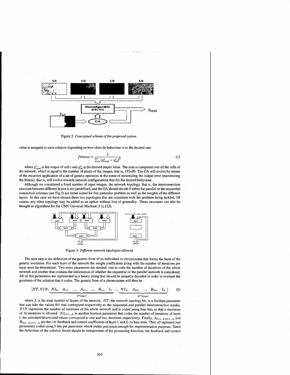
real

Figure 2: Conceptual scheme of the proposed system.

value is assigned to each solution depending on how close its behaviour is to the desired one:

fitness = 1

Ec (s£ ■vur (1)

where ycreal is the output of cell c and yc

id is the desired output value. The sum is computed over all the cells of the network, which is equal to the number of pixels of the images, that is, 155x80. The GA will evolve by means of the recursive application of a set of genetic operators in the sense of minimizing the output error (maximizing the fitness), that is, will evolve towards network configurations that fits the desired behaviour.

Although we considered a fixed number of input images, the network topology, that is, the interconnection structure between different layers is not predefined, and the GA should decide if either the parallel or the sequential connection schemes (see Fig.3) are better suited for this particular problem as well as the weights of the different layers. In this case we have chosen these two topologies that are consistent with the problem being tackled. Of course, any other topology may be added as an option without loss of generality. These structures can also be thought as algorithms for the CNN Universal Machine [11], [12].

til JtilSil JLU Ml j 1 M2 [| M3 | | M*

I Nl Ui I k"L_j*z_jN

r^T

~w Figure 3: Different network topologies allowed.

The next step is the definition of the generic form of an individual or chromosome that forms the basis of the genetic evolution. For each layer of the network the weight coefficients along with the number of iterations per layer must be determined. Two extra parameters are needed: one to code the number of iterations of the whole network and another that contains the information of whether the sequential or the parallel network is considered. All of this parameters are represented in a binary string that should be properly decoded in order to evaluate the goodness of the solution that it codes. The generic form of a chromosome will then be

[NT,NIN, NIU Ai NIL, AL1, BLK, It (2)

l'Hayer Lthlayer

where L is the total number of layers of the network. ATT, the network topology bit, is a boolean parameter that can take the values 0/1 that correspond respectively to the sequential and parallel interconnection modes. NIN represents the number of iterations of the whole network and is coded using four bits so that a maximun of 16 iterations is allowed. JV/I=I...L is another boolean parameter that codes the number of iterations of layer /, the activated/deactivated values correspond to one and two iterations respectively. Finally, Ai=i..i i=i...„ and Bi=i..L,i=i...n are the i-th feedback and control coefficients of layer /, and /; its bias term. They all represent real parameters coded using 5 bits per parameter which yields precission enough for implementation purposes. Since the behaviour of the solution found should be independent of the processing direction, the feedback and control

365

templates are supposed to be symmetric, and thus only three coefficients per matrix must be optimized, given n = 3. This results in an important reduction in the number of template coefficients that must be optimized, from 19 to 7 for each layer. The total chromosome lenght will then be of 257 bits.

3 First Results

We used a classic non overlapping GA with elitism, two point crossover, mutation and crossover rates of 0.10 and 0.70 respectively and a population size of 500. With this specifications, a solution with a 1.7% relative error is reached after 2400 iterations of the algorithm. This solution corresponds to a parallel connection scheme (NT = 1) with four iterations of the whole structure (NIN = 0100 =' 4'). Each of the seven layers of the network perform a single iteration (NIi = 1V7 = 1...L). The solution found properly decoded is shown in equation 3 where the parameters are written following the notation of the string introduced in equation 2.

W = [1,4,1, -0.48,1.13, -4.68,0.80, -3.39, -5.0, -2.74,1, -2.42, -3.71, -0.48,4.0,1.77,-1.13,0.81,

1,0.48,3.39,-1.13,5.0, -3.10, -0.48,4.35,1,0.48,2.74, -4.68, -3.39,5.0, -3.39,2.42

1, -2.10, -3.10, -5.0,0.48,2.74,-1.77,4.35,1,3.71, -4.03, -4.03,4.68,2.42, -0.48,2.10

1, -0.48,2.10,3.72,0.16, -2.42, -2.74,1.13] (3)

Applying this solution to the whole images of size 768x375, at the same time intervals considered during the training, we obtain the output shown in Fig.4. As can be seen, the network is able to generalize the result to the complete scenario. The output of the network is a black and white image where the exact position of the mine is precisely defined. Thus, not only the presence of a mine can be detected, but also its size and shape, which could help during the mine clearance process.

Input Sequence

10:45 11:00 11:15 =>

Optimized Network =>

I

Figure 4: Network output when the input sequence 10:45-11.00-11:15:11:30 is used.

In order to evaluate the robustness of the network, we considered two situations. First we applied as input two sequences of images shifted in time obtainig the results shown in Fig. 5(a) and (b) respectively. As can be observed in the output images, although the contour of the mine is not so well defined as in the previous case, it is still perfectly distinguishable from the background. This result is very important because the need of an absolute precision in the time of acquisition of the images will make its application very restrictive.

¥

(a) (b)

Figure 5: Outputs with time shifted input sequences: (a)10:45-l 1:15-11:45-12:15; (b)10:30-l 1:00-11:15-11:30.

The second situation we have considered is the robustness of the network when the input images are corrupted by gaussian noise. Two different cases have been considered with mean zero and deviation values of 0.01 and 0.1. The outputs obtained are shown in Fig. 6. As can be seen, the system is immune to the presence of small quantities of noise (Fig. 6(a)), but when this is important, a significative distortion in the output of the network is observed (Fig. 6(b)). Nevertheless, the location of the mine is still perfectly distinguishable, and the impurities that appear can be easily removed with some type of filtering since most of them correspond to spurious black pixels.

366

f" essrssf

'.■''■. .-.,. **:r '■■■ ■' *•.%

(a) (b)

Figure 6: Outputs with the input sequence corrupted by gaussian noise of x = Oand: (a) a = 0.01; (b)a = 0.1

4 Algorithm Improvements

4.1 Random selection of the training patternes

The selection of the training patterns is of crucial importance in order to guarantee the generalization capabilities of the network. In the basic algorithm it was done by hand, selecting a piece of the original image that contains information about the mine and the background. In order to improve the generalization capabilities of the solution found we have modified the basic configuration of the algorithm, allowing it to use different pieces of the image, randomly selected, in each iteration of the GA. So, in this case, the whole images will be applied as the inputs of the network during the training phase although in each iteration only small pieces, randomly selected, will be used for evaluation purposes. Since the part of the image corresponding to the mine position is small compared with the global image, we have defined two different areas on the image: one corresponding to the mine and the other to its surrounding environment. In each iteration, a piece of each area will be randomly selected in such a way that their global size is equal to the size of the images used previously, that is, 155x80..

Doing this, after only 73 iterations of the algorithm a solution is found that totally minimizes the error on the training set. As in the previous case, this solution also corresponds to the parallel connection scheme shown in Fig. 3 but with different template values. The output of the system in this case is shown in Fig. 7(a).

4.2 Automatic selection of the input images

In order to extract the information contained in the thermal contrast between the different objects present in the scene, we have considered a fixed sequence of images as the input of the network. Since all the images are close in time, we expect a redundancy of information content. In order to avoid the processing of useless information which can be very time consuming, we gave the algorithm the possibility of selecting only those inputs of the training pattern that are sufficient to match the desired output.

Doing this, and repeating the training process with the same training set, we found a solution that makes use of only two of the input images (namely those of the 10:45 and 11:15) without significatively increasing the error (2.6% in this case). The output obtained in this case is shown in Fig. 7(b). This strategy, allows us to initialize the training set with a large sequence of images (in order to accurately reflect the thermodynamical behaviour) without being afraid of needing a too large network size since the GA will be able to discard those redundant or dispensable entries.

r7? ••••?' (a) (b)

Figure 7: (a)Network output with random selection of training patterns. (b)Network output with automatic selec- tion of input images.

367

5 Conclusions

We have developed a general purpose algorithm for the simultaneous design and training of complex DTCNN architectures, here applied to the problem of APM detection in infrared images. This technique has the advan- tage of being implementable as a dedicated integrated circuit which meets the requirements of small size, low consumption and high processing speeds. Morover, even without dedicated electronic implementation, all the processes can be simulated on a common PC in a few seconds due to the discrete time nature of the network, or even thought as algorithms for the CNN-UM. Obviously, the training process should be repeated for any new physical environment (i.e., presence of vegetation, different soil characteristics...) and/or different athmosferic conditions, which means one or two hours of computation. This is a reasonable amount of time compared to the acquisition time as long as for the training only small pieces of images are needed while the resulting network can be applied to the whole mined land of arbitrary dimension.

Acknowledgement

Thermographic images used in this work were kindly provided by the ETRO-IRIS group of the Department of Electronics of the Free University of Brussels (http://etro.vub.ac.be/minedet/). Assistance of Prof. H. Sahli and Mr. L. van Kempen is gratefully acknowledged.

References [I] Federal Ministry for Education, Science, Research and Technology of the Federal Republic of Germany.

International Workshop and Study on the State of Knowledge for the Localisation and Identification of Anti- Personal Mines, 1994. ISP 9501.

[2] M. Schachne, L. van Kempen, D. Milojevic, H. Sahli, Ph. van Ham, M. Acheroy, J. Cornells: "Mine Detection by Means of Dynamic Thermography: Simulation and Experiments". IEE Second International Conference of Abandoned Landmines (MD'98), pp 124-128, October 1998.

[3] L. O. Chua and L. Yang, "Cellular Neural Networks: Theory". IEEE Transactions on Circuits and Systems, vol 35, nlO.pp 1257-1272, October 1988

[4] H. Harrer and J. A. Nossek, "Discrete Time Cellular Neural Network", International Journal of Circuit Theory and Applications, vol 20, pp. 453-467,1992

[5] H. Harrer, "Multiple Layer Discrete Time Cellular Neural Network Using Time Variant Templates", IEEE Transactions on Circuits and Systems-II: Analog and Digital Signal Processing, vol 40, n.3,pp 191-199, March 1993.

[6] D. E. Goldberg, "Genetic Algorithms in Search, Optimization and Machine Learning" Addison-Wesley Pub- lishing Company, January 1989.

[7] T. Kozek, T. Roska and L.O. Chua, "Genetic Algorithm for CNN Template Learning". IEEE Transactions on Circuits and Systems-I: Fundamental Theory and Applications, vol. 40, n.6, pp. 392-402, June 1993.

[8] T. Sziränyi, M. Csapodi, "Texture Classification and Segmentation by Cellular Neural Networks using Genetic Learning". Computer Vision and Image Understanding, (CVIU), vol. 71, n. 3, pp. 255-270, 1998.

[9] P. Lopez, D.L. Vilarino and D. Cabello, "Genetic Algorithm Based Trainig for Multilayer Discrete-Time Cellular Neural Networks ". International Work-Conference on Artificial Neural Networks, Lecture Notes in Computer science, vol 1607, pp. 467-476, Springer-Verlag, Berlin, 1999.

[10] P. Lopez, D.L. Vilarino and D. Cabello, "Design of Multilayer Discrete Time Cellular Neural Networks for Image Processing Tasks based on Genetic Algorithms". Accepted for publication in ISCAS'2000.

[II] T. Roska and L.O. Chua, "The CNN Universal Machine: An analogic array computer". IEEE Transactions on Circuits and Systems, vol 40, pp. 163-173,1993

[12] T. Roska, L. Kek, L. Nemes, A. Zarändy, M. Brendel, "CSL-CNN Software Library, DNS-CADET-15", Analogical and Neural Computing Laboratory, Computer and Automation Institute, Hungarian Academy of Sciences.

368

2000 6™ IEEE International Workshop on Cellular Neural Networks and Their Applications Proceedings

A New Synthesis Procedure of Cellular Optimal Linear Associative Memories for Robot Vision Systems

MicheleBRUCOLf, Donato CAFAGNA'', Leonarda CARNIMEO'

*Dipartimento di Elettrotecnica ed Elettronica - Politecnico di Bari viaOrabona, 4 -70125 Bari (Italy) E-mail: carnimeo@deemail.poliba.it

ABSTRACT: A design procedure of discrete-time cellular neural networks (DTCNNs) to be used as associative memories for robot vision is presented. The choice of cellular neural networks is motivated by their architecture, suitable for storing images, and their locally connected structure, which is effective for the hardware implementation of the designed memories. In particular, taking into account the constraints dictated by the discrete-time cellular neural networks structure, in this paper a design procedure of DTCNNs, which also enables memories to recognize correctly the event of superimposition of tools, is developed. To this purpose, a cellular associative memory which behaves as an optimal linear associative memory (OLAM) is synthesized. The performances of the designed network are investigated and its behaviour as an optimal linear associative memory is confirmed by means of an example of recognition of superimposed tools handled by a robot in an assembly line.

1. Introduction

In the field of robotics real time image processing is fundamental, as it usually provides the information necessary for the execution of a robot task. Since a robot acts on the basis of image analysis, the results of a recognition process required from a robot must possess a high degree of safety. As a consequence, constraints in object matching have to be established by means, of suitable techniques to assure the extraction of information specifically required for the robot to carry out its job. In this work the problem of designing a network which has to recognize industrial tools for a robot vision system has been dealt with [1,2]. More in detail, a robot has been considered which involves a camera positioned above a conveyor belt to capture images of some industrial tools moving on the belt, an image processing neural system and a robot arm, which must catch the industrial tools from the belt for utilizing them. The image processing neural system is based on the behaviour of an associative memory which realizes the necessary real time object matching of tools by comparing detected images and reference memorized ones. However, unusual situations can occur if tools casually superimpose one another on the conveyor belt. A particular attention must be reserved to this case, which has to be classified as an emergency situation by the robot. On the basis of these considerations, in this paper a design procedure of discrete-time cellular neural networks (DTCNNs) [3-6], which also enables memories to recognize correctly the event of superimposition of tools, is developed. To this purpose, a cellular associative memory which behaves as an optimal linear associative memory (OLAM) is proposed [7]. In particular, a theoretical explanation of the behaviour of optimal linear associative memories is firstly provided. Then, by considering binary images as bidimensional patterns to be stored into the cellular network, a synthesis procedure based on pseudoinversion techniques is presented.

Finally, the performances of the synthesized cellular OLAM are evaluated by carrying out a simulation example of recognition of industrial tools handled by a robot in an assembly line, also in the case of superimposed tools. Considerations about the error correction capability are also reported.

2. Optimal Linear Associative Memories

In this section m pairs of binary vectors (x\ /) are considered, where x' has lenght n and / has lenght n+1. These vectors have to be associated by means of a memory in such a way that:

y'=Mx' i'=l,..., m (1)

0-7803-6344-2/00/S10.00 ©2000 IEEE 369

where M is an [(n+l)xn]-dimensional matrix which maps x' \ny'. Equation (1) can be rewritten in compact form as:

Y^MX (2)

where X = [x',...jcm] e R""" and Y = [y',...j>™] ES"* • The synthesis of an associative memory turns into the determination of a matrix M, constituting the linear associative memory which satisfies Eq.(2). However, a matrix M, which exactly recalls an equilibrium point for every memory pattern, does not always exist. In most cases this drawback can be overcome by determining another matrix M', able to minimize the mean-squared error of forward recall, such that

|| Y- M'X||<|| Y- MX\\ for all M (3)

The matrix M' constitutes the so called optimal linear associative memory [7] and is given by

M'^tX* (4)

where Y* is the pseudoinverse matrix of Y. This associative memory is defined linear, since it satisfies the property of linearity. In fact, given two

memories y' = M'x' and y1 = M'x\ then

y'+y^M'fx'+x') (5)

This interesting property motivates the choice of an OLAM as a robot memory particularly adequate to recognize the situation of superimposition of tools on a conveyor belt. Moreover, the matrix M' reveals optimal because it is the best solution to minimize the mean-squared error of forward recall.

3. Model and Synthesis of DTCNNs for Associative Memories

The model of an (MxN)-cell rectangular DTCNN can be expressed in vector form as [5]:

«(*+l) = rv(A) + / (6a) v(k) = g(u(k)) (6b)

where « = [«;,...,w„]T e R" is the state vector with n= MxN, v= [v,,...,v„]T e R" is the output vector, / = [/; /„]T

e R" contains the current sources values and g = [g,...,g]T e R"', where the function g: R -> R is a continuous, and piecewise linear output function in the form

g00 = (|2tt+l|-|2»+l|)/2 (7)

The sparse matrix 7"= [T,J\ e /?"'" is the interconnection matrix, which takes into account the local connection property of the cellular neural network architecture.

Any point H0 e R" is said to be an equilibrium point of (6) if [1, 3]

«0=7" ?(«„) + / (8)

Moreover, it can be proved that the suggested model assures the asymptotic stability of any equilibrium point of system (6), which is a necessary condition to generate an associative memory. In the proposed design, each binary bidimensional pattern has to constitute an equilibrium point of the DTCNN. These images constitute the set of memories v;, ;' = l,...,m, to be stored in the memory. As above mentioned, each v' corresponds to an equilibrium point«' of (6) if and only if

u'=Tv'+I i'=l,-, "> (9)

where «'= [u',,u'2 u'„ ]T e R" and v'= [vj,v^,...,v^ ]T e R". Equation (9) can then be rewritten in compact form as:

u=TV + r (io)

370

where V= [v', v2,..., vm] s R"'m,I' = [/,...,7] s /?""" and t/= [«', K2,..., um] e A""".

Our objective consists in determining the matrices T and /' so that the constraint (10) is satisfied. To this purpose, some matrices have to be defined:

R =[VT\J] Eä"M

"+I)

wk = [Tkl,Tk2,...,Th,\Ik]eR

Vk = [ui,u2,...,u^]eR1"-

where/= [1,1,..., if e«"'.

Equation (10) then becomes:

!,(»+!)

*=1,

R wkT = tf*T

*=1, (11)

Equation (11) has to be solved taking into account the constraints dictated by the DTCNN structure in the synthesis procedure and defining a matrix S = [SJk]e R"*" as follows:

Slk = 0 if the 4-th cell belongs to the same r-neighbourhood of the y'-th cell; otherwise (/=!,...,n; k-\ n).

Now, a reduced matrix R,k can be obtained from the matrix R by eliminating those columns the indices of which correspond to the zero elements in the &-th row of S. Moreover, a vector wrk can be defined as the vector obtained from wk by eliminating its zero elements. Thus, from (11) it results:

R,k Wrk uk' From (12) it follows:

w,kT= R+ Uk

T

k=l,.

A=l,..

(12)

(13)

where R*k denotes the pseudo-inverse of R,k [3]. The synthesis procedure concludes by expanding the vector wrk with zero elements until the vector wk is obtained.

4. Numerical example

In this example a (256x256)-cell DTCNN with the neighbourhood reported in [3] (r = 1) is designed to store bipolar images of industrial tools. As an example, Fig.l shows selected images of industrial tools to be stored in the memory. These images are composed of 256x256 pixels, each pixel being capable of assuming two values (0=black; l=white).

Fig.l: Selected binary images of tools to be stored in the associative memory

These images have been submitted as asymptotically stable memory vectors to the cellular OLAM to be trained. The DTCNN error correction capability has been then investigated by submitting several noisy images to the designed memory. Successively, other noisy images, obtained by adding a spatially distributed gaussian noise N(ji, a) with n = 0 and different values of o2 to images representing randomly superimposed tools, have been submitted to the synthesized network. A selected case is reported in Fig.2(a), where a noisy image, obtained by adding a spatially distributed gaussian noise JV(0, 20) to an image representing superimposed tools,

371

is visualized. The OLAM output image is recovered in fourteen steps and is shown in Fig.2(b)-(d). It can be noted that the image visualized in Fig.2(d) is almost identical to the one reported in Fig.2(a). Other different noisy images (/V(0, 10) and /V(0, 25)) have been submitted to the DTCNN and, accordingly, the recovered images have been obtained in nine and seventeen steps, respectively. It has been observed that the designed cellular OLAM is able to recover quite satisfactorily the memorized images also in the worst case.

5. Conclusions

In this paper a design procedure of cellular optimal linear associative memories for robot vision systems has been developed. The synthesis technique enables the designed network to store binary images and recognizes the emergency situation of superimposition of tools on conveyor belts. A satisfying error correction capability has been found for the designed memory.

Acknowledgements

This work was partly supported by the Ministero dell'Universitä e della Ricerca Scientifica and partly by the Politecnico di Bari

References

[1] H. Kim and K. Nam: "Object Recognition of One-DOF Tools by a Backpropagation Neural Net", IEEE Trans. Neural Networks, vol. 6, no.2, pp. 484-487, May 1995.

[2] M. Brucoli, D. Cafagna, and L. Carnimeo: "Design of Cellular Associative Memories for Robot Vision via a Fuzzy Image Segmentation", Proc. European Conf. on Circuit Theory and Design (ECCTD99J, Aug. 29* - Sept. 2nd, vol.11, pp.1171-1174, Stresa, Italy, 1999.

[3] L. O. Chua and L. Yang: "Cellular neural networks: Theory and Applications", IEEE Trans. Circ. Syst., vol.35.no. 10,pp.l257-1290, 1988.

[4] H. Harrer, J. A. Nossek, and R. Stelz: "An Analog Implementation of Discrete-Time Cellular Neural Networks", IEEE Trans. Near. Net., vol. 3, pp. 466-476, 1992.

[5] M. Brucoli, L. Carnimeo, and G. Grassi: "Discrete-Time Cellular Neural Networks for Associative Memories with Learning and Forgetting capabilities", IEEE Trans. Circ. Syst., vol.42, no. 7, pp.396-399, 1995.

[6] M. Brucoli, L. Carnimeo, and G. Grassi: "A Global Approach to the Design of Discrete-Time Cellular Neural Networks for Associative Memories", Int. J. Circuit Theory & Appl., vol.24, no. 4, pp.489-510, 1996.

[7] B. Kosko: Neural Networks and Fuzzy Systems, Prentice Hall Intern., New Jersey, 1992.

372

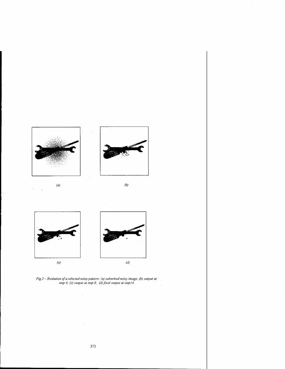
(a) (b)

(c) (d)

Fig.2 - Evolution of a selected noisy pattern: (a) submitted noisy image; (b) output at' step 4; (c) output at step 8; (d) final output at step!4.

373

2000 6™ IEEE International Workshop on Cellular Neural Networks and Their Applications Proceedings

The Longitudinal Motion Stereo Problem: a CNN Approach

Sergio Taraglio, Andrea Zanela, Antonio Pellecchia

ENEA, C.R. Casaccia Via Anguillarese, 301, Rome, 1-00060, Italy

Ph:+39 06 30486190 Taraglio, b 121 .zanela@casaccia.enea.it

ABSTRACT: A CNN based approach to the resolution of the longitudinal motion stereo vision problem is presented. Because of the geometry of the system, through the use of a reference transform in the image sequence, the correlation of pixels between image frames can be performed with a static stereo vision algorithm, the Stereo-CNN. Results on real images are presented.

1. Introduction

There are many different approaches to retrieve three dimensional information from images. For example the static stereo vision problem, where from a left and a right image it is possible to compute the spatial position of the objects of the scene. A different strategy is to use a single TV camera and move it in some known way, it is thus possible to retrieve the spatial information on the grounds of the different projection of the objects in the different frames [1]. To this class of algorithms belongs the so called longitudinal motion stereo problem and the lateral motion stereo problem. In the first the camera is made move towards the scene, while in the second it is made move laterally.

The first problem can be considered a special case of the broader problem known as the optical flow. In the longitudinal motion stereo problem we are interested in analysing the scene on the grounds of an image sequence, in which the camera moves towards the scene on a straight line, parallel to the optical axis. In the optical flow, instead, the motion can be totally general and the resolution of the problem implies the discovery of the motion vectors of all the pixels in the image.

The standard algorithm used for the problem implies the two dimensional correlation of pixels. It is necessary to understand where a given object has moved from one frame to a subsequent one. Since the object will have undergone a displacement in both the x and the y axis, the correlation ought to be two dimensional. The underlining standard assumption is that the objects in the image have not changed their sizes in a detectable way, i.e. that the frames are near.

In the following a CNN [2] based algorithm for the resolution of the longitudinal motion stereo problem will be presented. The main philosophy of the approach is that of reducing the dimensionality of the problem to a smaller one. In this way it will be possible to employ an existing algorithm for this new problem.

The key point of this work is represented by the feasibility of a hardware implementation of the CNN at the base of the algorithm; this, in turn, will allow real time performances [3],

The presented algorithm will firnish further information on the spatial structure of the environment that will be fused with that coming from the standard stereoscopic algorithm in order to obtain more reliable data for the autonomous navigation of robots, see for example [4][5].

In section 2 the longitudinal motion stereo problem is discussed. The possibility to lower the problem dimension is presented. In the third section is briefly reviewed the variational approach to the stereo matching problem, with the implementation of a neural based minimisation. In section 4 are shown some experimental results and finally in the fifth section the conclusions of this work can be found.

2. The Longitudinal Stereo Motion Problem

Longitudinal motion stereo infers depth information from a forward or backward motion of a single camera, and, consequently, can be extremely useful in autonomous robot navigation applications, e.g. the time-to-impact computation.

For the sake of simplicity in the following it is assumed that the camera moves forward along its optical axis and that the origin of the image plane coordinate system is at the centre of the image. In such a way the FOE (Focus Of Expansion) of the motion is coincident with the centre of the image. The velocity of the camera is assumed to be constant and known, see Figure 1.

The standard algorithm used to solve this kind of problem implies the two dimensional correlation of pixels. It is necessary to understand where a given object has moved from one frame to a following one. Since the object will have

0-7803-6344-2/00/S10.00 ©2000 IEEE 375

undergone a displacement in both the x and the y axis, the correlation ought to be two dimensional. Referring to Figure 1, the above means that the problem is to properly match point PO in the first image with PI in a subsequent frame.

ObsP) ^

PO »

0 x

pi y,

0 *

imgO •img1

Figure J. The geometry of the system. The observer moves with velocity v along the optical axis, taking the two images imgO and imgl.

But there is an evident symmetry in the outlined geometrical arrangement, the epipolar lines in this motion problem are all radial, in other words the objects, due to the geometrical set up chosen, will move all in a radial way. This observation opens the way for a reduction in the problem dimension. Naturally this decrease in the problem dimension is not true, the symmetry individuated only helps in the discovery of the true dimensionality of the problem. A similar idea can be found in [6], where the use of a retina like CCD sensor is foreseen for the broader problem of space variant active vision.

Let us consider a transformation of the reference frame in the input images. Let us move from a standard two dimensional linear reference to a polar representation. Let us assume that the origin of this coordinate system is still in the centre of the image, i.e. the FOE. In the polar frame representation the epipolar lines will automatically be parallel to one of the axis. In Figure 2 an example of this transformation is presented, on the left the original image with the polar grid superimposed and on the right the polar representation. Here the radiuses are parallel to the horizontal axis and the different angles are on the vertical one. In the right image are clearly viewable the comers of the original image.

With this simple reference transformation the true dimensionality of the problem has been retrieved. The correlation to be performed will now only be along the radius direction, independently for each angle. In other words the longitudinal stereo motion problem has been reduced to a standard static stereo vision problem, i.e. a mono dimensional correlation along the epipolar lines. It is now sufficient to retrieve the radial shift that each pixel in the image has undergone. The approach here employed is based on a CNN and makes use of the Stereo-CNN algorithm [7].

3. The Stereo-CNN Algorithm

The process of matching the conjugate points, either in the standard stereo correspondence or in the radial motion here considered, can be performed by algorithms capable to yield dense disparity maps through the simultaneous solution of the matching problem for all the image pixels. These algorithms try to compute the disparity function via the minimisation on the whole image of an energy functional representing the problem. As it is well known, the stereo matching problem is inherently an ill posed one. The main issue being that of the occluded pixels, i.e. those pixels belonging to objects which are seen in one of the two input images, but not visible in the other. The situation for the radial motion matching is entirely the same. But the regularisation of the problem is possible through the use of a variational approach under some restrictive hypotheses such as the absence of occluded pixels and a smoothing term in the energy function in order to produce a small disparity gradient [8]. The various variational algorithms described in the literature on the stereo matching problem differ one another in the way in which are chosen the functional to be minimised and the procedure through which the energy is minimised.

376

üBBBBI

- JBBBI

1»v lil . ""«ft*«

. . . .'..«MMani ,"**-» "SiiBBBJ

ÜU ^gaffiffia«!

Figure 2. The polar transformation of an image. Left: the original image with the polar grid superimposed. Right: the polar representation; the radial coordinate is along the x axis and angular is on the vertical one.

The existence of a Lyapunov function allows the possibility to utilise a CNN as an optimising tool in order to solve a problem expressed in a variational form and thus to handle the stereo vision problem [7]. Through the comparison of the energy expression of the stereo matching problem, as coded via a CNN, and its internal energy function, the three dimensional Lyapunov function, it is possible to derive the connection templates that specialise a general purpose CNN to this application.

In order to use the Stereo-CNN algorithm to retrieve depth information in the longitudinal motion stereo problem it is necessary to follow the following steps.

First an Euclidean to Polar reference transformation in the frames of the video sequence which are to be used must be performed. Once that the two images are in the polar representation it is possible to utilise the Stereo-CNN algorithm to retrieve the radial disparity of the pixels in the image. From the retrieved disparity it is possible to compute both the optical flow and the spatial position of the pixels. The information on the optical flow are directly furnished by the disparity map produced by the network. The spatial information is derived through simple geometry considerations on Figure 1 through the equations:

Z-4fl.-rf (1) D

where Z is the distance of the pixel seen in the second image at a radial distance of p,, with a disparity of D and d is the

distance travelled by the camera between the grabbing of the two frames. From equation (1) it is possible to retrieve the other two spatial coordinates with the:

X = R0cos&l;Y = R0sini% (2)

where R0 = Zpx /f is the actual distance from the optical axis of the object at distance Z seen at the image radial

coordinate of p,, with a camera of focal length/and t? the angular one.

Naturally the reliability of the estimates is a function of the correctness of the assumption of a perfectly centred FOE. Besides the more reliable pixel disparities are those relative to a position in the image which is not too central and not too lateral. This is due to the chosen geometry: in the limit the central pixel will possess an always null motion disparity since is the FOE; the outmost pixels, instead, will always be occluded, being even not any more present in the second of the two frames out of the camera movement. In order to render denser the image portion where disparity values are reliable it is possible to consider a different experimental geometry in which the FOE may even be off image, naturally the opportune polar transformation must be performed.

The presented approach, naturally, works under the assumption that the movement undergone by the camera is not too large. Under this restrictive assumption the pixels representing an object are thought not to change in number and to move only in a radial way. If the movement of the camera becomes too large, a given object may become larger in the second frame due to its nearing to the camera. In this case the pixels of the object may move also in the angular direction, creating false matches or pixels for which no radial matching is possible.

The interest for such a problem is evident in the field of autonomous robotics and is further strengthened by the existence of an hardware implementation of the Stereo-CNN algorithm, presented in this Conference in other works [3][9]. The typical convergence time of this CNN hardware board allows in the overall a performance of about 10 frame/s. This figure may represent the feasibility of an implementation for the longitudinal motion stereo problem with near real time performances.

377

4. Experimental Results

In the following are presented some experimental results on the longitudinal motion stereo vision problem. In Figure 3 is presented a test case consisting of a sequence of a newspaper patterned wall. The sequence is

composed of several frames of 128 by 128 pixels with depth 8 bit. In the Figure can be found the full flow of the algorithm. Beginning from one of the input images, the relative polar transformation which is fed to the Stereo-CNN algorithm. The resulting polar disparity map is shown together with the obtained ground map. This map is obtained through the equations (1) and (2) from the disparity map. The wall shape is reconstructed, apart from a false obstacle due to the upper right white patch in the disparity image. As above said the more reliable information in this algorithm comes from the intermediate pixels between the central and the lateral ones.

Figure 3. Wall test example. Upper left: one of the images of the sequence. Upper right: the polar transformation of the image. Lower left: the polar output disparity map. Lower right: the reconstructed ground map.

In Figure 4 is presented a different example where it is retrieved the velocity of the pixels in a sequence of frames of a set of nuts. As in the previous figure one image of the sequence is displayed together with its polar transformation. The second row basically shows the same information. On the left the polar disparity map and on the right the input image with superimposed the pixel velocity vector field. The magnitude of the velocity is proportional to the vector length.

Since the camera is axially moved towards the scene, the overall behaviour of the pixel will present a velocity radially increasing. If an object is nearer, it will possess a larger velocity than the background. It is interesting to note in the last image how the system is able to find such a behaviour. It is evident how the velocity vectors arc smaller in the upper right corner, the background, as confronted to the ones in the lower left corner, pertaining to some of the nuts which are in the foreground.

5. Conclusions

A CNN based approach to the problem of recovering information from image sequences has been presented. The problem addressed is that of the longitudinal motion stereo vision.

Through an appropriate coordinate transformation the true dimensionality of the problem has been unveiled, opening the way for the use of the Stereo-CNN algorithm. This algorithm solves with a multilayer CNN the classical stereo vision problem, i.e. matches conjugate points along the images epipolar lines.

378

The results here presented are to be considered preliminary. Much work has yet to be done, especially to properly take into account all the problems relative to the coordinate transformation which warps the pixel shape. Nevertheless these results show that the underlining idea is correct and, possibly, fruitful especially in the field of autonomous robotics.

Besides the proposed approach will straightforwardly benefit from the feasibility of a hardware implementation of the CNN at the base of the algorithm [3][9], opening the way for the acquisition of further information on the environment in which the robotic platform operates.

Figure 4. Nuts test example. Upper left: one of the images of the sequence. Upper right: the polar transformation of the image. Lower left: the polar output disparity map. Lower right: the reconstructed pixel velocity field.

References

[1] U.R. Dhond, J.K. Aggarwal, "Structure from Stereo - A Review", IEEE Transaction on systems, man, and cybernetics Vol. 19, pp. 1489-1510,1989.

[2] L.O. Chua, Y. Yang, "Cellular Neural Network: Theory", IEEE Transaction on circuits and systems Vol. 35, pp. 1257-1272,1988.

[3] M. Salerno, F. Sargeni, V. Buonaiuto, S. Taraglio, A. Zanela, "Preliminary testing of a board for CNN based stereo vision", this Conference.

[4] A. Zanela, S. Taraglio, "A CNN Stereo vision system for autonomous robot navigation", this Conference. [5] A. K. Dalmia, M. Trivedi, "Depth extraction using a single moving camera: an integration of depth from motion

and depth from stereo", Machine Vision and Applications Vol. 9 pp 43-55,1996. [6] M. Balsi, "Focal-plane optical flow computation by foveated CNNs", Proceedings of the Fifth IEEE Int'l

Workshop on Cellular Neural Networks and their Applications, CNNA-98, London, U.K., pp 149-154,1998. [7] A. Zanela, S. Taraglio, "Sensing the third dimension in stereo vision systems: a cellular neural networks

approach", Engineering Applications of Artificial Intelligence, Vol. 11, pp. 203-213,1998. [8] T. Poggio, V. Torre, C. Koch, "Computational vision and regularization theory", Nature Vol. 317, pp. 314-319,

1985. [9] M. Salerno, F. Sargeni, V. Buonaiuto, "The design of a new CNN chip for stereo vision", this Conference.

379

2000 6™ IEEE International Workshop on Cellular Neural Networks and Their Applications Proceedings

Genetic programming of a CNN multi-template tree for automatic generation of analogic algorithms.

V. M. Preciado, D. Guinea, J. Vicente, M. C. Garcia-Alegre and A. Ribeiro.

Institute de Automatica Industrial- Spanish Council for Scientific Research La Poveda (Arganda del Rey) - 28500 Madrid, Spain, preciado@iai.csic.es

ABSTRACT: A fruitful field into the CNN research is being the development of analogic algorithms utilizing combinations of single templates to perform complex image processing tasks dedicated to industrial applications, vision problems in robotics, pattern analysis, etc. In this work a software implementation for the automatic generation of analogic algorithms by mean of a genetic search is presented. First, we are going to shortly present an improved automatic templates generation, task already solved in before works. Next, an algorithm for generating templates in cascade will be showed like the natural and original extension of the already known tool. Lastly, the multi-template tree concept derived from the AI field is applied in the automatic generation of analog algorithms, and its solution based in both genetic- evolutionary search and heuristic methods are exposed.

1. Introduction

The traditional image processing techniques require a lot of computational effort due to data on each pixel are computed in a sequential way and the path of information is an A/D converter. The delay accumulation create in this process is unacceptable in real time image processing because of the information flow managed in the usual vision tasks (e.g. automatic industrial inspection, vision problems in robotics, pattern analysis, etc.).

Thus, the use of a massive parallel architecture working with analog signals avoid the previous problems. Thus, it is important the development of analog algorithm to perform complex image processing tasks dedicated to many different fields.

1.1 Cellular Neural Network Model

The basis idea of Cellular Neural Network (CNN's) is based on an array of analogic dynamic processors which cells interact directly within a finite local neighborhood [1]. The local CNN connectivity allow its realization as VLSI chips that can operate at a very high speed and complexity[2].

The dynamic of the array is defined by the following system of differential equations:

"' Cel{kl)eNr(ij) CW(W)E/Vr(y) vU

taking into account that:

Nr(iJ) = !f(k,l^max\k-i\,\l-j\}<r}

where ij refers to a grid point associated with a cell on the 2-D grid, and k I is a grid point in the neighborhood within a radius r of the cell ij. Equation (1) describes a nonlinear dynamical system due to the equation (2) that includes in our system a piecewise linear function of saturation. In the equation (3) the concept of neighborhood is defined.

In many applications, the cloning templates A, B and the threshold current I are translation invariant. In this case, the dynamic of the array can be described by:

0-7803-6344-2/00/S10.00 ©2000 IEEE 381

C-^- = -R,Vxu{t)+ I>„(V')+ Z^^+Z W

When the template is space-invariant each cell is described by a simple identical cloning template defined by two (2r+l)x(2r+l) real matrices, as well as the constant term /.

As the network will be devoted to this kind of tasks, it is convenient to represent equation (1) by the approximation of a difference equation of the form :

^,[« + J] = '/,,,[»] + 7(-^,,['<]+ YtA(i,j;k,l)Vtk,[n]+ J,B(iJ-Xl)-VM+l) (5) (- " <'(A./)e,V, (:./) ('(A./kMM)

where h is the time step used to compute each iteration in a Runge-Kutta 4 integration process, A and B are the cloning templates.

2. Single-Template Automatic Generation

Nowadays CNN architectures implemented as VLSI chips shows the aptitude of extremely high speed compared with traditional digital image processing tools. The proliferation of more and more sophisticated CNN architectures, and the increasing effort to implant practical system for industrial applications based in CNN chips, make necessary the programming of software development tools for template design.

This work presents a CNN simulator with the feature of automatic template generation, like other simulators developed in previous works[3][4], from training examples by mean of a Genetic Algorithm. The simulator processes an input image from an initial state, and using a certain template, it produce an output image performing a particular image processing operation. With the extra feature of automatic template generation the process is inverted, so that, with an input image and the desired output image, the genetic algorithm is able to search a template that perform that operation. The discrete search space and the nonlinearity of the fitness make Genetic Algorithm (GA) a good candidate for this optimization task.

2.1. Search Space

The number of parameters in a whole template set (neighborhood within a radius r=\) is 19. Taking into account that analog VLSI chips have a certain template parameters accuracy, 8 bits are utilized to encode each template parameter. So the chromosome length utilized to encode the template parameters is 152 bits (19 parameters x 8 bits/parameters).

This chromosome length can be drastically reduced in the case that the image processing task have a symmetric behavior (e.g. border detection, averaging, halftoning etc.). Thus, under symmetric behavior the cloning template is reduced to 7 representative parameters (3 parameters for each matrix and another one for the bias current), and the chromosome is a 56- bits string.

The speed of convergence in the algorithm rely on the options set selected and the genetic operators values. The options that can be changed in the program are the following: Crossover probability, Mutation rate, Population size and Transient options. Besides, the developed program allows to adjust the number of generations for the algorithm to converge, and also the number of necessary steps to have a good approximation of the difference equation (5).

This algorithm must search the template that minimize an energy function proportional to the to the difference between pixels from the current output image and the desired one.

2.2. A Simple Application Example of Automatic Templates Generation

The appearance of the program screen is showed below. In the example the genetic algorithm has been used to search a templates able to perform a simple border detection with only 10 iterations.

This software has been programmed in OOP with visual components under Borland C++ Builder programming language, in this way we have improved the GUI of previous works about this same task.

382

■ -IJIXI

INPUl IMAüt

Iterations [iö

Slot Slap

CURRENT 0UTPU1 DES1RE0 OUTPUT

Iteration number: 10

531624 [

OMStMCoKUimr

StepWdth

Error

W Simstric

tenplrcOopraKvr

~ I Pondati«. SKB 'SO I

J Sriecfai Encodng

UaierUrJ pMÖÖ" ^ lowerlimt j.inrao ""V

39 I -30391 39 I -5M3 [ «823 j -58ttj

AMOT- "*l . OTÄOÄ laa> I

y-Vg. 2. Automatic template generation program screen.

3. Cascade-Templates Automatic Generation

Going beyond, there is many advanced applications with CNN's where several templates are working consecutively for a concrete purpose. In this case the information to encode is the 19 parameters of each stage and two images (input and initial states). This new application is the natural and original extension of the already known tool.

The way it has been done is by a first stage with input image equal to the image to process, and an initial state selected from a fixed set of initial states. This initial states has been selected from numerous samples of simple templates, concluding that almost all the initial states are including in a reduced collection of images (the input one, white, black and grey scale, etc.)

3.1. Search Space and its reduction

Thus, the number of bits needed for encoding each stage in a cascade-template case are the same than in the single- template case plus 8 bits needed for encoding both input and initial images number (4 bits for encoding each image number from the collection. The search space for the genetic search is Nx( 152+8) bits in the general case, being N the number of stages.

We can drastically reduce the dimension of this cube if the symmetric condition is utilized, obtaining a search space of Nx(56+8) bits. However, the search space is too big for assuring the convergent of the evolutionary process. So, a heuristic method has to be used to make the search well-conditioned for the algorithm to perform. This consist in the use of a library of well-known templates like initial parameters of each stage.

383

4. Multi-template tree and Genetic Programming

In this part of the work, a general methodology for developing a general case of analogic algorithms utilizing combinations of single templates to perform complex image processing tasks is presented. In this way the last possible step in the evolution of the process complexity has been done. Some concepts in this section are related with AI theory, in such a way that in this work we are in the intersection field of AI and Image Processing by CNN.

4.1. Notation and Representation of the Tree

The situation is that each template can be seen like an operator which acts directly on two images, and this can b e represented exactly by a diagram of the type called tree:

Initial Stale Collection A

Tree node configuration

Tree example

Fig. 3. Tree and node example.

4.2. Search Space and its Reduction by mean of an Heuristic Method

The representation in the machine can be done by constructing a table in which all variables (images) and operators (template) are listed. For each symbol we give three items of information: operator and two variables represented like (S,L,R).

In any case L and R can themselves be trees; that is, these variables can be a pointer to another operator in the table, that is, indices showing where in the table these are to be found, and therefore the relevant operators. The terminal symbols of the tree are the variables and constants of the expression and have no L, shown by setting L=0.

Once the tree has been encoding we must performance the genetic search for self-programming the analog algorithm. In this case we start in a library of well-known templates and a collection of initial states. In this way we have search an algorithm able to self-programme.

In conclusion, an evolution of the automatic generation of solutions by mean of genetic algorithms has been showed, being both cascade-templates and tree-templates original extensions of the automatic generation of templates. Some industrial applications of this algorithms are being developed (Automatic defects detection in eggshell and metal laminates) to try make CNN an usual visual system in real problems.

384

5. References

[1] L. O. Chua, L. Yang. "Cellular Neural Networks: Theory". IEEE Trans, on Circuits and Systems. Vol. 35, No. 10. pp. 1257-1272. October 1988.

[2] S. Espejo, R. Carmona, R. Dominguez-Castro, A. Rodriguez-Vazquez, "A VLSI oriented continuous-time CNN model", Int. Journ. Of Circuit Theory and Applications, vol. 24, pp. 341-356 (1996).

[3] R. Caponetto, M. Lavorgna, A. Martinez and L. Occhipinti, "Cellular Neural Network Simulator for Image Processing Applications", 1998 Fifth IEEE International Workshop on Cellular Neural Network and Their Applications Proceedings, pp.360-365. April 1998.

[4] Martin Hanggi and George S. Mostchytz, "Stochastic and Hybrid Approaches Toward Robust Templates", 1998 Fifth IEEE International Workshop on Cellular Neural Network and Their Applications Proceedings, pp.366-371. April 1998.

385

2000 6™ IEEE International Workshop on Cellular Neural Networks and Their Applications Proceedings

On the Rectangular Grid Representation of General CNN Networks

Andräs G. Radvänyi

Analogical and Neural Computing Laboratory Computer and Automation Institute of the Hungarian Academy of Sciences

P.O.B 63, Budapest, H-1502, Hungary, FAX: (+36) 1 2095264 E-mail: radvanyi@sztaki.hu

ABSTRACT: Although the cellular neural paradigm in its original form provides a suit- able framework for investigating problems defined on arbitrary regular grids, the chips - ready ones or under design - as well as the available simulators are all restricted to a rectangular structure. It is not at all self-evident, however, that the rectangular structure is the most suitable to represent every practical problems. In this paper we demonstrate that several CNNs of various regular grids can be mapped onto the typical eight-neighbour rectangular one, by applying weight matrices of periodic space-variance. By adopting this option, the applicability of cellular neural chips and simulators can be extended to investigate problems of essentially arbitrary grid structures.

1. Introduction

In introductory publications [1] the cellular neural network is defined as an array of uniform elementary processors operating in the nodes of some regular grids. Although in [2] regular triangular, rectangular and hex- agonal grids were distinctly mentioned, the CNN theory and practice have dealt almost exclusively with CNNs working on rectangular grids since then. The simulators developed for experimenting with CNNs are based exclusively on rectangular grids. The weight matrices (templates) are denoted by rectangular matrices, as well. Also the chips, realised so far or still in design phase, are all of this sort. It is not at all obvious, however, that the rectangular grid is the most suitable one to represent all practical problems; the optimum grid structure stems always from the internal dependencies of each specific problem. The general spread of the rectangular grid is mainly due to the rectangular matrix notation used in CNN and also to the fact that array type elements in programming languages of software simulators and the row-column organisation of data in graphical hardware devices are, in effect, also rectangular matrices.

In the following, we demonstrate that by applying space variant weight matrices the chips and simulators with rectangular grid, in a great number of cases, can be used to solve problems that are defined in other types of grids. Since we cannot propose a general method, we investigate numerous regular planar grids with cellular weights and show how to map them onto rectangular grids and how to find the corresponding weights. As for non-unique mappings, we also suggest criteria for the best choice. In addition, as counter examples, we show grids that cannot be mapped onto a rectangular grid.

2. Regular Planar Grids

The operation of a cellular neural network is basically determined by the weighted interconnections of its nodal processors, which is defined by weight matrix Q. For the sake of simplicity, we consider the system of interconnections in the initial network to be homogeneous, even if the network consists of several different types of nodal processors with different number of connections in different directions. In a homogeneous system of interconnections the connection weight between any two adjacent processors is determined by the geometrical direction of connection alone, independent of the type of processors. The different directions will be identified by a mix of points of the compass and the dial. (It is worth noting that considering a homogeneous system of connections means only a simplification in notation; on the basis of its results, mapping inhomogeneous connections from the same grid can easily be performed.)

The regular rectangular grid is what simulators can work with. Since the allowable radius of neighbourhood varies, here we suppose the simplest rectangular grid in which each processor is connected to its eight adjacent neighbours; in most cases this will answer our purpose. (Later we will see, however, that the possibility to connect more distant processors to each other in a rectangular grid provides the possibility for the simulation of multi-layer structures in a single layer grid.)

As it is well-known, considering congruent polygons alone, the regular triangular, rectangular and hexagonal grids are the only regular contiguous tesselations of the plane. Taking into account, however, non-regular congruent polygons too, several further tesselations can be conceived. Another group of tesselations can be composed by using two or more types of regular polygons as building components. For our investigations the theory of plane ornamental groups, a branch of geometry, provides sufficient number of initial grids: the whole

0-7803-6344-2/00/S10.00 ©2000 IEEE 387

set of tesselations that can be obtained from the regular vertex grid through discrete geometrical transformations, rotations and translations [3,4,5]. To ornamental groups belong the rosette, the frieze and the wall-pattern groups. The rosette groups are free of translations, they contain nothing but discrete rotations. With additional unidirected translations and their inverses we obtain seven frieze groups. Finally, we have 17 wall-pattern groups, called also plane crystallographic groups, containing more than one non-parallel translation, which cover the whole plane without interstices with finite unit cells.

It is noteworthy that many of the ornamental groups can be recognised in ancient Egyptian and Chinese decorations. All 17 of the wall-pattern groups were known empirically to the Moors, as shown by the ornaments decorating the walls of the Alhambra in Granada, that was built in the 13th century. The first complete enumera- tion of the finite ornamental groups is ascribed to Leonardo da Vinci.

To demonstrate our present message, those 19 regular grids obtained as contour nets of wall-pattern groups and their duals are more than enough. (Their total number is less than 2*17, partly because some of the groups differ only in the emplacement of their constituent unit cells and have the same contour nets, and partly because some of the contour nets are either self-dual or dual in couples.)

It follows from the generation rules of wall-pattern groups that in a tesselation each node has the same rank and each node is surrounded by the same set of regular polygons. The groups are identified by the list of composing polygons: T(n,,n2,..,nk), where k is the nodal rank and n, is the number of edges of the i-th polygon. Following from the concept of duality, a dual tesselation consists of congruent k-angles and is denoted by DOiijihvtnit), the list of ni nodal ranks of its composing k-angle. E.g., the hexagonal grid is denoted by T(6,6,6), for - as shown in Figure 2 - it contains tertiary nodes all surrounded by three hexagons. Its dual is the triangular grid denoted by D(6,6,6), the same list as before, meaning that the rank of each vertex in the composing triangles is six. On the other hand, each node in a triangular grid is surrounded by six triangles, therefore it can be denoted by T(3,3,3,3,3,3) as well, and thus we conclude that D(6,6,6) = T(3,3,3,3,3,3). Since duality is valid vice versa, the hexagonal grid can be considered and denoted as the dual of the triangular one, therefore T(6,6,6) = D(3,3,3,3,3,3), too.

3. The Graph-Theoretical Formulation

Considering the discussed problem from the view of graph-theory, we have to find homomorphic * map- pings between coloured graphs. The colouring can be used to represent weight matrices and by requiring a minimum number of colours, criteria can be defined to compare and evaluate alternative mappings. In the following, we perform the task in two steps without colouring: first the mapping of graphs will be determined and next weights will be attached to the edges.

Let the graph of the initial tesselation - that will be planar, without loss of generality, in all investigated cases - be denoted by G = ( V, E ), where V is the set of vertices and E is the set of edges. The graph of the resulting rectangular grid is G = ( V, E), a section of which is shown in Figure 1. Since this is not a planar graph, in order to distinguish crossings from vertices, the latter ones are marked by circles.

The homomorphic mapping 9 : G -» G that we seek for is composed of the *v '• V -» V mapping of vertices and the *E: E -> E mapping of edges, i.e. 9 = (#v > *E)- It determines a subgraph in G which is isomorphic with G. Since the initial graph G does not contain multiple edges, the mapping 9y of vertices uniquely determines the mapping #E of edges. For practical reasons it is advantageous if the mapping 9\ of vertices is an isomorphy, i.e. there is a one-to- one correspondence between the vertices of the two graphs. (In this case, for lgure ' " -neig our instance, the computer memory that is available for a simulator can be wholly rectangular grid U exploited.)

In the theory of algorithms, subgraph isomorphy is considered among the hard problems that cannot be solved in polynomial order, in general [6]. Therefore, we cannot provide general criteria for the existence of a subgraph in G which is isomorphic with G, i.e. criteria to decide whether the initial grid can be represented in a rectangular grid or not. However, since the rank of vertices in the rectangular grid is eight, it is obvious that no rectangular grid representation exists for initial grids with vertices of rank higher than eight. For example, the dual grid D(12,6,4) in Figure 2 has no rectangular grid representation.

The grids investigated and their rectangular representations are shown in Figure 2. One of the wall-pattern groups, namely T(12,12,3), together with its dual were left out of investigations, partly because it can be considered as a "loose" variant of T(6,3,6,3) and because, owing to the rank-constraint, its dual D(12,123) cannot have a rectangular mapping. Notwithstanding, three such grids were included for which we could not find a rectangular isomorph. In addition to the above-mentioned D(12,6,4), we cannot represent D(6,4,3,4) and D(6,3,3,3,3) on a rectangular grid, however, we cannot simply prove that no such representation exists. In the

388

T(3,3,3,3,3,3) = D(6,6,6) T(4,4,4,4) D(4,4,4,4)

■f^r -f^- \ / \ / \ / \ / \ / \ / \ / \ / ^- ̂ ^

T(6,6,6) = D(3,3,3,3,3,3)

s < ±kL

< v/

s/ \ \ / \ \ /^ \ \ \

'\ \ / \ \ / \A \ \ \

v\ 4^ \ 4^ \/ T(6,3,3,3,3)

T(6,3,6,3)

\ <- \ <- \ \ / / /

\ \ \ s / / /

\ \ \ \ .... / / / ̂

T(4,3,4,3,3)

'/, <//, V , V // / /, V

y/, '//, V / N\ w \ v s-

<>/ '// '/ , '/ // / /< '/ - r \ \ ^ r-

s 's ■ s

T(4,4,3,3,3)

T(8,8,4)

\\ // \\ // 1 1 1

-V w // \\ II II

\\ // \\ // 1 1 1 // \\ // \\

D(6,3,3,3,3)

D(6,3,6,3)

D(6,4,3,4)

itctct * /_■_

"// / __

-// —// A A \

'. VvVVrv /

/.

D(4,3,4,3,3)

x\\\\\\\^

xSSrNv D(4,4,3,3,3)

'////////

T(12,6,4) D(12,6,4)

Figure 2: Regular planar grids and their rectangular representations

389

case of D(6,4,3,4), such "long, closely running paths" can be found inside the grid, the length difference of which increases proportionally with their overall length. This feature can substantiate the hypothesis that no isomorphy can be established between the two graphs.

Wide stripes of grid D(6,3,3,3,3) of "daisy" pattern (Figure 3-a.) - friezes of daisy pairs - have rectangular isomorph; a fact which gives a hint that nei- ther in this case can a simple local criterion for the existence of isomorphy be found. A single daisy of discrete rotational symmetry is isomorphic in a rectangular grid to a bird of reflectional symmetry (Figure 3-b.). Furthermore, it can be shown that a slight alteration of D(6,3,3,3,3), an insertion of hexagons sparsely into its pentagonal structure, results in a grid of which a rectangular representation will exist (Figure 4.).

a.) b.) Figure 3: "Daisy" and "bird" patterns in grid D(6,3,3,3,3)

Figure 4: Mapping of the modified D(6,3,3,3,3) grid into a rectangular one

4. Weight Matrices In Rectangular Grids

4.1 Notations

In the initial grids, homogeneous weights are considered, i.e. each weight is determined by the direction of the corresponding edge by itself. In the investigated grids, in addition to the horizontal and vertical ones, edges slanting at 30, 45 and 60 degrees to the horizontal direction appear, i.e. on the whole, edges from 16 different directions may connect to a vertex. (We do not consider as separate cases those isomorphic ones obtained by rotating the investigated grids.) For enabling simple identification, the weights of the 16 possible directions and the "self-feedback" are denoted as shown by the two composite weight matrices in Figure 5. With its indexing and arrangement suggesting a dial, weight matrix QD can denote 12 connecting directions in 30 degree steps. Weight matrix Qc adopting its subscripts from the compass can mark eight directions in 45 degree steps. (The notations of horizontal and vertical directions are redundant, they appear in both matrices.)

In any single weight matrix only those [~ Q Qw ^n ßoi

ßlO ß>2 ß()9 Qo Ö03 ßo8_ _ ß)4

weights are to appear that belong to an exist- ing edge in the corresponding grid, i.e. (in addition to the weight of the self-feedback) QD

=

the number of entries in a weight matrix is equal to the number of neighbours which a processor in the grid is connected to.

ßo7 ß06 Qo:

Qc =

QNW QN Qm

Qw Qo QE

isw Qs Qi ■SE

4.2 Mapping criteria Figure 5: Direction dependent notation of weights: dial and compass

In some cases, as show in Figure 2., there are more than one way to represent a regular grid in a rectangular one. For such cases the version best suiting the related task is to be chosen. Two fundamental criteria are worth pondering: i.) The number of weight matrices required in the possible variants usually differs. The variant with the least number of weight matrices is most probably the best choice. The question, whether the number of weight matrices is a crucial point or not, highly depends on the options of the applied device, chip or simulator: beside the maximum allowable number of weights, the loading time of weights is to be considered as well,

ii.) A significant point for consideration can be the best utilisation of available processors or the available mem- ory, in the case of simulators. As always in practice, using finite grids and starting from the same initial window, the different variants may result in outcoming segments of different shapes, therefore the dead processor area at the borders may be different as well. Furthermore, there exist also sparse mappings with embedded dead proces- sors. In both cases, different numbers of processors can be mapped by the different variants onto the available rectangular grid area.

In experience, the above two criteria are contradictory: the rectangular processor area typical in CNN devices can be utilised the best by mappings having several weight matrices.

390

4.3 Weight matrices in general grids

In the following, samples of weight matrices belonging to the investigated grids are tabulated. In addition, each table shows a magnified segment of the corresponding initial grid and that of its rectangular mapping. The equivalent nodes in the initial grid and its mapping are denoted by the same letters which are to identify the corresponding weight matrices as well. Composite matrices of these letters show space-variance of weight matrices in the rectangular grid. In the initial grids, dotted lines are to mark paths that are mapped onto horizontal or vertical lines of rectangular the grids. (In the case of mapping variants, several such lines may appear in the figure.)

5. Conclusions

With numerous regular grid structures, we have demonstrated that by applying space-variant weight matrices, a CNN of rectangular grid, on-chip or simulated, can represent several regular non-rectangular CNN structures. The same way, the method can obviously be extended to non-regular structures as well. The allowable variety is limited only by the maximum number of simultaneously active weight matrices.

Since the applied 8-neighbour rectangular grid itself is not a planar graph, it can represent CNNs of non- planar structure as well. For instance, the two-layer CNN of cubic grid in Figure 6 has evidently got its rec- tangular grid equivalent shown in Figure 7-a, requiring two distinct weight matrices to represent the initial in- layer and inter-layer connections.

a.) b.) Figure 6: Spatial, two-layer cubic grid Figure 7: Single layer representations of the cubic grid

So far we restricted our scope to rectangular CNN structures in which each processor is connected only to its eight closest neighbours. By extending inter-processor connections to farther neighbours, even one single rectangular CNN layer can represent more elaborate spatial, crystal-like structures. Figure 7-b is to illustrate this concept, showing an alternative representation of the two-layer cubic grid of Figure 6. In this case, the processors of rectangular grid are connected also to the second "circle" of their surroundings, resulting in a sparse mapping. However, this sparse mapping can be generalised: the more distant processors can be intercon- nected in a rectangular CNN grid, the higher is the number of spatial layers of CNN structures it can represent. The number of required weight matrices is equal to the number of initial CNN layers.

6. References

[1] L.O.Chua, L.Yang, "Cellular neural networks: Theory" and "Cellular neural networks: Applications", IEEE Transactions on Circuits and Systems, Vol.35, pp.1257-1290, 1988.

[2] T.Roska, L.O.Chua, "Cellular Neural Networks with Nonlinear and Delay-type Template Elements", Cellular Neural Networks (Ed.: T.Roska, J.Vandewalle), pp.151-161, John Wiley & Sons, 1993

[3] H.S.A/.Coxeter, W.O.J.M)ser, "Generators and Relations for Discrete Groups", Springer Verlag, 1957 [4] L.Fejes Toth, "Regular Figures", International Series of Monographs on Pure and Applied A/athematics,

Pergamon Press, 1964 [5] O.Ore, "Graphs and Their Uses", New Mathematical Library 10, Random House, New York, 1963

[6] MR.Garey, D.S.Johnson, "Computer and Intractability - A Guide to the Theory of NP Completeness", Sub- graph isomorphy, p.202 [GT48], Freeman & Co., 1979

391

Triangular grid TOMßßß) - D(6,6,6)

a. & ( Oi a.

\ \ L*N \ \ X \ \ \ \ V \ k

<>»• a, a, o ] fa, ß., o l r o a, a a. ßo ßo Q.- a» ßo a» «Ma* a. ßo o ß„a,J [ßna, oj L°a»a

Note: For case a.) one weight matrix suffices, but it results

• in a slanting window

Space variance of ooooooooooo "^ . . _. . EEEEEEEEEEE

weight malm in ooooooooooo caseb.): EEEEEEEEEEE

Qw.. -

a, i a, a.

QK,-

1RH1RW1RW

1RW1RW1RW

Qw- ßiißo, o ßo. ßo ßm fl„fl., o

QL-

0 0 L,,

U,lo 0 0 0 i„

Q.-

Ä„ 0 0

0 «OHB

«„0 0

o a, a, Q.- ßo,ßoßo

o a,ß„ r o t,, o'

Qi-U»to ° L ° u> o 0 Äu 0 '

Q.-l 0 RoK* 0 Rv, 0

Hexagonal grid T(6,6,6) ■ KWWJ)

00 &!

a. a,

Q.'

QL'

0ß„ 0 OGoßa. Oßoi 0

0 ßoi 0 ßWßo 0 0 ß«0

RLRLRLRLRL LRLRLRLRLR RLRLRLRLRL LRLRLRLRLR

■/, \\ / ,

/' l\ ■ ' /'

ß,i 0 0 ßnßoßn

ßo. ßo ß.i 0 0 ß„

IrLRIrLRIrLRl IrLRIrLRIrLRl IrLRIrLRIrLRl IrLRIrLRIrLRl

ß„a>a. ßo, 0 0

0 0 ß01* ßcßoßo,

TT&3M3)

es a, a' . es ß.A.

(* Qs e{ =° >

H \ s / s \ ̂ \ \ \ s

\ ̂ a * \ /

ABCABCABC FEDFEDFED ABCABCABC FEDFEDFED ABCABCABC FEDFEDFED

Q«-

Q.'

*=

ßi a, Qo

0,1 ß.s

a, a, a. a,

Q" a,

a. ßo a> a.

ß„ß., o 0 ß0 0

. 0 ßorßoi.

0 ß01 0 ' Qm ßo ßoi

0 ß„ 0

ßi, 0 0 ßo.ßoßoi

A A A X A A

BCBCBCBCBCB A A A A A A BCBCBCBCBCB A A A A A A BCBCBCBCBCB

Q»'

Qi'

a, a, o 0 ßo 0

ßorßo» " o a, o ß. ßo a

0 ß„ 0 a, o o ßo floß.

0 ßoi

1 0 ßo, , ßoß. „00

Iß.iß.i 1 ßo ° Iß-ß.I

1 ßoi 0

»ßoß« > ßoi 0

A A A A A A A CBCBCBCBCBCBC D D D D D D D FEFEFEFEFEFEF A A A A A A A CBCBCBCBCBCBC

QA-

a, a» o ßo. ßo ß»

0 ßoi 0 Qi-

ß„aißm ßo. ßo ßoi

0 0 0 Qc-

o a, o ßußbai o ß„ai

Qr-

a,ßo, o ß. ßo ß.l

0 ß„ 0 Qi-

0 0 0 a, ßo &! ßo. ßoi ßOI

QB-

0 ßoi 0

flo.a>a> 0 ßoißoi

Note: For case ■.) three weight matrices suffice, but it results in a slant window

fl.fl'a'aa,

a. a a, e>„ „Q- ftia.a> {a,.a,,a,a..ß„} (a.a,.a,.a..a.)

,.o».a».a,) .ßo..a»,ßo.) .&..& .ß„) .a,.a..a)

Q,

Q.-l&.a, Qc-jßo.a, QD-ißo.ß., Qt = fßo.ft Q,-(ßo.ft

F

E

-E

*

D

E / 4

B A

OA-

0 ß„ 0 ß,o ßo ßo, 0 ßoi 0

Qi-

0 ßo, 0] ß.o ßo 0 a.ß.!«J

Qc-

0 ß„ 0 0 ßoß.

Gotßo. 0 Q»-

0 ßo, 0

ß» ßo ßo. 0 ß« 0

0,- 0 ß„ ßo 0 ßißo. 0ß„ 0

0,- 0 ßnßo,

a,ßo o o ß« o

CDBEAFCDBEAF AFCDBEAFCDBE BEAFCDBEAFCD CDBEAFCDBEAF AFCDBEAFCDBE

T(6,4J,4yb

JL A t A d 0 d b

yjsOpC/v^ \=s N\ N

lüf lüf \H 5>»\ fc, N. AEAEAEAE BDBDBDBD

^® • f

7B/ f/

CfCfCfCf

/ bdbdbdbd Cy FcFcFcFc Y AEAEAEAE ■ BDBDBDBD

<j b <1 b CfCfCfCf

KÄÖO^ \)> & y \ ß„ ß« o ] r o ß„ oi

Q»- ßo.ßo 0 0 ßo, 0

Qi- ßo. ßo 0

ßmß« oj

fl.ß'a,a'a.

ft. ßo ft, a. a. ßioßn 0 0 ß„ 0

Qc- 0 ßo ° 0 ß„ß.

QB- 0 ßoß« ß»ß.i o

ftiS»äi ß,oßo, 0 ß„ß., o QA,={ßo.ß.,.ß«.ß».ß„} Qi- 0 ßoß

0 ßo, 0 » Qr- 0 ßo 0

0 ßo,ßo.

QM-(a..e-.ßoiß»ßii) 0 ßnßo o ß„ o Qc..-(ßo.ß.,.ß.,.ßm.a.) Q.- ßo.ßo 0 0.- ß»ßo 0

QB..-(ßo.ß.,.a,.ß...ß„)

Qa,-{ßb.ai.a..o».ß..j Q.-

0 ßo 0

0 ßi.ß. 0 ßo 0 «i-

0 ßoißo.

o ßi, o 0ß„ ß„

Q,.,-(ßo.ß.,.ßo.-ß..ß,) ßoißoi 0

o ß„ ß. ■i

0 ßo, ßo, J o ß„ So,

Q.- 0 ßo ßoi Oßo, 0

Qr- 0 ßo 0

ßoißo. 0

392

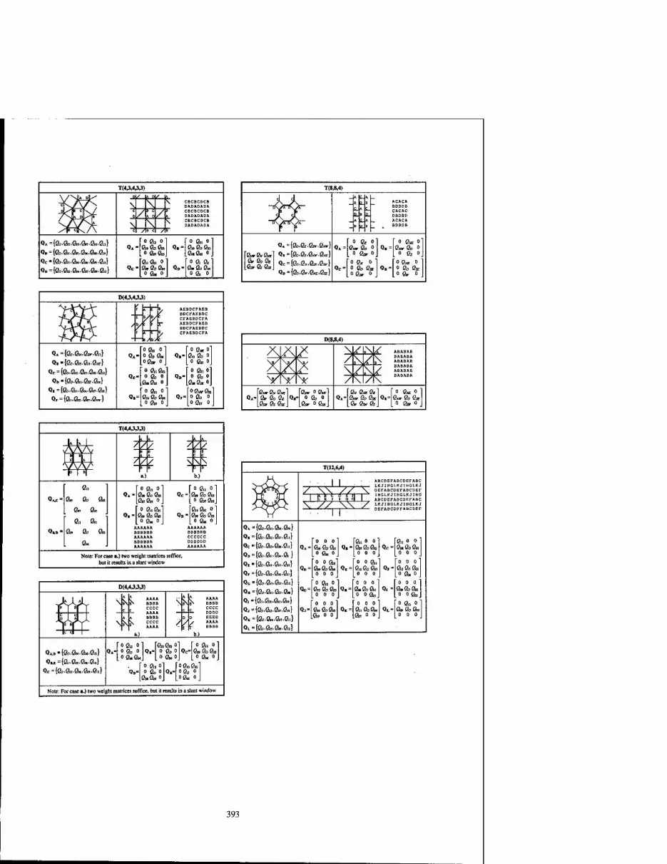
Q.={fi>.&..ft,.0«.&..0lo}

Qc={&.a..Ob4.ö».a9.0i.} OD={öo.0ra.Ö)4.ÖW,Ö»,Ö1i)

CBCBCBCB DADADADA CBCBCBCB DADADADA CBCBCBCB DADADADA

o a. o a.aa» ° ßmßa. a, a, o ß»a>a. o a< °

Q.- o a, o ßioaas ßo>ßo> 0.

o a a' &>&ß« o a o

QA= {Qo.QoQwQw}

B. 2. ACACA BDBDB CACAC DBDBD ACACA BDBDB

QA-

0 Q, 0 ßw & 0

0 &, 0 Qi-

o ß«, o ßm- a 0

o a »

Qc- o e» o o a ßss Oßar 0

Q„- °ß» o 0 ßo ßsr

.0 Qw 0

Q*-{Qb.aM.ar.ßi} Qi ={60.0,3.0.0.0^}

Qc={0o.0OT.0Oj.0Oi.0.i}

QD={0O.0O..0SE.ai}

Q<={0o.a,.Gb4.0«.0.o}

QF={öb.ßb.0O7.0w}

AEBDCFAEB BDCFAEBDC CFAEBDCFA AEBDCFAEB BDCFAEBDC CFAEBDCFA

08, » 0 aa. Oßsr 0

Qi- 0 ߻o

e,o a 0 0 ß„ 0

0 ß„a> 0 a 0

a»a» ° Q»-

0 a,» 0 a 0

ß«ßa 0

0 a, 0 ßioaa. QF-

oß™-a. 0 a 0 Oß«, 0

D(8,8,4)

A fj\ /S ABABAB

\a/ 'A

S ABABAB

/ ABABAB

\a*' NK

QA- S«irß«fi«E a ßoßi Sar ßs ßsj

Qi &» 0 ßm

0 a 0 .a» »a.

QA- ß» e«s e. s™- a a* a ß»a

Q.- ° ß» 0 1

e»»aaj 0 a» 0 J

zzz zzz

zzz SSS

ß> 1 [ 0 ft, 0 1 0 flu 0 QA- ßoifloßo Qc- a,ßoßo a a» flora, 0 0 ßora.

as 0 flnß.1 a. a, 0 QI- a>aa> Q»- a» a a» a, ig.0 0 ß« 0

AAAAAA AAAAAA a a> BBBBBB BBBBBB AAAAAA CCCCCC

a. J BBBBBB DDDDDD A AAAAA A AAAAA

Note: For case a.) two weight matrices suffice, but it results in a slant window

D(4,4A3,3>

QA.«=(a.a,.a..a,}

Ou -{&.&■.&..&,} Qc={a.a>.a>.a..ßi.}

\S\»N

\.\^

AAAA BBBB cccc AAAA

v" 1^ 1^ AAAA >INB^ BBBB

CCCC DDDD EEEE

> > J AAAA " \t f BBBB

ofl, oi raoaaoi pa, 0 QA-| O&O QB= O&O QC= Q„ QO fi*

. f 0 fl,0] \OQnQn" QD" ° Qo OQi-Oß, 0

Note: For case a.) two weight matrices suffice, but it results in a slant window

T(12,6,4)

J\ II ■ . ABCDEFABCDEFABC :w%f / \\i // ^ DEFABCDEFABCDEF *—l IktC OEM P^ IHGLKJIHGLKJIHG

1 t K J 1 H Ci 1 ABCDEFABCDEFABC ;\ // W / t-KJIHGLKJIHGLKJ —J * ■ | L ^ » *— DEFABCDEFABCDEF tyft

QA-{a>.Qu.&.Q»}

Qi={a.&j.&7.a,}

Qc'ta.ai.Om.a,) Q.- 000 a.aa. Qi-

a, 0 0 ewaa, Qr-

a, 0 0 ß«ß0&!

Q»={a.ai.a..a) L» a. 0 000 0 0 0 j

Q.=(a.a,.ai.a.) Qr,-

0 0 a, a»aß» Or-

0 0 ßül ßiaßoa, 0,-

000 a, a a.

Q,={a.a..e«.a,) 000 000 0 a» 0

Qc^&.&i.On.a.) r 0 a, ° 000' 000

Qa=(a.ai.a!.e«) Qc- ßoißoß», 0 0 0

«»- a>aa, 0 0 a.

y, - a»&a> 0 0 a.

Q,-{a.a,.a,.a,) OOO] [000' 0 a. 0 Q,=(a.a..a>.a.) Qi- a. as» Q„- a.aa, QL- a» a a, QK-{a.a4.a7.a,}

a» 0 0 a» 0 0

QL-{Q>.Q».8».fii}

393

2000 6™ IEEE International Workshop on Cellular Neural Networks and Their Applications Proceedings

The Implementation of a Nonlinear Wave Metric for Image Analysis and Classification on the 64x64 I/O CNN-UM Chip

Istvän Szatmäri

Analogical and Neural Computing Laboratory, Computer and Automation Institute, Hungarian Academy of Sciences, Kende u. 13-17, H-llll Budapest, Hungary,

E-mail: szatmarKat. sztciki.hu

ABSTRACT: In this paper the implementation of a nonlinear wave metric on the 64x64 I/O CNN-UM chip and its experimental results are presented. The nonlinear wave metric was designed and introduced as a generalized theorem for object analysis and classification. This proposed metric includes the well-known distance measures such as Hamming, Hausdorff metrics as special cases. The defined computational method is well-suited for Cellular Neural Network (CNN) architecture and the experimental results shows good correlation with theoretic considerations.

1. Introduction

The rapidly growing field of Cellular Neural Networks (CNNs) [1] and analogic cellular computing CNN-UM [2,3] have found numerous potential applications, especially in image and video processing problems where real- time signal processing is required. This architecture give us an efficient tool to explore the rich world of dynamical systems [4]. This makes possible to introduce novel approach for pattern recognition and object classification, which are central problems in image processing [5-9]. There are several methods that can all be viewed as techniques for image classification or recognition via comparison with prototypes (pattern matching). The choice of a metric is a nontrivial problem since it is easy to give examples when well-known distance measures, such as Hamming, Hausdorff, and Nonlinear Hausdorff metrics, are completely inadequate for this classification. This has led us to a generalized approach where previous metrics are included as special cases. The VLSI implementation complexity of this approach was discussed in [10,11]. Here, the experimental results of an iterative solution are presented where the 64x64 I/O CNN-UM chip was used which was made in Seville [12-14]. The good coincidence between measurements and analytical consideration proves the usability of the theorem and the efficiency of the CNN-UM chip.

1.1 Limits of classical metrics

The comparison task can be defined as a distance measurement between two objects, where it requires the measurement of the coincidence of two overlapping point sets. We will focus on binary images containing objects to be classified. The most obvious criterion of the degree of coincidence of point sets is a measure of symmetrical difference (number of different points). This is the well-known Hamming distance (dH) which is the result of a pixel- wise XOR operation on binary images. The another often-used distance is the Hausdorff distance (dHs). Intuitively, it measures the farthest point of an object comparing to the another object and vice versa. Their exact definitions and their properties are discussed in [6-7,10-11]. Here, a simple example will be shown to demonstrate the limitations of the presented metrics, see Figure 1. The pictures are very different, nevertheless the metrics cannot separate them in all three of cases. One of the disadvantages of Hamming distance is that it cannot separate differences having equal area. The disadvantage of Hausdorff and Nonlinear Hausdorff distance is that they cannot separate differences having peaks with equal length. The Hamming distance measures only the "area difference", but does not contain information about the properties of this difference. The Hausdorff and Nonlinear Hausdorff distances take into consideration only the farthest points between two sets and do not measure another points. These limitations had led us to extend the difference measure [10].

0-7803-6344-2/00/$10.00 ©2000 IEEE 395

B uam Comparison of metrics

c*f(x) 12

□□ffl 2 4 6 8 10 12 14 16

Comparison of metrics

fl[x,a) 12

Haus dorn distance

.$-*-«J OOOOOOOO"

2 4 6

B unm Comparison of metrics

f(c*x) 12

Figure 1: Example to demonstrate the limitations of different metrics. Three different cases of object series (B) and results of their measurements compared to object A are presented. The horizontal axis shows picture indices and the vertical axis shows the normalized distances.

2. The Nonlinear Wave Metric

As we have seen in the previous section, there is a need to extend the difference measurement both in case of Hamming distance and Hausdorff distance. The idea of this novel approach is to construct a system whose phase space would be related to the image space in a simple way, and to explore structures via propagating waves. If a system would be able to generate and propagate trigger wave and measure the time required for the wave to reach a given position and store this information for each position then the associated map would contain all information to distinguish very sophisticated objects including also the previous examples. Let us define a gray-scale map, which is generated via wave propagation in such a way where the gray-scale values are related to the time required for the wave to reach a given position. In this sense, this map contains dynamic information about differences between two objects. Figure 2 shows an example where this wave map generation is presented.

The key steps of the classification process based on wave metric are wave based transformation of objects to be compared, intermediate processing of wave map, and distance calculation which itself can solve the classification.

396

H\\° A\\° A\\° M.W0 A.\\° A. W3 W T T T T

a) b)

c)

O- ^* #: ill cr •<5r»

d)

Figure 2: Wave Map generation, a) Outlines of two partially overlapping point set, b) Trigger wave spreads from the intersection through the union of contiguous part of point sets until all the points become triggered, c) Wave map generated by increasing intensities of pixels until trigger wave reaches them, simulation result d) Consecutive steps of generating Wave Map on the 64x64 I/O CNN-UMchip. Note: the intermediate steps are showed for demonstration purpose only.

We have investigated in [10] a distance integrating the local Hausdorff distances over Hamming distance

d«m = \dHs(x'j)dxdJ (1) Area of </H

where values of dHS(x,y) are intensities related to time of reaching (x,y) position by trigger wave. The equation defines the weighted Hamming distance based on the local Hausdorff distances.

For the presented example in Figure 1 the weighted Hamming distances are monotonic for all the three cases, see Figure 3. The proposed metric was tested on real and artificial images within the frame of the bubble-debris classification experiments [15,16].

Weighted Hamming by Hausdorff Weighted Hamming by Hausdorff

0.8

9—0 Q—e

ct{x)

t(c-x)

0.6

0.4

0.2

B i-«=a

^^^ 10 12 14 16 10 12 14 16

Figure 3: Weighted Hamming values for the three cases shown in Figure 1. a) simulation results, b) results of the iterative implementation of wave metric computation on the 64x64 I/O CNN-UM chip made in Seville.

397

3. The Implementation of the Wave Metric on the 64x64 I/O CNN-UM Chip

In 1999 an operational 64x64 sized (4096 analog processor elements on a chip) programmable CNN Universal chip (called cP4000) [12-14] with analog, binary and optical inputs and analog and binary output CMOS chip was designed in Seville. The test results shows that the chip is operational, and it fulfills the accuracy requirements. This means that the cP4000 chip is a breakthrough of the CNN technology which opens the gates to industrial and commercial applications. A computational framework [17, 18] was built around the new 64x64 CNN Universal Chip designed in Seville and among many possible applications the implementation of the wave metric was managed to be solved.

Applications proposed for autowaves and trigger waves [8] can be realized by a CNN structure. Autowaves were observed in a CNN array that have Chua's circuits as cells [9,19]. There the nonlinear resistor of the chaotic oscillators provided the active local dynamics. Such a system can be built using a simpler CNN architecture with the original cell-type [20,21], There a single-layer architecture was shown where the active local dynamics were generated with a delay-type template which resulting in a bistable system.

The possible implementation of trigger wave generation and wave map construction was thoroughly discussed in [10,22]. Here we implemented the iterative method on the 64x64 I/O CNN-UM chip. This method requires binary morphology operations [23], fixed state map techniques, and linear templates. Figure 4 shows the main steps of the iterative procedure.

Iterative part

Figure 4: Iterative implementation of wave metric on CNN. From the intersections of sets to be compared a binary morphology operation namely dilation expands the objects width one pixel in each step. The result of a step is used to fill a layer with a constant current for a given time producing quantized map. At the end of the process the complete wave map is obtained.

The only disadvantage of this implementation is its time consuming procedure comparing to a two-layer, non- linear template operation and single transient implementation which will be implemented on the next complex cell CNN-UM chips [24].

4. Discussion

Figure 5 shows simulation and experimental results computing different distance measures between objects shown in Figure 1. In each case the weighted Hamming distance which was investigated as a more usable distance calculation than other metrics produces monotonic function for all the three cases. The measurements on the chip show good correlation with the simulation. Comparing the measurements of Hausdorff distances to the simulation their steps-like functions might be seemed as disadvantage. The reason is that the test images cover such a broad "spectrum" that the speed of trigger wave has a strong dependence on the object's width. Therefore for each object pair the propagation speed of trigger wave should have been tuned to achieve constant propagation speed. Although

398

the Hausdorff distance is involved at the weighted Hamming distance calculation this dependence is eliminated. This shows the robustness of the proposed distance metric.

Comparison of metric* . Comparison of metrics Comparison of metrics

0—0 Hamming distance Hausdorff distance

: Weighted Hamming

oMa

0—0 Hamming distance ■ Hausdorff distance

o—e Weighted Hamming

$.—0 Hamming distance ■ - Hausdorff distance

a—o Weighted Hamming

10 12 14 16 10 12 14 16

1) a Comparison of metrics Comparison of metrics

$■—f> Hamming distance - Hausdorff distance

4—0 Weighted Hamming

Comparison of metrics

&-—0 Hamming dislance Hausdorff distance

i Weighted Hamming

;***

2) a

Figure 5: Results of the distance measurements between objects shown in Figure 1. 1) simulation results for the three cases, 2) measurement on the 64x64 I/O CNN-UM chip using the iterative type wave distance calculation.

5. Conclusion

We have presented the experimental results of the implementation of a nonlinear wave metric on the 64x64 I/O CNN-UM chip. The proposed approach was based on a map generation corresponding to nonlinear wave propagation. It was shown that this map contains information both on similarities and differences on the objects to be compared or classified. Since this information can be easily extracted by local operators the proposed metric seems ideal for a CNN-type hardware. The experimental results indicate that the iterative type implementation of the wave distance computation has the proper robustness and efficiency for object analysis and classification.

6. Acknowledgement

The support of the Hungarian State Bolyai Fellowship and the Hungarian Research Found (OTKA, No. T026555) is highly acknowledged. This work was also supported by the grant of the ONR (No. N68171-97-C- 9038). I should like to thank Professor Tamäs Roska and Miklös Herpy most sincerely for their helpful advice and discussions.

7. References

[1] L. O. Chua and L. Yang: "Cellular Neural Networks: Theory and Applications", IEEE Trans, on Circuits and Systems, Vol. 35, pp. 1257-1290, Oct. 1988.

[2] L. O. Chua, and T. Roska: "The CNN Paradigm", IEEE Trans, on Circuits and Systems, Vol. 40, pp. 147-156, March 1993.

[3] T. Roska and L. O. Chua: "The CNN Universal Machine", IEEE Trans, on Circuits and Systems, Vol. 40, pp. 163-173, March 1993.

[4] H. Haken: Synergetics, Springer, Berlin, 1978 [5] V. Krinsky, ed.: "Self-Organization. Autowaves and Structures Far from Equilibrium". Synergetics, Vol. 28,

Springer, Berlin, 1984

399

[6] D. P. Huttenlocher, G. A. Klanderman, W. Rucklidge: "Comparing Images Using the Hausdorff Distance", IEEE Trans. Pattern Analysis and Machine Intelligence, Vol. 15, No 9, September, 1993

[7] V. Biktashev, V. Krinsky, H. Haken: "A wave approach to pattern recognition (with application to optical character recognition)", Int.l Journal of Bifurcation and Chaos, Vol. 4, No. 1, pp. 193-207, 1994

[8] V. Krinsky, V. Biktashev, and N. Efimov: "Autowaves principles for parallel image processing", Physica D, Vol. 49, pp. 247-253, 1991.

[9] L. 0. Chua, M. Hasler, G. S. Moschytz, and J. Neirynck: "Autonomous Cellular Neural Networks: A Unified Paradigm for Pattern Formation and Active Wave Propagation", IEEE Trans. Circuits Syst., Part I, Vol. 42, No. 10, pp. 559-577, 1995

[10] I. Szatmäri, Cs. Rekeczky, T. Roska: "A Nonlinear Wave Metric and its CNN Implementation for Object Classification", Journal of VLSI Signal Processing, Special Issue: Spatiotemporal Signal Processing with Analogic CNN Visual Microprocessors, Vol.23. No.2/3. pp.437-448, Kluwer, 1999

[11] I. Szatmäri, T. Roska: "The CNN implementation of wave type metric for image analysis and classification", NDES-98, IEEE Int. Workshop on Nonlinear Dynamics of Electronic Systems, pp. 137-140, July 16-18, 1998, Budapest, Hungary

[12] S. Espejo, R. Dominguez-Castro, G. Linan, A. Rodriguez-Vazquez, "CNNUC3, Users guide", Sevilla, 1998 [13] G. Linan, R. Dominguez-Castro, S. Espejo, A. Rodriguez-Vazquez "Design of a Large -Compexity Analog I/O

CNNUC", Design Automation Day on Cellular Visual Microprocessor, pp. 42-58. ECCTD-99, Stresa, 1999. [14] A. Zarändy, T. Roska, P. Szolgay, S. Zold, P. Foldesy, I. Petras "CNN Chip Prototyping and Development

System" Design Automation Day on Cellular Visual Microprocessor, pp. 42-58. ECCTD-99, Stresa, 1999. [15] I. Szatmäri, A. Schultz, Cs. Rekeczky, T. Roska, and L. O. Chua: "Bubble-Debris Classification via Binary

Morphology and Autowave Metric on CNN", Berkeley Memo, University of California, Berkeley, M97/97, 1997

[16] A. Schultz, Cs. Rekeczky, I. Szatmäri, T. Roska, and L. O. Chua: "Spatio-temporal CNN Algorithm for Object Segmentation and Object Recognition", CNNA-'98, IEEE Int. Workshop on Cellular Neural Networks and their Applications, London, April 14-19, 1999

[17] P.Szolgay, Ä. Zarändy, S. Zöld, T. Roska, P. Földesy, L. Kek, T. Kozek, K. Läszlö, I. Petras, Cs. Rekeczky, I. Szatmäri, and D. Bälya: "The Computational Infrastructure for Cellular Visula Microprocessors", Seventh International Conference on Microelectronics for Neural, Fuzzy, and Bio-Inspired Systems (Microneuro'99), pp. 54-60, Granada, Spain, 1999

[18] Ä. Zarändy, T. Roska, P. Szolgay, S. Zöld, P. Földesy, and I. Petras: "CNN Chip Prototyping Systems", Proceedings of 14 European Conference on Circuit Theory and Design, ECCTD 99, Design Automation Day proceedings, (ECCTD 99-DAD), pp. 69-81, Stresa, Italy, 1999

[19] V. Perez-Munzuri, V. Perez-Villar, and L. O. Chua: "Autowaves for image processing on a two-dimensional CNN array of excitable nonlinear circuits: flat and wrinkled labyrinths", IEEE Trans. Circuits Syst., Vol. 40, pp. 174-181, Mar. 1993

[20] T. Roska, L. O. Chua, D. Wolf, T. Kozek, R. Tetzlaff, and F. Puffer: "Simulating Nonlinear Waves and Partial Differential Equations via CNN-Part 1: Basic Techniques", IEEE Trans. Circuits Syst., Part I, Vol. 42, No. 10, pp.807-815, 1995

[21] T. Kozek, L. O. Chua, T. Roska, D. Wolf, R. Tetzlaff, F. Puffer and K. Lotz: "Simulating Nonlinear Waves and Partial Differential Equations via CNN-Part II: Typical Examples", IEEE Trans. Circuits Syst., Part I, Vol. 42, No. 10, pp. 816-820, 1995

[22] Cs. Rekeczky and L. O. Chua: "Computing with Front Propagation: Active Contour and Skeleton Models in Continuous-Time CNN", Journal of VLSI Signal Processing, Special Issue: Spatiotemporal Signal Processing with Analogic CNN Visual Microprocessors, Vol.23. No.2/3. pp.373-402, Kluwer, 1999

[23] Ä. Zarändy, A. Stoffels, T. Roska, F. Werblin, and L. O. Chua: "Implementation of Binary and Gray-Scale Mathematical Morphology on the CNN Universal Machine", Memo No. UCB-ERL, Univ. of Cal. Berkeley, 96/19, 1996

[24] T. Serrano-Gotarredona, Cs. Rekeczky, A. Rodriguez-Vazquez, and T. Roska: "A Starred Program 2ND

Order/3-Layer Complex Cell CNN-UM", 6th IEEE International Workshop on Cellular Neural Networks and Their Applications (CNNA 2000), University of Catania, Italy, May 23-25, 2000, if accepted

400

2000 6™ IEEE International Workshop on Cellular Neural Networks and Their Applications Proceedings

Structure of a CNN Cell with Linear and Second Order Polynomial Feedback Terms

Mika Laiho, Ari Paasio, Kari Halonen

Electronic Circuit Design Laboratory, Helsinki University of Technology P.O.Box 3000, FIN-02150 HUT, FINLAND

phone: +358-9-451 5013, Fax: +358-9-451 2269 e-mail: mlaiho@ecdl.hut.fi

ABSTRACT: A cellular neural network cell structure that can be used for analyzing brain electrical activity is presented. The cell is fully pro- grammable with both linear and second order polynomial interactions be- tween cells. A multiplier structure is presented in which counteracting nonlinearities are designed to cancel each other out.

1. Introduction

Traditionally in cellular neural network (CNN) [1] implementations there have been only linear feedback and feed-forward interactions between the cells. If higher order interaction between cells is used, more complex problems can be solved. As an example, a good estimate of an effective correlation dimension D\ can be calculated by using a polynomial type CNN [2]. Dimension measure DJ can be used to analyze brain electrical activity and changes in £>| can be interpreted when predicting epileptic seizures [3]. Analog implementation of second or higher order polynomial terms is fairly straightforward whereas in the digital world realizing such functions crave a lot of computing power. Therefore, CNN:s can be used to calculate real time estimates of complex functions like D\ with moderate amount of hardware.

2. Polynomial CNN

The dependence of the cell state on neighborhood cells' outputs and inputs can be expressed by the cell state equation [1]

£ A(i,j;k,l)f(yu(t)) c>,iejvr(>,j)

B(i,j;k,l)f(ukl(t)) + I (1)

where £y, j/y and uy are the state, output and input of cell Cy. The terms A(i,j;k,l)f(yhi(t)) and B(i,j;k,l)f(uu(t)) describe the strength by which cell Cu affects cell Cy. Also shown in (1) are the constant terms C and R and a constant biasing term /.Ina CNN with polynomial type interactions between cells the terms A(i, j; ktl)f(yki(t)) and B(i,j\k, l)f(ua(t)) can have first and higher order terms of state and output.

In [2] a CNN capable of calculating an estimate of D% was determined. The B-coefficients were chosen to be zero and A-coefficients were chosen to have both first and second order terms

A{i,j;k,l)f{ykl{t)) = a(i,j;k,l)Wyll(t) + a(i,j;k,l)Myk,(t). (2)

where o(i,j;fc,Z)'2' are the weight coefficients of the second order term and a(i,j;k, J)'1' are the weight coefficients of the first order term.

3. Cell Structure

To realize a CNN that has both first and second order feedback terms as shown in (2), a cell structure illustrated in Fig. 1 is proposed. After the cell input currents have been summed, a nonlinear function is performed with a current limiter [4]. The output current of the current limiter goes to output node that controls a bank of multipliers responsible for the linear interactions. One of the multipliers has a gain of unity. It feeds the current squarer circuitry that controls multipliers responsible for the second order polynomial terms.

cdXij(t)

dt = -R^ii{t) +

+ £ Cn6JVr(ij)

0-7803-6344-2/00/S10.00 ©2000 IEEE 401

currents to

neighborhood

cells

3.1 Current squarer

The square of the output current is obtained by using a circuit shown in Fig. 2 [5]. The gate voltage of ' transistor M4 is approximately a linear function of input current tin because the gate voltage of M4 also affects the source voltage of transistor M3. Therefore the sum of currents i_\ and z_2 in Fig. 2 has a term that is a quadratic function of the input current. Bias voltage vb2 controls the DC current that is subtracted from the output of the current squarer. Also, bias voltage vbl controls the amplification of the current squarer. Because of its compact structure, the current squarer block can be realized in a small die area.

Figure 2: Current squarer.

3.2. Multiplier structure

Fig. 3 shows the multiplier structure that was used in the design. The multiplier operation is based on biasing transistors Mx to linear region in a similar fashion as in the transconductance multiplier of [6]. The multiplier proposed in [7] works in a similar manner to that in [6] but the current mirror structures are common to all multipliers. The multiplier proposed in Fig. 3 has positive and negative summing nodes 7+ and I— for currents. Switches S steer the current to either of the nodes depending on the sign of the weight. Bias voltages B— and B+ control the DC current terms that are subtracted from the currents in the summing nodes. The use of two summing nodes common to all multipliers reduces the die area significantly.

When a MOSFET is operated in the linear region, increasing vgs voltage causes mobility of carriers to degrade in the channel due to transverse electric field [8]. Mobility degradation can have a severe impact to a multiplier's linearity. Also, in [6] the W/L ratio of transistor Afro has to be larger that that of transistor Mx in order to keep the drain voltage of transistor Mx as constant as possible for a certain weight. If the drain voltage lowers significantly for increasing input voltages, nonlinearity results again. Both the mobility degradation and unstable drain voltage cause nonlinear terms that affect in the same direction. That is, increasing the gate voltage of transistor Mx decreases the slope of the drain current of transistor Mt».

An n-type transistor MR is used to construct the state resistor. With a constant gate voltage and the other terminal in a fixed voltage level vcm, the current entering the transistor changes its Vds voltage.

402

KMI H&HL"3 -\W* H&H&

wght_1 0>

iout_1 Oj ioutJZ Oj iouLN O

VDD°—|Q|R_1 VDD°—\^UBJi VDD °—\\^MRJ4

vcmO'

Figure 3: Multiplier structure.

Because transistor MR's channel resistance dv^fdli increases with increasing current, the resistor is nonlinear.

The nonlinearities of resistor MR and those of Mx and Mw affect in opposite directions and therefore the combination of the output resistor and multiplier can be designed so that some of the nonlinearities are canceled. The elimination of the nonlinearity components was verified with a multiplier test structure shown in Fig. 4. Transistors Mw_2 and Mx_2 were used to produce the DC current. Fig. 5 shows the HSPICE simulated transfer curves of the multiplier.

vsign G>

Figure 4: Simulated multiplier test structure.

Standard 0.25pm digital process with level 50 parameters and operating voltage of 3.3V was used in the simulations. Also, derivatives of the transfer curves are presented in Fig. 5. As the simulated derivatives illustrate, the series combination of counteracting nonlinearities can be designed so that the end result is fairly linear.

4. System Level Simulation

In this section HSPICE simulation results of transient analysis performed for a 4-cell network are shown. Again, the operating voltage was set to 3.3V and level 50 parameters were used for a 0.25pm digital process. The templates that were used could be applied to calculate D\. The outputs of the border cells of the four cells were fixed to zero. In the plots of Fig. 6 the currents that are graphed are those measured from the input of X2 block in Fig. 1.

The upper curves in Fig. 6 show the results of the transient analysis obtained by using the presented transistor level structures. The lower curves in Fig. 6 were obtained by simulating the network with HSPICE using ideal building blocks. The ideal and non-ideal curves are fairly close to each other. The ideal simulation converges to zero while in the non-ideal case some offset currents are present in the end of the transient. To verify that the network was assembled correctly, Matlab simulations were also performed for the 4-cell case. The Matlab simulation agreed with the ideal HSPICE simulation.

403

Figure 5: Transfer curves and derivatives of transfer curves of multiplier in Fig. 4-

Figure 6: Outputs a 4-cell network simulated with HSPICE.

5. Conclusions In this paper a cell structure with first and second order feedback terms was introduced. The second order polynomial feedback terms between cells were realized by using a current squarer circuitry and a bank of linear multipliers. The extra hardware that was needed to realize the second order term introduced only small increase in the cell area. The linearity of the multipliers was improved by the use of two blocks with counteracting nonlinearities in series. System level simulation of a 4-cell network showed that the dynamical behavior of the network was in good agreement with ideal simulations.

404

References

[1] L. 0. Chua, L. Yang, 'Cellular Neural Networks: Theory', IEEE Transactions on Circuits and Sys- tems, Vol. 35, pp. 1257-1272,1988.

[2] R.Tetzlaff, R.Kunz, C.Ames, D.Wolf, 'Analysis of Brain Electrical Activity in Epilepsy with Cel- lular Neural Networks (CNN)', Proc. of the European Conference on Circuit Theory and Design (ECCTD'99), Stresa, pp.1007-1010, 1999.

[3] K. Lehnertz and C. E. Elger, 'Can epileptic seizures be predicted? Evidence from nonlinear time series analyses of brain electrical activity', Phys. Rev. Lett, Vol. 80, pp. 5019-5022,1998.

[4] B. Sheu, J. Choi, Neural Information Processing and VLSI. Boston: Kluwer, 1995.

[5] K. Bult, H. Wallinga, 'A Class on Analog CMOS Circuits Based on the Square-Law Characteristic of an MOS Transistor in Saturation', IEEE Journal of Solid-State Circuits, Vol. 22, pp. 357-365.

[6] P. Ringet, M. Steyaert, Analog VLSI Integration of Massive Parallel Processing Systems. Dordrecht: Kluwer, 1997.

[7] N. Al-Ani, T. Kacprzak, J. Kowalski, 'A Programmable Analog Cellular Neural Network Based on Multiple-Input Transconductance CMOS Amplifier', Proc. of the European Conference on Circuit Theory and Design (ECCTD'99), Stresa, pp. 948-951, 1999.

[8] S. M. Sze, Physics of Semiconductor Devices, New York: Wiley, 1981.

405

2000 6™ IEEE International Workshop on Cellular Neural Networks and Their Applications Proceedings

CNN with Multi-Level Hysteresis Quantization Output

Ken'ichi Yokosawa, Yuichi Tanji, and Mamoru Tanaka

Dept. of EEE, Sophia University, 7-1, Kioi-cho, Chiyoda-ku, Tokyo 102-8554 Japan

Phone: +81-3-3238-3878, FAX: +81-3-3238-3321

email: kenichi@mamoru.ee.sophia.ac.jp

ABSTRACT: This paper presents a novel class of cellular neural networks, where the output is given by the multi-level hysteresis quantization function. Since each cell of elementary CNN has bistable piecewise linear function, the image processing is restricted in black and white case. Hence, the architecture provided in this paper would extend availability of CNN. Especially, it is extremely useful for image intensity conversion. In this paper, the Lyapunov stability of CNN with multi-level hysteresis quantization output is proven and the computer simulation shows good convergence property of the CNN.

1. Introduction

Intensity conversion is one topic of image signal processing, where an original image is expressed in low bit. So, many researchers have paid attention to the intensity conversion, and many conversion methods have been proposed, for example, dithering with blue noise method [1], error diffusion method [2], and so on.

Image halftoning is the simplest intensity conversion. It is illustrated that one by means of Cellular Neural Networks (CNNs) [3], [4] gives high quality halftone image [5]. As conversion is required beyond binary image, the architecture based on CNN cannot be applied, because the output of CNN's cell is binary value. On the other hand, the discrete-time CNN [6] are applied to the intensity conversion. Since the discrete-time CNN is logic type of CNN, it can be easily implemented by digital hardware technology. However, its processing speed is not fast, because the processing is not parallel so that it decreases the virtue of CNN. Hence, the intensity conversion by CNN is proposed, where the bi-stable piecewise linear function of CNN is replaced with multi-level quantization function [7]-[9].

In this paper, we propose the Cellular Neural Networks with multi-level hysteresis quantization out- put. Although CNN with multi-level quantization output [7]-[9] is certainly effective for the intensity conversion, if some of equilibrium points of cells are on or nearby the discontinuous points, the networks do not easily converge. Hence, to improve the convergence to the equilibrium points, the hysteresis char- acteristic is appended to multi-level quantization function. As a result, the CNN provided in this paper have greater robustness to noise disturbance, which is very important from circuit implementation points of view.

In section 2, the basic concept of CNN with multi-level hysteresis quantization output is provided. In section 3, the stability of the CNN is discussed. In section 4, the networks are applied to coding and decoding algorithms and the better convergence property is confirmed, compared with the previous work. In section 5, the conclusions are given.

2. CNN with Multi-Level Quantization Output

CNN with multi-level quantization output are proposed in the references [7]-[9], where the effectiveness for intensity conversion is confirmed. However, because they have multi-level quantization outputs, if there exists equilibrium point around a discontinuous point of the quantization function, it is difficult that the CNN converges into the equilibrium state. Moreover, it means that CNN with multi-level quantization output is not robust to noise. Hence, to be robust to noise or to ensure convergence into equilibrium point, the hysteresis characteristic is appended to the multi-level quantization function.

0-7803-6344-2/00/$10.00 ©2000 IEEE 407

1 fnM

k

1

< ♦ k x -$! \ x

-1 -1

(a) (b)

Figure 1: Multi-level quantization function. (a)n-level quantization function with hysteresis characteris- tic. (b)Normal n-level quantization function.

The dynamics of a cell C(i,j) of CNN with multi-level quantization output is described by

dXjjjt) dt

iy(0+ Y, M'J;k,l)yk,(t)+ J2 B(i,j;k,l)uk, + S, (1) C(*,l)€Afr(t,j) C(k,l)£NA<,j)

1 < i < M, l<j<N

where Xij, uki, A{i,j\k,l), B(i,j;k,l) and 5 are internal state, input, feedback and feed forward operators, and threshold value, respectively. The output y,j{t) = f(xij{t)) is obtained by n-level quantization function with hysteresis characteristic as shown in Fig. 1(a). The function /(•) is expressed by the normal n-level quantization function fn(x) shown in Fig. 1(b):

/«(*) = { (2)

2k — 1 -1+ 2~J Ayus(x —Ax), ifrrisodd,

-1+ 2J Ayus(x - kAx), if i is even,

*=l-Ef1J

where Ax = 2£/(n - 1), Ay = 2/(n - 1), us(-) is a unit-step function, and the operator [-J is down truncation. Then, the function f(x) with hysteresis characteristic shown in Fig. 1(a) is described such as

f(x) fn(x + -£-) = f,(x), if dx < 0,

/»(i-y) = /rW, if dx > 0, (3)

where A// is the width of hysteresis. Namely, the multi-level quantization function with hysteresis characteristic is obtained by Af/ shifting the function fn(-) of (2), which is very important on the discussion of the Lyapunov stability.

The reason why CNN with multi-level hysteresis quantization output is noise robust is straightforward. Since the derivative of fn{x) at a discontinuous point is infinity or an impulse function, if there exists equilibrium point around the discontinuous point, the internal state becomes uncertain by influence of noise. On the other hand, since hysteresis characteristic has two output at a point x, even if there exists equilibrium point around discontinuous point, the internal state can reach the equilibrium state. Therefore, CNN with multi-level hysteresis quantization output is noise robust. In the next section, the Lyapunov stability of the CNN is discussed.

408

fix)

f(x)=fl(x)

dx<0

<\ dx>0 P x

f(x)=fr(x)

-1

Figure 2: The graphic explanation ofn-level quantization function with hysteresis characteristic.

h(x)

-e/2 e/2 x

Figure 3: The piecewise-linear function h(x).

3. Stability

Before we prove the stability of CNN with multi-level hysteresis quantization output provided in the previous section, the state equation (1) is rewritten in the matrix form:

dx It

= -x + Ay + Bu + S, (4)

where x, y, and u are internal state, output,'and input vectors, A and B are feedback and feed forward matrices, and S — diag{5, ■ • • ,5}.

To define the energy function of CNN with the multi-level hysteresis quantization function, the piecewise-linear function h(x) shown in Fig. 3 is considered and described by

*(s) = £(l*+fl-l*-fl)4 (5)

Since limE_o h(x) 's equal to a unit-step function us(x), the quantization function f(x) of (3) is expressed as

f(x) = lim/Oc), e—tO

lim fi(x) if dx < 0,

lim fr(x) if dx > 0, £—•0

(6)

where fi{x) and fr(x) is obtained by replacing us(x) in fi{x) and fr(x) with h(x), respectively. Since the inverse function of fn{x) exists [8], the inverse functions of fi(x) and fr{x) also exist. The inverse function f~1(y) is defined by

rl(y) f ff\v) \idy<0 \ f-'iy) iidy>0

(7)

409

Using (4) and (7), the energy function Ep{t) of CNN with multi-level output function f(x) is defined such as

EP(t) = -\yT Ay-yTBu-yTS+T /""/"'O )ds. (8)

Then, the energy function of CNN with multi-level hysteresis output is obtained by taking account into the limit of Ep(t):

E(t) = lim Ep{t), (9)

and the following theorem holds.

Theorem 1 (monotone decreasing) // A is symmetric, the energy function E(t) is monotone, de- creasing.

Proof) Differentiate both sides in (8) with respect to time t, and the following relation is obtained

dEJt) dy , ,. „ -£l = JL{Av + Bu + S-x)

dt dt

■(£) P dt J (10)

where

dy dx

dy~u\ /'dyiCtN dl\\) ' \dTMK (11)

Since

dh(x) du(x) .. . lim —^ - —-^ = 6(x) > 0, 5—0 dx dx

(12)

if n is odd,

P- = lim p- J2 A„«(xy - HL-iAl + ^-) > 0, ityij = Mxij),

(13)

if n is even,

dVH = lim dy>j dxa e—0 dxa

l^J

l^J A

Y, As*(^-*:A:r--^)>0, ifyu = /,(.T,,),

(14)

where <5(.r) is an impulse function. Since each element, of dyij/dxij is positive or zero,

^> = li,„Ml<„ dt £-o dt ~

(15)

410

is satisfied. Consequently, the energy function E{t) is monotone decreasing. Ü

To apply the energy function E(t) to an optimization problem, we approximate the integrated term in (8) by

hm / r1 W*> * \täj, (16)

and define the approximated energy function E(t) such as

E(t) = ~yT(A-D)y-yTBu-yTS, (17)

where D = diag {£, • ■ ■ , £}. This approximation does not break the stability of the networks, because the symmetry of A is preserved.

4. Simulation

To estimate the performance of CNN with multi-level hysteresis quantization output, the CNN are applied to encoding and decoding algorithms [6]. The distortion function between original image u and encoded image y is obtained by

dist{y, u) = -yTHy - yTu, (18)

where H = QTQ is decoding filter obtained by Gauss distribution [6]. Fitting (18) into (17), the parameters of the CNN are determined as follows:

(A = -QTQ + dizg{QTQ),

5 = 0, V J

lD = diag{QTQ},

where I" is identity matrix. Using (19), the 8-bit original image shown in Fig. 4(a) is encoded into 3-bit image. Fig. 4(b) shows

the encoded image which is decoded by the low pass filter H. The decoded image is shown in Fig. 4(c), where PSNR of the image is 32.2dB.

To show the better convergence property of CNN with multi-level hysteresis quantization output, the number of the changed output is compared with CNN without hysteresis characteristic [7], [8]. Fig. 4. shows the number of changed outputs, where horizontal axis is step number of numerical integration (Runge-Kutta method). We can see that CNN with hysteresis characteristic converges into equilibrium state as shown in Fig. 4.(b), whereas CNN without hysteresis characteristic does not reach stable points. Therefore, it is concluded that CNN with multi-level hysteresis quantization output is obviously noise robust. This is due to addition of the hysteresis characteristic to the multi-level quantization function.

5. Conclusions

The Cellular Neural Networks with multi-level hysteresis quantization output have been presented, where the Lyapunov stability is proven and the better convergence property is confirmed in the simulation. In our simulation, the networks are applied to encoding and decoding algorithms by CNN. The object of the algorithms is not only the intensity conversion for good low bit expression of a image, but also decoding by low pass filter using Gauss distribution. Fortunately, we have already proposed the intensity conversion method by cellular neural networks [9], where it is confirmed that the method gives good low bit image. Thus, the CNN with hysteresis characteristic provided in this paper is effectively incorporated with this procedure and the ability would be improved, due to the better convergence property or noise robustness.

411

Figure 4: Result by coding and decoding algorithms [6]. (a)Original image, (b)Encoded image. (c)Dccoded image.

with hysteresis

without hysteresis

lam :oon

B o

without hysteresis with hysteresis

Figure 5: (a).

(a) (b)

The number of changed output. (a)The result in the whole simulation duration. (b)The part of

References

[1] R. A. Ulichney, "Dithering with Blue Noise", Proc. IEEE, vol.76, no.l, pp.56-79, 1988.

[2] D. Anastassiu, "Error Diffusion Coding for A/D Conversion", IEEE Trans. Circuit Syst., vol.36, no. 9, pp. 1175-1186, 1989.

[3] L. O. Chua and L. Yang, "Cellular neural networks: theory", IEEE Trans. Circuit Syst., vol.35, no.10, pp. 1257-1272, 1988.

[4] L. O. Chua and L. Yang, "Cellular neural networks: applications", IEEE Trans. Circuit Syst., vol.35, no. 10, pp. 1273-1290, 1988.

[5] K. R. Crounse, T. Roska, and L. O. Chua, "Image halftoning with Cellular Neural Networks," IEEE Trans. Circuit Syst.- Part II, vol. 40, no. 4, pp. 267-283, Apr. 1993.

[6] M. Ikegami and M. Tanaka, "Image coding and decoding by discrete time cellular neural networks", IEICE Trans., vol. J77-A, pp. 954-964, July 1994 {in Japanese).

■ [7] T. Nakaguchi, T. Harada, Y. Tanji, K. Jin'no, and M. Tanaka: "Hierarchical Cellular Neural Net- works", Proc. ECCTD'99, pp. 1355-1358, Aug. 1999.

[8] T. Nakaguchi, Y. Tanji, and M. Tanaka, "Hysteresis hierarchical cellular neural networks", Proc. NOLTA'99, pp. 411-414, Nov. 1999.

[9] T. Nakaguchi, Y. Tanji, and M. Tanaka, "Image intensity conversion via cellular neural networks", Proc. ISCAS'2000 (submitted).

412

2000 6™ IEEE International Workshop on Cellular Neural Networks and Their Applications Proceedings

Stationary Spatial Patterns in CNN of Bistable Cells with Nonlinear Couplings

A.S. Kuznetsov and V.D. Shalfeev Institute of Applied Physics, Russian Academy of Sciences

46 Uljanov St., Nizhny Novgorod 603600, Russia fax: +7 (8312) 367291

e-mail: alexey@hale.appl.sci-nnov.ru

ABSTRACT: We consider pattern formation in a chain of nonlinearly coupled bistable cells. It is shown that the spatial distribution in a wide region of coupling patameter is contrasted initial distribution. It is revealed that description of stationary spatial distributions in a chain with unidirectional couplings reduces to construction of the corresponding mapping trajectory.

1 Introduction Many physical, biological, and chemical problems are involved with investigation of collective dynamics of ensembles consisting of a large number of coupled cells. Recently an interest has grown in investigation of the dynamics of ensembles with nonlinear, not difference (diffusion) type couplings, synaptic couplings in particular.

In this paper we address stationary spatial distributions in the CNN of bistable cells coupled by nonlinear non-diffusion type couplings. Let us consider the simplest case of a chain of one-dimensional cells

Xi = a (-X, - cix? + / (x;)) + 7; + dif (xj-i) + d2f {xi+i), (1)

where i = 1, JV, N is the number of the cells. This model represents a CNN which consists of bistable, trigger electronic circuits with special, nonlinear couplings between them. On the other hand, this model describes a chain of frequency controlled self-oscillators [1]. Let us choose zero boundary conditions Xo = 0, Xjv+i = 0. We fix the parameter of nonlinearity / (x) = jr^r to be co = 0.7 and set C\ — 0.05. We will consider the case of identical cells of the CNN, i.e. 7J = 7.

2 CNN with Unidirectional Couplings Let us analyze first the case of unidirectionally coupled cells («fc = 0, di = d). Then, the stationary state of the CNN is defined by the following equation:

a(xi + CiX?-/(xj))=7 + <*/(xj-i). (2)

This equation represents a mapping. The stationary spatial distribution of Xj along the chain is repre- sented as a trajectory of the mapping (2). Let us represent (2) as a product £ = £i£j of two mappings:

ft : {*-i = -#(*-!)} (3)

& : {7 - a (XJ + Clx? - / (xf)) = z,-i} . (4)

By plotting £1 and & in one plane one can obtain trajectories of the mapping (2). In a general case, the mapping is multivalued by virtue of multistability of the initial system (1).

2.1 Description of spatial distributions as trajectories of mapping

Calculation of spatial distribution within the framework of the mapping (2) suggests that each subsequent cell of the chain is switched after a stationary state has set in in the previous cell, i.e. transition processes in the cells are sequential and not simultaneous. There arises a question whether results obtained in this manner will be valid. For verification of their validity we will carry out computer simulation of the CNN (1) simultaneously with analytical investigation, and then compare the results obtained. We will form a spatial distribution for d — 0 and then follow its changes for monotonically increasing and decreasing coupling parameter starting from this value.

0-7803-6344-2/00/S10.00 ©2000 IEEE 413

1.3

1.05 1.2

X 1-02 - 0.9

* 0.6

0.99 0.3

10 20 30 40 50 0 0.3 0.6 0.9 1.2 1.5

Figure: 1: Spatial distribution and the corresponding mapping in the (xt, xi+i) plane for d = 0.5,7 = 0.6

.X„i ■——______ :x» •

(a) (b)

Figure: 2: Examples of constructing a trajectory of the mapping (2) for (a) d = 0.5,7 = 0.6; (b) d = -0.5,7 = 0.6

Consider first the model (1) as a chain of one-dimensional bistable elements representing self-oscillators with frequency control. In this interpretation, the initial value of coordinate x. is equal to parameter 7.. Hence, we will choose in experiment homogeneous initial conditions x. = 7. The lack of arbitrariness in choosing initial conditions eliminates ambiguity of the mapping (2).

Stationary spatial distribution of x. that asymptotically converges to a homogeneous (asymptotically homogeneous) one, as i is increased, is formed in the computer simulation for positive values of coupling parameter d. It is represented by the trajectory of the mapping (2) approaching a fixed point. An example of such a distribution with the corresponding mapping in the (x., xi+i) plane is shown in Fig. 1. Figure 2(a), in which the mappings f. and f2 are plotted, gives a geometrical explanation of the result

obtained numerically. Let us consider the region of negative values of the coupling parameter. There are two qualitatively

different spatial distributions which are formed within different regions of the negative values of coupling parameter d. Figure 2(b) shows the mappings f . and & for the case of small absolute values of the negative coupling parameter. Like in the previous case, the trajectory of the mapping converges to the fixed point, but this convergence is oscillatory now. The spatial distribution and the mapping in the (x.,Xj+i) plane obtained for this case in numerical calculations are shown in Fig. 3.

The mappings f_ and £_ for the case of large negative values of coupling parameter are shown in Fig.4. In contrast to the previous cases, here the trajectory of the mapping (2) converges to a periodic solution of period 1. The spatial distribution asymptotically converging to a periodic one with increasing t (asymptotically periodic) corresponds to this trajectory. Using results of numerical simulation presented in Fig. 5 we plot the spatial distribution and the mapping in the (x.,x.-|..) plane corresponding to an

1.2

„ 0.9

* 0.6

0.3

" 0

10 20 30 40 50 0 0.3 0.6 0.9 1.2 1.5

Figure: 3: Spatial distribution and the corresponding mapping in the (x., x.+.) plane for d = -0.5,7 = 0.6

414

r-i -m »■ -

■.'X..,

Figure: 4-' An example of constructing a trajectory of the mapping (2) for d = -1.5,7 = 0-6

10 20 30 40 50 -1.5 -1 -0.5 0 0.5 1 1.5

Figure: 5: Spatial distribution of ij and the corresponding mapping in the (xi,Xj+i) plane for d = -1.5,7 = 0.6

asymptotically periodic distribution. Now, we can consider the model (1) as a chain of coupled electronic cells that is a particular case of

CNN. Identity of the cells (7J = 7) allows us to describe spatial distributions in this case as trajectories of the mapping (2). As distinct from the previous case, the initial conditions are now arbitrary and we have to take into account ambiguity of the mapping. It is this ambiduity that makes possible formation of different spatial patterns.

Let us specify the following distribution of initial conditions in the chain: Xj = Acos (^-i), where k is an arbitrary number fixed to be * = 3; N is the number of elements in the chain; and A is the amplitude of initial spatial distribution. Let us set A = 0.2. The obtained spatial distribution as a function of 7 is shown in Fig. 6 for d\ = a\ = 0. For 7 = 0, the spatial distribution is a meander. The amplitude of the meander is determined by parameters of the nonlinear characteristic / (x). Thus, an effect of contrasting of initial pattern takes place. It means that we can divide all cells of the chain into two groups according to their state. This effect is based on bistability of a partial cell. For small positive as well as small negative 7, the CNN contrasts the initial distribution, but the length of the formed distribution impulses is different. In the region of large 7, the initial pattern is erased and asymptotically homogeneous distribution sets in.

Let us consider the variation of the stationary spatial pattern formed as described above for d = 0, when the coupling parameter increases and decreases from this value. In both the cases, we can distinguish regions of small and large values of the coupling parameter within which spatial distributions

0.5

0

0.5

-1

0.5

0

0.5

-1! - 20 30 40 50 10 20 30 40 50 10 20 30 40 50

(a) (b) (c)

Figure: 6: Variation of stationary spatial distribution of x; in uncoupled chain d = 0 for decreasing parameter 7: (a) 7 = 0, (b) 7 = 0.4, (c) 7 = 0.6, the amplitude of initial spatial distribution is fixed (A = 0.2;

415

- i_" J

Figure: 7: An example of constructing a trajectory of the mapping (2) representing a pattern formed by setting spatial distribution of initial conditions for d = 0.8,7 = 0

1J1 L

r

if 10 20 30 40 50 10 20 30 40

(a) (b)

Figure: 8: Stationary spatial pattern formed by initial conditions distribution in a homogeneous chain of unidirectionally coupled cells in the case of positive coupling: (a) weak coupling d = 0.8, (b) intense coupling d = 0.9 (7 = 0)

are qualitatively different. In Fig. 7 the mappings f i and & and one of trajectories of their product are plotted for the case of small positive coupling parameter. The corresponding stationary spatial pattern is shown in Fig. 8 (a). It is clear that the effect of contrasting based on Instability of partial cell will be observed for small values of coupling parameters similarly to the uncoupled chain. In this region, an increase of the coupling parameter leads to weak distortion of the formed pattern only. With a further increase of the coupling parameter, the contrasting effect disappears, which correlates with loss of multistability in the CNN. In Fig. 9 (a), mappings fi and & are plotted for the coupling parameter value for which pattern formation is impossible. Two possible trajectories of the map converge to two corresponding stable fixed points and two asymptotically homogeneous spatial distributions only are realized in the CNN.

The spatial distribution is analogous for negative values of coupling parameter. The effect of contrast- ing of the initial distribution is observed in the region of small negative coupling parameters (Fig. 10(a)). Cluster formation is impossible in the region of large negative values of the coupling parameter. Here, asymptotically periodic spatial distribution sets in (Fig. 10(d)).

There exist intervals of the coupling parameter between regions of its small and large values (intermedi- ate region), where only some of spatial patterns can be formed. For example, asymptotically homogeneous

_ iXn-l

(a) (b)

Figure: 9: (a) Two possible trajectories of the mapping (2) for the case of large coupling parameters d = 0.9 (7 = 0), (b) An example of constructing a trajectory of the mapping (2) corresponding to a stationary switching wave for d = 0.5,7 = 0.6

416

10 20 30 40 50 10 20 30 40 50 10 20 30 40 50 10 20 30

(a) (b) (c) (d)

Figure: 10: Variation of stationary spatial distribution of x, for decreasing coupling parameter: (a) d = -0.1, (b) d = -0.9, (c) d = -1, (d) d = -1.1 (A = 0.2, 7 = 0.2J

10 20 30 40 50 10 20 30 40 50 10 20 3D 40 50 10 20 30 40 50

(a) (b)

Figure: 11: Variation of stationary spatial distribution of a;;: (a) for decreasing coupling parameter d = -0.5, —1.9; (b) for increasing coupling parameter d = 0.5,1.9

distributions, patterns with the upper limit imposed on the length of impulses, and stationary switching waves (steps) can be formed in the intermediate region of positive values of the coupling parameter. The trajectory of the mapping (2) corresponding to such a stationary switching wave is shown in Fig.9 (b). Examples of spatial patterns formed in intermediate region of negative values of the coupling parameter are shown in Fig. 10(b,c). In particular, a stationary switching wave obtained experimentally separates asymptotically periodic and asymptotically homogeneous parts of spatial distributions (patterns).

Thus, by increasing an absolute value of the coupling parameter in the case of unidirectional coupling one can separate part of the pattern, for example, the first front of the spatial distribution, and then collapse the pattern. As a result, an asymptotically homogeneous or asymptotically periodic spatial distribution sets in, depending on the sign of the coupling.

3 CNN with Reciprocal Couplings

Consider the case of reciprocal couplings between elements of the chain (1). Let us set d\ = (fc = d and form a spatial distribution for d = 0, and then consider its changes for monotonically increasing and monotonically decreasing coupling parameter from this value.

Let us form a homogeneous initial distribution Xj = 7. Fig. 11 shows the variation of spatial distri- bution for increasing and decreasing coupling parameter from its zero value (7 is fixed). It is clear that, in the considered case, introduction of an additional coupling in the direction opposite to that of the spatial coordinate i does not change the behavior qualitatively. A stationary spatial distribution, which converges asymptotically to the homogeneous one with increasing distance from both the boundaries, sets in in the CNN for any positive and small negative values of the coupling parameter. In correspondence with the case of unidirectional couplings, the spatial distribution formed for large negative values of the coupling parameter converges asymptotically to periodic distribution with increasing distance from both the boundaries.

Let us now analyze the changes in the pattern formed as described above (xt = Acos (^i)), when reciprocal couplings d\ = tfc = d are introduced. The changes in the spatial distribution for positive reciprocal couplings are shown in Fig. 12, and for the negative ones in Fig. 13. In contrast to the case of unidirectional couplings, an increase of the coupling parameter does not lead to collapse of the formed spatial pattern. Thus, the effect of contrasting occurs in the region which has a lower limit

417

30 40 50 20 30 40

(a) (b)

Figure: 12: Changes of spatial distribution of Xj with increasing coupling parameter: (a) d = 0.1, (b) d = 5, (c) d - 10 for A = 0.2, 7 = 0

10 20 30 10 20 30 40 50

(a) (b) (c)

Figure: IS: Changes of spatial distribution of it with decreasing of the coupling parameter (a) d= -0.1, (b) d = -0.5, (c) d = -0.9 for A = 0.2, 7 = 0.2

only. An increase of the coupling parameter leads to a weak distortion of the formed pattern and to an increase of the amplitude of the spatial distribution. In the case of negative coupling parameter, analogously to the case of unidirectional couplings, we can distinguish regions of small and large values of the coupling parameter within which the spatial distributions are qualitatively different. When weak negative couplings are applied, only small distortions of the pattern are observed, while the contrasting effect is conserved (Fig. 13 (a)). A further decrease of the coupling parameter results in local distortions of the pattern Fig. 13 (b) and, eventually, in its collapse at large values of the coupling parameter. In the latter case, additional distortions appear against the background of the pattern which is close to a periodic one (Fig. 13 (c)).

4 Conclusion

Thus, pattern formation based on bistability of a partial cell is possible in a wide region of values of the coupling parameter. Spatial distribution formed in this region is contrasted initial distribution. We show that description of stationary spatial distributions in a chain with unidirectional couplings reduces to construction of the corresponding mapping trajectory. In the case of reciprocal coupling, the region of possible pattern formation has a lower limit with respect to the coupling parameter. In the case of unidirectional couplings, this region has upper and lower boundaries.

This research was supported by the Russian Foundation for Basic Research (project 99-02-17742).

References

[1] V.S.Afraimovich, V.I.Nekorkin, G.V.Osipov, and V.D.Shalfeev. Stability, Structures and Chaos in Nonlinear Phase-lock Loops, Institute of Applied Physics, USSR Acad. Sei., Gorky, 1989 (in Russian).

418

2000 6™ IEEE International Workshop on Cellular Neural Networks and Their Applications Proceedings

Dynamics of a CNN with Variable Number of Couplings.

A.S. Kuznetsov and V.D. Shalfeev Institute of Applied Physics, Russian Academy of Sciences

46 Uljanov St., Nizhny Novgorod 603600, Russia fax: +7 (8312)367291

e-mail: alexey@hale.appl.sci-nnov.ru

ABSTRACT: Dynamics of a CNN in the form of circular chain of coupled bistable active elements is investigated for different number of couplings between elements. It is found that dependences of the boundaries of existence domains for all the considered modes are characterized by a sharp change in the region with the smallest number of couplings.

1 Introduction There are many papers devoted to investigations of a dynamics of ensembles of coupled elements, to which CNNs belong. The overwhelming majority of the papers consider ensembles with local couplings (each element interacts with neighboring elements only). Recently an interest in investigation of ensembles with large number of couplings arisen, in particular because such an ensembles resemble the architecture of couplings between neurons of a human brain [1], In this paper we consider how dynamics of a CNN depends on the number of couplings.

Consider a CNN model consisting of coupled bistable active cells with a possibility to pass from a chain of locally coupled cells to an ensemble with global couplings by varying a parameter. A chain of identical Chua oscillators [2] is taken as such a CNN. Each cell in this CNN is coupled with S right-side and S left-side neighboring cells:

J = *«-», + «,, (1) dzi

~dt = -fin-

tiere, i is the number of the cell, i = 1, N, N is the number of cells in the CNN, and d is the parameter of coupling between the cells. Let us choose N = 55 and take the coupling function of the form

*<*> = iw- (2)

where 6 = 3. Nonlinearity of a partial cell is approximated by a smooth function ip(x) = x+cix3 — 1?^*J- Parameters of an isolated cell in the existence domain of a strange attractor, spiral attractor to be

more precise, are chosen to be the following: a = 6.4, ß = 10,8 = 0, CQ = 0.7, c\ = 0.05. For an ensemble with global couplings to be the limiting case of the CNN (1) for S = ^j^ the boundary conditions need to be periodic: Xj_* = XJ_H+JV V i — k < 1; Sj+fc = Xj+k-jv V i + k > N. The other limiting case of the CNN (1) - a chain of locally coupled cells'- is realized at S = 1.

2 Homogeneous Modes Investigations of the ensemble (1) with global couplings [3] have shown that dynamics of an ensemble of bistable cells possessing chaotic dynamics in an uncoupled state is regularized when global couplings are introduced. Then, two homogeneous modes: active (oscillatory) and passive (equilibrium state) are realized in such an ensemble. The existence domain of the first of them is 0.549 < d < 0.864, and of the second one d > 0.513. The corresponding coordinates of partial cells of the ensemble are identical in these modes:

Xj = x(t),yj = y(t),Zj = z(t);j = VJV. (3)

0-7803-6344-2/00/S10.00 ©2000 IEEE 419

For the homogeneous mode (3), the system (1) gives the following equations:

a(y-<p(x))+dF{x), dx dt dy dt

*L dt

x-y + z, (4)

-to-

2.1 Homogeneous passive mode

Consider in more detail a homogeneous passive mode. Equilibrium state corresponds to it in phase space of the system. Coordinates of the equilibrium state are found from the following set of equations:

y = o, z = -x, (5)

-a(<p(x))+dF(x) = 0,

A characteristic equation describing stability of this equilibrium state can be obtained analytically for an arbitrary number of couplings. Such an equation splits into N equations of the form

(<7-A)[A2 + A + /3]+aA = -!F;(a)[A2 + A + /3]f>S(^), (6)

where n = 1,N, a = —aipx (a), and o is the z-coordinate of the equilibrium state. It is a third-order equation with respect to A. For a cubic characteristic equation in a general form

A3 + oA2 + 6A + c = 0 (7)

the condition on coefficients is known under which a bifurcation of the birth of limit cycle from equilibrium state or contraction of limit cycle to equilibrium state occurs:

ab - c = 0. (8)

This condition gives N curves in parameter space on each of which there occurs a bifurcation of the birth of saddle limit cycle from equilibrium state:

(fn(nf + dfJ(n) [2<T - 1 + a] + [ß - a - a + a2 + era] = 0, (9)

where n = 1,N and the following notation is used:

n(n) = i*i(a)f>(?^). (10)

Position of the bifurcation point corresponding to n = N does not depend on the number of couplings S. The curves corresponding to the remaining n converge to one point at S = ^f^-. With the variation of S all these curves behave nonmonotonically so that the curves intersect, i.e., the bifurcation points corresponding to different n exchange places. When the parameter of coupling is increased, the equilib- rium state becomes stable only as a result of the last of the considered N bifurcations of the birth of saddle limit cycle from equilibrium state. The boundary of its stability domain is shown in fig. 1(a) as a function of the number of couplings. As follows from the plot, the strongest effect is a sharp shift of the boundary of stability domain in the interval where the number of couplings is small.

2.2 Homogeneous active mode

Consider now a homogeneous active mode. Computer experiment for a fixed coupling parameter d = 0.7 and the number of couplings varying from 5 = &=*■ = 27 (the case of global couplings) to S = 1 verified that, when S decreases down to 5 = 2, the mode does not collapse. Moreover, its characteristics (time mean, etc.) do not change, which is in a complete conformity with the low-dimensional model (4).

420

25

20

15 . ■

10 \

■

5 . '" ..

0.50.55 0.60.65 0.70.750.80.85 0.9

d

(a) (b)

Figure: 1: (a) Boundary of stability of equilibrium state, (b) existence domain of homogeneous active mode versus number of couplings S

Consider the existence domain of this mode with respect to coupling parameter for different numbers of couplings. For this we conduct the experiment in a different fashion: we change the coupling parameter at different fixed numbers of couplings. For a homogeneous active mode in an ensemble with global couplings, both the boundaries of its existence domain are described by the low-dimensional model (4). When the number of couplings is decreased, the upper boundary of this domain with respect to coupling parameter remains unchanged. Consequently, this boundary is described by a low-dimensional model for an arbitrary number of couplings. Let us introduce the notion of synchronization threshold for a definite mode as the lower boundary of its existence domain. Investigations show that, close to the synchronization threshold for an active homogeneous mode, the system is still close to the bifurcation boundary throughout the interval of coupling parameter. Therefore, we will restrict ourselves to construction of a qualitative form of synchronization threshold for a homogeneous active mode. The existence domain of a homogeneous active mode is plotted in fig-l(b) where the dotted curve corresponds to the qualitative plot. Note that for S = 1 the considered mode does not exist for any values of coupling parameter. The domain of its existence at 5 = 2 is 0.659 < d < 0.864. The homogeneous mode collapses in the transition from S = 2 to S = 1 for arbitrary values of coupling parameter in the above interval. The fact that no changes occur in a low-dimensional model as a result of such a transition indicates that an increase of the number of couplings gives rise to a transition through synchronization threshold for an active homogeneous mode. Consequently, we can state that the absence of the existence 'domain of an active homogeneous mode at S = 1 is caused by a sharp increase of the value of synchronization threshold. An analogous feature was described for the stability boundary of a homogeneous passive mode.

3 A Pair of Clusters It follows from investigation of an ensemble with global couplings [3] that a pair of clusters is formed when the coupling parameter is increased in such an ensemble. Part of the cells in such a mode belong to one cluster, all the remaining ones to the other. All cells inside each cluster are synchronized so that the corresponding coordinates are equal to

ii = ai(t),yi = bi(t),Zi = ci(t); i = 1, M,

Xj -a2(t),yj = b2(t),Zj =C2(t);j = Af + l,JV. (11)

These modes differ from each other by the number of cells M belonging to one of clusters (M 6 (1, N—1)). Because of the difference in the amplitudes of oscillations of the cells from different clusters one of them is called a passive cluster, the other an active one. A distinguishing feature of global couplings is that it is meaningless to speak about a spatial structure of the ensemble. Indeed, no changes occur when two partial cells of the ensemble exchange places. Therefore, it is correct to classify all cluster modes only by the number of cells belonging to one of the clusters.

Let us analyze the dependence of these modes and their existence domains on the number of couplings in the CNN. Let us specify the coupling parameter to be d = 0.8 and change the number of couplings from S = ^f*- (global couplings) to 1 by setting as the initial state a cluster mode in which 20 neighboring cells constitute an active cluster. When the number of couplings is decreased starting from the global

421

1.2 ■

0.9 1

t=|- 0.6

0.3

i

spatial coordinate

(a)

20 30 40 50

spatial coordinate i

(c)

L0 20 30 40 50

spatial coordinate i

(d)

Figure: 2: Spatial distribution of mean (1) and instantaneous (2) values of ij for different number of couplings: (a) S = 25, (b) S = 9, (c) S = 5, (d) S = 2

25 V / ' 20 1 IS 1 10 v^

b 1 "■•OL 2

25

20

H /

15 \ / / ■

10 N. i

if ■

5 I if 2

0.40.50.60.70.80.9 1 1.11.21.31.4

d 0.40.50.60.70.80.9 1 1.11.21.31.4

d

(a) (b)

Figure: 3: (a) Existence domain of cluster mode in which the active cluster consists of 10 neighboring cells (curve 1) and stability boundary of a homogeneous passive mode (curve 2) in the coupling parameter- number of couplings parameter plane; (b) existence domains of cluster modes in which the active cluster consists of 20 (curve 1) and SO (curve 2) neighboring cells, respectively.

couplings, the CNN acquires a spatial structure of a circular chain of coupled cells. For cluster modes, this is expressed as appearance of dependence of the dynamics of the cell on its position relative to the cluster boundary. This also affects mean characteristics and phase relationships between oscillations of the cells. Spatial distributions of instantaneous and average values of xj-coordinates are plotted in fig. 2 for several values of the number of couplings S. Apparently, distributions of instantaneous and mean values become nonidentical when S is decreased. In spite of this, it is possible to unambiguously classify the cells as active and passive ones by the values of mean characteristics for arbitrary number of couplings.

3.1 Domains of existence of cluster modes

Consider the dependence of existence domains of cluster modes on the number of couplings in a CNN. Towards this end, let us analyze the cases when an active cluster consists of neighboring cells the number of which is multiple to 10, i.e., S = 10,20,30,40,50.

The existence domain of a mode for ten active cells M = 10 is depicted in fig. 3(a). Comparison of the curve for the synchronization threshold of this mode with the boundary of stability region of a homogeneous passive mode shows that, if the number of couplings is sufficiently large, then these curves are identical and differ by a slight shift only. The region of sharp changes of synchronization threshold

422

25 .....

20 \\ / 15

i /

10 i \ \ f / b

2

25 1 2

20

15

10

5 V_ 1 0.40.50.60.70.80.9 1 1.11.21.31.4

d

0.4 0.6 0.8 1.2 1.4 1.6

(a) (b)

figure: 4: (a) Domains of existence of cluster modes in which the active cluster consists of 40 (curve 1) and 50 (curve S) neighboring cells, respectively; (b) domain of existence of cluster mode in which the active cluster consists of 1 cell (curve 1) and the stability boundary of homogeneous passive mode (curve

is shifted upwards by the number of couplings as compared to the corresponding region of stability boundary of equilibrium state. Analogously to the case of the homogeneous active mode, the cluster mode of interest does not exist for any coupling parameters if S = 1, whereas for S = 2 its existence domain is broad enough. Therefore, analogously to the two cases of homogeneous modes considered above, in this case too the increase of the synchronization threshold is the sharpest in the transition 5 = 2 -> S = 1. A distinguishing feature of the analyzed case is the presence of a section of weak dependence of synchronization threshold on the number of couplings (S = 3,2) that divides the region of a sharp increase of synchronization threshold into two regions. Inside this section, on the contrary, the synchronization threshold decreases as the number of couplings is decreased. Dynamics of the CNN in this mode is chaotic everywhere near the curve of synchronization threshold. The transition to chaos with the approach to the synchronization threshold with decreasing coupling parameter occurs through a cascade of period doubling bifurcations of a stable limit cycle corresponding to this mode in the region of large coupling parameters (within its existence domain). When the coupling parameter is increased, the mode persists to be periodic up to the upper boundary of its existence domain. The value of the coupling parameter corresponding to this boundary is a smooth monotonic function of the number of couplings S.

Consider the changes introduced into the plot for the existence domain of a cluster mode, as the number of active cells in the CNN is increased. Existence domains of modes with two values of the number of active cells: M = 20 and M = 30 are plotted in fig. 3(b). Comparing these two plots one can conclude that the section of weak dependence of synchronization threshold on the number of couplings that separates the regions of sharp dependence increases when the number of active cells M in increased. One of the sections of sharp dependence is shifted to the region with a larger number of couplings. In addition, the dependence on this section becomes weaker. It is impossible to outline this section of a sharp dependence of synchronization threshold on S in the case of a larger number of active cells (see fig. 4(a)). Dependence of synchronization threshold in the region of the smallest number of couplings remains unchanged in all cases. Here, similar collapse of all cluster modes considered above is observed in the transition S = 2 -► S = 1. Thus, this region is the region of the sharpest dependence of synchronization threshold on the number of couplings for a mode with arbitrary number of active cells, limiting cases inclusive.

Analysis of the plots leads us to a conclusion that a cluster mode with the minimal number of active cells M = 1 is the most probable one for S = 1. The existence domain of this mode is plotted in fig. 4(b). Dependence of synchronization threshold is analogous qualitatively to the ones presented above and is characterized by a sharp increase of its value in the region of a small number of couplings. In addition, this curve repeats completely the shape of the curve for the stability boundary of a homogeneous passive mode and differs from it by a slight shift. In the region with a large number of couplings, the upper boundary of the existence domain of the considered mode is actually independent of the number of couplings. The dependence of the upper boundary is nonmonotonic in the region of small values of the number of couplings. The change of the number of couplings S = 2 -¥ S = 1 leads to a sharp decrease of the value at the upper boundary of existence domain of this mode. Its existence domain is much smaller at S = 1 than in all the other cases. Thus, for the upper boundary of existence domain of

423

a cluster mode with one active cell, a sharp dependence of this boundary is observed in the region with the smallest number of couplings.

Let us analyze the changes of the dynamics of a CNN when the coupling parameter is increased in the case of local couplings. A sequence of bifurcation transitions in this case is analogous qualitatively to that obtained for an ensemble with global couplings [3]. As the coupling parameter is increased, an asynchronous mode collapses to give rise to a cluster mode. A further increase of the coupling parameter leads to suppression of oscillations in the CNN and to the onset of a homogeneous passive mode. The difference is that the number of active cells in the generated cluster mode is small, they are spaced apart, and almost do not affect each other. Thus, the difference in the phases of oscillations of active cells may take arbitrary values, although the frequencies of these oscillations are identical by virtue of identity of partial cells. The domain of existence of such a mode is much smaller than the existence domain of any cluster mode at global couplings.

4 Conclusion

In this paper dynamics of a CNN was investigated for different numbers of couplings in it. In the case of global couplings, the ensemble possesses a high-order multistability but it is not a spatial one, i.e., it has no spatial structure due to degeneration (symmetry). A decrease of the number of couplings removes degeneration and the CNN acquires a spatial structure. In the case of global couplings, synchronous modes differ only by the number of cells in one cluster and, consequently, the number of combinations is N; whereas in a general case, they are characterized by spatial distribution too, which increases the number of possible combinations multiply. However, a decrease of the number of couplings reduces the region in which multistability occurs. Dependence of the boundaries of existence domains for all the considered modes is characterized by a sharp change in the region with the smallest number of couplings. Such an identity, evidently, characterizes the change of the common collective features of the CNN as the number of couplings is changing. Thus, in order to obtain some properties of the ensemble with global couplings it is sufficiently to add a small number of nonlocal couplings to local one.

This research was supported by the Russian Foundation for Basic Research (project 99-02-17742).

References [1] H.D.I. Abarbanel, M.I. Rabinovich, A. Selverston, M.V. Bazhenov, R. Huerta, M.M. Sushchik, L.L.

Rubchinsky. "Synchronization in neural networks". Physics-Uspekhi v. 39, 337. 1996.

[2] Chua's Circuit: A Paradigm for Chaos. Edited by R.Madan. World Scientific, Singapore, 1993.

[3] V.D.Shalfeev, A.S.Kuznetsov "Structure formation and regularization in an array of globally coupled oscillators", Pros, of the 5'th international specialist workshop on nonlinear dynamics of electronic systems NDES'97, pp. 347-351, Moscow 1997.

424

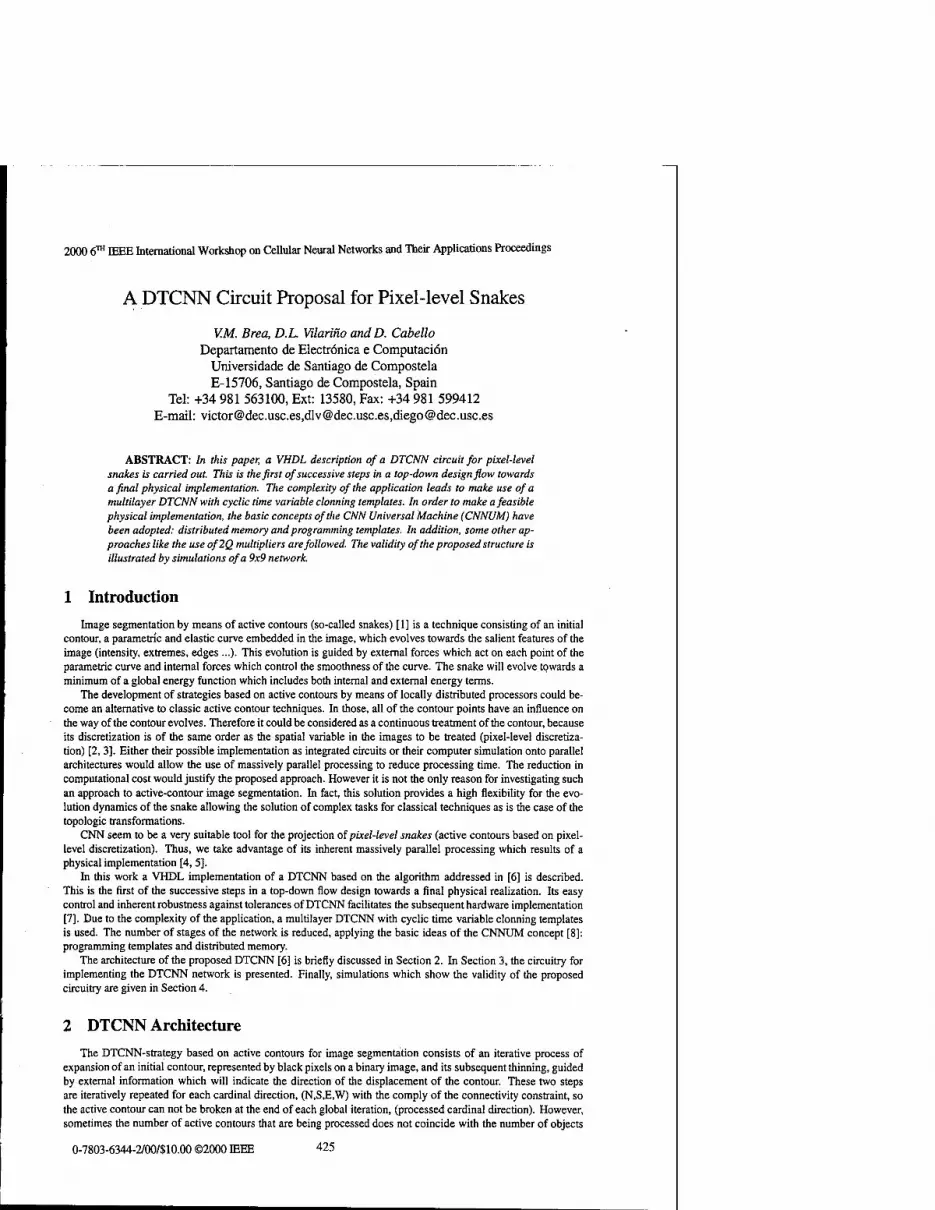
2000 6™ IEEE International Workshop on Cellular Neural Networks and Their Applications Proceedings

A DTCNN Circuit Proposal for Pixel-level Snakes

V.M. Brea, D.L. Vilarino andD. Cabello Departamento de Electrönica e Computation

Universidade de Santiago de Compostela E-15706, Santiago de Compostela, Spain

Tel: +34 981 563100, Ext: 13580, Fax: +34 981 599412 E-mail: victor@dec.usc.es,dlv@dec.usc.es,diego@dec.usc.es

ABSTRACT: In this paper, a VHDL description of a DTCNN circuit for pixel-level snakes is carried out. This is the first of successive steps in a top-down design flow towards a final physical implementation. The complexity of the application leads to make use of a multilayer DTCNN with cyclic time variable donning templates. In order to make a feasible physical implementation, the basic concepts of the CNN Universal Machine (CNNUM) have been adopted: distributed memory and programming templates. In addition, some other ap- proaches like the use of2Q multipliers are followed. The validity of the proposed structure is illustrated by simulations of a 9x9 network.

1 Introduction

Image segmentation by means of active contours (so-called snakes) [1] is a technique consisting of an initial contour, a parametric and elastic curve embedded in the image, which evolves towards the salient features of the image (intensity, extremes, edges ...)• This evolution is guided by external forces which act on each point of the parametric curve and internal forces which control the smoothness of the curve. The snake will evolve towards a minimum of a global energy function which includes both internal and external energy terms.

The development of strategies based on active contours by means of locally distributed processors could be- come an alternative to classic active contour techniques. In those, all of the contour points have an influence on the way of the contour evolves. Therefore it could be considered as a continuous treatment of the contour, because its discretization is of the same order as the spatial variable in the images to be treated (pixel-level discretiza- tion) [2, 3]. Either their possible implementation as integrated circuits or their computer simulation onto parallel architectures would allow the use of massively parallel processing to reduce processing time. The reduction in computational cost would justify the proposed approach. However it is not the only reason for investigating such an approach to active-contour image segmentation. In fact, this solution provides a high flexibility for the evo- lution dynamics of the snake allowing the solution of complex tasks for classical techniques as is the case of the topologic transformations.

CNN seem to be a very suitable tool for the projection of pixel-level snakes (active contours based on pixel- level discretization). Thus, we take advantage of its inherent massively parallel processing which results of a physical implementation [4,5].

In this work a VHDL implementation of a DTCNN based on the algorithm addressed in [6] is described. This is the first of the successive steps in a top-down flow design towards a final physical realization. Its easy control and inherent robustness against tolerances of DTCNN facilitates the subsequent hardware implementation [7]. Due to the complexity of the application, a multilayer DTCNN with cyclic time variable clonning templates is used. The number of stages of the network is reduced, applying the basic ideas of the CNNUM concept [8]: programming templates and distributed memory.

The architecture of the proposed DTCNN [6] is briefly discussed in Section 2. In Section 3, the circuitry for implementing the DTCNN network is presented. Finally, simulations which show the validity of the proposed circuitry are given in Section 4.

2 DTCNN Architecture

The DTCNN-strategy based on active contours for image segmentation consists of an iterative process of expansion of an initial contour, represented by black pixels on a binary image, and its subsequent thinning, guided by external information which will indicate the direction of the displacement of the contour. These two steps are iteratively repeated for each cardinal direction, (N,S,E,W) with the comply of the connectivity constraint, so the active contour can not be broken at the end of each global iteration, (processed cardinal direction). However, sometimes the number of active contours that are being processed does not coincide with the number of objects

0-7803-6344-2/00/S10.00 ©2000 IEEE 425

in the scene. In these cases, correct splitting and/or merging of the corresponding active contours [6] are needed in order to perform a correct topologic transformation.

In this approach, there is a pixel-level discretization, in which all of the contour points have influence on the way the contour evolves. Thus the concept of pixel-level snake is being applied to solve the problem of image segmentation [3].

The building blocks of the algorithm are shown in the block diagram of figure 1. The CE module performs the contour evolution, guided by external information, while CPD and CPE modules accomplish the topologic transformations. Figure 2 shows the architecture of the DTCNN network for a given processing direction.

The external energy, (previously calculated), is processed by the EP block of figure 2. Its input is a real value array, in which each real value is codified by an eight bit word. The EP output is a binary image (one bit word), whose white pixels indicate valid locations to move the contour. The output from EP indicates the direction of the gradient, which guides the active contour towards the minimum of external energy. Since the EP block processes eight bit words, its structure will be different from the rest of the blocks of figure 2, which process the active contour (black pixels on a binary image), so the minimum number of layers necessary for the application is two, one for the EP block, and other one for the rest of the blocks.

The operation of EXP processing steps of figure 2 consists of performing a duplication of the contour along the direction under consideration. This operation will be carried out if the location of these new activated pixels corresponds with white pixels of the EP output. Following, TH blocks carry out the thinning operation, deactivat- ing those active pixels that have been duplicated in the EXP(2) cycle. Nevertheless, the connectivity of the active contour must be restored in case of rupture, during the TH(3) and TH(4) cycles.

The result of the operation of the CPD module is the detection of possible collision points in the next global it- eration. The output from CPD module is an one-pixel wide wall between two active contours pieces that otherwise could collide. The CPE block performs the correct splitting and/or merging of the corresponding active contours when the continuity is guaranteed. The templates designed for a correct support of topologic transformations have been discussed in [6].

• Since each layer (block) is connected in series with other one, it is possible to replace the instant over space by replay over time. This is achieved by programming templates and the use of local logic memories (LLM), controlled by a global programming unit (GAPU) [8], which will be explained in the next Section. The aforemen- tioned programming templates are repeated after the processing along the four cardinal directions while a stable output is not reached.

External Information

J_

C^D T"

Contour Image

Figure 1: Diagram of the building blocks of the algorithm.

^ EXPO)

A

!—I—I—1 A

TH(1) CPE/1) Lä

!—I 1

r CP&3) A

CP&4) A

C?tX2) ^

Figure 2: DTCNN architecture, with its processing steps and interconnections.

426

3 Circuitry of the Cell

The network to be implemented is a multilayer DTCNN with cyclic time variable clonning templates [7, 9], with some of the funcionalities of the CNNUM [8]. The DTCNN network described in this work is characterized by the use of a clock signal, elk, which divides the operation of the cell in two steps [9]. Firstly, when elk is on, the internal state Xc is calculated. This is done from an offset term, common to all cells of the network, and from the outputs of layers that have been processed a few cycles before (eg. Vj,, means the output of the layer L). In the following step, with elk off, the present output Yc is obtained after a thresholding of Xc. This mode of operation is summarized in the equation 1

Yc(k) = sgn { X' = £ {A%Ytx + B"dYt2 + offset) (1)

where A and B represent the clonning linear templates used in our application, in which each cell is driven by nine cells, including the cell itself. So the degree of neighborhood, indicated by the subscript r, is one.

Figure 3 shows a schematic circuitry representing the DTCNN architecture of figure 2. The complete circuitry will be explained later. In figure 3 it can also be seen a transistor-level realization of equation 1. It is implemented by LLM(O) which consists of two dynamic memories, driven by complementary switches [9], This way, when elk is on, the internal state X" is set at the gate of the first inverter in LLM(O). Following, when elk is off, the present output Y" = outdO is obtained.

II -1

ttujfl OHJ1 Oul <M>1 CHU* OnjJ Otjt CM_>1 0M_*

_ _EPPn™tjajB_lock_

cuKSbltA

osl_ton | LLM(0) 'oul_™ ' •»•.«on j LLM(O) ' LLM(0) ' LtM(O) ' LLW(0) ' LLM(0) ' UM{0)< LLM(O)' LLM<0)' ILM(O) ' LLM(0) ' LLM(0} ' ! UM(4) ! LIM(6) LLM<2} UAi(4) LLM(fi) ' LLM(I) ' LLM(I)' LLM«)' ' LLM(2) ' "-"«> ' '

Figure 3: Schematic representation of the circuitry described in VHDL, and the time diagram labeled with the layers of the architecture, and their associated LLM events.

As mentioned before, EP block guides the evolution of the active contours towards the minimum of external energy. The simplest approach is a comparison between the grey level of a given cell and its neighbor along the direction under consideration. The EP block processes external energy images codified by eight bit words in complement two mode. The result is a binary image in which each pixel is codified by one bit word: the sign bit. White pixels on the EP output represent positive values that permit the active contour to be shifted along the direction under study. The EP block is completed with an OR gate driven by the outputs from CPD(3) (figure 2). This way, those black pixels in the CPD (ie. collision points) output are projected onto the EP output.

The circuitry associated with the rest of the layers of figure 2, (without taking into account the EP block), consists of a FIFO memory, implemented by a shift register, in which each register is made by a LLM, as it can be seen in figure 3. The output of a LLM is transferred to the next at the end of one complete cycle of elk. Therefore it is possible to store the outputs from layers that have been operated a few cycles before. In our application, we need four LLM to reduce the fifteen layers of figure 2 to only two. The chronogram represented in figure 3 shows how this can be done. We have labeled the current processing cycle and the LLM that are being used in

427

that cycle. Each LLM is associated with one layer of figure 2. LLM that must be used are set by the current cycle processing, according with the time diagram of figure 3. This association between LLM and layers depends on the cycle processing, so it changes over time.

Programming templates and local switches controlled by global signals from a global programming unit (GAPU) [8], are the additional elements which makes that a given cell becomes a general cell, in the sense that it works like several layers. In addition, a special memory, indicated as ESM in figure 3, is necessary. This memory is used to store the active contour at the end of each cycle, and while the uploading of the contour image is being done. Finally, OR gates, that can be thought as not programmable local logic units (LLU) [8] complete the structure of the cell.

Programming templates of our application are codified by five bit digital words, using the complement two mode. Nevertheless, since some of the templates matrices are extremely sparse, we have represented the zero coefficients with only one bit. As a consequence, the programming template words present an irregular size. This makes a ROM more suitable than a RAM implementation to store them. In this application a ROM, controlled by a 15-module synchronous binary counter (SBC) is used. SBC counts the number of processing cycles of elk (layers of the archictecture shown in figure 2) for each global iteration (processing direction).

Local switches that select the LLM outputs which drive the multipliers A and B sire controlled by signals sel_a and sel_b in figure 3. These are generated from two finite state machines controlled by SBC in GAPU, (figure 4): FSMA and FSMB for A and B templates.

The selection of the appropriate direction to be processed in the EP block is carried out by the synchronous binary counter SBCEP in figure 4.

Finally, the rest of switches are controlled by the OSCG module of the GAPU. Figure 5 shows the complete chronogram of the network. The activation of signals sel_in_esm_or_d6 and clk_esm makes possible that the initial contour will be fed to the chip. Following, start signal goes on, and the network processing begins. In order to select between the two layers of the network, signal sel_adder_or_ep is generated. Finally, the signal sel_exp2_thl is necessary to select which layer between EXP(2) or TH(1) is driven by the EP output.

Since the CPD module (figure 3) detects locations corresponding to possible collision points in the next global iteration, the direction of templates is changed at the beginning of CPD(l). Likewise the EP cycle will do the comparison between one pixel and its neighbor along the next processing direction.

The output of each cycle is calculated at the end of CPE(4) and transferred to ESM at the beginning of EP, so at this moment elk esm is activated.

T/

CONTROL SIGNALS

TO THE ARRAY CELL

Figure 4: Symbolic view of the global programming unit common to all cells.

3.1 Multipliers for the A and B templates

Saturated levels of the thresholding function that result from the equation 1, which gives the mode of operation of the DTCNN implemented, are zero and one. This means that a 2Q multiplier may be used. For doing this, 4Q templates have to be transformed into 2Q templates. The transformation followed is set by the equation 2

Au = 2Au §u = 2Bkl

offset = offset - £,., (Aki + BH)

(2)

where Au and Bki represent the coefficients of the original 4Q templates, and the symbol "denotes new 2Q multipliers.

This transformation allows the multipliers, represented in an schematic form in figure 3, to be implemented by a simple switch-multiplexor. If the signals from LLM are oh, the weigh coefficients, Wa and Wb are selected. If the signals from LLM are off, the output of the multipliers is zero.

428

, Processing along » given direction

■el.epffljj

■el_ep(l>f

EXP(l)lEXP(l)lEXP(2)lTH(l)lTH(2)lTH(3)lTH{4)lCPE(l)lCPE(2)lCPE(3)lCPE(4)lCPD<l)lCPD<2)lCPD<3), EP ' EXP(l)

Figure 5: Time-diagram of the control signals which drive the array cell from the GAPU.

4 Example of Application: A Topologic Transformation

We have described a 9x9 network in VHDL in order to show the validity of the proposed structure. We have assumed the default delta-time for the delay of the circuitry. This circuitry can be thought as an ideal representation of transistor-level devices that will be designed in a subsequent step of the top-down design flow. In this stage of design, we have shown a correct time relation between all events within the network and a correct operation of the templates designed for the application.

An example of image segmentation that requires a topologic transformation is shown on the left side of figure 6. Since there is only one object in the scene and two active contours, a correct split and merging of these will be realized at the end of the evolution. On the right side of the same figure we have represented the external energy within a 9x9 window, the same size of the network described in VHDL. The external energy has been obtained from the distance to the closest boundary points, and it is scaled from 0 to 255, (eight bit words), as it can be seen. The most meaningful frames from the contour evolution during the first four processing directions, in which a topologic transformation takes place, have been extracted. The order followed for the different processing directions is in the clock-wise sense, starting from the north and finishing by the west.

The first global iteration (north direction) works without the external energy processing. Nevertheless, before the processing starts, a reset elk cycle, which sets all outputs from the different LLM and EP off, is performed. As a consequence, EP output is a white image which shifts one pixel in both initial active contours of figure 6 along the north direction, at the end of the CPE(4). This frame result is shown in figure 6. Following, the contours do not change along the east processing direction.

As it can also be seen in figure 6, during the south processing direction, the top active contour is one-pixel shifted to the south, at the end of the TH(4) cycle. As a result, there is an one-pixel wide wall between the two contours, so a topologic transformation is realized by the CPE module. In figure 6, the four stages of the CPE module are shown. Firstly, the one pixel wide wall is actived on CPE(l). These pixels are deactivated on CPE(2). Finally, the continuity of the contours is restored during the CPE(3) and CPE(4) stages, and a topologic transformation have been realized by the network circuitry. This result is transferred to the next global iteration, west processing directiqn, in which there are not changes on the active contours.

5 Conclusions

In this paper a VHDL description of a 9x9 DTCNN network which implements an operation of pixel level snake has been discussed. The complexity of the application leads to the use of a multilayer DTCNN with cyclic time variable clonning templates. The number of the initial fifteen stages is reduced to only two, by means of the use of the basic concepts of the CNNUM: programming templates and distributed memory.

The VHDL description shown in this paper, is the first of successive steps in a top-down design towards a final physical implementation. In this stage of design, we have shown a correct time relation between all events within the network and a correct operation of the templates designed for the application.

The templates used for the application are 2Q templates, which means that a zero-one representation of the sat- urated levels of the thresholding function in the DTCNN equation. This allows to use simple switch-multiplexors

429

Topologic Trans formal ion in a 32x32 Image

I

1 !

sr ■ ■ II ■ :■ ■ _:■ liiiiil Atfive C

If.

Eiittiul Entriy Imige

CPE(2) CFEP)

Figure 6: Example of an image segmentation that requires a topologic transformation, in which the most mean- ingful frames of the contour evolution within a 9x9 window have been extracted.

for the A and B templates implementation. The devices which may be used for the analog part in a successive step of the flow-design, such as current-

steering D/A converters for the A and B templates, and a simple node (Kirchhoff Current Law) to add the currents from the multipliers, can be viewed as ideal devices. The precision which presents these devices is set by the number of bits used to codify the analog values. The default VHDL delta-time is assumed for the delay of the devices implemented.

The validity of the proposed structure is illustrated by a VHDL simulation of a topologic transformation along the vertical direction in a 9x9 network.

Acknowledgment The assistance of Alejandro Pineiro (Alex), a Ph. D. Student in Departamento de Electrönica e Computaciön

of Universidade de Santiago de Compostela is gratefully acknowledged.

References

[1] M. Kass, A. Witkin, and D. Terzopoulos "Snakes: Active Contours Models" International Journal Computer Vision, (1):321-331,1988.

[2] D.L. Vilarino, V.M. Brea, D. Cabello and J.M. Pardo "Discrete-Time CNN for Image-Segmentation by Active Contours" Pattern Recognition Letters, 19(8), pp. 721-734,1998.

[3] D.L. Vilarino, D. Cabello, J.M. Pardo and V.M. Brea "Pixel-Level Snakes" Submitted to International Con- ference on Pattern Recognition, Barcelona, September 2000.

[4] Gustavo Linan, Rafael Domfnguez-Castro, Servando Espejo and Angel Rodriguez-Vazquez "Design of a Large-Complexity Analog I/O CNNUC" Design Automation Day on Cellular Visual Microprocessor, EC- CTD'99, pp. 42-57, 1999.

[5] Ari Paasio, Asko Kananen and Veiko Porra "A 176x144 Processor Binary I/O CNN-UM Chip Design" Design Automation Day on Cellular Visual Microprocessor, ECCTD'99, pp. 82-86,1999.

[6] D.L Vilarino, D. Cabello, T. Kozek, J.M. Pardo and V.M. Brea "Topologic Transformations in Active Con- tours: A DTCNN-Based Approach" In Proceedings of European Conference on Circuit Theory and Design, ECCTD'99, pp. 1351-1354,1999.

[7] H. Harrer, J.A. Nossek and R. Stelzl "An Analog Implementation of Discrete-Time Cellular Neural Network- s'', IEEE Transactions on Neural Networks, vol 3, n 3, pp. 466-476,1992.

[8] T. Roska and L.O. Chua "The CNN Universal Machine: An Analogic Array Computer", IEEE Transactions on Circuits and Systems, vol. 40, n 3, pp. 163-173,1993.

[9] V.M. Brea, D.L. Vilarino and D. Cabello "A Compact and Robust Circuit Proposal for Reconfigurable DTC- NN" In Proceedings of European Conference on Circuit Theory and Design, ECCTD'99, pp. 940-943, 1999.

430

2000 6™ IEEE International Workshop on Cellular Neural Networks and Their Applications Proceedings

IC Design of 8x8 Digital CNN with Optoelectronic Interface

S. Jankowski, A. Wielgus, W. A. Pleskacz, R. Buczyfiski, M. Wiiniewski

* Institute of Electronic Systems, Warsaw University of Technology, ul. Nowowiejska 15/19,00-665 Warsaw, Poland

b Institute of Microelectronics and Optoelectronics, Warsaw University of Technology, ul. Koszykowa 75,00-662 Warsaw, Poland

" Lab for Photonics, Faculty of Applied Sciences, Vrije Universiteit Brüssel, Pleinlaan 2, B-1050 Brussels, Belgium

ABSTRACT: The paper presents a new optoelectronic CNN system which consists of two integrated circuits connected through the flip-chip bonding: a) the photonic GaAs matrix of receivers and emitter; b) the CMOS chip of digital CNN cells with programmable 5-bit weights and threshold currents. This solution is easier to design and is more reliable than analogue circuits. The main advantages of our system include parallel input/output of considered image and high precision of programmable weights. Although the processing speed of the digital CNN is considerably lower than that of analogue implementations, it is fast enough for efficient image processing by complex CNN programs.

1. Introduction

Massively parallel processing systems, as CNN, are facing an input/output bottleneck nowadays. The most promising method to overcome this problem seems to be a parallel optical input/output interface, where every processor (cell) possesses its own optical input and output [1, 2]. Such an optoelectronic system consists of two main parts. The first part is an optoelectronic chip made of GaAs that provides optical emitters and receivers [1]. The second part is silicon CMOS circuitry where all the data processing is performed. In this paper we present a new design of an array of 8x8 simple digital processors that are able to perform operations on binary images using 5-bit programmable weights.

2. General Concept of the System

The functional scheme of our photonic processor with optical interconnects is presented in Fig. 1. The input discrete intensity distribution impinges on the detector array of the optoelectronic chip. The result recorded by the detectors of the optoelectronic chip is fed into the VLSI circuit through solder bumps. The electric signals that enter the cells of the CMOS chip are processed digitally according to the programmed algorithm.

When the CNN program is finished the output data matrix is sent in parallel from CMOS chip to emitters on the optoelectronic chip via solder bombs and then the signals are sent out by means of an optical link.

Optical parallel data Input/Output ►

GaAs Optoelectronic chip Flip-chip bonding interconnections

Silicon CMOS chip

Flip-chip bonding \ y^ Photoaics interconnections

Figure 1: The general scheme of a photonic digital CNN: Ml - lens, Gl-diffractive optical fan-out element to implement local programmable optical interconnects, optoelectronic chip -a matrix of receivers and emitters, silicon CMOS chip - CNN circuitry with electrically programmable interconnects.

0-7803-6344-2/00/$10.00 ©2000 IEEE 431

This architecture enables to perform two ways of CNN processing realisation. In the first case CNN templates are realised electronically. The digitally calculated final results are fed back into the optoelectronic chip and activate the emitters. In the second case CNN templates are realised optically via a programmable diffractivc grating Gl corresponding to well-defined CNN operators.

3. Architecture and Processing of Digital CNN

As stated in the previous section, the photonic chip provides parallel data input to and output from the electronic chip through the flip-chip bonding. The electronic chip performs digital processing of the supplied data and sends the results back to the photonic chip.

i IT*

1 ÜU

n mr i-

□ n

I-'In.

* i mi i—

+ ° a - -4IL IB-

" 1 DC

-.-in

IT

-

t III

-J

IL_T D 0

,11 I D D

11 r >--

D D D C

H--1 1 fll IT*-- D □

III 1 .

ILJ, H 0 D

i it 0 D

--! it

^ I — H 1-

D C

►--in

i)

ill rh

□ D D D

1 IL

h r a D

.Jl UILH

,1 -HI-

D r.

h 'I p*nm_<mt<t.O>

«d* <40> 1 «nr<1:0>

1 ' 'rBxrt

- RAM Control

Automaton Counter mod19

||

clk1

9

rese

t

.mod

e

[

Figure 2: Architecture of the CNN integrated circuit.

The architecture of the CNN integrated circuit is shown in Fig. 2. Each cell in the network is connected with the eight neighbouring cells and with one cell in the photonic chip. It obtains the input signal «*, from the photonic cell and the data, consisting of the input signals uMJfi and the output signals ymj^ , from all neighbouring cells. This data is processed together with the stored output signal y^. The result is stored in the cell and sent back to the connected photonic cell. Data processing is performed in accordance to the state and output equations of DT CNN:

l l l l xij — 2-i 2-1 ™iii+kj+iyi+kj+i ■*■ 2-i2-i "iß+tj+iun-tj+i ■*■'!/

1 x, > 0 (l)

y,i l-l x, <0

where x-,j is the state of the cell (i,j), «,y and yy are the input and output signals while A, B and / denote the feedback coefficient, the control coefficient and the threshold, respectively. We assume that all cells use the

432

same set of coefficients which enables to exclude the RAM module from a cell and share it among all cells in the 8x8 matrix. Otherwise, the RAM module, storing the coefficients, should be incorporated into each cell in order to assure more flexibility in image processing. The unit, consisting of the control circuit, the addressing circuit and the RAM circuit, is responsible for programming and controlling the performance of the CNN. It communicates with the computer system which sequentially stores a set of 19 coefficients in the memory during programming phase and then initialises neural processing.

The following assumptions on data representation have been made: • feedback coefficients Aijkl, control coefficients BiiU and the threshold / are represented by 5-bit numbers in

2's complement code, • input and output signals, u,y and>s, take only two values: '1' and '-1* which are 1-bit coded as '1' and '0',

respectively.

4. Digital CNN Cell

Circuit implementation of a single CNN cell is illustrated in Fig. 3. Single neural operation includes state calculation and output calculation. The state of a cell is calculated as the weighted sum of the output and input signals from the given cell and its eight neighbours according to the equation (1). In each clock cycle a new address is generated which selects a pair of signals: the 1-bit input signal from the multiplexer muxjtut and its corresponding 5-bit coefficient from the memory param. These two signals are multiplied and the result is added to the state register.

a) paramjn

start_mode

reset Control and Programming Unit

MuNpliff [Brando

Jio TL«B t«

DCNN Cell

ftegittor J DFF

b)

Figure 3: Digital implementation of the CNN Cell: a) block diagram; b) multiplier circuit.

433

The choice of the coding style, described in the previous section, enables to simplify significantly these two operations. The coefficients and the state of a cell are represented in 2's complement code. It allows direct addition of positive and negative numbers. As the muxjout signal takes two values meaning "1" or "-1", multiplication reduces to the following operation:

f param mux _out = l param x mux _out = \

[param + l mux_out = 0 (2)

The circuit implementation of the multiplier is presented in Fig. 3b. The most significant bit of the multiplier output signal param_sig has to be multiplicated five times, as shown in Fig. 3a. This operation preserves the sign of the signal value. State calculation completes after 19 clock cycles. The result is stored in the state register. The output of a cell is obtained as a complement of the most significant bit, e.g. the sign bit of the cell state. This value will be held in the output DFF until the completion of the next neural operation.

5. Control and Programming Unit

As shown in Fig. 4, the Control and Programming Unit consists of three modules: • RAM which stores 19 numbers of 5-bit size parameters, • Counter mod 19 which generates addresses, • Control Automaton that controls all modules.

Control and Programming Unit

y start_mode -

reset Control Automaton sm

elk c*

y Counter „, mod 19

elk

/

addr addr

\ : > t

¥ RAM addr param_in duur

param_oul S, /

8/

elk smr addr param

reset DCNN Cell

^T Uu

Figure 4: Block diagram of the Control and Programming Unit.

Table 1 defines the states transitions and the output signal smr of the automaton that controls all other modules.

start_mode addr

00 01 10 11 00 10011

01 10011

10 10011

11 10011

state

wait sO sO 00

si 01

si 10

s2 11

- - - -

load si sO si si sO _ sO sO _ 00 01 10 00 - 00 00 -

compute s2 s2 s2 s2 s2 sO sO sO sO next_state

smr /; ;/ 11 11 00 00 00 00

Table 1: Description of the Control Automaton.

434

The control of the system is provided by 2-bit startjnode input signal. Depending on the value of this signal, the Mealy control automaton is in one of the three states. The initial state is the wait state when the control automaton waits for the signal start_mode="01" starting the programming phase. Automaton changes its state to load and sets up the new address as a current counter state. When startjnode signal becomes "10", the input data, coming from the computer, is stored in RAM at proper address. Simultaneously the counter state is incremented. The sequential repeat of the values "01" and "10" causes storing of all 19 parameters in the memory. Setting up value "11" on startjnode input initialises the phase of computing the states of all cells.

6. Results

Our circuit was designed in the standard cells style. The VHDL model was synthesized and optimized using commercial CAD tools. The layouts of the 4x4 CNN circuit and the main building blocks, the CNN Cell and the Control and Programming Unit, have been obtained. The parameters of these layouts in AMS 0.35 |im CMOS technology are summarized in Table 2.

Design unit Area [um2]

CNN cell 26391

Control and Programming Unit 60619

8x8 CNN IC 1783515

Table 2: Layout parameters of the 8x8 CNN chip in AMS 0.35 CMOS technology.

Logic simulations of the synthesised circuit were performed in order to verify its functionality and to estimate the most important timing parameters. The results are presented in Table 3. Given clock frequency is the maximal value obtained during logic simulation of the synthesised circuit where no parasitic elements were considered. There is a need to accept that the real operation frequency of the CNN circuit is supposed to be lower.

Parameter Value

Maximal clock frequency [MHz] 330

Time of one clock cycle [ns] 3

Time of programming phase [ns] 114

Time of computing phase [ns] 60

Time interval between programming and computing phases [ns] 6

Table 3: Timing parameters of the 8x8 CNN chip in AMS 0.35 CMOS technology.

7. Conclusions

In this paper the design of fully digital programmable CNN with optoelectronic interface is presented. This system consists of two integrated circuits connected through the flip-chip bonding: the photonic GaAs matrix of receivers and emitters and the CMOS chip of digital CNN cells. Our solution is easier to design and is more reliable than analogue circuits, e.g. [8, 9]. The advantages of our system are the following: • parallel input/output of considered image, • programmable weights of high precision. Although the processing speed of the digital CNN is considerably lower than that of analogue implementations, it is fast enough for efficient image processing by complex CNN programs.

435

8. Acknowledgements

The authors would like to thank Prof. Wieslaw Kuzmicz, Dr. Zbigniew Jaworski, Dr. Elzbieta Piwowarska, and Mr. Marcin Sadowski from Warsaw University of Technology, Prof. Alexis de Vos from University of Ghent, Mr. Arto Rantala from VTT and Prof. Hugo Thienpont, Prof. Irina Veretennicoff from Vrije Universiteit Brussels for their help and very valuable feedback.

9. References

[1] R. Buczyhski, H. Thienpont, S. Jankowski, T. Szoplik, I. Veretennicoff: "Programmable CNN based on optical thyristors for early image processing," Proc. of the Fifth IEEE Int. Workshop on Cellular Neural Networks and their Applications CNN A 98, London, pp. 259-264, 1998.

[2] S. Jankowski, R. Buczyhski, A. Wielgus, W. Pleskacz, T. Szoplik, I. Veretennicoff and H. Thienpont: "Digital CNN with Optical and Electronic Processing," Proc. European Conference on Circuit Theory and Design ECCTD'99, Stresa - Italy, pp. 1183-1186, 1999.

[3] R. Buczyiiski, V. Baukens, T. Szoplik, A. Goulet, N. Debaes, A. Kirk, P. Heremans, R. Vounckx, I. Veretennicoff, H. Thienpont: "Fast optical thresholding with an array of optoelectronic transceiver elements," IEEE Phot. Techn. Lett., vol. 11, pp. 367-369, 1999.

[4] T. Roska and L. O. Chua: "The CNN universal machine: an analogic array computer," IEEE Trans. Circuits Syst., vol.40, pp. 163-173,1993.

[5] A. Zarandy, F. Werblin, T. Roska., L. Chua: "Spatial logic algorithms using basic morphological analogic CNN operators," Int. J. Circuit Theory andAppl., vol. 24, pp. 283-300, 1996.

[6] T. Ikenaga and T. Ogura: "A DTCNN universal machine based on highly parallel 2-D cellular automata CAM," IEEE Trans. Circuits Syst I., vol. 45, pp. 538-546, 1998.

[7] A. G. Kirk, H. Thienpont, A. Goulet, P. Heremans, G Borghs, R. Vounckx, M. Kuijk, I. Veretennicoff: "Parallel optoelectronic data transcription with fan-out between planes of PnpN optical thyristors," IEEE Phot. Techn. Lett., vol. 8, pp. 464-466, 1996.

[8] A. Rodriguez-Vazquez, E. Roca, M. Delgado-Restituto, S. Espejo and R. Dominguez-Castro: "MOST- Based Design and Scaling of Synaptic Interconnections in VLSI Analog Array Processing CNN Chips," Design Automation Day, Proc. European Conference on Circuit Theory and Design ECCTD'99, Stresa - Italy, pp. 15-41, 1999.

[9] A. Paasio, A. Kananen and V. Porra: "A 176 x 144 processor binary I/O CNN-UM chip design," Design Automation Day, Proc. European Conference on Circuit Theory and Design ECCTD'99, Stresa - Italy, pp. 82-86,1999.

436

2000 6™ IEEE International Workshop on Cellular Neural Networks and Their Applications Proceedings

Cellular Nonlinear Network Implementation for Nonlinear B-Template

Ari Paasio, Kari Halonen

Electronic Circuit Design Laboratory, Helsinki University of Technology P.O.Box 3000, FIN-02015 HUT, FINLAND

phone: +358-9-451 5013 fax: +358-9-451 2269 e-mail: apa@ecdl.hut.fi

ABSTRACT: In this paper a design for a nonlinear B-template is overviewed. The design is targeted for a 0.25 micron digital CMOS process. The transistor level schematics are given together with simulation results. Also the layout is reported.

1. Introduction

Several applications have been developed for CNN that require a dedicated hardware in order to achieve a real time algorithm execution. Many of these algorithms include nonlinear templates which have not been realized yet in the existing hardware implementations. In this paper a circuit realization will be given that is suited for implementing a particular nonlinear B-template with reasonable silicon area. The suggested approach is suited for nonlinearities which consist of taking the absolute value of the inputs or the absolute value of the differences between the inputs. The latter case, namely the difference controlled one, is overviewed more closely.

2. Overview of the processing task

2.1 Template task description

In [2] a video segmentation algorithm was presented that introduced several CNN templates. One of the most challenging templates, from the implementation point of view, was the nonlinear template that is used for gradient estimation. The template is given as

[0 0 ol \b b b] 0 10 B = b 0 b 0 0 0 b b b

I = thres (i)

where the element b is graphically shown in Fig.l.

Figure 1: Nonlinear B-template element.

The meaning of the element b is that it takes the difference of the cell input and the input of the corresponding neighbor cell, and additionally calculates the absolute value of the difference. Additionally, in the above template there are two nonzero entries, namely the unity self-feedback and the bias template valued thres. The operation of the whole template is to evaluate contributions given by the nonlinear B-template and to compare that contribution to the value thres. Then depending on the result of the comparison the cell output will evolve to a stable bipolar value, due to the positive feedback. Now, although this template is given with the self-feedback entry, it is only used to drive the output either black or white. Because this is the only purpose of the self-feedback in this template it can be omitted in the realization if the described functionality can be preserved. This approach is actually taken in the structure introduced below.

0-7803-6344-2/00/$10.00 ©2000 IEEE 437

2.2 Overall processing arrangement

If there are no off-center non-zero elements in the A-tempIate, then there are no propagation effects and the processing task can rather easily be performed by a reduced size network. This is suggested e.g. in [3], where the dimension of the CNN network in a vertical direction was reduced to one. This approach is taken here also, mainly because the input to the cells can be conveniently handled. In the arrangement where one image row is evaluated at a time, information is required from three image rows to guarantee correct border values. The inputs are required from the row below and from the row above in addition to the actual row being evaluated. This means that each processing element needs to get pixel information from three different rows and then these values should be distributed accordingly. This is shown in Fig.2.

ill III

^ LL

CELL

Figure S: Method for providing inputs to the processing cells.

In this arrangement there are three input lines to the cell and it has to be determined which line cor- responds to which row. The selection of the content of these three lines can be done in two instances. Namely, at each time a new row is introduced to the processor grid the information concerning the two rows still required for evaluation can be changed to be input through a different input wire corresponding to their relative location. In this situation the selection is made in the circuitry providing the input to the nonlinear cells and the information changes in each input line preceding the row evaluation time. Another approach, where the switching is reduced in the circuitry providing the input is to determine the relative locations of the contents of the input lines inside the cell. In this arrangement, the input information is written to an input line only once. This latter approach is illustrated in Fig.3 and adopted in the design in this paper.

g g y- t* m * s s 3 o o

Figure 3: Alternative method for providing inputs to the processing cells.

3. Internal pixel value coding

In the design it is preferable that the input values of the cells are coded in such a manner that the hardware realization of the nonlinear cell is simple. This requirement can be fulfilled using unipolar current signals as input values. In our design the white input pixel is represented by a 5/iA input current and the black input pixel is represented by a current 15/iA. The grey levels are between these two limits. This coding means that the unity current is 5/iA. By using the above coding, the end result of the absolute value calculation still remains the same as when using bidirectional input currents with unity value 5/jA, e.g. | - 5/iA -5/xA| = 10/iA and |5/JA -15/IA| = 10/iA, where a white pixel is evaluated together with a black neighbor pixel.

438

4. Cell circuitry

As stated in the above sections, the tasks performed by the cell circuit can be divided into three separate parts. These are, first selecting the relative locations of the input rows. Secondly, there is the calculation of the absolute values of the differences between the cell input and its corresponding neighbors. The third task is to compare the sum of the absolute values to a predetermined threshold value and to output the result of the comparison. The different parts of the cell will be presented separately in the following.

4.1 Row location selection

In the design three control signals are used to determine the row configuration. These signals are denoted by Cl, C2 and C3 and the corresponding switch configuration is shown in Fig.4.

s a a 3 3 1

^5 .Cl Cl

-5 -51 ^ca

^ca -C2 -Cl

—»- now+i

Figure 4-' Row selection configuration inside the cell

Because switching at input was to be omitted, the input signals are first copied and only after that the switching takes place. Moreover, because the cell input information is needed in the cell column and in the neighboring columns also, the current has to be copied into three different locations. The overall circuitry corresponding for the distribution of one input current is shown in Fig.5.

tVDD

INPUT CURRENT

Figure 5: Input information distribution circuit for one input line.

In the above figure the control signals are denoted by CX, CY and CZ and because in the cell there are three structures like that in Fig.5 the actual signals Cl, C2 and C3 are assigned to these nodes accordingly. In the described circuit the current is copied using simple current mirror with three outputs.

4.2 Absolute value calculation

The calculation of the absolute value can be effectively implemented by using a structure suggested in [4]. The circuit for evaluating one absolute value of the difference of inputs is shown in Fig.6. The input currents INI and IN2 are from the corresponding current sources shown in Fig.5 and the input current IN2 is inverted in a current mirror formed by M7 and M8. The difference of these input

439

vss

Figure 6: Absolute value evaluation circuit.

currents entering the absolute value evaluation circuit is denoted by UN in Fig.6. For a more detailed description of the functionality of the circuit the. reader is referred to [4]. The output of the block is current IOUT. Because also the output is current the summing of absolute value circuit outputs is performed by simply wiring.

4.3 Threshold comparison

After the eight absolute values corresponding the eight template entries in the nonlinear B-template have been evaluated the output currents are summed by wiring the output nodes of these blocks to an n-type current mirror. The sum is also scaled down by 10 to reduce the maximum possible current entering the comparator. This scheme is shown in Fig.7.

isVDD

i>H>o^-°

vss

Figure 7: Threshold comparison scheme.

In the above figure the sum of the absolute values is represented by a current ISUM-ABS, originating from eight absolute value evaluation blocks. The scaled version of this current is compared to a threshold current IJTHRES by an inverter acting as a current comparator. The current ISTHRES is provided to the cell through a p-type current mirror. The output of the inverter chain is the output of the cell, denoted by CELL-OUT in Fig.7. The output is HIGH if the threshold is greater than the contribution of the B-template and vice versa.

440

5. Simulation results

In this section an HSPICE simulation result is given for a 3x1 network. The MOS parameters in the simulations are for the 0.25 micron process with level 50. The setup for the simulation is as follows. The contents of the input lines do not change, only the control signals £71, £72 and £73 and then the sum of the absolute value blocks are monitored in every cell. Moreover, the outputs of the cells are shown. The contents of the input lines are shown in Fig.8 where also the values of the border cells for zero flux condition are shown. The magnitudes are in micro amperes.

RDER I I BORDER

0| |0 BHEBH

Figure 8: Input configuration.

In the following simulation the configuration changes to that shown in Fig.8 at time 20ns and the sums of the absolute evaluation blocks are shown. The ideal output values should be 26, 31 and 34pA for the cells from left to right, respectively. In Fig.9 the there are the currents from the three absolute evaluation blocks inside the cell. The upmost chart is for the left column, the middle one for the middle column and the bottom one for the right column, respectively.

i : I

I '"■-''''

~s«.

i; t f ± t -:

_B~

I-?- d

\r i .-ff™. ~ -

Figure 9: Absolute value current sums.

According to simulations, the output currents are 25.9, 30.9 and 34.0pA at 100ns, therefore yielding correct behavior. The threshold value was set to 2.7/JA, and therefore the output of the leftmost cell should be HIGH and the outputs of the two other cells should be LOW. This situation is illustrated in Fig.10 where the outputs of the cells are shown.

6. Layout realization

The layout of the cell has been designed using a 0.25 micron digital CMOS process design rules. In this process there are six metal layers for routing. The layout of one cell with all the local and global interconnections is shown in Fig.ll. The dimensions of the cell are 171.9x13.15pm2. The switches are on the left, the absolute value evaluation blocks are in the middle and the comparator structure with inverter chain as an output buffer is on the right hand side of the layout.

441

m

i ■ ;

I

~r™

Figure 10: Cell outputs.

Conclusions

A design for a nonlinear B-template has been overviewed. The transistor level schematics have been given together with simulation results that show correct operation of the approach. The layout of the structure has been drawn and sent to process.

Figure 11: Cell layout.

Acknowledgments

This work is supported by the Academy of Finland (#1366361/99).

References

[1] L.O.Chua and L.Yang, 'Cellular Neural Networks: Theory', IEEE Transactions on Circuits and Systems, Vol. 35, pp.1257-1272, 1988

[2] A.Stoffels, T.Roska, L.O.Chua, 'Object-Oriented Image Analysis for Very-Low-Bitrate Video-Coding Systems Using the CNN Universal Machine', International Journal of Circuit Theory and Applica- tions, Vol.25, pp.235-258, 1997.

[3] K.Slot, J.Kowalski, J.Pacholik, P.Debiec, 'Cellular neural network based VLSI architecture for image processing', Proc. Fourth IEEE Int. Workshop on Cellular Neural Networks and their Applications, CNNA-96, Seville, Spain, pp.249-254, 1996.

[4] I.Baturone, S.Sanchez-Solano, A.Barriga, J.L.Huertas, 'Implementation of CMOS Fuzzy Controllers as Mixed-Signal Integrated Circuits', IEEE Transactions on Fuzzy Systems, Vol. 5, pp.1-19, 1997.

442

2000 6™ IEEE International Workshop on Cellular Neural Networks and Their Applications Proceedings

A CELLULAR NEURAL NETWORK FOR PEAK FINDING IN HIGH-ENERGY PHYSICS

C.Baldanza, F.Bisi, M.Bruschi, l.D'Antone. S.Meneghini, M.Rizzi, M.ZuJfa

Istituto Nazionale di Fisica Nucleare Viale Berti Pichat 6/2,40127 Bologna, Italy

Email: dantone@bo.infh.it Tel :+39 051 2095275 Fax :+39 0512095286

ABSTRACT: This report describes the hardware implementation of a two-dimensional Cellular Neural Network (CNN) performing an on-line clustering algorithm. After a general introduction to the Cellular Neural Networks, we consider a two-dimensional CNN that performs a cluster peak finding algorithm in a matrix of cells mapping a sub-region of a calorimeter, a detector largely used in high energy physics. The peaks of the energy clusters are found in one collision time of the particle bunches (96ns). Some quantitative parameters are given to optimize the architecture of the CNN implemented in a commercial Field Programmable Gate Array (FPGA).

1. Introduction

Experiments in high-energy physics are based on detectors, devices that allow recording of signals originating from particles that have been generated in collisions, (bunch crossing), and which pass at relativistic speed in some medium. Modern detectors in a large experiment consist of tens of different subdetectors with different characteristics, each of them with many thousands of individual channels. Signals usually are electric charges; they are stored locally until a subset of the collision, i.e. the triggered event, has been selected for further inspection. The signals are then digitized, on-line analyzed and finally recorded on more permanent storage for analysis in high-level computers. The original objects, after some data preprocessing and aggregation, can be visualized as images. Detectors may be quite different in their characteristics. The signals analyzed in this paper come from a calorimeter, i.e. a detector composed by many small stationary cells in three dimensions able to absorb particles and record the energy deposited. The calorimeter cells are usually arranged in regular grids perpendicular to the main impact direction of tracks; windows to be analyzed are typically several tens of cells, and typically, cluster centers have to found by maximum search or center-of-gravity computation. The present paper examines the FPGA realization of a two-dimensional CNN (2D CNN) that has been developed to elaborate data coming from an electromagnetic (e.m.) calorimeter. A field programmable gate array (FPGA) is an array of logic cells programmable by the user. The case discussed here below is the search of peak of interesting clusters in sub-regions of the detector. The proposed two-dimensional CNN, with suitable templates, performs the algorithm within each bunch crossing time (96ns).

2. Cellular Neural Networks

Cellular Neural Network (CNN) is an analog parallel computing paradigm defined in space, and characterized by locality of connections between processing elements (cells, or neurons). Such systems are best suited for problems defined in space-time, e.g. image processing tasks, partial differential equations systems, and so on, in which the information necessary to the evolution of the system from a certain point is contained within a finite distance of the same point. From a hardware point of view, the local interConnectivity of the array lends itself to practical VLSI implementations. Consider an M x N Cellular Neural Network, having M x N cells arranged in M rows and N columns. The basic unit of a CNN is called cell. Any cell on the ith row and jth column, C(ij), is connected only to its neighbor cells, i.e. adjacent cells interact directly with each other. This neighborhood is denoted as N(i,j). Cells not in the immediate neighborhood have indirect effect because of the propagation effects of the dynamics of the network. Each cell has a state x, a constant external input «, and output y. The first order nonlinear differential equation defining the dynamics of a cellular neural network cell can be written as follows:

0-7803-6344-2/00/S10.00 ©2000 IEEE 443

dt ■-xij(t)+ YJA(i_k)ü_l)(t)ytl+ Xä

<M>G-OW«H+' teN,<i.j) HeN,(i,j)

yi;(t) = Ux,J(t)+l\-\xij(t)-l\ (1)

where ytj represents the output equation, i.e. the activation function for the cell, and A(,.klu.n and B(i.tm are the space invariant programming templates for all cells C(k,l) in the neighborhood N(ij) of cell C(iJ). In a bidimensional grid with the interaction limited to the nearest neighborhood the templates contains, at most, 19 real numbers:

A);l

A;,

B =

B

B,. K. ... Sl:0 Sl;l

B„, (2)

The matrices are also known as cloning templates. A constant bias / and the cloning templates determine the transient behavior of the cellular nonlinear network. These 19 numbers control the whole CNN whatever its size is, i.e. the set of weights is size independent. This is the main difference between the CNNs and the formal neural networks. A acts on the output of neighboring cells and is referred to as the feedback operator. B in turn affects the input control and is referred to as the control operator. Specific entry values of matrices A and B are application dependent. The discrete time version of the CNN is described by the following equations:

xij(n + l)= JJA,jMytl(n)+ X %,«»+/<,

y,](n)=f[x,1(r,)] (3)

where the activation function/of the cell is the sign function or the usual PWL function as in Eq.l. The discrete time version is characterized by constant speed of information diffusion over the network, whereas in continuous time CNNs it cannot be explicitily controlled.

3. Clustering with ID and 2D CNNs

The calorimeters provide several particle selection types (trigger); one of the major goals is to identify electrons in order to start the next level trigger algorithm. The main process is the identification of a large energy deposit in a small region of the e.m. calorimeter. The described trigger algorithm performs basically a two-step computation: a search for the cell with the maximum energy, followed by the cluster processing around the maximum. The peak finding step permits concentrating the computing work in the interesting calorimeter cells. To perform the peak finding algorithm, we propose a two-dimensional CNN with the grid dimension mapping exactly the analysed sub-region of the calorimeter. We define a CNN cell with a value equal to the energy of the corresponding calorimeter cell. The energy values related to each calorimeter cell are usually digitized in about 12 bits and, after that, they are compressed in 8 bits to reduce the cabling and to increase the data transfer rate. With a suitable templates, the CNN evolves in one bunch crossing to a configuration in which only the peaks of the clusters are fired. This process can be considered as a two-dimensional filtering. The architecture that we will describe is effectively used in an actual experiment [4] [5]. To clarify the behaviour of the implemented two-dimensional cellular neural network we consider, at first, a simple binary one-dimensional CNN performing a clustering algorithm. Suppose we are using a CNN with 1 neighbour on eacli side and with the following templates:

A = [() 1 oj B = [-l 1 Oj / = -l (4)

Starting from some random configurations and using the Euler integration method with dt=0.1 and with the PWL output non linearity having the -I. +1 limits, the CNN output always reaches a stable state in a short time. At the

444

a) b)

fig.l. Cluster identification with a two-dimensional binary CNN with templates (6). Starting from the configuration in fig. la, the CNN evolves as shown in fig. lb.

steady state all the input clusters are grouped in one ouput cell, i.e. the CNN performs a clustering algorithm. For each cluster, the cell selected is the one located farthest on the left. We can extend the behaviour exhibited by the described one-dimensional CNN to a two-dimensional case with the following templates:

0 0 0"

0 1 0 , B =

0 0 0

0 0 0"

-1 1 0

0 -1 0

/=-! (5)

This 2D CNN exhibits a behaviour similar to described ID CNN, and can be used to perform the identification of the clusters. In fig.la is shown an initial random configuration in which five clusters can be identified. A bidimensional binary CNN with the templates (5), starting from the configuration in fig.la evolves, in a few time units, as shown in the fig. lb in which the extreme south-west pixel for each cluster is fired. If the cluster contains more points to the south-west extremity, i.e. cluster B in fig.la, it might be identified by more than a point (B' in fig.lb). This effect disappears, as we see afterwards, in grayscale CNN when states with more bits are considered.

4. Peak Finding with a 2D CNN

If we observe the output configuration at the steady state in the one-dimensional binary CNN with templates (4), we see that the algorithm selects the cells in which there is a positive variation of the state from left to right. In fig.2a is shown the initial configuration at t=0 in a binary ID CNN having 13 cells with templates (4). At the steady state (t=tst) the cells remaining in state 1 (circled states) are those corresponding to the 0 -> 1 variation in the input (arrows in fig.2a). One common feature of currently available CNN circuits is that the output signals are the feedback outputs of the cells, and those output values are confined as binary values. Hence, the output image is a black and white image even when the CNN, in its nature, is an analog and continuous signal processing system. The binary output values of the CNN are the positive or negative threshold of the activation function. To obtain an output image with multiple gray levels, a CNN with linear continuous observable outputs is required. We extend now the behaviour of a binary ID CNN to a grayscale ID CNN. The algorithm must select the cells with a positive input variation from left to rigth. If x is the position of the cell starting from the left extreme, the first derivative of the input with respect to x must be positive. If we focus on a cell of input C and with two neighbours of value L and value R at Ax distance, we can get a "difference equation" formulation for the algorithm: the first derivative (C-L)/Ax >0 and the first derivative (R-C)/Ax <0. Since Ax>0 we have more simply: (C-R)>0 and (C-L)>0. The situation of two adjacent cells with equal value can be resolved by means of rule (C-R)=0, or (C-L)=0; we decide to use (C-R)=0. In summary, to identify the peak of this one-dimensional cluster we have to simultaneously verify the following two rules:

(C-R)>0 (6)

(C-L)>0.

445

y y y y

J U LTLT "L input 0110110101110

_n n n_n output 0 (T) 0 0 (T) 0 0 (T) 0 (T) 0 0 0 (t=tst)

example 1

input

000012 (10) «looo output (t=U

example 2

J-1- input

0 0 0 0 (T) 2 (lo) 4 10 0 0 OUtpUt

(t=ud

one-dimensional binary CNN a)

one-dimensional grayscale CNN b)

fig.2. a) Evolution in a one-dimensional binary CNN having 13 cells and templates (4), where at the steady state (t=ts,) the cells remaining to state 1 (circled states) are those corresponding to the 0 -> 1 variation from the input (arrows),

b) Two examples of a one-dimensional grayscale CNN with the rules (6).

If none of these two conditions is verified, the C cell value is zeroed, otherwise it keeps its value. Two examples are shown in fig.2b. As shown in the second example of fig.2b, when two adjacent cells have the same input, we obtain a spurious indication of the peak for that cluster (output 2 circled). Since this could happen at the edges of the cluster, when the values are very low, it is sufficient to insert a threshold and apply the described algorithm only above the threshold. Naturally the choice of this value of threshold depends on the noise in the calorimeter and on the quantization noise of the energy values. In a two-dimensional array, if we consider the nondiagonal neighbourhoods, the peak finding process is performed comparing each cell with these nondiagonal neighbours. Each C central cell is connected to the North(N), South (S), West (W) and the East (E) cells. The rules (6) must be modified and extended in the following way:

(C-N)>0, (C-W)>0 (C-S)>0, (C-E)>0. (?)

To implement the described peak finding algorithm in a 2D CNN we store the input image in the initial condition X//0). The network is then an autonomous dynamical system and its trajectory converges to one of the attractors. In this mode, only the feedback A and the bias / templates are relevant (B=0). In our case, considering the discrete time version of the CNN, the peak finding can be performed with the following templates:

"0 0 0" 0 a 0 0 0 0

B = 0, 7=0 (8)

where

1 if y,i-yu>0 k + l = -l

yij-y«>o k+i = i

0 otherwise

(9)

446

To obtain a gray scale output, the activation function must be linear, i.e. yi/n)=Xi/n). Then, when the conditions for which a=l are verified, it is Xi/n+l)=Xi/n), otherwise the cell status is zeroed, as required by the peak finding rules described above. We have implemented a realistic simulation of the described algorithm taking into account the electronic noise in the calorimeter cells, the digitization resolution and the precision allowed by the integer operations. The energy deposited in the calorimeter cells has been supposed to be digitized in 8 bits and the noise uniform random with values digitized in 4 bits. In fig.3 is shown a simulated event in which fig.3a is a 3D overview and fig.3b is a grayscale image; the energy grayscale is white (0) -> black (256). The described algorithm, applied to this event, finds three cluster peaks as indicated in fig.3c. The number of the CNN cells must be equal to the cells of the calorimeter sub-region plus the perimeter cells. If the CNN handles an m*n sub-region , it must contain m*n + 2*m +2*n + 4 cells.

b) c)

fig.3. Simulated event in which a) is a 3D overview, b) is a grayscale image; c) is the identification of the cluster peaks at the steady state.

5. Implementation and performance of the peak finding CNN

To realize the CNN dedicated to perform the peak finding algorithm, we must verify for each cell the condition (9). To perform the comparison between each cell and the non-diagonal four neighbours, four 8bit parallel comparators are needed for each cell, if the energy has been digitized in 8bit. The discrete time grayscale 2D CNN described above is an intrinsically parallel architecture, and it performs the described peak finding algorithm in one step. If we have time to perform the selection, a serial solution can be adopted. Then we can use a lbit logic and we must use for each cell four lbit comparators; in this case, the complete comparison is performed recursively in 8 cycles with the same lbit comparators. Choosing programmable components (FPGAs) to implement the described peak finding cellular neural network, we have to evaluate the architecture, i.e. choose a serial, parallel or intermediate approach, in relation to the data rate. The CNN must be able to reach the steady state within the interval between two bunch crossings. The parallel realization of the cellular neural network permits obtaining an algorithm step in a Briefer time, but it requires more FPGA resources than the serial solution. Then it is necessary to find a compromise between the occupancy of CLB logic blocks, within the programmable component, and the available processing time. To choose the optimal solution for the cellular neural network fitted in the FPGA, the area occupied by the CNN and the elaboration time with different architecture must be evaluated. In fig.4a is shown the area occupied in an FPGA of the Xilinx 4000 family related to the number of bits used by the CNN logic. This area is indicated by the number of the CLB logic blocks needed to realize one cell of the two-dimensional array. Said figure also shows the elaboration time to perform one complete peak finding procedure related to the number of bits used by the CNN logic. If the data coming from the detector are updated, for example, every 96ns [4], the best solution is obtained by choosing 2bit logic, because we obtain the smaller area occupancy with the elaboration time lower than 96ns. Then the CNN cell with 2bit logic is the best choice. Each cell is connected to 4 comparators and within 24ns a couple of 2bit, part of the 8bit energy value, is read and compared by two adjacent cells (fig.4b). The total comparison is performed recursively over 4 cycles with the same 2bit comparators, and it is completed in 96ns. The described CNN, realised in a Xilinx FPGA has been inserted in the electronic board, developed in our laboratory, for the electron selection in an actual experiment at the Deutsches Elektronen-Synchrotron (DESY)

447

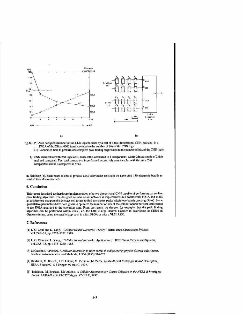
Neighbor

N6 N4 N2 N0

N, N, N, N,

c6 c,. c, c„

c. ifflitr' tell C, Cj C, C,

k—=-=1 > parallel

a) b)

fig.4a). (*) Area occupied (number of the CLB logic blocks) by a cell of a two-dimensional CNN, realized in a FPGA of the Xilinx 4000 family, related to the number of bits of the CNN logic.

(+) Elaboration time to perform one complete peak finding step related to the number of bits of the CNN logic.

b). CNN architecture with 2bit logic cells. Each cell is connected to 4 comparators; within 24ns a couple of 2bit is read and compared. The total comparison is performed recursively over 4 cycles with the same 2bit comparators and it is completed in 96ns.

in Hamburg [4]. Each board is able to process 12x8 calorimeter cells and we have used 130 electronic boards to read all the calorimeter cells.

6. Conclusion

This report described the hardware implementation of a two-dimensional CNN capable of performing an on-line peak finding algorithm. The designed cellular neural network is implemented in a commercial FPGA and it has an architecture mapping the detector cell arrays to find the cluster peaks within one bunch crossing (96ns). Some quantitative parameters have been given to optimize the number of bits of the cellular neural network cell related to the FPGA area and to the evolution time. From the results we deduce, for example, that the peak finding algorithm can be performed within 25ns , i.e. the LHC (Large Hadron Collider in costruction at CERN in Geneve) timing, using the parallel approach in a fast FPGA or with a VLSI ASIC.

7. References

[1] L. O. Chua and L. Yang, "Cellular Neural Networks: Theory," IEEE Trans.Circuits and Systems, Vol.CAS-35, pp. 1257-1272,1988.

[2] L. O. Chua and L. Yang, ' 'Cellular Neural Networks: Applications,'' IEEE Trans.Circuits and Systems, Vol.CAS-35, pp. 1273-1290,1988.

[3] M.Casolino, P.Picozza, A cellular automaton to filter events in a high energy physics discrete calorimeter, Nuclear Instrumentation and Methods, A 364 (1995) 516-523.

[4] Baldanza, M. Bruschi, I. D~ Antone, M. Piccinini, M. Zuffa, HERA-B Ecai Pretrigger Board Description, HERA-B note 97-178 Trigger 97-013 C, 1997.

[5] Baldanza, M. Bruschi, I.D~ Antone, A Cellular Automaton for Cluster Selection in the HERA-B Pretrigger Board HERA-B note 97-177 Trigger 97-012 C, 1997.

448

2000 6™ IEEE International Workshop on Cellular Neural Networks and Their Applications Proceedings

m-dimensional DT-CNN Implementation via Nested Lower Dimensional Architecture.

Alessandro Marongiu and Valerio Cimagalli Interuniversity Center for Research on Cognitive Processing in Natural and Artificial Systems

and Department of Electronic Engineering - "La Sapienza" University

Via Eudossiana 18,00184 - Rome (Italy) e-mail {marongiu, cima}@die.ing.uniromal.it

ABSTRACT: The development of the Cellular Neural Network (CNN) paradigm, and its wide use in many application fields, has shown that CNN is a complementary, and in some cases alternative, approach to classical computing machines. Despite their theoretical success, CNN VLSI implementations still suffer from size and dimension limitations. In fact, while the biggest CNN chips, due to VLSI constraints and to planar technology, have no more than few thousands of cells arranged on a 2D array, real problems may require millions of cells and may be multidimensional. In this paper we focus on the implementation of an m-dimensional DT-CNN with a limited number of lower (m-i)-dimensional DT-CNN circuits. As the target dimension is (m-i), we choose i = m-2 or i = m-1 in order to obtain an architecture using 2D or ID DT-CNN circuits which were proven to be feasible.

1. Introduction.

Since their introduction, Cellular Neural Networks (CNNs) have been constantly developed to include a broad class of problems arising in such fields as signal and image processing, pattern recognition, feature extraction and so on [1]. Such theoretical improvements have made the CNN an effective framework for (local) computational intensive applications. In fact, it has been demonstrated that CNN circuits, due to their intrinsic parallelism, exhibit very high computation power with respect to standard DSP-based computers [2]. Despite their theoretical success, CNN VLSI real implementations still suffer from size and dimensional limitations. In fact, while the biggest CNN chips, due to VLSI constraints, have no more than few thousands of cells distributed on a 2D or ID array [3] [4], real problems, such as Partial Differential Equations (PDE) solving, moving image processing and so on, may be multi-dimensional and may require millions of cells. While, in the next future, the VLSI sub-micron technology improvements will allow the implementation of CNN circuits with higher density cell arrays, the dimensionality limit of 2D will still remain due to the planar VLSI technology.

hi order to overcome dimensionality limitations, in this paper we introduce an effective methodology to implement an m-dimensional DT-CNN through a limited number of interconnected (m-i)-dimensional DT-CNN circuits. By choosing i = m-1 (i = m-2), the global architecture is composed of only ID (2D) DT-CNN circuits which were proven to be feasible and can be so considered as standard blocks. The main idea, underlying this work, is based on the realization of an m-dimensional DT-CNN with a limited number of (m-l)-dimensional DT-CNN- Then, in a recursive way, each individuated (m-l)-dimensional DT-CNN is realized with a limited number of (m-2)-dimensional DT-CNN and so on, until a 2D or ID dimension is reached. The paper is structured as in the following. In section 2 DT-CNN basic definitions are recalled, in section 3 the implementation of an m-dimensional DT-CNN with a (m-l)-architecture is considered. Then, in section 4, the application of the basic methodology in a recursive fashion is shown, and finally, in section 5, conclusions and future work are presented.

2. DT-CNN Basic Definitions. An m-dimensional DT-CNN, as was firstly introduced in [5], is algorithmically defined by the following

recurrence equations: X„(0,Zm Z2,Z,)=X*,o(Zm Z2,Z,)

r r r

Xjj,2„ Z2,Zt)= X -X X AJ&" *S.*lW*»('-l.Z«+*».-,%+fe»Z|+*l)) +

km=—r k%=—r *i=-r

r r r

+ X ••• X X .*«(*»> •■■>** *•>"-(''z-+*»> ■■•• z*+ki>Zi+ti)+' (1)

*«—r *2"-r*i=-r

where:

0-7803-6344-2/00/S10.00 ©2000 IEEE 449

- / is the integer-valued time; we suppose that 0 £ (£ T where T is the number of steps required to reach the steady state;

- (z„ ...z2z,)r is the cell coordinate m-vector representing DT-CNN cell C(z„, ...,z2, z,). DT-CNN cells are usually organized on a m-dimensional array, i.e. 0£z,<.Nr\ (i = 1,2,...,m) where Nt is the number of cells along the i-th dimension. Different network shapes are also allowed;

- (km ... k2k{) is the coordinate displacement m-vector used in the convolution operation. Am{km k2, kt) (Bm(km,..., k2, £,)) represents the feedback (control) template which is the kernel of the convolution operation on the state (input) values (the suffix m indicates m-dimensional templates). Templates are defined as m-dimensional arrays with (2r+l)* elements where r is the template radius. All cell interactions are within the radius r and so -r£k,<,r. Am(-) (Bm()) represents the whole m-dimensional feedback (control) template. Am(km,k„.lt ...,k„_i+u-) (B„(k„,kmA, ...,km.M,-)) is the (m-i')-dimensional feedback (control) template obtained by fixing the first i coordinates of /*„(•) (#„(•)).

- xm(t,z„ Zi,z,) is the state value of cell C(z„, ...,z2,zt) at time I where the suffix m indicates an m-dimensional state. xm(t,-) is the DT-CNN state of the whole network. x„(r, z„,z„,_,,..., z„_,*i, •) is the (m-i')-dimensional state obtained by fixing the first i coordinates of xm(l,-);

- «„(;, z„, ...,z2, Zi) is the input of the cell C(zm, ...,z2, z,) at time t where the suffix m indicates an m-dimensional input. u„((,) is the DT-CNN input of the whole network. um(t,zm,zm., z„.,t„ •) is the (m-i)-dimensional input obtained by fixing the first i coordinates of ujt,-);

- I is a bias value; - /is a sigmoid-like function and DT-CNN output at time (is %,((,-) =fixjj,-)).

The basic computation carried out by DT-CNN in one time step is the m-dimensional convolution performed on the output and input arrays. The block performing this basic computation is the one depicted in Figure I.

*„('->>•) ► A„fim(-),I

«JM H -> *„('.•)

Figure 1

The m-dimensional DT-CNN basic computation block receives, as inputs, the state at time t-\, x(l-\,), the input at time (, u(/,), and produces, as output, the state at time I, x(t,) computed according to (1). The m-dimensional DT-CNN basic computation block has an intrinsic parallelism and exhibits a very high computational power. Following [2], in each cell of the m-dimensional array are performed (2rf 1)"+1 computations (sum and multiply operations) for state convolution, and (2r+l)™+l for input convolution. Globally, in each cell 2(2rH)m+2 computations are executed in one time step. As the whole m-dimensional architecture has NmxNm.iX...X N, cells, the number of computations carried out by the global m-dimensional network is Ar„xAf„.,x...x Af,x[(2rf 1)"+I]x2 per time step. Supposing that the DT-CNN works at a frequency fw, the global number of Operations Per Seconds (OPS) is:

NmxNm.,x.. ,x N,x[(2r+1)"+1 ]x2xfw (2)

As an example, supposing a 3D square DT-CNN with 20 cells per side, r=\ andfw= 1MHz [6], we obtain 448 GigaOPS.

3. m-dimensional DT-CNN Implementation through a (m-l)-dimensional Architecture. Equation (1) can be rewritten as:

r T r /•

x„(t,zm ...,z2,z,)= £( X -X X ML,--,k2,kl)f{xdl-Uzm+km,...,z2+k2,z1+k1y) + km=-r *„-!=-'' *2=-rft,=-r

r r r

+ E -I E Bm(km,...,k2,k,)um(t,zm+km...,z2+k2,z,+k>) )+/ (3)

According to (3), the m-dimensional DT-CNN basic computation can be performed by means of the summation on km of the results of a (m-l)-dimensional DT-CNN basic computation. An architecture implementing the m-dimensional DT-CNN basic computation, using (2r+l) (m-l)-dimensional DT-CNN basic computation blocks, is depicted in Figure 2.a.

450

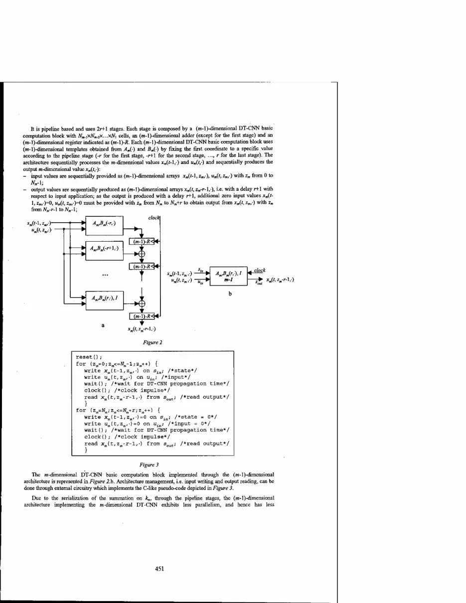
It is pipeline based and uses 2rH stages. Each stage is composed by a (m-l)-dimensional DT-CNN basic computation block with NmAyNm.2x.. .x/V, cells, an (m-l)-dimensional adder (except for the first stage) and an (m-l)-dimensional register indicated as (m-\)-R. Each (m-l)-dimensional DT-CNN basic computation block uses (m-l)-dimensional templates obtained from Am() and Bm() by fixing the first coordinate to a specific value according to the pipeline stage (-r for the first stage, -r+l for the second stage, ..., r for the last stage). The architecture sequentially processes the m-dimensional values x„(f-l,) and »„(/,•) and sequentially produces the output m-dimensional value x„(t,-): - input values are sequentially provided as (m-l)-dimensional arrays xm(t-\, zm,-% ujt, zm-) with z„ from 0 to

Nm-\; - output values are sequentially produced as (m-l)-dimensional arrays xm(t, zm-r-\,), i.e. with a delay r+\ with

respect to input application; as the output is produced with a delay r+l, additional zero input values xj^t- 1, z„,)=0, ujt, z„,)=0 must be provided with zm from Nm to Nm+r to obtain output from xm(t, zm,-) with zm

from N„-r-\ to JV„-1;

clock

".('.Z».0 > AM-',)

H > A„#m(-r+\,)

1 (m- >J?<K

-+0

WJr.-).'

(m-\)-R<H-

-♦O I (m-i)-j?<HJ

xm(r,zm-r-l,-)

Figure 2

reset () ; for (zB=0; zm<=Wm-l;2 .++) {

write x Jt-l,zml- on S, : /♦state*/ write u m(t,zm,-) on uin; /*input*/ wait(); /*wait f Dr DT-CNN propagation time*/ clock!) ; /»clock impulse* / read xm }

for (z„=Nm

(t,zm-r-l, ■) from s out; /»read output* /

;zln<=Nnl+r; z„++) { write x Jt-l,zm,- = 0 on si ; /*state = 0*/ write u ■ <t.*„.-> = 3 on uin; /»input = 0*/ wait () ; /*wait f or DT-CNN propagation time*/ clock () ; /*clock impulse* / read xm }

(t,zm-r-l, •) from s mc; /*read output*/

Figure 3

The m-dimensional DT-CNN basic computation block implemented through the (m-l)-dimensional architecture is represented in Figure 2.b. Architecture management, i.e. input writing and output reading, can be done through external circuitry which implements the C-like pseudo-code depicted in Figure 3.

Due to the serialization of the summation on k„, through the pipeline stages, the (m-l)-dimensional architecture implementing the m-dimensional DT-CNN exhibits less parallelism, and hence has less

451

computational power than the original DT-CNN. The (m-l)-dimensional architecture has intrinsic parallelism due to the (2r+l) DT-CNN (m-l)-dimensional basic computation blocks. From (2) each stage has a computational power Nm.,x...x A^,x((2r+l)"''+l)x2x/V OPS. Being the number of pipeline stages 2r+l we globally obtain (2r+ l)x7V„.,x...x N,x((2rt-l)m-l+l)x2xfw OPS. As an example, supposing a 3D square DT-CNN with 20 cells per side, r=] and fw = 1MHz, implemented through a 2D architecture, we have 3x2O2xl0x2xlMHz = 24 GigaOPS.

4. M-dimensional DT-CNN implementation through a (m-i>dimensional Architecture.

The methodology presented in section 2 can be used in a recursive way. in order to implement an m-dimensional DT-CNN basic computation block through a generic (m-i')-dimensional architecture. In fact: - the m-dimensional DT-CNN basic computation block is implemented by means of 2r+1 pipeline stages each

of them composed by a (m-l)-dimensional DT-CNN basic computation block with Arm_,x...xJV, cells, a

(m-l)-dimensional adder (except for the first stage) and a (m-l)-dimensional register composed by Nm.iX...xN, memory cells (see Figure 2). The architecture has (m-l)-dimensional I/O;

- each of the previous individuated (m-l)-dimensional DT-CNN block is implemented by means of 2r+l pipeline stages each of one is composed by a (m-2)-dimensional DT-CNN basic computation block with Nm.2X...xNt cells, a (m-2)-dimensional adder (except for the first stage) and a (m-2)-dimensional register composed by A^x.^xAf,. Each of the previous (m-l)-dimensional register is implemented through N„A+r+ 1 cascaded (m-2)-dimensional registers each of one having Nm,iX...xNl memory cells. Finally each of the previous (m-l)-dimensional adder is substituted with a (m-2)-dimensional one. The global architecture is composed by (2rH)2 (m-2)-dimensional DT-CNN basic computation blocks with Afm.2x...xJV| cells, and has (m-2)-dimensional I/O;

- each of the previous individuated (m-j'+l)-dimensional block is implemented by means of 2r+\ pipeline stages each of one being composed by a (m-/)-dimensional DT-CNN basic computation block with Nm.,x.. .xN, cells, a (m-i')-dimensional adder (except for the first stage) and a (m-0-dimensional register. Each of the previous (m-/+l)-dimensional registers is implemented through Nm_n.,+r+l cascaded (m-i')-dimensional registers each of one having ATm.,x...xJV, memory cells and, finally, each of the previous (m-i'+l)-dimcnsional adder is substituted with a (m-i)-dimensional one. The global architecture is composed by (2r+l)' (m-0-dimensional DT-CNN basic computation blocks with N„_jx.. .xN, cells, and has (m-0-dimensional I/O;

Notice that, despite at each recursion step the number of registers increases due to the implementation of a (m-i'+l)-dimensional register through Nm.M+r+l cascaded (m-/)-dimensional registers (for data synchronization with the subsequent stage), the global amount of memory remains almost the same. In fact, given a (m-i'+ l)-dimensional register composed by Nm.ltlxN„.,...xN, memory cells, after application of the methodology we have JV„.,t,+r+l registers with NmjX...xNt memory cells. Provided that N„^t, »r the global number of memory cells is almost the same.

The m-dimensional DT-CNN basic computation implemented with a generic (m-i')-dimensional architecture is represented by the block of Figure 4. Architecture management can be done through external circuitry implementing a C-like pseudo-code obtained by the nesting of the codes related to each recursion step as depicted in Figure 5.

m-i ■*•*»('.*»-'-I z„-M-r-U)

Figure 4

Due to the serialization of the summations on km, km_ , A„.m, the (m-/)-dimensional architecture has less parallelism than the original DT-CNN that causes performance decreasing. In fact, being the (m-i')-dimensional architecture composed of (2rH)' (m-/)-dimensional basic computation block, from (2), it performs (2rH)'xArmJx...xAM(2r+l)'"-'+l)x2x/fF OPS.

In order to obtain a VLSI feasible architecture, i must be chosen as i = m-\, obtaining a ID architecture, or '= m-2, obtaining a 2D architecture. ID architecture is easier to implement because interconnections design (and hence chip routing) between ID DT-CNNs is straightforward, but suffers from speed limitations because it exploits less parallelism with respect to the 2D architecture. On the contrary 2D architecture has higher

452

computational power but it is more difficult to implement because of the interconnections design between 2D DT-CNNs.

reset 0;

for (z„-0;Z.<-H-l;Z.-»-t> { for (z-.1-0;Za.1<-^a.1-l;z-.1++) {

for (Z-.i+i-0;Z11.J+1<-H1.i+1-l;ZB.ItJ++) { write x.(t-l,z.,z..1,..,z..„1,) on »,„; write nlt.1,1,.,,.,^,-1 on uln; wait() ; Clock() ;

read x.( t,z.-r-l,zB_,-r-l,_, z.^-r-l,) from «ou

' for <z.-i«- t-i.ii"..j.i<-1-i.i«i«.-i.i**l ( write x-(t-l,zil,z-.1,._,zM.Jtl,-}-0 on s^;

write ^ICi^iVi'-'^i.!'''"0 on uin<* wait(); clock 0i read xB( t, zB-r-l, zB_j-r-l,...( zB_i+1-r-l,-} from sou

for (z..,-H,.,;Z..1<-K..1tr;z1,.1++) {

for (z..,.1-0;z..1,1<-H,.i.1*r;Z..i„tt) { write xn(t-l,z(l,zn.1,._,za.itl,-)-0 on s^; write uB(t.zB, zB_1(..., z^.^,0 »0 on u^; waitO; clock!); read xB(t,zB-r-l,zn 1-r-l,._,z(t i+1-r-l,-) from sOL

}

for (z^JJ^j-z^-W^+r/z^+t) { for (zB.1"0;zI1.1<"W1]].1+r;zll].1++} {

£or <z-i-i-°;!t..i.i<-t-i.i*r''z.-l.i'f*I f write xB(t-l,zB,zB.1,*)-0 on sin; write uB{t,zB,zB j,-)-0 on u^; wait (I,■ clock!); read xB!t,zB-r-l,zB.1-r-l,-) from sou

Figure S

As an example of application of the previous methodology a 3D DT-CNN basic computation is implemented firstly with 2D architecture, then with ID architecture. Suppose the 3D DT-CNN has 20x20x20 cells, r= 1 and fw= 1MHz; From (2) it exhibits a computational power of 448 GigaOPS. Implementation with a 2D architecture gives the schematic depicted in Figure 6.a where each DTCNN basic computation block has 20x20 cells. Circuit management is done through an external circuitry implementing the C-like pseudo code of Figure 6.b. The global computational power of the resulting architecture is 3x202xl0x2xlMHz = 24 GigaOPS.

x3(M,z3,)-

«3C-I.V) !fiL-.

> -MJV-1,-)

A,ß3(0,)

> KfiJr,W

clock

2-R <K

■*o

2-R <K-

"►O

I 2-g <KJ

x3(/,z3-r-l,)

reset () ; for (z3=0;z3<=19,-z3+ + ) {

write x3(t-l,z3,-) on sisl; write u3(t,z3,-) on uin; clock () ,- waitO ; read x3(t,z3-2,-) from soul

} for (z3=20;z3<=21;z3++)

write x3( t-1, z3,-) =0 on si

write u3(t,z3,')=0 on uin; clock () ; waitO ; read x3(t,z3-2,-) from soul

}

Figure 6

Iterating the methodology we implement each of the previous individuated 2D DT-CNN basic computation block with a ID architecture obtaining the schematics of Figure 7.a. Each ID DT-CNN circuit has 20 cells. Circuit management is done through an external circuitry implementing the C-like pseudo code of Figure 7,b. From (2) the computational power of the ID architecture is 9x20x4x2x1MHz OPS = 1,44 GigaOPS.

5. Conclusions.

Due to the planar VLSI technology the CNN chips are usually implemented as 2D or ID array of cells. Some problems arising in such field as Partial Differential Equation (PDE) solving, moving image processing and so on, may be multidimensional problems which are intractable with 2D or ID CNN chips. In this paper we introduced a methodology to implement a m-dimensional DT-CNN with a limited number of lower dimensional blocks. Such lower dimensional blocks are usually 2D or ID blocks that were proven to be feasible. The resulting

453

architecture has less computational power than the original one, but it can be implemented in VLSI technology

exploiting both the internal DT-CNN and the pipeline parallelism, so giving high sustained computational

performances.

a3(f,Zj,V)'

reset () ; for {z3=0;z3<=19;z3++) {

for (z2 = 0;Z2< = 19; z2 + +) { write x3( t-l,z3, z2,-) on Bin; write u3( t, z3,z2,-) on uin; wait () ; clock (); read x3 (t, z3-2, z2-2,-) from sout;

) for (z2 = 20; z2<=21/z2 + + ) {

write x3{ t-1, z3, z2,0 =0 on ein; write u3 (t, z3, z2,-) =0 on uJn; wait () ; clock () ; read x3 {t, z3-2, z2-2,-)<=0 from sol

for (z3=20;Z3<-21;Z3++) { for (z2 = 0;Z2< = 21,*z2 + + ) {

write x3 (t-1, z3, z2,-) «=0 on sifJ; write Uj( t, z3,z2,-)=0 on uin; waitO ; clock (); read x3 (t, z3-2, z2-2,-) from eot

}

22 I-J; <Jt^ b

x3((^3-2,z2-2,-) Voui

Figure 7

References [ 1 ] L.O.Chua, T.Roska, "The CNN Paradigm", IEEE Transactions on Circuits and Systems, Vol. 40, No. 3, pp.

147-156, March 1993.

[2] L.O.Chua, T.Roska, T.Kozek, A.Zarandy, "CNN Universal Chips Crank Up the Computing Power", IEEE

Circuits & Devices, Vol. 12, pp. 18-28, July 1996.

[3] A.Rodriguez-Väzquez, S.Espejo, R. Dominguez-Castro, G.Linän, "The 64x64 Analog Input CNN Universal

Machine Chip and its ARAM', Proc. of Int. Symp. Nonlinear Theory and its Applications (NOLTA '98), pp. 667-670, 1998.

[4] M.Salerno, F.Sargeni, V.Bonaiuto, "A 6x6 Cells Interconnection-Oriented Programmable Chip for CNN",

Analogue Integrated Circuits and Signal Processing, Kluwer Academic Publisher, Vol. 15, No. 3, pp. 239- 250, March 1998.

[5] H.Harrer and J.A.Nossek, "Discrete Time Cellular Neural Networks", International Journal of Circuit

Theory and Applications, Vol.20, pp.453-467, 1992

[6] H.Harrer, J.A.Nossek, T.Roska, L.O.Chua, "A Current-Mode DTCNN Universal Chip", IEEE International

Symposium on Circuits and Systems 1994 (ISCAS 94), pp. 135-138, 1994

454

2000 6™ IEEE International Workshop on Cellular Neural Networks and Their Applications Proceedings

A Cellular Neural Networks Approach to Flame Image

Analysis for Combustion Monitoring

Bertucco L.0), Fichera A.(2), Nunnari G.(l), Pagano A.(1)

(1) Dipartimento Elettrico, Elettronico e Sistemistico, Universita di Catania Viale A. Doria, 6,95125 - Catania, Tel. +95-7382306, Fax +95 330793,

e-mail: apagano@ift.ing.unict.it, libert@dees.unict.it

(2) Istituto di Fisica Tecnica, Universita di Catania Viale A. Doria, 6,95125 - Catania, Tel. +95-7382450, Fax +95 337994,

Abstract - This paper proposes an approach based on Cellular Neural Networks (CNNs) to the analysis of flame images for real time monitoring of combustion process in a -waste incinerator. The use of CNNs analysis is dictated by the high images sampling rate, which was necessary due to the fast dynamics of the process in study. The dynamical behavior of the descriptors of the images processed by the CNNs was also studied and the results of this analysis are also presented

1. Introduction

It is well known that the fulfillment of actual energetic needs is mainly demanded to combustion processes of various kinds, which are prone to produce great amounts of highly polluting emissions (in particular CO and NO„). The introduction in the last years of increasingly stringent regulations on combustion emissions has pointed out the importance of monitoring and controlling combustion processes in order to optimize their performances.

One of the most powerful tools for monitoring combustion process is based on the measure of the flame front heat release. Many evidences show that the light intensity of the flame front is proportional to combustion rate and hence to heat release [1-2]. In fact, light is emitted by highly unstable chemical intermediate radicals, which can exist only in the reaction front. As a consequence, measures of light emitted by flames are the most common way of detecting heat release in combustion processes [3-4]. The heat release rate distribution depends on the flame structure and evolution and determines the distribution of temperature.

The heat release measurements and the study of temperature distribution inside combustion chambers is often performed by means of flame image analysis [5-6]. In fact, this approach allows to detect the oscillating behavior of the structure of the flame (vortices) and the existence of hot spots, i.e. restricted regions of the flame characterized by high temperatures which may cause the rising of CO and NOx emissions. The main drawback of the classical analysis based on image processing approach, is that it requires large amount of data to be processed. Moreover, due the fast dynamics of combustion systems, flame images analysis has been used for off- line studies of combustion but is difficult to apply in real-time monitoring of combustion processes.

This paper presents an innovative approach to the analysis of flame images detected on a waste incinerator combustion plant for thermal power production based on Cellular Neural Networks (CNNs). In fact, CNNs are particularly able to perform real time image analysis and hence they can be effectively used in monitoring and controlling combustion process, overcoming the drawbacks previously mentioned.

2. Cellular Neural Networks Approach

In the present work a sequence of frames detected from a waste incinerator combustion chamber was analyzed. The incinerator plant is placed in the outskirts of Ferrara and, together with a geothermal plant, provides the 37.5% (corresponding to 45000 Gcal/year) of the whole heat power requested for civil use. The sequence was acquired using a ultrafest videocamera, able to pick up to 800 frames per second, which was operated at a sampling rate of 250 Hz (i.e. 250 frames per second). Each frame is a gray scale image made of 32x32 pixels. It must be noticed that the sampling frequency is indeed too high to perform real time flame image analysis using any of the traditional approaches.

On the other hand CNNs image processing is extremely fast, and therefore it can be particularly useful for the

0-7803-6344-2/00/$10.00 ©2000 IEEE 455

application herein proposed, in which 250 frames must be elaborated each second. Moreover many different operations can be performed simply modifying a few parameters of the cloning templates [7-8] of the CNNs; in other words, the proposed approach offers great flexibility and allows real time flame image analysis.

The present study was carried out using a CNN software simulator, described in [9]. The operations performed on the images are implemented using linear templates and a single layer CNN.

Figure 1 (a) presents the image of the flame detected by the videocamera. In mis figure the central clear region represents the flame burning the fuel emitted by the injector placed around the centerline of the bottom of the figure. The smaller clear spots on both sides of the figure are parts of the flames produced by two injectors surrounding the central one.

The first step of the analysis consisted of thresholding the gray scale images. In order to do this it is necessary to threshold each pixel of the original image. This can be simply done by setting to white those pixels characterized by gray levels greater than the threshold and to black all the other. The templates used to perform such an operation are called Threshold templates [10]. The choice of the threshold is very important as it corresponds to choose a light emission intensity, which plays a specific role in combustion processes monitoring.

Fig. I (a) Original Image (b) Threshold Image

In feet, the light intensity of the flame front is proportional to combustion rate and hence to heat release [1-2]. In other words, measure of light intensity can be used to localize the core of the flame. The core is the region of the flame reaching high temperature levels in which combustion mainly occurs; the flame front separates this region by the exhausted gas and assume the structure typical of combustion vortices. This structure is characterized by different temperature levels depending on the progressive mixing of the burning gas with the exhausted gas. Therefore, thresholding the images can be used either to determine the core of the flame or to detect hot spots, i.e. regions characterized by temperatures higher than a specified value. In both cases it is necessary to opportunely choose the temperature threshold and the corresponding gray scale level.

In this work the threshold was chosen to allow the analysis of the structure of vortices, basing on empirical considerations obtained from the observation of several sequences. Figure 1 (b) reports the image obtained thresholding the one of Fig. 1 (a) and indeed well describes the vortex produced by the central injector. Nevertheless, the image obtained applying only the threshold operator is in some way affected by the interference of the flames due to the lateral injectors. Moreover, the presence of isolated white pixels is in general due to very fest local combustion phenomena and can therefore be regarded as noise.

Both the problems were easily solved applying another typical CNNs operator, which consists in performing the logic AND (Images AND,) of N successive threshold frames (Images Th,„ i'=l,2, ... iV)as shown in Fig. 2(a). The output of this operator is the image resulting from the intersection of the set of white pixels of the N images (Fig. 2 (b)). The application of the logic AND, (performed by using AND templates [10]), to the case in study can be considered as a sort of image filter acting both on the pixels spatial distribution and on the temporal evolution of the flame image. Therefore, the choice of the number of frames N must be done considering both these actions. In the present study it was sufficient to apply the logic AND to four images (Step = 4).

Image Image Th, Th,

Image Ths

Image Th,

Image Th,

>\' /\u A^Nk < y Image AND,

Image AND,

Image AND,

(a) (b)

Fig. 2 (a) Sequence: AND Images Construction with Step=3 (b) AND Pixel

456

The images obtained applying the threshold and the logic And operator were used to describe die evolution of vortexes inside the combustion chamber. Fig. 3 (a) shows six gray scale images, which were selected by sampling a sequence of 90 frames and hence correspond to a time period of 0.28 seconds. Fig. 3 (b) reports the images obtained applying the threshold and the logic AND to the previous sequence.

Fig. 3 (a) Original images (b) Threshold + logic AND images

Fig. 3, reports a sequence that well represents the general behavior of several other sequences considered during this study. This sequence evidences the ability of the CNNs in describing the dynamical evolution of a vortex. Time evolution of this structure is characterized by the merging process [5], which consists of the periodical formation of a great scale vortex from the fusion of two small scale vortexes. This behavior cannot be revealed by the analysis of gray scale images but is evident in those processed by the CNN.

The analysis of vortex evolution is extremely important to reach a full insight of combustion phenomena In fact, the mechanism of vortex shedding and the interaction between vortexes govern pressure oscillations and heat release fluctuations related to CO and NO* emissions and to vibratory phenomena that can be harmful for the combustion chamber. In the next section an analysis of the complex dynamics characterizing vortex behaviors is addressed.

3. Analysis of Flame Dynamics

The dynamical behavior of the vortex was studied using the sequences processed according to the approach discussed in the previous section and consisting of the application of the logic AND operator to the threshold images. To this aim, for each of the images of the sequences the central moments, described in [11], were calculated. This step was necessary to reduce the study of the dynamical evolution of the flame to traditional time series analysis. Therefore, seven invariant moments, i.e. image descriptors, were calculated per each image

400 600

Frames

Figure 4 Comparison of the noisy and filtered time series for the first invariant moment of 1000 flame images

457

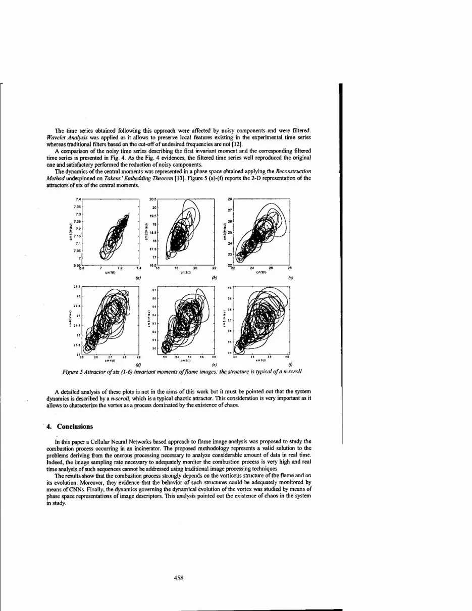
The time series obtained following this approach were affected by noisy components and were filtered. Wavelet Analysis was applied as it allows to preserve local features existing in the experimental time series whereas traditional filters based on the cut-off of undesired frequencies are not [12].

A comparison of the noisy time series describing the first invariant moment and the corresponding filtered time series is presented in Fig. 4. As the Fig. 4 evidences, the filtered time series well reproduced the original one and satisfactory performed the reduction of noisy components.

The dynamics of the central moments was represented in a phase space obtained applying the Reconstruction Method underpinned on Tokens' Embedding Theorem [13]. Figure 5 (a)-(f) reports the 2-D representation of the attractors of six of the central moments.

(a) (b) (c)

Figure 5 Attractor of six (1-6) invariant moments of flame images: the structure is typical of a n-scroll.

A detailed analysis of these plots is not in the aims of this work but it must be pointed out that the system dynamics is described by a n-scroll, which is a typical chaotic attractor. This consideration is very important as it allows to characterize the vortex as a process dominated by the existence of chaos.

4. Conclusions

In this paper a Cellular Neural Networks based approach to flame image analysis was proposed to study the combustion process occurring in an incinerator. The proposed methodology represents a valid solution to the problems deriving from the onerous processing necessary to analyze considerable amount of data in real time. Indeed, the image sampling rate necessary to adequately monitor the combustion process is very high and real time analysis of such sequences cannot be addressed using traditional image processing techniques.

The results show that the combustion process strongly depends on the vorticous structure of the flame and on its evolution. Moreover, they evidence that the behavior of such structures could be adequately monitored by means of CNNs. Finally, the dynamics governing the dynamical evolution of the vortex was studied by means of phase space representations of image descriptors. This analysis pointed out the existence of chaos in the system in study.

458

5. References

[I] John R. R. and Summerfield M, "Studies of the Mechanism of Flame Stabilization by a Spectral Intensity Method", Jet Propulsion, 25,535, 1995.

[2] John R. R. and Summerfield M, "Effect of Turbulence on Radiation Intensity from Propane-Air Flames", Jet Propulsion, 27,169,1957.

[3] McManus K- R-, Vandsburger U, Bowman C. T. "Combustor Performance Enhancement through Direst Shear Layer Excitation", Combustion and Flame, 82, pp.75-92,1990

[4] Padmanabhan K. T., Bowman C. T., Powell J. D., "An Adaptive Optimal Combustion Control Strategy", Combustion and Flame, 100, pp. 101-110,1995.

[5] Schadow K. C. and Gutmark E., "Combustion Instability Related to Vortex Shedding in Dump Combustors and Their Passive Control", Progress in Energy Combustion Science, 1992,18, pp. 117-132,1992.

[6] Poinsot T., Veynante D, Bourienne F., Candel S., Esposito E. Surget J., "Initiation and Suppression of Combustion Instabilities by Active Control", 22th Symp. (Intern.) on Combustion, The Combustion Institute, pp. 1363-1370,1988.

[7] Chua L. O. and Yang L., "Cellular Neural Networks: Theory", IEEE Transactions on Circuits and Systems Vol. 35, No. 10, pp. 1257-1272, October 1988.

[8] Chua L. O. and Yang L., "Cellular Neural Networks: Applications", IEEE Transactions on Circuits and Systems Vol. 35, No. 10, pp. 1273-1290, October 1988.

[9] Bertucco L. and Nunnari G., "A Multi-Layer Cellular Neural Network Simulator for Image Processing Applications", Proceedings of the Third International ICSC Symposia on Intelligent Industrial Automation IIA'99 and Soft Computing SOCO'99, pp. 147-151, Genova, Italy, June 1999,.

[10] Roska T., Kelt L, Nemes L., Zarandy A. and Szolgay P. CSL CNN Software Library (Templates and Algorithms) Vers. 7.3, Hungarian Academy of Sciences, Budapest (Hungary), August, 1999.

[II] Gonzalez R. C. and Woods R. E. "Digital Image Processing", 2nd edn. Addison-Wesley Publishing Company, pp.514-519,1993..

[12] R. K. Young, "Wavelet Theory and Its Applications, Kluwer Academic Publishers", Dordrecht, 1993, [13] Takens F., "Lecture Notes in Mathematics, Dynamical System and Turbulence", D. A. Rand & L. S.

Young, Springer, New York, 1981.

459

AUTHORINDEX

Acciani G., 141 Al-AniN.K.,87,235 Amenta C, 147 Arena P., 147,153,339

Baglio S., 147 BaldanzaC.,443 Balsi M., 135,363 BälyaD., 165 BertuccoL., 153,159,455 Bisi F., 443 BonaiutoV., 225, 273 Branciforte M., 333, 345 BreaV.M.,425 Brendel M., 93 Brucoli M., 369 Bruschi M., 443 BuczynskiB., 431

CabelloD.,363,425 CafagnaD., 369 Caponetto R, 153 Camimeo L., 369 Cheng C.R, 301 Chilton E., 315 ChuaL.O., 1,177,183,189,357 Cimagalli V., 449 Civalleri P.P., 247 Coli M., 295 Crounse K.R., 357 Csapodi M., 267 Czüni L., 51

Dabrowski A., 253 Dantone I., 443 DogaruR., 177,183,189 Domfnguez-CastroR., 201, 219,283,289 Dupret A., 207

Espejo S., 79,201,219,283,289

Fajfar I., 277 Fargione G., 159 Fichera A., 455 Földesy P., 79,219,283,289 Fortuna L., 147,153,339,345 FrascaM., 339

Gacsadi A., 99 Gal V., 105 Galias Z., 253 Garcia-Alegre M.C., 327,381

Gatt E., 315 Gilli M., 247 Giustolisi G, 333 Goras L., 27 Grassi G, 141 GrigatR.-R.,351 Guinea D., 327,381

Halonen K., 321,401,437 HänggiM., 177,183,189 Hegt H., 21 HeraultJ., 39 Hidvegi T., 9

Isoaho J.,229

Jankowski S., 431

KacprzakT., 87,235 Kananen A, 321 KekL.,79 Klein J.O., 207 Köneke A., 39 Kozma P., 9 KunzR, 123,129,241 Kuznetsov A.S., 413,419

LaihoM.,401 Linän G, 79,201,219,283,289 LoncarA., 123,129,17i Lopez P., 363

Maiorescu A., 27 Marongiu A., 449 Matsuyama M., 83 Meneghini S., 443 MerlatL., 39 MicallefJ., 315 Mladenov V., 21 Monnin D., 39 Mori M., 83,

Nakaguchi T., 57 Nemeth E., 15,165 NicotraV.,333 Nshare A., 207 Nuidel I.V., 45 Nunnari G, 153,159,455

Ogorzatek M, 253 Onishi M., 57 OrzoL., Ill

461

Paakkulainen J., 229 Xibilia M.G., 147, 345 Paasio A., 229, 321,401,437 Pagano A., 455 Yakhno V.G., 33,45 Palazzari P., 295 Yen W.C., 195 Palumbo G., 333 Yokosawa K., 407 Pellecchia A., 375 Perezowsky M., 351 Zanela A., 117,273, 375 PerkoM.,277 Zarandy A., 79,267 Petras I., 3 Zuffa M., 443 PleskaczW.,431 Porebska A., 309 Porto D., 153 Preciado V.M., 327,381 Puhan J., 277

Radvänyi A.G., 387 RekeczkyC, 15,79,213 Ribeiro A., 327, 381 Richiusa D„ 147 Risitano A., 159 Rizzi M., 443 Rodriguez-Vazquez A., 79, 201, 213, 219, 265, 283, 289 RoskaB., 15,165 Roska T., 3,73,79, 93,105,165,213,267 RughiR.,295

Saatci E., 63 Salerno M., 225,273 Sargeni F., 225,273 Serrano-GotarredonaT., 213 ShalfeevV.D.,413,419 Shi B.E., 69 Slavova A., 259 Strazzuso S., 345 Szatmäri I., 79,395 Sziränyi T., 51, 79 Szolgay P., 9, 79,99 Szolgay Z, 9

TanakaM., 57, 83,407 Tanji Y., 57, 83,407 TaragUoS., 117,273,375 Tavsanoglu V., 63 Teodorescu T., 27 TetzlaffR., 123,129,171,241 TumaT., 277

Vicente J., 327, 381 Vilarfflo D.L., 363, 425 VulloL., 147

Wee C, 357 Werblin F., 15,165 Wiehler K., 351 Wielgus A., 431 WiSniewskiM.,431

Wu C.Y., 195, 301

462