9.5 packet-switching principles - aula virtual

9.5 / PackeT-sWiTching PrinciPles 283

9.5 packet-switching principLes

The long-haul circuit-switching telecommunications network was originally designed to handle voice traffic, and the majority of traffic on these networks continues to be voice. A key characteristic of circuit-switching networks is that resources within the network are dedicated to a particular call. For voice connections, the resulting circuit will enjoy a high percentage of utilization because, most of the time, one party or the other is talking. However, as the circuit-switching network began to be used increasingly for data connections, two shortcomings became apparent:

• In a typical user/host data connection (e.g., personal computer user logged on to a database server), much of the time the line is idle. Thus, with data connec-tions, a circuit-switching approach is inefficient.

• In a circuit-switching network, the connection provides for transmission at a constant data rate. Thus, each of the two devices that are connected must transmit and receive at the same data rate as the other. This limits the utility of the network in interconnecting a variety of host computers and workstations.

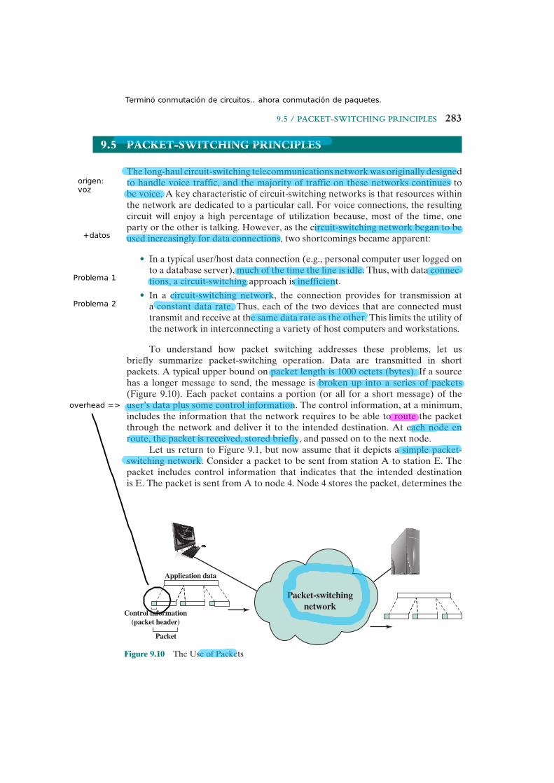
To understand how packet switching addresses these problems, let us briefly summarize packet-switching operation. Data are transmitted in short packets. A typical upper bound on packet length is 1000 octets (bytes). If a source has a longer message to send, the message is broken up into a series of packets (Figure 9.10). Each packet contains a portion (or all for a short message) of the user’s data plus some control information. The control information, at a minimum, includes the information that the network requires to be able to route the packet through the network and deliver it to the intended destination. At each node en route, the packet is received, stored briefly, and passed on to the next node.

Let us return to Figure 9.1, but now assume that it depicts a simple packet-switching network. Consider a packet to be sent from station A to station E. The packet includes control information that indicates that the intended destination is E. The packet is sent from A to node 4. Node 4 stores the packet, determines the

Application data

Control information(packet header)

Packet

Packet-switchingnetwork

Figure 9.10 The Use of Packets

Terminó conmutación de circuitos.. ahora conmutación de paquetes.

origen:voz

+datos

Problema 1

Problema 2

overhead =>

284 chaPTer 9 / Wan Technology and ProTocols

next leg of the route (say 5), and queues the packet to go out on that link (the 4-5 link). When the link is available, the packet is transmitted to node 5, which forwards the packet to node 6, and finally to E. This approach has a number of advantages over circuit switching:

• Line efficiency is greater, because a single node-to-node link can be dynami-cally shared by many packets over time. The packets are queued up and transmitted as rapidly as possible over the link. By contrast, with circuit switching, time on a node-to-node link is preallocated using synchronous time-division multiplexing. Much of the time, such a link may be idle because a portion of its time is dedicated to a connection that is idle.

• A packet-switching network can perform data-rate conversion. Two stations of different data rates can exchange packets because each connects to its node at its proper data rate.

• When traffic becomes heavy on a circuit-switching network, some calls are blocked; that is, the network refuses to accept additional connection requests until the load on the network decreases. On a packet-switching network, pack-ets are still accepted, but delivery delay increases.

• Priorities can be used. If a node has a number of packets queued for trans-mission, it can transmit the higher-priority packets first. These packets will therefore experience less delay than lower-priority packets.

Switching Technique

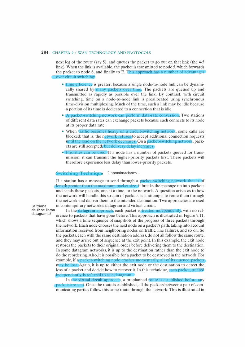
If a station has a message to send through a packet-switching network that is of length greater than the maximum packet size, it breaks the message up into packets and sends these packets, one at a time, to the network. A question arises as to how the network will handle this stream of packets as it attempts to route them through the network and deliver them to the intended destination. Two approaches are used in contemporary networks: datagram and virtual circuit.

In the datagram approach, each packet is treated independently, with no ref-erence to packets that have gone before. This approach is illustrated in Figure 9.11, which shows a time sequence of snapshots of the progress of three packets through the network. Each node chooses the next node on a packet’s path, taking into account information received from neighboring nodes on traffic, line failures, and so on. So the packets, each with the same destination address, do not all follow the same route, and they may arrive out of sequence at the exit point. In this example, the exit node restores the packets to their original order before delivering them to the destination. In some datagram networks, it is up to the destination rather than the exit node to do the reordering. Also, it is possible for a packet to be destroyed in the network. For example, if a packet-switching node crashes momentarily, all of its queued packets may be lost. Again, it is up to either the exit node or the destination to detect the loss of a packet and decide how to recover it. In this technique, each packet, treated independently, is referred to as a datagram.

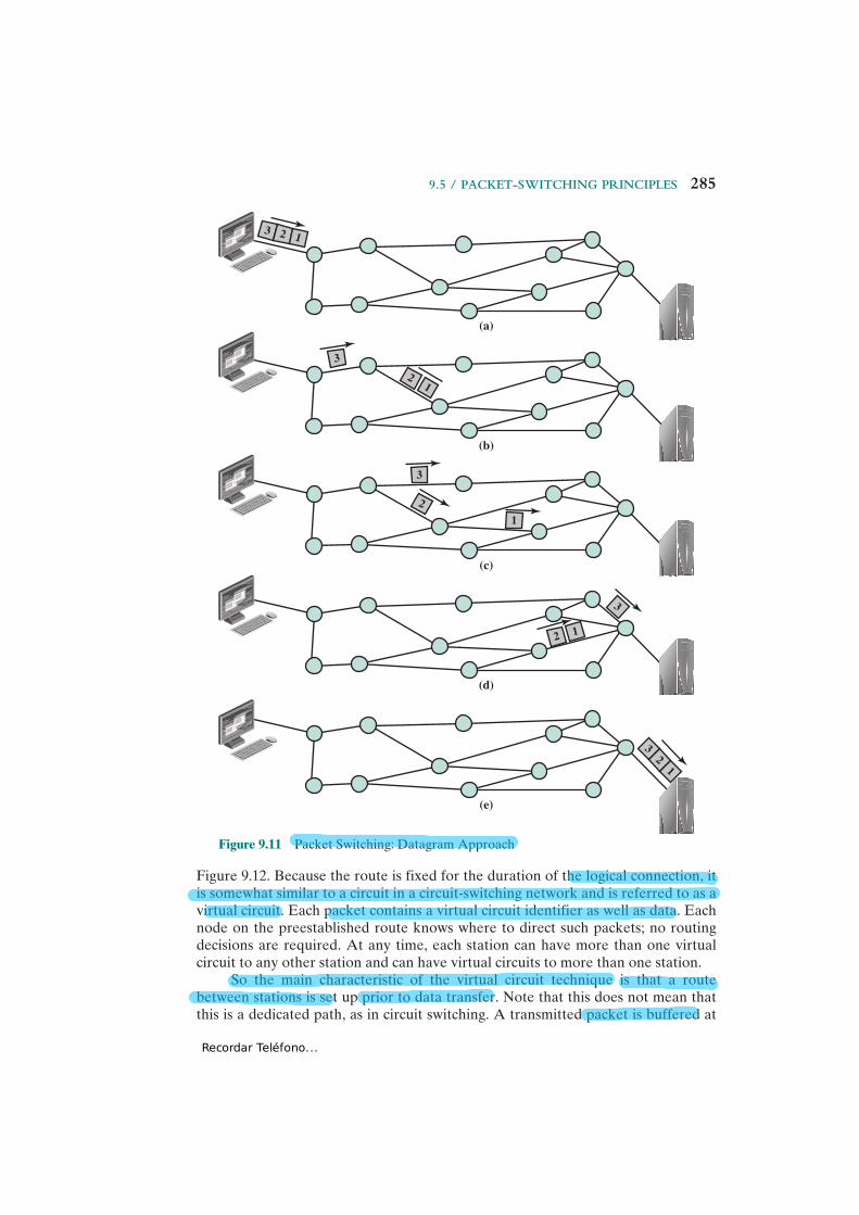
In the virtual circuit approach, a preplanned route is established before any packets are sent. Once the route is established, all the packets between a pair of com-municating parties follow this same route through the network. This is illustrated in

La tramade IP se llamadatagrama!

2 aproximaciones...


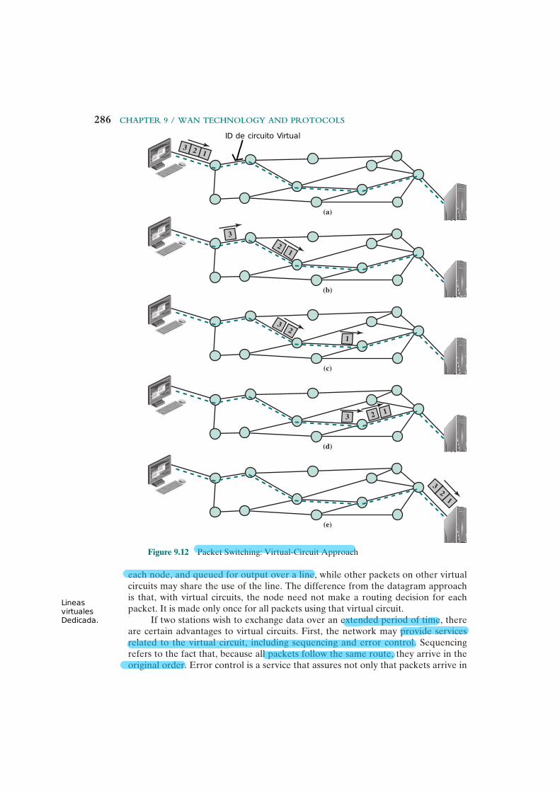
Figure 9.12. Because the route is fixed for the duration of the logical connection, it is somewhat similar to a circuit in a circuit-switching network and is referred to as a virtual circuit. Each packet contains a virtual circuit identifier as well as data. Each node on the preestablished route knows where to direct such packets; no routing decisions are required. At any time, each station can have more than one virtual circuit to any other station and can have virtual circuits to more than one station.

So the main characteristic of the virtual circuit technique is that a route between stations is set up prior to data transfer. Note that this does not mean that this is a dedicated path, as in circuit switching. A transmitted packet is buffered at

(c)

(b)

(a)

(d)

(e)

3

3

3

2

32

1

1

3

2

1

2 1

21

Figure 9.11 Packet Switching: Datagram Approach

Recordar Teléfono...


each node, and queued for output over a line, while other packets on other virtual circuits may share the use of the line. The difference from the datagram approach is that, with virtual circuits, the node need not make a routing decision for each packet. It is made only once for all packets using that virtual circuit.

If two stations wish to exchange data over an extended period of time, there are certain advantages to virtual circuits. First, the network may provide services related to the virtual circuit, including sequencing and error control. Sequencing refers to the fact that, because all packets follow the same route, they arrive in the original order. Error control is a service that assures not only that packets arrive in

(c)

(b)

(a)

(d)

(e)

3

3

2

21

32

1

3

32

1

2 1

1

Figure 9.12 Packet Switching: Virtual-Circuit Approach

ID de circuito Virtual

Lineasvirtuales Dedicada.


proper sequence, but also that all packets arrive correctly. For example, if a packet in a sequence from node 4 to node 6 fails to arrive at node 6, or arrives with an error, node 6 can request a retransmission of that packet from node 4. Another advantage is that packets should transit the network more rapidly with a virtual circuit; it is not necessary to make a routing decision for each packet at each node.

One advantage of the datagram approach is that the call setup phase is avoided. Thus, if a station wishes to send only one or a few packets, datagram deliv-ery will be quicker. Another advantage of the datagram service is that, because it is more primitive, it is more flexible. For example, if congestion develops in one part of the network, incoming datagrams can be routed away from the congestion. With the use of virtual circuits, packets follow a predefined route, and thus it is more dif-ficult for the network to adapt to congestion. A third advantage is that datagram delivery is inherently more reliable. With the use of virtual circuits, if a node fails, all virtual circuits that pass through that node are lost. With datagram delivery, if a node fails, subsequent packets may find an alternate route that bypasses that node. A datagram-style of operation is common in internetworks, discussed in Part Five.

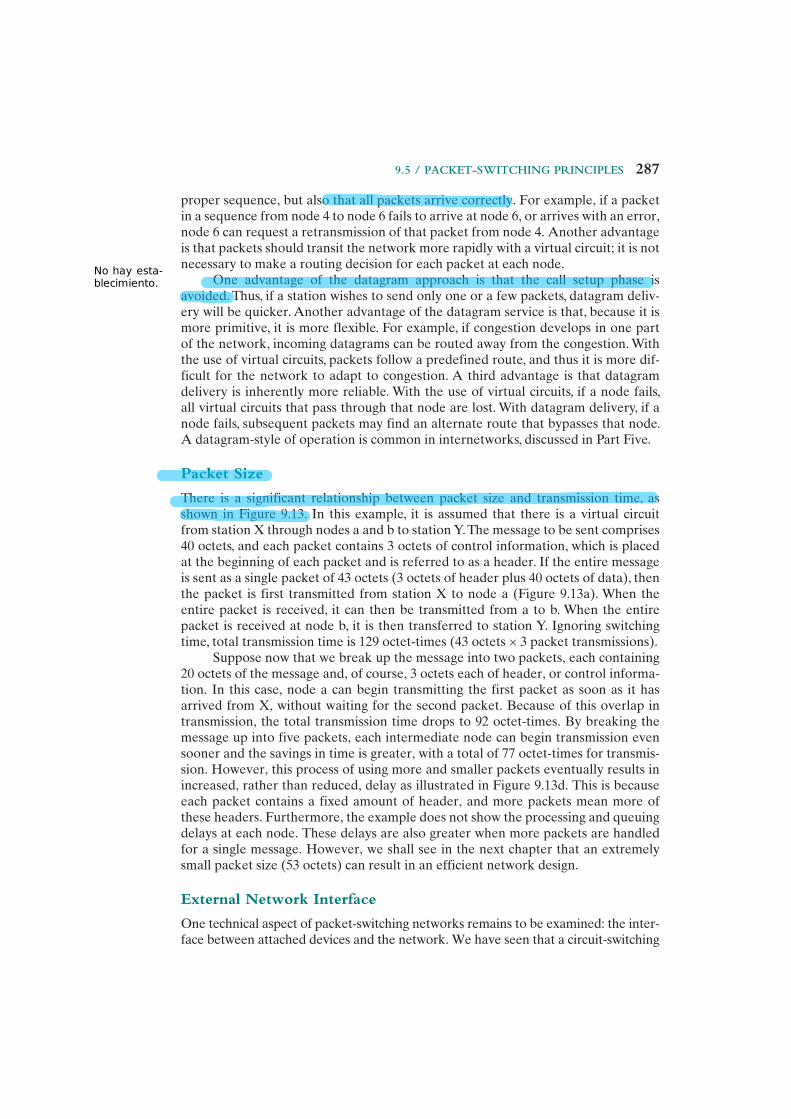
Packet Size

There is a significant relationship between packet size and transmission time, as shown in Figure 9.13. In this example, it is assumed that there is a virtual circuit from station X through nodes a and b to station Y. The message to be sent comprises 40 octets, and each packet contains 3 octets of control information, which is placed at the beginning of each packet and is referred to as a header. If the entire message is sent as a single packet of 43 octets (3 octets of header plus 40 octets of data), then the packet is first transmitted from station X to node a (Figure 9.13a). When the entire packet is received, it can then be transmitted from a to b. When the entire packet is received at node b, it is then transferred to station Y. Ignoring switching time, total transmission time is 129 octet-times (43 octets × 3 packet transmissions).

Suppose now that we break up the message into two packets, each containing 20 octets of the message and, of course, 3 octets each of header, or control informa-tion. In this case, node a can begin transmitting the first packet as soon as it has arrived from X, without waiting for the second packet. Because of this overlap in transmission, the total transmission time drops to 92 octet-times. By breaking the message up into five packets, each intermediate node can begin transmission even sooner and the savings in time is greater, with a total of 77 octet-times for transmis-sion. However, this process of using more and smaller packets eventually results in increased, rather than reduced, delay as illustrated in Figure 9.13d. This is because each packet contains a fixed amount of header, and more packets mean more of these headers. Furthermore, the example does not show the processing and queuing delays at each node. These delays are also greater when more packets are handled for a single message. However, we shall see in the next chapter that an extremely small packet size (53 octets) can result in an efficient network design.

External Network Interface

One technical aspect of packet-switching networks remains to be examined: the inter-face between attached devices and the network. We have seen that a circuit-switching

No hay esta-blecimiento.


network provides a transparent communications path for attached devices that makes it appear that the two communicating stations have a direct link. However, in the case of packet-switching networks, the attached stations must organize their data into pack-ets for transmission. This requires a certain level of cooperation between the network and the attached stations. This cooperation is embodied in an interface standard. The standard used for traditional packet-switching networks is X.25, which is described in Appendix U. Another interface standard is frame relay, also discussed in Appendix U.

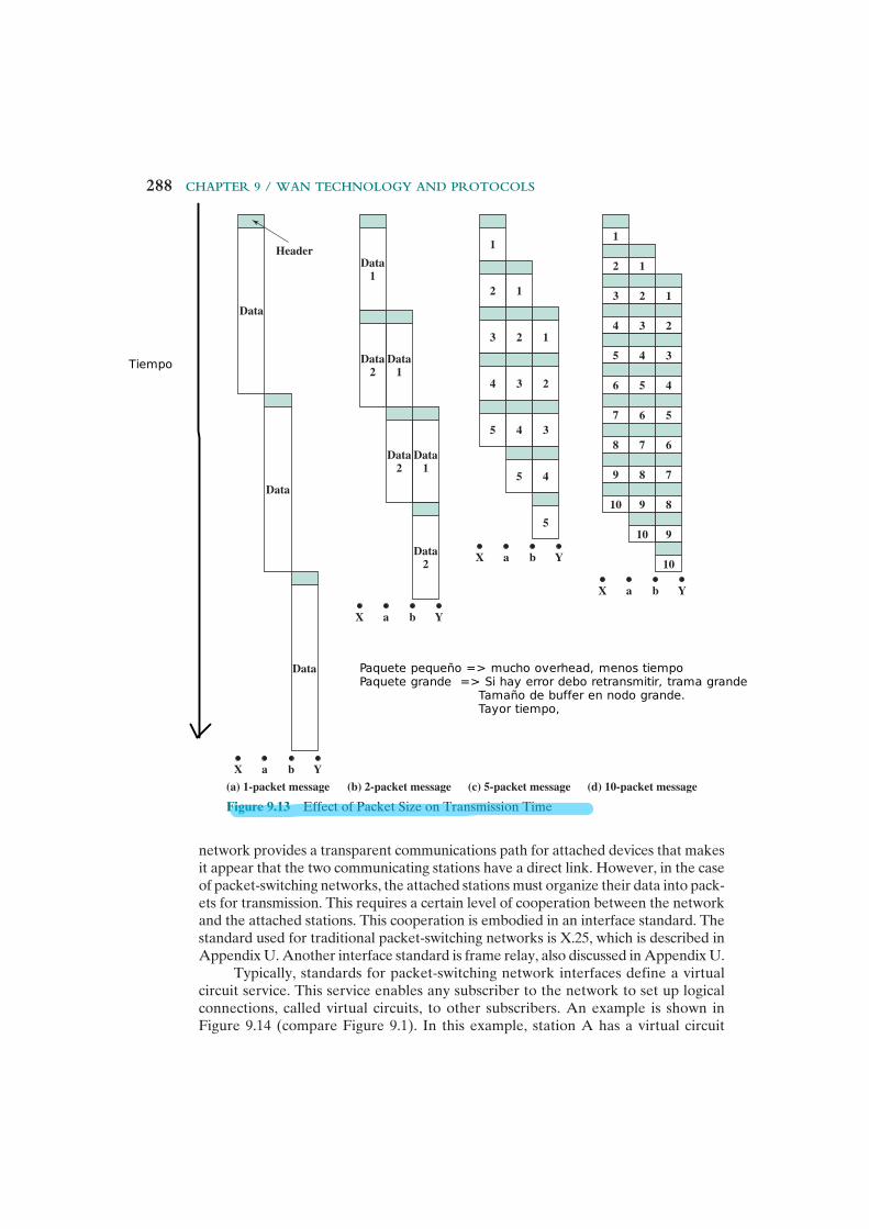
Typically, standards for packet-switching network interfaces define a virtual circuit service. This service enables any subscriber to the network to set up logical connections, called virtual circuits, to other subscribers. An example is shown in Figure 9.14 (compare Figure 9.1). In this example, station A has a virtual circuit

1

Data1

Data

Header

(a) 1-packet message (b) 2-packet message (c) 5-packet message (d) 10-packet message

Data

Data

Data2

Data1

Data2

Data1

Data2

1

2

3

4

5

6

7

8

9

10

1

2

3

4

5

6

7

8

9

10

1

2

3

4

5

6

7

8

9

10

2

3

4

5

1

2

3

4

5

1

2

3

4

5

X Yba

X Yba

X Yba

X Yba

Figure 9.13 Effect of Packet Size on Transmission Time

Paquete pequeño => mucho overhead, menos tiempoPaquete grande => Si hay error debo retransmitir, trama grande

Tamaño de buffer en nodo grande.Tayor tiempo,

Tiempo


connection to C; station B has two virtual circuits established, one to C and one to D; and stations E and F each have a virtual circuit connection to D.

In this context, the term virtual circuit refers to the logical connection between two stations through the network; this is perhaps best termed an external virtual circuit. Earlier, we used the term virtual circuit to refer to a specific preplanned route through the network between two stations; this could be called an internal virtual circuit. Typically, there is a one-to-one relationship between external and internal virtual circuits. However, it is also possible to employ an external virtual circuit service with a datagram-style network. What is important for an external virtual circuit is that there is a logical relationship, or logical channel, established between two stations, and all of the data associated with that logical channel are considered as part of a single stream of data between the two stations. For example, in Figure 9.14, station D keeps track of data packets arriving from three different workstations (B, E, F) on the basis of the virtual circuit number associated with each incoming packet.

Comparison of Circuit Switching and Packet Switching

Having looked at the internal operation of packet switching, we can now return to a comparison of this technique with circuit switching. We first look at the important issue of performance and then examine other characteristics.

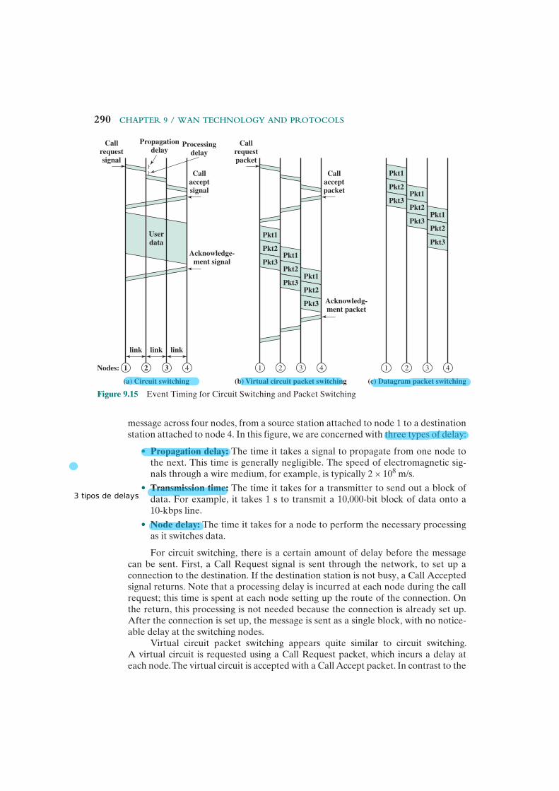
Performance A simple comparison of circuit switching and the two forms of packet switching is provided in Figure 9.15. The figure depicts the transmission of a

A

E

C

D

Personalcomputer

Personalcomputer

Mainframe

Personalcomputer

Personalcomputer

Server

Packet-switchingnetwork

Solid line = physical linkDashed line = virtual circuit

F

B

Figure 9.14 The Use of Virtual Circuits


message across four nodes, from a source station attached to node 1 to a destination station attached to node 4. In this figure, we are concerned with three types of delay:

• Propagation delay: The time it takes a signal to propagate from one node to the next. This time is generally negligible. The speed of electromagnetic sig-nals through a wire medium, for example, is typically 2 × 108 m/s.

• Transmission time: The time it takes for a transmitter to send out a block of data. For example, it takes 1 s to transmit a 10,000-bit block of data onto a 10-kbps line.

• Node delay: The time it takes for a node to perform the necessary processing as it switches data.

For circuit switching, there is a certain amount of delay before the message can be sent. First, a Call Request signal is sent through the network, to set up a connection to the destination. If the destination station is not busy, a Call Accepted signal returns. Note that a processing delay is incurred at each node during the call request; this time is spent at each node setting up the route of the connection. On the return, this processing is not needed because the connection is already set up. After the connection is set up, the message is sent as a single block, with no notice-able delay at the switching nodes.

Virtual circuit packet switching appears quite similar to circuit switching. A virtual circuit is requested using a Call Request packet, which incurs a delay at each node. The virtual circuit is accepted with a Call Accept packet. In contrast to the

2 3

(a) Circuit switching

Callrequestsignal

Callacceptsignal

Propagationdelay

Processingdelay

link

Nodes:

Acknowledge-ment signal

1 4

link link

Userdata

1 432

(b) Virtual circuit packet switching

Callrequestpacket

Callacceptpacket

Acknowledg-ment packet

Pkt2

Pkt3

Pkt1

Pkt2

Pkt3

Pkt1

Pkt2

Pkt3

Pkt1

1 432

(c) Datagram packet switching

Pkt2

Pkt3

Pkt1

Pkt2

Pkt3

Pkt1

Pkt2

Pkt3

Pkt1

Figure 9.15 Event Timing for Circuit Switching and Packet Switching

3 tipos de delays


circuit-switching case, the call acceptance also experiences node delays, even though the virtual circuit route is now established. The reason is that this packet is queued at each node and must wait its turn for transmission. Once the virtual circuit is estab-lished, the message is transmitted in packets. It should be clear that this phase of the operation can be no faster than circuit switching for comparable networks. This is because circuit switching is an essentially transparent process, providing a constant data rate across the network. Packet switching involves some delay at each node in the path. Worse, this delay is variable and will increase with increased load.

Datagram packet switching does not require a call setup. Thus, for short messages, it will be faster than virtual circuit packet switching and perhaps circuit switching. However, because each individual datagram is routed independently, the processing for each datagram at each node may be longer than for virtual circuit packets. Thus, for long messages, the virtual circuit technique may be superior.

Figure 9.15 is intended only to suggest what the relative performance of the techniques might be; actual performance depends on a host of factors, including the size of the network, its topology, the pattern of load, and the characteristics of typi-cal exchanges.

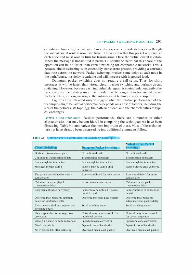
other characteristics Besides performance, there are a number of other characteristics that may be considered in comparing the techniques we have been discussing. Table 9.1 summarizes the most important of these. Most of these charac-teristics have already been discussed. A few additional comments follow.

Table 9.1 Comparison of Communication Switching Techniques

Circuit Switching Datagram Packet SwitchingVirtual Circuit Packet Switching

Dedicated transmission path No dedicated path No dedicated path

Continuous transmission of data Transmission of packets Transmission of packets

Fast enough for interactive Fast enough for interactive Fast enough for interactive

Messages are not stored Packets may be stored until delivered

Packets stored until delivered

The path is established for entire conversation

Route established for each packet Route established for entire conversation

Call setup delay; negligible transmission delay

Packet transmission delay Call setup delay; packet transmission delay

Busy signal if called party busy Sender may be notified if packet not delivered

Sender notified of connection denial

Overload may block call setup; no delay for established calls

Overload increases packet delay Overload may block call setup; increases packet delay

Electromechanical or computerized switching nodes

Small switching nodes Small switching nodes

User responsible for message loss protection

Network may be responsible for individual packets

Network may be responsible for packet sequences

Usually no speed or code conversion Speed and code conversion Speed and code conversion

Fixed bandwidth Dynamic use of bandwidth Dynamic use of bandwidth

No overhead bits after call setup Overhead bits in each packet Overhead bits in each packet


As was mentioned, circuit switching is essentially a transparent service. Once a connection is established, a constant data rate is provided to the connected stations. This is not the case with packet switching, which typically introduces variable delay, so that data arrive in a choppy manner. Indeed, with datagram packet switching, data may arrive in a different order than they were transmitted.

An additional consequence of transparency is that there is no overhead required to accommodate circuit switching. Once a connection is established, the analog or digital data are passed through, as is, from source to destination. For packet switching, analog data must be converted to digital before transmission; in addition, each packet includes overhead bits, such as the destination address.

9.6 asynchrOnOus transfer mOde

Asynchronous transfer mode is a switching and multiplexing technology that employs small, fixed-length packets called cells. A fixed-size packet was chosen to ensure that the switching and multiplexing function could be carried out effi-ciently, with little delay variation. A small cell size was chosen primarily to support delay-intolerant interactive voice service with a small packetization delay. ATM is a connection-oriented packet-switching technology that was designed to provide the performance of a circuit-switching network and the flexibility and efficiency of a packet-switching network. A major thrust of the ATM standardization effort was to provide a powerful set of tools for supporting a rich QoS capability and a powerful traffic management capability. ATM was intended to provide a unified networking standard for both circuit-switched and packet-switched traffic, and to support data, voice, and video with appropriate QoS mechanisms. With ATM, the user can select the desired level of service and obtain guaranteed service quality. Internally, the ATM network makes reservations and preplans routes so that transmission alloca-tion is based on priority and QoS characteristics.

ATM was intended to be a universal networking technology, with much of the switching and routing capability implemented in hardware, and with the ability to support IP-based networks and circuit-switched networks. It was also anticipated that ATM would be used to implement local area networks. ATM never achieved this comprehensive deployment. However, ATM remains an important technology. ATM is commonly used by telecommunications providers to implement wide area networks. Many DSL implementations use ATM over the basic DSL hardware for multiplexing and switching, and ATM is used as a backbone network technology in numerous IP networks and portions of the Internet.

A number of factors have led to this lesser role for ATM. IP, with its many associated protocols, provides an integrative technology that is more scalable and less complex than ATM. In addition, the need to use small fixed-sized cells to reduce jitter has disappeared as transport speeds have increased. The develop-ment of voice and video over IP protocols has provided an integration capability at the IP level.

Perhaps the most significant development related to the reduced role for ATM is the widespread acceptance of Multiprotocol Label Switching (MPLS). MPLS is

tipo de servicioa la carta.

ADSLModem.

Complicadoemular IP

9.6 / asynchronous Transfer mode 293

a layer-2 connection-oriented packet-switching protocol that, as the name suggests, can provide a switching service for a variety of protocols and applications, including IP, voice, and video. We introduce MPLS in Chapter 23.

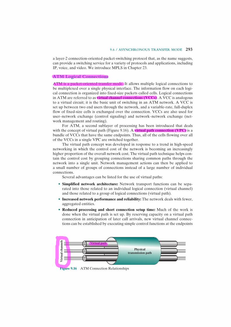
ATM Logical Connections

ATM is a packet-oriented transfer mode. It allows multiple logical connections to be multiplexed over a single physical interface. The information flow on each logi-cal connection is organized into fixed-size packets called cells. Logical connections in ATM are referred to as virtual channel connections (VCCs). A VCC is analogous to a virtual circuit; it is the basic unit of switching in an ATM network. A VCC is set up between two end users through the network, and a variable-rate, full-duplex flow of fixed-size cells is exchanged over the connection. VCCs are also used for user–network exchange (control signaling) and network–network exchange (net-work management and routing).

For ATM, a second sublayer of processing has been introduced that deals with the concept of virtual path (Figure 9.16). A virtual path connection (VPC) is a bundle of VCCs that have the same endpoints. Thus, all of the cells flowing over all of the VCCs in a single VPC are switched together.

The virtual path concept was developed in response to a trend in high-speed networking in which the control cost of the network is becoming an increasingly higher proportion of the overall network cost. The virtual path technique helps con-tain the control cost by grouping connections sharing common paths through the network into a single unit. Network management actions can then be applied to a small number of groups of connections instead of a large number of individual connections.

Several advantages can be listed for the use of virtual paths:

• Simplified network architecture: Network transport functions can be sepa-rated into those related to an individual logical connection (virtual channel) and those related to a group of logical connections (virtual path).

• Increased network performance and reliability: The network deals with fewer, aggregated entities.

• Reduced processing and short connection setup time: Much of the work is done when the virtual path is set up. By reserving capacity on a virtual path connection in anticipation of later call arrivals, new virtual channel connec-tions can be established by executing simple control functions at the endpoints

Physicaltransmission path

Virtual path

Vir

tual

cha

nnel

s

Figure 9.16 ATM Connection Relationships


of the virtual path connection; no call processing is required at transit nodes. Thus, the addition of new virtual channels to an existing virtual path involves minimal processing.

• Enhanced network services: The virtual path is used internal to the network but is also visible to the end user. Thus, the user may define closed user groups or closed networks of virtual channel bundles.

Virtual Path/Virtual channel characteristics ITU-T Recommendation I.150 lists the following as characteristics of virtual channel connections:

• Quality of service (QoS): A user of a VCC is provided with a QoS specified by parameters such as cell loss ratio (ratio of cells lost to cells transmitted) and cell delay variation.

• Switched and semipermanent virtual channel connections: A switched VCC is an on-demand connection, which requires a call control signaling for setup and tearing down. A semipermanent VCC is one that is of long duration and is set up by configuration or network management action.

• Cell sequence integrity: The sequence of transmitted cells within a VCC is preserved.

• Traffic parameter negotiation and usage monitoring: Traffic parameters can be negotiated between a user and the network for each VCC. The network monitors the input of cells to the VCC to ensure that the negotiated param-eters are not violated.

The types of traffic parameters that can be negotiated include average rate, peak rate, burstiness, and peak duration. The network may need a number of strat-egies to deal with congestion and to manage existing and requested VCCs. At the crudest level, the network may simply deny new requests for VCCs to prevent con-gestion. Additionally, cells may be discarded if negotiated parameters are violated or if congestion becomes severe. In an extreme situation, existing connections might be terminated.

I.150 also lists characteristics of VPCs. The first four characteristics listed are identical to those for VCCs. That is, QoS; switched and semipermanent VPCs; cell sequence integrity; and traffic parameter negotiation and usage monitoring are all also characteristics of a VPC. There are a number of reasons for this duplica-tion. First, this provides some flexibility in how the network service manages the requirements placed upon it. Second, the network must be concerned with the overall requirements for a VPC, and within a VPC may negotiate the establishment of virtual channels with given characteristics. Finally, once a VPC is set up, it is possible for the end users to negotiate the creation of new VCCs. The VPC charac-teristics impose a discipline on the choices that the end users may make.

In addition, a fifth characteristic is listed for VPCs:

• Virtual channel identifier restriction within a VPC: One or more virtual chan-nel identifiers, or numbers, may not be available to the user of the VPC but may be reserved for network use. Examples include VCCs used for network management.

9.6 / asynchronous Transfer mode 295

control signaling In ATM, a mechanism is needed for the establishment and release of VPCs and VCCs. The exchange of information involved in this process is referred to as control signaling and takes place on separate connections from those that are being managed.

For VCCs, I.150 specifies four methods for providing an establishment/release facility. One or a combination of these methods will be used in any particular network:

1. Semipermanent VCCs may be used for user-to-user exchange. In this case, no control signaling is required.

2. If there is no preestablished call control signaling channel, then one must be set up. For that purpose, a control signaling exchange must take place between the user and the network on some channel. Hence we need a perma-nent channel, probably of low data rate, that can be used to set up VCCs that can be used for call control. Such a channel is called a meta-signaling channel, as the channel is used to set up signaling channels.

3. The meta-signaling channel can be used to set up a VCC between the user and the network for call control signaling. This user-to-network signaling virtual channel can then be used to set up VCCs to carry user data.

4. The meta-signaling channel can also be used to set up a user-to-user signaling virtual channel. Such a channel must be set up within a preestablished VPC. It can then be used to allow the two end users, without network intervention, to establish and release user-to-user VCCs to carry user data.

For VPCs, three methods are defined in I.150:

1. A VPC can be established on a semipermanent basis by prior agreement. In this case, no control signaling is required.

2. VPC establishment/release may be customer controlled. In this case, the customer uses a signaling VCC to request the VPC from the network.

3. VPC establishment/release may be network controlled. In this case, the network establishes a VPC for its own convenience. The path may be net-work-to-network, user-to-network, or user-to-user.

ATM Cells

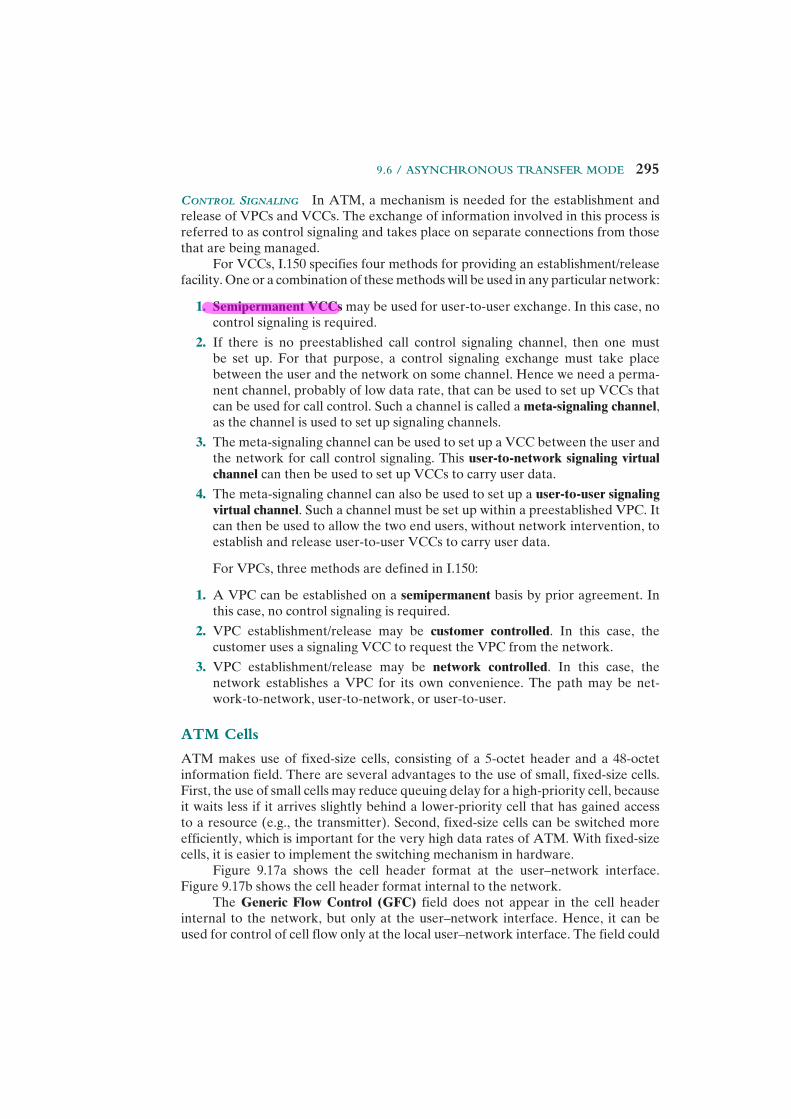
ATM makes use of fixed-size cells, consisting of a 5-octet header and a 48-octet information field. There are several advantages to the use of small, fixed-size cells. First, the use of small cells may reduce queuing delay for a high-priority cell, because it waits less if it arrives slightly behind a lower-priority cell that has gained access to a resource (e.g., the transmitter). Second, fixed-size cells can be switched more efficiently, which is important for the very high data rates of ATM. With fixed-size cells, it is easier to implement the switching mechanism in hardware.

Figure 9.17a shows the cell header format at the user–network interface. Figure 9.17b shows the cell header format internal to the network.

The Generic Flow Control (GFC) field does not appear in the cell header internal to the network, but only at the user–network interface. Hence, it can be used for control of cell flow only at the local user–network interface. The field could


be used to assist the customer in controlling the flow of traffic for different qualities of service. In any case, the GFC mechanism is used to alleviate short-term overload conditions in the network.

The virtual path identifier (VPI) constitutes a routing field for the network. It is 8 bits at the user–network interface and 12 bits at the network–network inter-face. The latter allows support for an expanded number of VPCs internal to the network, to include those supporting subscribers and those required for network management. The virtual channel identifier (VCI) is used for routing to and from the end user.

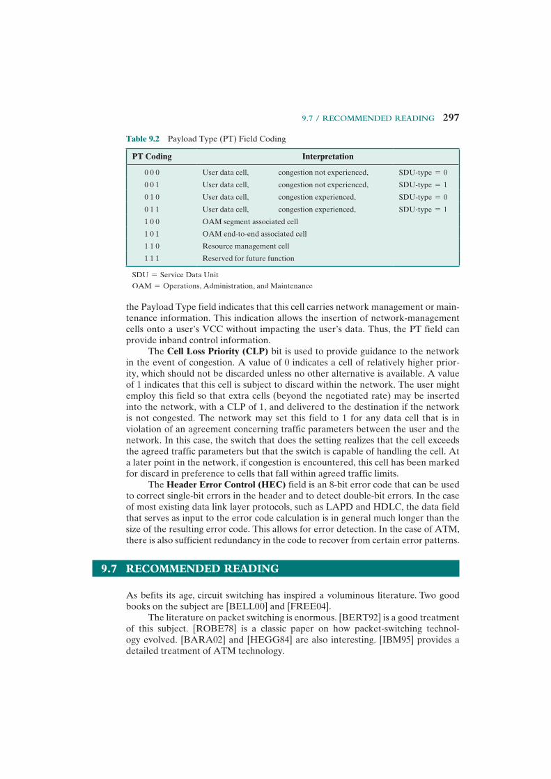
The Payload Type (PT) field indicates the type of information in the informa-tion field. Table 9.2 shows the interpretation of the PT bits. A value of 0 in the first bit indicates user information (i.e., information from the next higher layer). In this case, the second bit indicates whether congestion has been experienced; the third bit, known as the Service Data Unit (SDU) type bit, is a one-bit field that can be used to discriminate two types of ATM SDUs associated with a connection. The term SDU refers to the 48-octet payload of the cell. A value of 1 in the first bit of

Generic flow control Virtual path identifier

Virtual path identifier

Virtual channel identifier

Payload type CLP

Header error control

(a) User–network interface

Information field(48 octets)

(b) Network–network interface

Virtual path identifier

Virtual channel identifier

Header error control

Information field(48 octets)

8 7 6 5 4 3 2 1 8 7 6 5 4 3 2 1

Payload type CLP

5-octetheader

53-octetcell

Figure 9.17 ATM Cell Format

9.7 / recommended reading 297

the Payload Type field indicates that this cell carries network management or main-tenance information. This indication allows the insertion of network-management cells onto a user’s VCC without impacting the user’s data. Thus, the PT field can provide inband control information.

The Cell loss Priority (ClP) bit is used to provide guidance to the network in the event of congestion. A value of 0 indicates a cell of relatively higher prior-ity, which should not be discarded unless no other alternative is available. A value of 1 indicates that this cell is subject to discard within the network. The user might employ this field so that extra cells (beyond the negotiated rate) may be inserted into the network, with a CLP of 1, and delivered to the destination if the network is not congested. The network may set this field to 1 for any data cell that is in violation of an agreement concerning traffic parameters between the user and the network. In this case, the switch that does the setting realizes that the cell exceeds the agreed traffic parameters but that the switch is capable of handling the cell. At a later point in the network, if congestion is encountered, this cell has been marked for discard in preference to cells that fall within agreed traffic limits.

The Header Error Control (HEC) field is an 8-bit error code that can be used to correct single-bit errors in the header and to detect double-bit errors. In the case of most existing data link layer protocols, such as LAPD and HDLC, the data field that serves as input to the error code calculation is in general much longer than the size of the resulting error code. This allows for error detection. In the case of ATM, there is also sufficient redundancy in the code to recover from certain error patterns.

9.7 recOmmended reading

As befits its age, circuit switching has inspired a voluminous literature. Two good books on the subject are [BELL00] and [FREE04].

The literature on packet switching is enormous. [BERT92] is a good treatment of this subject. [ROBE78] is a classic paper on how packet-switching technol-ogy evolved. [BARA02] and [HEGG84] are also interesting. [IBM95] provides a detailed treatment of ATM technology.

Table 9.2 Payload Type (PT) Field Coding

PT Coding Interpretation

0 0 0 User data cell, congestion not experienced, SDU@type = 0

0 0 1 User data cell, congestion not experienced, SDU@type = 1

0 1 0 User data cell, congestion experienced, SDU@type = 0

0 1 1 User data cell, congestion experienced, SDU@type = 1

1 0 0 OAM segment associated cell

1 0 1 OAM end-to-end associated cell

1 1 0 Resource management cell

1 1 1 Reserved for future function

SDU = Service Data Unit

OAM = Operations, Administration, and Maintenance


9.8 key terms, review QuestiOns, and prObLems

Key Terms

asynchronous transfer mode (ATM)

cellcircuit switchingcircuit-switching networkcrossbar matrixdatagramdigital switchexchangeexternal virtual circuitgeneric flow control (GFC)

header error control (HEC)internal virtual circuitlocal loopmedia gateway controller

(MGC)packet switchingsoftswitchspace division switchingsubscribersubscriber linesubscriber loop

time-division switchingtime-multiplexed switching

(TMS)time-slot interchange (TSI)trunkvirtual channel connection

(VCC)virtual circuitvirtual path connection

(VPC)

Review Questions

9.1 Why is it useful to have more than one possible path through a network for each pair of stations?

9.2 What are the four generic architectural components of a public communications network? Define each term.

9.3 What is the principal application that has driven the design of circuit-switching networks?

9.4 What are the advantages of packet switching compared to circuit switching? 9.5 Explain the difference between datagram and virtual circuit operation. 9.6 What is the significance of packet size in a packet-switching network? 9.7 What types of delay are significant in assessing the performance of a packet-switching

network?

BARA02 Baran, P. “The Beginnings of Packet Switching: Some Underlying Concepts.” IEEE Communications Magazine, July 2002.

BEll00 Bellamy, J. Digital Telephony. New York: Wiley, 2000.BERT92 Bertsekas, D., and Gallager, R. Data Networks. Englewood Cliffs, NJ: Prentice

Hall, 1992.FREE04 Freeman, R. Telecommunication System Engineering. New York: Wiley, 2004.HEGG84 Heggestad, H. “An Overview of Packet Switching Communications.” IEEE

Communications Magazine, April 1984.IBM95 IBM International Technical Support Organization. Asynchronous Transfer

Mode (ATM) Technical Overview. IBM Redbook SG24-4625-00, 1995. www.red-books.ibm.com

ROBE78 Roberts, L. “The Evolution of Packet Switching.” Proceedings of the IEEE, November 1978.

[BERT92] is a good treatment of this subject.

9.8 / key Terms, revieW QuesTions, and Problems 299

9.8 What are the characteristics of a virtual channel connection? 9.9 What are the characteristics of a virtual path connection? 9.10 List and briefly explain the fields in an ATM cell.

Problems

9.1 Consider a simple telephone network consisting of two end offices and one inter-mediate switch with a 1-MHz full-duplex trunk between each end office and the intermediate switch. Assume a 4-kHz channel for each voice call. The average tele-phone is used to make four calls per 8-hour workday, with a mean call duration of six minutes. Ten percent of the calls are long distance. What is the maximum number of telephones an end office can support?

9.2 a. If a crossbar matrix has n input lines and m output lines, how many crosspoints are required?

b. How many crosspoints would be required if there were no distinction between input and output lines (i.e., if any line could be interconnected to any other line serviced by the crossbar)?

c. Show the minimum configuration. 9.3 Consider a three-stage switch such as in Figure 9.6. Assume that there are a total of N

input lines and N output lines for the overall three-stage switch. If n is the number of input lines to a stage 1 crossbar and the number of output lines to a stage 3 crossbar, then there are N/n stage 1 crossbars and N/n stage 3 crossbars. Assume each stage 1 crossbar has one output line going to each stage 2 crossbar, and each stage 2 crossbar has one output line going to each stage 3 crossbar. For such a configuration it can be shown that, for the switch to be nonblocking, the number of stage 2 crossbar matrices must equal 2n − 1.

a. What is the total number of crosspoints among all the crossbar switches? b. For a given value of N, the total number of crosspoints depends on the value of

n. That is, the value depends on how many crossbars are used in the first stage to handle the total number of input lines. Assuming a large number of input lines to each crossbar (large value of n), what is the minimum number of crosspoints for a nonblocking configuration as a function of n?

c. For a range of N from 102 to 106, plot the number of crosspoints for a single-stage N * N switch and an optimum three-stage crossbar switch.

9.4 Consider a TSI system with a TDM input of 8000 frames per second. The TSI requires one memory read and one memory write operation per slot. What is the maximum number of slots per frame that can be handled, as a function of the memory cycle time?

9.5 Consider a TDM system with 8 I/O lines, and connections 1-2, 3-7, and 5-8. Draw several frames of the input to the TSI unit and output from the TSI unit, indicating the movement of data from input time slots to output time slots.

9.6 Explain the flaw in the following reasoning: Packet switching requires control and address bits to be added to each packet. This introduces considerable overhead in packet switching. In circuit switching, a transparent circuit is established. No extra bits are needed. Therefore, there is no overhead in circuit switching. Because there is no overhead in circuit switching, line utilization must be more efficient than in packet switching.

9.7 Define the following parameters for a switching network:

N = number of hops between two given end systemsL = message length in bitsB = data rate, in bits per second (bps), on all linksP = fixed packet size, in bits


H = overhead (header) bits per packetS = call setup time (circuit switching or virtual circuit) in seconds

D = propagation delay per hop in seconds

a. For N = 4, L = 3200, B = 9600, P = 1024, H = 16, S = 0.2, D = 0.001, compute the end-to-end delay for circuit switching, virtual circuit packet switching, and datagram packet switching. Assume that there are no acknowledgments. Ignore processing delay at the nodes.

b. Derive general expressions for the three techniques of part (a), taken two at a time (three expressions in all), showing the conditions under which the delays are equal.

9.8 What value of P, as a function of N, L, and H, results in minimum end-to-end delay on a datagram network? Assume that L is much larger than P, and D is zero.

9.9 Assuming no malfunction in any of the stations or nodes of a network, is it possible for a packet to be delivered to the wrong destination?

9.10 Although ATM does not include any end-to-end error detection and control func-tions on the user data, it is provided with a HEC field to detect and correct header errors. Let us consider the value of this feature. Suppose that the bit error rate of the transmission system is B. If errors are uniformly distributed, then the probability of an error in the header is

hh + i

* B

and the probability of error in the data field is

ih + i

* B

where h is the number of bits in the header and i is the number of bits in the data field. a. Suppose that errors in the header are not detected and not corrected. In that case,

a header error may result in a misrouting of the cell to the wrong destination; therefore, i bits will arrive at an incorrect destination, and i bits will not arrive at the correct destination. What is the overall bit error rate B1? Find an expression for the multiplication effect on the bit error rate: M1 = B1>B.

b. Now suppose that header errors are detected but not corrected. In that case, i bits will not arrive at the correct destination. What is the overall bit error rate B2? Find an expression for the multiplication effect on the bit error rate: M2 = B2>B.

c. Now suppose that header errors are detected and corrected. What is the overall bit error rate B3? Find an expression for the multiplication effect on the bit error rate: M3 = B3>B.

d. Plot M1, M2, and M3 as a function of header length, for i = 48 * 8 = 384 bits. Comment on the results.

9.11 One key design decision for ATM was whether to use fixed- or variable-length cells. Let us consider this decision from the point of view of efficiency. We can define trans-mission efficiency as

N =Number of information octets

Number of information octets + Number of overhead octets

a. Consider the use of fixed-length packets. In this case the overhead consists of the header octets. Define

L = Data field size of the cell in octets H = Header size of the cell in octets X = Number of information octets to be transmitted as a single message

9.8 / key Terms, revieW QuesTions, and Problems 301

Derive an expression for N. Hint: The expression will need to use the operator < ~ =, where <Y= = the smallest integer greater than or equal to Y. b. If cells have variable length, then overhead is determined by the header, plus

the flags to delimit the cells or an additional length field in the header. Let Hv = additional overhead octets required to enable the use of variable-length cells. Derive an expression for N in terms of X, H, and Hv.

c. Let L = 48, H = 5, and Hv = 2. Plot N versus message size for fixed- and vari-able-length cells. Comment on the results.

9.12 Another key design decision for ATM is the size of the data field for fixed-size cells. Let us consider this decision from the point of view of efficiency and delay.a. Assume that an extended transmission takes place, so that all cells are completely

filled. Derive an expression for the efficiency N as a function of H and L.b. Packetization delay is the delay introduced into a transmission stream by the need

to buffer bits until an entire packet is filled before transmission. Derive an expres-sion for this delay as a function of L and the data rate R of the source.

c. Common data rates for voice coding are 32 kbps and 64 kbps. Plot packetiza-tion delay as a function of L for these two data rates; use a left-hand y axis with a maximum value of 2 ms. On the same graph, plot transmission efficiency as a function of L; use a right-hand y-axis with a maximum value of 100%. Comment on the results.

9.13 Consider compressed video transmission in an ATM network. Suppose standard ATM cells must be transmitted through 5 switches. The data rate is 43 Mbps.a. What is the transmission time for one cell through one switch?b. Each switch may be transmitting a cell from other traffic all of which we assume

to have lower (non-preemptive for the cell) priority. If the switch is busy trans-mitting a cell, our cell has to wait until the other cell completes transmission. If the switch is free our cell is transmitted immediately. What is the maximum time when a typical video cell arrives at the first switch (and possibly waits) until it is finished being transmitted by the fifth and last one? Assume that you can ignore propagation time, switching time, and everything else but the transmission time and the time spent waiting for another cell to clear a switch.

c. Now suppose we know that each switch is utilized 60% of the time with the other low-priority traffic. By this we mean that with probability 0.6 when we look at a switch it is busy. Suppose that if there is a cell being transmitted by a switch, the average delay spent waiting for a cell to finish transmission is one-half a cell transmission time. What is the average time from the input of the first switch to clearing the fifth?

d. However, the measure of most interest is not delay but jitter, which is the vari-ability in the delay. Use parts (b) and (c) to calculate the maximum and average variability, respectively, in the delay.

In all cases assume that the various random events are independent of one another; for example, we ignore the burstiness typical of such traffic.

9.14 In order to support IP service over an ATM network, IP datagrams must first be seg-mented into a number of ATM cells before sending them over the ATM network. As ATM does not provide cell loss recovery, the loss of any of these cells will result in the loss of the entire IP packet. Given:

PC = cell loss rate in the ATM network n = number of cells required to transmit a single IP datagram

PP = IP@packet loss rate

a. Derive an expression for PP, and comment on the resulting expression. b. What ATM service would you use to get the best possible performance?

9.5 packet-switching principles - aula virtual

Documents