2018mcconville10173913.pdf - university of plymouth pearl
TRANSCRIPT
University of Plymouth
PEARL https://pearl.plymouth.ac.uk
04 University of Plymouth Research Theses 01 Research Theses Main Collection
2018
Trophic and ecological implications of
the gelatinous body form in zooplankton
McConville, Kristian
http://hdl.handle.net/10026.1/11835
University of Plymouth
All content in PEARL is protected by copyright law. Author manuscripts are made available in accordance with
publisher policies. Please cite only the published version using the details provided on the item record or
document. In the absence of an open licence (e.g. Creative Commons), permissions for further reuse of content
should be sought from the publisher or author.
i
This copy of the thesis has been supplied on condition that anyone who consults it is understood torecognise that its copyright rests with its author and that no quotation from the thesis and no
information derived from it may be published without the author's prior consent.
ii
TROPHIC AND ECOLOGICAL IMPLICATIONS OF THE GELATINOUS BODY FORM INZOOPLANKTON
By
KRISTIAN M. McCONVILLE
A thesis submitted to the University of Plymouth
in partial fulfilment for the degree of
DOCTOR OF PHILOSOPHY
School of Biological & Marine Sciences
[In collaboration with Plymouth Marine Laboratory]
June 2018
iii
Trophic and ecological implications of the gelatinous body form in zooplankton
Kristian Michael McConville
Gelatinous zooplankton are characterised as different from other planktonic taxa due to the highrelative water content of their tissues. This thesis investigates whether elevated somatic watercontent (expressed here as carbon percentage) has effects on the biology of zooplankton. Myapproach was to examine this at a range of scales with a variety of approaches, ranging fromexperiments on individual ephyra larvae of Aurelia aurita, through analysis of a zooplankton timeseries at the Plymouth L4 station, up to a large scale meta-analysis of zooplankton growth andbody composition data. In this meta-analysis, carbon percentage varied continuously across therange of the zooplankton, ranging from 0.01% to 19.02% of wet mass, a difference of over threeorders of magnitude. Specific growth rate (g, d-1) was negatively related to carbon percentage,both across the full range of zooplankton species, and within the subset of taxa traditionallyclassified as gelatinous. The addition of carbon percentage to models of zooplankton growth ratebased on carbon mass alone doubled explanatory power. I present an empirical equation ofmaximum (food saturated) zooplankton growth that incorporates carbon mass and carbon as apercentage of wet mass. Applying this equation to a natural assemblage near Plymouth yieldedsometimes double the secondary production, as compared to a simpler model based oncrustacean growth. Both interspecifically and intraspecifically, carbon percentage was negativelyrelated to carbon mass; more gelatinous taxa tended to have higher carbon masses. During theearly development of Aurelia aurita ephyrae, carbon percentage was found to decrease from2.36% (an intermediate value between crustaceans and classical gelatinous zooplankton) down to0.1%, the adult value for Aurelia aurita. Juvenile forms of gelatinous taxa are often poorly sampledand their intermediate carbon percentages may help to form a continuum between those ofcrustaceans and adult cnidarians and ctenophores. As ingestion in the ephyrae was related to theirdiameter, models suggest that this dilution resulted in an increase in carbon-specific ingestion rateby an estimated 28% relative to an ephyra that did not dilute through development. At the specieslevel, carbon percentage was negatively related to indices of temporal variation in numericaldensity but not related to rate of population increase. A wide variety of zooplanktonic taxa ofdifferent carbon percentages were found to increase in population at a rate that could beconsidered as forming a bloom. Likewise many gelatinous taxa at L4 did not form blooms. Thus thefrequent reference to “jellyfish blooms” reflects, in part, the fact that unlike the other zooplanktersthat regularly reach even higher carbon concentrations, gelatinous taxa are simply more noticeableto the eye when at these concentrations. Calculating the carbon percentage of whole assemblagescould be useful for investigating the influence of environmental parameters on zooplankton. Takentogether, these results demonstrate the benefits of explicitly recognising the decoupling ofmetabolic and ecological body size seen in the gelatinous zooplankton.

iv
Contents
Abstract……………………………………………………………………………………………………….iii
Contents………………………………………………………………………………………………………iv
Figure and Table Contents…………………………………………………………………………………vii
Acknowledgements…………………………………………………………………………………………..x
Author’s Declaration………………………………………………………………………………………...xi
CHAPTER 1 - Introduction..............................................................................................................................1
1.1 - Importance of gelatinous zooplankton.............................................................................................2
1.2 - Biological implications of a gelatinous body form.......................................................................... 6
1.3 - Aims and layout of this thesis............................................................................................................7
1.3.1 - Aim.................................................................................................................................................9
1.3.2 - Objectives..................................................................................................................................... 9
CHAPTER 2 – Theoretical model of the effects of carbon percentage and L4 sampling details......13
2.1 - Introduction........................................................................................................................................ 14
2.2 - Dilution as a continuous trait: modelling the potential effects of carbon percentage.............14
2.2.1 - Respiration..................................................................................................................................15
2.2.2 - Ingestion rate..............................................................................................................................15
2.2.3 - Scope for growth........................................................................................................................17
2.3 - Introduction to the Western Channel Observatory...................................................................... 17
2.3.1 - L4 zooplankton time series sampling.....................................................................................19
CHAPTER 3 – Disentangling the counteracting effects of water content and carbon mass onzooplankton growth........................................................................................................................................21
3.1 - Introduction........................................................................................................................................ 22
3.2 - Methods..............................................................................................................................................23
3.2.1 - Carbon percentage data...........................................................................................................23
3.2.2 – Analysis of the zooplankton assemblage from the L4 site.................................................24
3.2.3 - Growth rate data........................................................................................................................24
3.2.4 - Growth rate analysis................................................................................................................. 25
3.2.5 – Secondary production..............................................................................................................26
3.3 - Results................................................................................................................................................26
3.3.1 - Variability in carbon percentage across the zooplankton....................................................26
3.3.2 - Relationship between carbon mass and carbon percentage............................................. 33
3.3.3 - Relationship between carbon percentage and growth rate................................................ 34
3.3.4 – Secondary production..................................................................................................................38
v
3.5 - Discussion..........................................................................................................................................40
3.6 - Conclusions....................................................................................................................................... 44
CHAPTER 4 – Intraspecific effects of variable carbon percentage through ontogeneticdevelopment: morphometrics, feeding and growth of Aurelia aurita ephyrae......................................47
4.1 - Introduction........................................................................................................................................ 48
4.2 - Methods..............................................................................................................................................50
4.2.1 - Experiment and measurement................................................................................................ 50
4.2.2 - Numerical methods................................................................................................................... 53
4.3 – Results...............................................................................................................................................54
4.3.1 - Morphometrics........................................................................................................................... 54
4.3.2 – Ingestion rate.............................................................................................................................56
4.3.3 - Growth rate.................................................................................................................................57
4.3.3 - Implications of changing carbon percentage for ingestion and growth rates...................59
4.4 - Discussion..........................................................................................................................................63
4.4.1 - Ingestion......................................................................................................................................65
4.4.2 - Growth.........................................................................................................................................67
4.5 - Conclusion......................................................................................................................................... 68
CHAPTER 5 – The influence of carbon percentage on bloom formation.............................................71
5.1 - Introduction........................................................................................................................................ 72
5.2 - Methods..............................................................................................................................................75
5.2.1 - Data sources.............................................................................................................................. 75
5.2.2 - Development of bloom indices................................................................................................ 75
5.2.3 - Variability in abundance........................................................................................................... 76
5.2.4 - Temporal heterogeneity............................................................................................................77
5.2.5 - Population increase rate...........................................................................................................79
5.2.6 - Testing bloom index performance.......................................................................................... 80
5.3 - Results................................................................................................................................................82
5.3.1 – Variability....................................................................................................................................87
5.3.1.1 – Testing of variability indices.................................................................................................87
5.3.1.2 – Effect of carbon percentage on variability indices............................................................87
5.3.2 - Temporal heterogeneity............................................................................................................88
5.3.2.1 – Testing of temporal heterogeneity indices........................................................................ 88
5.3.2.2 – Effect of carbon percentage on temporal heterogeneity indices................................... 88
5.3.3 - Population increase rate...........................................................................................................88
5.3.3.1 – Testing of population increase rate indices.......................................................................88
5.3.3.2 – Effect of carbon percentage on population increase rate indices..................................89
5.4 – Discussion.........................................................................................................................................89
vi
5.4.1 – Variability in abundance.......................................................................................................... 89
5.4.1.1 – Are the variability-based bloom indices effective?...........................................................89
5.4.1.2 – The relationship between carbon percentage and variability in abundance................90
5.4.2 - Temporal heterogeneity............................................................................................................91
5.4.2.1 – Are the temporal heterogeneity based bloom indices effective?...................................91
5.4.2.2 – Discussing the relationship between carbon percentage and temporal heterogeneity91
5.4.3 - Population increase rate...........................................................................................................92
5.4.3.1 – Are the population increase based bloom indices effective?.........................................92
5.4.3.2 – Discussing the relationship between carbon percentage and increase rate............... 93
5.4.4 – Are taxa with higher carbon percentages also blooming?.................................................93
CHAPTER 6 – Body size as a function of carbon mass and carbon percentage............................. 101
6.1 - Introduction......................................................................................................................................102
6.2 - What is the relationship between carbon percentage and carbon mass, and why is itimportant?.................................................................................................................................................103
6.3 - Carbon percentage – carbon mass trait space..........................................................................104
6.3.1 - Area a: high carbon mass and high carbon percentage...................................................106
6.3.2 - Area b: high carbon mass and low carbon percentage.....................................................107
6.3.3 - Area c: low carbon mass and low carbon percentage...................................................... 108
6.4 - Pseudo gelatinous taxa................................................................................................................. 108
6.5 - Carbon mass and carbon percentage at the L4 study site...................................................... 110
6.6 - Conclusion.......................................................................................................................................113
CHAPTER 7 – Concluding discussion..................................................................................................... 116
7.1 - Introduction......................................................................................................................................117
7.2 - Carbon percentage as a predictor variable for biological rates...............................................117
7.2.1 - Feeding rates...........................................................................................................................118
7.2.2 - Growth rates.............................................................................................................................119
7.3 - Population dynamics......................................................................................................................120
7.4 - Addition of carbon percentage to trait based models............................................................... 121
7.5 - Carbon percentage as an ecological indicator...........................................................................122
7.6 - Closing remarks..............................................................................................................................126
References....................................................................................................................................................128
Appendix I – Carbon percentage.............................................................................................................. 150
Appendix II – Growth rates.........................................................................................................................155
Appendix III – L4 measurements and indices.........................................................................................213
Appendix IV – Published work...................................................................................................................223
vii
Figure Contents
Figure 1.1 – Number of peer reviewed articles per year returned from a Web of Science search(accessed 26/01/17) with the following criteria: (“jellyfish” OR “gelatinous”) AND “bloom*” on theprimary y axis (shown in red) and “zooplankton” on the secondary y axis (shown in green)................
Figure 2.1 – Location of the sampling stations within the Western Channel Observatory offPlymouth, UK (http://www.westernchannelobservatory.org.uk).................................................................
Figure 3.1 - Comparison of the relative carbon (black) and wet masses (grey) of Calanushyperboreus (left, carbon percentage = 19.02%) and Bathycyroe fosteri (right, carbon percentage =0.01%). The relative area of each shade is scaled as volume so the silhouettes are representativeof true size...........................................................................................................................................................
Figure 3.2 - (a) Zooplankton species ranked according to their carbon percentage (CM%WM; log10scale), each horizontal bar represents a single species. Colours indicate taxonomic groups asdetailed in the legend. (b) Zooplankton taxonomic groups ranked according to their carbon mass(as % of wet mass; log10 scale). Boxes indicate median, lower and upper quartiles with whiskersshowing the range. (Vertical lines at 0.5 and 5 CM%WM represent the composition of thegelatinous and non-gelatinous taxa defined by Kiørboe, 2013).................................................................
Figure 3.3 - Distribution of carbon biomass (mg C m-3) between log2 carbon percentage categoriesthrough spring, summer, autumn and winter (2009-2015) at the L4 sampling site, Western ChannelObservatory, Plymouth. The same colour coding of taxa is used as in Figure 3.1 – see legend. * -Biomass value for the category 0.4 – 0.8 exceeds the scale in summer (crudely estimated at 34 mgC m-3) as a result of 7 high abundance observations of Beroe spp. (of total 318 samples). Upperlimit of biomass scale in winter is 5 mg C m-3................................................................................................
Figure 3.4 – Log10 carbon percentage (CM%WM) as a function of log10 carbon mass (mg) for themeta-analysis dataset (log10 carbon percentage = - 0.17 * log10 carbon mass – 0.3, p = 0.0003, R2
= 0.12, df = 108). Taxonomic groups are coloured as indicated in the legends......................................
Figure 3.5 – Log10 specific growth rate, g (d-1) as a function of log10 carbon percentage (CM%WM).Growth values were temperature-adjusted to 15oC then mass adjusted to 1 mg C. (a) mean mass-specific growth rate values for each species in each study and (b) maximum specific growth ratevalues for each species.....................................................................................................................................
Figure 3.6 – Estimates of secondary production at the L4 sampling site at weekly resolutionbetween 05/01/2009 and 15/12/2012. Growth rates were estimated on the basis of carbon massalone (log carbon specific growth rate (mg C mg C-1 h-1) = - 2.82 - 0.31 log10 carbon mass(mg))using the equation for crustaceans from Kiørboe and Hirst (2014) and carbon mass alongsidecarbon percentage (log specific growth rate, g, ((d-1) - 0.81 - 0.16 log10 carbon mass (mg) - 0.16log10 carbon percentage ((CM/WM)*100) using the maximum growth rate equation for allzooplankton shown in Table 3.1. Growth rates were temperature adjusted using a Q10 of 2.8(Hansen et al., 1997). Secondary production for each species was estimated as the growth incarbon mass per individual, multiplied by abundance. Species secondary production was summedacross species at each time point to estimate total secondary production…………………………..39
Figure 4.1 – Photomicrograph of an Aurelia aurita ephyra; the inter-rhopalial diameter is indicatedby the white line superimposed on the image (IRD = 4.8mm)....................................................................
Figure 4.2 – Wet mass (mg) as a function of carbon mass (mg) in Aurelia aurita ephyrae. Axes areon a logarithmic scale (base 10), each point represents an individual ephyra (df = 190)......................
viii
Figure 4.3 – Carbon mass as a percentage of wet mass, as a function of diameter (mm) in Aureliaaurita ephyrae. Axes are on a logarithmic scale (base 10), each point represents an individualephyra (df = 190)................................................................................................................................................
Figure 4.4 – Nitrogen mass (mg) as a function of carbon mass (mg) in Aurelia aurita ephyrae. Eachpoint represents an individual ephyra (df = 190)...........................................................................................
Figure 4.5 – Ingestion rate (µg C ind-1 d-1) of Aurelia aurita ephyrae as a function of carbon mass(mg, log10y = 0.6 * log10x + 2.04, R2 = 0.58, p < 0.0001), wet mass (mg, log10y = 0.33 * log10x –2.07, R2 = 0.4, p < 0.0001) and carbon percentage (log10y = - 0.35 * log10x + 1.12, R2 = 0.07, p =0.047). Axes are on a logarithmic scale (base 10), each point represents an individual ephyra (df =41).........................................................................................................................................................................
Figure 4.6 – Ingestion rate (ug C ind-1 d-1) as a function of diameter (mm) in Aurelia aurita ephyrae,(df = 55)................................................................................................................................................................
Figure 4.7 – Growth rate as a function of mass in Aurelia aurita ephyrae. Axes are on a logarithmicscale (base 10), each point represents one replicate bottle (n=55); effect of carbon mass (mg) oncarbon mass growth rate (mg C h-1, A, log10y = 0.49 * log10x – 0.14, R2 = 0.2, p = 0.0028), carbonmass specific growth rate (mg C mg C h-1, B, log10y = - 0.51 * log10x – 0.14, R2 = 0.21, p = 0.0022),specific growth rate, g (d-1, C, log10y = - 0.36 * log10x – 1.54, R2 = 0.08, p = 0.04 ), effect of wetmass (mg) on wet mass growth rate (mg WM h-1, D, log10y = 0.62 * log10x - 1.07, R2 = 0.46, p <0.0001), wet mass specific growth rate (mg WM mg WM h-1, E, log10y = - 0.3 * log10x + 1.07, R2 =0.23, p = 0.0013), specific growth rate, g (d-1, F, log10y = - 0.34 * log10x – 0.53, R2 = 0.2, p = 0.0028)and effect of carbon percentage on carbon mass growth rate (mg C h-1, G, log10y = – 0.31* log10x -0.9, R2 = 0.01, p = 0.23), carbon mass specific growth rate (mg C mg C h-1, H, log10y = 0.59 *log10x + 0.7, R2 = 0.12, p = 0.02) and specific growth rate, g (d-1, I, log10y = 0.77 * log10x - 0.87, R2
= 0.21, p = 0.002)...............................................................................................................................................
Figure 4.8 – Effect of carbon mass (mg) on wet mass (mg) of Aurelia aurita ephyrae. Values aremodelled based on calculated carbon percentage across the range of diameters measured in thisstudy. In the gelatinous treatment, carbon percentage is allowed to vary following the relationshipshown in Figure 4.2, in the non-gelatinous treatment the carbon percentage is fixed at the startingvalue.....................................................................................................................................................................
Figure 4.9 – Effect of carbon mass (mg) on ingestion rate (mg C h-1) of Aurelia aurita ephyrae.Values are modelled based on the relationships between wet mass and ingestion rate shown inFigure 4.5. In the gelatinous treatment the carbon percentage is allowed to vary in the relationshipshown in Figure 4.2, in non-gelatinous the carbon percentage is fixed at the starting value................
Figure 4.10 – Growth in terms of daily change in wet mass (mg) of Aurelia aurita ephyrae. Valuesare modelled based on the relationships between wet mass and ingestion rate observed in ourdata. In the gelatinous treatment, carbon percentage is allowed to vary in the relationshipobserved in our data, in non-gelatinous the carbon percentage is fixed at the starting value...............
Figure 5.1 – Schematic data of abundance of two species over the year to demonstrate howblooming can be quantified on the basis of abundance over time. Note that while the schematicshows changes over monthly timescales, the sampling at L4 is on a weekly basis, weatherpermitting.............................................................................................................................................................
Figure 5.2 – Schematic example of the frequency distribution coefficient, the slope of a linearmodel between abundance (as % of maximum abundance) and log10 frequency. In the actualanalysis the x axis bins were of width 1% however this number of bins could not be clearly shown...
Figure 5.3 – Schematic example of the increase rate index, calculated for four increases as (n+4 -n) / 4. The points on the black line are data, the red line shows the range over which the increase
ix
rate for four successive increases is calculated. The green lines show two valid two step increasesacross four successive points...........................................................................................................................
Figure 5.4 – Abundance of Oithona similis (red) and Pleurobrachia pileus (blue) as a percentage ofthe total abundance of each species between 2009 and 2015...................................................................
Figure 5.5 – Relationships between carbon percentage, carbon mass and bloom indices forzooplankton taxa at the L4 sampling site. A - coefficient of variation in abundance of zooplankton atL4 as a function of log10 carbon percentage (df = 124, p = 0.013, adj R2 = 0.033, coefficient ofvariation = - 0.12 * log10 carbon percentage + 0.8), B – log10 interannual variability (maximumannual abundance / minimum annual abundance) as a function of log10 carbon percentage (df = 80,p = 0.07, adj R2 = 0.01, log10 interannual variability = - 5.06 * log10 carbon percentage + 68.3), C –log10 number of non-zero abundance records as a function of log10 carbon percentage (df = 124, p= 0.001, adj R2 = 0.07, number of non-zero records = 6.52 * carbon percentage – 58.1), D –coefficient of linear models between abundance and frequency as a function of log10 carbonpercentage (df = 77, p = 0.0005, adj R2 = 0.14, frequency distribution coefficient = 0.61 * carbonpercentage - 20.1), E – log10 maximum increase rate index across four successive increases as afunction of log10 carbon percentage (no statistically significant relationship detected), F – log10maximum increase rate index across four successive increases as a function of log10 carbon mass(df = 68, p = 0.0002, adj R2 = 0.16, log10 maximum increase rate index = - 0.46 * carbonpercentage + 1.62).............................................................................................................................................
Figure 5.6 – Three-point running mean abundance of Calanus helgolandicus and Pleurobrachiapileus at the L4 site between 05/01/2009 and 15/12/2015, normalised to the maximum abundancefor each species..................................................................................................................................................
Figure 5.7 - Three-point running mean abundance of Temora longicornis and Muggiaea atlantica atthe L4 site between 05/01/2009 and 15/12/2015, normalised to the maximum abundance for eachspecies.................................................................................................................................................................
Figure 5.8 – Ranked maximum recorded carbon biomasses (highest weekly value, mg C m-3) forzooplankton taxa at L4 between 2009 and 2015. This plot excludes Beroe spp., due tofragmentation and uncertainty over linear dimensions, precluding a robust biomass estimate............
Figure 5.9 – Ranked maximum recorded wet biomasses (highest weekly value, mg C m-3) forzooplankton taxa at L4 between 2009 and 2015..........................................................................................
Figure 5.10 – Two dimensional representation of one litre of sea water showing the volumeoccupied by a – Pleurobrachia pileus and b – Calanus helgolandicus during their respective wetbiomass maxima shown in Figure 5.8. Despite the greater visibility of the Pleurobrachia pileus, thecorresponding carbon mass of Calanus helgolandicus in panel b is six times greater than that ofPleurobrachia pileus in panel a........................................................................................................................
Figure 6.1 – Log10 carbon percentage of zooplankton ((carbon mass / wet mass)*100) as a functionof log10 carbon mass (mg) as compiled from literature sources (see Appendix I), df = 106, p =0.0003, R2 = 0.12, log10 carbon percentage = 0.30 – 0.1672 log10 carbon mass....................................
Figure 6.2 – Distribution of mean zooplankton biomass across axes of log10 carbon percentage andlog10 carbon (a) or log10 wet (b) mass at the L4 sampling site between 1988 and 2016. Biomass foreach species was averaged across all time points. Larger bubbles indicate higher mean taxonbiomass. Carbon masses were measured and carbon percentages were assigned as described inChapter 5.............................................................................................................................................................
Figure 7.1 – Monthly average assemblage carbon percentage at the L4 sampling site between1988 and 2016. Assemblage carbon percentage was calculated as the sum of abundance of eachtaxon multiplied by their carbon mass, divided by the sum of the abundance of each taxon
x
multiplied by their wet mass. Assemblage carbon percentage at each time point was sorted bymonth, and then averaged................................................................................................................................
Figure 7.2 – Assemblage carbon percentage (averaged by year) at the L4 sampling site recordedweekly between 1988 and 2016. Carbon percentages assigned as described in Chapter 4, df = 28,p = 0.0037, R2 = 0.26, carbon percentage = - 0.0615 year + 129.68. Ctenophores were omitteddue to potential preservation and recording issues......................................................................................
Figure 7.3 – Trends in assemblage carbon percentage at the L4 sampling site between 1988 and2016 in different seasons (winter = Jan, Feb, Mar, spring = Apr, May, Jun, summer = July, Aug,Sep, autumn = Oct, Nov, Dec). Spring carbon percentage = - 0.0457 year + 100.21, p = 0.052, R2
= 0.13. Summer carbon percentage = - 0.0615 year + 128.3, p = 0.104, R2 = 0.095. Autumn carbonpercentage = - 0.0971 year + 199.2, p = 0.007, R2 = 0.24. Winter carbon percentage = 0.0275 year+ 62.422, p = 0.33, R2 = 0.036. As above, ctenophores were omitted due to potential identificationand recording issues..........................................................................................................................................
Table Contents
Table 3.1 - General linear models predicting log10 mean specific and log10maximum specificgrowth rate, g (d-1), as a function of both log10 carbon mass (mg) and log10 body carbonpercentage (100*(CM/WM)). All models pertain to growth rate data that were first Q10-adjusted to15oC......................................................................................................................................................................
Table 3.2 - Changes to measures of explanatory power of models of growth based solely oncarbon mass when body carbon percentage (C%) was added as a factor. AICc is the correctedAkaike information criterion, Δi is the AIC difference, and ωi is the Akaike weight. Models withAkaike weight values 10 times greater than that of the other models being compared areconsidered statistically significant as optimal models (mass + GI for mean and max all zooplanktonand max gelatinous taxa only). All models pertain to growth data that were first Q10-adjusted to T =15oC......................................................................................................................................................................
Table 5.1 – Comparison of the values of blooms indices for Pleurobrachia pileus and Oithonasimilis. CV= coefficient of variation, CV NO 0 = coefficient of variation (no zeroes), Interval = theaverage interval between 25th and 50th cumulative percentile of annual total abundance, 2, 3, and4 inc = maximum value for the increase rate index over 2, 3 and 4 weeks respectively, Interann CV= coefficient of variation of annual mean abundances, Non-0 = number of non-zero records, FDC =frequency distribution coefficient. Expected refers to whether the index value was predicted to behigher in P. pileus or O. similis, and actual refers to whether the index value was higher in P. pileusor O. similis..........................................................................................................................................................
Table 5.2 – Outputs of GLMs investigating the relationships between carbon percentage (C%),carbon mass (CM) and bloom indices. “No 0” indicates that records of abundance = 0 wereexcluded from the analysis as large numbers of abundance = 0 records can influence thecalculation of some indices...............................................................................................................................
xi
Acknowledgements
Firstly, I would like to thank my supervisors, Angus Atkinson, Elaine Fileman and John Spicer.Each of them have brought their own strengths to the process of helping me complete this work,and I am extremely grateful for all of the effort they have given so willingly.
Secondly, I want to thank all of the other researchers whose data have been used in this thesis.The kinds of questions addressed in this volume require detailed measurements from a wide rangeof species and independent measurement of each would have been far beyond the scope of thiswork. For this reason I am very grateful to all of the people who have worked hard to gather thisdata. I hope that they are pleased that the data presented in their publications is being used againto ask new and interesting questions. One dataset in particular has been used extensively, the L4zooplankton time series. I wish to thank all of the individuals involved in the gathering of thisdataset including the boat crew, plankton analysts and all the others behind the scenes that makethis invaluable resource available.
I also wish to thank all those that have supported me during this time. My best friends and brothers(Dan, Jon, Bro and Lex) have been a constant source of help and understanding (as befits piratesof the stars), and I am tremendously grateful for all of their help. All of my friends have beenconsistently supportive, but I want to especially thank Emilie for really understanding and helpinglike only a fellow researcher can. I’d like to thank my mother and father for their constantencouragement and sincere belief in my ability to succeed in whatever I undertake.
Finally, the biggest thank you goes to my wife, Jessica. At every single stage of this experienceyou have had limitless patience and understanding, and have instinctively understood how best tohelp. This has been a difficult journey but the role you’ve played in it has showed me how wellprepared we are for all that lies before us.

xii
Author’s Declaration
At no time during the registration for the degree of Doctor of Philosophy has the author beenregistered for any other University award without prior agreement of the Doctoral College QualitySub-Committee.
Work submitted for this research degree at the University of Plymouth has not formed part of anyother degree either at the University of Plymouth or at another establishment.
This study was financed with the aid of a studentship from the Natural Environment ResearchCouncil and carried out in collaboration with Plymouth Marine Laboratory.
A programme of advanced study was undertaken, which included Post Graduate Research Skillsand Training, and Laboratory Based Teaching.
The following external institutions were visited for consultation purposes: Queen Mary University ofLondon.
Publications:
McConville, K., Atkinson, A., Fileman, E.S., Spicer, J.I. and Hirst, A.G., 2016. Disentangling thecounteracting effects of water content and carbon mass on zooplankton growth. Journal ofPlankton Research. 39 246-256.
Atkinson, A., Harmer, R.A., Widdicombe, C.E., McEvoy, A.J., Smyth, T.J., Cummings, D.G.,Somerfield, P.J., Maud, J.L. and McConville, K. (2015) Questioning the role of phenology shiftsand trophic mismatching in a planktonic food web. Progress in Oceanography 137 498-512.
Presentations and Conferences Attended:
Using carbon percentage as a continuous trait to better understand gelatinous zooplankton growthand feeding. JellyBlooms 2016, Barcelona, Spain, 30/05/16 – 03/06/16
Does relative water content of tissues explain growth rates in zooplankton? ICES Annual ScienceMeeting, A Coruña, Spain, 15/09/2014 – 19/09/2014
External Collaborations:
Dr Andrew Hirst, Queen Mary University of London
Word count of main body of thesis: 28302
Signed ………………………………………
Date ………………………………………

1
CHAPTER 1 - Introduction
2
1.1 - Importance of gelatinous zooplankton
Gelatinous zooplankton are a phylogenetically and functionally diverse group of aquatic
organisms, including medusae, ctenophores and tunicates. This range of taxa varies in wet mass
by over 10 orders of magnitude (Kiørboe, 2013; Uye, 2014), and demonstrates a wide range of
remarkable biological properties. Some of the fastest growing metazoans are gelatinous
zooplankton (Hopcroft et al., 1995), with among the shortest known metazoan life cycles
(completed in 6 days 15oC, Troedsson et al., 2009). Species within the group feed on organisms
ranging from bacteria (Sutherland et al., 2010) through to adult fish (Purcell, 1984). Gelatinous
zooplankton are also capable of surviving in a variety of environments ranging from oligotrophic
subtropical gyres (Acuña, 2010) to eutrophic coasts (Richardson et al., 2009), and are extremely
tolerant to hypoxia (Purcell et al., 2001; Thuesen et al., 2005).
Gelatinous zooplankton have a long evolutionary history as they appear in Vendian rocks
600 mya, well before the Cambrian explosion (Sappenfield et al., 2016) and are of interest to
evolutionary biologists in several ways. There is evidence to suggest that Phylum Ctenophora, one
of the most gelatinous groups, may be the sister taxon to all other metazoans (Dunn et al., 2015).
Another subgroup, Order Siphonophora, exhibit the greatest degree of colonial specialisation of
any animal (Dunn et al., 2005). Also, the smallest known metazoan genome is found within the
group (Seo et al., 2001). Finally, the adoption of a gelatinous body form has occurred multiple
times in evolutionary history as the trait is displayed across six phyla (Cnidaria, Ctenophora,
Chordata, Mollusca, Annelida, Chaetognatha).
Several gelatinous species have the potential to form characteristic blooms (Uye, 2008;
Canepa et al., 2014). Blooms are rapid localised increases in species biomass that have the
potential to heavily impact zooplankton communities (Lynam et al., 2005) and compete with fish
(Purcell and Arai, 2001; Haraldsson et al., 2012). Some blooms are natural and are a persistent
feature over the timescale of millions of years (Condon et al., 2012), others are the result of
3
biological invasions (Finenko et al., 2006, Fuentes et al., 2010) and it has been suggested,
anthropogenically-induced ecosystem change (Purcell et al., 2007).
Gelatinous zooplankton are widely referred to as having negative impacts on marine
ecosystems, seen as a danger or nuisance, or a trophic dead end (Richardson et al., 2009). It is
true that gelatinous zooplankton can have effects on humans, particularly when blooming.
Predation by these taxa on larval fish can decrease fishery viability (Quinones et al., 2013),
potentially leading to complete fishery collapse (Oguz et al., 2008). There have also been negative
effects on aquaculture, directly by damage from water-borne nematocysts (Marcos-Lopez et al.,
2016) and indirectly by, for example, the introduction of pathogens (Delannoy et al., 2008). Some
species are hazardous to humans, with contact resulting in injury and even death (Fenner and
Hadok, 2002). Consequently, gelatinous zooplankton can have severe socioeconomic impacts,
particularly in areas that are reliant on seasonal recreational use of the coast such as the
Mediterranean and Australia (Purcell et al., 2007). Blooms of gelatinous zooplankton also result in
unexpected secondary effects such as the clogging of power plant water intakes (Lynam et al.,
2006).
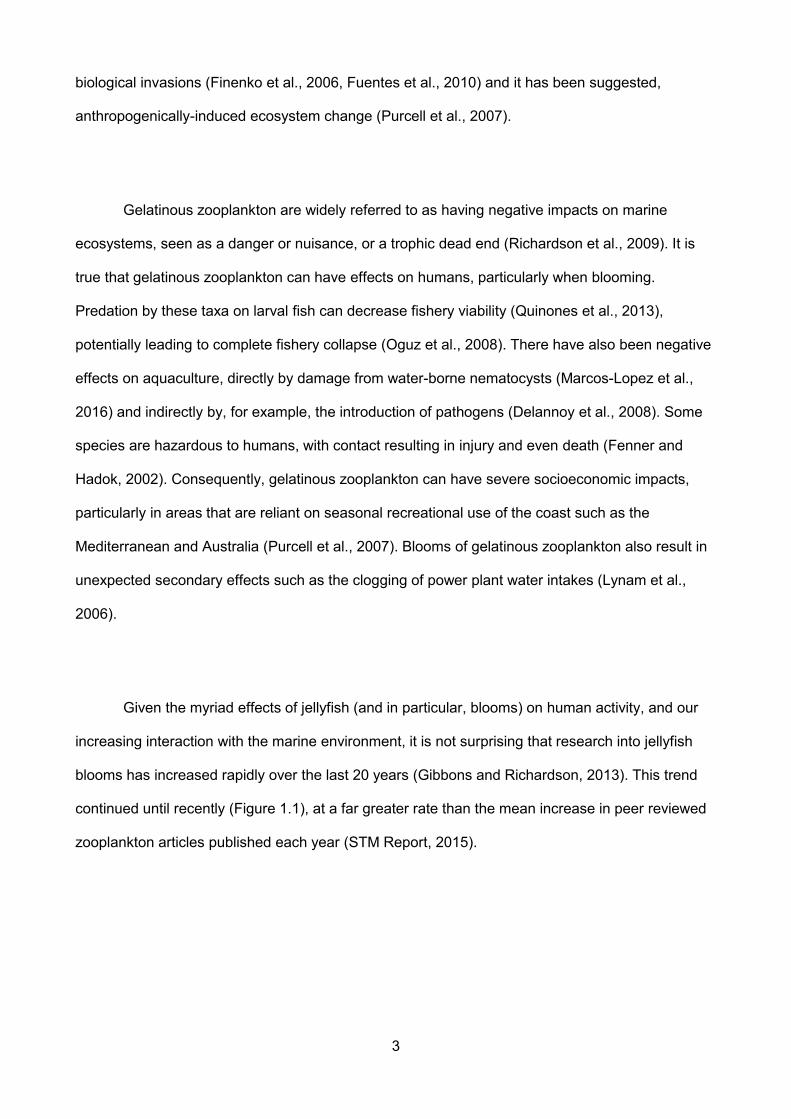
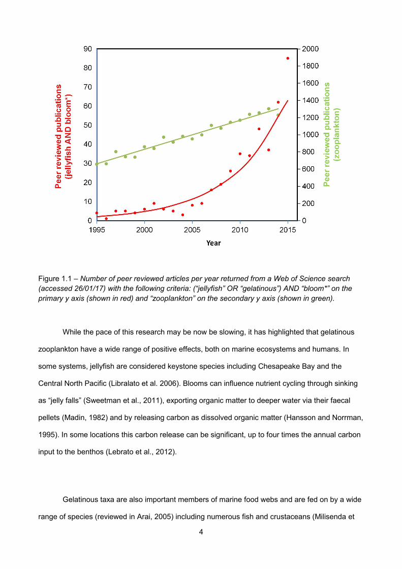
Given the myriad effects of jellyfish (and in particular, blooms) on human activity, and our
increasing interaction with the marine environment, it is not surprising that research into jellyfish
blooms has increased rapidly over the last 20 years (Gibbons and Richardson, 2013). This trend
continued until recently (Figure 1.1), at a far greater rate than the mean increase in peer reviewed
zooplankton articles published each year (STM Report, 2015).
4
Figure 1.1 – Number of peer reviewed articles per year returned from a Web of Science search(accessed 26/01/17) with the following criteria: (“jellyfish” OR “gelatinous”) AND “bloom*” on theprimary y axis (shown in red) and “zooplankton” on the secondary y axis (shown in green).
While the pace of this research may be now be slowing, it has highlighted that gelatinous
zooplankton have a wide range of positive effects, both on marine ecosystems and humans. In
some systems, jellyfish are considered keystone species including Chesapeake Bay and the
Central North Pacific (Libralato et al. 2006). Blooms can influence nutrient cycling through sinking
as “jelly falls” (Sweetman et al., 2011), exporting organic matter to deeper water via their faecal
pellets (Madin, 1982) and by releasing carbon as dissolved organic matter (Hansson and Norrman,
1995). In some locations this carbon release can be significant, up to four times the annual carbon
input to the benthos (Lebrato et al., 2012).
Gelatinous taxa are also important members of marine food webs and are fed on by a wide
range of species (reviewed in Arai, 2005) including numerous fish and crustaceans (Milisenda et
5
al., 2014; D’Ambra et al., 2015), and charismatic megafauna such as marine birds (Harrison, 1984)
and the leatherback turtle, Dermochelyes coriacea (Houghton et al. 2006). Some gelatinous
species (including Cyanea capillata) provide shelter for larval fish in open water, potentially
decreasing mortality of the larvae of commercially important gadoid fish (Lynam and Brierley,
2007).
Humans also use gelatinous zooplankton directly in range of ways. Rhizostomid jellyfish
are fished commercially, with approximately 425,000 tonnes harvested globally (FAO, 1999) with
some jellyfish fisheries actively enriched via stock supplementation (Dong et al. 2010). In folk
medicine, consumption of jellyfish is considered by some to be a cure for a range of conditions
including hypertension and back pain (You et al. 2007) and experimental medical procedures using
jellyfish collagen for treating arthritis and rebuilding damaged tissues have been trialled (Addad et
al., 2011).
A more balanced view of the position and function of gelatinous zooplankton in marine
ecosystems is thus developing. However, the definition of exactly what should be included within
the group remains contentious (Condon et al., 2012). The core groups of the gelatinous
zooplankton include the cnidarian medusae and ctenophores, often referred to collectively as
“jellyfish” (Pitt et al., 2013), on the basis of their comparatively similar structure and relative
phylogenetic proximity. Some authors include salps (Molina-Ramirez et al., 2015), but others
exclude them because of their herbivorous trophic mode (Larson, 1987). Other studies include
chaetognaths (Raskoff et al., 2005), heteropod and pteropod molluscs, appendicularians (Hamner
et al., 1975) and radiolarians (Harbison et al., 1977) as members of the gelatinous zooplankton.
Given the ambiguity of the term gelatinous zooplankton, the word “gelata” has been posed as an
alternative to encompass the full range of plankton with dilute bodies (Haddock, 2004).
6
1.2 - Biological implications of a gelatinous body form
The one trait that unites the various gelatinous taxa is the high percentage of water in their
bodies, expressed as having carbon mass that is approximately 1% (or less) of wet mass (Kiørboe,
2013; Molina Ramirez et al., 2015). Targeted studies on the effects of having a dilute, gelatinous
body form are few, but several authors have suggested that there may be a range of potential
implications on the physiology and ecology of these animals (Hamner et al., 1975, Alldredge, 1984).
Clarke and Peck (1991) highlighted how the energetics of gelatinous zooplankton are more similar
to benthic animals than to other zooplankton, owing to low locomotory and metabolic costs (Gemell
et al., 2013), and lack of lipid stores. Alldredge and Madin (1982) suggested that pelagic tunicates
had higher clearance rates than other zooplankton potentially as a result of their dilute bodies.
Following these studies, other authors began to quantify these differences by modelling the feeding
rate increase associated with an inflated body. Acuña (2001) used filter feeding theory to show that
the salp, Pegea confoederata, would be incapable of meeting its metabolic demand in its nutrient
poor environment if its body were not dilute. Kiørboe (2011) modelled the differences in encounter
areas between a gelatinous organism (0.01 g C cm-3) and a non-gelatinous organism (0.1 g C cm-
3). The increase in carbon mass-specific feeding rate afforded by diluting the body was similar in
magnitude to the increase associated with an organism changing from passive ambush feeding to
an active foraging mode.
This central idea of increasing feeding potential from having a dilute body was later
expanded in a meta-analysis by Acuña et al. (2011). Their study compared the carbon mass-
specific and wet mass-specific respiration and clearance rates of three groups; gelatinous
zooplankton, crustacean zooplankton and fish. Gelatinous zooplankton had similar carbon mass-
specific respiration rates to fish and crustacean zooplankton. This suggested that respiration was a
function of carbon mass, and was unaffected by increasing wet mass. The wet mass-specific
feeding rates of gelatinous zooplankton were similar to those of crustaceans, suggesting that their
feeding methods were equally efficient at the same body volume. In contrast, fish use more
efficient visual foraging, resulting in higher feeding rates at the same wet mass. However, as a
7
result of the low carbon percentage of gelatinous taxa, carbon mass-specific feeding rates were
similar to those of visual foraging fish. In concert, this suggests that gelatinous zooplankton have
higher scope for growth than other zooplankton, with values more similar to those of fish.
The most recent and comprehensive study of the differences between jellyfish (in their
study defined as medusae and ctenophores) and other planktonic animals was carried out by Pitt
et al. (2013). They included comparisons of growth rate, excretion rate, longevity and swimming
velocity with a similar approach to that of Acuña et al. (2011). Pitt et al. (2013) approached the
question by testing whether the carbon and wet mass-specific rates of the gelatinous taxa differed
from the non-gelatinous taxa. Pitt et al. (2011) found that carbon-specific growth rates of gelatinous
zooplankton were 2.2 times those of other zooplankton, and carbon specific ammonium excretion
rates were one tenth of those of other zooplankton.
In the above mentioned comparisons, and indeed in all studies to date investigating the
gelatinous body form, comparisons have been made between those phylogenetic groups that are
classified as gelatinous and those that are not. However, this dichotomy quickly breaks down as
intermediate gelatinous species also exist, such as chaetognaths and pelagic polychaetes
(Kiørboe, 2013). When attempting to analyse the zooplankton as a whole it could be, as I will argue
below, more appropriate to treat degree of dilution as a continuous trait, expressed as carbon
mass as a percentage of wet mass.
1.3 - Aims and layout of this thesis
The relatively few studies comparing highly gelatinous taxa with other zooplankton
demonstrate how tissue dilution can have significant effects on physiological rates such as feeding
and growth. This thesis will investigate whether adopting a continuous approach using carbon
percentage can further our understanding of how dilution affects the biology of zooplankton. A
8
change in thinking from dividing plankton on the basis of gelatinous vs non-gelatinous, to a trait-
based approach which focusses on the continuous variable carbon percentage may seem trivial
but could be a major step forward in a number of ways. First, gelatinous taxa and other
zooplankton currently need to be modelled separately to incorporate the differences in vital rates
described above. This has lead to gelatinous taxa being frequently excluded from ecosystem
models, or being poorly parameterised within them (Pauly et al., 2009). If the differences between
gelatinous and other zooplankton could be related to carbon percentage as a continuous variable,
then variability in vital rates could be included intrinsically without the increase in complexity
associated with dividing the zooplankton into different groups.
Secondly, taxa with different carbon percentages are favoured under different
environmental conditions. For instance, highly gelatinous non visual predators may be more
successful in turbid (Haraldsson et al., 2012) and hypoxic conditions (Thuesen et al., 2005). A
greater understanding of how carbon percentage drives these differences will help us to predict
how planktonic systems will respond to changing environmental conditions, such as increasing
temperature and coastal eutrophication.
Furthermore, understanding carbon percentage as a trait could help us to understand the
evolution of different morphological strategies in the plankton. Seven phyla contain planktonic taxa
that could be considered gelatinous, and understanding the effects of carbon percentage could
help us to better understand why the gelatinous body form is seen in such a wide range of
zooplanktonic organisms.
9
1.3.1 - Aim
The primary aim of this thesis was to address the question: how does tissue dilution affect
the biology of zooplankton?
1.3.2 - Objectives
To achieve this aim I have investigated whether the differences in growth and ingestion rate
between gelatinous and other zooplankton are a consequence of differences in carbon percentage.
A range of different approaches were used including meta-analysis, experiments and analysis of
time series data. The aim was completed through a series of sequential objectives, namely:
(I) – HOW DO WE EXPECT CARBON PERCENTAGE TO INFLUENCE ENERGY BUDGETS?
In Chapter 2, by applying established scaling theory I have explored how carbon
percentage is expected to influence the respiration, feeding and growth rates of zooplankton.
These predictions are used as support for the hypotheses advanced in the subsequent chapters.
Also within Chapter 2, the sampling protocol at the L4 sampling station is detailed to provide
background for the use of the zooplankton abundance time series in Chapters 3, 5, 6 and 7.
(I) – IS CARBON PERCENTAGE CONTINUOUS?
In Chapter 3, synchronous measurements of carbon and wet masses of a wide range of
zooplanktonic taxa were compiled from the literature. A meta-analysis of these collected data was
used to investigate the distribution of species along the axis of carbon percentage. By assessing to
what extent the carbon percentages of zooplankton form a natural division between discrete
gelatinous and non-gelatinous groups, I determined whether it was appropriate to treat carbon
percentage as a continuous trait. This meta-analysis provided information on the potential variation
in traits but the range of species analysed was not representative of the species that inhabit any
single ecosystem. For this reason, zooplankton abundance time series data from the Plymouth L4
sampling station (detailed in Chapter 2) was used to determine how biomass was distributed along
the axis of carbon percentage in a real assemblage.
10
(II) – IS CARBON PERCENTAGE RELATED TO GROWTH RATE?
Chapter 3 continued by combining the carbon percentage values with a meta-analysis of
published zooplankton growth rates to determine whether carbon percentage was related to growth
rate. Carbon percentage was combined with carbon mass (alongside standardisations for food and
temperature) to provide a unified model of zooplankton growth. The data were also tested for a
relationship between carbon percentage and carbon mass, both in the meta-analysis and the real
assemblage at L4.
(III) – IS CARBON PERCENTAGE FIXED WITHIN A SPECIES?
Chapter 3 explored whether interspecific variability in carbon percentage affected the
biology of zooplankton. Chapter 4 extends the investigation to intraspecific variability using a
series of experiments on ephyra larvae of the moon jellyfish, Aurelia aurita. The carbon and wet
masses of the growing ephyrae were measured to determine whether carbon percentage varies
through early development.
(IV) – HOW DOES INTRASPECIFIC VARIATION IN CARBON PERCENTAGE AFFECT FEEDING
AND GROWTH RATES?
Following on from objective iii, Chapter 4 determined whether variability in carbon
percentage through ontogeny influences the feeding and growth rates of ephyrae. The ephyrae
were incubated in saturating food conditions, and ingestion and growth rates were measured and
related to carbon percentage and carbon mass. A simple mechanistic model was constructed to
further explore how variation in carbon percentage affects the energy budget of the ephyrae.
11
(V) – DOES CARBON PERCENTAGE AFFECT THE FORMATION OF JELLYFISH BLOOMS?
Previous studies have suggested that gelatinous taxa have higher carbon specific feeding
and growth rates than other zooplankton. Chapter 5 investigated whether these organismal
differences manifest at the population level by asking whether carbon percentage is related to the
formation of rapid population increases i.e. blooms. Using zooplankton abundance from the L4
time series, Chapter 5 also determined whether carbon percentage affects variability in abundance
and population increase rate among the zooplankton.
(VI) WHAT IS THE RELATIONSHIP BETWEEN CARBON PERCENTAGE AND CARBON MASS?
A relationship between carbon mass and carbon percentage was established in Chapter 3, and
was explored in greater detail in Chapter 6. By investigating the variability in this relationship,
Chapter 6 suggested how carbon mass and carbon percentage interact to set constraints on
zooplankton body size.
(VII) WHAT DOES THIS MEAN FOR HOW WE THINK ABOUT ZOOPLANKTON AND CARBON
PERCENTAGE?
Chapter 7 summarised how the results found in the other chapters could change the way
we think about zooplankton. Additionally, Chapter 7 explored how carbon percentage might be
used in different way in future studies, for instance as a response variable for summarising
planktonic assemblages.

12
13
CHAPTER 2 – Theoretical model of the effects of carbon
percentage and L4 sampling details
14
2.1 - Introduction
Throughout this thesis I have used a theoretical model to make predictions about the
effects of carbon percentage on various aspects of zooplankton biology. In this chapter I develop
the form and explain the assumptions of this model. To test some of the predictions posed by the
model and investigate population level phenomena, the L4 time series of zooplankton abundance
has been used. The background information and sampling regime for this time series are detailed
below.
2.2 - Dilution as a continuous trait: modelling the potential effects of carbon percentage
Using the differences between gelatinous and non-gelatinous zooplankton presented in
Chapter 1 and scaling theory, it is possible to predict how carbon percentage (C% = carbon mass
as a percentage of wet mass) might affect vital rates using a simple geometric model.
The most immediate effect of variation in carbon percentage is on effective body size (i.e.
body volume). Two organisms of the same carbon mass but different carbon percentages will have
different wet masses, and therefore different effective body sizes. As body size is integral to the
biology of all organisms, hypotheses for the effects of carbon percentage will be formulated by
applying existing knowledge of how changing body size alters vital rates. The model below will
compare two organisms of the same carbon mass, C, but different wet masses, WM. For the sake
of comparison, these organisms will be referred to as gelatinous and non-gelatinous, and represent
opposite ends of the range of carbon percentage.
The non-gelatinous organism has a “normal” carbon percentage (C = 10% WM);
(eq. 1.1) WM = C / 0.1
The gelatinous organism has a lower carbon percentage (C = 0.1% WM);
(eq. 1.2) WM = C / 0.001
15
As “body size” is described as the primary biological trait determining energy budgets
(Andersen et al., 2016), we can use different metrics of body size to estimate a range of energy
budget parameters for these two organisms. In the following paragraphs I have applied established
scaling theory to our current understanding of how gelatinous zooplankton differ from other
planktonic taxa (Acuña et al., 2011; Pitt et al, 2013). By combining this with a logical exploration of
whether energy budget parameters are likely to be controlled by carbon or wet mass, I have
developed a range of predictions of how carbon percentage might influence the energy budget of
zooplankton. These predictions are tested using a range of methods in subsequent chapters.
2.2.1 - Respiration
Water does not have respiratory demand (or capability) so therefore respiration can only be
a function of the organic content of the body (Acuña et al., 2011). The organic content or
metabolically active mass is represented here as carbon mass, therefore in both cases;
(eq. 1.3) Respiration rate = aCb
Respiration rate is a function of carbon mass, C, a constant, a, and the body mass scaling
exponent, b. The value of the body mass scaling exponent of metabolism, b, has been a topic of
much debate for nearly a century (Kleiber, 1932). However, as we are comparing organisms of
identical carbon mass, the values of the exponent and the coefficient do not affect the model. As
respiration is a function of carbon mass (and is not affected by wet mass, Acuña et al., 2011), the
respiration of the gelatinous and non-gelatinous organisms in the model will be equal.
2.2.2 - Ingestion rate
Ingestion rate is a complex variable that can vary widely depending on feeding mode, food
concentration, prey type and a wide range of other factors. For the sake of simplicity, it is assumed
that both organisms are neutrally buoyant, ambush feeders that do not actively forage. Following
16
these assumptions, ingestion rate is a function of encounter rate, which is in turn a function of
surface area, and therefore the following equation will apply;
(eq. 1.4) Ingestion rate = x(C/C%)2/3
The constant, x, will be dependent on feeding mode and the other factors mentioned above,
and is not critical for this investigation. The scaling exponent of b = 2/3 is a consequence of
surface area scaling as length2 and volume scaling as length3.
From this point the gelatinous and non-gelatinous organisms diverge;
(eq. 1.5) Non-gelatinous feeding rate = (C/0.1)2/3 = (10C)2/3
(eq. 1.6) Gelatinous feeding rate = (C/0.001)2/3 = (1000C)2/3
Both surface area and volume are functions of wet mass, and therefore feeding rate differs
between the gelatinous and non-gelatinous organisms. It could be argued that given the wide
variety of feeding modes that exist, modelling ingestion rate using surface area is too great an
assumption. However, the purpose of this model is not to produce quantitative estimates of the
effect of carbon percentage, but to suggest the form of this relationship for testing in subsequent
chapters. In the case of feeding rate, scaling exponents of b < 0 are very rare both interspecifically
(Kiørboe and Hirst, 2014) and intraspecifically (Hirst and Forster, 2013), and b values typically vary
between 0.66 and 1. With this in mind, it is predicted that decreasing carbon percentage will
typically increase carbon-specific ingestion rate. In this model, the gelatinous organism will have
higher carbon specific ingestion rates than the non-gelatinous, with the difference between the two
depending on carbon mass and the difference in carbon percentage.
17
2.2.3 - Scope for growth
Scope for growth is an estimate of the energy available for growth, it is a function of feeding
rate minus respiratory cost;
(eq. 1.7) Scope for growth = food intake – respiration loss = (C/C%)2/3 – Cb
Therefore;
(eq. 1.8) Non-gelatinous growth = (10C)2/3 – Cb
(eq. 1.9) Gelatinous growth = (1000C)2/3 – Cb
As shown above, while the carbon specific respiration rate of the gelatinous and non-
gelatinous organisms is the same, carbon specific feeding rate differs and therefore scope for
growth differs also. The scope for growth of the gelatinous organism is higher than that of the non-
gelatinous organism, with the magnitude of the difference dependent on carbon mass. Scope for
growth does not equal growth rate, but as an estimate of the resources available for growth can be
used to estimate relative growth rate.
2.3 - Introduction to the Western Channel Observatory
The Western Channel Observatory is the collective name given to a series of atmospheric,
planktonic and benthic monitoring and process stations in the shelf waters south of Plymouth
(Figure 2.1). The centrepiece stations are known as L4 (13 km SSW of Plymouth) and E1 (40 km
SSW of Plymouth) which are in water depths respectively of ~54 and 75 m. These stations have
been sampled periodically for over a century (Southward et al., 2005), but zooplankton sampling at
L4 was resumed on a weekly basis by Plymouth Marine Laboratory in March 1988. It thus provides
a particularly valuable time series and the zooplankton data set used in my study.
18
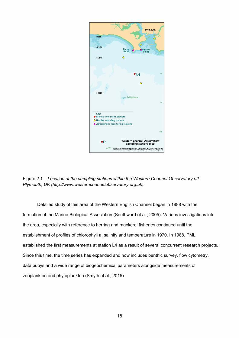
Figure 2.1 – Location of the sampling stations within the Western Channel Observatory offPlymouth, UK (http://www.westernchannelobservatory.org.uk).
Detailed study of this area of the Western English Channel began in 1888 with the
formation of the Marine Biological Association (Southward et al., 2005). Various investigations into
the area, especially with reference to herring and mackerel fisheries continued until the
establishment of profiles of chlorophyll a, salinity and temperature in 1970. In 1988, PML
established the first measurements at station L4 as a result of several concurrent research projects.
Since this time, the time series has expanded and now includes benthic survey, flow cytometry,
data buoys and a wide range of biogeochemical parameters alongside measurements of
zooplankton and phytoplankton (Smyth et al., 2015).

19
The work that has been made possible as a result of the observatory has been varied and
impactful (summarised in Smyth et al., 2015). Studies from the observatory have enhanced our
knowledge of plankton ecology over the full range of biological scales, from viral interactions
(Nizzimov et al., 2015) to the effects of microplastics (Cole et al., 2015). One of the key sampling
efforts that takes place at the observatory is the L4 zooplankton time series. This provides a rich
dataset that began in 1988, and since then has expanded to weekly recordings of the abundance
of 199 taxa. As a result of this time series, there is a good understanding of zooplankton dynamics
at L4 (Eloire et al., 2010). Zooplankton abundance peaks in April and September, driven by
abundant phytoplankton and temperature. The assemblage is dominated by copepods, with seven
of the ten species with the highest average abundance at L4 belonging to this group. Diversity
varies throughout the year. In winter, most of the zooplankton sampled come from a fairly narrow
group of primarily crustacean taxa. In the summer the assemblage is much more diverse, with
abundance distributed more evenly through a wide range of taxa. Meroplanktonic larvae contribute
significantly to the assemblage at L4 at specific times of year, with cirripedes, echinoderm larvae
and bivalve larvae occurring in high numbers in spring, summer and autumn respectively. Also,
several gelatinous taxa, particularly siphonophores and ctenophores, can form the majority of the
sampled assemblage for short periods during summer.
A key strength of the L4 zooplankton time series is the weekly resolution, which has
allowed researchers to investigate the formation and timing of seasonal events (Atkinson et al.,
2015). In this thesis I have used the L4 time series in a similar manner to investigate population
level traits of zooplankton in chapters 3, 5, 6 and 7. As these data have been used in multiple
chapters, I have detailed the sampling protocol and method below to avoid repetition.
2.3.1 - L4 zooplankton time series sampling
Sampling at the L4 site consists of a pair of vertical hauls with a 200 µm WP2 zooplankton
net from 50 m to the surface (maximum depth 54m). The nets are retrieved at 20 cm s-1 and are
20
immediately fixed in 4% formaldehyde solution in 0.2 µm filtered seawater (Maud et al., 2015).
Mesozooplankton from the formalin-preserved vertical net hauls are enumerated and identified by
microscopy. Two sub-samples of different size are analysed per sample. The smaller one is taken
with a Stempel pipette for the abundant taxa. Typical subsamples ranged from 1-10ml from 300 ml.
A second, larger aliquot is analysed for rarer and large taxa, typically 12.5%, 25% or 50% (Eloire et
al., 2010). Abundances across the two hauls were averaged and numbers expressed as
individuals per m3 allowing for a 95% net filtration efficiency (UNESCO, 1968). Some species are
enumerated further according to maturity stage, e.g. Calanus helgolandicus copepodites CI-CV
and Calanus helgolandicus adults. For the purposes of my analyses, these groups were combined
to yield a single value for each taxon at each time point. To estimate biomass of each zooplankton
taxon (mg C m-3) from numerical density (no. m-3), a total of 3780 individuals of the dominant taxa
from the formalin-preserved catches at L4 taken throughout 2014 and 2015 were measured. From
standard length measurements (e.g. cnidarian bell height or diameter, copepod prosome length),
length-carbon mass relationships from the literature were used to estimate carbon masses per
individual. The derived values were then averaged into seasons, namely spring (March-May),
summer (June-August), autumn (September-November) and winter (December to February) to
account for the high intraspecific variability in length observed at L4 (Atkinson et al., 2015). From
this, season-specific mean carbon masses per individual were derived, which were multiplied by
numerical densities to estimate biomass density (mg C m-3). Previously measured L4-specific
seasonal values of individual carbon biomass were used when available (e.g. Calanus
helgolandicus; Pond et al., 1996).
21
CHAPTER 3 – Disentangling the counteracting effects of
water content and carbon mass on zooplankton growth
This chapter was published as the following reference and is appended at the end of this volume;McConville, K., Atkinson, A., Fileman, E.S., Spicer, J.I. and Hirst, A.G., 2016. Disentanglingthe counteracting effects of water content and carbon mass on zooplankton growth. Journal ofPlankton Research 39 246-256.
22
3.1 - Introduction
Gelatinous zooplankton have been attracting increasing attention from scientists and the
popular press alike, and the current literature tends to emphasise the differences between
gelatinous taxa and other zooplankton (e.g. Richardson et al., 2009; Kiørboe et al., 2011; Gibbons
and Richardson, 2013). This chapter takes a different approach by investigating whether carbon
percentage can be treated as a continuous variable, and whether a relationship exists between
carbon percentage and growth rate. Based on a compilation of body composition data, Kiørboe
(2013) found that most zooplankton species are either gelatinous (carbon mass ~0.5% of wet
mass) or not gelatinous (5-10%), with comparatively few intermediates. Much recent research has
been directed toward comparing and contrasting gelatinous versus non-gelatinous zooplankton.
For example, compared to other planktonic animals, gelatinous zooplankton have higher carbon
mass-specific feeding rates (Hamner et al., 1975; Acuña, 2001; Acuña et al., 2011), lower
locomotion costs and higher specific growth rates (Hirst et al., 2003; Pitt et al., 2013). Indeed,
gelatinous taxa such as salps are amongst the fastest growing metazoans (Bone, 1998).
The use of a categorical approach to zooplankton body composition (i.e. gelatinous versus
non-gelatinous) contrasts with the treatment of carbon mass (Peters, 1983), which is used as a
continuous variable in many models of growth (Hansen et al., 1997; Gillooly et al., 2002; Hirst et al.
2003). However, the carbon percentage of zooplankton species also varies widely, even among
gelatinous taxa (Molina-Ramirez et al., 2015). A recent review suggested that water content was
second only to body size in determining key aspects of the biology of zooplankton (Andersen et al.,
2015b). So far, empirical models of zooplankton growth use equations that are specific to various
taxonomic groups (e.g. Hirst et al., 2003; Kiørboe and Hirst, 2014) and these equations have not
yet been unified. As carbon mass and carbon percentage are capable of varying independently, it
is important to consider them together in empirical models of zooplankton growth. Furthermore,
quantifying the relationship between growth rate and carbon percentage may help to explain how
carbon percentage functions as an evolutionary trait, and, for example, why there are gelatinous
representatives from six phyla found in the plankton.
23
In this chapter, I have used both a meta-analyses approach and an in situ time series of
zooplankton abundance data from weekly sampling at the Plymouth L4 time series (detailed in
Chapter 2). The first step was to quantify the degree of variability in carbon percentage both in
“trait space” from the meta-analysis dataset and in a natural plankton assemblage, to gauge
whether it was appropriate to treat water content as a continuous variable. The second aim was to
investigate the degree of collinearity between carbon mass and carbon percentage, again both in a
meta-assemblage and in the L4 assemblage. Dependent on the outcome of these two objectives,
the third was to construct a model of zooplankton growth that combines carbon mass and carbon
percentage to provide a simplified prediction of growth for modellers and empiricists.
3.2 - Methods
3.2.1 - Carbon percentage data
Ratios of carbon mass to wet mass were combined from a series of recent compilations
(Kiørboe, 2013; Pitt et al., 2013; Molina-Ramirez et al., 2015). The amalgamated dataset with
sources is presented in Appendix I. Only concurrent measurements of carbon and wet mass of the
same individual were used to calculate carbon percentage.
The degree of tissue dilution of zooplankton taxa has been expressed previously as body
carbon content (Molina-Ramirez et al., 2015). However, to avoid confusion with carbon mass,
throughout my thesis it is referred to as “carbon percentage” (carbon mass as a percentage of wet
mass). The levels of taxonomic organisation used for comparison were selected based on
functional diversity and body form (e.g. phylum for Chaetognatha, but orders Cydippida and
Lobata).
24
3.2.2 – Analysis of the zooplankton assemblage from the L4 site
The sampling, subsampling protocol and environment of the L4 time series are detailed in
section 2.3. Of the approximately 189 taxa recorded at L4, only 22 contributed more than 0.5% to
the total estimated biomass for all species. To examine how biomass was distributed across the
spectrum of carbon percentage, these taxa were assigned to log2 classes (0.1 - 0.2%, 0.2 – 0.4%,
0.4 – 0.8%, 0.8 – 1.6%, 1.6 – 3.2%, 3.2 – 6.4%, 6.4 – 12.8%, > 12.8%) using the carbon
percentage data in Appendix I. The distribution of carbon biomass in each carbon percentage
category across the seasons was then calculated.
3.2.3 - Growth rate data
Using the references from the appendices of Kiørboe and Hirst (2014) as a starting point,
zooplankton growth rate data were extracted from the original sources and augmented by
searching the literature (Appendix II). To improve comparability of source data I restricted the
meta-analysis to data from laboratory incubations with food available in high (assumed non-limiting)
concentrations. By using only data collected under these conditions I suggest that the
measurements are more directly comparable, with the observed patterns more likely to reflect the
intrinsic biology of the species than external factors.
Published growth rates are normally expressed either as increase in length or body mass
over time. When organism size was expressed as length, published length-mass regressions were
used to convert to body carbon mass (Hirst, 2012; Kiørboe and Hirst, 2014). To express growth
rates in the terms commonly used for zooplankton (as an exponential rate; see Hirst and Forster,
2013), the mass-specific growth rate, g (d-1) was determined as:
(eq. 2.1) g = (ln Mt – ln M0)/d
Mt is mass at time t, M0 is mass at the previous time point, and d is the time period between
the two measurements of mass (in days).
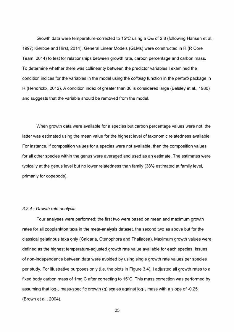
25
Growth data were temperature-corrected to 15oC using a Q10 of 2.8 (following Hansen et al.,
1997; Kiørboe and Hirst, 2014). General Linear Models (GLMs) were constructed in R (R Core
Team, 2014) to test for relationships between growth rate, carbon percentage and carbon mass.
To determine whether there was collinearity between the predictor variables I examined the
condition indices for the variables in the model using the colldiag function in the perturb package in
R (Hendrickx, 2012). A condition index of greater than 30 is considered large (Belsley et al., 1980)
and suggests that the variable should be removed from the model.
When growth data were available for a species but carbon percentage values were not, the
latter was estimated using the mean value for the highest level of taxonomic relatedness available.
For instance, if composition values for a species were not available, then the composition values
for all other species within the genus were averaged and used as an estimate. The estimates were
typically at the genus level but no lower relatedness than family (38% estimated at family level,
primarily for copepods).
3.2.4 - Growth rate analysis
Four analyses were performed; the first two were based on mean and maximum growth
rates for all zooplankton taxa in the meta-analysis dataset, the second two as above but for the
classical gelatinous taxa only (Cnidaria, Ctenophora and Thaliacea). Maximum growth values were
defined as the highest temperature-adjusted growth rate value available for each species. Issues
of non-independence between data were avoided by using single growth rate values per species
per study. For illustrative purposes only (i.e. the plots in Figure 3.4), I adjusted all growth rates to a
fixed body carbon mass of 1mg C after correcting to 15oC. This mass correction was performed by
assuming that log10 mass-specific growth (g) scales against log10 mass with a slope of -0.25
(Brown et al., 2004).
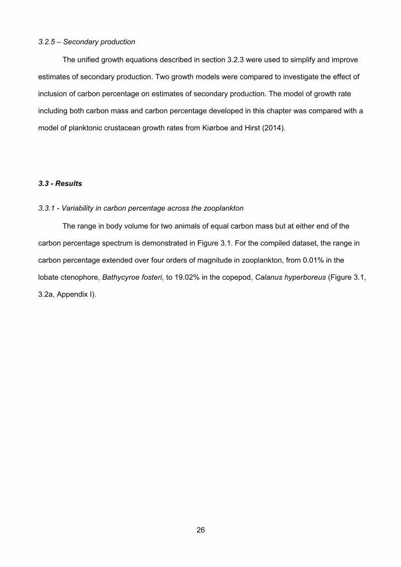
26
3.2.5 – Secondary production
The unified growth equations described in section 3.2.3 were used to simplify and improve
estimates of secondary production. Two growth models were compared to investigate the effect of
inclusion of carbon percentage on estimates of secondary production. The model of growth rate
including both carbon mass and carbon percentage developed in this chapter was compared with a
model of planktonic crustacean growth rates from Kiørboe and Hirst (2014).
3.3 - Results
3.3.1 - Variability in carbon percentage across the zooplankton
The range in body volume for two animals of equal carbon mass but at either end of the
carbon percentage spectrum is demonstrated in Figure 3.1. For the compiled dataset, the range in
carbon percentage extended over four orders of magnitude in zooplankton, from 0.01% in the
lobate ctenophore, Bathycyroe fosteri, to 19.02% in the copepod, Calanus hyperboreus (Figure 3.1,
3.2a, Appendix I).
27
Figure 3.1 - Comparison of the relative carbon (black) and wet masses (grey) of Calanushyperboreus (left, carbon percentage = 19.02%) and Bathycyroe fosteri (right, carbon percentage =0.01%). The relative area of each shade is scaled as volume so the silhouettes are representativeof true size.

28
The intervals between adjacent ranked species were small relative to the range covered
(Figure 3.2a), suggesting that water content could be considered as a continuous variable.
Figure 3.2 - (a) Zooplankton species ranked according to their carbon percentage (CM%WM; log10scale), each horizontal bar represents a single species. Colours indicate taxonomic groups asdetailed in the legend. (b) Zooplankton taxonomic groups ranked according to their carbon mass(as % of wet mass; log10 scale). Boxes indicate median, lower and upper quartiles with whiskersshowing the range. (Vertical lines at 0.5 and 5 CM%WM represent the composition of thegelatinous and non-gelatinous taxa defined by Kiørboe, 2013).
29
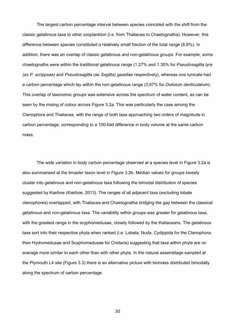
30
The largest carbon percentage interval between species coincided with the shift from the
classic gelatinous taxa to other zooplankton (i.e. from Thaliacea to Chaetognatha). However, this
difference between species constituted a relatively small fraction of the total range (6.8%). In
addition, there was an overlap of classic gelatinous and non-gelatinous groups. For example, some
chaetognaths were within the traditional gelatinous range (1.27% and 1.35% for Pseudosagitta lyra
(as P. scrippsae) and Pseudosagitta (as Sagitta) gazellae respectively), whereas one tunicate had
a carbon percentage which lay within the non-gelatinous range (3.87% for Doliolum denticulatum).
This overlap of taxonomic groups was extensive across the spectrum of water content, as can be
seen by the mixing of colour across Figure 3.2a. This was particularly the case among the
Ctenophora and Thaliacea, with the range of both taxa approaching two orders of magnitude in
carbon percentage, corresponding to a 100-fold difference in body volume at the same carbon
mass.
The wide variation in body carbon percentage observed at a species level in Figure 3.2a is
also summarised at the broader taxon level in Figure 3.2b. Median values for groups loosely
cluster into gelatinous and non-gelatinous taxa following the bimodal distribution of species
suggested by Kiørboe (Kiørboe, 2013). The ranges of all adjacent taxa (excluding lobate
ctenophores) overlapped, with Thaliacea and Chaetognatha bridging the gap between the classical
gelatinous and non-gelatinous taxa. The variability within groups was greater for gelatinous taxa,
with the greatest range in the scyphomedusae, closely followed by the thaliaceans. The gelatinous
taxa sort into their respective phyla when ranked (i.e. Lobata, Nuda, Cydippida for the Ctenophora,
then Hydromedusae and Scyphomedusae for Cnidaria) suggesting that taxa within phyla are on
average more similar to each other than with other phyla. In the natural assemblage sampled at
the Plymouth L4 site (Figure 3.3) there is an alternative picture with biomass distributed bimodally
along the spectrum of carbon percentage.

31
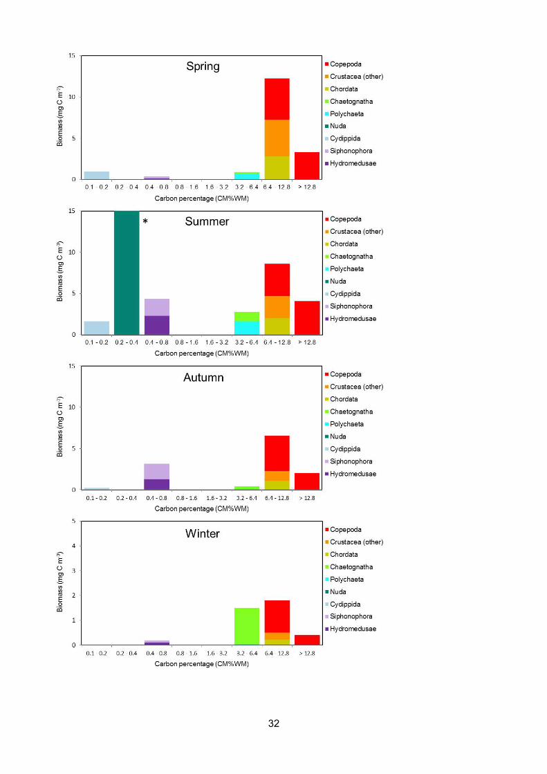
32

33
Figure 3.3 - Distribution of carbon biomass (mg C m-3) between log2 carbon percentage categoriesthrough spring, summer, autumn and winter (2009-2015) at the L4 sampling site, Western ChannelObservatory, Plymouth. The same colour coding of taxa is used as in Figure 3.1 – see legend. * -Biomass value for the category 0.4 – 0.8 exceeds the scale in summer (crudely estimated at 34 mgC m-3) as a result of 7 high abundance observations of Beroe spp. (of total 318 time-points). Upperlimit of biomass scale in winter is 5 mg C m-3.
The biomass was primarily concentrated in the categories that are either highly gelatinous
(carbon mass 0.1 – 0. 8% of wet mass) or non-gelatinous (6.4 - > 12.8%). However, there is
considerable variability within the carbon percentage categories, as some gelatinous taxa are as
much as 8 times larger in wet mass for the same carbon mass as others. The biomass in the
intermediate categories (0.8 – 1.6% and 1.6 – 3.2%) was very low and below our threshold for
inclusion. This area of the spectrum is populated by thaliaceans and large rhizostomid
scyphomedusae, which are not commonly recorded at L4 and may be poorly sampled by the
0.57m mouth diameter (200µm mesh) nets used. Gelatinous taxa comprised a greater proportion
of biomass in summer than the other seasons. In winter, chaetognaths (carbon mass 3.56% of wet
mass) have similar total biomass to the dominant copepods. There is also a broad trend of
increasing carbon percentage through the year within the gelatinous taxa. In spring, the cydippids
(the most gelatinous group frequently encountered at L4) are dominant, followed by Nuda (Beroe)
in summer and finally hydromedusae and siphonophores in autumn.
3.3.2 - Relationship between carbon mass and carbon percentage
Based on the meta-analysis datasets there was a negative relationship between carbon
mass and carbon percentage (Figure 3.4).
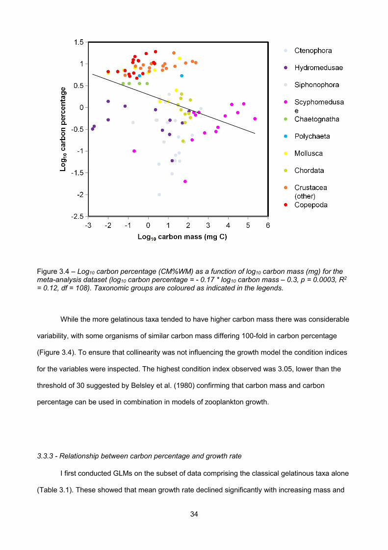
34
Figure 3.4 – Log10 carbon percentage (CM%WM) as a function of log10 carbon mass (mg) for themeta-analysis dataset (log10 carbon percentage = - 0.17 * log10 carbon mass – 0.3, p = 0.0003, R2
= 0.12, df = 108). Taxonomic groups are coloured as indicated in the legends.
While the more gelatinous taxa tended to have higher carbon mass there was considerable
variability, with some organisms of similar carbon mass differing 100-fold in carbon percentage
(Figure 3.4). To ensure that collinearity was not influencing the growth model the condition indices
for the variables were inspected. The highest condition index observed was 3.05, lower than the
threshold of 30 suggested by Belsley et al. (1980) confirming that carbon mass and carbon
percentage can be used in combination in models of zooplankton growth.
3.3.3 - Relationship between carbon percentage and growth rate
I first conducted GLMs on the subset of data comprising the classical gelatinous taxa alone
(Table 3.1). These showed that mean growth rate declined significantly with increasing mass and
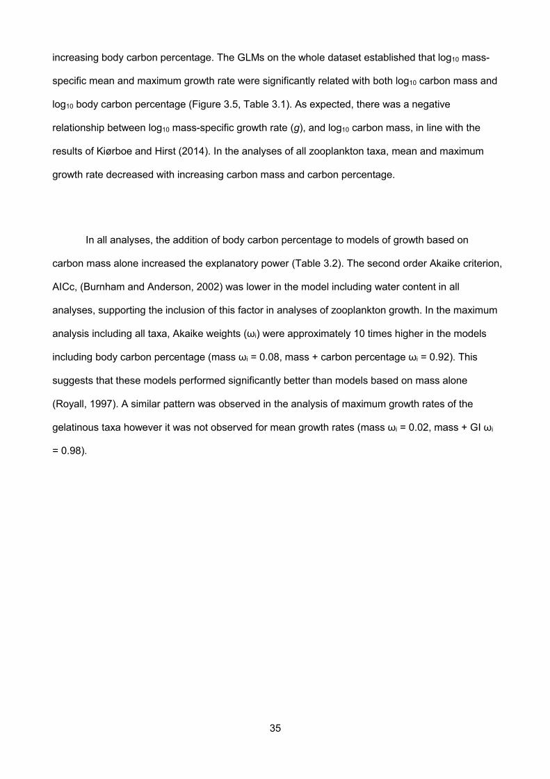
35
increasing body carbon percentage. The GLMs on the whole dataset established that log10 mass-
specific mean and maximum growth rate were significantly related with both log10 carbon mass and
log10 body carbon percentage (Figure 3.5, Table 3.1). As expected, there was a negative
relationship between log10 mass-specific growth rate (g), and log10 carbon mass, in line with the
results of Kiørboe and Hirst (2014). In the analyses of all zooplankton taxa, mean and maximum
growth rate decreased with increasing carbon mass and carbon percentage.
In all analyses, the addition of body carbon percentage to models of growth based on
carbon mass alone increased the explanatory power (Table 3.2). The second order Akaike criterion,
AICc, (Burnham and Anderson, 2002) was lower in the model including water content in all
analyses, supporting the inclusion of this factor in analyses of zooplankton growth. In the maximum
analysis including all taxa, Akaike weights (ωi) were approximately 10 times higher in the models
including body carbon percentage (mass ωi = 0.08, mass + carbon percentage ωi = 0.92). This
suggests that these models performed significantly better than models based on mass alone
(Royall, 1997). A similar pattern was observed in the analysis of maximum growth rates of the
gelatinous taxa however it was not observed for mean growth rates (mass ωi = 0.02, mass + GI ωi
= 0.98).
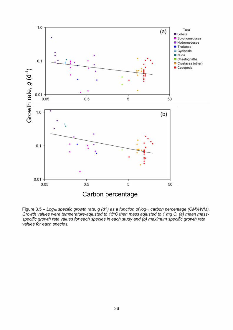
36
Figure 3.5 – Log10 specific growth rate, g (d-1) as a function of log10 carbon percentage (CM%WM).Growth values were temperature-adjusted to 15oC then mass adjusted to 1 mg C. (a) mean mass-specific growth rate values for each species in each study and (b) maximum specific growth ratevalues for each species.
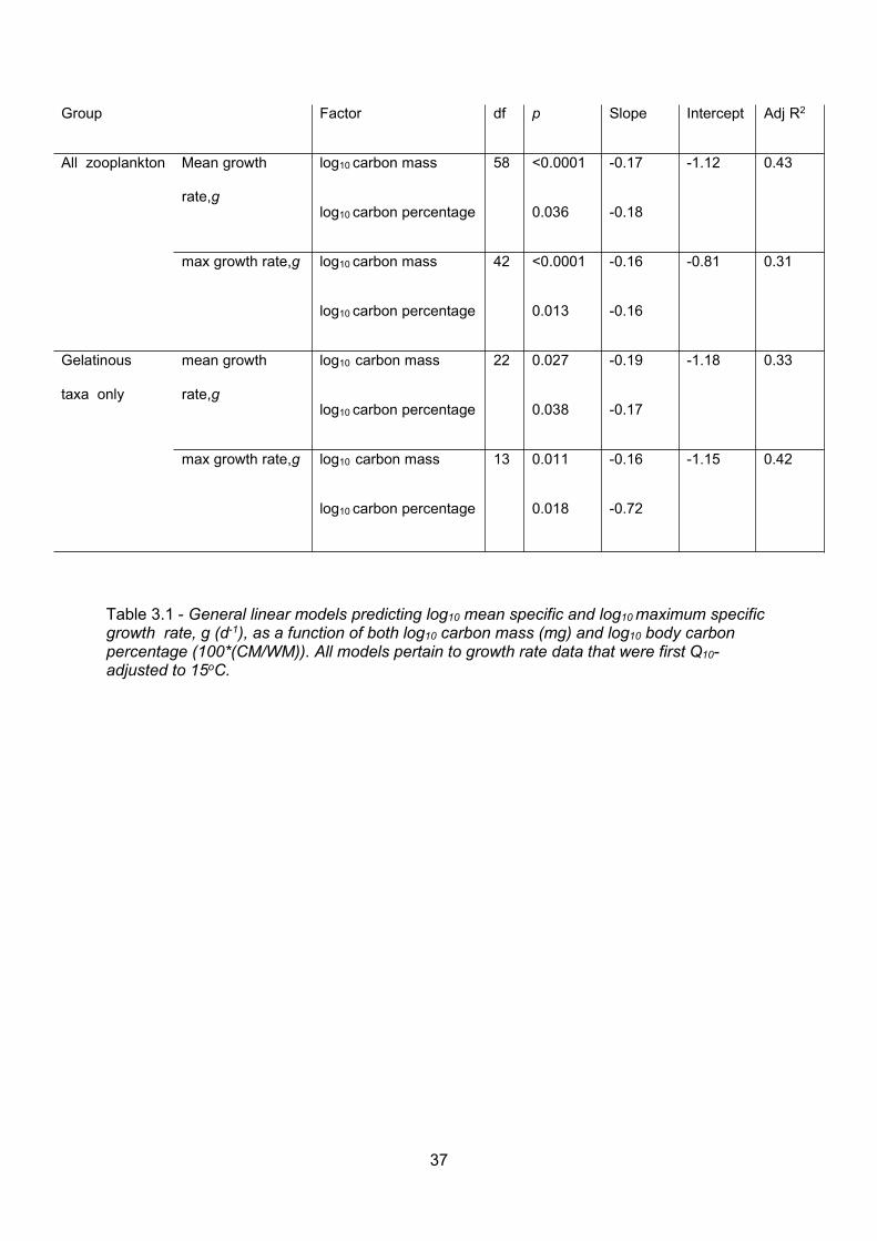
37
Group Factor df p Slope Intercept Adj R2
All zooplankton Mean growth
rate,g
log10 carbon mass 58 <0.0001 -0.17 -1.12 0.43
log10 carbon percentage 0.036 -0.18
max growth rate,g log10 carbon mass 42 <0.0001 -0.16 -0.81 0.31
log10 carbon percentage 0.013 -0.16
Gelatinous
taxa only
mean growth
rate,g
log10 carbon mass 22 0.027 -0.19 -1.18 0.33
log10 carbon percentage 0.038 -0.17
max growth rate,g log10 carbon mass 13 0.011 -0.16 -1.15 0.42
log10 carbon percentage 0.018 -0.72
Table 3.1 - General linear models predicting log10 mean specific and log10maximum specificgrowth rate, g (d-1), as a function of both log10 carbon mass (mg) and log10 body carbonpercentage (100*(CM/WM)). All models pertain to growth rate data that were first Q10-adjusted to 15oC.
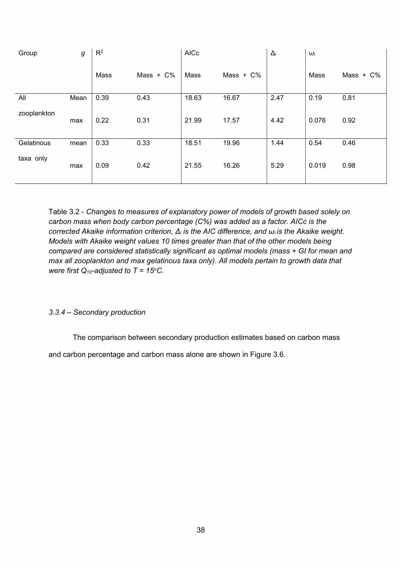
38
Table 3.2 - Changes to measures of explanatory power of models of growth based solely oncarbon mass when body carbon percentage (C%) was added as a factor. AICc is thecorrected Akaike information criterion, Δi is the AIC difference, and ωi is the Akaike weight.Models with Akaike weight values 10 times greater than that of the other models beingcompared are considered statistically significant as optimal models (mass + GI for mean andmax all zooplankton and max gelatinous taxa only). All models pertain to growth data thatwere first Q10-adjusted to T = 15oC.
3.3.4 – Secondary production
The comparison between secondary production estimates based on carbon mass
and carbon percentage and carbon mass alone are shown in Figure 3.6.
Group g R2 AICc Δi ωi
Mass Mass + C% Mass Mass + C% Mass Mass + C%
All
zooplankton
Mean 0.39 0.43 18.63 16.67 2.47 0.19 0.81
max 0.22 0.31 21.99 17.57 4.42 0.076 0.92
Gelatinous
taxa only
mean 0.33 0.33 18.51 19.96 1.44 0.54 0.46
max 0.09 0.42 21.55 16.26 5.29 0.019 0.98

39
Figure 3.6 – Illustrative estimates of maximum secondary production at the L4 sampling site at weekly resolution between 05/01/2009 and15/12/2012. Growth rates were estimated on the basis of carbon mass alone (log10 carbon specific growth rate (mg C mg C-1 h-1) = - 2.82 - 0.31log10 carbon mass(mg)) using the equation for crustaceans from Kiørboe and Hirst (2014) and carbon mass alongside carbon percentage(log10 specific growth rate, g, ((d-1) - 0.81 - 0.16 log10 carbon mass (mg) - 0.16 log10 carbon percentage ((CM/WM)*100) using the maximumgrowth rate equation for all zooplankton shown in Table 3.1. Growth rates were temperature adjusted using a Q10 of 2.8 (Hansen et al., 1997).Secondary production for each species was estimated as the growth in carbon mass per individual, multiplied by abundance. Speciessecondary production was summed across species at each time point to estimate total secondary production.
04/01/2010 06/01/2011 09/01/2012 15/12/2013
40
3.5 - Discussion
This study provides support for: body carbon percentage being a continuous trait, for a
negative relationship between body carbon percentage and growth rate, and for considerable
increases in model predictive power as a result of inclusion of this trait. Below I discuss the
implications of each of these findings in turn.
Kiørboe (2013) demonstrated that if zooplankton are arranged in a frequency distribution
based on body composition, most taxa are either gelatinous (carbon mass is ~0.5% of wet mass)
or non-gelatinous (~5-10%), with little overlap. At first glance the results would appear to contradict
this, since I found a fairly continuous distribution of carbon percentage. However, this does not
conflict with the findings of Kiørboe (2013) as while most species fall into one of these two groups,
there is considerable variability in carbon percentage within each group and there are
representatives across much of this spectrum (Figure 3.2). The distribution of zooplankton biomass
at L4 supports both of these views (Figure 3.3). Biomass is clustered at either end of the spectrum
as described previously, and this could suggest that the fitness landscape for this trait favours
extremes. However, at either end of the spectrum there is considerable variability (as noted for
medusae, ctenophores and tunicates in Molina Ramirez et al., 2015). The traditional gelatinous
group alone spans an 8-fold range in carbon percentage, with implications for growth rate. For
example, there is a trend of increasing carbon percentage among the gelatinous zooplankton
through the year, with cydippids being replaced by beroids in summer and finally by hydromedusae
and siphonophores in autumn (Hosia and Bamstedt, 2007)
In the meta-analysis compilation, the largest interval was between taxa typically considered
as gelatinous and intermediate, between the pelagic tunicate, Thalia (as Salpa) democratica (1.6
% body carbon percentage) and a chaetognath, Eukrohnia hamata (2.7 % body carbon percentage.
Molina-Ramirez et al. (2015) highlighted that considerable variation in carbon percentage existed
even within the classic gelatinous taxa (Cnidaria, Ctenophora and Tunicata). My results are in
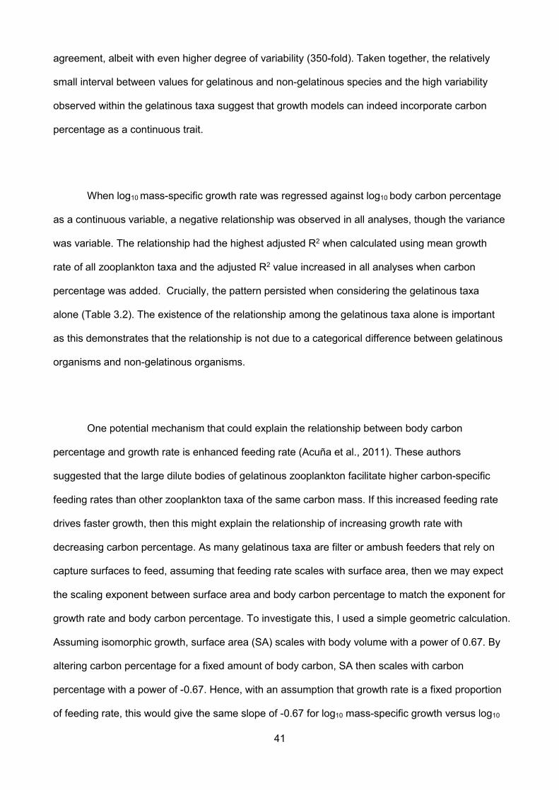
41
agreement, albeit with even higher degree of variability (350-fold). Taken together, the relatively
small interval between values for gelatinous and non-gelatinous species and the high variability
observed within the gelatinous taxa suggest that growth models can indeed incorporate carbon
percentage as a continuous trait.
When log10mass-specific growth rate was regressed against log10 body carbon percentage
as a continuous variable, a negative relationship was observed in all analyses, though the variance
was variable. The relationship had the highest adjusted R2 when calculated using mean growth
rate of all zooplankton taxa and the adjusted R2 value increased in all analyses when carbon
percentage was added. Crucially, the pattern persisted when considering the gelatinous taxa
alone (Table 3.2). The existence of the relationship among the gelatinous taxa alone is important
as this demonstrates that the relationship is not due to a categorical difference between gelatinous
organisms and non-gelatinous organisms.
One potential mechanism that could explain the relationship between body carbon
percentage and growth rate is enhanced feeding rate (Acuña et al., 2011). These authors
suggested that the large dilute bodies of gelatinous zooplankton facilitate higher carbon-specific
feeding rates than other zooplankton taxa of the same carbon mass. If this increased feeding rate
drives faster growth, then this might explain the relationship of increasing growth rate with
decreasing carbon percentage. As many gelatinous taxa are filter or ambush feeders that rely on
capture surfaces to feed, assuming that feeding rate scales with surface area, then we may expect
the scaling exponent between surface area and body carbon percentage to match the exponent for
growth rate and body carbon percentage. To investigate this, I used a simple geometric calculation.
Assuming isomorphic growth, surface area (SA) scales with body volume with a power of 0.67. By
altering carbon percentage for a fixed amount of body carbon, SA then scales with carbon
percentage with a power of -0.67. Hence, with an assumption that growth rate is a fixed proportion
of feeding rate, this would give the same slope of -0.67 for log10 mass-specific growth versus log10
42
carbon percentage (Table 3.1). The exponents that I determined empirically across the various
zooplankton taxa are less steeply negative than -0.67 (at -0.18 and -0.16 for mean and maximum
respectively), i.e. with decreasing carbon percentage, organisms increase their growth rate less
rapidly than these surface considerations would predict. This could indicate a potential feeding
inefficiency associated with decreasing carbon percentage, or that factors additional to surface
area may also be important.
In common with Ikeda (2014), I found that species with larger total carbon masses also
tended to be more watery. Since high carbon masses and water content are both associated with
high growth rates, the effects of carbon mass and carbon percentage tend to counteract,
underscoring the need to include these variables together in order to better predict growth. Molina-
Ramirez et al. (2015) found a similar result for tunicates but found that body carbon percentage
was invariant with increasing mass for cnidarians and ctenophores. The authors suggested that
this might be due to differences between internal filter feeding in tunicates and external ambush or
cruise feeding in the other groups. It has been suggested that feeding modes decrease in
efficiency with increasing volume (Kiørboe et al., 2011), so high water content may help to mitigate
this decrease in efficiency and maintain relatively higher carbon specific feeding rate at large
carbon masses. This assertion is supported by the findings of Acuña et al. (2011), suggesting that
gelatinous plankton had higher carbon-specific feeding rates than other zooplankton of a similar
carbon mass.
While the increase in capture surface area and associated feeding and growth rates is one
potential advantage of the gelatinous body form, there are other implications. There are potential
negative implications such as limited swimming speed and escape responses. While medusae
have potential defences in the form of nematocysts, many gelatinous taxa such as ctenophores
and thaliaceans do not, and may have limited ability to escape from potential predators as a result
of their large dilute bodies (Acuña, et al., 2011). Understanding why some taxa are gelatinous is
43
not always straightforward. The most gelatinous mollusc in this analysis is Clione limacina, a
gymnosome predator that feeds almost exclusively on Limacina helicina. Clione does not rely on
large capture surfaces or on generating a feeding current as it ambushes individual, relatively large
prey items (Lalli and Gilmer, 1989). In this case, low carbon percentage does not appear to be a
derived trait to increase body volume relative to carbon for feeding, suggesting that this may not be
the only driver of low carbon percentage in zooplankton. It has been suggested that potential other
causes include physical or ecological factors such as transparency to impair visual predation
(Hamner et al., 1975) or the efficiency of neutral buoyancy (Kiørboe, 2013). Together these factors
may help to explain why semi-gelatinous bodies are observed in at least six major planktonic phyla
(Cnidaria, Ctenophora, Chordata, Annelida, Chaetognatha, Mollusca, see Appendix I).
The newly established relationship between carbon percentage and growth rate was
applied to improve estimates of secondary production in Figure 3.6. The addition of carbon
percentage to models of secondary production had a significant effect on the outputs. Inclusion of
carbon percentage increased estimates of secondary production at all time points. This was
particularly evident in summer when a range of gelatinous and semi-gelatinous taxa co-occurred
with the crustaceans. The difference between the two estimates was negatively related to carbon
percentage (df = 158, p < 0.0001). This is logical as when the average carbon percentage is lower,
the carbon percentage term will have a greater effect on the estimate and the estimates will differ
further.
To make production estimates including the effects of carbon percentage would normally
require dividing into different groups. For instance, other studies have presented 11 different
growth equations for specific zooplankton groups (Kiørboe and Hirst, 2014). This can be useful for
modelling the growth rate of a specific taxon; however, when attempting to represent the growth of
a full zooplankton assemblage dividing into these constituent groups increases model complexity
and increases uncertainty for important groups poorly served with data, such as siphonophores,
chaetognaths and meroplanktonic larvae. Conversely, if a unified model is used that estimates
44
growth for all zooplankton on the basis of mass alone, the considerable effects of carbon
percentage will be overlooked (Figure 3.6). Adding carbon percentage to the growth model thus
represents a solution; the additional trait information is now relatively easily derivable, and can be
incorporated into a single equation that substantially increases the explanatopry power of growth
rate.
3.6 - Conclusions
Body size is often described as a master-trait, and is frequently used as the sole intrinsic
variable in empirical and simulation models involving zooplankton growth (Moloney and Field, 1991;
Kiørboe and Hirst, 2014; Anderson et al., 2015a). But what do we mean by “body size”? Carbon
mass is often used as the unit for size, but both my meta-analysis and the real assemblage data
show that carbon percentage also varies greatly. It may even vary negatively with carbon mass,
levering an opposing effect on growth. I argue that as carbon mass and carbon percentage are
both intrinsic factors that influence energy budgets, then we should disentangle their separate
effects in a unified growth model. By adding carbon percentage to models of growth based on
carbon mass alone, we substantially increased their explanatory power, with smaller body masses
and lower body carbon percentages leading to higher specific growth rates. Building on the work of
previous publications (Kiørboe, 2013; Pitt et al., 2013; Molina-Ramirez et al., 2015), I provide a
carbon percentage dataset in Appendix I. By using these source data alongside carbon masses,
the maximum growth rate equation in Table 3.1 may then be used as a starting point to estimate
growth rates attainable by zooplankton.
Alongside the “size” based simplifications used for modelling, there has also been an
increase in “trait-based” modelling in which categorical variables or functional groups are allowed
to vary continuously. A purpose of this chapter is to allow carbon percentage also to be used as a
continuous trait; to facilitate its inclusion alongside carbon mass and other traits such as feeding
mode (Litchman, 2013; Andersen et al. 2015a; Hébert et al., 2017). Since I found that growth rate
45
depended on carbon percentage even among the gelatinous taxa alone, I suggest that considering
and modelling carbon percentage as a continuous trait will reveal the ecological and evolutionary
factors that influence the water content of zooplankton.

46
47
CHAPTER 4 – Intraspecific effects of variable carbon
percentage through ontogenetic development:
morphometrics, feeding and growth of Aurelia aurita
ephyrae
48
4.1 - Introduction
Carbon percentage (carbon mass as a percentage of wet mass) can affect the biology of
zooplankton, even within the gelatinous taxa alone (Chapter 3). In Chapter 3, a negative
relationship was found between carbon percentage and growth rate of zooplankton, suggesting
that more gelatinous taxa have higher growth rates (as predicted in Chapter 2). The ecological
implications of this relationship are numerous, as variability in this trait occurs across different
phylogenetic scales. Carbon percentage varies over four orders of magnitude across the
zooplankton as a whole, and congeneric species can differ by as much as an order of magnitude
(Kiørboe, 2013).
Despite this interspecific variability, studies have suggested that there is limited intraspecific
variability in carbon percentage, such that species-specific values are reasonable approximations
(Kiørboe, 2013; Molina-Ramirez et al., 2015). However, these studies focussed almost exclusively
on adult zooplankton, not investigating early ontogeny. Adults of many species of zooplankton are
more ecologically and structurally different from their own larvae than from adults of other species.
For instance, scyphomedusae have a metagenetic life cycle, with separate planktonic sexual
(medusae) and benthic asexual phases (polyp) (Arai, 2012). Polyps are structurally and
ecologically distinct from medusa of the same species, and therefore might also differ in carbon
percentage. During the life cycle of most scyphozoan jellyfish, the polyps strobilate and form larval
jellyfish called ephyrae. As the ephyrae develop they gradually take on the characteristics of the
planktonic medusae stage (Arai, 2012), and therefore are might be expected to change from the
carbon percentage of the polyp to that of the medusa.
This chapter investigated whether ephyrae changed in carbon percentage through
development, and how this change influenced growth and ingestion rates. The interspecific results
in Chapter 3 suggested that taxa with larger bodies tended to be more gelatinous, so it was
predicted that carbon percentage will decrease with increasing diameter as the ephyrae develop. If
49
the range of carbon percentage observed is of a similar magnitude to that of the interspecific study
(0.07 to 0.87%, Chapter 3) then growth rate may be affected.
If a relationship exists between carbon mass and carbon percentage, then demarking
between the effects of these two variables could be difficult. One way to investigate the effects is to
compare the values and exponents with studies on other zooplankton species through
development. Hirst and Forster (2013) found that the intraspecific growth rate (mg C d-1) of many
invertebrates can be described as an exponential relationship with a body mass scaling exponent
of b = 1. If the general growth exponent is approximately 1, then the exponent of the ephyrae is
expected to be greater than this as decreasing carbon percentage is expected to increase growth
rate.
In addition to investigating how variability in carbon percentage through development
affected growth rate, this chapter also aimed to understand how ingestion rate is affected.
Ingestion rate is a key metabolic factor that is expected to be influenced by carbon percentage
(Acuña et al., 2011). This study by Acuña demonstrated that the carbon specific ingestion rate of
gelatinous zooplankton is higher than that of other zooplankton as increased wet mass leads to
higher effective body volumes and therefore higher ingestion rates. However, specific feeding
modes decrease in efficiency with increasing body volume (Kiørboe, 2011). Therefore, I
hypothesised that carbon specific ingestion rates would be similar to comparable zooplankton at
low carbon masses, but would be higher at higher carbon masses. This effect could manifest as
the ephyrae in this chapter having a higher exponent for carbon mass specific ingestion than other
comparable zooplankton.
Taking these points together, carbon percentage was predicted to decrease through
ontogeny in Aurelia aurita ephyrae. This was predicted to increase the scaling exponents of carbon
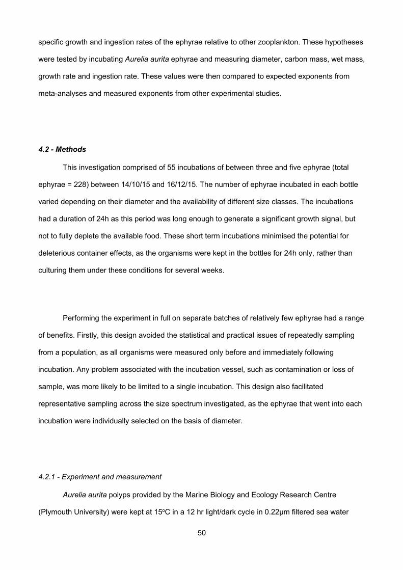
50
specific growth and ingestion rates of the ephyrae relative to other zooplankton. These hypotheses
were tested by incubating Aurelia aurita ephyrae and measuring diameter, carbon mass, wet mass,
growth rate and ingestion rate. These values were then compared to expected exponents from
meta-analyses and measured exponents from other experimental studies.
4.2 - Methods
This investigation comprised of 55 incubations of between three and five ephyrae (total
ephyrae = 228) between 14/10/15 and 16/12/15. The number of ephyrae incubated in each bottle
varied depending on their diameter and the availability of different size classes. The incubations
had a duration of 24h as this period was long enough to generate a significant growth signal, but
not to fully deplete the available food. These short term incubations minimised the potential for
deleterious container effects, as the organisms were kept in the bottles for 24h only, rather than
culturing them under these conditions for several weeks.
Performing the experiment in full on separate batches of relatively few ephyrae had a range
of benefits. Firstly, this design avoided the statistical and practical issues of repeatedly sampling
from a population, as all organisms were measured only before and immediately following
incubation. Any problem associated with the incubation vessel, such as contamination or loss of
sample, was more likely to be limited to a single incubation. This design also facilitated
representative sampling across the size spectrum investigated, as the ephyrae that went into each
incubation were individually selected on the basis of diameter.
4.2.1 - Experiment and measurement
Aurelia aurita polyps provided by the Marine Biology and Ecology Research Centre
(Plymouth University) were kept at 15oC in a 12 hr light/dark cycle in 0.22µm filtered sea water

51
(collected from the L4 sampling site, Chapter 2). Strobilation took place naturally over several
months, with the ephyrae developing in aerated plastic buckets (vol. = 15 l) with full water changes
every two days.
For each experiment, between 22 and 25 ephyrae were selected and photographed under
low magnification (Olympus SZX16, Martin Company MDSLR, Canon EOS 550D, 13x
magnification). The inter-rhophalial diameter (IRD, distance between rhopalia (cnidarian sensory
organs found between the lappet tips) on opposite sides of the animal (Figure 4.1), was obtained
from each image using appropriate computer software (Image J). As all ephyrae were the same
distance from the lens, the number of pixels corresponded to length. A reference picture of a ruler
was taken to convert the values from pixels in mm (IRD varied between 1.2 and 9.1 mm). It was
not possible to match up the identities of the ephyrae before and after the incubation. Therefore, to
get the best possible estimates of individual growth, the ephyrae were ranked based on IRD and
organised into groups of between three and five individuals (depending on diameter). Ephyrae of a
similar diameter were pooled to decrease the standard deviation in diameter of each bottle when
measured after incubation.
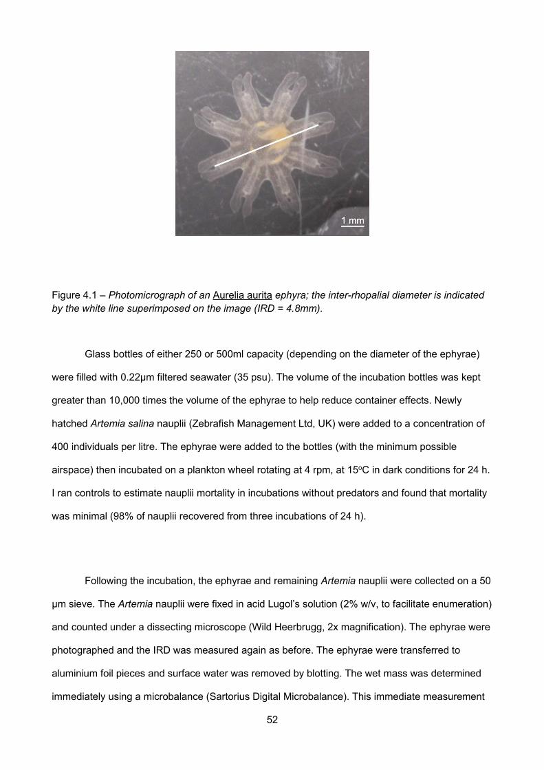
52
Figure 4.1 – Photomicrograph of an Aurelia aurita ephyra; the inter-rhopalial diameter is indicatedby the white line superimposed on the image (IRD = 4.8mm).
Glass bottles of either 250 or 500ml capacity (depending on the diameter of the ephyrae)
were filled with 0.22µm filtered seawater (35 psu). The volume of the incubation bottles was kept
greater than 10,000 times the volume of the ephyrae to help reduce container effects. Newly
hatched Artemia salina nauplii (Zebrafish Management Ltd, UK) were added to a concentration of
400 individuals per litre. The ephyrae were added to the bottles (with the minimum possible
airspace) then incubated on a plankton wheel rotating at 4 rpm, at 15oC in dark conditions for 24 h.
I ran controls to estimate nauplii mortality in incubations without predators and found that mortality
was minimal (98% of nauplii recovered from three incubations of 24 h).
Following the incubation, the ephyrae and remaining Artemia nauplii were collected on a 50
µm sieve. The Artemia nauplii were fixed in acid Lugol’s solution (2% w/v, to facilitate enumeration)
and counted under a dissecting microscope (Wild Heerbrugg, 2x magnification). The ephyrae were
photographed and the IRD was measured again as before. The ephyrae were transferred to
aluminium foil pieces and surface water was removed by blotting. The wet mass was determined
immediately using a microbalance (Sartorius Digital Microbalance). This immediate measurement
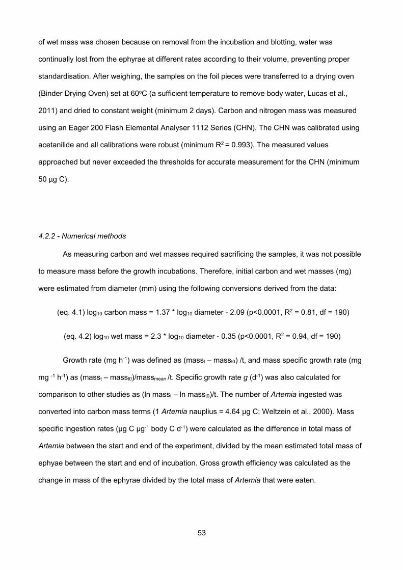
53
of wet mass was chosen because on removal from the incubation and blotting, water was
continually lost from the ephyrae at different rates according to their volume, preventing proper
standardisation. After weighing, the samples on the foil pieces were transferred to a drying oven
(Binder Drying Oven) set at 60oC (a sufficient temperature to remove body water, Lucas et al.,
2011) and dried to constant weight (minimum 2 days). Carbon and nitrogen mass was measured
using an Eager 200 Flash Elemental Analyser 1112 Series (CHN). The CHN was calibrated using
acetanilide and all calibrations were robust (minimum R2= 0.993). The measured values
approached but never exceeded the thresholds for accurate measurement for the CHN (minimum
50 µg C).
4.2.2 - Numerical methods
As measuring carbon and wet masses required sacrificing the samples, it was not possible
to measure mass before the growth incubations. Therefore, initial carbon and wet masses (mg)
were estimated from diameter (mm) using the following conversions derived from the data:
(eq. 4.1) log10 carbon mass = 1.37 * log10 diameter - 2.09 (p<0.0001, R2 = 0.81, df = 190)
(eq. 4.2) log10 wet mass = 2.3 * log10 diameter - 0.35 (p<0.0001, R2 = 0.94, df = 190)
Growth rate (mg h-1) was defined as (masst – masst0) /t, and mass specific growth rate (mg
mg -1 h-1) as (masst – masst0)/massmean /t. Specific growth rate g (d-1) was also calculated for
comparison to other studies as (ln masst – ln masst0)/t. The number of Artemia ingested was
converted into carbon mass terms (1 Artemia nauplius = 4.64 µg C; Weltzein et al., 2000). Mass
specific ingestion rates (µg C µg-1 body C d-1) were calculated as the difference in total mass of
Artemia between the start and end of the experiment, divided by the mean estimated total mass of
ephyae between the start and end of incubation. Gross growth efficiency was calculated as the
change in mass of the ephyrae divided by the total mass of Artemia that were eaten.
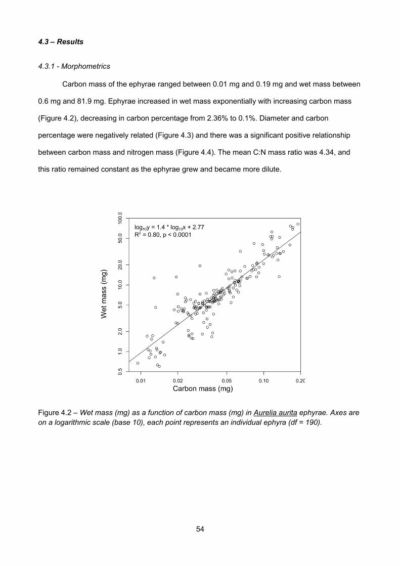
54
4.3 – Results
4.3.1 - Morphometrics
Carbon mass of the ephyrae ranged between 0.01 mg and 0.19 mg and wet mass between
0.6 mg and 81.9 mg. Ephyrae increased in wet mass exponentially with increasing carbon mass
(Figure 4.2), decreasing in carbon percentage from 2.36% to 0.1%. Diameter and carbon
percentage were negatively related (Figure 4.3) and there was a significant positive relationship
between carbon mass and nitrogen mass (Figure 4.4). The mean C:N mass ratio was 4.34, and
this ratio remained constant as the ephyrae grew and became more dilute.
Figure 4.2 – Wet mass (mg) as a function of carbon mass (mg) in Aurelia aurita ephyrae. Axes areon a logarithmic scale (base 10), each point represents an individual ephyra (df = 190).
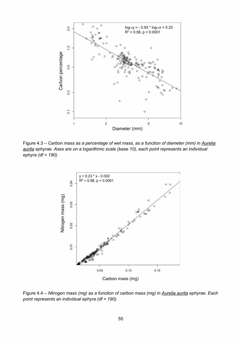
55
Figure 4.3 – Carbon mass as a percentage of wet mass, as a function of diameter (mm) in Aureliaaurita ephyrae. Axes are on a logarithmic scale (base 10), each point represents an individualephyra (df = 190).
Figure 4.4 – Nitrogen mass (mg) as a function of carbon mass (mg) in Aurelia aurita ephyrae. Eachpoint represents an individual ephyra (df = 190).

56
4.3.2 – Ingestion rate
Ingestion rate varied between 4.6 and 91.5 µg C d-1 (Figure 4.5) and was positively related
to diameter (Figure 4.6). The scaling exponent for ingestion rate with increasing carbon mass was
0.6 (Figure 4.5) and with increasing wet mass was 0.33. Ingestion rate decreased with increasing
carbon percentage.
Figure 4.5 – Ingestion rate (µg C ind-1 d-1) of Aurelia aurita ephyrae as a function of carbon mass(mg, log10y = 0.6 * log10x + 2.04, R2 = 0.58, p < 0.0001), wet mass (mg, log10y = 0.33 * log10x –2.07, R2 = 0.4, p < 0.0001) and carbon percentage (log10y = - 0.35 * log10x + 1.12, R2 = 0.07, p =0.047). Axes are on a logarithmic scale (base 10), each point represents an individual ephyra (df =41).
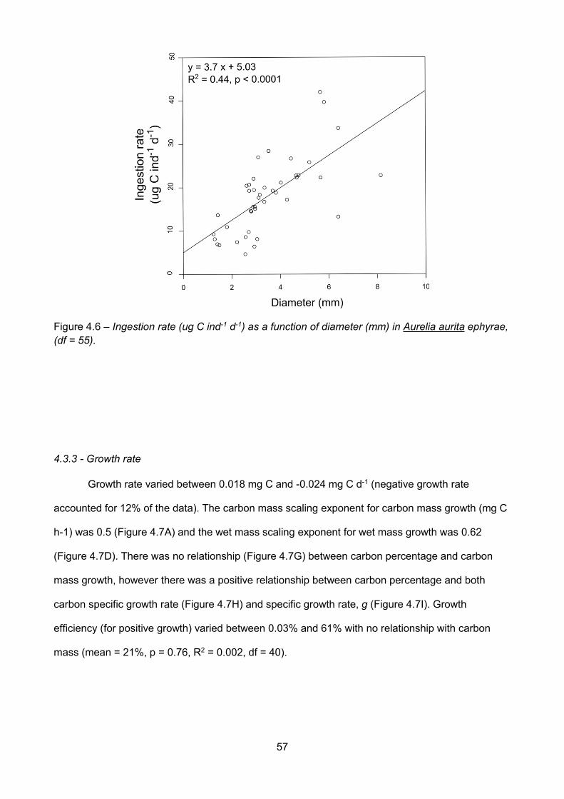
57
Figure 4.6 – Ingestion rate (ug C ind-1 d-1) as a function of diameter (mm) in Aurelia aurita ephyrae,(df = 55).
4.3.3 - Growth rate
Growth rate varied between 0.018 mg C and -0.024 mg C d-1 (negative growth rate
accounted for 12% of the data). The carbon mass scaling exponent for carbon mass growth (mg C
h-1) was 0.5 (Figure 4.7A) and the wet mass scaling exponent for wet mass growth was 0.62
(Figure 4.7D). There was no relationship (Figure 4.7G) between carbon percentage and carbon
mass growth, however there was a positive relationship between carbon percentage and both
carbon specific growth rate (Figure 4.7H) and specific growth rate, g (Figure 4.7I). Growth
efficiency (for positive growth) varied between 0.03% and 61% with no relationship with carbon
mass (mean = 21%, p = 0.76, R2 = 0.002, df = 40).
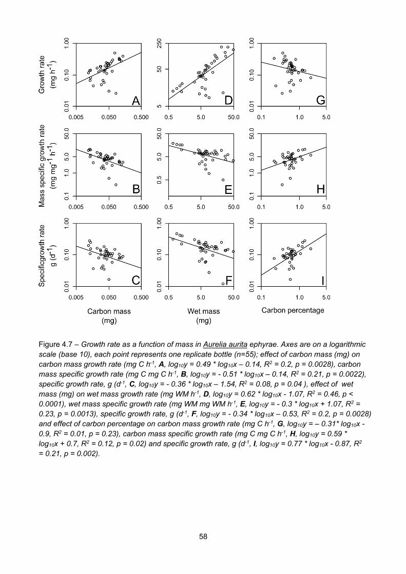
58
Figure 4.7 – Growth rate as a function of mass in Aurelia aurita ephyrae. Axes are on a logarithmicscale (base 10), each point represents one replicate bottle (n=55); effect of carbon mass (mg) oncarbon mass growth rate (mg C h-1, A, log10y = 0.49 * log10x – 0.14, R2 = 0.2, p = 0.0028), carbonmass specific growth rate (mg C mg C h-1, B, log10y = - 0.51 * log10x – 0.14, R2 = 0.21, p = 0.0022),specific growth rate, g (d-1, C, log10y = - 0.36 * log10x – 1.54, R2 = 0.08, p = 0.04 ), effect of wetmass (mg) on wet mass growth rate (mg WM h-1, D, log10y = 0.62 * log10x - 1.07, R2 = 0.46, p <0.0001), wet mass specific growth rate (mg WM mg WM h-1, E, log10y = - 0.3 * log10x + 1.07, R2 =0.23, p = 0.0013), specific growth rate, g (d-1, F, log10y = - 0.34 * log10x – 0.53, R2 = 0.2, p = 0.0028)and effect of carbon percentage on carbon mass growth rate (mg C h-1, G, log10y = – 0.31* log10x -0.9, R2 = 0.01, p = 0.23), carbon mass specific growth rate (mg C mg C h-1, H, log10y = 0.59 *log10x + 0.7, R2 = 0.12, p = 0.02) and specific growth rate, g (d-1, I, log10y = 0.77 * log10x - 0.87, R2
= 0.21, p = 0.002).
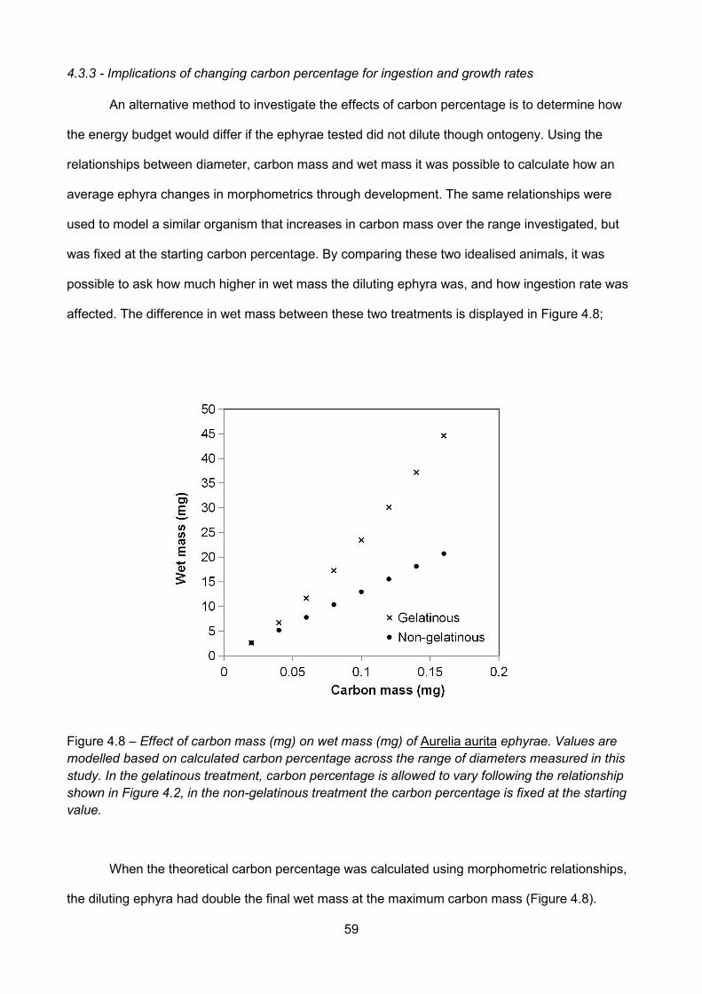
59
4.3.3 - Implications of changing carbon percentage for ingestion and growth rates
An alternative method to investigate the effects of carbon percentage is to determine how
the energy budget would differ if the ephyrae tested did not dilute though ontogeny. Using the
relationships between diameter, carbon mass and wet mass it was possible to calculate how an
average ephyra changes in morphometrics through development. The same relationships were
used to model a similar organism that increases in carbon mass over the range investigated, but
was fixed at the starting carbon percentage. By comparing these two idealised animals, it was
possible to ask how much higher in wet mass the diluting ephyra was, and how ingestion rate was
affected. The difference in wet mass between these two treatments is displayed in Figure 4.8;
Figure 4.8 – Effect of carbon mass (mg) on wet mass (mg) of Aurelia aurita ephyrae. Values aremodelled based on calculated carbon percentage across the range of diameters measured in thisstudy. In the gelatinous treatment, carbon percentage is allowed to vary following the relationshipshown in Figure 4.2, in the non-gelatinous treatment the carbon percentage is fixed at the startingvalue.
When the theoretical carbon percentage was calculated using morphometric relationships,
the diluting ephyra had double the final wet mass at the maximum carbon mass (Figure 4.8).
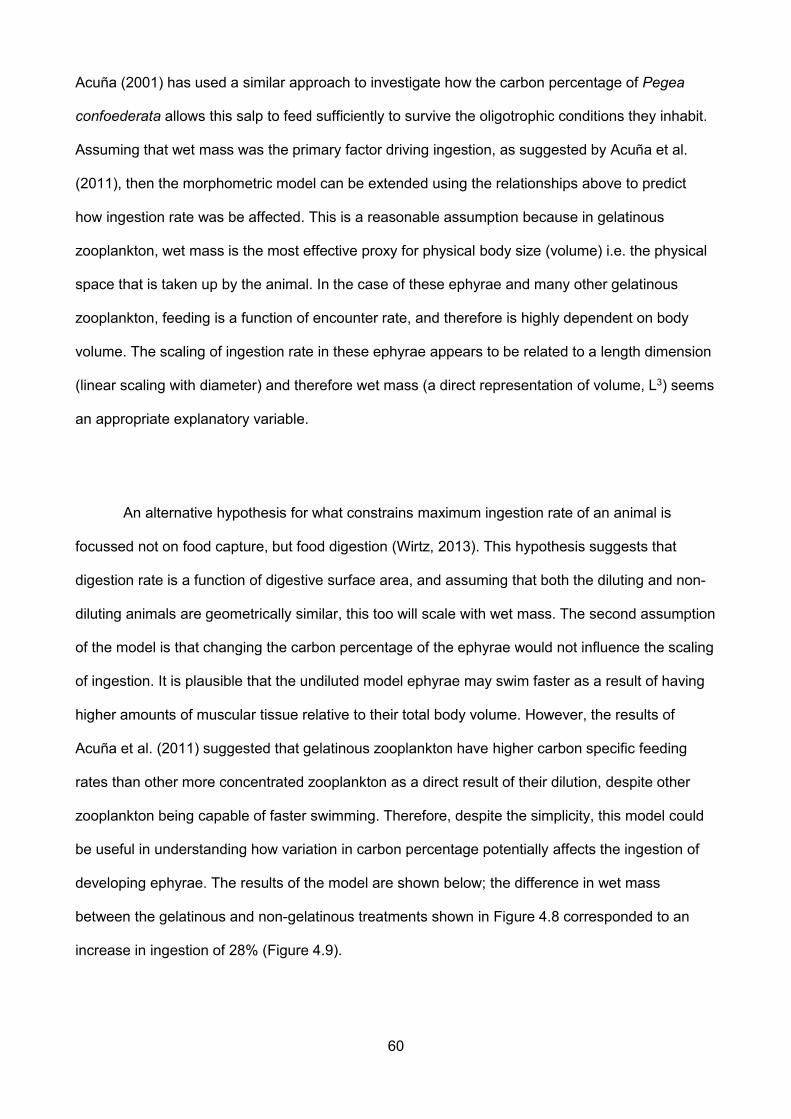
60
Acuña (2001) has used a similar approach to investigate how the carbon percentage of Pegea
confoederata allows this salp to feed sufficiently to survive the oligotrophic conditions they inhabit.
Assuming that wet mass was the primary factor driving ingestion, as suggested by Acuña et al.
(2011), then the morphometric model can be extended using the relationships above to predict
how ingestion rate was be affected. This is a reasonable assumption because in gelatinous
zooplankton, wet mass is the most effective proxy for physical body size (volume) i.e. the physical
space that is taken up by the animal. In the case of these ephyrae and many other gelatinous
zooplankton, feeding is a function of encounter rate, and therefore is highly dependent on body
volume. The scaling of ingestion rate in these ephyrae appears to be related to a length dimension
(linear scaling with diameter) and therefore wet mass (a direct representation of volume, L3) seems
an appropriate explanatory variable.
An alternative hypothesis for what constrains maximum ingestion rate of an animal is
focussed not on food capture, but food digestion (Wirtz, 2013). This hypothesis suggests that
digestion rate is a function of digestive surface area, and assuming that both the diluting and non-
diluting animals are geometrically similar, this too will scale with wet mass. The second assumption
of the model is that changing the carbon percentage of the ephyrae would not influence the scaling
of ingestion. It is plausible that the undiluted model ephyrae may swim faster as a result of having
higher amounts of muscular tissue relative to their total body volume. However, the results of
Acuña et al. (2011) suggested that gelatinous zooplankton have higher carbon specific feeding
rates than other more concentrated zooplankton as a direct result of their dilution, despite other
zooplankton being capable of faster swimming. Therefore, despite the simplicity, this model could
be useful in understanding how variation in carbon percentage potentially affects the ingestion of
developing ephyrae. The results of the model are shown below; the difference in wet mass
between the gelatinous and non-gelatinous treatments shown in Figure 4.8 corresponded to an
increase in ingestion of 28% (Figure 4.9).
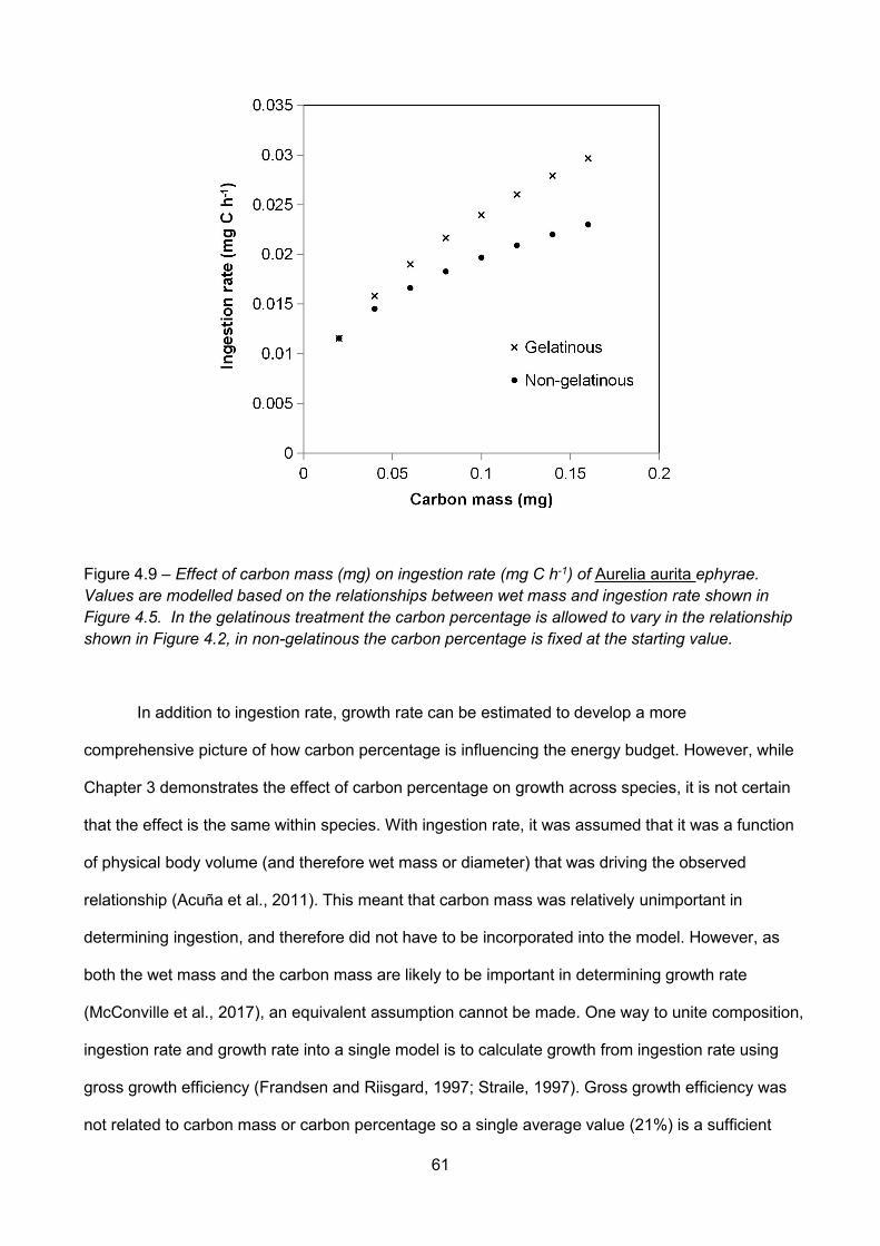
61
Figure 4.9 – Effect of carbon mass (mg) on ingestion rate (mg C h-1) of Aurelia aurita ephyrae.Values are modelled based on the relationships between wet mass and ingestion rate shown inFigure 4.5. In the gelatinous treatment the carbon percentage is allowed to vary in the relationshipshown in Figure 4.2, in non-gelatinous the carbon percentage is fixed at the starting value.
In addition to ingestion rate, growth rate can be estimated to develop a more
comprehensive picture of how carbon percentage is influencing the energy budget. However, while
Chapter 3 demonstrates the effect of carbon percentage on growth across species, it is not certain
that the effect is the same within species. With ingestion rate, it was assumed that it was a function
of physical body volume (and therefore wet mass or diameter) that was driving the observed
relationship (Acuña et al., 2011). This meant that carbon mass was relatively unimportant in
determining ingestion, and therefore did not have to be incorporated into the model. However, as
both the wet mass and the carbon mass are likely to be important in determining growth rate
(McConville et al., 2017), an equivalent assumption cannot be made. One way to unite composition,
ingestion rate and growth rate into a single model is to calculate growth from ingestion rate using
gross growth efficiency (Frandsen and Riisgard, 1997; Straile, 1997). Gross growth efficiency was
not related to carbon mass or carbon percentage so a single average value (21%) is a sufficient
62
approximation. Taking GGE to be a constant value means that growth can be estimated based on
ingestion alone, and the model can estimate the carbon or wet mass of the two treatments over
time. Figure 4.10 shows that when the change in wet mass over time is estimated, the gelatinous
treatment reaches a disproportionately higher wet mass than would be expected based on Figure
4.8 alone. This is a result of the positive feedback interaction between progressive dilution and
ingestion rate, the dilution of the gelatinous treatment leads to higher feeding rates, which in turn
leads to faster growth rate. As a result of this positive feedback, the model quickly becomes
unrealistic beyond the range of the data observed in our experiment. In reality, the relationship
seen above could not continue past the range shown as carbon percentage of Aurelia aurita does
not dilute indefinitely, but to a minimum carbon percentage of 0.1% (Kiørboe, 2013).
Figure 4.10 – Growth in terms of daily change in wet mass (mg) of Aurelia aurita ephyrae. Valuesare modelled based on the relationships between wet mass and ingestion rate observed in ourdata. In the gelatinous treatment, carbon percentage is allowed to vary in the relationshipobserved in our data, in non-gelatinous the carbon percentage is fixed at the starting value.

63
Using the model shown in Figure 4.10, it is possible to calculate what the mass scaling
exponent for growth would be if dilution only influenced growth rate through increasing ingestion
rate. The exponent for the specific growth rate, g (d-1), generated from the model is 0.39, which is
similar to the exponent derived from measured growth rates shown above (0.36, Figure 4.7C). This
value is the result of the interaction between dilution and ingestion rate alone so it is surprising that
it is so similar to the measured exponent. This could suggest that the exponent observed for
growth rate in the experimental study is primarily determined by limitations in maximum possible
feeding rate. This could be a consequence of sub-optimal food quality, as Moller and Riisgard
(2007) found that Aurelia aurita ephyrae were capable of growing more quickly when offered the
hydromedusae, Rathkea octopunctata (even with lower prey carbon mass). The model also implies
that as the ephyrae grow and decrease in carbon percentage, feeding rate increases as growth
efficiency remains constant, leading to proportionally higher growth. Therefore wet mass would
increase exponentially through time until the adult carbon percentage was reached. This is
ecologically relevant as predation mortality in zooplankton is often related to length along the major
axis, or wet mass. Mortality due to predation is a major factor in determining recruitment of larval
zooplankton (Platt, 1985), therefore minimising the time spent at a relatively small body size can
lead to increased adult abundance. Through dilution, ephyrae grow through this vulnerable size
range faster than other zooplankton, potentially decreasing mortality.
4.4 - Discussion
This chapter is the first study, to my knowledge, to investigate the effects of intraspecific
variation in carbon percentage on the energy budget of zooplankton, although other studies have
taken growth and ingestion measurements of Aurelia aurita ephyrae (Olesen et al., 1994; Hannson,
1997; Bamstedt et al., 2001). The most directly comparable study is that of Møller and Riisgard
(2007) on Aurelia aurita, Sarsia tubulosa and Aequorea vitrina. In common with this chapter, Møller
and Riisgard (2007) measured the specific growth rate and ingestion rate of Aurelia aurita ephyrae
feeding on Artemia nauplii. As the food provided and ephyrae size range of Møller and Riisgard
64
(2007) is similar to those of this chapter, their study provide a valuable comparison with my
measurements.
The smallest epyhrae had carbon percentage of 2.3% and diluted through development to
the adult value of 0.1%. The newly strobilated ephyrae differed in carbon percentage from both
adult Aurelia aurita and the mean carbon percentage of gelatinous zooplankton as a whole (~0.5%,
Kiørboe, 2011). The smallest ephyrae were closer to the carbon percentage of chaetognaths and
other intermediately gelatinous zooplankton than other cnidarians (Kiørboe, 2013). This suggests
that the early developmental stages of gelatinous taxa represent a group of intermediately
gelatinous zooplankton that may not have been previously appreciated. In the study by Kiørboe
(2013) it was suggested that there are relatively few taxa of intermediate carbon percentage.
However, if at least some gelatinous taxa dilute through development, then a far greater number of
taxa are of intermediate carbon percentage at some point in their ontogeny. Gelatinous
zooplankton are routinely under-sampled with nets, due to their delicacy and difficulty of
identification (Raskoff et al., 2003) and larval animals are often more numerous than adults of the
same species (Cross et al., 2015). Taken together, this could suggest that a substantial fraction of
some zooplankton assemblages are of intermediate carbon percentage. In addition, the range of
carbon percentage observed also suggests that it is unreliable to use taxon-specific averages for
carbon percentage of early life stages of Aurelia aurita, and potentially other scyphomedusae.
The C:N mass ratio did not change with ontogeny (mean = 4.34) across all body sizes
suggesting that all somatic carbon was metabolically active, not being stored as lipid (Schmidt et
al., 2003). This value is similar to other non-lipid storing zooplankton (Ikeda and Takahashi, 2012;
Ikeda, 2013) and to other gelatinous zooplankton (Ikeda, 2014). This value is lower than the
Redfield ratio (Redfield, 1934), as expected for an obligate carnivore. The C:N ratio for Artemia
nauplii is approximately 3.65, lower than that of the ephyrae but is likely similar enough for
adequate nutrition (based on the fixed C:N of the ephyrae through development).
65
4.4.1 - Ingestion
For an ephyra of 16.8 µg C feeding on Artemia nauplii, this chapter reported an ingestion
rate of 9.5 µg C d-1, compared to 20.2 µg C d-1 reported in Møller and Riisgard (2007). The values
observed were also lower than the ingestion rates reported for Calanus helgolandicus over a range
of carbon masses (Harris et al., 2007). The ephyrae fed at lower rates than other comparable
zooplankton, despite being offered high concentrations of food at the same temperature (400 µg C
l-1 in this study relative to 280 µg C l-1 in Harris et al., 2007). This could suggest that the incubation
vessels were deleterious to ephyra condition. There was however, limited support for deleterious
tank effects as mortality was low (mortality rate = 1.3%) and behaviour was not significantly
different post-incubation. It is unclear why the ephyrae fed at lower rates than other comparable
zooplankton, as previous studies have suggested that decreased carbon percentage increases
carbon specific feeding rate (Acuña et al., 2011).
With increasing mass, specific feeding modes are expected to become less efficient
(Kiørboe, 2011), resulting in intraspecific ingestion rates to scaling at b < 1. Ingestion rate
increased with increasing carbon mass, with a scaling exponent of 0.6 with increasing carbon
mass (Figure 4.5), and 0.33 with increasing wet mass (Figure 4.5). The carbon mass scaling
exponent of the ephyrae is very similar to that of C. helgolandicus (0.59, Harris et al., 2007). This
was unexpected as the dilution of the ephyrae was predicted to increase the ingestion rate
exponent with increasing carbon mass. As carbon mass increased, wet mass increased
disproportionately (Figure 4.2). As ingestion rate is a function of wet mass (Acuña et al., 2011), it
was expected that this dilution would increase the carbon mass scaling exponent of the ephyrae
relative to the non-diluting C. helgolandicus. As the exponent was similar, either the intraspecific
variation in carbon percentage was insufficient to reproduce the interspecific pattern identified by
Acuña et al. (2011), or other factors are more important in determining the ingestion rate of
ephyrae.
66
In addition, the wet mass scaling exponent was also lower than predicted. As C.
heloglandicus does not have a gelatinous body form, it is assumed that carbon percentage
remains relatively constant through development, therefore the wet mass scaling exponent for
ingestion for C. helgolandicus should be equal to the carbon mass scaling exponent (0.59). The
exponent of 0.33 observed for the ephyrae is lower than the exponent for C. helgolandicus (0.59),
which could suggest that tissue dilution has a negative effect on feeding. However, there is an
alternative hypothesis as the specific value of the exponent (b = 0.33) suggests that feeding may
be a function of a length dimension, and not a function of wet mass (b = 1) or surface area (b =
0.67). In a study on ephyra prey capture mechanics, Sullivan et al. (1997) reported that 61% of
captures took place on the lappet tips. If prey capture is much more likely on the lappet tips than
other areas of the ephyrae, then it would follow that ingestion rate would increase at a rate similar
to the rate at which the lappet tip area increases (potentially due to nematocyst distribution or flow
regime). The lappet tips are the outermost areas of each lappet, and therefore are a proportion of
the circumference. As the lappet tips constitute a proportion of the circumference of the ephyra,
they are a length dimensions, and could be expected to scale at approximately b = 0.33 with wet
mass. If this is the case, ingestion rate is expected to increase linearly with increasing diameter, as
seen in Figure 4.6.
There was a negative relationship between carbon percentage and ingestion rate. I believe
this was driven by low carbon percentage individuals being much larger (in both carbon and wet
mass terms) and therefore having higher gross ingestion rates. This is also reflected in the
relationship between carbon percentage and specific ingestion rate (log10y = 0.56 * log10x + 2.73,
R2 = 0.33, p < 0.0001), as the relatively low carbon mass of high carbon percentage ephyrae led to
high specific ingestion rates. In this instance, the strong relationship between carbon mass and
carbon percentage (shown by proxy in Figure 4.3) render carbon percentage uninformative.
67
4.4.2 - Growth
Maximum specific growth rate, g (d-1), was 0.28, comparable but higher than the values
reported by Møller and Riisgard (2007) of 0.22 and Olesen et al. (1994) of 0.2. This is likely a result
of using smaller ephyrae in our experiments than the above authors (1.2 mm compared to 3.5 mm
and 4 mm respectively), as the highest g value in this chapter was observed for the smallest
ephyrae. The growth rates of Aurelia aurita ephyrae in this study (g = 0.12) are lower than those of
C. helgolandicus of similar carbon mass (g = 0.20, Harris et al., 2007). This suggests that during
early development of gelatinous zooplankton, carbon percentage may not be as important as other
factors in determining growth rate.
A meta-analysis by Hirst and Forster (2013) on the growth scaling of a wide range of
marine invertebrates suggested that growth rate (mg C d-1) scales most commonly at or
approaching b = 1 within species. Following this, I hypothesised that the growth exponents
observed would be greater than other zooplankton species, as in my interspecific study in Chapter
2, decreasing carbon percentage led to an increase in growth rate. As increasing carbon mass led
to decreasing carbon percentage, I predicted growth rate would increase with increasing carbon
mass, and therefore expected the carbon mass scaling exponent to be greater than 1. The scaling
exponent for wet mass growth rate (mg WM d-1) was 0.62 and for carbon mass growth rate (mg
CM d-1) was 0.49, both lower than predicted. If the ephyrae were reaching maximum adult body
size at the upper range of diameter then this exponent might be expected, however this was not
the case. An alternative hypothesis for a low growth body mass scaling exponent is that the
ephyrae were becoming food limited. Møller and Riisgard (2007) found that with increasing food
concentration, ephyrae grew faster to a maximum rate at 100ug C l-1. Prior to the experiment, the
ephyrae were fed regularly and during the incubations I provided a food concentration considerably
greater than this (460 µg C l-1) minimising the chance that growth was food limited. The low
exponents could suggest that tissue dilution has an associated energetic cost, such that diluting
tissues diverts energy away from increasing in carbon mass. The relationship between carbon
percentage and growth rates mirrors that of carbon percentage and ingestion rate. Carbon mass is
68
the cause of these relationships, as at high carbon percentages, growth rate (mg h-1) is low and
specific growth rate (both mg mg-1 h-1 and g d-1) are low. As with ingestion, the relationship
between carbon mass and carbon percentage means that, in this experiment, carbon percentage
provided limited information about growth.
The mean value for gross growth efficiency (ingestion/growth, GGE = 0.21) observed lies
within the range reported by Straile (1997) for a wide range of other zooplankton. This value was
also comparable to the net growth efficiencies (NGE) reported for ephyrae by Olesen et al. (1994)
0.35 and Frandsen and Riisgard (1997) of 0.37. As the NGE values from the other authors are
based on the proportion of assimilated carbon these values are expected to be higher than the
gross growth efficiency reported in this study, which is calculated from ingested carbon. Previous
studies on other gelatinous zooplankton have observed that gross growth efficiency (GGE) can
decrease or remain constant with increasing length or mass (Kremer and Reeve, 1989; Sullivan
and Gifford, 2007). It is unclear whether the lobate ctenophores in their studies were diluting over
the course of the above investigations, and whether this influenced their GGE. In my study, gross
efficiency was invariant with increasing carbon mass, despite progressive dilution. Above, it was
suggested that the low exponents for growth rate could be due to the costs of dilution. However,
there was no evidence for a relationship between wet mass and gross growth efficiency. This
suggests that the ratio between food ingested and carbon mass increase was constant, despite
wet mass increasing proportionately more in larger ephyrae. While not definitive, this could suggest
that the costs of tissue dilution are minimal and that the low exponents have some other cause.
4.5 - Conclusion
This chapter has demonstrated that carbon percentage is not fixed during the development
of Aurelia aurita.While adult A. aurita have similar carbon percentage values to those of many
other gelatinous taxa, larval ephyrae are more similar to that of chaetognaths or some tunicates.
Carbon percentage was found to vary continuously across the size range investigated, showing a
69
gradual decrease from the ephyrae to the adult value. This lends further support to the notion of
substituting the current categorical view of gelatinous and non-gelatinous zooplankton with a
continuous view based expressed as carbon percentage. Given the absence of data for other
species, it is currently unclear whether this represents a general trend, and whether other
gelatinous taxa also dilute through development. If so, these larvae could constitute a considerable
fraction of the zooplankton that is intermediately gelatinous and not often sampled or considered.
This chapter suggests that biologically relevant variation in carbon percentage does occur
across ontogeny. Ingestion and growth rates in both carbon and wet mass were observed to scale
at lower exponents than those expected from general theory and observed in other zooplankton. It
is difficult to determine whether this is the result of dilution occurring in parallel with growth, and it
is possible that the scaling of growth rate may have a different exponent once the adult carbon
percentage is reached.
In the simple model presented, dilution of the magnitude observed in this chapter lead to an
increase in carbon specific feeding rate of 28% over a similar non-diluting organism. However, this
is uncertain as this difference was not found when comparing with other organisms. The interacting
effects of dilution and ingestion rate on growth suggest that through dilution ephyrae may escape
vulnerable body size classes faster than would be possible through carbon mass growth alone.
Taken in concert, these observations suggest that intraspecific variation in carbon percentage
could have functional implications and demonstrate potential evolutionary drivers for this rapid
dilution in early ontogeny.

70

71
CHAPTER 5 – The influence of carbon percentage on
bloom formation
72
5.1 - Introduction
Recent years have seen a resurgence in the study of phenology, the seasonal timing of
biological events (Edwards and Richardson, 2004; Yang and Rudolf, 2010; Anderson et al., 2012),
partially as a result of concerns over anthropogenic climate change. These changes in timing have
the potential to affect ecosystems in a number of ways, including premature spawning relative to
the timing of suitable foods (Mackas et al., 2012) and trophic mismatching (Beaugrand et al., 2003;
Atkinson et al., 2015). In order to better predict how biological communities will respond to these
changes in seasonal timing, it is important to first establish a robust understanding, terminology
and definition for seasonally recurring phenomena.
One term that is frequently used when discuss timing and seasonality in plankton
communities is “bloom”. Despite its common use, the specific meaning of the word bloom is
ambiguous. For instance, the term bloom is applied to the flowering of angiosperms and rapid
population increase of different groups within the zooplankton. Furthermore, within different
scientific communities, the term bloom is defined differently. Even within the relatively narrow field
of gelatinous zooplankton, some ambiguity remains. An important division made by Graham et al.
(2001) between true and apparent blooms, was later expanded by Lucas and Dawson (2014) into
the definition below;
“A true bloom is in part a consequence of seasonal life cycles, and consequently all metagenicorganisms have the potential to bloom pending suitable environmental conditions; thus normaland/or abnormal seasonal biomass is directly attributable to population increase due toreproduction and growth, sometimes enhanced by anthropogenic activity. An apparent bloom, incontrast, is a local increase in biomass of animals associated with temporary or transient chemicalor physical phenomena (such as aggregation at fronts or local advection to a new location) orlonger term accumulation of large numbers in enclosed habitats; apparent blooms may, but do notnecessarily reflect true blooms that occurred elsewhere” (Lucas and Dawson, 2014)”
Following this definition, the one of the criterion determining whether a transient population
is a bloom is whether the species has a metagenic life cycle (undergoes an alteration of
generations between different phases in the life cycle). Such a definition is incomplete as many
gelatinous taxa that do not have metagenic lifecycles do form blooms. These include the
holoplanktonic medusa, Pelagia noctiluca (Hamner and Dawson, 2008) and the lobate ctenophore,
73
Mnemiopsis leidyi (Fuentes et al., 2010). The opposite is also true. Not all metagenic taxa form
blooms, as documented in the Stauromedusae by Miranda et al. (2012). This demonstrates the
limitations of a definition of blooming based on the intrinsic qualities of the organisms it comprises.
This loose definition of blooming in gelatinous zooplankton contrasts with that used for
phytoplankton blooms, where proxies of abundance (measurements of ocean colour and other
remotely sensed data) are used to produce quantitative definitions. A population is considered to
be blooming when chlorophyll a concentration (as a proxy for biomass) is greater than an
established threshold (Racault et al., 2012). This form of definition is based on the population
dynamics of the taxa, not on an intrinsic quality of their biology. This approach is valuable as
specific aspects of blooming, such as global incidence and duration, can be quantified through the
use of numerical indices. These indices can in turn be used to ask meaningful questions of the
biology of the system, such as to how light and climatic indices influence the phenology and other
large scale patterns of bloom formation (Racault et al., 2012).
The extra information afforded by using a quantitative definition based on indices of
blooming in phytoplankton suggests that applying a similar approach to blooming in zooplankton
could further our understanding. Bloom indices for zooplankton could be valuable in a range of
different ways. For ecologists, quantitative indices for the magnitude of blooms would allow for
descriptive comparisons of blooms in different groups, or trends in blooming in a particular species
over time. Furthermore, the effects of differing degrees of blooming on food web interactions or the
productivity of an area could be investigated, leading to a deeper understanding of how blooming
impacts zooplankton systems.
Blooms of gelatinous zooplankton are also of interest to policy makers, as gelatinous
zooplankton form one of the plankton lifeform indicators as part of the Marine Strategy Framework
74
Directive (MSFD) (Tett et al., 2015). In most cases, the negative interactions between gelatinous
zooplankton and humans occur primarily during blooms (Masalimoni et al, 2000), therefore
monitoring of the blooming of gelatinous zooplankton is of key importance. The creation of
numerical bloom indices could provide further information to policy makers on whether
management strategies are working effectively, on the progress of biological invasions (e.g. is a
population of an invasive species actively blooming?).
The development of quantitative bloom indices could also be useful for asking more
fundamental questions about the relationship between the gelatinous body form and blooming.
Many gelatinous zooplankton form blooms, such as Pelagia notiluca, however some do not, such
as the Stauromedusae. A range of factors contribute to bloom-like dynamics in the zooplankton
including benthic processes, such as strobilation in scyphomedusae (Uye et al., 2006), some of
which are of key importance to the populations of non-gelatinous taxa also. Despite this, the term
bloom is applied exclusively to zooplankton that are gelatinous. One aim of this study is to
investigate whether the population dynamics of gelatinous zooplankton differ quantitatively from
those of other zooplankton, and whether other taxa also form blooms. As the gelatinous
zooplankton are highly diverse in phylogeny, life history and functional ecology, the shared trait to
determine whether an organism should be included within the group is a dilute body. With this is
mind, by relating the bloom indices to carbon percentage for different species, it is possible to test
whether the population dynamics of gelatinous zooplankton differ from those of other zooplankton.
Using these relationships, it is possible to ask whether only gelatinous zooplankton form blooms, or
whether this phenomenon is more widely distributed.

75
The aim of this chapter was to develop a number of indices to define blooms and determine
whether bloom formation is related to carbon percentage. The aim was completed through the
following objectives; first, to consider the population dynamics that may be characteristic of
blooming; second, to suggest ways to capture these characteristics numerically; third, to use
known bloom forming and more stable taxa to evaluate the indices; and fourth to relate the indices
to carbon percentage and carbon mass to test whether more gelatinous taxa are more predisposed
to form blooms.
5.2 - Methods
5.2.1 - Data sources
The data used in this chapter come from the L4 time series, described in detail in Chapter 2.
Taxonomic resolution of identification was increased in 2009, particularly for the hydromedusae,
and therefore only data from 2009-2015 inclusive were used in this analysis (319 time points, 638
net samples). Of the 188 taxa currently recorded, only those that had been consistently recorded
since 2009 were included (127 taxa). Eggs were not included in the analysis.
5.2.2 - Development of bloom indices
Several qualities that are associated with blooming can be visualised by comparing
changes in abundance over time for the two species, A and B, shown in Figure 5.1. Both species
have the same total abundance over the period shown, although the population dynamics of the
species differ. Species A would be described as more bloom-forming than species B, and below
this quality is explored numerically. As this stage there is no attempt to classify the model species
are gelatinous or otherwise, only to identify what numerical qualities are indicative of bloom
formation. Many metagenic gelatinous zooplankton may fit the model of species B more closely as
a result of continuous, or protracted, strobilation through the year (Houghton et al., 2007).
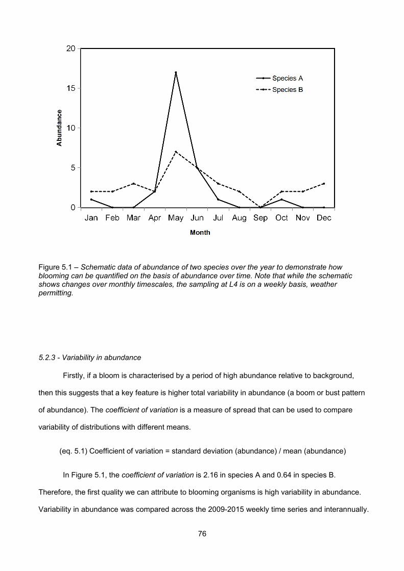
76
Figure 5.1 – Schematic data of abundance of two species over the year to demonstrate howblooming can be quantified on the basis of abundance over time. Note that while the schematicshows changes over monthly timescales, the sampling at L4 is on a weekly basis, weatherpermitting.
5.2.3 - Variability in abundance
Firstly, if a bloom is characterised by a period of high abundance relative to background,
then this suggests that a key feature is higher total variability in abundance (a boom or bust pattern
of abundance). The coefficient of variation is a measure of spread that can be used to compare
variability of distributions with different means.
(eq. 5.1) Coefficient of variation = standard deviation (abundance) / mean (abundance)
In Figure 5.1, the coefficient of variation is 2.16 in species A and 0.64 in species B.
Therefore, the first quality we can attribute to blooming organisms is high variability in abundance.
Variability in abundance was compared across the 2009-2015 weekly time series and interannually.

77
To investigate variability across the time series the coefficient of variation of abundance was
calculated for each species. Two indices were used to estimate interannual variability; the ratio
between the maximum and minimum mean annual abundance, and the coefficient of variation of
mean annual abundances. These indices were calculated including and excluding zeroes, as the
large number of zeroes associated with species presence records tended to strongly decrease
variability in rare species. Species that have more bloom-like population dynamics will have higher
coefficients. If taxa with low carbon percentage have more bloom-like population dynamics then
carbon percentage will be negatively related to; i) coefficient of variation, ii) ratio between the
maximum and minimum mean annual abundances and iii) coefficient of variation of mean annual
abundances.
5.2.4 - Temporal heterogeneity
Furthermore, the relatively high abundances that comprise blooms often increase and
decrease rapidly; so species abundance tends to be concentrated into relatively short periods. In
Figure 5.1, 65% of the total abundance of species A is concentrated in the maximum measurement
compared to 27% in species B. Therefore, temporal heterogeneity in abundance, i.e. long periods
of low (to zero) background abundance punctuated with short periods of high abundance is
another quality associated with blooming.
Temporal heterogeneity could be considered as synonymous with temporal auto-correlation,
the probability of the abundance at sample n+1 being similar to the abundance at sample n.
However, given the patchy distribution and potential aggregation of some plankton species,
random fluctuations that do not represent meaningful increases are common. For this reason, a
temporal auto correlation function was not used as an index. Instead, temporal heterogeneity was
investigated using two indices, the number of non-zero records and the coefficient of the frequency
distribution of abundance.
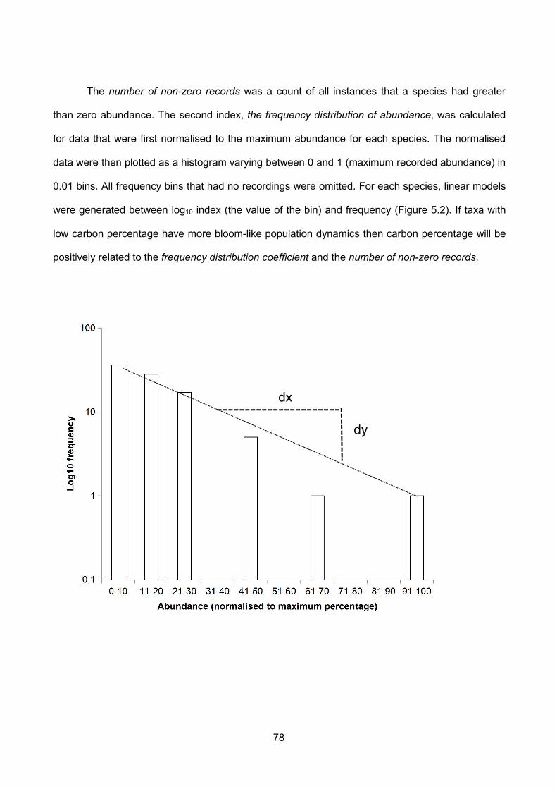
78
The number of non-zero records was a count of all instances that a species had greater
than zero abundance. The second index, the frequency distribution of abundance, was calculated
for data that were first normalised to the maximum abundance for each species. The normalised
data were then plotted as a histogram varying between 0 and 1 (maximum recorded abundance) in
0.01 bins. All frequency bins that had no recordings were omitted. For each species, linear models
were generated between log10 index (the value of the bin) and frequency (Figure 5.2). If taxa with
low carbon percentage have more bloom-like population dynamics then carbon percentage will be
positively related to the frequency distribution coefficient and the number of non-zero records.
dy
dx
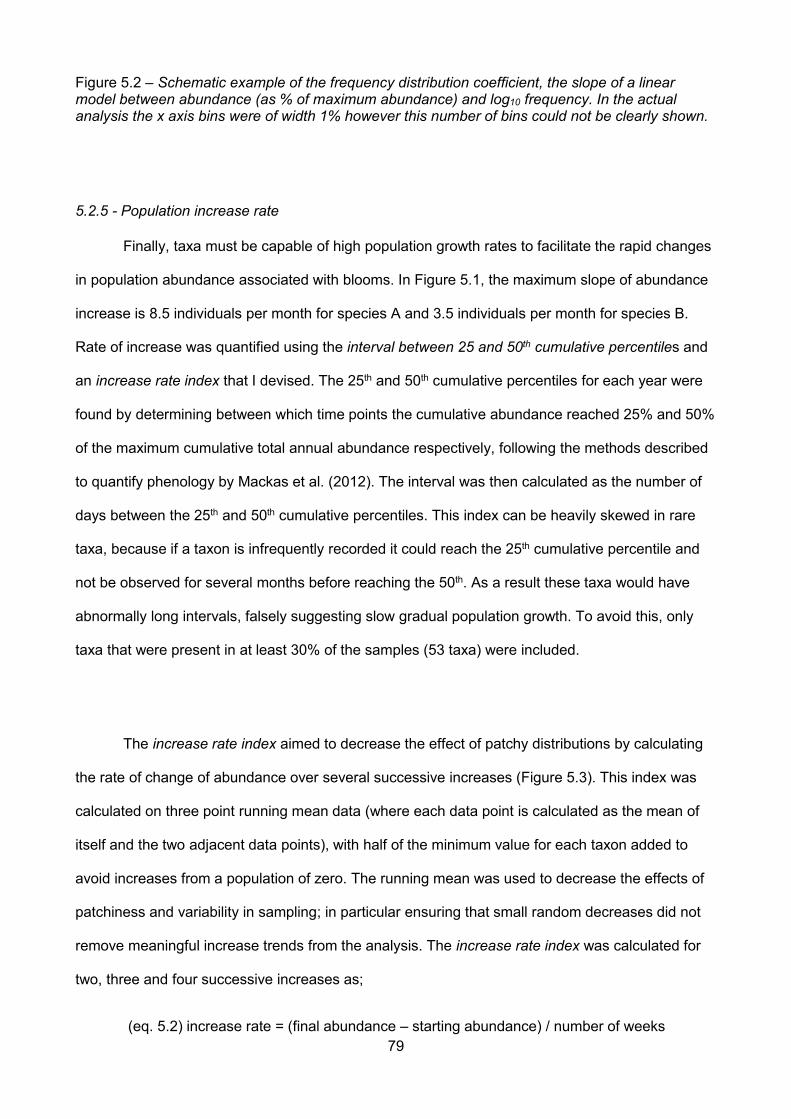
79
Figure 5.2 – Schematic example of the frequency distribution coefficient, the slope of a linearmodel between abundance (as % of maximum abundance) and log10 frequency. In the actualanalysis the x axis bins were of width 1% however this number of bins could not be clearly shown.
5.2.5 - Population increase rate
Finally, taxa must be capable of high population growth rates to facilitate the rapid changes
in population abundance associated with blooms. In Figure 5.1, the maximum slope of abundance
increase is 8.5 individuals per month for species A and 3.5 individuals per month for species B.
Rate of increase was quantified using the interval between 25 and 50th cumulative percentiles and
an increase rate index that I devised. The 25th and 50th cumulative percentiles for each year were
found by determining between which time points the cumulative abundance reached 25% and 50%
of the maximum cumulative total annual abundance respectively, following the methods described
to quantify phenology by Mackas et al. (2012). The interval was then calculated as the number of
days between the 25th and 50th cumulative percentiles. This index can be heavily skewed in rare
taxa, because if a taxon is infrequently recorded it could reach the 25th cumulative percentile and
not be observed for several months before reaching the 50th. As a result these taxa would have
abnormally long intervals, falsely suggesting slow gradual population growth. To avoid this, only
taxa that were present in at least 30% of the samples (53 taxa) were included.
The increase rate index aimed to decrease the effect of patchy distributions by calculating
the rate of change of abundance over several successive increases (Figure 5.3). This index was
calculated on three point running mean data (where each data point is calculated as the mean of
itself and the two adjacent data points), with half of the minimum value for each taxon added to
avoid increases from a population of zero. The running mean was used to decrease the effects of
patchiness and variability in sampling; in particular ensuring that small random decreases did not
remove meaningful increase trends from the analysis. The increase rate index was calculated for
two, three and four successive increases as;
(eq. 5.2) increase rate = (final abundance – starting abundance) / number of weeks
80
All increases were included in the analysis, even if multiple increases were present across
overlapping subsets of the same range of data. For each species the mean, median and maximum
increase was calculated for two, three and four successive increases. If taxa with low carbon
percentage have more bloom-like population dynamics then carbon percentage will be negatively
related to the interval between the 25th and 50th cumulative percentiles and positively related to the
increase rate index.
Figure 5.3 – Schematic example of the increase rate index, calculated for four increases as (n+4 -n) / 4. The points on the black line are data, the red line shows the range over which the increaserate for four successive increases is calculated. The green lines show two valid two step increasesacross four successive points.
5.2.6 - Testing bloom index performance
To determine the efficacy of the bloom indices, species that are known to form blooms
should be compared with those that are known for having a stable population. Pleurobrachia pileus
is a generalist zooplanktivore that spawns continuously throughout the year when food is sufficient
(Fraser, 1970). This species is capable of paedogenesis, reproduction before reaching the adult
n+4n+3
n+2
n+1
n
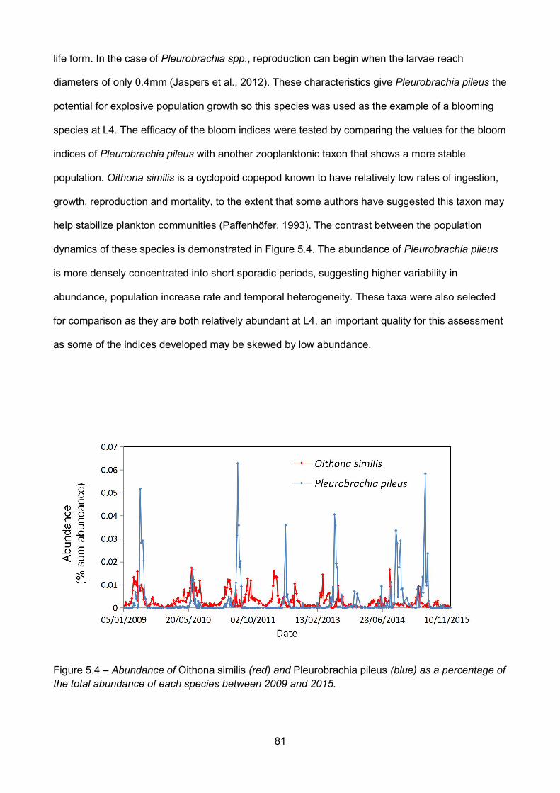
81
life form. In the case of Pleurobrachia spp., reproduction can begin when the larvae reach
diameters of only 0.4mm (Jaspers et al., 2012). These characteristics give Pleurobrachia pileus the
potential for explosive population growth so this species was used as the example of a blooming
species at L4. The efficacy of the bloom indices were tested by comparing the values for the bloom
indices of Pleurobrachia pileus with another zooplanktonic taxon that shows a more stable
population. Oithona similis is a cyclopoid copepod known to have relatively low rates of ingestion,
growth, reproduction and mortality, to the extent that some authors have suggested this taxon may
help stabilize plankton communities (Paffenhöfer, 1993). The contrast between the population
dynamics of these species is demonstrated in Figure 5.4. The abundance of Pleurobrachia pileus
is more densely concentrated into short sporadic periods, suggesting higher variability in
abundance, population increase rate and temporal heterogeneity. These taxa were also selected
for comparison as they are both relatively abundant at L4, an important quality for this assessment
as some of the indices developed may be skewed by low abundance.
Figure 5.4 – Abundance of Oithona similis (red) and Pleurobrachia pileus (blue) as a percentage ofthe total abundance of each species between 2009 and 2015.
82
The secondary aim of this chapter was to investigate whether our varios indicators of
bloom-like tendencies differed between gelatinous and non-gelatinous zooplankton. The outputs
from each of these indices were used as dependent variables in general linear models based on
the explanatory variables, carbon percentage and carbon mass. Carbon percentage of each taxon
was estimated using the table of carbon percentage presented in Appendix I, and carbon mass
following the methods also described in Chapter 2.
5.3 - Results
Species at L4 showed a range of patterns of abundance over time, with some species
occurring only as short term blooms (e.g. Evadne spp.) and others occurring consistently
throughout the year (e.g. Oithona spp.). In the case of blooming taxa, these blooms occurred at
roughly similar times each year (e.g. Pleurobrachia pileus) or were more randomly distributed (e.g.
Goniopsyllus clausi). Beroe spp. was the dominant taxa on the basis of biomass, however due to
low number of recordings (present in nine samples) and potential overestimation due to
fragmentation of the gelatinous body, it was omitted from these analyses. The taxa included vary
widely in life history, biomass and total abundance. The full list of values of each index for each
taxon is shown in Appendix III. The values for the chosen comparison species, Pleurobrachia
pileus and Oithona similis are shown in Table 5.1. The values for the full list of species were
combined with the estimates of carbon percentage, and used to create the General Linear Models
(GLMs) shown in Table 5.2.
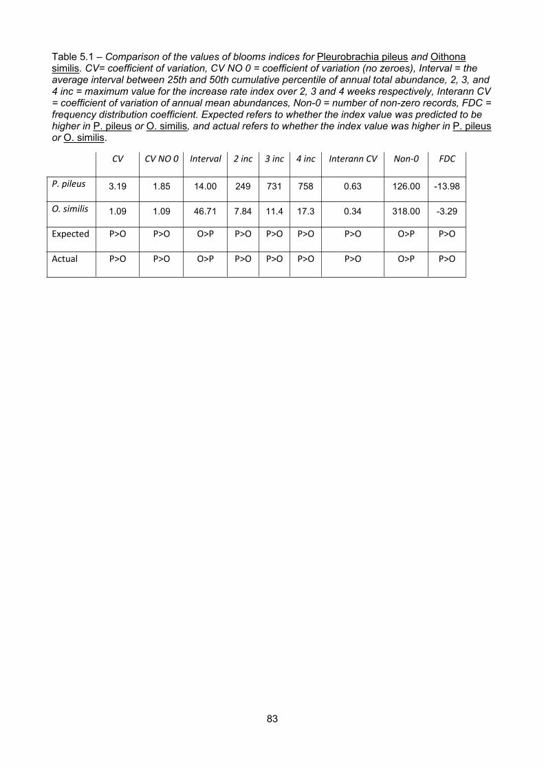
83
Table 5.1 – Comparison of the values of blooms indices for Pleurobrachia pileus and Oithonasimilis. CV= coefficient of variation, CV NO 0 = coefficient of variation (no zeroes), Interval = theaverage interval between 25th and 50th cumulative percentile of annual total abundance, 2, 3, and4 inc = maximum value for the increase rate index over 2, 3 and 4 weeks respectively, Interann CV= coefficient of variation of annual mean abundances, Non-0 = number of non-zero records, FDC =frequency distribution coefficient. Expected refers to whether the index value was predicted to behigher in P. pileus or O. similis, and actual refers to whether the index value was higher in P. pileusor O. similis.
CV CV NO 0 Interval 2 inc 3 inc 4 inc Interann CV Non-0 FDC
P. pileus 3.19 1.85 14.00 249 731 758 0.63 126.00 -13.98
O. similis 1.09 1.09 46.71 7.84 11.4 17.3 0.34 318.00 -3.29
Expected P>O P>O O>P P>O P>O P>O P>O O>P P>O
Actual P>O P>O O>P P>O P>O P>O P>O O>P P>O
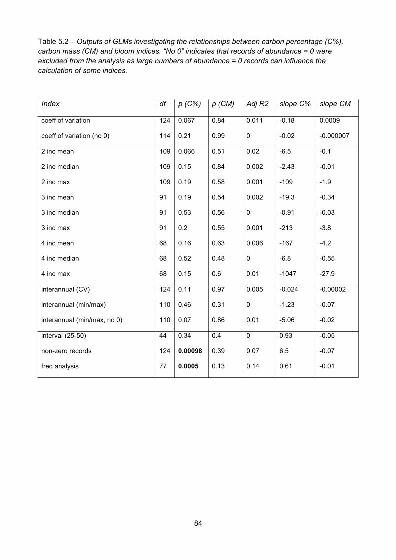
84
Table 5.2 – Outputs of GLMs investigating the relationships between carbon percentage (C%),carbon mass (CM) and bloom indices. “No 0” indicates that records of abundance = 0 wereexcluded from the analysis as large numbers of abundance = 0 records can influence thecalculation of some indices.
Index df p (C%) p (CM) Adj R2 slope C% slope CM
coeff of variation 124 0.067 0.84 0.011 -0.18 0.0009
coeff of variation (no 0) 114 0.21 0.99 0 -0.02 -0.000007
2 inc mean 109 0.066 0.51 0.02 -6.5 -0.1
2 inc median 109 0.15 0.84 0.002 -2.43 -0.01
2 inc max 109 0.19 0.58 0.001 -109 -1.9
3 inc mean 91 0.19 0.54 0.002 -19.3 -0.34
3 inc median 91 0.53 0.56 0 -0.91 -0.03
3 inc max 91 0.2 0.55 0.001 -213 -3.8
4 inc mean 68 0.16 0.63 0.006 -167 -4.2
4 inc median 68 0.52 0.48 0 -6.8 -0.55
4 inc max 68 0.15 0.6 0.01 -1047 -27.9
interannual (CV) 124 0.11 0.97 0.005 -0.024 -0.00002
interannual (min/max) 110 0.46 0.31 0 -1.23 -0.07
interannual (min/max, no 0) 110 0.07 0.86 0.01 -5.06 -0.02
interval (25-50) 44 0.34 0.4 0 0.93 -0.05
non-zero records 124 0.00098 0.39 0.07 6.5 -0.07
freq analysis 77 0.0005 0.13 0.14 0.61 -0.01

85
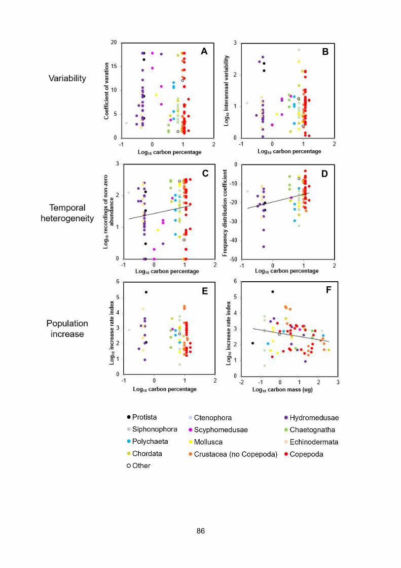
86
A B
C D
E F
87
Figure 5.5 – Relationships between carbon percentage, carbon mass and bloom indices forzooplankton taxa at the L4 sampling site. A - coefficient of variation in abundance of zooplankton atL4 as a function of log10 carbon percentage (df = 124, p = 0.013, adj R2 = 0.033, coefficient ofvariation = - 0.12 * log10 carbon percentage + 0.8), B – log10 interannual variability (maximumannual abundance / minimum annual abundance) as a function of log10 carbon percentage (df = 80,p = 0.07, adj R2 = 0.01, log10 interannual variability = - 5.06 * log10 carbon percentage + 68.3), C –log10 number of non-zero abundance records as a function of log10 carbon percentage (df = 124, p= 0.001, adj R2 = 0.07, number of non-zero records = 6.52 * carbon percentage – 58.1), D –coefficient of linear models between abundance and frequency as a function of log10 carbonpercentage (df = 77, p = 0.0005, adj R2 = 0.14, frequency distribution coefficient = 0.61 * carbonpercentage - 20.1), E – log10 maximum increase rate index across four successive increases as afunction of log10 carbon percentage (no statistically significant relationship detected), F – log10maximum increase rate index across four successive increases as a function of log10 carbon mass(df = 68, p = 0.0002, adj R2 = 0.16, log10 maximum increase rate index = - 0.46 * carbonpercentage + 1.62).
5.3.1 – Variability
5.3.1.1 – Testing of variability indices
P. pileus had higher values than O. similis for all three indices of population variability;
coefficient of variation, ratio between the maximum and minimum mean annual abundances and
coefficient of variation of mean annual abundances. This suggests that these indices could be
effective for quantifying the variability associated with blooming in zooplankton.
5.3.1.2 – Effect of carbon percentage on variability indices
There was limited support for a relationship between carbon percentage and variability in
abundance, but no relationship with carbon mass. No effect of either carbon mass or carbon
percentage was observed on coefficient of variation at p<0.05. The full analysis including all data
(Figure 5.5A, p = 0.067) and the analysis omitting zeroes and meroplanktonic taxa (p = 0.07) were
approaching 5% significance levels. In both analyses, the slope with increasing carbon percentage
was negative, offering limited support that more gelatinous taxa tend to be more variable at L4.
There was a marginally significant (0.07) negative effect of carbon percentage on interannual
variability (max / min annual abundance), potentially suggesting that gelatinous taxa may be more
88
variable than less gelatinous taxa (Figure 5.5B). However, the R2 values for the relationships
between variability and carbon mass and carbon percentage were very low, suggesting that other
factors were more important in determining variability at L4.
5.3.2 - Temporal heterogeneity
5.3.2.1 – Testing of temporal heterogeneity indices
O. similis had higher values than P. pileus for the indices of temporal heterogeneity;
number of non-zero records and frequency distribution coefficient. This follows the predictions
made in the methods, suggesting that the indices used were capable of detecting the differences in
temporal heterogeneity between the two species, and may be more widely applicable.
5.3.2.2 – Effect of carbon percentage on temporal heterogeneity indices
There was strong support for a relationship between temporal heterogeneity in abundance
and carbon percentage, but no relationship with carbon mass. There was a highly significant
positive relationship between carbon percentage and number of non-zero records, more gelatinous
taxa were less frequently recorded at L4 (Figure 5.5C). Similarly, a highly significant positive
relationship was observed between carbon percentage and the frequency distribution coefficient
(Figure 5.5D), which suggests that the abundance of gelatinous taxa was more heterogeneously
distributed through time than other taxa.
5.3.3 - Population increase rate
5.3.3.1 – Testing of population increase rate indices
As predicted, the increase rate index of Pleurobrachia pileus was higher and the interval
between the 25th and 50th cumulative percentiles was shorter than that of O. similis. These indices
89
were capable of detecting the differences in the relative increase rates of these species, and may
be effective more widely.
5.3.3.2 – Effect of carbon percentage on population increase rate indices
There was no significant relationship between increase rate indices and carbon percentage,
but there was a significant negative relationship between carbon mass and increase rate (Figure
5.5E, F). The mean, median and maximum increase rates were calculated for two, three and four
successive increases. To ensure that the transformation used on the data was not influencing the
result a sensitivity analysis was performed. The original transformation, adding half the minimum
abundance for each species, was substituted to adding 1 to abundance. No versions of the
analysis could detect any significant relationship between increase rate and carbon percentage. In
addition, the 25th – 50th cumulative interval was not affected either by carbon percentage or carbon
mass.
5.4 – Discussion
5.4.1 – Variability in abundance
5.4.1.1 – Are the variability-based bloom indices effective?
The indices tested for variability in abundance were coefficient of variation, ratio between
the maximum and minimum mean annual abundances and coefficient of variation of mean annual
abundances. For these indices, P. pileus had higher values than O. similis as predicted. All of
these indices were based on ratios and therefore scale to allow the comparison of taxa with
different mean abundances. This is useful as many taxa are rare and therefore their mean
abundance is lower than that of other more common species. It is worth noting that the coefficient
of variation was calculated excluding zeros, the value for P. pileus decreased but the value for O.
similis was relatively unchanged. This was the result of the high number of zero abundance
90
records in P. pileus relative to O. similis increasing variance. This difference was used in both the
indices of temporal heterogeneity as another way to categorise bloom-like population dynamics.
The indices based on interannual variability need several years of data to be useful, however the
coefficient of variation could be used with potentially any period of repeated records. Its strength as
an index will increase with additional records and should preferentially include at least one year to
cover the full seasonal cycle.
5.4.1.2 – The relationship between carbon percentage and variability in abundance
There was limited evidence, both from the coefficient of variation and interannual variability,
that more gelatinous taxa might be more variable in abundance at L4. One potential reason for this
could be the influence of life history. Many gelatinous taxa have benthic stages such as polyps or
hydroids (25 of 32 of taxa with carbon percentage <1%). The influence of a metagenic lifecycle
with benthic polyps was highlighted in the bloom definition. Biomass is accumulated in the benthic
stages of these organisms, and the release of planktonic larvae can increase populations faster
than would be expected based on the existing planktonic population (Purcell et al., 2007). This
benthic dependency is also observed in many of the less gelatinous taxa. However, the influence
of benthic stages seem unlikely to be the primary cause of greater variation in abundance, as the
average coefficient of variation of gelatinous taxa with benthic stages and without benthic stages
was very similar (1.75 and 1.80 respectively). If the relationship between coefficient of variation
and carbon percentage was driven by recruitment from the benthic stages of gelatinous
zooplankton then a negative relationship between increase rate and carbon percentage would be
expected; this is not observed.
91
5.4.2 - Temporal heterogeneity
5.4.2.1 – Are the temporal heterogeneity based bloom indices effective?
The indices used to investigate temporal heterogeneity were the number of non-zero
records and the frequency distribution coefficient. For both indices, O. similis had higher values
than P. pileus, as predicted. These indices are useful tools for comparing different species as they
do not require the same amount of data as the others. It is possible to compare taxa with less than
one year of data, and generate a more meaningful index than some of the others presented.
However, these indices are potentially less effective than the others for use with rare species. For
instance, the number of non-zero records in a taxon could be low as a result of only encountering
that taxa during a short bloom. Alternatively, a low number of non-zero records could indicate that
as a result of rarity, the species was recorded relatively few times over the course of the sampling
period. This drawback, while lessened by normalisation, is also present in the frequency
distribution coefficient. For this reason, I recommend that these indices are only used with
relatively abundant taxa.
5.4.2.2 – Discussing the relationship between carbon percentage and temporal heterogeneity
There was a strong positive relationship between carbon percentage and number of non-
zero records; taxa with higher carbon percentage were recorded more frequently. However, this
index tends to be heavily skewed in species that form aggregations, as the probability of recording
a specific taxon is affected by their distribution. To remedy this the frequency distribution analysis
was also performed, with similar results. The frequency distribution of more gelatinous taxa tended
to be steeper, implying the abundance of these species was concentrated into shorter periods,
seen as spikes in the abundance profiles. This finding follows the predicted pattern, as gelatinous
species are normally considered to be ephemeral (at least in their medusa phase) and exploit
temporally and spatially patchy good conditions (Lucas and Dawson, 2014). For instance, many
cnidarians and ctenophores have a generalist diet, allowing them to survive in a range of
environments where food is both patchy and not diverse (Richardson et al., 2009). This contrasts
92
with several copepod taxa such as Calanus helgolandicus and Oithona spp., which are noted for
their relatively consistent abundance (and therefore shallow frequency distribution) throughout the
year (Maud et al., 2015; Atkinson et al., 2015).
5.4.3 - Population increase rate
5.4.3.1 – Are the population increase based bloom indices effective?
Generating estimates of population increase rate using time series data is difficult because
increases in recorded abundance are not necessarily representative of increases in abundance, it
could be due to patchiness or active aggregation. The two indices used for population increase
were the interval between the 25th and 50th cumulative percentiles and the increase rate index. The
interval was shorter for P. pileus than O. similis as predicted. This was due to the abundance of P.
pileus being concentrated into a shorter period than O. similis. The index was effective in these two
taxa however it is highly sensitive to the annual total abundance, and for that reason this index
should not be used with very rare taxa.
The increase rate index was devised as a way to estimate increase rate without being as
sensitive to patchiness. The increase rate of P. pileus was expected to be higher than that of O.
similis, with the difference increasing with the number of successive increases investigated. This
was observed in the data, suggesting that this index may be an effective way of comparing relative
abundance increase. There are however still potential issues with this method, such as consistent
advection into sample area. This index is also highly sensitive to starting abundance, as it is based
on the ratio between starting and finishing abundances, not the number of individuals increased
per time point. Finally, this approach is somewhat reliant on a good time series, as the more
reliable three and four successive increase indices need consistent present records, and several
sets of successive increase are required to form reasonable comparisons.

93
5.4.3.2 – Discussing the relationship between carbon percentage and increase rate
One of the identified prerequisites for bloom formation was rapid increase in population
(section 5.2.5). Therefore, if bloom-like dynamics are observed in gelatinous zooplankton but no
other taxa then we might expect there to a negative relationship between carbon percentage and
increase rate. While carbon mass was observed to have a strong negative effect on increase rate
(Fig 5.9) consistent with higher growth rates and shorter generation times of smaller animals
(Pianka, 1970), there was no relationship found between increase rate and carbon percentage.
The highest population increase rates were observed in taxa with high reproductive outputs that
did not reproduce sexually as planktonic adults e.g. the planktonic protist, Noctiluca scintillans. The
cladocerans, Evadne spp. and Podon spp., were also within the top 5% of maximum population
increase rates. These taxa are also capable of asexual reproduction through parthenogenesis
(Mullin and Onbe, 1992; Kim and Onbe, 1989), and therefore are expected to have massive
population increase potential relative to other metazoans. The other taxa that had high increase
rates were meroplanktonic taxa, especially rhizocephalan nauplii. This is a result of these larvae
being generated and released from adults on the seabed, and therefore not relying solely on the
planktonic population to increase abundance. The only taxon that was holoplanktonic and was
within the top 10 increase rates observed was Appendicularia, most likely Oikopleura dioica,
known to have short generations times (Hopcroft and Roff, 1995) and extremely efficient feeding
(King and Azam, 1980). Overall, increase rate appeared to be more a function of reproductive
strategy, for example pulsed reproduction from the seabed controlling planktonic population
increases, rather than carbon percentage.
5.4.4 – Are taxa with higher carbon percentages also blooming?
Taxa that are more gelatinous may be more variable in abundance and have shorter
periods of significant presence in the zooplankton, but there was no evidence that these had a
faster rate of population increase. Based on these observations, are taxa with lower carbon
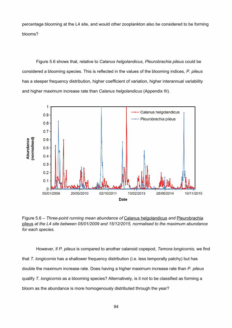
94
percentage blooming at the L4 site, and would other zooplankton also be considered to be forming
blooms?
Figure 5.6 shows that, relative to Calanus helgolandicus, Pleurobrachia pileus could be
considered a blooming species. This is reflected in the values of the blooming indices, P. pileus
has a steeper frequency distribution, higher coefficient of variation, higher interannual variability
and higher maximum increase rate than Calanus helgolandicus (Appendix III).
Figure 5.6 – Three-point running mean abundance of Calanus helgolandicus and Pleurobrachiapileus at the L4 site between 05/01/2009 and 15/12/2015, normalised to the maximum abundancefor each species.
However, if P. pileus is compared to another calanoid copepod, Temora longicornis, we find
that T. longicornis has a shallower frequency distribution (i.e. less temporally patchy) but has
double the maximum increase rate. Does having a higher maximum increase rate than P. pileus
qualify T. longicornis as a blooming species? Alternatively, is it not to be classified as forming a
bloom as the abundance is more homogenously distributed through the year?
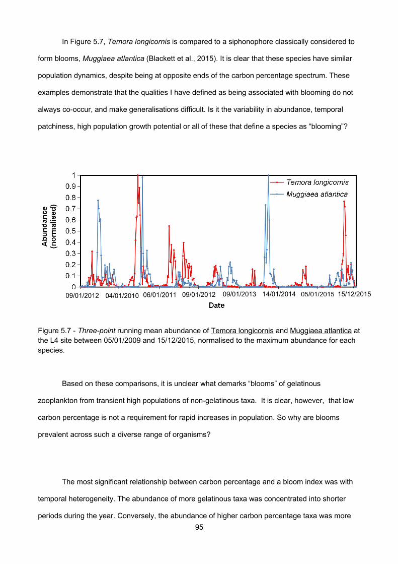
95
In Figure 5.7, Temora longicornis is compared to a siphonophore classically considered to
form blooms, Muggiaea atlantica (Blackett et al., 2015). It is clear that these species have similar
population dynamics, despite being at opposite ends of the carbon percentage spectrum. These
examples demonstrate that the qualities I have defined as being associated with blooming do not
always co-occur, and make generalisations difficult. Is it the variability in abundance, temporal
patchiness, high population growth potential or all of these that define a species as “blooming”?
Figure 5.7 - Three-point running mean abundance of Temora longicornis and Muggiaea atlantica atthe L4 site between 05/01/2009 and 15/12/2015, normalised to the maximum abundance for eachspecies.
Based on these comparisons, it is unclear what demarks “blooms” of gelatinous
zooplankton from transient high populations of non-gelatinous taxa. It is clear, however, that low
carbon percentage is not a requirement for rapid increases in population. So why are blooms
prevalent across such a diverse range of organisms?
The most significant relationship between carbon percentage and a bloom index was with
temporal heterogeneity. The abundance of more gelatinous taxa was concentrated into shorter
periods during the year. Conversely, the abundance of higher carbon percentage taxa was more
06/01/201104/01/2010 09/01/2012 15/12/201509/01/2013 14/01/2014 05/01/201509/01/2012
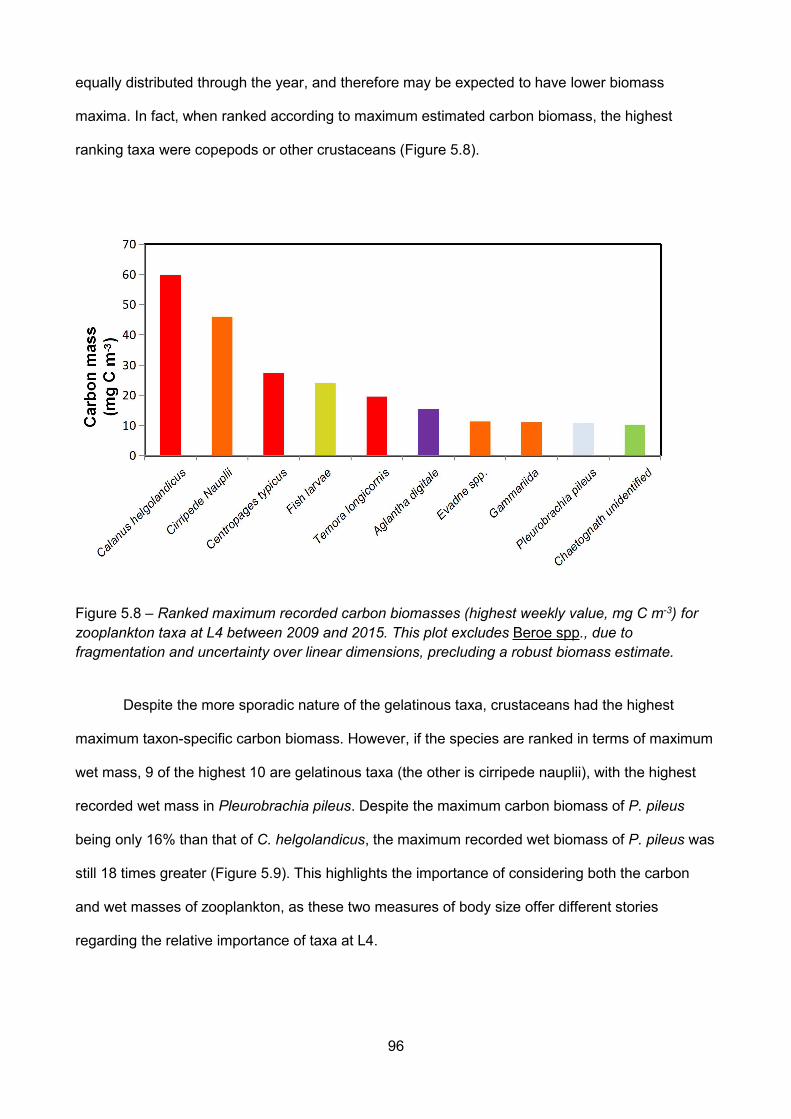
96
equally distributed through the year, and therefore may be expected to have lower biomass
maxima. In fact, when ranked according to maximum estimated carbon biomass, the highest
ranking taxa were copepods or other crustaceans (Figure 5.8).
Figure 5.8 – Ranked maximum recorded carbon biomasses (highest weekly value, mg C m-3) forzooplankton taxa at L4 between 2009 and 2015. This plot excludes Beroe spp., due tofragmentation and uncertainty over linear dimensions, precluding a robust biomass estimate.
Despite the more sporadic nature of the gelatinous taxa, crustaceans had the highest
maximum taxon-specific carbon biomass. However, if the species are ranked in terms of maximum
wet mass, 9 of the highest 10 are gelatinous taxa (the other is cirripede nauplii), with the highest
recorded wet mass in Pleurobrachia pileus. Despite the maximum carbon biomass of P. pileus
being only 16% than that of C. helgolandicus, the maximum recorded wet biomass of P. pileus was
still 18 times greater (Figure 5.9). This highlights the importance of considering both the carbon
and wet masses of zooplankton, as these two measures of body size offer different stories
regarding the relative importance of taxa at L4.
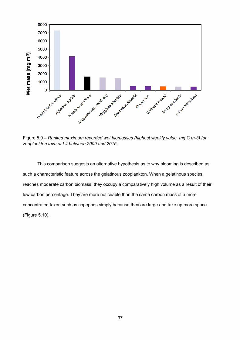
97
Figure 5.9 – Ranked maximum recorded wet biomasses (highest weekly value, mg C m-3) forzooplankton taxa at L4 between 2009 and 2015.
This comparison suggests an alternative hypothesis as to why blooming is described as
such a characteristic feature across the gelatinous zooplankton. When a gelatinous species
reaches moderate carbon biomass, they occupy a comparatively high volume as a result of their
low carbon percentage. They are more noticeable than the same carbon mass of a more
concentrated taxon such as copepods simply because they are large and take up more space
(Figure 5.10).
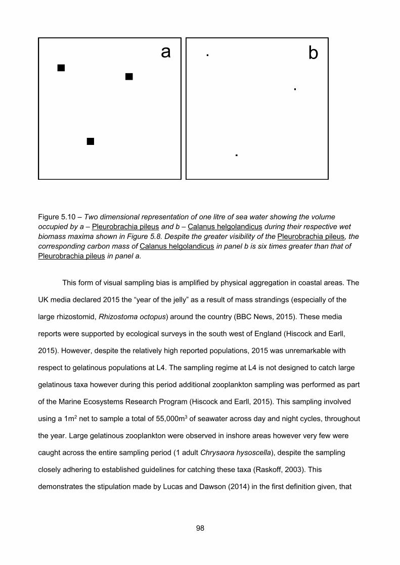
98
Figure 5.10 – Two dimensional representation of one litre of sea water showing the volumeoccupied by a – Pleurobrachia pileus and b – Calanus helgolandicus during their respective wetbiomass maxima shown in Figure 5.8. Despite the greater visibility of the Pleurobrachia pileus, thecorresponding carbon mass of Calanus helgolandicus in panel b is six times greater than that ofPleurobrachia pileus in panel a.
This form of visual sampling bias is amplified by physical aggregation in coastal areas. The
UK media declared 2015 the “year of the jelly” as a result of mass strandings (especially of the
large rhizostomid, Rhizostoma octopus) around the country (BBC News, 2015). These media
reports were supported by ecological surveys in the south west of England (Hiscock and Earll,
2015). However, despite the relatively high reported populations, 2015 was unremarkable with
respect to gelatinous populations at L4. The sampling regime at L4 is not designed to catch large
gelatinous taxa however during this period additional zooplankton sampling was performed as part
of the Marine Ecosystems Research Program (Hiscock and Earll, 2015). This sampling involved
using a 1m2 net to sample a total of 55,000m3 of seawater across day and night cycles, throughout
the year. Large gelatinous zooplankton were observed in inshore areas however very few were
caught across the entire sampling period (1 adult Chrysaora hysoscella), despite the sampling
closely adhering to established guidelines for catching these taxa (Raskoff, 2003). This
demonstrates the stipulation made by Lucas and Dawson (2014) in the first definition given, that
ba
99
not all high populations represent true blooms. It is also worth noting that most gelatinous taxa are
not large, and that many small gelatinous do not form blooms following their definition.
This discussion is not intended to trivialise blooms, as the ecological and biogeochemical
implications of bloom events are clearly significant. This discussion intends instead to address the
extent to which low carbon percentage drives our interpretation of jellyfish blooms. When we
encounter a jellyfish bloom it is often interpreted as an extraordinary concentration of biomass of a
particular organism, but interpreting a bloom as a normal concentration of an extraordinary animal
may be more appropriate.

100

101
CHAPTER 6 – Body size as a function of carbon mass and
carbon percentage
102
6.1 - Introduction
Despite body size influencing all aspects of an organism’s biology, it is an ambiguous term.
Body size refers not to a single quality but to a range of variables that are related to different
aspects of the physiology and ecology an organism. As a result of this, for information on the body
size of an organism to be informative, it must be an appropriate measure for the question being
investigated. For instance, when relating metabolic rate to body size, carbon or nitrogen mass is
often most appropriate and the latter has been used widely (Brown et al., 2005, Kiorboe and Hirst,
2014). For investigating trends in metabolism, if we instead choose length as our measure of body
size, we would find that organisms with highly elongated bodies might skew the relationship. We
might expect the 40m long (but 3cm wide) siphonophore, Praya dubia to have a higher metabolic
rate than that of a 25m long blue whale, despite the whale being many times greater in mass.
Conversely, when considering whether a prey item is capable of being eaten by a gape-limited
predator, length along the longest dimension will be of paramount importance, especially for taxa
with long spines such as Porcellana platycheles larvae.
If all organisms were the same shape and composition then different measures would not
be so necessary, however massive variation exists both inter and intraspecifically. While the
variability between carbon mass and length as a result of shape change is readily accepted and
even applied (Hirst et al., 2014), the variability between carbon mass and wet mass observed in
zooplankton has not been considered in detail. This variability was summarised in the negative
relationship between carbon mass and carbon percentage presented in chapter 3, and is explored
in greater detail below.
As carbon mass and carbon percentage have different effects on organismal biology,
investigating how taxa are distributed in this trait space might help to shed light on how the body
size of plankton influences their biology and evolution. The aim of this chapter is to investigate the
103
form and implications of the relationship between carbon mass and carbon percentage through the
following objectives;
- Determine the relationship between carbon mass and carbon percentage using the meta-
analysis and L4 datasets.
- Investigate the spread around this relationship, focussing on the areas of trait space that
are not populated with taxa.
- Discuss other taxa that are not gelatinous but show analogous decoupling between
metabolic and ecological body size (i.e. pseudo-gelatinous taxa)
- Investigate how biomass is distributed in this trait space in a real assemblage using the L4
dataset
6.2 - What is the relationship between carbon percentage and carbon mass, and why is itimportant?
In Chapter 3, I found a negative relationship between carbon mass and carbon percentage
(Figure 3.4). The only other study that has investigated this relationship is by Molina-Ramirez et al.
(2015) exploring the relationship between carbon mass and wet mass of a range highly gelatinous
taxa (cnidarians, ctenophores, salps and doliolids). These authors separated the taxa on the basis
of feeding mode; carbon percentage decreased with increasing carbon mass in filter feeders (salps
and doliolids), while in carnivores (cnidarians and ctenophores) carbon percentage was constant.
The results in Chapter 3 followed the pattern of decreasing carbon percentage observed for the
salps and doliolids in the study by Molina-Ramirez et al. (2015). However, in my study, carbon
percentage decreased with increasing carbon mass across all taxa, regardless of feeding mode.
This difference could be the result of including the full range of zooplankton in Chapter 3, in
contrast to just highly gelatinous taxa in the study by Molina- Ramirez et al. (2015).
In the study by Molina-Ramirez et al. (2015), the linear relationships between carbon mass
and wet mass were used to derive single values of carbon percentage for ctenophores (0.23% ±
104
0.14%) and cnidarians (1.77% ± 2.44%). In the meta-analysis presented in Chapter 3, carbon
percentage within the cnidarians alone ranged from 0.02 and 2.22%, corresponding to a 110-fold
difference in wet mass at equivalent carbon mass. While attributing a single value to a wide range
of species can provide some simplification, it could lead to large errors. For instance, the range of
carbon percentage seen in the cnidarians alone in Chapter 2 could correspond to a doubling in
growth rate at the same carbon mass.
In the study by Molina-Ramirez et al. (2015), whether carbon percentage decreased with
increasing carbon mass across species was dependent on feeding mode. Carnivores (defined as
cnidarians and ctenophores) were found to have a fixed carbon percentage of 1.77% ± 2.44% at all
carbon masses. Chapter 4 investigated the carbon percentage of Aurelia aurita throughout early
development. On the basis of the findings of Molina-Ramirez et al. (2015) the carbon percentage of
Aurelia aurita should not vary with carbon mass as it is a carnivore. However in chapter 3, it was
observed that Aurelia aurita ephyrae diluted carbon centrations from 2.3% to 0.1% through
ontogeny. This could be a result of Chapter 4 investigating intraspecific variability and the previous
study by Molina Ramirez et al. (2015), interspecific variability. However, if the feeding mode
hypothesis advanced by Molina-Ramirez et al. (2015) is correct then it should not matter whether
the variation in carbon mass is interspecific or intraspecific. An alternative cause could be that the
studies are investigating different scales, Chapter 4 investigated between 0.01 and 0.2 mg C in
contrast to the range of between 0.01 and 100000 mg C in Molina Ramirez et al. (2015). Leaving
aside contrasts with previous studies, Chapter 4 is the first investigation of how the carbon and wet
masses interact to determine feeding and growth during development.
6.3 - Carbon percentage – carbon mass trait space
Figure 6.1 shows the relationship between carbon mass and carbon percentage and
demonstrates the distribution of species in this trait space. Inspection of this figure shows that
there are areas of trait space which appear to be without species. Throughout the thesis I have
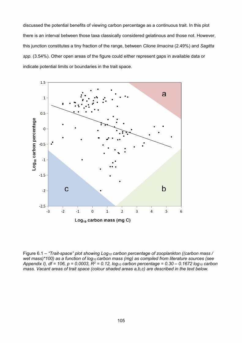
105
discussed the potential benefits of viewing carbon percentage as a continuous trait. In this plot
there is an interval between those taxa classically considered gelatinous and those not. However,
this junction constitutes a tiny fraction of the range, between Clione limacina (2.49%) and Sagitta
spp. (3.54%). Other open areas of the figure could either represent gaps in available data or
indicate potential limits or boundaries in the trait space.
Figure 6.1 – “Trait-space” plot showing Log10 carbon percentage of zooplankton ((carbon mass /wet mass)*100) as a function of log10 carbon mass (mg) as compiled from literature sources (seeAppendix I), df = 106, p = 0.0003, R2 = 0.12, log10 carbon percentage = 0.30 – 0.1672 log10 carbonmass. Vacant areas of trait space (colour shaded areas a,b,c) are described in the text below.
a
bc
106
6.3.1 - Area a: high carbon mass and high carbon percentage
The first area of empty trait space highlighted in Figure 6.1 (region a marked in red)
indicates an absence of data for taxa with more than 5% carbon that exceed ~250 mg carbon. This
maximum carbon mass is seen in adult Euphausia superba (approximately 65 mm maximum
length: Atkinson et al., 2006), that are one of the largest epipelagic crustaceans. There are clearly
pelagic, carbon-rich taxa with higher carbon masses, from fish to whales, but this body mass very
roughly marks the transition from crustaceans to these nektonic life forms. This could be a result of
the scope for growth scaling discussed above but there are alternative hypotheses, in particular
buoyancy and oxygen requirement (Alexander, 1990; Verberk and Atkinson, 2013).
Large, high carbon percentage animals require supplementary methods to regulate
buoyancy, such as constant swimming in krill (Kils, 1981). These methods, whether based on
motion or regulation of a swim bladder carry an associated cost that could further favour the scope
for growth of more gelatinous taxa at high carbon masses. In the case of highly gelatinous taxa, a
much greater percentage of the body is sea water, and therefore the energetic cost of buoyancy
regulation (sometimes through the exclusion of sulphate ions, Bidigare and Biggs, 1980) at a given
body size is likely to be much lower than that of a high carbon percentage organism.
Oxygen transfer is another factor that could restrict the evolution of large, high carbon
percentage zooplankton. Respiration rate is a function of carbon mass, so the respiratory
requirement of high carbon mass animals is high (despite carbon specific respiration rate typically
decreasing with increasing carbon mass (Kleiber, 1932; Brown et al. 2004; Glazier, 2006)). To be
larger, organisms have had to develop means to increases the rate of oxygen transfer to meet the
increased total respiratory requirement associated with large body size. All of these methods,
including convolution of the body surface or a full respiratory systems increase the rate of oxygen
transfer to exceed the rate that would be possible through passive diffusion across the body
surface alone. The methods used to facilitate oxygen transfer depend on the taxon, however using
107
a simple geometric model it is possible to model the effect of variation in carbon percentage on
tissue oxygen availability in a similar manner to feeding rate. Oxygen transfer is a function of
surface area which is dependent on wet mass. Therefore, an organism with a lower carbon
percentage will have a higher surface area to carbon mass ratio than a geometrically similar
organism with higher carbon percentage. This suggests that decreasing carbon percentage
increases carbon specific oxygen availability, potentially alleviating an oxygen limitation boundary.
This is a considerable oversimplification, as organisms rarely grow isometrically (with considerable
implication to metabolic scaling (Glazier et al., 2015)) and not all organisms are identical in shape.
Furthermore, the most gelatinous taxa (cnidarians and ctenophores) maintain low core body
oxygen percentage, such that diffusion gradients into the surface tissues are greater, and oxygen
transfers through the tissues at a greater rate (Thuesen et al., 2005).
Irrespective of how carbon percentage affects respiratory requirements, the resilience of
low carbon percentage taxa to hypoxia is well documented (Purcell et al., 2001; Decker et al., 2004;
Thuesen et al., 2005; Elliot et al., 2012). Even allowing for morphological differences, it is clear that
reduced carbon percentage has the potential to reduce the effects of oxygen limitation in both the
context of hypoxic environments and determining maximum body size.
6.3.2 - Area b: high carbon mass and low carbon percentage
The organisms with the highest carbon masses are between 1.2% and 0.28% carbon, not
at the minimum carbon percentage of approximately 0.05%, thus leaving area b blank (Figure 6.1,
region b marked in green). It is possible that taxa that have lower carbon percentage cannot have
carbon masses this high due to their physical fragility. While I cannot present conclusive data, taxa
with lower carbon percentage tend to have particularly diaphanous bodies even for gelatinous taxa.
Among the least gelatinous scyphomedusae are the rhizostomids with carbon percentage of up to
1.21%. These taxa are well known for their comparative rigidity, supporting their shape outside of
108
water, sporting common names such as the cannonball jellyfish and forming the basis of jellyfish
fisheries (Brotz et al., 2016). In contrast, the lowest carbon percentages are observed in the lobate
ctenophores, in particular the mesopelagic Bathycyroe fosteri. The bodies of these taxa are very
fragile and readily fragment under minor physical stress (pers. obs.). However, large lobate
ctenophores do exist, such as Leucothea pulchra (Matsumoto, 1988), capable of reaching lengths
of 25 cm. This could suggest that the gap in the trait space may be in part due to inadequate
sampling techniques for large, highly gelatinous taxa. The use of methods that involve minimal
changes in water pressure or physical disturbance, such as those used with remotely operated
vehicles might help to populate this area of trait space.
6.3.3 - Area c: low carbon mass and low carbon percentage
Finally, the lower left quadrant (Figure 6.1, region c in blue) is sparsely populated,
indicating that there are relatively few taxa with both very low carbon percentage and carbon
masses. This could indicate a lower limit, such that for a given carbon mass there is a minimum
possible carbon percentage. In Chapter 3 we saw that ephyrae dilute from 2.3% carbon to 0.1% as
they increase from 0.01 mg C to 0.17 mg, fitting within this potential boundary. This absence of
taxa could also represent a potential sampling bias caused by the use of nets, or inappropriate
mesh sizes (Raskoff et al., 2003). Several studies using a range of in-situ, visual sampling
techniques have demonstrated the serial underestimation of small gelatinous taxa caused by net
sampling (Luo et al., 2014; Cross et al., 2015)
6.4 - Pseudo gelatinous taxa
Data for pseudo gelatinous taxa seem to counter the trends documented in this thesis.
Pseudo gelatinous taxa are defined here as any organism that artificially increases its effective
body volume without directly increasing the wet mass of the body. There is a range of such
organisms in the plankton, in particular appendicularians and thecosome pteropods. Both groups
(from different phyla) use external mucosal structures for feeding, increasing their feeding potential.
109
A terrestrial analogue is the use of web by a spider to catch food. In all instances the animals
increase their effective influence on the environment without increasing their carbon mass and
therefore respiratory requirements. However, the creation and processing of these external
structures is likely costly, contrasting with the seemingly low cost of reducing carbon percentage.
A conceptual difficulty here lies in what is defined as the carbon and wet masses of the
organism. An appendicularian is wholly dependent on the mucosal house for feeding so completely
excluding the house from measurements of mass is not representative of the organism as whole.
However, the house is not attached to the animal and is not living. Likewise, it seems incorrect to
calculate carbon specific feeding rate including the carbon that makes up the house, as it is not
metabolically active. This is analogous to issues over whether to include storage lipid in estimates
of carbon specific metabolic rate (Vidal and Whitledge, 1982). However if wet mass specific
feeding rate is calculated on the basis of the animal alone, the result will be anomalous and not
reflect the trophic strategy or morphology of the animal. This difficulty was also highlighted in a
further contrast between this thesis and the study of Molina Ramirez et al. (2015). In their study,
cnidarians included the cystonect siphonophore Physalia physalis and the chondrophore Velella
velella. While these taxa belong to different groups in the Phylum Cnidaria, they are functionally
united by the presence of a rigid float (similar to cartilage) that maintains their position in the
neuston. This float is largely metabolic inactive (Larimer and Ashby, 1962) and is not involved in
prey capture, therefore including the metabolically inactive float in calculations of carbon mass of
the animal is analogous to examples described above. If we include the float in our estimate of
carbon mass and make the implicit assumption that carbon mass is indicative of the amount of
metabolically active tissue, then we could run into errors. This also explains why Physalia physalis
had a carbon percentage that was significantly greater than that of any other cnidarian (9.02%,
Molina-Ramirez et al., 2015). There are examples where including and excluding both internal and
external structures can be unrepresentative of carbon or wet mass, so a more subtle form of
definition may be needed. One example could be the separation between structure and reserve
advanced by the dynamic energy budget model (Kooijman, 2010; Sousa et al., 2010). While for
110
many organisms, whole body measurements of carbon and wet mass will be most appropriate, the
exceptions will often demonstrate interesting evolutionary strategies such as those detailed above.
6.5 - Carbon mass and carbon percentage at the L4 study site
The figure and discussion above indicate the potential trait space of carbon mass and
carbon percentage. Therefore, it could be instructive to compare how this potential trait space
corresponds to a real assemblage. For this, individual carbon mass, carbon percentage and taxon
biomass were calculated for each taxon at the L4 sampling site (Figure 6.2).
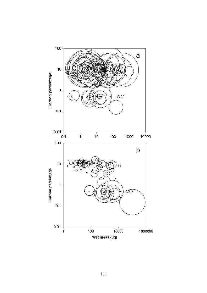
111
112
Figure 6.2 – Distribution of mean zooplankton biomass across axes of log10 carbon percentage and
log10 individual carbon mass (a) or log10 individual wet mass (b) at the L4 sampling site between
1988 and 2016. Mean biomass (mg C m-3 for panel a and mg WM m-3 for panel b) for each species
was obtained by averaging across all sampling time points. Larger bubbles indicate higher mean
taxon biomass. Carbon masses were measured and carbon percentages were assigned as
described in Chapter 5.
Firstly, the trait distribution at L4 follows that defined in Figure 3.4 with carbon mass
increasing with decreasing carbon percentage. The majority of the carbon mass at L4 is found
between 6.4 and 12.6% carbon, including the majority of the calanoid copepods. Within this carbon
percentage range, between 1 and 10 µg C is particularly biomass laden, including Acartia clausi,
Centropages spp and Para/Clauso/Cteno/Pseudocalanus.
The distribution of mean wet mass across a trait space of wet mass and carbon percentage
is shown in Figure 6.2b. Beroe spp. were omitted due to potential identification and recording
issues. This distribution differs from that of Figure 6.2a, with mean wet mass more evenly
distributed across the range. There is less biomass in the intermediate gelatinous range (0.8% < x
< 6.4%) despite this range including ecologically important taxa such as chaetognaths. Greater
mean wet mass is observed towards to the more gelatinous end of the spectrum, as moderate
carbon masses in this area correspond to disproportionately high wet masses. The greatest mean
carbon mass was found in an intermediate carbon mass bracket (<10 mg C), but the greatest
mean wet mass was found in the maximum wet mass bracket (>100000 mg WM). This suggests
that when gelatinous taxa dominate in wet mass terms it is because of relatively fewer larger
individuals, rather than many small individuals. When the community is assessed in carbon mass
terms (6.2a) the crustacean taxa are dominant but in wet mass terms (6.2b) the more gelatinous
taxa are more significant, following the pattern seen in Chapter 5. The direct effect of carbon
113
percentage on feeding and growth rates and the radical difference between zooplankton
assemblages viewed from carbon and wet mass terms highlights the importance of carbon
percentage to understanding plankton biology.
6.6 - Conclusion
This chapter has demonstrated that the relationship between carbon mass and carbon
percentage can suggest how different constraints shape zooplanktonic taxa. A whole range of
different parameters can influence the size of organisms, including buoyancy and oxygen
availability. The adoption of a more gelatinous body may increase the maximum carbon mass
possible for an organism to live a planktonic lifestyle. More gelatinous taxa are closer to seawater
in density and therefore potentially expend less energy on buoyancy regulation than denser
organisms. Similarly, organisms with a more gelatinous body will have lower respiratory demands
at the same wet mass, potentially allowing them to survive areas of lower oxygen concentration.
While these examples are tied specifically to the environment experienced by zooplankton, the
variability seen here has wider analogous significance. More generally, variation in the relationship
between carbon and wet mass represents a decoupling between metabolic and physiological body
size. This decoupling occurs in a wide variety of organisms from all environments, including
spiders. When the decoupling between metabolic and physiological body size is appreciated,
ecosystems can be viewed through either lens, highlighting the importance of using the appropriate
index of body size for the question being investigated.

114

115

116
CHAPTER 7 – Concluding discussion
117
7.1 - Introduction
This thesis has examined the merit of using carbon percentage as a trait for understanding
different aspects of zooplankton biology, over a range of scales and using different approaches
involving experiments, time series analysis and meta-analysis. This chapter begins by
summarising the results of Chapters 2, 3 and 4 to detail our current understanding of how carbon
percentage affects vital rates. From there the population level implications of carbon percentage
are discussed, alongside how the trait can be integrated into ecological models. Finally, an
example from the L4 time series will be used to demonstrate how carbon percentage can be used
as an ecological indicator in further work.
7.2 - Carbon percentage as a predictor variable for biological rates
To establish any relationships between carbon percentage and biological rates, I first
needed to determine whether treating carbon percentage as a continuous variable reflects this trait
in natural systems. This was investigated in Chapter 3 by plotting the carbon percentage of a wide
range of zooplankton species. The distribution of species across this spectrum was not
homogenous but was sufficient to allow carbon percentage to be treated as a continuous variable,
and so carbon percentage was used as a predictor variable throughout the thesis. While a central
gap between thaliaceans and chaetognaths did exist (Kiørboe, 2013), this gap was small
compared to the full range, or even the variability within the Cnidaria alone. This variation is
significant as the range of carbon percentage within classical gelatinous taxa alone (cnidarians,
ctenophores and tunicates) was sufficient to have on effect on growth rate (Figure 3.5).
The key processes that determine organismal energy budgets are respiration, feeding,
assimilation and growth. As described in the introduction, Acuña et al. (2011) demonstrated that
respiration was dependent on carbon mass, and therefore is not directly affected by carbon
118
percentage. As a result, this thesis has focussed at an organismal level on feeding and growth
rates.
7.2.1 - Feeding rates
Feeding was investigated in Chapter 4 by incubating Aurelia aurita ephyrae in saturating
concentrations of Artemia nauplii. Ingestion rate was related to bell diameter, potentially as a result
of prey capture being focussed on the lappet tips (Sullivan et al., 1997). As the ephyrae increased
in carbon mass they decreased in carbon percentage. In the model, this dilution increased
diameter, and therefore increase in feeding rate over time, faster than would have been possible if
the ephyrae did not dilute during development. The increase in diameter associated with the
dilution was equivalent to a 28% increase in feeding rate at the same carbon mass (Chapter 4).
Only a single species was investigated in Chapter 4, so the effect of carbon percentage on
feeding across different species might be different. The effect of carbon percentage on feeding rate
across zooplankton species was not directly investigated although inferences can be made using
the results of Chapter 4. Specific feeding methods tend to decrease in efficiency with increasing
body volume (Kiørboe, 2011). This suggests that wet mass- specific feeding rate will tend to
decrease with the increasing wet mass, whether the mass was produced maintaining the same
carbon percentage or by dilution. Therefore, carbon percentage will have no effect on wet mass
specific feeding rate.
However, the situation is reversed for carbon mass. If an organism increases in wet mass
by dilution while keeping carbon mass constant, it will experience a higher carbon specific feeding
rate than an organism that does not exhibit this increase. This is a result of the organism
increasing in wet mass (and therefore feeding rate) without increasing in carbon mass, leading to a
greater amount of food per unit carbon of the organism. A higher carbon-specific feeding rate
119
means a greater scope for growth, potentially increasing fitness. Scope for growth is an estimate of
metabolic profit, calculated as carbon ingested minus respiratory costs. As ingestion rate is
function of wet mass and respiration rate is a function of carbon mass, scope for growth will be
highly dependent on the interaction of carbon and wet mass, here expressed as carbon
percentage.
7.2.2 - Growth rates
The effect of carbon percentage on growth rate was investigated across species in Chapter
3 and within a single species in Chapter 4. The effect of carbon percentage on intraspecific growth
rate was unclear (Chapter 4). As carbon mass and carbon percentage were highly correlated it
was not possible to distinguish between the effects of these two variables. It was observed that the
wet mass scaling exponent for growth in the ephyrae in Chapter 3 (b = 0.62) was lower than that of
many crustacean zooplankton based on intraspecific studies (b = 1, Hirst and Forster, 2013), so it
is possible the process of dilution has an associated cost.
The effect of carbon percentage on growth rate between species was more pronounced
than within species (Chapter 3). For maximum and mean growth rates, decreasing carbon
percentage had a positive effect on growth rate. Across the range of zooplankton in the meta-
analysis in Chapter 3, the effect of carbon percentage and carbon mass on growth was of a similar
magnitude. Thus a change in carbon percentage of two orders of magnitude (e.g. from 15% in
Calanus helgolandicus to 0.1% in Aurelia aurita) has an equivalent effect on growth rate to a
decrease by two orders of magnitude in carbon mass. This increase in growth rate associated with
decreasing carbon percentage could be the result of increased carbon specific feeding rate, as
modelled mechanistically in Chapter 4.
120
One of the key results in Chapter 3 was a growth equation unifying the effects of carbon
mass and carbon percentage. The strength of a unified growth equation is that it allows all
zooplankton to be modelled with a single equation, without overlooking the effects of variation of
carbon percentage on growth. Additionally, this approach can provide coverage for groups for
which empirical growth data may not be available. It is far more straightforward to obtain the
carbon and wet masses of an organism than to measure growth rate, so for rare species this could
represent an effective approximation. Carbon mass is a necessity to predict any vital rate but in
cases where wet mass is not easily quantified, the carbon percentage of a wide range of
zooplankton taxa are provided in Appendix I. It should be noted however that food availability and
temperature also influence growth rate, and the growth rate equation provided represents
maximum food saturated growth rate at 15oC.
7.3 - Population dynamics
The combined effects of carbon mass and carbon percentage on population level
processes were tested in Chapter 5. Gelatinous zooplankton are well known for forming blooms
and one aim here was to determine to what extent the organismal level traits described in other
chapters drove bloom formation. It was predicted that the increase in feeding and growth rates
described in the preceding chapters might increase the population growth potential of gelatinous
zooplankton, translating to higher maximum population increase rate and variability. However,
interpreting the data is not straightforward. Variability in abundance was inversely related to carbon
percentage, such that more gelatinous taxa tended to be more variable across a range of time
scales. However, there was no relationship between carbon percentage and population increase
rate. This suggests that despite the apparent energy budget benefits of lowered carbon percentage,
other process such as low carbon mass, parthenogenesis and benthic resting stages were also
important in determining population increase rate and likely bloom formation. In fact, the maximum
rate of carbon biomass increase of some copepod taxa (such as Temora longicornis) exceeded
that of the more gelatinous taxa. Indeed, most gelatinous taxa are small and do not form blooms.
121
However, the maximum wet biomass (mg WM m-3) was much higher in in more gelatinous taxa,
resulting in highly visible populations over a short period. This could help to explain why rapid
population increases in gelatinous zooplankton are considered significant and termed blooms,
while increases in carbon mass of equal magnitude in less gelatinous taxa are not. It is worthy of
note that many of the bloom forming gelatinous zooplankton that are of anthropogenic importance,
such as Pelagia noctiluca and Mnemiopsis leidyi, are not recorded at L4. It is possible that these
larger animals, and others such as the very large rhizostomids, rely on the scope for growth
advantage described in the preceding chapters to maintain rapid growth at such large carbon
masses.
7.4 - Addition of carbon percentage to trait based models
Despite the demonstrated significance of highly gelatinous taxa in planktonic ecosystems,
carbon percentage is rarely considered in models of zooplankton ecology and was not mentioned
in a recent review of zooplankton traits (Hébert et al., 2017). Tellingly, gelatinous zooplankton are
often omitted from plankton or ecosystem models, possibly as a result of the differences between
vital rates of highly gelatinous and less gelatinous taxa (Zhao et al., 2008; Everett et al., 2017;
Kenitz et al., 2017). While the impact of highly gelatinous taxa varies between systems, omitting
these taxa will reduce the utility of these ecosystem models. For instance, highly gelatinous taxa
constitute the majority of the wet biomass at L4, as shown in Figure 6.3b.
The approach adopted in this thesis offers an alternative, substituting the dichotomy of
cnidarians, ctenophores and salps vs all other zooplankton with a more quantitative description
based on body composition (and the associated effects). This approach to dealing with the effects
of carbon percentage is similar to how other traits have been integrated into trait based modelling.
Instead of classifying species on the basis of phylogeny, taxa are classified on their functional
characteristics, and scored on the basis of these traits. One example is mixotrophy. Many protists
are to some extent mixotrophic, so using a categorical approach of phototroph or heterotroph
122
overlooks useful variation (Flynn and Mitra, 2009; Flynn et al., 2012). By quantifying the extent of
mixotrophy for a given group, the benefits and trade-offss can also be modelled in quantitative way.
A similar approach can be used with carbon percentage, but it is easier to measure and
quantify, especially when compared to some other routinely used zooplankton traits, such as
feeding mode. Alongside ease of use, carbon percentage has been demonstrated to have effects
of a similar magnitude to that of carbon mass (Chapter 2), the fundamental biological trait
(Andersen, 2016). The traits of body mass and biovolume are considered independently in a recent
review (Hébert et al., 2017), ignoring the importance of carbon percentage as an integrator of
these multiple measures of size. Carbon mass (or more generally body size) is the primary trait
used in many models, and indeed, some models focus on size alone. In size based models, the
effects of low carbon percentage may cause highly gelatinous taxa to behave differently than other
less gelatinous zooplankton, and may require them to be treated separately if considered at all.
This causes increased model complexity but can be mitigated by the addition of carbon percentage
as a trait. Carbon percentage summarises the decoupling between wet mass and carbon mass
seen in the plankton, and unites it along a single axis. Values for this variable can be obtained
through measurement, or by consulting Appendix I of this thesis. Indeed, many particle analysers
or automated approaches to zooplankton enumeration use volume or equivalent spherical
diameter, which can be taken as an effective approximation of wet mass for most zooplankton.
This complements the information necessary to estimate vital rates of zooplankton without having
to separate taxa on the basis of phylogeny.
7.5 - Carbon percentage as an ecological indicator
In the preceding chapters, carbon percentage has been used on a species or individual
basis to ask questions about energy budgets and development. However, carbon percentage can
also be used as a descriptive index, at different organisational levels. In a similar way to size
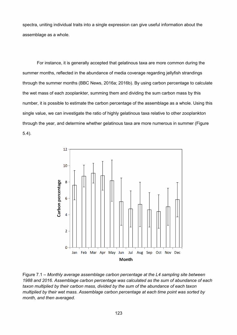
123
spectra, uniting individual traits into a single expression can give useful information about the
assemblage as a whole.
For instance, it is generally accepted that gelatinous taxa are more common during the
summer months, reflected in the abundance of media coverage regarding jellyfish strandings
through the summer months (BBC News, 2016a; 2016b). By using carbon percentage to calculate
the wet mass of each zooplankter, summing them and dividing the sum carbon mass by this
number, it is possible to estimate the carbon percentage of the assemblage as a whole. Using this
single value, we can investigate the ratio of highly gelatinous taxa relative to other zooplankton
through the year, and determine whether gelatinous taxa are more numerous in summer (Figure
5.4).
Figure 7.1 – Monthly average assemblage carbon percentage at the L4 sampling site between1988 and 2016. Assemblage carbon percentage was calculated as the sum of abundance of eachtaxon multiplied by their carbon mass, divided by the sum of the abundance of each taxonmultiplied by their wet mass. Assemblage carbon percentage at each time point was sorted bymonth, and then averaged.

124
According to this index, assemblage carbon percentage is both lowest and most variable in
autumn at L4. This index can be used at different temporal scales to ask different questions, for
instance, when applied to the full L4 time series between 1988 and 2016, there is a trend of
decreasing assemblage carbon percentage over time (Figure 7.2). Further analysis suggests that
this is the result of assemblage carbon percentage decreasing in autumn (Figure 7.3).
Figure 7.2 – Assemblage carbon percentage (averaged by year) at the L4 sampling site recordedweekly between 1988 and 2016. Carbon percentages assigned as described in Chapter 4, df = 28,p = 0.0037, R2 = 0.26, carbon percentage = - 0.0615 year + 129.68. Ctenophores were omitteddue to potential preservation and recording issues.

125
Figure 7.3 – Trends in assemblage carbon percentage at the L4 sampling site between 1988 and2016 in different seasons (winter = Jan, Feb, Mar, spring = Apr, May, Jun, summer = July, Aug,Sep, autumn = Oct, Nov, Dec). Spring carbon percentage = - 0.0457 year + 100.21, p = 0.052, R2
= 0.13. Summer carbon percentage = - 0.0615 year + 128.3, p = 0.104, R2 = 0.095. Autumn carbonpercentage = - 0.0971 year + 199.2, p = 0.007, R2 = 0.24. Winter carbon percentage = 0.0275 year+ 62.422, p = 0.33, R2 = 0.036. As above, ctenophores were omitted due to potential identificationand recording issues.
This plot shows that the trend of decreasing carbon percentage with time is strongest
during autumn. This could help to explain why autumn was also the most variable season in the
above plot of assemblage carbon percentage as a function of month. The intention is not to make
compelling evidence that gelatinous zooplankton are increasing at L4, but rather demonstrate that
carbon percentage can be a valuable way to summarise a zooplankton assemblage. Used in this
way, carbon percentage could be used as a monitoring tool as an alternative to the currently used
Marine Strategy Framework Directive (MSFD) lifeforms approach (Tett et al., 2015) to investigate
the effects of fishing pressure, climate change and increased coastal development on zooplankton
assemblages. While all indices have positive and negative qualities, assemblage carbon
percentage could be particularly useful for comparing across multiple time series where different
species are recorded.

126
7.6 - Closing remarks
Size is seen as the “master” trait because it determines such a wide variety of factors
associated with organismal biology (Andersen, 2016). All physiological and ecological processes
are in some way related to the size of the organism. For most organisms, different metrics of body
size are broadly interchangeable. However; the seemingly exceptional characteristics of highly
gelatinous zooplankton demonstrate that body size is a complex trait that is routinely oversimplified.
Examination of the differences between highly gelatinous taxa and other zooplankton helped to
show that different metrics of body size refer to different characteristics. Carbon mass represents
metabolic body size, the amount of an organism that is actively involved in physiological processes
such as respiration and excretion. Wet mass represents the effective influence of an organism, the
amount of the surrounding environment that interacts with the organism at a given time. Wet mass
also dictates the size of an organism relative to other organisms, a critical factor in determining
food webs. Viewed this way, wet mass can be considered as an “ecological body size”.
The unique physical characteristics of the marine environment allow zooplankton to
decouple these two metrics of body size, such that a single size metric is insufficient to fully define
the range of characteristics commonly associated with body size. This decoupling allows
organisms to adopt combinations of metabolic and ecological body size that otherwise would not
be possible. This can have profound effects on organismal energy budgets and even population
dynamics.
While previous studies have categorically separated jellyfish from other zooplankton, this
thesis has endeavoured to show that the difference is a quantitative one based on these different
metrics of body size. Furthermore, this thesis has demonstrated some of the ways that this can
impact organismal energy budgets irrespective of phylogenetic affiliation, and has provided
reasons why a lowered carbon percentage is seen in such a wide range of phyla. This approach of
adopting carbon percentage as continuous trait to describe the decoupling of metabolic and
127
ecological body size can form a significant step toward a comprehensive picture of how taxa
function and interact in the plankton. Using this information, we can better understand the
differences and similarities between zooplanktonic taxa, and better predict how they might respond
to our changing oceans.
128
References
Acuña, J.L. (2001) Pelagic tunicates: Why gelatinous? American Naturalist 158 100-106.
Acuña, J.L., Lopez-Urrutia, A. and Colin, S. (2011) Faking giants: The evolution of high prey
clearance rates in jellyfishes. Science 333 1627-1629.
Addad, S., Exposito, J. Y., Faye, C., Ricard-Blum, S., and Lethias, C. (2011) Isolation,
characterization and biological evaluation of jellyfish collagen for use in biomedical
applications. Marine Drugs 9 967-983.
Alexander, R.M. (1990) Size, speed and buoyancy adaptations in aquatic animals. American
Zoologist 30 189-196.
Alldredge, A.L. (1984) The quantitative significance of gelatinous zooplankton as pelagic
consumers. In Flows of energy and materials in marine ecosystems (pp. 407-433). Springer US.
Alldredge, A.L. and Madin, L.P. (1982) Pelagic tunicates: unique herbivores in the marine plankton.
Bioscience 32 655-663.
Andersen, K. H., Berge, T., Gonçalves, R.J., Hartvig, M., Heuschele, J., Hylander, S. and Olsson,
K. (2016) Characteristic sizes of life in the oceans, from bacteria to whales. Annual Review of
Marine Science 8 217-241.
Andersen, K.H, Aksnes, D.L., Berge, T., Fiksen, Ø., and Visser, A. (2015a) Modelling emergent
trophic strategies in plankton. Journal of Plankton Research 37 862-868.

129
Andersen, K.H., Berge, T., Goncalves, R.J., Hartvig, M., Heuschele, J., Hylander, S., Jacobsen,
N.S., Lindemann, C. et al. (2015b) Characteristic sizes of life in the oceans, from bacteria to
whales. Annual Review of Marine Science 8 3.1-3.25.
Anderson, J.T., Inouye, D.W., McKinney, A.M., Colautti, R.I. and Mitchell-Olds, T. (2012)
Phenotypic plasticity and adaptive evolution contribute to advancing flowering phenology in
response to climate change. Proceedings of the Royal Society of London B: Biological Sciences,
p.rspb20121051.
Arai, M.N., (2012) A functional biology of Scyphozoa. Springer Science & Business Media.
Atkinson, A., Shreeve, R.S., Hirst, A.G., Rothery, P., Tarling, G.A., Pond, D.W., Korb, R.E., Murphy,
E.J., et al. (2006) Natural growth rates in Antarctic krill (Euphausia superba): II. Predictive models
based on food, temperature, body length, sex and maturity stage. Limnology and Oceanography
51 973-987.
Båmstedt, U., Wild, B. and Martinussen, M. (2001) Significance of food type for growth of ephyrae
Aurelia aurita (Scyphozoa). Marine Biology 139 641-650.
BBC News (2015) Jellyfish at record high, says Marine Conservation Society. [ONLINE] Available
at: http://www.bbc.co.uk/news/uk-england-devon-33988083. [Accessed 27 April 2017].
BBC News (2016a) Stinging jellyfish spotted on Scots beach. [ONLINE] Available at:
http://www.bbc.co.uk/news/uk-scotland-36916594. [Accessed 11 April 2017]
BBC News (2016b) Thousands of jellyfish wash up on Cornish beach. [ONLINE] Available at:
http://www.bbc.co.uk/news/uk-england-cornwall-36793950. [Accessed 11 April 2017]
130
Belsley, D., Kuh, E. and Welsch, R. (1980) Regression diagnostics. Wiley.
Bidigare, R.R. and Biggs, D.C. (1980) The role of sulfate exclusion in buoyancy maintenance by
siphonophores and other oceanic gelatinous zooplankton. Comparative Biochemistry and
Physiology 66A 467-471.
Blackett, M., Lucas, C.H., Harmer, R.A. and Licandro, P. (2015). Population ecology of Muggiaea
atlantica (Cnidaria, Siphonophora) in the Western English Channel. Marine Ecology Progress
Series 535 129-144.
Bone, Q. (ed.) (1998) The biology of pelagic tunicates. Oxford University Press, Oxford.
Brotz, L. and Pauly, D. (2016) Studying jellyfish fisheries: toward accurate national catch reports
and appropriate methods for stock assessments. Jellyfish: Ecology, Distribution Patterns and
Human Interactions. Nova Publishers, Hauppauge, NY.
Brown, J.H., Gillooly, J.F., Allen, A.P., Savage, V.M. and West, G.B. (2004) Toward a metabolic
theory of ecology. Ecology 85 1771-1789.
Burnham, K.P. and Anderson, D.R. (2002) Model selection and multimodel inference: A practical
information-theoretic approach. Springer, New York.
Canepa, A., Fuentes, V., Sabatés, A., Piraino, S., Boero, F. and Gili, J.M. (2014) Pelagia noctiluca
in the Mediterranean Sea. In Jellyfish blooms (pp. 237-266). Springer Netherlands.
Clarke, A. and Peck, L.S. (1991) The physiology of polar marine zooplankton. Polar Research 10
355-370.

131
Clarke, A., Holmes, L.J. and Gore, D.J. (1992) Proximate and elemental composition of gelatinous
zooplankton from the Southern Ocean. Journal of Experimental Marine Biology and Ecology 155
55-68.
Cole, M., Lindeque, P.K., Fileman, E., Halsband, C. and Galloway, T. (2015) The impact of
microplastics on feeding, function and fecundity in the copepod Calanus helgolandicus.
Environmental Science & Technology 49 1130-1137.
Condon, R.H, Duarte, C.M., Pitt, K.A., Robinson, K.L., Lucas, C.H., Sutherland, K.R., Mianzan,
H.W., Bogeberg, M. et al. (2013) Recurrent jellyfish blooms are a consequence of global
oscillations. Proceedings of the National Academy of Sciences U.S.A. 110 1000-1005.
Condon, R.H., Graham, W.M., Duarte, C.M., Pitt, K.A., Lucas, C.H., Haddock, S.H., Sutherland,
K.R., Robinson, K.L., Dawson, M.N., Decker, M.B. and Mills, C.E. (2012) Questioning the rise of
gelatinous zooplankton in the world's oceans. BioScience 62 160-169.
Cross, J., Nimmo-Smith, W.A.M., Hosegood, P.J. and Torres, R. (2015) The role of advection in
the distribution of plankton populations at a moored 1-D coastal observatory. Progress in
Oceanography 137 342-359.
D’Ambra, I., Graham, W.M., Carmichael, R.H. and Hernandez, F.J. (2015) Fish rely on scyphozoan
hosts as a primary food source: evidence from stable isotope analysis. Marine Biology 162 247-
252.
Decker, M.B., Breitburg, D.L. and Purcell, J.E. (2004) Effects of low dissolved oxygen on
zooplankton predation by the ctenophore Mnemiopsis leidyi. Marine Ecology Progress Series 280
163-172.
132
Delannoy, C.M., Houghton, J.D. Fleming, N.E., and Ferguson, H.W. (2011). Mauve Stingers
(Pelagia noctiluca) as carriers of the bacterial fish pathogen Tenacibaculum maritimum.
Aquaculture 311 255-257.
Dong, J., Jiang, L.X., Tan, K. F., Liu, H.Y., Purcell, J. E., Li, P. J., and Ye, C.C. (2009) Stock
enhancement of the edible jellyfish (Rhopilema esculentum Kishinouye) in Liaodong Bay, China: a
review. Hydrobiologia 616 113-118.
Dong, Z., Liu, D. and Keesing, J.K. (2010) Jellyfish blooms in China: dominant species, causes
and consequences. Marine Pollution Bulletin 60 954-963.
Doyle, T. K., De Haas, H., Cotton, D., Dorschel, B., Cummins, V., Houghton, J. D., and Hays, G.C.
(2008). Widespread occurrence of the jellyfish Pelagia noctiluca in Irish coastal and shelf waters.
Journal of Plankton Research 30 963-968.
Duarte, C. M., Pitt, K. A., Lucas, C. H., Purcell, J. E., Uye, S. I., Robinson, K., and Madin, L. (2013)
Is global ocean sprawl a cause of jellyfish blooms? Frontiers in Ecology and the Environment 11
91-97.
Dunn, C.W., Leys, S.P. and Haddock, S.H. (2015) The hidden biology of sponges and ctenophores.
Trends in Ecology & Evolution 30 282-291.
Dunn, C.W., Pugh, P.R. and Haddock, S.H. (2005) Molecular phylogenetics of the siphonophora
(Cnidaria), with implications for the evolution of functional specialization. Systematic Biology 54
916-935.
Edwards, M. and Richardson, A.J. (2004) Impact of climate change on marine pelagic phenology
and trophic mismatch. Nature 430 881.
133
Elliott, D.T., Pierson, J.J. and Roman, M.R. (2012) Relationship between environmental conditions
and zooplankton community structure during summer hypoxia in the northern Gulf of Mexico.
Journal of Plankton Research 34 602-613.
Eloire, D., Somerfield, P.J., Conway, D.V.P., Halsband-Lenk, C., Harris, R. and Bonnet, D. (2010)
Temporal variability and community composition of zooplankton at station L4 in the Western
Channel: 20 years of sampling. Journal of Plankton Research 32 657–679.
Everett, J.D., Baird, M.E., Buchanan, P., Bulman, C., Davies, C., Downie, R., Griffiths, C.,
Heneghan, R., Kloser, R., Laiolo, L. and Lara Lopez, A. (2017) Modelling what we sample and
sampling what we model: challenges for zooplankton model assessment. Frontiers in Marine
Science 4 77.
FAO (1999) Fisheries, Aquaculture Information, Statistics Service FishStatPlus.
Fenner, P.J. and Hadok, J.C. (2002) Fatal envenomation by jellyfish causing Irukandji syndrome.
Medical Journal of Australia 177 362-363.
Finenko, G.A., Kideys, A.E., Anninsky, B.E., Shiganova, T.A., Roohi, A., Tabari, M.R., Rostami, H.
and Bagheri, S. (2006) Invasive ctenophore Mnemiopsis leidyi in the Caspian Sea: feeding,
respiration, reproduction and predatory impact on the zooplankton community. Marine Ecology
Progress Series 314 171-185.
Flynn, K.J. and Mitra, A. (2009) Building the “perfect beast”: modelling mixotrophic plankton.
Journal of Plankton Research 31 965-992.
134
Flynn, K.J., Stoecker, D.K., Mitra, A., Raven, J.A., Glibert, P.M., Hansen, P.J., Granéli, E. and
Burkholder, J.M. (2012) Misuse of the phytoplankton–zooplankton dichotomy: the need to assign
organisms as mixotrophs within plankton functional types. Journal of Plankton Research 35 3-11.
Fosså, J.H. (1992). Mass occurrence of Periphylla periphylla (Scyphozoa, Coronatae) in a
Norwegian fjord. Sarsia 77 237-251.
Fossette, S., Gleiss, A.C., Chalumeau, J., Bastian, T., Armstrong, C.D., Vandenabeele, S.,
Karpytchev, M. and Hays, G.C. (2015) Current-oriented swimming by jellyfish and its role in bloom
maintenance. Current Biology 25 342-347.
Frandsen, K. and Riisgard, H. (1997) Size dependent respiration and growth of jellyfish, Aurelia
aurita. Sarsia 82 307-312.
Frandsen, K.T. and Riisgård, H.U., (1997) Size dependent respiration and growth of jellyfish,
Aurelia aurita. Sarsia 82 307-312.
Fraser, J.H. (1970) The ecology of the ctenophore Pleurobrachia pileus in Scottish waters. ICES
Journal of Marine Science 33149-168.
Fuentes, V.L., Angel, D.L., Bayha, K.M., Atienza, D., Edelist, D., Bordehore, C., Gili, J.M. and
Purcell, J.E. (2010) Blooms of the invasive ctenophore, Mnemiopsis leidyi, span the Mediterranean
Sea in 2009. Hydrobiologia 645 23-37.
Fuentes, V.L., Angel, D.L., Bayha, K.M., Atienza, D., Edelist, D., Bordehore, C., and Purcell, J.E.
(2010) Blooms of the invasive ctenophore, Mnemiopsis leidyi, span the Mediterranean Sea in 2009.
Hydrobiologia 645 23-37.
135
Gemmell, B.J., Costello, J.H., Colin, S.P. Stewart, C.J., Dabiri, J.O.,Tafti, D. and Priya, S. (2013)
Passive energy recapture in jellyfish contributes to propulsive advantage over other metazoans.
Proceedings of the National Academy of Sciences USA 110 17904-17909.
Gibbons, M.J. and Richardson, A.J. (2013) Beyond the jellyfish joyride and global oscillations:
advancing jellyfish research. Journal of Plankton Research 35 929-938.
Gillooly, J.F., Brown, J.H., West, G.B., Savage, V.M. and Charnov, E.L. (2002) Effects of size and
temperature on metabolic rate. Science 293 2248-2251.
Glazier, D.S. (2006) The 3/4-power law is not universal: evolution of isometric, ontogenetic
metabolic scaling in pelagic animals. BioScience 56 325-332.
Glazier, D.S., Hirst, A.G. and Atkinson, D. (2015) Shape shifting predicts ontogenetic changes in
metabolic scaling in diverse aquatic invertebrates. Proceedings of the Royal Society of London B:
Biological Sciences 282 20142302.
Graham, W. M., Pagès, F. and Hamner, W. M. (2001) A physical context for gelatinous
zooplankton aggregations: a review. Hydrobiologia 451 199-212.
Haddock, S. H. (2004) A golden age of gelata: past and future research on planktonic ctenophores
and cnidarians. Coelenterate Biology, Springer, Dordrecht.
Hamner, W.M. and Dawson, M.N., (2009) A review and synthesis on the systematics and evolution
of jellyfish blooms: advantageous aggregations and adaptive assemblages. Hydrobiologia 616
161-191.
136
Hamner, W.M., Madin, L.P., Alldredge, A.L., Gilmer, R.W. and Hamner, P.P. (1975) Underwater
observations of gelatinous zooplankton: sampling problems, feeding biology, and behaviour.
Limnology and Oceanography 20 907-917.
Hansen, P.J., Bjørnsen, P.K., and Hansen, B.W. (1997) Zooplankton grazing and growth: scaling
within the 2–2000 μm body size range. Limnology and Oceanography 42 687-704.
Hansson, L.J. (1997) Effect of temperature on growth rate of Aurelia aurita (Cnidaria, Scyphozoa)
from Gullmarsfjorden, Sweden. Marine Ecology Progress Series 161 145-153.
Hansson, L.J. and Norrman, B. (1995) Release of dissolved organic carbon (DOC) by the
scyphozoan jellyfish Aurelia aurita and its potential influence on the production of planktonic
bacteria. Marine Biology 121 527-532.
Haraldsson, M., Tönnesson, K., Tiselius, P., Thingstad, T.F. and Aksnes, D.L. (2012) Relationship
between fish and jellyfish as a function of eutrophication and water clarity. Marine Ecology
Progress Series 471 73-85.
Harbison, G.R. (1992) The gelatinous inhabitants of the ocean interior. Oceanus 35 18-23.
Harbison, G.R., Biggs, D.C. and Madin, L.P. (1977). The associations of Amphipoda Hyperiidea
with gelatinous zooplankton—II. Associations with Cnidaria, Ctenophora and Radiolaria. Deep Sea
Research 24 465-488.
Harris, R. (2010) The L4 time series: the first 20 years. Journal of Plankton Research 32 577–583.
137
Harris, R.P., Irigoien, X., Head, R.N., Rey, C., Hygum, B.H., Hansen, B.W., Niehoff, B., Meyer-
Harms, B. and Carlotti, F., (2000) Feeding, growth and reproduction in the genus Calanus. ICES
Journal of Marine Science 57 1708-1726.
Harrison, N.M. (1984) Predation on jellyfish and their associates by seabirds. Limnology and
Oceanography 29 1335-1337.
Hébert, M-P., Beisner, B. E. and Maranger, R. (2017) Linking zooplankton community structure to
ecosystem functioning: towards an effect-trait framework. Journal of Plankton Research 39 3-12
Hendrickx, J. (2012). perturb: Tools for evaluating collinearity. R package version 2.05.
http://CRAN.R-project.org/package=perturb
Hirst, A.G. (2012) Intra-specific scaling of mass to length in pelagic animals: ontogenetic shape
change and its implications. Limnology and Oceanography 57 1579-1590.
Hirst, A.G. and Forster, J. (2013) When growth models are not universal: evidence from marine
invertebrates. Proceedings of the Royal Society of London B: Biological Sciences 280 20131546.
Hirst, A.G., Roff, J.C. and Lampitt, R.S. (2003) A synthesis of growth rates in marine epipelagic
invertebrate zooplankton. Advances in Marine Biology 44 1-142.
Hiscock, K., Earll, B. (2015) South West Marine Ecosystems in 2015. [ONLINE] Available at:
http://swmecosystems.co.uk/wp-content/uploads/2017/03/SWME-2015-
collated_reports_FINAL_December.doc [Accessed 12 May 2017]
Hopcroft, R.R. and Roff, J.C. (1995) Zooplankton growth rates: extraordinary production by the
larvacean Oikopleura dioica in tropical waters. Journal of Plankton Research 17 205-220.
138
Hopcroft, R.R., and Roff, J.C., (1995). Zooplankton growth rates: extraordinary production by the
larvacean Oikopleura dioica in tropical waters. Journal of Plankton Research 17 205-220.
Hosia, A., and Båmstedt, U. (2007). Seasonal changes in the gelatinous zooplankton community
and hydromedusa abundances in Korsfjord and Fanafjord, Western Norway. Marine Ecology
Progress Series 351 113-127.
Houghton, J.D., Doyle, T.K., Wilson, M.W., Davenport, J. and Hays, G.C. (2006) Jellyfish
aggregations and leatherback turtle foraging patterns in a temperate coastal environment. Ecology
87 1967-1972.
Ikeda, T. (2013) Synthesis towards a global-bathymetric model of metabolism and chemical
composition of mysid crustaceans. Journal of Experimental Marine Biology and Ecology 445 79-87.
Ikeda, T. (2014) Synthesis toward a global model of metabolism and chemical composition of
medusae and ctenophores. Journal of Experimental Marine Biology and Ecology 456 50-64.
Ikeda, T. and Takahashi, T. (2012) Synthesis towards a global-bathymetric model of metabolism
and chemical composition of marine pelagic chaetognaths. Journal of Experimental Marine Biology
and Ecology 424 78-88.
Jaspers, C., Haraldsson, M., Bolte, S., Reusch, T.B., Thygesen, U.H. and Kiørboe, T. (2012)
Ctenophore population recruits entirely through larval reproduction in the central Baltic Sea.
Biology Letters p.rsbl20120163.
Kawahara, M., Ohtsu, K. and Uye, S.I. (2013) Bloom or non-bloom in the giant jellyfish
Nemopilema nomurai (Scyphozoa: Rhizostomeae): roles of dormant podocysts. Journal of
Plankton Research 35 213-217.
139
Kawahara, M., Uye, S.I., Ohtsu, K. and Iizumi, H. (2006) Unusual population explosion of the giant
jellyfish Nemopilema nomurai (Scyphozoa: Rhizostomeae) in East Asian waters. Marine Ecology
Progress Series 307 161-173.
Kenitz, K.M., Visser, A.W., Mariani, P. and Andersen, K.H. (2017) Seasonal succession in
zooplankton feeding traits reveals trophic trait coupling. Limnology and Oceanography DOI:
10.1002/lno.10494
Kils, U. (1981) The swimming behavior, swimming performance and energy balance of Antarctic
krill, Euphausia superba (No. 3). SCAR and SCOR, Scott Polar Research Institute.
Kim, S. W., and Onbé, T. (1989). Observations on the biology of the marine cladoceran Podon
schmackeri. Journal of Crustacean Biology 9 54-59.
King, K.R., Hollibaugh, J.T., and Azam, F. (1980). Predator-prey interactions between the
larvacean Oikopleura dioica and bacterioplankton in enclosed water columns. Marine Biology 56
49-57.
Kiørboe, T. (2011) How zooplankton feed: mechanisms, traits and trade‐offs. Biological Reviews
86 311-339.
Kiørboe, T. (2013) Zooplankton body composition. Limnology and Oceanography 58 1843-1850.
Kiørboe, T. and Hirst, A.G. (2014) Shifts in mass scaling of respiration, feeding, and growth rates
across life-form transitions in marine pelagic organisms. The American Naturalist 183 118-130.
Kleiber, M. (1932) Body size and metabolism. Hilgardia 6 315-332
140
Kooijman, S.A.L.M. (2010) Dynamic energy budget theory for metabolic organisation. Cambridge
University Press, Cambridge.
Kremer, P. and Reeve, M. (1989) Growth dynamics of a ctenophore (Mnemiopsis) in relation to
variable food supply. II Carbon budgets and growth model. Journal of Plankton Research 11 553-
574.
Lalli, C.M. and Gilmer, R.W. (1989) Pelagic snails: the biology of holoplanktonic gastropod
mollusks. Stanford University Press.
Larimer, J.L. and Ashby, E.A. (1962) Float gases, gas secretion and tissue respiration in the
Portuguese man‐of‐war, Physalia. Journal of Cellular Physiology 60 41-47.
Larson, R.J. (1987) Respiration and carbon turnover rates of medusae from the NE Pacific.
Comparative Biochemistry and Physiology Part A: Physiology 87 93-100.
Lebrato, M., Pitt, K.A., Sweetman, A.K., Jones, D.O., Cartes, J.E., Oschlies, A., Condon, R.H.,
Molinero, J.C., Adler, L., Gaillard, C. and Lloris, D. (2012) Jelly-falls historic and recent
observations: a review to drive future research directions. Hydrobiologia 690 227-245.
Libralato, S., Christensen, V. and Pauly, D. (2006) A method for identifying keystone species in
food web models. Ecological Modelling 195 153-171.
Licandro, P., Conway, D.V.P., Yahia, M.D., De Puelles, M.F., Gasparini, S., Hecq, J.H. and Kirby,
R.R. (2010). A blooming jellyfish in the northeast Atlantic and Mediterranean. Biology Letters
rsbl20100150.
141
Litchman, E., Ohman, M.D. and Kiørboe, T. (2013) Trait-based approaches to zooplankton
communities. Journal of Plankton Research 35 473-484.
Little, W.S. and Copley, N.J. (2003) Silhouette DIGITIZER Version 1.0 Users Guide. Woods Hole
Technical Report.
Lucas C.H. and Dawson M.N. (2014) What are jellyfishes and thaliaceans and why do they bloom?
In: Pitt, K.A. and Lucas, C.H. (eds) Jellyfish blooms (p 9−44). Springer, Dordrecht.
Lucas, C.H., Pitt, K.A., Purcell, J.E., Lebrato, M. and Condon, R.H. (2011) What's in a jellyfish?
Proximate and elemental composition and biometric relationships for use in biogeochemical
studies. Ecology 92 1704-1704.
Luo, J.Y., Grassian, B., Tang, D., Irisson, J.O., Greer, A.T., Guigand, C.M., McClatchie, S. and
Cowen, R.K. (2014) Environmental drivers of the fine-scale distribution of a gelatinous zooplankton
community across a mesoscale front. Marine Ecology Progress Series 510 129-149.
Lynam, C.P. and Brierley, A.S. (2007) Enhanced survival of 0-group gadoid fish under jellyfish
umbrellas. Marine Biology 150 1397-1401.
Lynam, C.P., Gibbons, M.J., Axelsen, B.E., Sparks, C.A., Coetzee, J., Heywood, B.G. and Brierley,
A.S. (2006) Jellyfish overtake fish in a heavily fished ecosystem. Current Biology 16 492.
Lynam, C.P., Heath, M.R., Hay, S.J. and Brierley, A.S. (2005) Evidence for impacts by jellyfish on
North Sea herring recruitment. Marine Ecology Progress Series 298 157-167.
Mackas, D.L., Greve, W., Edwards, M., Chiba, S., Tadokoro, K., Eloire, D., Mazzocchi, M.G.,
Batten, S., Richardson, A.J., Johnson, C. and Head, E. (2012) Changing zooplankton seasonality

142
in a changing ocean: comparing time series of zooplankton phenology. Progress in Oceanography
97 31-62.
Mackas, D.L., Greve, W., Edwards, M., Chiba, S., Tadokoro, K., Eloire, D. and Head, E. (2012)
Changing zooplankton seasonality in a changing ocean: Comparing time series of zooplankton
phenology. Progress in Oceanography 97 31-62.
Madin, L.P. (1982) Production, composition and sedimentation of salp fecal pellets in oceanic
waters. Marine Biology 67 39-45.
Marcos-López, M., Mitchell, S.O. and Rodger, H.D (2016) Pathology and mortality associated with
the mauve stinger jellyfish Pelagia noctiluca in farmed Atlantic salmon Salmo salar L. Journal of
Fish Diseases 39 111-115.
Matsumoto, G.I. (1988) A new species of lobate ctenophore, Leucothea pulchra sp. nov., from the
California Bight. Journal of Plankton Research 10 301-311.
Maud, J.L., Atkinson, A., Hirst, A.G., Lindeque, P.K., Widdicombe, C.E., Harmer, R.A., McEvoy, A.
and Cummings, D.G. (2015) How does Calanus helgolandicus maintain its population in a
changing climate? Analysis of a 25-year time series from the English Channel. Progress in
Oceanography 137 513-523.
Milisenda, G., Rosa, S., Fuentes, V.L., Boero, F., Guglielmo, L., Purcell, J.E. and Piraino, S. (2014).
Jellyfish as prey: frequency of predation and selective foraging of Boops boops (Vertebrata,
Actinopterygii) on the mauve stinger Pelagia noctiluca (Cnidaria, Scyphozoa). PLoS One 9
e94600.
143
Miranda, L.S., Morandini, A.C. and Marques, A.C. (2012) Do Staurozoa bloom? A review of
stauromedusan population biology. Hydrobiologia 690 57-67.
Molina-Ramirez, A., Caceres, C., Romero-Romero, S., Bueno, J., Ignacio Gonzalez-Gordillo, J.,
Irigoien, X., Sostres, J., Bode, A., et al. (2015) Functional differences in the allometry of the water,
carbon and nitrogen content of gelatinous organisms. Journal of Plankton Research. 35 989-1000.
Møller, L.F. and Riisgård, H.U. (2007) Feeding, bioenergetics and growth in the common jellyfish
Aurelia aurita and two hydromedusae, Sarsia tubulosa and Aequorea vitrina. Marine Ecology
Progress Series 346 167-177.
Moloney, C.L. and Field, J.G. (1991) The size-based dynamics of plankton food webs. I. A
simulation model of carbon and nitrogen flows. Journal of Plankton Research 13 1003-1038.
Mullin, M.M., and Onbé, T. (1992). Diel reproduction and vertical distributions of the marine
cladocerans, Evadne tergestina and Penilia avirostris, in contrasting coastal environments. Journal
of Plankton Research 14 41-59.
Nissimov, J.I., Napier, J.A., Allen, M.J., Kimmance, S.A. (2015) Intragenus competition between
coccolithoviruses: an insight on how a select few can come to dominate many. Environmental
Microbiology 18 133-145. 10.1111/1462-2920.12902
Oguz, T., Fach, B. and Salihoglu, B. (2008) Invasion dynamics of the alien ctenophore Mnemiopsis
leidyi and its impact on anchovy collapse in the Black Sea. Journal of Plankton Research 30 1385-
1397.
Olesen, N., Frandsen, K. and Riisgard, H.U., (1994) Population dynamics, growth and energetics
of jellyfish Aurelia aurita in a shallow fjord. Marine Ecology Progress Series. 105 9-18.
144
Pauly, D., Graham, W., Libralato, S., Morissette, L., and Palomares, M. D. (2009) Jellyfish in
ecosystems, online databases, and ecosystem models. Hydrobiologia 616 67-85.
Peters, R.H., (ed.) (1983) The ecological implications of body size. Cambridge University Press,
Cambridge.
Pianka, E.R (1970) On r-and K-selection. The American Naturalist 104 592-597.
Pitt, K.A., Duarte, C.M., Lucas, C.H., Sutherland, K.R., Condon, R.H., Mianzan, H., Purcell, J.E.,
Robinson, K.L., et al. (2013) Jellyfish body plans provide allometric advantages beyond low carbon
percentage. PLoS One 8 e72683.
Platt, T., (1985) Structure of the marine ecosystem: its allometric basis. Canadian Bulletin of
Fisheries and Aquatic Sciences 213 55-64.
Pond, D.W., Harris, R.P., Head, R.N. and Harbour, D. (1996) Environmental and nutritional factors
determining seasonal variability in the fecundity and egg viability of Calanus helgolandicus in
coastal waters off Plymouth, U.K. Marine Ecology Progress Series 143 45-63.
Purcell, J.E. (1984) Predation on fish larvae by Physalia physalis, the Portuguese man of war.
Marine Ecology Progress Series 19 189-191.
Purcell, J.E. (2012) Jellyfish and Ctenophora blooms coincide with human proliferations and
environmental perturbations. Annual Review of Marine Science 4 209-235
Purcell, J.E. and Arai, M.N. (2001) Interactions of pelagic cnidarians and ctenophores with fish: a
review. Hydrobiologia 451 27-44.
145
Purcell, J.E., Breitburg, D.L., Decker, M.B., Graham, W.M., Youngbluth, M.J. and Raskoff, K.A.,
(2001) Pelagic cnidarians and ctenophores in low dissolved oxygen environments: a review.
Coastal and Estuarine Studies 58 77-100.
Purcell, J.E., Uye, S.I. and Lo, W.T. (2007) Anthropogenic causes of jellyfish blooms and their
direct consequences for humans: a review. Marine Ecology Progress Series 350 153-174.
Quiñones, J., Monroy, A., Acha, E.M. and Mianzan, H. (2013) Jellyfish bycatch diminishes profit in
an anchovy fishery off Peru. Fisheries Research 139 47-50.
R Core Team (2014) R: A language and environment for statistical computing. R Foundation for
Statistical Computing, Vienna, Austria. http://www.R-project.org/.
Racault, M.F., Le Quéré, C., Buitenhuis, E., Sathyendranath, S. and Platt, T., (2012) Phytoplankton
phenology in the global ocean. Ecological Indicators 14 152-163.
Raskoff, K.A., Purcell, J.E. and Hopcroft, R.R. (2005) Gelatinous zooplankton of the Arctic Ocean:
in situ observations under the ice. Polar Biology 28 207-217.
Raskoff, K.A., Sommer, F.A., Hamner, W.M. and Cross, K.M. (2003) Collection and culture
techniques for gelatinous zooplankton. The Biological Bulletin 204 68-80.
Redfield, A. C. (1934). On the proportions of organic derivatives in sea water and their relation to
the composition of plankton (pp. 176-92). University Press of Liverpool, Liverpool.
Richardson, A.J., Bakun, A., Hays, G.C. and Gibbons, M.J. (2009) The jellyfish joyride: causes,
consequences and management responses to a more gelatinous future. Trends in Ecology &
Evolution 24 312-322.

146
Roberts, R.J. (2001) Miscellaneous non-infectious diseases. Fish Pathology (pp. 367–379), WB
Saunders, London.
Royall, R.M. (1997) Statistical evidence: a likelihood paradigm. New York, NY: Chapman and Hall.
Sappenfield, A.D., Tarhan, L.G. and Droser, M.L. (2016) Earth's oldest jellyfish strandings: a
unique taphonomic window or just another day at the beach? Geological Magazine 2016 1-16.
Schmidt, K., Atkinson, A., Stübing, D., McClelland, J.W., Montoya, J.P. and Voss, M., (2003)
Trophic relationships among Southern Ocean copepods and krill: some uses and limitations of a
stable isotope approach. Limnology and Oceanography 48 277-289.
Seo, H.C., Kube, M., Edvardsen, R.B., Jensen, M.F., Beck, A., Spriet, E., Gorsky, G., Thompson,
E.M., Lehrach, H., Reinhardt, R. and Chourrout, D. (2001) Miniature genome in the marine
chordate Oikopleura dioica. Science 294 2506-2506.
Shiganova, T.A. and Bulgakova, Y.V. (2000) Effects of gelatinous plankton on Black Sea and Sea
of Azov fish and their food resources. ICES Journal of Marine Science 57 641-648.
Smyth, T., Atkinson, A., Widdicombe, S., Frost, M., Allen, I., Fishwick, J., Quieros, A., Sims, D. and
Barange, M. (2015) The Western Channel. Progress in Oceanography 137 335-341
Sousa, T., Domingos, T., Poggiale, J.C. and Kooijman, S.A.L.M., (2010) Dynamic energy budget
theory restores coherence in biology. Philosophical Transactions of the Royal Society of Biology B
365 3413-3428.
Southward, A.J., Langmead, O., Hardman-Mountford, N.J., Aiken, J., Boalch, G.T., Dando, P.R.,
Genner, M.J., Joint, I., Kendall, M.A., Halliday, N.C., Harris, R.P., Leaper, R., Mieszkowska, N.,
147
Pingree, R.D., Richardson, A.J., Sims, D.W., Smith, T., Walne, A.W. and Hawkins, S.J. (2005)
Long-term oceanographic and ecological research in the western English Channel. Advances in
Marine Biology 47 1-105.
Straile, D. (1997) Gross growth efficiencies of protozoan and metazoan zooplankton and their
dependence on food concentration, predator-prey weight ratio, and taxonomic group. Limnology
and Oceanography 42 1375-1385.
Straile, D., (1997) Gross growth efficiencies of protozoan and metazoan zooplankton and their
dependence on food concentration, predator‐prey weight ratio, and taxonomic group. Limnology
and Oceanography 42 1375-1385.
Sullivan, B.K., Suchman, C.L. and Costello, J.H. (1997) Mechanics of prey selection by ephyrae of
the scyphomedusa Aurelia aurita. Marine Biology 130 213-222.
Sullivan, L.J. and Gifford, D.J. (2007) Growth and feeding rates of the newly hatched ctenophore
Mnemiopsis leidyi. Journal of Plankton Research 29 949-965.
Sutherland, K.L., Madin, L.P. and Stocker, R. (2010) Filtration of submicrometer particles by
pelagic tunicates. Proceedings of the National Academy of Sciences USA 107 15129-15134.
Sweetman, A.K. and Chapman, A. (2011) First observations of jelly-falls at the seafloor in a deep-
sea fjord. Deep Sea Research Part I: Oceanographic Research Papers, 58 1206-1211.
Tett, P. (2015) Guide to the PLANKTON INDEX method and software, v. 3.01.
148
Thuesen, E.V., Rutherford, L.D., Brommer, P.L., Garrison, K., Gutowska, M.A. and Towanda, T.
(2005) Intragel oxygen promotes hypoxia tolerance of scyphomedusae. Journal of Experimental
Biology 208 2475-2482.
Troedsson, C., Bouquet, J.M., Aksnes, D.L. and Thompson, E.M. (2002) Resource allocation
between somatic growth and reproductive output in the pelagic chordate Oikopleura dioica allows
opportunistic response to nutritional variation. Marine Ecology Progress Series 243 83-91.
UNESCO (1968) Zooplankton sampling. Monographs on Oceanographic Methodology, Paris.
Uye, S.I. (2008) Blooms of the giant jellyfish Nemopilema nomurai: a threat to the fisheries
sustainability of the East Asian Marginal Seas. Plankton and Benthos Research 3 125-131.
Uye, S.I. (2014) The giant jellyfish Nemopilema nomurai in East Asian marginal seas. In Jellyfish
Blooms (pp. 185-205) ed. Pitt, K.A, Lucas, C.H., Springer, Netherlands.
Verberk, W.C. and Atkinson, D. (2013) Why polar gigantism and Palaeozoic gigantism are not
equivalent: effects of oxygen and temperature on the body size of ectotherms. Functional Ecology
27 1275-1285.
Vidal, J. and Whitledge, T.E. (1982) Rates of metabolism of planktonic crustaceans as related to
body weight and temperature of habitat. Journal of Plankton Research 4 77-84.
Weltzein, F.A., Hemre, G.I., Evjemo, J.O., Olsen, Y. and Fyhn, H.J. (2000) β-Hydroxybutyrate in
developing nauplii of brine shrimp (Artemia franciscana K.) under feeding and non-feeding
conditions. Comparative Biochemistry and Physiology 125B 63-69
149
Wirtz, K. (2012) Who is eating whom? Morphology and feeding type determine the size relation
between planktonic predators and their ideal prey. Marine Ecology Progress Series 445 1-12
Yang, L.H. and Rudolf, V.H.W. (2010) Phenology, ontogeny and the effects of climate change on
the timing of species interactions. Ecology Letters 13 1-10.
You, K., Ma, C., Gao, H., Li, F., Zhang, M., Qiu, Y., and Wang, B. (2007) Research on the jellyfish
(Rhopilema esculentum Kishinouye) and associated aquaculture techniques in China: current
status. Aquaculture International 15 479-488.
Zhao, J., Ramin, M., Cheng, V. and Arhonditsis, G.B. (2008) Plankton community patterns across
a trophic gradient: the role of zooplankton functional groups. Ecological Modelling 213 417-436.
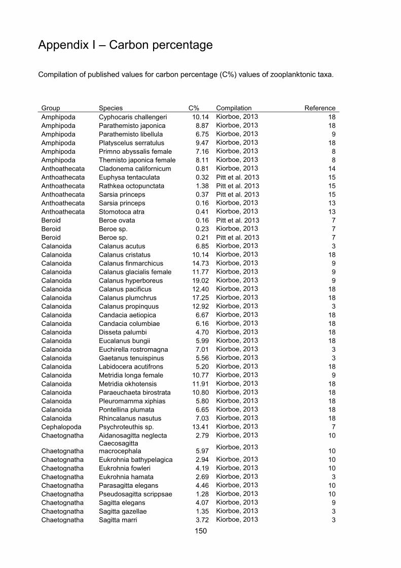
150
Appendix I – Carbon percentage
Compilation of published values for carbon percentage (C%) values of zooplanktonic taxa.
Group Species C% Compilation ReferenceAmphipoda Cyphocaris challengeri 10.14 Kiorboe, 2013 18Amphipoda Parathemisto japonica 8.87 Kiorboe, 2013 18Amphipoda Parathemisto libellula 6.75 Kiorboe, 2013 9Amphipoda Platyscelus serratulus 9.47 Kiorboe, 2013 18Amphipoda Primno abyssalis female 7.16 Kiorboe, 2013 8Amphipoda Themisto japonica female 8.11 Kiorboe, 2013 8Anthoathecata Cladonema californicum 0.81 Kiorboe, 2013 14Anthoathecata Euphysa tentaculata 0.32 Pitt et al. 2013 15Anthoathecata Rathkea octopunctata 1.38 Pitt et al. 2013 15Anthoathecata Sarsia princeps 0.37 Pitt et al. 2013 15Anthoathecata Sarsia princeps 0.16 Kiorboe, 2013 13Anthoathecata Stomotoca atra 0.41 Kiorboe, 2013 13Beroid Beroe ovata 0.16 Pitt et al. 2013 7Beroid Beroe sp. 0.23 Kiorboe, 2013 7Beroid Beroe sp. 0.21 Pitt et al. 2013 7Calanoida Calanus acutus 6.85 Kiorboe, 2013 3Calanoida Calanus cristatus 10.14 Kiorboe, 2013 18Calanoida Calanus finmarchicus 14.73 Kiorboe, 2013 9Calanoida Calanus glacialis female 11.77 Kiorboe, 2013 9Calanoida Calanus hyperboreus 19.02 Kiorboe, 2013 9Calanoida Calanus pacificus 12.40 Kiorboe, 2013 18Calanoida Calanus plumchrus 17.25 Kiorboe, 2013 18Calanoida Calanus propinquus 12.92 Kiorboe, 2013 3Calanoida Candacia aetiopica 6.67 Kiorboe, 2013 18Calanoida Candacia columbiae 6.16 Kiorboe, 2013 18Calanoida Disseta palumbi 4.70 Kiorboe, 2013 18Calanoida Eucalanus bungii 5.99 Kiorboe, 2013 18Calanoida Euchirella rostromagna 7.01 Kiorboe, 2013 3Calanoida Gaetanus tenuispinus 5.56 Kiorboe, 2013 3Calanoida Labidocera acutifrons 5.20 Kiorboe, 2013 18Calanoida Metridia longa female 10.77 Kiorboe, 2013 9Calanoida Metridia okhotensis 11.91 Kiorboe, 2013 18Calanoida Paraeuchaeta birostrata 10.80 Kiorboe, 2013 18Calanoida Pleuromamma xiphias 5.80 Kiorboe, 2013 18Calanoida Pontellina plumata 6.65 Kiorboe, 2013 18Calanoida Rhincalanus nasutus 7.03 Kiorboe, 2013 18Cephalopoda Psychroteuthis sp. 13.41 Kiorboe, 2013 7Chaetognatha Aidanosagitta neglecta 2.79 Kiorboe, 2013 10
ChaetognathaCaecosagittamacrocephala 5.97 Kiorboe, 2013 10
Chaetognatha Eukrohnia bathypelagica 2.94 Kiorboe, 2013 10Chaetognatha Eukrohnia fowleri 4.19 Kiorboe, 2013 10Chaetognatha Eukrohnia hamata 2.69 Kiorboe, 2013 3Chaetognatha Parasagitta elegans 4.46 Kiorboe, 2013 10Chaetognatha Pseudosagitta scrippsae 1.28 Kiorboe, 2013 10Chaetognatha Sagitta elegans 4.07 Kiorboe, 2013 9Chaetognatha Sagitta gazellae 1.35 Kiorboe, 2013 3Chaetognatha Sagitta marri 3.72 Kiorboe, 2013 3
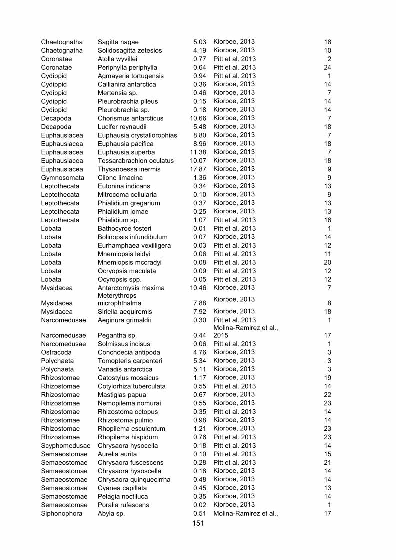
151
Chaetognatha Sagitta nagae 5.03 Kiorboe, 2013 18Chaetognatha Solidosagitta zetesios 4.19 Kiorboe, 2013 10Coronatae Atolla wyvillei 0.77 Pitt et al. 2013 2Coronatae Periphylla periphylla 0.64 Pitt et al. 2013 24Cydippid Agmayeria tortugensis 0.94 Pitt et al. 2013 1Cydippid Callianira antarctica 0.36 Kiorboe, 2013 14Cydippid Mertensia sp. 0.46 Kiorboe, 2013 7Cydippid Pleurobrachia pileus 0.15 Kiorboe, 2013 14Cydippid Pleurobrachia sp. 0.18 Kiorboe, 2013 14Decapoda Chorismus antarcticus 10.66 Kiorboe, 2013 7Decapoda Lucifer reynaudii 5.48 Kiorboe, 2013 18Euphausiacea Euphausia crystallorophias 8.80 Kiorboe, 2013 7Euphausiacea Euphausia pacifica 8.96 Kiorboe, 2013 18Euphausiacea Euphausia superba 11.38 Kiorboe, 2013 7Euphausiacea Tessarabrachion oculatus 10.07 Kiorboe, 2013 18Euphausiacea Thysanoessa inermis 17.87 Kiorboe, 2013 9Gymnosomata Clione limacina 1.36 Kiorboe, 2013 9Leptothecata Eutonina indicans 0.34 Kiorboe, 2013 13Leptothecata Mitrocoma cellularia 0.10 Kiorboe, 2013 9Leptothecata Phialidium gregarium 0.37 Kiorboe, 2013 13Leptothecata Phialidium lomae 0.25 Kiorboe, 2013 13Leptothecata Phialidium sp. 1.07 Pitt et al. 2013 16Lobata Bathocyroe fosteri 0.01 Pitt et al. 2013 1Lobata Bolinopsis infundibulum 0.07 Kiorboe, 2013 14Lobata Eurhamphaea vexilligera 0.03 Pitt et al. 2013 12Lobata Mnemiopsis leidyi 0.06 Pitt et al. 2013 11Lobata Mnemiopsis mccradyi 0.08 Pitt et al. 2013 20Lobata Ocryopsis maculata 0.09 Pitt et al. 2013 12Lobata Ocyropsis spp. 0.05 Pitt et al. 2013 12Mysidacea Antarctomysis maxima 10.46 Kiorboe, 2013 7
MysidaceaMeterythropsmicrophthalma 7.88 Kiorboe, 2013 8
Mysidacea Siriella aequiremis 7.92 Kiorboe, 2013 18Narcomedusae Aeginura grimaldii 0.30 Pitt et al. 2013 1
Narcomedusae Pegantha sp. 0.44Molina-Ramirez et al.,2015 17
Narcomedusae Solmissus incisus 0.06 Pitt et al. 2013 1Ostracoda Conchoecia antipoda 4.76 Kiorboe, 2013 3Polychaeta Tomopteris carpenteri 5.34 Kiorboe, 2013 3Polychaeta Vanadis antarctica 5.11 Kiorboe, 2013 3Rhizostomae Catostylus mosaicus 1.17 Kiorboe, 2013 19Rhizostomae Cotylorhiza tuberculata 0.55 Pitt et al. 2013 14Rhizostomae Mastigias papua 0.67 Kiorboe, 2013 22Rhizostomae Nemopilema nomurai 0.55 Kiorboe, 2013 23Rhizostomae Rhizostoma octopus 0.35 Pitt et al. 2013 14Rhizostomae Rhizostoma pulmo 0.98 Kiorboe, 2013 14Rhizostomae Rhopilema esculentum 1.21 Kiorboe, 2013 23Rhizostomae Rhopilema hispidum 0.76 Pitt et al. 2013 23Scyphomedusae Chrysaora hysocella 0.18 Pitt et al. 2013 14Semaeostomae Aurelia aurita 0.10 Pitt et al. 2013 15Semaeostomae Chrysaora fuscescens 0.28 Pitt et al. 2013 21Semaeostomae Chrysaora hysoscella 0.18 Kiorboe, 2013 14Semaeostomae Chrysaora quinquecirrha 0.48 Kiorboe, 2013 14Semaeostomae Cyanea capillata 0.45 Kiorboe, 2013 13Semaeostomae Pelagia noctiluca 0.35 Kiorboe, 2013 14Semaeostomae Poralia rufescens 0.02 Kiorboe, 2013 1Siphonophora Abyla sp. 0.51 Molina-Ramirez et al., 17
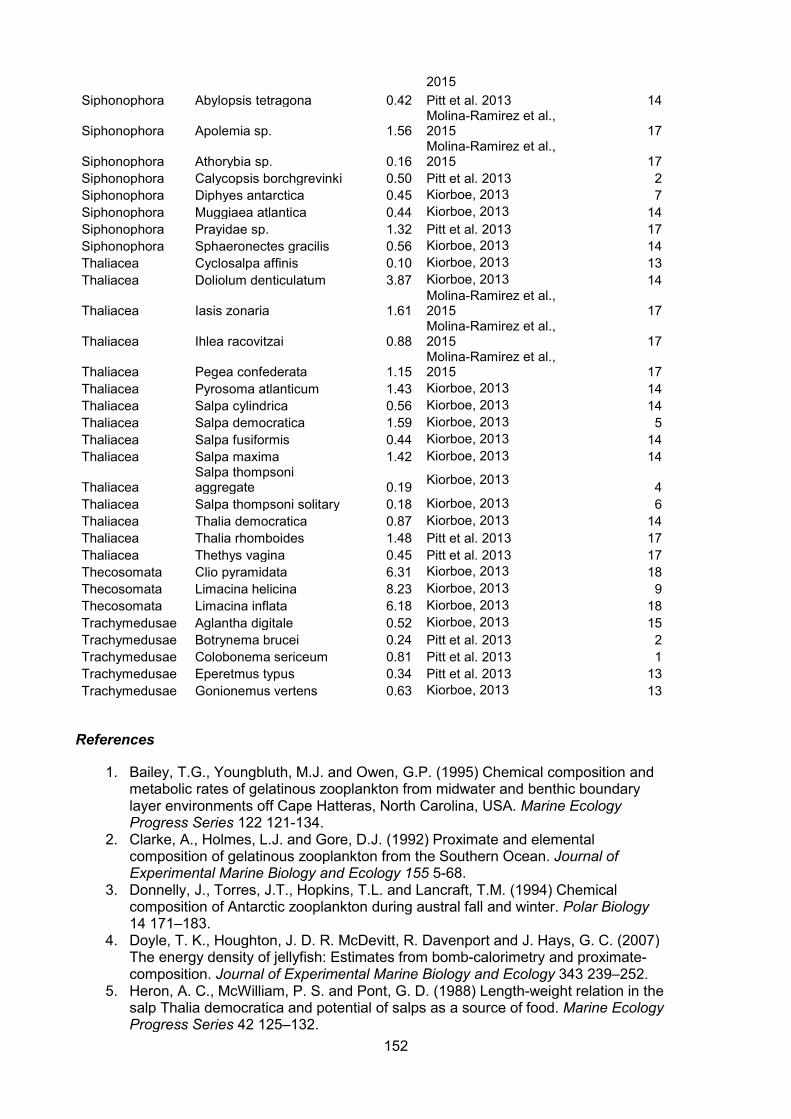
152
2015Siphonophora Abylopsis tetragona 0.42 Pitt et al. 2013 14
Siphonophora Apolemia sp. 1.56Molina-Ramirez et al.,2015 17
Siphonophora Athorybia sp. 0.16Molina-Ramirez et al.,2015 17
Siphonophora Calycopsis borchgrevinki 0.50 Pitt et al. 2013 2Siphonophora Diphyes antarctica 0.45 Kiorboe, 2013 7Siphonophora Muggiaea atlantica 0.44 Kiorboe, 2013 14Siphonophora Prayidae sp. 1.32 Pitt et al. 2013 17Siphonophora Sphaeronectes gracilis 0.56 Kiorboe, 2013 14Thaliacea Cyclosalpa affinis 0.10 Kiorboe, 2013 13Thaliacea Doliolum denticulatum 3.87 Kiorboe, 2013 14
Thaliacea Iasis zonaria 1.61Molina-Ramirez et al.,2015 17
Thaliacea Ihlea racovitzai 0.88Molina-Ramirez et al.,2015 17
Thaliacea Pegea confederata 1.15Molina-Ramirez et al.,2015 17
Thaliacea Pyrosoma atlanticum 1.43 Kiorboe, 2013 14Thaliacea Salpa cylindrica 0.56 Kiorboe, 2013 14Thaliacea Salpa democratica 1.59 Kiorboe, 2013 5Thaliacea Salpa fusiformis 0.44 Kiorboe, 2013 14Thaliacea Salpa maxima 1.42 Kiorboe, 2013 14
ThaliaceaSalpa thompsoniaggregate 0.19 Kiorboe, 2013 4
Thaliacea Salpa thompsoni solitary 0.18 Kiorboe, 2013 6Thaliacea Thalia democratica 0.87 Kiorboe, 2013 14Thaliacea Thalia rhomboides 1.48 Pitt et al. 2013 17Thaliacea Thethys vagina 0.45 Pitt et al. 2013 17Thecosomata Clio pyramidata 6.31 Kiorboe, 2013 18Thecosomata Limacina helicina 8.23 Kiorboe, 2013 9Thecosomata Limacina inflata 6.18 Kiorboe, 2013 18Trachymedusae Aglantha digitale 0.52 Kiorboe, 2013 15Trachymedusae Botrynema brucei 0.24 Pitt et al. 2013 2Trachymedusae Colobonema sericeum 0.81 Pitt et al. 2013 1Trachymedusae Eperetmus typus 0.34 Pitt et al. 2013 13Trachymedusae Gonionemus vertens 0.63 Kiorboe, 2013 13
References
1. Bailey, T.G., Youngbluth, M.J. and Owen, G.P. (1995) Chemical composition andmetabolic rates of gelatinous zooplankton from midwater and benthic boundarylayer environments off Cape Hatteras, North Carolina, USA. Marine EcologyProgress Series 122 121-134.
2. Clarke, A., Holmes, L.J. and Gore, D.J. (1992) Proximate and elementalcomposition of gelatinous zooplankton from the Southern Ocean. Journal ofExperimental Marine Biology and Ecology 155 5-68.
3. Donnelly, J., Torres, J.T., Hopkins, T.L. and Lancraft, T.M. (1994) Chemicalcomposition of Antarctic zooplankton during austral fall and winter. Polar Biology14 171–183.
4. Doyle, T. K., Houghton, J. D. R. McDevitt, R. Davenport and J. Hays, G. C. (2007)The energy density of jellyfish: Estimates from bomb-calorimetry and proximate-composition. Journal of Experimental Marine Biology and Ecology 343 239–252.
5. Heron, A. C., McWilliam, P. S. and Pont, G. D. (1988) Length-weight relation in thesalp Thalia democratica and potential of salps as a source of food. Marine EcologyProgress Series 42 125–132.
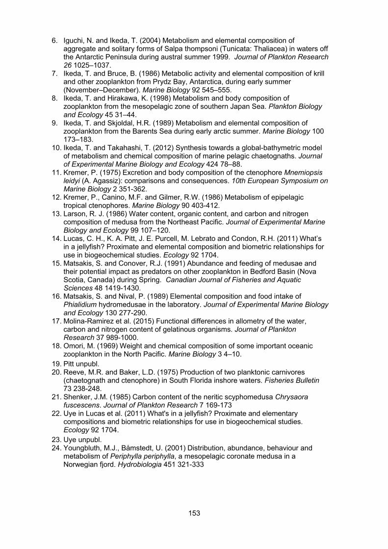
153
6. Iguchi, N. and Ikeda, T. (2004) Metabolism and elemental composition ofaggregate and solitary forms of Salpa thompsoni (Tunicata: Thaliacea) in waters offthe Antarctic Peninsula during austral summer 1999. Journal of Plankton Research26 1025–1037.
7. Ikeda, T. and Bruce, B. (1986) Metabolic activity and elemental composition of krilland other zooplankton from Prydz Bay, Antarctica, during early summer(November–December). Marine Biology 92 545–555.
8. Ikeda, T. and Hirakawa, K. (1998) Metabolism and body composition ofzooplankton from the mesopelagic zone of southern Japan Sea. Plankton Biologyand Ecology 45 31–44.
9. Ikeda, T. and Skjoldal, H.R. (1989) Metabolism and elemental composition ofzooplankton from the Barents Sea during early arctic summer. Marine Biology 100173–183.
10. Ikeda, T. and Takahashi, T. (2012) Synthesis towards a global-bathymetric modelof metabolism and chemical composition of marine pelagic chaetognaths. Journalof Experimental Marine Biology and Ecology 424 78–88.
11. Kremer, P. (1975) Excretion and body composition of the ctenophore Mnemiopsisleidyi (A. Agassiz): comparisons and consequences. 10th European Symposium onMarine Biology 2 351-362.
12. Kremer, P., Canino, M.F. and Gilmer, R.W. (1986) Metabolism of epipelagictropical ctenophores. Marine Biology 90 403-412.
13. Larson, R. J. (1986) Water content, organic content, and carbon and nitrogencomposition of medusa from the Northeast Pacific. Journal of Experimental MarineBiology and Ecology 99 107–120.
14. Lucas, C. H., K. A. Pitt, J. E. Purcell, M. Lebrato and Condon, R.H. (2011) What’sin a jellyfish? Proximate and elemental composition and biometric relationships foruse in biogeochemical studies. Ecology 92 1704.
15. Matsakis, S. and Conover, R.J. (1991) Abundance and feeding of medusae andtheir potential impact as predators on other zooplankton in Bedford Basin (NovaScotia, Canada) during Spring. Canadian Journal of Fisheries and AquaticSciences 48 1419-1430.
16. Matsakis, S. and Nival, P. (1989) Elemental composition and food intake ofPhialidium hydromedusae in the laboratory. Journal of Experimental Marine Biologyand Ecology 130 277-290.
17. Molina-Ramirez et al. (2015) Functional differences in allometry of the water,carbon and nitrogen content of gelatinous organisms. Journal of PlanktonResearch 37 989-1000.
18. Omori, M. (1969) Weight and chemical composition of some important oceaniczooplankton in the North Pacific. Marine Biology 3 4–10.
19. Pitt unpubl.20. Reeve, M.R. and Baker, L.D. (1975) Production of two planktonic carnivores
(chaetognath and ctenophore) in South Florida inshore waters. Fisheries Bulletin73 238-248.
21. Shenker, J.M. (1985) Carbon content of the neritic scyphomedusa Chrysaorafuscescens. Journal of Plankton Research 7 169-173
22. Uye in Lucas et al. (2011) What's in a jellyfish? Proximate and elementarycompositions and biometric relationships for use in biogeochemical studies.Ecology 92 1704.
23. Uye unpubl.24. Youngbluth, M.J., Båmstedt, U. (2001) Distribution, abundance, behaviour and
metabolism of Periphylla periphylla, a mesopelagic coronate medusa in aNorwegian fjord. Hydrobiologia 451 321-333

154
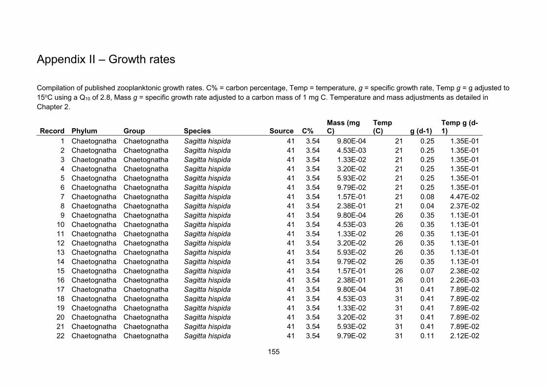
155
Appendix II – Growth rates
Compilation of published zooplanktonic growth rates. C% = carbon percentage, Temp = temperature, g = specific growth rate, Temp g = g adjusted to15oC using a Q10 of 2.8, Mass g = specific growth rate adjusted to a carbon mass of 1 mg C. Temperature and mass adjustments as detailed inChapter 2.
Record Phylum Group Species Source C%Mass (mgC)
Temp(C) g (d-1)
Temp g (d-1)
1 Chaetognatha Chaetognatha Sagitta hispida 41 3.54 9.80E-04 21 0.25 1.35E-012 Chaetognatha Chaetognatha Sagitta hispida 41 3.54 4.53E-03 21 0.25 1.35E-013 Chaetognatha Chaetognatha Sagitta hispida 41 3.54 1.33E-02 21 0.25 1.35E-014 Chaetognatha Chaetognatha Sagitta hispida 41 3.54 3.20E-02 21 0.25 1.35E-015 Chaetognatha Chaetognatha Sagitta hispida 41 3.54 5.93E-02 21 0.25 1.35E-016 Chaetognatha Chaetognatha Sagitta hispida 41 3.54 9.79E-02 21 0.25 1.35E-017 Chaetognatha Chaetognatha Sagitta hispida 41 3.54 1.57E-01 21 0.08 4.47E-028 Chaetognatha Chaetognatha Sagitta hispida 41 3.54 2.38E-01 21 0.04 2.37E-029 Chaetognatha Chaetognatha Sagitta hispida 41 3.54 9.80E-04 26 0.35 1.13E-0110 Chaetognatha Chaetognatha Sagitta hispida 41 3.54 4.53E-03 26 0.35 1.13E-0111 Chaetognatha Chaetognatha Sagitta hispida 41 3.54 1.33E-02 26 0.35 1.13E-0112 Chaetognatha Chaetognatha Sagitta hispida 41 3.54 3.20E-02 26 0.35 1.13E-0113 Chaetognatha Chaetognatha Sagitta hispida 41 3.54 5.93E-02 26 0.35 1.13E-0114 Chaetognatha Chaetognatha Sagitta hispida 41 3.54 9.79E-02 26 0.35 1.13E-0115 Chaetognatha Chaetognatha Sagitta hispida 41 3.54 1.57E-01 26 0.07 2.38E-0216 Chaetognatha Chaetognatha Sagitta hispida 41 3.54 2.38E-01 26 0.01 2.26E-0317 Chaetognatha Chaetognatha Sagitta hispida 41 3.54 9.80E-04 31 0.41 7.89E-0218 Chaetognatha Chaetognatha Sagitta hispida 41 3.54 4.53E-03 31 0.41 7.89E-0219 Chaetognatha Chaetognatha Sagitta hispida 41 3.54 1.33E-02 31 0.41 7.89E-0220 Chaetognatha Chaetognatha Sagitta hispida 41 3.54 3.20E-02 31 0.41 7.89E-0221 Chaetognatha Chaetognatha Sagitta hispida 41 3.54 5.93E-02 31 0.41 7.89E-0222 Chaetognatha Chaetognatha Sagitta hispida 41 3.54 9.79E-02 31 0.11 2.12E-02
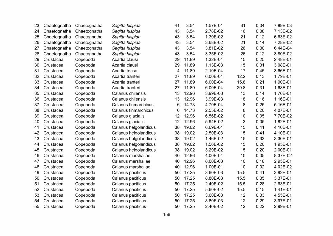
156
23 Chaetognatha Chaetognatha Sagitta hispida 41 3.54 1.57E-01 31 0.04 7.89E-0324 Chaetognatha Chaetognatha Sagitta hispida 43 3.54 2.78E-02 16 0.08 7.13E-0225 Chaetognatha Chaetognatha Sagitta hispida 43 3.54 1.30E-02 21 0.12 6.63E-0226 Chaetognatha Chaetognatha Sagitta hispida 43 3.54 3.68E-02 21 0.14 7.28E-0227 Chaetognatha Chaetognatha Sagitta hispida 43 3.54 3.81E-02 26 0.00 6.44E-0428 Chaetognatha Chaetognatha Sagitta hispida 43 3.54 3.35E-02 26 0.12 3.80E-0229 Crustacea Copepoda Acartia clausi 29 11.89 1.32E-04 15 0.25 2.48E-0130 Crustacea Copepoda Acartia clausi 29 11.89 1.13E-03 15 0.31 3.08E-0131 Crustacea Copepoda Acartia tonsa 4 11.89 2.10E-04 17 0.45 3.66E-0132 Crustacea Copepoda Acartia tranteri 27 11.89 6.00E-04 12.2 0.13 1.79E-0133 Crustacea Copepoda Acartia tranteri 27 11.89 6.00E-04 15.8 0.21 1.90E-0134 Crustacea Copepoda Acartia tranteri 27 11.89 6.00E-04 20.8 0.31 1.68E-0135 Crustacea Copepoda Calanus chilensis 13 12.96 3.99E-03 13 0.14 1.70E-0136 Crustacea Copepoda Calanus chilensis 13 12.96 3.99E-03 18 0.16 1.16E-0137 Crustacea Copepoda Calanus finmarchicus 6 14.73 4.70E-04 8 0.25 5.16E-0138 Crustacea Copepoda Calanus finmarchicus 6 14.73 2.55E-02 8 0.20 4.07E-0139 Crustacea Copepoda Calanus glacialis 12 12.96 6.56E-02 10 0.05 7.70E-0240 Crustacea Copepoda Calanus glacialis 12 12.96 5.94E-02 3 0.05 1.82E-0141 Crustacea Copepoda Calanus helgolandicus 38 19.02 6.69E-04 15 0.41 4.10E-0142 Crustacea Copepoda Calanus helgolandicus 38 19.02 2.50E-03 15 0.41 4.10E-0143 Crustacea Copepoda Calanus helgolandicus 38 19.02 1.46E-02 15 0.33 3.30E-0144 Crustacea Copepoda Calanus helgolandicus 38 19.02 1.56E-02 15 0.20 1.95E-0145 Crustacea Copepoda Calanus helgolandicus 38 19.02 3.29E-02 15 0.20 2.00E-0146 Crustacea Copepoda Calanus marshallae 40 12.96 4.00E-04 10 0.05 8.37E-0247 Crustacea Copepoda Calanus marshallae 40 12.96 8.00E-03 10 0.18 2.95E-0148 Crustacea Copepoda Calanus marshallae 40 12.96 1.00E-01 10 0.02 4.02E-0249 Crustacea Copepoda Calanus pacificus 50 17.25 3.60E-03 15.5 0.41 3.92E-0150 Crustacea Copepoda Calanus pacificus 50 17.25 8.80E-03 15.5 0.35 3.37E-0151 Crustacea Copepoda Calanus pacificus 50 17.25 2.40E-02 15.5 0.28 2.63E-0152 Crustacea Copepoda Calanus pacificus 50 17.25 5.60E-02 15.5 0.15 1.41E-0153 Crustacea Copepoda Calanus pacificus 50 17.25 3.60E-03 12 0.33 4.55E-0154 Crustacea Copepoda Calanus pacificus 50 17.25 8.80E-03 12 0.29 3.97E-0155 Crustacea Copepoda Calanus pacificus 50 17.25 2.40E-02 12 0.22 2.99E-01
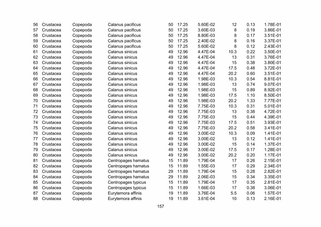
157
56 Crustacea Copepoda Calanus pacificus 50 17.25 5.60E-02 12 0.13 1.78E-0157 Crustacea Copepoda Calanus pacificus 50 17.25 3.60E-03 8 0.19 3.86E-0158 Crustacea Copepoda Calanus pacificus 50 17.25 8.80E-03 8 0.17 3.51E-0159 Crustacea Copepoda Calanus pacificus 50 17.25 2.40E-02 8 0.16 3.37E-0160 Crustacea Copepoda Calanus pacificus 50 17.25 5.60E-02 8 0.12 2.43E-0161 Crustacea Copepoda Calanus sinicus 49 12.96 4.47E-04 10.3 0.22 3.50E-0162 Crustacea Copepoda Calanus sinicus 49 12.96 4.47E-04 13 0.31 3.76E-0163 Crustacea Copepoda Calanus sinicus 49 12.96 4.47E-04 15 0.38 3.80E-0164 Crustacea Copepoda Calanus sinicus 49 12.96 4.47E-04 17.5 0.48 3.72E-0165 Crustacea Copepoda Calanus sinicus 49 12.96 4.47E-04 20.2 0.60 3.51E-0166 Crustacea Copepoda Calanus sinicus 49 12.96 1.98E-03 10.3 0.54 8.81E-0167 Crustacea Copepoda Calanus sinicus 49 12.96 1.98E-03 13 0.74 9.07E-0168 Crustacea Copepoda Calanus sinicus 49 12.96 1.98E-03 15 0.89 8.92E-0169 Crustacea Copepoda Calanus sinicus 49 12.96 1.98E-03 17.5 1.10 8.50E-0170 Crustacea Copepoda Calanus sinicus 49 12.96 1.98E-03 20.2 1.33 7.77E-0171 Crustacea Copepoda Calanus sinicus 49 12.96 7.75E-03 10.3 0.31 5.01E-0172 Crustacea Copepoda Calanus sinicus 49 12.96 7.75E-03 13 0.38 4.72E-0173 Crustacea Copepoda Calanus sinicus 49 12.96 7.75E-03 15 0.44 4.39E-0174 Crustacea Copepoda Calanus sinicus 49 12.96 7.75E-03 17.5 0.51 3.93E-0175 Crustacea Copepoda Calanus sinicus 49 12.96 7.75E-03 20.2 0.58 3.41E-0176 Crustacea Copepoda Calanus sinicus 49 12.96 3.00E-02 10.3 0.09 1.41E-0177 Crustacea Copepoda Calanus sinicus 49 12.96 3.00E-02 13 0.12 1.41E-0178 Crustacea Copepoda Calanus sinicus 49 12.96 3.00E-02 15 0.14 1.37E-0179 Crustacea Copepoda Calanus sinicus 49 12.96 3.00E-02 17.5 0.17 1.28E-0180 Crustacea Copepoda Calanus sinicus 49 12.96 3.00E-02 20.2 0.20 1.17E-0181 Crustacea Copepoda Centropages hamatus 15 11.89 1.79E-04 17 0.26 2.15E-0182 Crustacea Copepoda Centropages hamatus 15 11.89 1.55E-03 17 0.29 2.34E-0183 Crustacea Copepoda Centropages hamatus 29 11.89 1.79E-04 15 0.28 2.82E-0184 Crustacea Copepoda Centropages hamatus 29 11.89 2.06E-03 15 0.34 3.35E-0185 Crustacea Copepoda Centropages typicus 15 11.89 1.79E-04 17 0.35 2.81E-0186 Crustacea Copepoda Centropages typicus 15 11.89 1.66E-03 17 0.38 3.06E-0187 Crustacea Copepoda Eurytemora affinis 19 11.89 3.76E-04 5.5 0.06 1.57E-0188 Crustacea Copepoda Eurytemora affinis 19 11.89 3.61E-04 10 0.13 2.16E-01
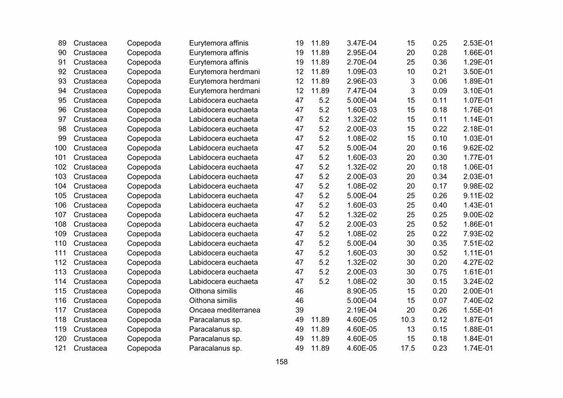
158
89 Crustacea Copepoda Eurytemora affinis 19 11.89 3.47E-04 15 0.25 2.53E-0190 Crustacea Copepoda Eurytemora affinis 19 11.89 2.95E-04 20 0.28 1.66E-0191 Crustacea Copepoda Eurytemora affinis 19 11.89 2.70E-04 25 0.36 1.29E-0192 Crustacea Copepoda Eurytemora herdmani 12 11.89 1.09E-03 10 0.21 3.50E-0193 Crustacea Copepoda Eurytemora herdmani 12 11.89 2.96E-03 3 0.06 1.89E-0194 Crustacea Copepoda Eurytemora herdmani 12 11.89 7.47E-04 3 0.09 3.10E-0195 Crustacea Copepoda Labidocera euchaeta 47 5.2 5.00E-04 15 0.11 1.07E-0196 Crustacea Copepoda Labidocera euchaeta 47 5.2 1.60E-03 15 0.18 1.76E-0197 Crustacea Copepoda Labidocera euchaeta 47 5.2 1.32E-02 15 0.11 1.14E-0198 Crustacea Copepoda Labidocera euchaeta 47 5.2 2.00E-03 15 0.22 2.18E-0199 Crustacea Copepoda Labidocera euchaeta 47 5.2 1.08E-02 15 0.10 1.03E-01100 Crustacea Copepoda Labidocera euchaeta 47 5.2 5.00E-04 20 0.16 9.62E-02101 Crustacea Copepoda Labidocera euchaeta 47 5.2 1.60E-03 20 0.30 1.77E-01102 Crustacea Copepoda Labidocera euchaeta 47 5.2 1.32E-02 20 0.18 1.06E-01103 Crustacea Copepoda Labidocera euchaeta 47 5.2 2.00E-03 20 0.34 2.03E-01104 Crustacea Copepoda Labidocera euchaeta 47 5.2 1.08E-02 20 0.17 9.98E-02105 Crustacea Copepoda Labidocera euchaeta 47 5.2 5.00E-04 25 0.26 9.11E-02106 Crustacea Copepoda Labidocera euchaeta 47 5.2 1.60E-03 25 0.40 1.43E-01107 Crustacea Copepoda Labidocera euchaeta 47 5.2 1.32E-02 25 0.25 9.00E-02108 Crustacea Copepoda Labidocera euchaeta 47 5.2 2.00E-03 25 0.52 1.86E-01109 Crustacea Copepoda Labidocera euchaeta 47 5.2 1.08E-02 25 0.22 7.93E-02110 Crustacea Copepoda Labidocera euchaeta 47 5.2 5.00E-04 30 0.35 7.51E-02111 Crustacea Copepoda Labidocera euchaeta 47 5.2 1.60E-03 30 0.52 1.11E-01112 Crustacea Copepoda Labidocera euchaeta 47 5.2 1.32E-02 30 0.20 4.27E-02113 Crustacea Copepoda Labidocera euchaeta 47 5.2 2.00E-03 30 0.75 1.61E-01114 Crustacea Copepoda Labidocera euchaeta 47 5.2 1.08E-02 30 0.15 3.24E-02115 Crustacea Copepoda Oithona similis 46 8.90E-05 15 0.20 2.00E-01116 Crustacea Copepoda Oithona similis 46 5.00E-04 15 0.07 7.40E-02117 Crustacea Copepoda Oncaea mediterranea 39 2.19E-04 20 0.26 1.55E-01118 Crustacea Copepoda Paracalanus sp. 49 11.89 4.60E-05 10.3 0.12 1.87E-01119 Crustacea Copepoda Paracalanus sp. 49 11.89 4.60E-05 13 0.15 1.88E-01120 Crustacea Copepoda Paracalanus sp. 49 11.89 4.60E-05 15 0.18 1.84E-01121 Crustacea Copepoda Paracalanus sp. 49 11.89 4.60E-05 17.5 0.23 1.74E-01
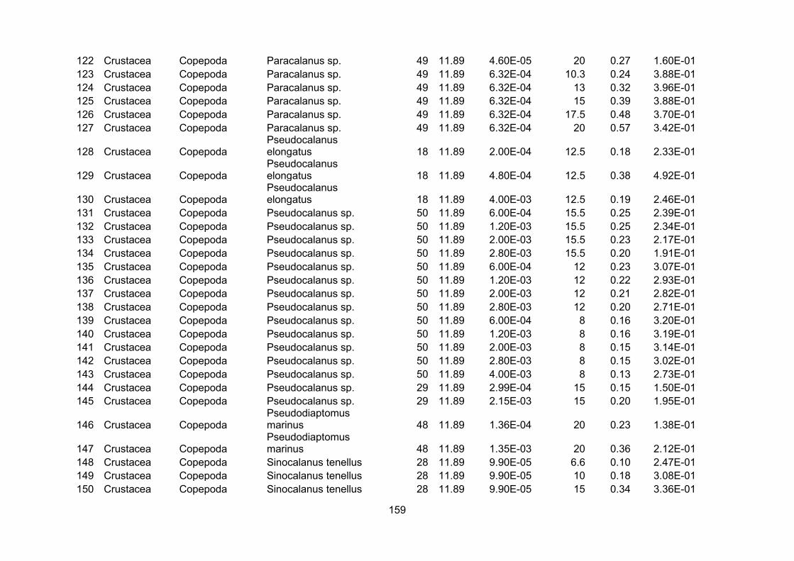
159
122 Crustacea Copepoda Paracalanus sp. 49 11.89 4.60E-05 20 0.27 1.60E-01123 Crustacea Copepoda Paracalanus sp. 49 11.89 6.32E-04 10.3 0.24 3.88E-01124 Crustacea Copepoda Paracalanus sp. 49 11.89 6.32E-04 13 0.32 3.96E-01125 Crustacea Copepoda Paracalanus sp. 49 11.89 6.32E-04 15 0.39 3.88E-01126 Crustacea Copepoda Paracalanus sp. 49 11.89 6.32E-04 17.5 0.48 3.70E-01127 Crustacea Copepoda Paracalanus sp. 49 11.89 6.32E-04 20 0.57 3.42E-01
128 Crustacea CopepodaPseudocalanuselongatus 18 11.89 2.00E-04 12.5 0.18 2.33E-01
129 Crustacea CopepodaPseudocalanuselongatus 18 11.89 4.80E-04 12.5 0.38 4.92E-01
130 Crustacea CopepodaPseudocalanuselongatus 18 11.89 4.00E-03 12.5 0.19 2.46E-01
131 Crustacea Copepoda Pseudocalanus sp. 50 11.89 6.00E-04 15.5 0.25 2.39E-01132 Crustacea Copepoda Pseudocalanus sp. 50 11.89 1.20E-03 15.5 0.25 2.34E-01133 Crustacea Copepoda Pseudocalanus sp. 50 11.89 2.00E-03 15.5 0.23 2.17E-01134 Crustacea Copepoda Pseudocalanus sp. 50 11.89 2.80E-03 15.5 0.20 1.91E-01135 Crustacea Copepoda Pseudocalanus sp. 50 11.89 6.00E-04 12 0.23 3.07E-01136 Crustacea Copepoda Pseudocalanus sp. 50 11.89 1.20E-03 12 0.22 2.93E-01137 Crustacea Copepoda Pseudocalanus sp. 50 11.89 2.00E-03 12 0.21 2.82E-01138 Crustacea Copepoda Pseudocalanus sp. 50 11.89 2.80E-03 12 0.20 2.71E-01139 Crustacea Copepoda Pseudocalanus sp. 50 11.89 6.00E-04 8 0.16 3.20E-01140 Crustacea Copepoda Pseudocalanus sp. 50 11.89 1.20E-03 8 0.16 3.19E-01141 Crustacea Copepoda Pseudocalanus sp. 50 11.89 2.00E-03 8 0.15 3.14E-01142 Crustacea Copepoda Pseudocalanus sp. 50 11.89 2.80E-03 8 0.15 3.02E-01143 Crustacea Copepoda Pseudocalanus sp. 50 11.89 4.00E-03 8 0.13 2.73E-01144 Crustacea Copepoda Pseudocalanus sp. 29 11.89 2.99E-04 15 0.15 1.50E-01145 Crustacea Copepoda Pseudocalanus sp. 29 11.89 2.15E-03 15 0.20 1.95E-01
146 Crustacea CopepodaPseudodiaptomusmarinus 48 11.89 1.36E-04 20 0.23 1.38E-01
147 Crustacea CopepodaPseudodiaptomusmarinus 48 11.89 1.35E-03 20 0.36 2.12E-01
148 Crustacea Copepoda Sinocalanus tenellus 28 11.89 9.90E-05 6.6 0.10 2.47E-01149 Crustacea Copepoda Sinocalanus tenellus 28 11.89 9.90E-05 10 0.18 3.08E-01150 Crustacea Copepoda Sinocalanus tenellus 28 11.89 9.90E-05 15 0.34 3.36E-01

160
151 Crustacea Copepoda Sinocalanus tenellus 28 11.89 9.90E-05 20 0.52 3.13E-01152 Crustacea Copepoda Sinocalanus tenellus 28 11.89 9.90E-05 22 0.61 2.96E-01153 Crustacea Copepoda Sinocalanus tenellus 28 11.89 9.90E-05 28 0.89 2.34E-01154 Crustacea Copepoda Sinocalanus tenellus 28 11.89 1.13E-03 6.6 0.10 2.40E-01155 Crustacea Copepoda Sinocalanus tenellus 28 11.89 1.13E-03 10 0.20 3.33E-01156 Crustacea Copepoda Sinocalanus tenellus 28 11.89 1.13E-03 15 0.40 4.03E-01157 Crustacea Copepoda Sinocalanus tenellus 28 11.89 1.13E-03 20 0.68 4.06E-01158 Crustacea Copepoda Sinocalanus tenellus 28 11.89 1.13E-03 22 0.81 3.94E-01159 Crustacea Copepoda Sinocalanus tenellus 28 11.89 1.13E-03 28 1.28 3.35E-01160 Crustacea Copepoda Temora longicornis 29 11.89 1.79E-04 15 0.26 2.57E-01161 Crustacea Copepoda Temora longicornis 29 11.89 1.68E-03 15 0.34 3.38E-01162 Crustacea Copepoda Temora longicornis 18 11.89 1.30E-04 12.5 0.21 2.72E-01163 Crustacea Copepoda Temora longicornis 18 11.89 1.80E-03 12.5 0.34 4.40E-01164 Crustacea Copepoda Temora longicornis 18 11.89 8.00E-03 12.5 0.31 4.01E-01165 Crustacea Crustacea Calliopius laeviusculus 10 8.42 1.50E-02 8 0.13 2.69E-01166 Crustacea Crustacea Calliopius laeviusculus 10 8.42 3.00E-02 8 0.13 2.57E-01167 Crustacea Crustacea Calliopius laeviusculus 10 8.42 5.00E-02 8 0.12 2.45E-01168 Crustacea Crustacea Calliopius laeviusculus 10 8.42 1.00E-01 8 0.11 2.28E-01169 Crustacea Crustacea Calliopius laeviusculus 10 8.42 1.50E-01 8 0.11 2.16E-01170 Crustacea Crustacea Calliopius laeviusculus 10 8.42 2.00E-01 8 0.10 2.08E-01171 Crustacea Crustacea Calliopius laeviusculus 10 8.42 3.00E-01 8 0.10 1.95E-01172 Crustacea Crustacea Calliopius laeviusculus 10 8.42 5.00E-01 8 0.09 1.75E-01173 Crustacea Crustacea Calliopius laeviusculus 10 8.42 7.50E-01 8 0.08 1.54E-01174 Crustacea Crustacea Calliopius laeviusculus 10 8.42 1.00E+00 8 0.07 1.38E-01175 Crustacea Crustacea Calliopius laeviusculus 10 8.42 1.50E-02 12 0.19 2.63E-01176 Crustacea Crustacea Calliopius laeviusculus 10 8.42 3.00E-02 12 0.18 2.45E-01177 Crustacea Crustacea Calliopius laeviusculus 10 8.42 5.00E-02 12 0.17 2.33E-01178 Crustacea Crustacea Calliopius laeviusculus 10 8.42 1.00E-01 12 0.15 2.10E-01179 Crustacea Crustacea Calliopius laeviusculus 10 8.42 1.50E-01 12 0.15 1.97E-01180 Crustacea Crustacea Calliopius laeviusculus 10 8.42 2.00E-01 12 0.14 1.87E-01181 Crustacea Crustacea Calliopius laeviusculus 10 8.42 3.00E-01 12 0.13 1.70E-01182 Crustacea Crustacea Calliopius laeviusculus 10 8.42 5.00E-01 12 0.11 1.47E-01183 Crustacea Crustacea Calliopius laeviusculus 10 8.42 7.50E-01 12 0.09 1.25E-01
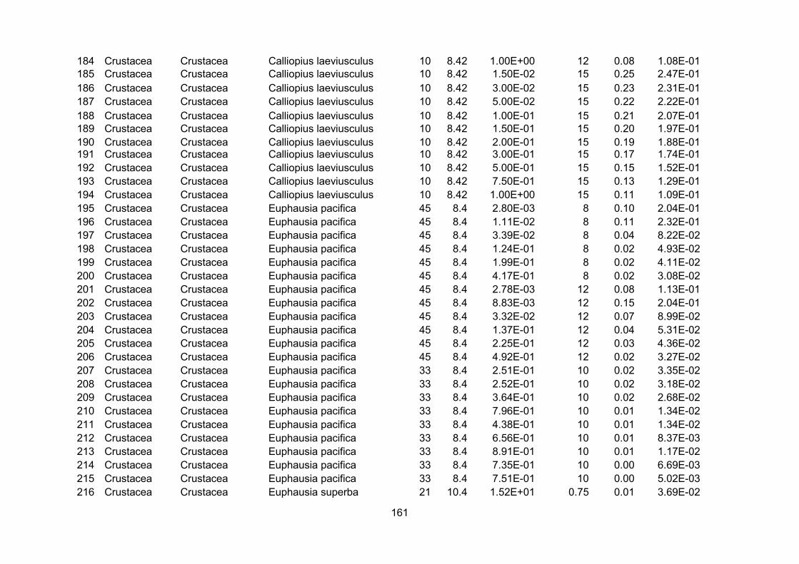
161
184 Crustacea Crustacea Calliopius laeviusculus 10 8.42 1.00E+00 12 0.08 1.08E-01185 Crustacea Crustacea Calliopius laeviusculus 10 8.42 1.50E-02 15 0.25 2.47E-01186 Crustacea Crustacea Calliopius laeviusculus 10 8.42 3.00E-02 15 0.23 2.31E-01187 Crustacea Crustacea Calliopius laeviusculus 10 8.42 5.00E-02 15 0.22 2.22E-01188 Crustacea Crustacea Calliopius laeviusculus 10 8.42 1.00E-01 15 0.21 2.07E-01189 Crustacea Crustacea Calliopius laeviusculus 10 8.42 1.50E-01 15 0.20 1.97E-01190 Crustacea Crustacea Calliopius laeviusculus 10 8.42 2.00E-01 15 0.19 1.88E-01191 Crustacea Crustacea Calliopius laeviusculus 10 8.42 3.00E-01 15 0.17 1.74E-01192 Crustacea Crustacea Calliopius laeviusculus 10 8.42 5.00E-01 15 0.15 1.52E-01193 Crustacea Crustacea Calliopius laeviusculus 10 8.42 7.50E-01 15 0.13 1.29E-01194 Crustacea Crustacea Calliopius laeviusculus 10 8.42 1.00E+00 15 0.11 1.09E-01195 Crustacea Crustacea Euphausia pacifica 45 8.4 2.80E-03 8 0.10 2.04E-01196 Crustacea Crustacea Euphausia pacifica 45 8.4 1.11E-02 8 0.11 2.32E-01197 Crustacea Crustacea Euphausia pacifica 45 8.4 3.39E-02 8 0.04 8.22E-02198 Crustacea Crustacea Euphausia pacifica 45 8.4 1.24E-01 8 0.02 4.93E-02199 Crustacea Crustacea Euphausia pacifica 45 8.4 1.99E-01 8 0.02 4.11E-02200 Crustacea Crustacea Euphausia pacifica 45 8.4 4.17E-01 8 0.02 3.08E-02201 Crustacea Crustacea Euphausia pacifica 45 8.4 2.78E-03 12 0.08 1.13E-01202 Crustacea Crustacea Euphausia pacifica 45 8.4 8.83E-03 12 0.15 2.04E-01203 Crustacea Crustacea Euphausia pacifica 45 8.4 3.32E-02 12 0.07 8.99E-02204 Crustacea Crustacea Euphausia pacifica 45 8.4 1.37E-01 12 0.04 5.31E-02205 Crustacea Crustacea Euphausia pacifica 45 8.4 2.25E-01 12 0.03 4.36E-02206 Crustacea Crustacea Euphausia pacifica 45 8.4 4.92E-01 12 0.02 3.27E-02207 Crustacea Crustacea Euphausia pacifica 33 8.4 2.51E-01 10 0.02 3.35E-02208 Crustacea Crustacea Euphausia pacifica 33 8.4 2.52E-01 10 0.02 3.18E-02209 Crustacea Crustacea Euphausia pacifica 33 8.4 3.64E-01 10 0.02 2.68E-02210 Crustacea Crustacea Euphausia pacifica 33 8.4 7.96E-01 10 0.01 1.34E-02211 Crustacea Crustacea Euphausia pacifica 33 8.4 4.38E-01 10 0.01 1.34E-02212 Crustacea Crustacea Euphausia pacifica 33 8.4 6.56E-01 10 0.01 8.37E-03213 Crustacea Crustacea Euphausia pacifica 33 8.4 8.91E-01 10 0.01 1.17E-02214 Crustacea Crustacea Euphausia pacifica 33 8.4 7.35E-01 10 0.00 6.69E-03215 Crustacea Crustacea Euphausia pacifica 33 8.4 7.51E-01 10 0.00 5.02E-03216 Crustacea Crustacea Euphausia superba 21 10.4 1.52E+01 0.75 0.01 3.69E-02
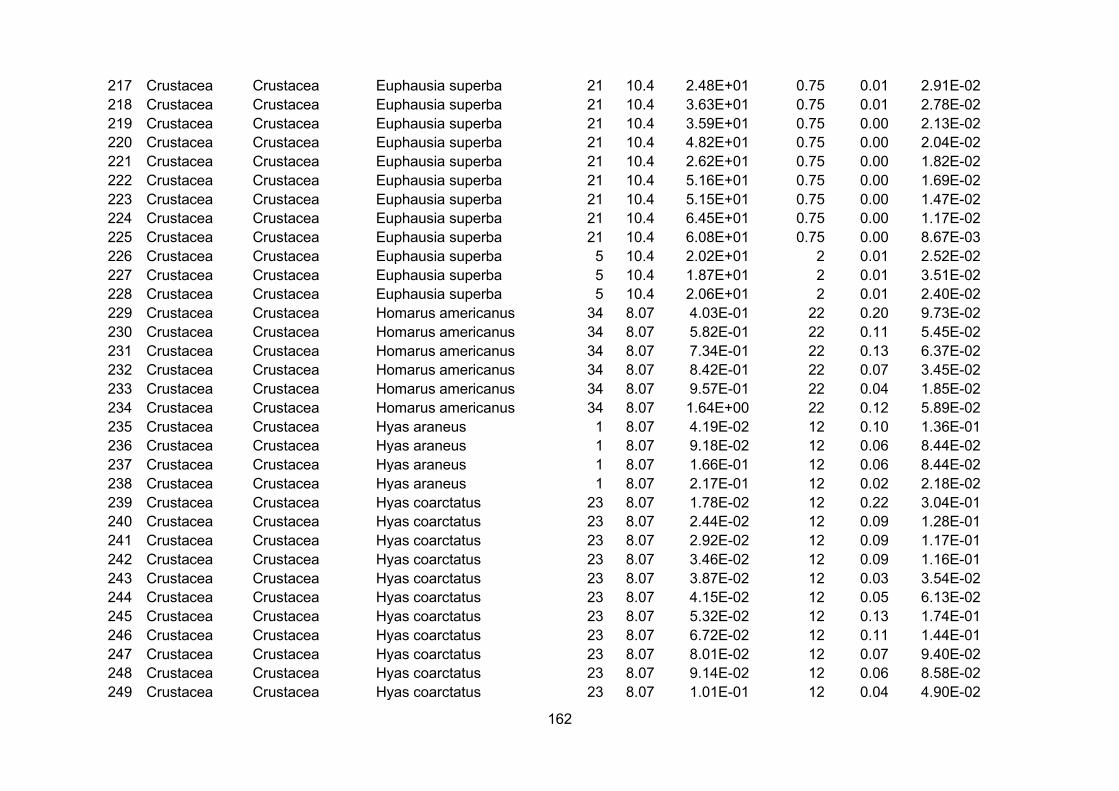
162
217 Crustacea Crustacea Euphausia superba 21 10.4 2.48E+01 0.75 0.01 2.91E-02218 Crustacea Crustacea Euphausia superba 21 10.4 3.63E+01 0.75 0.01 2.78E-02219 Crustacea Crustacea Euphausia superba 21 10.4 3.59E+01 0.75 0.00 2.13E-02220 Crustacea Crustacea Euphausia superba 21 10.4 4.82E+01 0.75 0.00 2.04E-02221 Crustacea Crustacea Euphausia superba 21 10.4 2.62E+01 0.75 0.00 1.82E-02222 Crustacea Crustacea Euphausia superba 21 10.4 5.16E+01 0.75 0.00 1.69E-02223 Crustacea Crustacea Euphausia superba 21 10.4 5.15E+01 0.75 0.00 1.47E-02224 Crustacea Crustacea Euphausia superba 21 10.4 6.45E+01 0.75 0.00 1.17E-02225 Crustacea Crustacea Euphausia superba 21 10.4 6.08E+01 0.75 0.00 8.67E-03226 Crustacea Crustacea Euphausia superba 5 10.4 2.02E+01 2 0.01 2.52E-02227 Crustacea Crustacea Euphausia superba 5 10.4 1.87E+01 2 0.01 3.51E-02228 Crustacea Crustacea Euphausia superba 5 10.4 2.06E+01 2 0.01 2.40E-02229 Crustacea Crustacea Homarus americanus 34 8.07 4.03E-01 22 0.20 9.73E-02230 Crustacea Crustacea Homarus americanus 34 8.07 5.82E-01 22 0.11 5.45E-02231 Crustacea Crustacea Homarus americanus 34 8.07 7.34E-01 22 0.13 6.37E-02232 Crustacea Crustacea Homarus americanus 34 8.07 8.42E-01 22 0.07 3.45E-02233 Crustacea Crustacea Homarus americanus 34 8.07 9.57E-01 22 0.04 1.85E-02234 Crustacea Crustacea Homarus americanus 34 8.07 1.64E+00 22 0.12 5.89E-02235 Crustacea Crustacea Hyas araneus 1 8.07 4.19E-02 12 0.10 1.36E-01236 Crustacea Crustacea Hyas araneus 1 8.07 9.18E-02 12 0.06 8.44E-02237 Crustacea Crustacea Hyas araneus 1 8.07 1.66E-01 12 0.06 8.44E-02238 Crustacea Crustacea Hyas araneus 1 8.07 2.17E-01 12 0.02 2.18E-02239 Crustacea Crustacea Hyas coarctatus 23 8.07 1.78E-02 12 0.22 3.04E-01240 Crustacea Crustacea Hyas coarctatus 23 8.07 2.44E-02 12 0.09 1.28E-01241 Crustacea Crustacea Hyas coarctatus 23 8.07 2.92E-02 12 0.09 1.17E-01242 Crustacea Crustacea Hyas coarctatus 23 8.07 3.46E-02 12 0.09 1.16E-01243 Crustacea Crustacea Hyas coarctatus 23 8.07 3.87E-02 12 0.03 3.54E-02244 Crustacea Crustacea Hyas coarctatus 23 8.07 4.15E-02 12 0.05 6.13E-02245 Crustacea Crustacea Hyas coarctatus 23 8.07 5.32E-02 12 0.13 1.74E-01246 Crustacea Crustacea Hyas coarctatus 23 8.07 6.72E-02 12 0.11 1.44E-01247 Crustacea Crustacea Hyas coarctatus 23 8.07 8.01E-02 12 0.07 9.40E-02248 Crustacea Crustacea Hyas coarctatus 23 8.07 9.14E-02 12 0.06 8.58E-02249 Crustacea Crustacea Hyas coarctatus 23 8.07 1.01E-01 12 0.04 4.90E-02
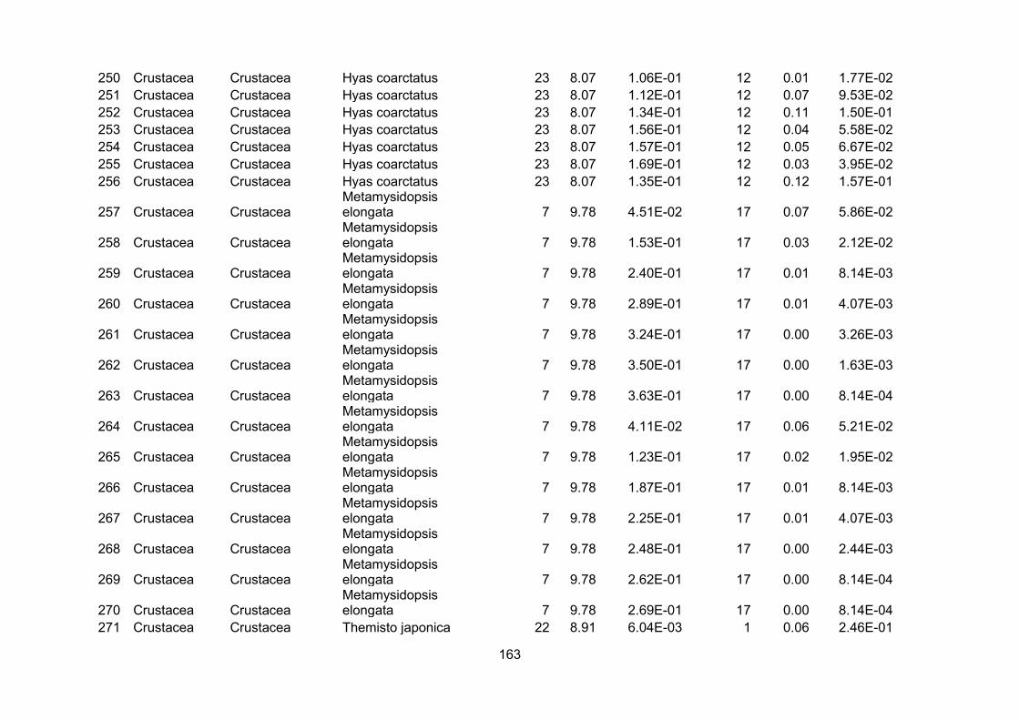
163
250 Crustacea Crustacea Hyas coarctatus 23 8.07 1.06E-01 12 0.01 1.77E-02251 Crustacea Crustacea Hyas coarctatus 23 8.07 1.12E-01 12 0.07 9.53E-02252 Crustacea Crustacea Hyas coarctatus 23 8.07 1.34E-01 12 0.11 1.50E-01253 Crustacea Crustacea Hyas coarctatus 23 8.07 1.56E-01 12 0.04 5.58E-02254 Crustacea Crustacea Hyas coarctatus 23 8.07 1.57E-01 12 0.05 6.67E-02255 Crustacea Crustacea Hyas coarctatus 23 8.07 1.69E-01 12 0.03 3.95E-02256 Crustacea Crustacea Hyas coarctatus 23 8.07 1.35E-01 12 0.12 1.57E-01
257 Crustacea CrustaceaMetamysidopsiselongata 7 9.78 4.51E-02 17 0.07 5.86E-02
258 Crustacea CrustaceaMetamysidopsiselongata 7 9.78 1.53E-01 17 0.03 2.12E-02
259 Crustacea CrustaceaMetamysidopsiselongata 7 9.78 2.40E-01 17 0.01 8.14E-03
260 Crustacea CrustaceaMetamysidopsiselongata 7 9.78 2.89E-01 17 0.01 4.07E-03
261 Crustacea CrustaceaMetamysidopsiselongata 7 9.78 3.24E-01 17 0.00 3.26E-03
262 Crustacea CrustaceaMetamysidopsiselongata 7 9.78 3.50E-01 17 0.00 1.63E-03
263 Crustacea CrustaceaMetamysidopsiselongata 7 9.78 3.63E-01 17 0.00 8.14E-04
264 Crustacea CrustaceaMetamysidopsiselongata 7 9.78 4.11E-02 17 0.06 5.21E-02
265 Crustacea CrustaceaMetamysidopsiselongata 7 9.78 1.23E-01 17 0.02 1.95E-02
266 Crustacea CrustaceaMetamysidopsiselongata 7 9.78 1.87E-01 17 0.01 8.14E-03
267 Crustacea CrustaceaMetamysidopsiselongata 7 9.78 2.25E-01 17 0.01 4.07E-03
268 Crustacea CrustaceaMetamysidopsiselongata 7 9.78 2.48E-01 17 0.00 2.44E-03
269 Crustacea CrustaceaMetamysidopsiselongata 7 9.78 2.62E-01 17 0.00 8.14E-04
270 Crustacea CrustaceaMetamysidopsiselongata 7 9.78 2.69E-01 17 0.00 8.14E-04
271 Crustacea Crustacea Themisto japonica 22 8.91 6.04E-03 1 0.06 2.46E-01
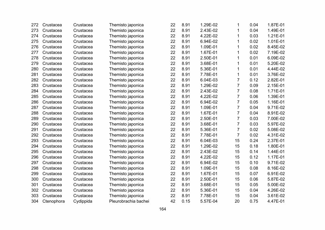
164
272 Crustacea Crustacea Themisto japonica 22 8.91 1.29E-02 1 0.04 1.87E-01273 Crustacea Crustacea Themisto japonica 22 8.91 2.43E-02 1 0.04 1.49E-01274 Crustacea Crustacea Themisto japonica 22 8.91 4.22E-02 1 0.03 1.21E-01275 Crustacea Crustacea Themisto japonica 22 8.91 6.94E-02 1 0.02 1.01E-01276 Crustacea Crustacea Themisto japonica 22 8.91 1.09E-01 1 0.02 8.45E-02277 Crustacea Crustacea Themisto japonica 22 8.91 1.67E-01 1 0.02 7.19E-02278 Crustacea Crustacea Themisto japonica 22 8.91 2.50E-01 1 0.01 6.09E-02279 Crustacea Crustacea Themisto japonica 22 8.91 3.68E-01 1 0.01 5.20E-02280 Crustacea Crustacea Themisto japonica 22 8.91 5.36E-01 1 0.01 4.44E-02281 Crustacea Crustacea Themisto japonica 22 8.91 7.78E-01 1 0.01 3.76E-02282 Crustacea Crustacea Themisto japonica 22 8.91 6.04E-03 7 0.12 2.82E-01283 Crustacea Crustacea Themisto japonica 22 8.91 1.29E-02 7 0.09 2.15E-01284 Crustacea Crustacea Themisto japonica 22 8.91 2.43E-02 7 0.08 1.71E-01285 Crustacea Crustacea Themisto japonica 22 8.91 4.22E-02 7 0.06 1.39E-01286 Crustacea Crustacea Themisto japonica 22 8.91 6.94E-02 7 0.05 1.16E-01287 Crustacea Crustacea Themisto japonica 22 8.91 1.09E-01 7 0.04 9.71E-02288 Crustacea Crustacea Themisto japonica 22 8.91 1.67E-01 7 0.04 8.91E-02289 Crustacea Crustacea Themisto japonica 22 8.91 2.50E-01 7 0.03 7.00E-02290 Crustacea Crustacea Themisto japonica 22 8.91 3.68E-01 7 0.03 5.97E-02291 Crustacea Crustacea Themisto japonica 22 8.91 5.36E-01 7 0.02 5.08E-02292 Crustacea Crustacea Themisto japonica 22 8.91 7.78E-01 7 0.02 4.31E-02293 Crustacea Crustacea Themisto japonica 22 8.91 6.04E-03 15 0.24 2.37E-01294 Crustacea Crustacea Themisto japonica 22 8.91 1.29E-02 15 0.18 1.80E-01295 Crustacea Crustacea Themisto japonica 22 8.91 2.43E-02 15 0.14 1.44E-01296 Crustacea Crustacea Themisto japonica 22 8.91 4.22E-02 15 0.12 1.17E-01297 Crustacea Crustacea Themisto japonica 22 8.91 6.94E-02 15 0.10 9.71E-02298 Crustacea Crustacea Themisto japonica 22 8.91 1.09E-01 15 0.08 8.16E-02299 Crustacea Crustacea Themisto japonica 22 8.91 1.67E-01 15 0.07 6.91E-02300 Crustacea Crustacea Themisto japonica 22 8.91 2.50E-01 15 0.06 5.87E-02301 Crustacea Crustacea Themisto japonica 22 8.91 3.68E-01 15 0.05 5.00E-02302 Crustacea Crustacea Themisto japonica 22 8.91 5.36E-01 15 0.04 4.26E-02303 Crustacea Crustacea Themisto japonica 22 8.91 7.78E-01 15 0.04 3.61E-02304 Ctenophora Cydippida Pleurobrachia bachei 42 0.15 5.57E-04 20 0.75 4.47E-01
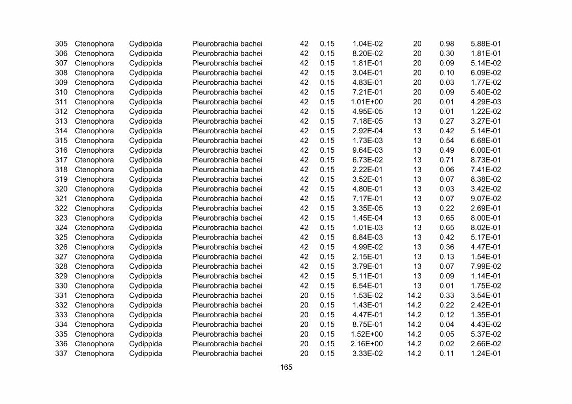
165
305 Ctenophora Cydippida Pleurobrachia bachei 42 0.15 1.04E-02 20 0.98 5.88E-01306 Ctenophora Cydippida Pleurobrachia bachei 42 0.15 8.20E-02 20 0.30 1.81E-01307 Ctenophora Cydippida Pleurobrachia bachei 42 0.15 1.81E-01 20 0.09 5.14E-02308 Ctenophora Cydippida Pleurobrachia bachei 42 0.15 3.04E-01 20 0.10 6.09E-02309 Ctenophora Cydippida Pleurobrachia bachei 42 0.15 4.83E-01 20 0.03 1.77E-02310 Ctenophora Cydippida Pleurobrachia bachei 42 0.15 7.21E-01 20 0.09 5.40E-02311 Ctenophora Cydippida Pleurobrachia bachei 42 0.15 1.01E+00 20 0.01 4.29E-03312 Ctenophora Cydippida Pleurobrachia bachei 42 0.15 4.95E-05 13 0.01 1.22E-02313 Ctenophora Cydippida Pleurobrachia bachei 42 0.15 7.18E-05 13 0.27 3.27E-01314 Ctenophora Cydippida Pleurobrachia bachei 42 0.15 2.92E-04 13 0.42 5.14E-01315 Ctenophora Cydippida Pleurobrachia bachei 42 0.15 1.73E-03 13 0.54 6.68E-01316 Ctenophora Cydippida Pleurobrachia bachei 42 0.15 9.64E-03 13 0.49 6.00E-01317 Ctenophora Cydippida Pleurobrachia bachei 42 0.15 6.73E-02 13 0.71 8.73E-01318 Ctenophora Cydippida Pleurobrachia bachei 42 0.15 2.22E-01 13 0.06 7.41E-02319 Ctenophora Cydippida Pleurobrachia bachei 42 0.15 3.52E-01 13 0.07 8.38E-02320 Ctenophora Cydippida Pleurobrachia bachei 42 0.15 4.80E-01 13 0.03 3.42E-02321 Ctenophora Cydippida Pleurobrachia bachei 42 0.15 7.17E-01 13 0.07 9.07E-02322 Ctenophora Cydippida Pleurobrachia bachei 42 0.15 3.35E-05 13 0.22 2.69E-01323 Ctenophora Cydippida Pleurobrachia bachei 42 0.15 1.45E-04 13 0.65 8.00E-01324 Ctenophora Cydippida Pleurobrachia bachei 42 0.15 1.01E-03 13 0.65 8.02E-01325 Ctenophora Cydippida Pleurobrachia bachei 42 0.15 6.84E-03 13 0.42 5.17E-01326 Ctenophora Cydippida Pleurobrachia bachei 42 0.15 4.99E-02 13 0.36 4.47E-01327 Ctenophora Cydippida Pleurobrachia bachei 42 0.15 2.15E-01 13 0.13 1.54E-01328 Ctenophora Cydippida Pleurobrachia bachei 42 0.15 3.79E-01 13 0.07 7.99E-02329 Ctenophora Cydippida Pleurobrachia bachei 42 0.15 5.11E-01 13 0.09 1.14E-01330 Ctenophora Cydippida Pleurobrachia bachei 42 0.15 6.54E-01 13 0.01 1.75E-02331 Ctenophora Cydippida Pleurobrachia bachei 20 0.15 1.53E-02 14.2 0.33 3.54E-01332 Ctenophora Cydippida Pleurobrachia bachei 20 0.15 1.43E-01 14.2 0.22 2.42E-01333 Ctenophora Cydippida Pleurobrachia bachei 20 0.15 4.47E-01 14.2 0.12 1.35E-01334 Ctenophora Cydippida Pleurobrachia bachei 20 0.15 8.75E-01 14.2 0.04 4.43E-02335 Ctenophora Cydippida Pleurobrachia bachei 20 0.15 1.52E+00 14.2 0.05 5.37E-02336 Ctenophora Cydippida Pleurobrachia bachei 20 0.15 2.16E+00 14.2 0.02 2.66E-02337 Ctenophora Cydippida Pleurobrachia bachei 20 0.15 3.33E-02 14.2 0.11 1.24E-01
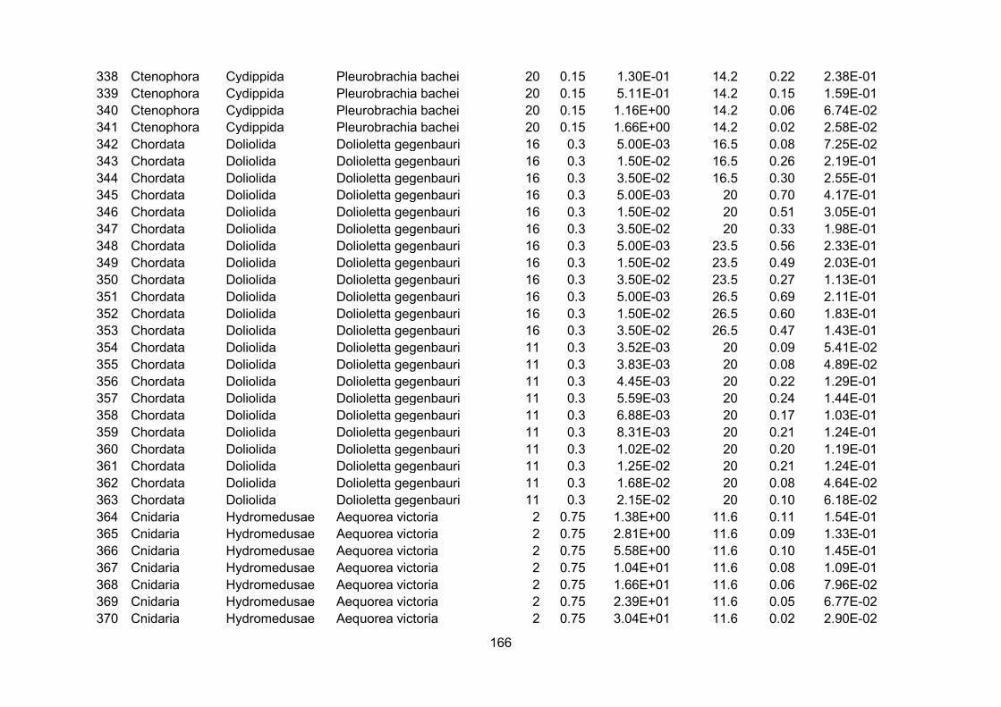
166
338 Ctenophora Cydippida Pleurobrachia bachei 20 0.15 1.30E-01 14.2 0.22 2.38E-01339 Ctenophora Cydippida Pleurobrachia bachei 20 0.15 5.11E-01 14.2 0.15 1.59E-01340 Ctenophora Cydippida Pleurobrachia bachei 20 0.15 1.16E+00 14.2 0.06 6.74E-02341 Ctenophora Cydippida Pleurobrachia bachei 20 0.15 1.66E+00 14.2 0.02 2.58E-02342 Chordata Doliolida Dolioletta gegenbauri 16 0.3 5.00E-03 16.5 0.08 7.25E-02343 Chordata Doliolida Dolioletta gegenbauri 16 0.3 1.50E-02 16.5 0.26 2.19E-01344 Chordata Doliolida Dolioletta gegenbauri 16 0.3 3.50E-02 16.5 0.30 2.55E-01345 Chordata Doliolida Dolioletta gegenbauri 16 0.3 5.00E-03 20 0.70 4.17E-01346 Chordata Doliolida Dolioletta gegenbauri 16 0.3 1.50E-02 20 0.51 3.05E-01347 Chordata Doliolida Dolioletta gegenbauri 16 0.3 3.50E-02 20 0.33 1.98E-01348 Chordata Doliolida Dolioletta gegenbauri 16 0.3 5.00E-03 23.5 0.56 2.33E-01349 Chordata Doliolida Dolioletta gegenbauri 16 0.3 1.50E-02 23.5 0.49 2.03E-01350 Chordata Doliolida Dolioletta gegenbauri 16 0.3 3.50E-02 23.5 0.27 1.13E-01351 Chordata Doliolida Dolioletta gegenbauri 16 0.3 5.00E-03 26.5 0.69 2.11E-01352 Chordata Doliolida Dolioletta gegenbauri 16 0.3 1.50E-02 26.5 0.60 1.83E-01353 Chordata Doliolida Dolioletta gegenbauri 16 0.3 3.50E-02 26.5 0.47 1.43E-01354 Chordata Doliolida Dolioletta gegenbauri 11 0.3 3.52E-03 20 0.09 5.41E-02355 Chordata Doliolida Dolioletta gegenbauri 11 0.3 3.83E-03 20 0.08 4.89E-02356 Chordata Doliolida Dolioletta gegenbauri 11 0.3 4.45E-03 20 0.22 1.29E-01357 Chordata Doliolida Dolioletta gegenbauri 11 0.3 5.59E-03 20 0.24 1.44E-01358 Chordata Doliolida Dolioletta gegenbauri 11 0.3 6.88E-03 20 0.17 1.03E-01359 Chordata Doliolida Dolioletta gegenbauri 11 0.3 8.31E-03 20 0.21 1.24E-01360 Chordata Doliolida Dolioletta gegenbauri 11 0.3 1.02E-02 20 0.20 1.19E-01361 Chordata Doliolida Dolioletta gegenbauri 11 0.3 1.25E-02 20 0.21 1.24E-01362 Chordata Doliolida Dolioletta gegenbauri 11 0.3 1.68E-02 20 0.08 4.64E-02363 Chordata Doliolida Dolioletta gegenbauri 11 0.3 2.15E-02 20 0.10 6.18E-02364 Cnidaria Hydromedusae Aequorea victoria 2 0.75 1.38E+00 11.6 0.11 1.54E-01365 Cnidaria Hydromedusae Aequorea victoria 2 0.75 2.81E+00 11.6 0.09 1.33E-01366 Cnidaria Hydromedusae Aequorea victoria 2 0.75 5.58E+00 11.6 0.10 1.45E-01367 Cnidaria Hydromedusae Aequorea victoria 2 0.75 1.04E+01 11.6 0.08 1.09E-01368 Cnidaria Hydromedusae Aequorea victoria 2 0.75 1.66E+01 11.6 0.06 7.96E-02369 Cnidaria Hydromedusae Aequorea victoria 2 0.75 2.39E+01 11.6 0.05 6.77E-02370 Cnidaria Hydromedusae Aequorea victoria 2 0.75 3.04E+01 11.6 0.02 2.90E-02
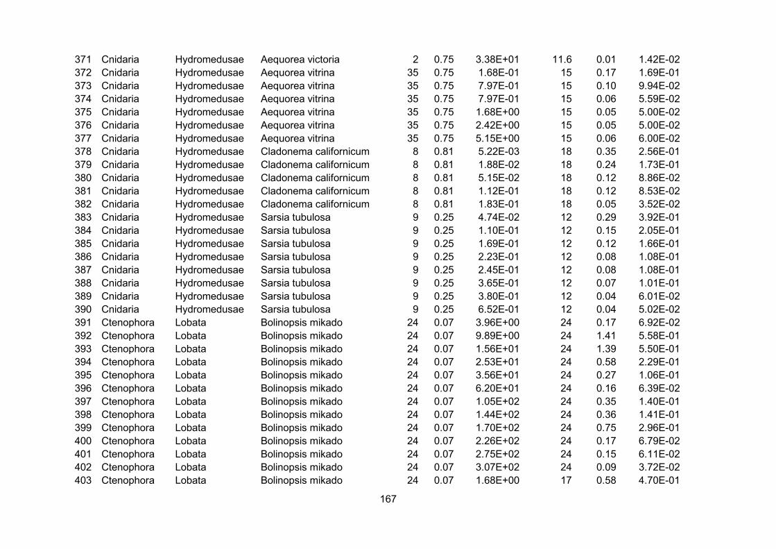
167
371 Cnidaria Hydromedusae Aequorea victoria 2 0.75 3.38E+01 11.6 0.01 1.42E-02372 Cnidaria Hydromedusae Aequorea vitrina 35 0.75 1.68E-01 15 0.17 1.69E-01373 Cnidaria Hydromedusae Aequorea vitrina 35 0.75 7.97E-01 15 0.10 9.94E-02374 Cnidaria Hydromedusae Aequorea vitrina 35 0.75 7.97E-01 15 0.06 5.59E-02375 Cnidaria Hydromedusae Aequorea vitrina 35 0.75 1.68E+00 15 0.05 5.00E-02376 Cnidaria Hydromedusae Aequorea vitrina 35 0.75 2.42E+00 15 0.05 5.00E-02377 Cnidaria Hydromedusae Aequorea vitrina 35 0.75 5.15E+00 15 0.06 6.00E-02378 Cnidaria Hydromedusae Cladonema californicum 8 0.81 5.22E-03 18 0.35 2.56E-01379 Cnidaria Hydromedusae Cladonema californicum 8 0.81 1.88E-02 18 0.24 1.73E-01380 Cnidaria Hydromedusae Cladonema californicum 8 0.81 5.15E-02 18 0.12 8.86E-02381 Cnidaria Hydromedusae Cladonema californicum 8 0.81 1.12E-01 18 0.12 8.53E-02382 Cnidaria Hydromedusae Cladonema californicum 8 0.81 1.83E-01 18 0.05 3.52E-02383 Cnidaria Hydromedusae Sarsia tubulosa 9 0.25 4.74E-02 12 0.29 3.92E-01384 Cnidaria Hydromedusae Sarsia tubulosa 9 0.25 1.10E-01 12 0.15 2.05E-01385 Cnidaria Hydromedusae Sarsia tubulosa 9 0.25 1.69E-01 12 0.12 1.66E-01386 Cnidaria Hydromedusae Sarsia tubulosa 9 0.25 2.23E-01 12 0.08 1.08E-01387 Cnidaria Hydromedusae Sarsia tubulosa 9 0.25 2.45E-01 12 0.08 1.08E-01388 Cnidaria Hydromedusae Sarsia tubulosa 9 0.25 3.65E-01 12 0.07 1.01E-01389 Cnidaria Hydromedusae Sarsia tubulosa 9 0.25 3.80E-01 12 0.04 6.01E-02390 Cnidaria Hydromedusae Sarsia tubulosa 9 0.25 6.52E-01 12 0.04 5.02E-02391 Ctenophora Lobata Bolinopsis mikado 24 0.07 3.96E+00 24 0.17 6.92E-02392 Ctenophora Lobata Bolinopsis mikado 24 0.07 9.89E+00 24 1.41 5.58E-01393 Ctenophora Lobata Bolinopsis mikado 24 0.07 1.56E+01 24 1.39 5.50E-01394 Ctenophora Lobata Bolinopsis mikado 24 0.07 2.53E+01 24 0.58 2.29E-01395 Ctenophora Lobata Bolinopsis mikado 24 0.07 3.56E+01 24 0.27 1.06E-01396 Ctenophora Lobata Bolinopsis mikado 24 0.07 6.20E+01 24 0.16 6.39E-02397 Ctenophora Lobata Bolinopsis mikado 24 0.07 1.05E+02 24 0.35 1.40E-01398 Ctenophora Lobata Bolinopsis mikado 24 0.07 1.44E+02 24 0.36 1.41E-01399 Ctenophora Lobata Bolinopsis mikado 24 0.07 1.70E+02 24 0.75 2.96E-01400 Ctenophora Lobata Bolinopsis mikado 24 0.07 2.26E+02 24 0.17 6.79E-02401 Ctenophora Lobata Bolinopsis mikado 24 0.07 2.75E+02 24 0.15 6.11E-02402 Ctenophora Lobata Bolinopsis mikado 24 0.07 3.07E+02 24 0.09 3.72E-02403 Ctenophora Lobata Bolinopsis mikado 24 0.07 1.68E+00 17 0.58 4.70E-01
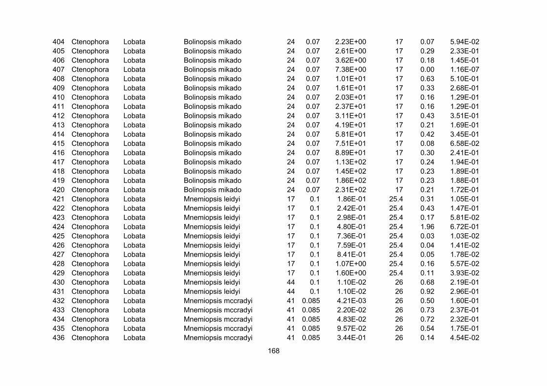
168
404 Ctenophora Lobata Bolinopsis mikado 24 0.07 2.23E+00 17 0.07 5.94E-02405 Ctenophora Lobata Bolinopsis mikado 24 0.07 2.61E+00 17 0.29 2.33E-01406 Ctenophora Lobata Bolinopsis mikado 24 0.07 3.62E+00 17 0.18 1.45E-01407 Ctenophora Lobata Bolinopsis mikado 24 0.07 7.38E+00 17 0.00 1.16E-07408 Ctenophora Lobata Bolinopsis mikado 24 0.07 1.01E+01 17 0.63 5.10E-01409 Ctenophora Lobata Bolinopsis mikado 24 0.07 1.61E+01 17 0.33 2.68E-01410 Ctenophora Lobata Bolinopsis mikado 24 0.07 2.03E+01 17 0.16 1.29E-01411 Ctenophora Lobata Bolinopsis mikado 24 0.07 2.37E+01 17 0.16 1.29E-01412 Ctenophora Lobata Bolinopsis mikado 24 0.07 3.11E+01 17 0.43 3.51E-01413 Ctenophora Lobata Bolinopsis mikado 24 0.07 4.19E+01 17 0.21 1.69E-01414 Ctenophora Lobata Bolinopsis mikado 24 0.07 5.81E+01 17 0.42 3.45E-01415 Ctenophora Lobata Bolinopsis mikado 24 0.07 7.51E+01 17 0.08 6.58E-02416 Ctenophora Lobata Bolinopsis mikado 24 0.07 8.89E+01 17 0.30 2.41E-01417 Ctenophora Lobata Bolinopsis mikado 24 0.07 1.13E+02 17 0.24 1.94E-01418 Ctenophora Lobata Bolinopsis mikado 24 0.07 1.45E+02 17 0.23 1.89E-01419 Ctenophora Lobata Bolinopsis mikado 24 0.07 1.86E+02 17 0.23 1.88E-01420 Ctenophora Lobata Bolinopsis mikado 24 0.07 2.31E+02 17 0.21 1.72E-01421 Ctenophora Lobata Mnemiopsis leidyi 17 0.1 1.86E-01 25.4 0.31 1.05E-01422 Ctenophora Lobata Mnemiopsis leidyi 17 0.1 2.42E-01 25.4 0.43 1.47E-01423 Ctenophora Lobata Mnemiopsis leidyi 17 0.1 2.98E-01 25.4 0.17 5.81E-02424 Ctenophora Lobata Mnemiopsis leidyi 17 0.1 4.80E-01 25.4 1.96 6.72E-01425 Ctenophora Lobata Mnemiopsis leidyi 17 0.1 7.36E-01 25.4 0.03 1.03E-02426 Ctenophora Lobata Mnemiopsis leidyi 17 0.1 7.59E-01 25.4 0.04 1.41E-02427 Ctenophora Lobata Mnemiopsis leidyi 17 0.1 8.41E-01 25.4 0.05 1.78E-02428 Ctenophora Lobata Mnemiopsis leidyi 17 0.1 1.07E+00 25.4 0.16 5.57E-02429 Ctenophora Lobata Mnemiopsis leidyi 17 0.1 1.60E+00 25.4 0.11 3.93E-02430 Ctenophora Lobata Mnemiopsis leidyi 44 0.1 1.10E-02 26 0.68 2.19E-01431 Ctenophora Lobata Mnemiopsis leidyi 44 0.1 1.10E-02 26 0.92 2.96E-01432 Ctenophora Lobata Mnemiopsis mccradyi 41 0.085 4.21E-03 26 0.50 1.60E-01433 Ctenophora Lobata Mnemiopsis mccradyi 41 0.085 2.20E-02 26 0.73 2.37E-01434 Ctenophora Lobata Mnemiopsis mccradyi 41 0.085 4.83E-02 26 0.72 2.32E-01435 Ctenophora Lobata Mnemiopsis mccradyi 41 0.085 9.57E-02 26 0.54 1.75E-01436 Ctenophora Lobata Mnemiopsis mccradyi 41 0.085 3.44E-01 26 0.14 4.54E-02
169
437 Ctenophora Lobata Mnemiopsis mccradyi 41 0.085 8.38E-01 26 0.33 1.06E-01438 Ctenophora Lobata Mnemiopsis mccradyi 41 0.085 1.28E+00 26 0.48 1.53E-01439 Ctenophora Lobata Mnemiopsis mccradyi 41 0.085 1.54E+00 26 0.24 7.59E-02440 Ctenophora Lobata Mnemiopsis mccradyi 41 0.085 2.51E+00 26 0.11 3.55E-02441 Ctenophora Lobata Mnemiopsis mccradyi 41 0.085 3.21E+00 26 0.06 1.88E-02442 Ctenophora Lobata Mnemiopsis mccradyi 41 0.085 4.98E+00 26 0.37 1.21E-01443 Ctenophora Lobata Mnemiopsis mccradyi 41 0.085 6.96E+00 26 0.09 2.94E-02444 Ctenophora Lobata Mnemiopsis mccradyi 41 0.085 8.13E+00 26 0.04 1.45E-02445 Ctenophora Lobata Mnemiopsis mccradyi 41 0.085 9.61E+00 26 0.09 3.02E-02446 Ctenophora Lobata Mnemiopsis mccradyi 41 0.085 9.74E+00 26 0.16 5.30E-02447 Ctenophora Lobata Mnemiopsis mccradyi 41 0.085 1.26E+01 26 0.08 2.58E-02448 Ctenophora Lobata Mnemiopsis mccradyi 41 0.085 1.91E+01 26 0.09 2.87E-02449 Ctenophora Lobata Mnemiopsis mccradyi 41 0.085 7.52E-03 31 0.66 1.27E-01450 Ctenophora Lobata Mnemiopsis mccradyi 41 0.085 3.59E-02 31 0.44 8.38E-02451 Ctenophora Lobata Mnemiopsis mccradyi 41 0.085 5.49E-02 31 1.35 2.60E-01452 Ctenophora Lobata Mnemiopsis mccradyi 41 0.085 1.63E-01 31 0.49 9.46E-02453 Ctenophora Lobata Mnemiopsis mccradyi 41 0.085 4.81E-01 31 0.24 4.54E-02454 Ctenophora Lobata Mnemiopsis mccradyi 41 0.085 8.82E-01 31 0.23 4.36E-02455 Ctenophora Lobata Mnemiopsis mccradyi 41 0.085 1.39E+00 31 0.24 4.54E-02456 Ctenophora Lobata Mnemiopsis mccradyi 41 0.085 1.87E+00 31 0.31 5.91E-02457 Ctenophora Lobata Mnemiopsis mccradyi 41 0.085 2.93E+00 31 0.20 3.83E-02458 Ctenophora Lobata Mnemiopsis mccradyi 41 0.085 1.52E-03 21 0.33 1.78E-01459 Ctenophora Lobata Mnemiopsis mccradyi 41 0.085 3.89E-03 21 1.45 7.83E-01460 Ctenophora Lobata Mnemiopsis mccradyi 41 0.085 9.87E-03 21 0.38 2.08E-01461 Ctenophora Lobata Mnemiopsis mccradyi 41 0.085 1.76E-02 21 0.38 2.04E-01462 Ctenophora Lobata Mnemiopsis mccradyi 41 0.085 2.99E-02 21 1.09 5.90E-01463 Ctenophora Lobata Mnemiopsis mccradyi 41 0.085 4.53E-02 21 0.93 4.99E-01464 Ctenophora Lobata Mnemiopsis mccradyi 41 0.085 7.69E-02 21 0.21 1.14E-01465 Ctenophora Lobata Mnemiopsis mccradyi 41 0.085 2.94E-01 21 0.35 1.91E-01466 Ctenophora Lobata Mnemiopsis mccradyi 41 0.085 3.67E-01 21 0.15 7.91E-02467 Ctenophora Lobata Mnemiopsis mccradyi 41 0.085 4.06E-01 21 0.07 3.79E-02468 Ctenophora Lobata Mnemiopsis mccradyi 41 0.085 6.14E-01 21 0.24 1.32E-01469 Ctenophora Lobata Mnemiopsis mccradyi 41 0.085 1.19E+00 21 0.29 1.56E-01
170
470 Ctenophora Lobata Mnemiopsis mccradyi 41 0.085 1.73E+00 21 0.10 5.53E-02471 Ctenophora Lobata Mnemiopsis mccradyi 41 0.085 2.07E+00 21 0.21 1.11E-01472 Ctenophora Lobata Mnemiopsis mccradyi 41 0.085 2.64E+00 21 0.48 2.56E-01473 Ctenophora Lobata Mnemiopsis mccradyi 41 0.085 3.38E+00 21 0.07 3.68E-02474 Ctenophora Lobata Mnemiopsis mccradyi 41 0.085 4.55E+00 21 0.24 1.27E-01475 Ctenophora Lobata Mnemiopsis mccradyi 41 0.085 6.87E+00 21 0.07 3.74E-02476 Ctenophora Lobata Mnemiopsis mccradyi 41 0.085 9.74E+00 21 0.14 7.73E-02477 Ctenophora Lobata Mnemiopsis mccradyi 41 0.085 1.21E+01 21 0.06 3.44E-02478 Ctenophora Lobata Mnemiopsis mccradyi 30 0.085 1.57E-01 26 0.78 2.52E-01479 Ctenophora Lobata Mnemiopsis mccradyi 30 0.085 3.27E-01 26 0.64 2.08E-01480 Ctenophora Lobata Mnemiopsis mccradyi 30 0.085 5.99E-01 26 0.40 1.29E-01481 Ctenophora Lobata Mnemiopsis mccradyi 30 0.085 4.13E-01 26 0.38 1.24E-01482 Ctenophora Lobata Mnemiopsis mccradyi 30 0.085 2.56E+00 26 0.53 1.69E-01483 Ctenophora Lobata Mnemiopsis mccradyi 30 0.085 1.82E+00 26 0.34 1.08E-01484 Ctenophora Lobata Mnemiopsis mccradyi 30 0.085 3.69E+00 21 0.24 1.29E-01485 Ctenophora Nuda Beroe ovata 26 0.16 8.16E+01 26 0.21 6.68E-02486 Ctenophora Nuda Beroe ovata 26 0.16 9.05E+01 26 0.00 2.64E-08487 Ctenophora Nuda Beroe ovata 26 0.16 9.65E+01 26 0.13 4.11E-02488 Ctenophora Nuda Beroe ovata 26 0.16 1.13E+02 26 0.18 5.87E-02489 Ctenophora Nuda Beroe ovata 26 0.16 1.31E+02 26 0.12 3.79E-02490 Ctenophora Nuda Beroe ovata 26 0.16 1.47E+02 26 0.11 3.61E-02491 Ctenophora Nuda Beroe ovata 26 0.16 1.64E+02 26 0.11 3.44E-02492 Ctenophora Nuda Beroe ovata 26 0.16 1.77E+02 26 0.05 1.59E-02493 Ctenophora Nuda Beroe ovata 26 0.16 1.82E+02 26 0.00 9.11E-04494 Ctenophora Nuda Beroe ovata 26 0.16 1.91E+02 26 0.10 3.12E-02495 Ctenophora Nuda Beroe ovata 26 0.16 5.25E+01 26 0.19 5.98E-02496 Ctenophora Nuda Beroe ovata 26 0.16 5.50E+01 26 0.09 3.01E-02497 Ctenophora Nuda Beroe ovata 26 0.16 6.97E+01 26 0.38 1.23E-01498 Ctenophora Nuda Beroe ovata 26 0.16 1.02E+02 26 0.38 1.21E-01499 Ctenophora Nuda Beroe ovata 26 0.16 1.27E+02 26 0.06 1.96E-02500 Ctenophora Nuda Beroe ovata 26 0.16 1.34E+02 26 0.06 1.85E-02501 Ctenophora Nuda Beroe ovata 26 0.16 1.38E+02 26 0.00 1.64E-09502 Ctenophora Nuda Beroe ovata 26 0.16 5.35E+01 26 0.00 7.48E-08

171
503 Ctenophora Nuda Beroe ovata 26 0.16 5.35E+01 26 0.00 6.73E-08504 Ctenophora Nuda Beroe ovata 26 0.16 5.82E+01 26 0.17 5.40E-02505 Ctenophora Nuda Beroe ovata 26 0.16 5.60E+01 26 0.09 2.95E-02506 Ctenophora Nuda Beroe ovata 26 0.16 6.57E+01 26 0.23 7.29E-02507 Ctenophora Nuda Beroe ovata 26 0.16 7.88E+01 26 0.14 4.41E-02508 Ctenophora Nuda Beroe ovata 26 0.16 8.43E+01 26 0.00 1.61E-08509 Ctenophora Nuda Beroe ovata 26 0.16 8.71E+01 26 0.06 2.09E-02510 Ctenophora Nuda Beroe ovata 26 0.16 9.30E+01 26 0.07 2.13E-02511 Ctenophora Nuda Beroe ovata 26 0.16 9.97E+01 26 0.07 2.32E-02512 Chordata Salpida Thalia democratica 11 0.87 6.29E-03 20 0.34 2.01E-01513 Chordata Salpida Thalia democratica 11 0.87 8.04E-03 20 0.16 9.28E-02514 Chordata Salpida Thalia democratica 11 0.87 1.01E-02 20 0.31 1.86E-01515 Chordata Salpida Thalia democratica 11 0.87 1.32E-02 20 0.22 1.31E-01516 Chordata Salpida Thalia democratica 11 0.87 1.53E-02 20 0.06 3.86E-02517 Chordata Salpida Thalia democratica 11 0.87 1.60E-02 20 0.03 1.54E-02518 Chordata Salpida Thalia democratica 11 0.87 3.53E-03 20 0.04 2.31E-02519 Chordata Salpida Thalia democratica 11 0.87 3.68E-03 20 0.04 2.57E-02520 Chordata Salpida Thalia democratica 11 0.87 4.15E-03 20 0.20 1.19E-01521 Chordata Salpida Thalia democratica 11 0.87 5.02E-03 20 0.18 1.08E-01522 Chordata Salpida Thalia democratica 11 0.87 5.86E-03 20 0.13 7.73E-02523 Chordata Salpida Thalia democratica 11 0.87 6.73E-03 20 0.15 8.76E-02524 Cnidaria Scyphomedusae Aurelia aurita 36 0.2 1.99E-02 15 0.25 2.51E-01525 Cnidaria Scyphomedusae Aurelia aurita 3 0.2 1.24E-03 6 0.24 5.98E-01526 Cnidaria Scyphomedusae Aurelia aurita 3 0.2 1.99E-03 9.5 0.20 3.58E-01527 Cnidaria Scyphomedusae Aurelia aurita 3 0.2 3.03E-03 12 0.32 4.32E-01528 Cnidaria Scyphomedusae Aurelia aurita 3 0.2 1.77E-03 15 0.25 2.48E-01529 Cnidaria Scyphomedusae Aurelia aurita 3 0.2 4.79E-03 18 0.39 2.88E-01530 Cnidaria Scyphomedusae Aurelia aurita 3 0.2 1.48E-03 15 0.25 2.54E-01531 Cnidaria Scyphomedusae Aurelia aurita 3 0.2 4.65E-03 18 0.41 2.97E-01532 Cnidaria Scyphomedusae Aurelia aurita 14 0.2 3.82E-02 15 0.24 2.38E-01533 Cnidaria Scyphomedusae Aurelia aurita 14 0.2 3.84E-02 15 0.21 2.08E-01534 Cnidaria Scyphomedusae Aurelia labiata 51 0.2 9.78E-03 10 0.07 1.12E-01535 Cnidaria Scyphomedusae Aurelia labiata 51 0.2 1.22E-02 12 0.10 1.35E-01
172
536 Cnidaria Scyphomedusae Aurelia labiata 51 0.2 2.07E-02 15 0.17 1.74E-01537 Cnidaria Scyphomedusae Aurelia labiata 51 0.2 2.48E-02 17 0.20 1.63E-01538 Cnidaria Scyphomedusae Aurelia labiata 51 0.2 3.29E-02 21 0.24 1.30E-01539 Cnidaria Scyphomedusae Aurelia labiata 51 0.2 2.66E-02 22.5 0.21 9.69E-02540 Cnidaria Scyphomedusae Aurelia labiata 51 0.2 2.07E-02 24.5 0.17 6.53E-02541 Cnidaria Scyphomedusae Aurelia labiata 51 0.2 1.08E-02 26 0.08 2.63E-02542 Cnidaria Scyphomedusae Aurelia labiata 51 0.2 1.17E-02 28 0.09 2.42E-02543 Cnidaria Scyphomedusae Chrysaora quinquecirrha 37 0.53 9.32E-03 23 0.74 3.25E-01544 Cnidaria Scyphomedusae Chrysaora quinquecirrha 31 0.53 2.39E+00 27.5 0.09 2.57E-02545 Cnidaria Scyphomedusae Chrysaora quinquecirrha 31 0.53 6.39E+00 27.5 0.04 1.06E-02546 Cnidaria Scyphomedusae Chrysaora quinquecirrha 31 0.53 1.06E+01 27.5 0.05 1.41E-02547 Cnidaria Scyphomedusae Chrysaora quinquecirrha 31 0.53 1.50E+01 27.5 0.01 2.78E-03548 Cnidaria Scyphomedusae Chrysaora quinquecirrha 31 0.53 1.72E+01 27.5 0.01 2.92E-03549 Cnidaria Scyphomedusae Chrysaora quinquecirrha 31 0.53 1.93E+01 27.5 0.00 1.31E-03550 Cnidaria Scyphomedusae Chrysaora quinquecirrha 31 0.53 2.02E+01 27.5 0.00 8.51E-04551 Cnidaria Scyphomedusae Nemopilema nomurai 25 0.55 1.08E+01 25 0.07 2.63E-02552 Cnidaria Scyphomedusae Nemopilema nomurai 25 0.55 2.17E+01 25 0.05 1.87E-02553 Cnidaria Scyphomedusae Nemopilema nomurai 25 0.55 4.74E+01 25 0.09 3.21E-02554 Cnidaria Scyphomedusae Nemopilema nomurai 25 0.55 1.10E+02 25 0.06 2.25E-02555 Cnidaria Scyphomedusae Pelagia noctiluca 32 0.35 1.95E-01 27.5 0.08 2.34E-02556 Cnidaria Scyphomedusae Pelagia noctiluca 32 0.35 2.80E-01 27.5 0.02 5.32E-03557 Cnidaria Scyphomedusae Pelagia noctiluca 32 0.35 1.85E-01 27.5 0.09 2.41E-02558 Cnidaria Scyphomedusae Pelagia noctiluca 32 0.35 1.33E-01 27.5 0.10 2.82E-02559 Cnidaria Scyphomedusae Pelagia noctiluca 32 0.35 2.21E-01 27.5 0.04 1.19E-02560 Cnidaria Scyphomedusae Pelagia noctiluca 32 0.35 1.40E-01 27.5 0.06 1.60E-02
Record Mass g (d-1) Food offered1 2.38E-02 Fed so that no more than 50% of copepod prey were removed2 3.50E-02 Fed so that no more than 50% of copepod prey were removed3 4.57E-02 Fed so that no more than 50% of copepod prey were removed4 5.70E-02 Fed so that no more than 50% of copepod prey were removed5 6.65E-02 Fed so that no more than 50% of copepod prey were removed
173
6 7.54E-02 Fed so that no more than 50% of copepod prey were removed7 2.82E-02 Fed so that no more than 50% of copepod prey were removed8 1.66E-02 Fed so that no more than 50% of copepod prey were removed9 2.00E-02 Fed so that no more than 50% of copepod prey were removed10 2.93E-02 Fed so that no more than 50% of copepod prey were removed11 3.83E-02 Fed so that no more than 50% of copepod prey were removed12 4.77E-02 Fed so that no more than 50% of copepod prey were removed13 5.56E-02 Fed so that no more than 50% of copepod prey were removed14 6.31E-02 Fed so that no more than 50% of copepod prey were removed15 1.50E-02 Fed so that no more than 50% of copepod prey were removed16 1.58E-03 Fed so that no more than 50% of copepod prey were removed17 1.40E-02 Fed so that no more than 50% of copepod prey were removed18 2.05E-02 Fed so that no more than 50% of copepod prey were removed19 2.68E-02 Fed so that no more than 50% of copepod prey were removed20 3.34E-02 Fed so that no more than 50% of copepod prey were removed21 3.90E-02 Fed so that no more than 50% of copepod prey were removed22 1.18E-02 Fed so that no more than 50% of copepod prey were removed23 4.97E-03 Fed so that no more than 50% of copepod prey were removed24 2.91E-02 Recently hatched Artemia added daily25 2.24E-02 Recently hatched Artemia added daily26 3.19E-02 Recently hatched Artemia added daily27 2.85E-04 Recently hatched Artemia added daily28 1.63E-02 Recently hatched Artemia added daily29 2.66E-02 Laboratory high food (see Hirst & Bunker 2002)30 5.65E-02 Laboratory high food (see Hirst & Bunker 2002)31 4.41E-02 Laboratory high food (see Hirst & Bunker 2002)32 2.80E-02 Laboratory high food (see Hirst & Bunker 2002)33 2.97E-02 Laboratory high food (see Hirst & Bunker 2002)34 2.64E-02 Laboratory high food (see Hirst & Bunker 2002)35 4.26E-02 Laboratory high food (see Hirst & Bunker 2002)36 2.92E-02 Laboratory high food (see Hirst & Bunker 2002)37 7.60E-02 Laboratory high food (see Hirst & Bunker 2002)38 1.63E-01 Laboratory high food (see Hirst & Bunker 2002)

174
39 3.90E-02 Laboratory high food (see Hirst & Bunker 2002)40 9.00E-02 Laboratory high food (see Hirst & Bunker 2002)41 6.59E-02 Laboratory high food (see Hirst & Bunker 2002)42 9.17E-02 Laboratory high food (see Hirst & Bunker 2002)43 1.15E-01 Laboratory high food (see Hirst & Bunker 2002)44 6.89E-02 Laboratory high food (see Hirst & Bunker 2002)45 8.52E-02 Laboratory high food (see Hirst & Bunker 2002)46 1.18E-02 Laboratory high food (see Hirst & Bunker 2002)47 8.81E-02 Laboratory high food (see Hirst & Bunker 2002)48 2.26E-02 Laboratory high food (see Hirst & Bunker 2002)49 9.60E-02 Laboratory high food (see Hirst & Bunker 2002)50 1.03E-01 Laboratory high food (see Hirst & Bunker 2002)51 1.04E-01 Laboratory high food (see Hirst & Bunker 2002)52 6.86E-02 Laboratory high food (see Hirst & Bunker 2002)53 1.11E-01 Laboratory high food (see Hirst & Bunker 2002)54 1.22E-01 Laboratory high food (see Hirst & Bunker 2002)55 1.18E-01 Laboratory high food (see Hirst & Bunker 2002)56 8.67E-02 Laboratory high food (see Hirst & Bunker 2002)57 9.46E-02 Laboratory high food (see Hirst & Bunker 2002)58 1.08E-01 Laboratory high food (see Hirst & Bunker 2002)59 1.33E-01 Laboratory high food (see Hirst & Bunker 2002)60 1.18E-01 Laboratory high food (see Hirst & Bunker 2002)61 5.10E-02 Laboratory high food (see Hirst & Bunker 2002)62 5.47E-02 Laboratory high food (see Hirst & Bunker 2002)63 5.53E-02 Laboratory high food (see Hirst & Bunker 2002)64 5.41E-02 Laboratory high food (see Hirst & Bunker 2002)65 5.11E-02 Laboratory high food (see Hirst & Bunker 2002)66 1.86E-01 Laboratory high food (see Hirst & Bunker 2002)67 1.91E-01 Laboratory high food (see Hirst & Bunker 2002)68 1.88E-01 Laboratory high food (see Hirst & Bunker 2002)69 1.79E-01 Laboratory high food (see Hirst & Bunker 2002)70 1.64E-01 Laboratory high food (see Hirst & Bunker 2002)71 1.49E-01 Laboratory high food (see Hirst & Bunker 2002)
175
72 1.40E-01 Laboratory high food (see Hirst & Bunker 2002)73 1.30E-01 Laboratory high food (see Hirst & Bunker 2002)74 1.17E-01 Laboratory high food (see Hirst & Bunker 2002)75 1.01E-01 Laboratory high food (see Hirst & Bunker 2002)76 5.87E-02 Laboratory high food (see Hirst & Bunker 2002)77 5.88E-02 Laboratory high food (see Hirst & Bunker 2002)78 5.70E-02 Laboratory high food (see Hirst & Bunker 2002)79 5.34E-02 Laboratory high food (see Hirst & Bunker 2002)80 4.85E-02 Laboratory high food (see Hirst & Bunker 2002)81 2.49E-02 Laboratory high food (see Hirst & Bunker 2002)82 4.65E-02 Laboratory high food (see Hirst & Bunker 2002)83 3.26E-02 Laboratory high food (see Hirst & Bunker 2002)84 7.13E-02 Laboratory high food (see Hirst & Bunker 2002)85 3.25E-02 Laboratory high food (see Hirst & Bunker 2002)86 6.18E-02 Laboratory high food (see Hirst & Bunker 2002)87 2.18E-02 Laboratory high food (see Hirst & Bunker 2002)88 2.98E-02 Laboratory high food (see Hirst & Bunker 2002)89 3.45E-02 Laboratory high food (see Hirst & Bunker 2002)90 2.18E-02 Laboratory high food (see Hirst & Bunker 2002)91 1.66E-02 Laboratory high food (see Hirst & Bunker 2002)92 6.35E-02 Laboratory high food (see Hirst & Bunker 2002)93 4.41E-02 Laboratory high food (see Hirst & Bunker 2002)94 5.12E-02 Laboratory high food (see Hirst & Bunker 2002)95 1.60E-02 Laboratory high food (see Hirst & Bunker 2002)96 3.52E-02 Laboratory high food (see Hirst & Bunker 2002)97 3.86E-02 Laboratory high food (see Hirst & Bunker 2002)98 4.61E-02 Laboratory high food (see Hirst & Bunker 2002)99 3.32E-02 Laboratory high food (see Hirst & Bunker 2002)100 1.44E-02 Laboratory high food (see Hirst & Bunker 2002)101 3.55E-02 Laboratory high food (see Hirst & Bunker 2002)102 3.61E-02 Laboratory high food (see Hirst & Bunker 2002)103 4.30E-02 Laboratory high food (see Hirst & Bunker 2002)104 3.22E-02 Laboratory high food (see Hirst & Bunker 2002)
176
105 1.36E-02 Laboratory high food (see Hirst & Bunker 2002)106 2.86E-02 Laboratory high food (see Hirst & Bunker 2002)107 3.05E-02 Laboratory high food (see Hirst & Bunker 2002)108 3.93E-02 Laboratory high food (see Hirst & Bunker 2002)109 2.56E-02 Laboratory high food (see Hirst & Bunker 2002)110 1.12E-02 Laboratory high food (see Hirst & Bunker 2002)111 2.21E-02 Laboratory high food (see Hirst & Bunker 2002)112 1.45E-02 Laboratory high food (see Hirst & Bunker 2002)113 3.39E-02 Laboratory high food (see Hirst & Bunker 2002)114 1.05E-02 Laboratory high food (see Hirst & Bunker 2002)115 1.94E-02 Laboratory high food (see Hirst & Bunker 2002)116 1.11E-02 Laboratory high food (see Hirst & Bunker 2002)117 1.89E-02 Laboratory high food (see Hirst & Bunker 2002)118 1.54E-02 Laboratory high food (see Hirst & Bunker 2002)119 1.55E-02 Laboratory high food (see Hirst & Bunker 2002)120 1.52E-02 Laboratory high food (see Hirst & Bunker 2002)121 1.43E-02 Laboratory high food (see Hirst & Bunker 2002)122 1.32E-02 Laboratory high food (see Hirst & Bunker 2002)123 6.15E-02 Laboratory high food (see Hirst & Bunker 2002)124 6.27E-02 Laboratory high food (see Hirst & Bunker 2002)125 6.15E-02 Laboratory high food (see Hirst & Bunker 2002)126 5.86E-02 Laboratory high food (see Hirst & Bunker 2002)127 5.43E-02 Laboratory high food (see Hirst & Bunker 2002)128 2.77E-02 Laboratory high food (see Hirst & Bunker 2002)129 7.28E-02 Laboratory high food (see Hirst & Bunker 2002)130 6.18E-02 Laboratory high food (see Hirst & Bunker 2002)131 3.74E-02 Laboratory high food (see Hirst & Bunker 2002)132 4.35E-02 Laboratory high food (see Hirst & Bunker 2002)133 4.58E-02 Laboratory high food (see Hirst & Bunker 2002)134 4.40E-02 Laboratory high food (see Hirst & Bunker 2002)135 4.80E-02 Laboratory high food (see Hirst & Bunker 2002)136 5.46E-02 Laboratory high food (see Hirst & Bunker 2002)137 5.96E-02 Laboratory high food (see Hirst & Bunker 2002)
177
138 6.22E-02 Laboratory high food (see Hirst & Bunker 2002)139 5.00E-02 Laboratory high food (see Hirst & Bunker 2002)140 5.93E-02 Laboratory high food (see Hirst & Bunker 2002)141 6.63E-02 Laboratory high food (see Hirst & Bunker 2002)142 6.94E-02 Laboratory high food (see Hirst & Bunker 2002)143 6.87E-02 Laboratory high food (see Hirst & Bunker 2002)144 1.97E-02 Laboratory high food (see Hirst & Bunker 2002)145 4.20E-02 Laboratory high food (see Hirst & Bunker 2002)146 1.49E-02 Laboratory high food (see Hirst & Bunker 2002)147 4.06E-02 Laboratory high food (see Hirst & Bunker 2002)148 2.46E-02 Laboratory high food (see Hirst & Bunker 2002)149 3.07E-02 Laboratory high food (see Hirst & Bunker 2002)150 3.35E-02 Laboratory high food (see Hirst & Bunker 2002)151 3.12E-02 Laboratory high food (see Hirst & Bunker 2002)152 2.95E-02 Laboratory high food (see Hirst & Bunker 2002)153 2.33E-02 Laboratory high food (see Hirst & Bunker 2002)154 4.40E-02 Laboratory high food (see Hirst & Bunker 2002)155 6.11E-02 Laboratory high food (see Hirst & Bunker 2002)156 7.40E-02 Laboratory high food (see Hirst & Bunker 2002)157 7.46E-02 Laboratory high food (see Hirst & Bunker 2002)158 7.24E-02 Laboratory high food (see Hirst & Bunker 2002)159 6.14E-02 Laboratory high food (see Hirst & Bunker 2002)160 2.97E-02 Laboratory high food (see Hirst & Bunker 2002)161 6.84E-02 Laboratory high food (see Hirst & Bunker 2002)162 2.90E-02 Laboratory high food (see Hirst & Bunker 2002)163 9.06E-02 Laboratory high food (see Hirst & Bunker 2002)164 1.20E-01 Laboratory high food (see Hirst & Bunker 2002)165 9.43E-02 Fed Coscinodiscus until 200-300ugC in size, then fed Calanus, this reflects natural shift in diet166 1.07E-01 Fed Coscinodiscus until 200-300ugC in size, then fed Calanus, this reflects natural shift in diet167 1.16E-01 Fed Coscinodiscus until 200-300ugC in size, then fed Calanus, this reflects natural shift in diet168 1.28E-01 Fed Coscinodiscus until 200-300ugC in size, then fed Calanus, this reflects natural shift in diet169 1.34E-01 Fed Coscinodiscus until 200-300ugC in size, then fed Calanus, this reflects natural shift in diet170 1.39E-01 Fed Coscinodiscus until 200-300ugC in size, then fed Calanus, this reflects natural shift in diet
178
171 1.45E-01 Fed Coscinodiscus until 200-300ugC in size, then fed Calanus, this reflects natural shift in diet172 1.47E-01 Fed Coscinodiscus until 200-300ugC in size, then fed Calanus, this reflects natural shift in diet173 1.43E-01 Fed Coscinodiscus until 200-300ugC in size, then fed Calanus, this reflects natural shift in diet174 1.38E-01 Fed Coscinodiscus until 200-300ugC in size, then fed Calanus, this reflects natural shift in diet175 9.20E-02 Fed Coscinodiscus until 200-300ugC in size, then fed Calanus, this reflects natural shift in diet176 1.02E-01 Fed Coscinodiscus until 200-300ugC in size, then fed Calanus, this reflects natural shift in diet177 1.10E-01 Fed Coscinodiscus until 200-300ugC in size, then fed Calanus, this reflects natural shift in diet178 1.18E-01 Fed Coscinodiscus until 200-300ugC in size, then fed Calanus, this reflects natural shift in diet179 1.23E-01 Fed Coscinodiscus until 200-300ugC in size, then fed Calanus, this reflects natural shift in diet180 1.25E-01 Fed Coscinodiscus until 200-300ugC in size, then fed Calanus, this reflects natural shift in diet181 1.26E-01 Fed Coscinodiscus until 200-300ugC in size, then fed Calanus, this reflects natural shift in diet182 1.24E-01 Fed Coscinodiscus until 200-300ugC in size, then fed Calanus, this reflects natural shift in diet183 1.17E-01 Fed Coscinodiscus until 200-300ugC in size, then fed Calanus, this reflects natural shift in diet184 1.08E-01 Fed Coscinodiscus until 200-300ugC in size, then fed Calanus, this reflects natural shift in diet185 8.64E-02 Fed Coscinodiscus until 200-300ugC in size, then fed Calanus, this reflects natural shift in diet186 9.61E-02 Fed Coscinodiscus until 200-300ugC in size, then fed Calanus, this reflects natural shift in diet187 1.05E-01 Fed Coscinodiscus until 200-300ugC in size, then fed Calanus, this reflects natural shift in diet188 1.16E-01 Fed Coscinodiscus until 200-300ugC in size, then fed Calanus, this reflects natural shift in diet189 1.23E-01 Fed Coscinodiscus until 200-300ugC in size, then fed Calanus, this reflects natural shift in diet190 1.26E-01 Fed Coscinodiscus until 200-300ugC in size, then fed Calanus, this reflects natural shift in diet191 1.29E-01 Fed Coscinodiscus until 200-300ugC in size, then fed Calanus, this reflects natural shift in diet192 1.28E-01 Fed Coscinodiscus until 200-300ugC in size, then fed Calanus, this reflects natural shift in diet193 1.20E-01 Fed Coscinodiscus until 200-300ugC in size, then fed Calanus, this reflects natural shift in diet194 1.09E-01 Fed Coscinodiscus until 200-300ugC in size, then fed Calanus, this reflects natural shift in diet195 4.68E-02 Maintained on excess food196 7.53E-02 Maintained on excess food197 3.53E-02 Maintained on excess food198 2.93E-02 Maintained on excess food199 2.74E-02 Maintained on excess food200 2.48E-02 Maintained on excess food201 2.60E-02 Maintained on excess food202 6.26E-02 Maintained on excess food203 3.84E-02 Maintained on excess food
179
204 3.23E-02 Maintained on excess food205 3.00E-02 Maintained on excess food206 2.74E-02 Maintained on excess food207 2.37E-02 Supplied with a surplus of Artemia nauplii as food.208 2.25E-02 Supplied with a surplus of Artemia nauplii as food.209 2.08E-02 Supplied with a surplus of Artemia nauplii as food.210 1.26E-02 Supplied with a surplus of Artemia nauplii as food.211 1.09E-02 Supplied with a surplus of Artemia nauplii as food.212 7.53E-03 Supplied with a surplus of Artemia nauplii as food.213 1.14E-02 Supplied with a surplus of Artemia nauplii as food.214 6.20E-03 Supplied with a surplus of Artemia nauplii as food.215 4.67E-03 Supplied with a surplus of Artemia nauplii as food.216 7.28E-02 Phaeodactylum tricornutum fed once weekly 10^5 cells/ml217 6.48E-02 Phaeodactylum tricornutum fed once weekly 10^5 cells/ml218 6.81E-02 Phaeodactylum tricornutum fed once weekly 10^5 cells/ml219 5.20E-02 Phaeodactylum tricornutum fed once weekly 10^5 cells/ml220 5.37E-02 Phaeodactylum tricornutum fed once weekly 10^5 cells/ml221 4.12E-02 Phaeodactylum tricornutum fed once weekly 10^5 cells/ml222 4.53E-02 Phaeodactylum tricornutum fed once weekly 10^5 cells/ml223 3.95E-02 Phaeodactylum tricornutum fed once weekly 10^5 cells/ml224 3.32E-02 Phaeodactylum tricornutum fed once weekly 10^5 cells/ml225 2.42E-02 Phaeodactylum tricornutum fed once weekly 10^5 cells/ml226 5.33E-02 Laboratory high food227 7.30E-02 Laboratory high food228 5.12E-02 Laboratory high food229 7.75E-02 Laboratory high food230 4.76E-02 Laboratory high food231 5.90E-02 Laboratory high food232 3.31E-02 Laboratory high food233 1.83E-02 Laboratory high food234 6.66E-02 Laboratory high food235 6.16E-02 Laboratory high food236 4.65E-02 Laboratory high food
180
237 5.39E-02 Laboratory high food238 1.49E-02 Laboratory high food239 1.11E-01 Laboratory high food240 5.06E-02 Laboratory high food241 4.84E-02 Laboratory high food242 4.99E-02 Laboratory high food243 1.57E-02 Laboratory high food244 2.77E-02 Laboratory high food245 8.37E-02 Laboratory high food246 7.35E-02 Laboratory high food247 5.00E-02 Laboratory high food248 4.72E-02 Laboratory high food249 2.76E-02 Laboratory high food250 1.01E-02 Laboratory high food251 5.52E-02 Laboratory high food252 9.07E-02 Laboratory high food253 3.51E-02 Laboratory high food254 4.20E-02 Laboratory high food255 2.53E-02 Laboratory high food256 9.49E-02 Laboratory high food257 2.70E-02 Laboratory high food258 1.32E-02 Laboratory high food259 5.69E-03 Laboratory high food260 2.98E-03 Laboratory high food261 2.46E-03 Laboratory high food262 1.25E-03 Laboratory high food263 6.32E-04 Laboratory high food264 2.35E-02 Laboratory high food265 1.16E-02 Laboratory high food266 5.35E-03 Laboratory high food267 2.80E-03 Laboratory high food268 1.72E-03 Laboratory high food269 5.82E-04 Laboratory high food
181
270 5.86E-04 Laboratory high food271 6.85E-02 Artemia nauplii with supplementary frozen zoop to excess272 6.29E-02 Artemia nauplii with supplementary frozen zoop to excess273 5.89E-02 Artemia nauplii with supplementary frozen zoop to excess274 5.50E-02 Artemia nauplii with supplementary frozen zoop to excess275 5.18E-02 Artemia nauplii with supplementary frozen zoop to excess276 4.86E-02 Artemia nauplii with supplementary frozen zoop to excess277 4.60E-02 Artemia nauplii with supplementary frozen zoop to excess278 4.30E-02 Artemia nauplii with supplementary frozen zoop to excess279 4.05E-02 Artemia nauplii with supplementary frozen zoop to excess280 3.80E-02 Artemia nauplii with supplementary frozen zoop to excess281 3.53E-02 Artemia nauplii with supplementary frozen zoop to excess282 7.86E-02 Artemia nauplii with supplementary frozen zoop to excess283 7.23E-02 Artemia nauplii with supplementary frozen zoop to excess284 6.76E-02 Artemia nauplii with supplementary frozen zoop to excess285 6.31E-02 Artemia nauplii with supplementary frozen zoop to excess286 5.94E-02 Artemia nauplii with supplementary frozen zoop to excess287 5.58E-02 Artemia nauplii with supplementary frozen zoop to excess288 5.70E-02 Artemia nauplii with supplementary frozen zoop to excess289 4.95E-02 Artemia nauplii with supplementary frozen zoop to excess290 4.65E-02 Artemia nauplii with supplementary frozen zoop to excess291 4.35E-02 Artemia nauplii with supplementary frozen zoop to excess292 4.05E-02 Artemia nauplii with supplementary frozen zoop to excess293 6.60E-02 Artemia nauplii with supplementary frozen zoop to excess294 6.07E-02 Artemia nauplii with supplementary frozen zoop to excess295 5.67E-02 Artemia nauplii with supplementary frozen zoop to excess296 5.30E-02 Artemia nauplii with supplementary frozen zoop to excess297 4.98E-02 Artemia nauplii with supplementary frozen zoop to excess298 4.69E-02 Artemia nauplii with supplementary frozen zoop to excess299 4.42E-02 Artemia nauplii with supplementary frozen zoop to excess300 4.15E-02 Artemia nauplii with supplementary frozen zoop to excess301 3.89E-02 Artemia nauplii with supplementary frozen zoop to excess302 3.65E-02 Artemia nauplii with supplementary frozen zoop to excess
182
303 3.39E-02 Artemia nauplii with supplementary frozen zoop to excess304 6.86E-02 Natural assemblage but concentration unknown305 1.88E-01 Natural assemblage but concentration unknown306 9.71E-02 Natural assemblage but concentration unknown307 3.35E-02 Natural assemblage but concentration unknown308 4.52E-02 Natural assemblage but concentration unknown309 1.48E-02 Natural assemblage but concentration unknown310 4.97E-02 Natural assemblage but concentration unknown311 4.31E-03 Natural assemblage but concentration unknown312 1.03E-03 Natural assemblage but concentration unknown313 3.01E-02 Natural assemblage but concentration unknown314 6.72E-02 Natural assemblage but concentration unknown315 1.36E-01 Natural assemblage but concentration unknown316 1.88E-01 Natural assemblage but concentration unknown317 4.45E-01 Natural assemblage but concentration unknown318 5.08E-02 Natural assemblage but concentration unknown319 6.45E-02 Natural assemblage but concentration unknown320 2.85E-02 Natural assemblage but concentration unknown321 8.35E-02 Natural assemblage but concentration unknown322 2.04E-02 Natural assemblage but concentration unknown323 8.77E-02 Natural assemblage but concentration unknown324 1.43E-01 Natural assemblage but concentration unknown325 1.49E-01 Natural assemblage but concentration unknown326 2.11E-01 Natural assemblage but concentration unknown327 1.05E-01 Natural assemblage but concentration unknown328 6.27E-02 Natural assemblage but concentration unknown329 9.65E-02 Natural assemblage but concentration unknown330 1.58E-02 Natural assemblage but concentration unknown331 1.25E-01 Deep tank, natural assemblage but concentration not givwn332 1.49E-01 Deep tank, natural assemblage but concentration not givwn333 1.10E-01 Deep tank, natural assemblage but concentration not givwn334 4.28E-02 Deep tank, natural assemblage but concentration not givwn335 5.95E-02 Deep tank, natural assemblage but concentration not givwn
183
336 3.23E-02 Deep tank, natural assemblage but concentration not givwn337 5.31E-02 Deep tank, natural assemblage but concentration not givwn338 1.43E-01 Deep tank, natural assemblage but concentration not givwn339 1.35E-01 Deep tank, natural assemblage but concentration not givwn340 7.00E-02 Deep tank, natural assemblage but concentration not givwn341 2.93E-02 Deep tank, natural assemblage but concentration not givwn342 1.93E-02 Rhodomonas and Thalassiosira (no more then 30% removed)343 7.65E-02 Rhodomonas and Thalassiosira (no more then 30% removed)344 1.10E-01 Rhodomonas and Thalassiosira (no more then 30% removed)345 1.11E-01 Rhodomonas and Thalassiosira (no more then 30% removed)346 1.07E-01 Rhodomonas and Thalassiosira (no more then 30% removed)347 8.56E-02 Rhodomonas and Thalassiosira (no more then 30% removed)348 6.19E-02 Rhodomonas and Thalassiosira (no more then 30% removed)349 7.10E-02 Rhodomonas and Thalassiosira (no more then 30% removed)350 4.89E-02 Rhodomonas and Thalassiosira (no more then 30% removed)351 5.60E-02 Rhodomonas and Thalassiosira (no more then 30% removed)352 6.42E-02 Rhodomonas and Thalassiosira (no more then 30% removed)353 6.20E-02 Rhodomonas and Thalassiosira (no more then 30% removed)354 1.32E-02 0.2-0.6 Isochrysis and 0.1-0.3 Peridinium l-13355 1.22E-02 0.2-0.6 Isochrysis and 0.1-0.3 Peridinium l-14356 3.33E-02 0.2-0.6 Isochrysis and 0.1-0.3 Peridinium l-15357 3.95E-02 0.2-0.6 Isochrysis and 0.1-0.3 Peridinium l-16358 2.97E-02 0.2-0.6 Isochrysis and 0.1-0.3 Peridinium l-17359 3.74E-02 0.2-0.6 Isochrysis and 0.1-0.3 Peridinium l-18360 3.77E-02 0.2-0.6 Isochrysis and 0.1-0.3 Peridinium l-19361 4.13E-02 0.2-0.6 Isochrysis and 0.1-0.3 Peridinium l-20362 1.67E-02 0.2-0.6 Isochrysis and 0.1-0.3 Peridinium l-21363 2.37E-02 0.2-0.6 Isochrysis and 0.1-0.3 Peridinium l-22364 1.67E-01 "Mixed diet"" - included gelatinous prey365 1.72E-01 "Mixed diet"" - included gelatinous prey366 2.23E-01 "Mixed diet"" - included gelatinous prey367 1.96E-01 "Mixed diet"" - included gelatinous prey368 1.61E-01 "Mixed diet"" - included gelatinous prey
184
369 1.50E-01 "Mixed diet"" - included gelatinous prey370 6.81E-02 "Mixed diet"" - included gelatinous prey371 3.42E-02 "Mixed diet"" - included gelatinous prey372 1.08E-01373 9.39E-02374 5.28E-02375 5.69E-02376 6.24E-02377 9.04E-02378 6.88E-02 Artemia nauplii in excess379 6.41E-02 Artemia nauplii in excess380 4.22E-02 Artemia nauplii in excess381 4.93E-02 Artemia nauplii in excess382 2.30E-02 Artemia nauplii in excess383 1.83E-01 Fresh copepods to excess384 1.18E-01 Fresh copepods to excess385 1.07E-01 Fresh copepods to excess386 7.44E-02 Fresh copepods to excess387 7.60E-02 Fresh copepods to excess388 7.87E-02 Fresh copepods to excess389 4.72E-02 Fresh copepods to excess390 4.51E-02 Fresh copepods to excess391 9.77E-02 100 Acartia l-1392 9.90E-01 100 Acartia l-1393 1.09E+00 100 Acartia l-1394 5.13E-01 100 Acartia l-1395 2.59E-01 100 Acartia l-1396 1.79E-01 100 Acartia l-1397 4.48E-01 100 Acartia l-1398 4.89E-01 100 Acartia l-1399 1.07E+00 100 Acartia l-1400 2.63E-01 100 Acartia l-1401 2.49E-01 100 Acartia l-1
185
402 1.56E-01 100 Acartia l-1403 5.35E-01 101 Acartia l-1404 7.26E-02 102 Acartia l-1405 2.97E-01 103 Acartia l-1406 2.00E-01 104 Acartia l-1407 1.91E-07 105 Acartia l-1408 9.09E-01 106 Acartia l-1409 5.37E-01 107 Acartia l-1410 2.74E-01 108 Acartia l-1411 2.86E-01 109 Acartia l-1412 8.30E-01 110 Acartia l-1413 4.31E-01 111 Acartia l-1414 9.53E-01 112 Acartia l-1415 1.94E-01 113 Acartia l-1416 7.41E-01 114 Acartia l-1417 6.33E-01 115 Acartia l-1418 6.58E-01 116 Acartia l-1419 6.96E-01 117 Acartia l-1420 6.69E-01 118 Acartia l-1421 6.88E-02422 1.03E-01423 4.29E-02424 5.60E-01425 9.51E-03426 1.31E-02427 1.70E-02428 5.66E-02429 4.42E-02430 7.10E-02431 9.60E-02432 4.07E-02 Acartia/Paracalanus so that conc never dropped below 50%433 9.12E-02 Acartia/Paracalanus so that conc never dropped below 50%434 1.09E-01 Acartia/Paracalanus so that conc never dropped below 50%
186
435 9.73E-02 Acartia/Paracalanus so that conc never dropped below 50%436 3.47E-02 Acartia/Paracalanus so that conc never dropped below 50%437 1.01E-01 Acartia/Paracalanus so that conc never dropped below 50%438 1.63E-01 Acartia/Paracalanus so that conc never dropped below 50%439 8.45E-02 Acartia/Paracalanus so that conc never dropped below 50%440 4.47E-02 Acartia/Paracalanus so that conc never dropped below 50%441 2.52E-02 Acartia/Paracalanus so that conc never dropped below 50%442 1.80E-01 Acartia/Paracalanus so that conc never dropped below 50%443 4.77E-02 Acartia/Paracalanus so that conc never dropped below 50%444 2.45E-02 Acartia/Paracalanus so that conc never dropped below 50%445 5.32E-02 Acartia/Paracalanus so that conc never dropped below 50%446 9.36E-02 Acartia/Paracalanus so that conc never dropped below 50%447 4.86E-02 Acartia/Paracalanus so that conc never dropped below 50%448 5.99E-02 Acartia/Paracalanus so that conc never dropped below 50%449 3.73E-02 Acartia/Paracalanus so that conc never dropped below 50%450 3.65E-02 Acartia/Paracalanus so that conc never dropped below 50%451 1.26E-01 Acartia/Paracalanus so that conc never dropped below 50%452 6.01E-02 Acartia/Paracalanus so that conc never dropped below 50%453 3.78E-02 Acartia/Paracalanus so that conc never dropped below 50%454 4.22E-02 Acartia/Paracalanus so that conc never dropped below 50%455 4.92E-02 Acartia/Paracalanus so that conc never dropped below 50%456 6.91E-02 Acartia/Paracalanus so that conc never dropped below 50%457 5.01E-02 Acartia/Paracalanus so that conc never dropped below 50%458 3.52E-02 Acartia/Paracalanus so that conc never dropped below 50%459 1.96E-01 Acartia/Paracalanus so that conc never dropped below 50%460 6.54E-02 Acartia/Paracalanus so that conc never dropped below 50%461 7.44E-02 Acartia/Paracalanus so that conc never dropped below 50%462 2.45E-01 Acartia/Paracalanus so that conc never dropped below 50%463 2.30E-01 Acartia/Paracalanus so that conc never dropped below 50%464 6.01E-02 Acartia/Paracalanus so that conc never dropped below 50%465 1.41E-01 Acartia/Paracalanus so that conc never dropped below 50%466 6.15E-02 Acartia/Paracalanus so that conc never dropped below 50%467 3.02E-02 Acartia/Paracalanus so that conc never dropped below 50%
187
468 1.16E-01 Acartia/Paracalanus so that conc never dropped below 50%469 1.62E-01 Acartia/Paracalanus so that conc never dropped below 50%470 6.34E-02 Acartia/Paracalanus so that conc never dropped below 50%471 1.33E-01 Acartia/Paracalanus so that conc never dropped below 50%472 3.27E-01 Acartia/Paracalanus so that conc never dropped below 50%473 4.99E-02 Acartia/Paracalanus so that conc never dropped below 50%474 1.85E-01 Acartia/Paracalanus so that conc never dropped below 50%475 6.05E-02 Acartia/Paracalanus so that conc never dropped below 50%476 1.37E-01 Acartia/Paracalanus so that conc never dropped below 50%477 6.42E-02 Acartia/Paracalanus so that conc never dropped below 50%478 1.58E-01 200 copepods l-1479 1.57E-01 200 copepods l-1480 1.14E-01 200 copepods l-1481 9.92E-02 200 copepods l-1482 2.14E-01 200 copepods l-1483 1.26E-01 200 copepods l-1484 1.78E-01 Acartia so that conc never dropped below 50%485 2.01E-01 1 Mnemiopsis l-1 (not satiated)486 8.14E-08 1 Mnemiopsis l-1 (not satiated)487 1.29E-01 1 Mnemiopsis l-1 (not satiated)488 1.91E-01 1 Mnemiopsis l-1 (not satiated)489 1.28E-01 1 Mnemiopsis l-1 (not satiated)490 1.26E-01 1 Mnemiopsis l-1 (not satiated)491 1.23E-01 1 Mnemiopsis l-1 (not satiated)492 5.80E-02 1 Mnemiopsis l-1 (not satiated)493 3.34E-03 1 Mnemiopsis l-1 (not satiated)494 1.16E-01 1 Mnemiopsis l-1 (not satiated)495 1.61E-01 1 Mnemiopsis l-1 (not satiated)496 8.19E-02 1 Mnemiopsis l-1 (not satiated)497 3.55E-01 1 Mnemiopsis l-1 (not satiated)498 3.85E-01 1 Mnemiopsis l-1 (not satiated)499 6.57E-02 1 Mnemiopsis l-1 (not satiated)500 6.29E-02 1 Mnemiopsis l-1 (not satiated)
188
501 5.63E-09 1 Mnemiopsis l-1 (not satiated)502 2.02E-07 1 Mnemiopsis l-1 (not satiated)503 1.82E-07 1 Mnemiopsis l-1 (not satiated)504 1.49E-01 1 Mnemiopsis l-1 (not satiated)505 8.08E-02 1 Mnemiopsis l-1 (not satiated)506 2.08E-01 1 Mnemiopsis l-1 (not satiated)507 1.31E-01 1 Mnemiopsis l-1 (not satiated)508 4.88E-08 1 Mnemiopsis l-1 (not satiated)509 6.38E-02 1 Mnemiopsis l-1 (not satiated)510 6.63E-02 1 Mnemiopsis l-1 (not satiated)511 7.34E-02 1 Mnemiopsis l-1 (not satiated)512 5.66E-02 0.2-0.6 Isochrysis and 0.1-0.3 Peridinium l-1513 2.78E-02 0.2-0.6 Isochrysis and 0.1-0.3 Peridinium l-2514 5.89E-02 0.2-0.6 Isochrysis and 0.1-0.3 Peridinium l-3515 4.46E-02 0.2-0.6 Isochrysis and 0.1-0.3 Peridinium l-4516 1.36E-02 0.2-0.6 Isochrysis and 0.1-0.3 Peridinium l-5517 5.47E-03 0.2-0.6 Isochrysis and 0.1-0.3 Peridinium l-6518 5.64E-03 0.2-0.6 Isochrysis and 0.1-0.3 Peridinium l-7519 6.33E-03 0.2-0.6 Isochrysis and 0.1-0.3 Peridinium l-8520 3.01E-02 0.2-0.6 Isochrysis and 0.1-0.3 Peridinium l-9521 2.88E-02 0.2-0.6 Isochrysis and 0.1-0.3 Peridinium l-10522 2.14E-02 0.2-0.6 Isochrysis and 0.1-0.3 Peridinium l-11523 2.51E-02 0.2-0.6 Isochrysis and 0.1-0.3 Peridinium l-12524 9.41E-02 Rotifers = 6166 l-1525 1.12E-01 >150 Artemia l-1 (saturated)526 7.56E-02 >150 Artemia l-1 (saturated)527 1.01E-01 >150 Artemia l-1 (saturated)528 5.09E-02 >150 Artemia l-1 (saturated)529 7.58E-02 >150 Artemia l-1 (saturated)530 4.98E-02 Artemia in excess531 7.77E-02 Artemia in excess532 1.05E-01 Non-limiting Brachionus533 9.21E-02 Non-limiting Brachionus
189
534 3.52E-02 Selco enriched Artemia to excess535 4.48E-02 Selco enriched Artemia to excess536 6.58E-02 Selco enriched Artemia to excess537 6.46E-02 Selco enriched Artemia to excess538 5.52E-02 Selco enriched Artemia to excess539 3.91E-02 Selco enriched Artemia to excess540 2.48E-02 Selco enriched Artemia to excess541 8.48E-03 Selco enriched Artemia to excess542 7.96E-03 Selco enriched Artemia to excess543 1.01E-01 4500 rotifers 150 mnemiopsis (l-1)544 3.20E-02 Excess Cassipoeia pieces545 1.68E-02 Excess Cassipoeia pieces546 2.55E-02 Excess Cassipoeia pieces547 5.48E-03 Excess Cassipoeia pieces548 5.95E-03 Excess Cassipoeia pieces549 2.75E-03 Excess Cassipoeia pieces550 1.80E-03 Excess Cassipoeia pieces551 4.78E-02 Artemia, no detail on concentration552 4.03E-02 Artemia, no detail on concentration553 8.42E-02 Artemia, no detail on concentration554 7.29E-02 Artemia, no detail on concentration555 1.55E-02 Pieces of Cassiopeia556 3.87E-03 Pieces of Cassiopeia557 1.58E-02 Pieces of Cassiopeia558 1.70E-02 Pieces of Cassiopeia559 8.18E-03 Pieces of Cassiopeia560 9.81E-03 Pieces of Cassiopeia
Record Notes1 Used average value for genus Sagitta from Kiorboe composition
190
2 Used average value for genus Sagitta from Kiorboe composition3 Used average value for genus Sagitta from Kiorboe composition4 Used average value for genus Sagitta from Kiorboe composition5 Used average value for genus Sagitta from Kiorboe composition6 Used average value for genus Sagitta from Kiorboe composition7 Used average value for genus Sagitta from Kiorboe composition8 Used average value for genus Sagitta from Kiorboe composition9 Used average value for genus Sagitta from Kiorboe composition10 Used average value for genus Sagitta from Kiorboe composition11 Used average value for genus Sagitta from Kiorboe composition12 Used average value for genus Sagitta from Kiorboe composition13 Used average value for genus Sagitta from Kiorboe composition14 Used average value for genus Sagitta from Kiorboe composition15 Used average value for genus Sagitta from Kiorboe composition16 Used average value for genus Sagitta from Kiorboe composition17 Used average value for genus Sagitta from Kiorboe composition18 Used average value for genus Sagitta from Kiorboe composition19 Used average value for genus Sagitta from Kiorboe composition20 Used average value for genus Sagitta from Kiorboe composition21 Used average value for genus Sagitta from Kiorboe composition22 Used average value for genus Sagitta from Kiorboe composition23 Used average value for genus Sagitta from Kiorboe composition24 Used average value for genus Sagitta from Kiorboe composition25 Used average value for genus Sagitta from Kiorboe composition26 Used average value for genus Sagitta from Kiorboe composition27 Used average value for genus Sagitta from Kiorboe composition28 Used average value for genus Sagitta from Kiorboe composition29 Nauplii, calanoid cvol30 Copepodites, calanoid cvol31 All, calanoid cvol32 Copepepodite, calanoid cvol33 Copepepodite, calanoid cvol34 Copepepodite, calanoid cvol
191
35 Copepodites, calanus cvol36 Copepodites, calanus cvol37 Nauplii38 Copepodites39 CIII-Adult, calanus cvol40 CIII-Adult, calanus cvol41 Nauplii42 Copepodite43 Copepodite44 Copepodite45 Copepodite46 egg-NIV, calanus cvol47 NV-CV, calanus cvol48 CV-Female, calanus cvol49 Copepodite50 Copepodite51 Copepodite52 Copepodite53 Copepodite54 Copepodite55 Copepodite56 Copepodite57 Copepodite58 Copepodite59 Copepodite60 Copepodite61 Nauplii, calanus cvol62 Nauplii, calanus cvol63 Nauplii, calanus cvol64 Nauplii, calanus cvol65 Nauplii, calanus cvol66 CI and CII, calanus cvol67 CI and CII, calanus cvol
192
68 CI and CII, calanus cvol69 CI and CII, calanus cvol70 CI and CII, calanus cvol71 CIII and CIV, calanus cvol72 CIII and CIV, calanus cvol73 CIII and CIV, calanus cvol74 CIII and CIV, calanus cvol75 CIII and CIV, calanus cvol76 CV, calanus cvol77 CV, calanus cvol78 CV, calanus cvol79 CV, calanus cvol80 CV, calanus cvol81 Nauplii, calanoid cvol82 Copepodites, calanoid cvol83 Nauplii, calanoid cvol84 Copepodites, calanoid cvol85 Nauplii, calanoid cvol86 Copepodites, calanoid cvol87 All, calanoid cvol88 All, calanoid cvol89 All, calanoid cvol90 All, calanoid cvol91 All, calanoid cvol92 CI-Adult, calanoid cvol93 CI-Adult, calanoid cvol94 CI-Adult, calanoid cvol95 Copepodite, used Labidocera acutifrons cvol96 Copepodite, used Labidocera acutifrons cvol97 Copepodite, used Labidocera acutifrons cvol98 Copepodite, used Labidocera acutifrons cvol99 Copepodite, used Labidocera acutifrons cvol100 Copepodite, used Labidocera acutifrons cvol
193
101 Copepodite, used Labidocera acutifrons cvol102 Copepodite, used Labidocera acutifrons cvol103 Copepodite, used Labidocera acutifrons cvol104 Copepodite, used Labidocera acutifrons cvol105 Copepodite, used Labidocera acutifrons cvol106 Copepodite, used Labidocera acutifrons cvol107 Copepodite, used Labidocera acutifrons cvol108 Copepodite, used Labidocera acutifrons cvol109 Copepodite, used Labidocera acutifrons cvol110 Copepodite, used Labidocera acutifrons cvol111 Copepodite, used Labidocera acutifrons cvol112 Copepodite, used Labidocera acutifrons cvol113 Copepodite, used Labidocera acutifrons cvol114 Copepodite, used Labidocera acutifrons cvol115 All116 All117 Copepodite118 Nauplii, calanoid cvol119 Nauplii, calanoid cvol120 Nauplii, calanoid cvol121 Nauplii, calanoid cvol122 Nauplii, calanoid cvol123 Copepodite, calanoid value124 Copepodite, calanoid value125 Copepodite, calanoid value126 Copepodite, calanoid value127 Copepodite, calanoid value128 Nauplii, calanoid cvol129 Copepodite, calanoid cvol130 Copepodite, calanoid cvol131 ?, calanoid cvol132 ?, calanoid cvol133 ?, calanoid cvol
194
134 ?, calanoid cvol135 ?, calanoid cvol136 ?, calanoid cvol137 ?, calanoid cvol138 ?, calanoid cvol139 ?, calanoid cvol140 ?, calanoid cvol141 ?, calanoid cvol142 ?, calanoid cvol143 ?, calanoid cvol144 Nauplii, calanoid cvol145 Copepodite, calanoid cvol146 Nauplii, calanoid cvol147 Copepodite, calanoid cvol148 Nauplii149 Nauplii, calanoid value150 Nauplii, calanoid value151 Nauplii, calanoid value152 Nauplii, calanoid value153 Nauplii, calanoid value154 Nauplii, calanoid value155 Nauplii, calanoid value156 Nauplii, calanoid value157 Nauplii, calanoid value158 Nauplii, calanoid value159 Nauplii, calanoid value160 Nauplii, calanoid cvol161 Copepodites, calanoid cvol162 Nauplii, calanoid cvol163 CI-CIII/IV, calanoid cvol164 CIII/IV-Adult, calanoid cvol
165Used average value forfamily Amphipoda from Kiorboecomposition
195
166Used average value forfamily Amphipoda from Kiorboecomposition
167Used average value forfamily Amphipoda from Kiorboecomposition
168Used average value forfamily Amphipoda from Kiorboecomposition
169Used average value forfamily Amphipoda from Kiorboecomposition
170Used average value forfamily Amphipoda from Kiorboecomposition
171Used average value forfamily Amphipoda from Kiorboecomposition
172Used average value forfamily Amphipoda from Kiorboecomposition
173Used average value forfamily Amphipoda from Kiorboecomposition
174Used average value forfamily Amphipoda from Kiorboecomposition
175Used average value forfamily Amphipoda from Kiorboecomposition
176Used average value forfamily Amphipoda from Kiorboecomposition
177Used average value forfamily Amphipoda from Kiorboecomposition
178Used average value forfamily Amphipoda from Kiorboecomposition
179Used average value forfamily Amphipoda from Kiorboecomposition
180Used average value forfamily Amphipoda from Kiorboecomposition
181Used average value forfamily Amphipoda from Kiorboecomposition
182Used average value forfamily Amphipoda from Kiorboecomposition
183Used average value forfamily Amphipoda from Kiorboecomposition
184 Used average value forfamily Amphipoda from Kiorboe

196
composition
185Used average value forfamily Amphipoda from Kiorboecomposition
186Used average value forfamily Amphipoda from Kiorboecomposition
187Used average value forfamily Amphipoda from Kiorboecomposition
188Used average value forfamily Amphipoda from Kiorboecomposition
189Used average value forfamily Amphipoda from Kiorboecomposition
190Used average value forfamily Amphipoda from Kiorboecomposition
191Used average value forfamily Amphipoda from Kiorboecomposition
192Used average value forfamily Amphipoda from Kiorboecomposition
193Used average value forfamily Amphipoda from Kiorboecomposition
194Used average value forfamily Amphipoda from Kiorboecomposition
195Units of mass in carbon, mass and growth calculated from Table2
196Units of mass in carbon, mass and growth calculated from Table2
197Units of mass in carbon, mass and growth calculated from Table2
198Units of mass in carbon, mass and growth calculated from Table2
199Units of mass in carbon, mass and growth calculated from Table2
200Units of mass in carbon, mass and growth calculated from Table2
201Units of mass in carbon, mass and growth calculated from Table2
202Units of mass in carbon, mass and growth calculated from Table2
197
203Units of mass in carbon, mass and growth calculated from Table2
204Units of mass in carbon, mass and growth calculated from Table2
205Units of mass in carbon, mass and growth calculated from Table2
206Units of mass in carbon, mass and growth calculated from Table2
207208209210211212213214215216 Data digitized from their Figure 3.217 Data digitized from their Figure 3.218 Data digitized from their Figure 3.219 Data digitized from their Figure 3.220 Data digitized from their Figure 3.221 Data digitized from their Figure 3.222 Data digitized from their Figure 3.223 Data digitized from their Figure 3.224 Data digitized from their Figure 3.225 Data digitized from their Figure 3.226227228229 Decapod value230 Decapod value231 Decapod value232 Decapod value
198
233 Decapod value234 Decapod value235 Decapod value236 Decapod value237 Decapod value238 Decapod value239 Decapod value240 Decapod value241 Decapod value242 Decapod value243 Decapod value244 Decapod value245 Decapod value246 Decapod value247 Decapod value248 Decapod value249 Decapod value250 Decapod value251 Decapod value252 Decapod value253 Decapod value254 Decapod value255 Decapod value256 Decapod value257 Euphausid value258 Euphausid value259 Euphausid value260 Euphausid value261 Euphausid value262 Euphausid value263 Euphausid value264 Euphausid value265 Euphausid value
199
266 Euphausid value267 Euphausid value268 Euphausid value269 Euphausid value270 Euphausid value271272273274275276277278279280281282283284285286287288289290291292293294295296297298

200
299300301302303304305306307308309310311312313314315316317318319320321322323324325326327328329330331

201
332333334335336337338339340341342 Used Larson 86 cvol value for thaliaceans343 Used Larson 86 cvol value for thaliaceans344 Used Larson 86 cvol value for thaliaceans345 Used Larson 86 cvol value for thaliaceans346 Used Larson 86 cvol value for thaliaceans347 Used Larson 86 cvol value for thaliaceans348 Used Larson 86 cvol value for thaliaceans349 Used Larson 86 cvol value for thaliaceans350 Used Larson 86 cvol value for thaliaceans351 Used Larson 86 cvol value for thaliaceans352 Used Larson 86 cvol value for thaliaceans353 Used Larson 86 cvol value for thaliaceans
354Used value for thaliaceans from Larson 86 no reliable doliolidvalue
355Used value for thaliaceans from Larson 86 no reliable doliolidvalue
356Used value for thaliaceans from Larson 86 no reliable doliolidvalue
357Used value for thaliaceans from Larson 86 no reliable doliolidvalue
358Used value for thaliaceans from Larson 86 no reliable doliolidvalue
359Used value for thaliaceans from Larson 86 no reliable doliolidvalue
202
360Used value for thaliaceans from Larson 86 no reliable doliolidvalue
361Used value for thaliaceans from Larson 86 no reliable doliolidvalue
362Used value for thaliaceans from Larson 86 no reliable doliolidvalue
363Used value for thaliaceans from Larson 86 no reliable doliolidvalue
364 AFDW =23%DW Larson 1986, CW=16% DW Kiorboe 2013365366367368369370371372373374375376377378379380381382383384385386387388389
203
390391 CW=1.5%DW, used length-mass regression from this study392393394395396397398399400401402403404405406407408409410411412413414415416417418419420421422

204
423424425426427428429430 Shiganova (unpublished) in Purcell et al. Hydrobiologia 2001431 Shiganova (unpublished) in Purcell et al. Hydrobiologia 2002432 Used paper value C=10.3% DW433434435436437438439440441442443444445446447448449450451452453454455
205
456457458459460461462463464465466467468469470471472473474475476477478479480481482483484 Used C=5.64%DW Kiorboe composition average485 Used C=0.17% value for beroe ovata in kiorboe composition486 Used C=0.17% value for beroe ovata in kiorboe composition487 Used C=0.17% value for beroe ovata in kiorboe composition488 Used C=0.17% value for beroe ovata in kiorboe composition
206
489 Used C=0.17% value for beroe ovata in kiorboe composition490 Used C=0.17% value for beroe ovata in kiorboe composition491 Used C=0.17% value for beroe ovata in kiorboe composition492 Used C=0.17% value for beroe ovata in kiorboe composition493 Used C=0.17% value for beroe ovata in kiorboe composition494 Used C=0.17% value for beroe ovata in kiorboe composition495 Used C=0.17% value for beroe ovata in kiorboe composition496 Used C=0.17% value for beroe ovata in kiorboe composition497 Used C=0.17% value for beroe ovata in kiorboe composition498 Used C=0.17% value for beroe ovata in kiorboe composition499 Used C=0.17% value for beroe ovata in kiorboe composition500 Used C=0.17% value for beroe ovata in kiorboe composition501 Used C=0.17% value for beroe ovata in kiorboe composition502 Used C=0.17% value for beroe ovata in kiorboe composition503 Used C=0.17% value for beroe ovata in kiorboe composition504 Used C=0.17% value for beroe ovata in kiorboe composition505506507508509510511512513514515516517518519520521

207
522523524 1mg DW = 0.071 mg CW, incubated for 10 days525 1 mg DW = 0.0071 mg CW Schneider526527528529530531532 Used average C (% of DW) = 5.39% from Kiorboe Composition533 Used average C (% of DW) = 5.39% from Kiorboe Composition534 Converted using diameter to C (mg) in Olesen Purcell Stoecker535 Converted using diameter to C (mg) in Olesen Purcell Stoecker536 Converted using diameter to C (mg) in Olesen Purcell Stoecker537 Converted using diameter to C (mg) in Olesen Purcell Stoecker538 Converted using diameter to C (mg) in Olesen Purcell Stoecker539 Converted using diameter to C (mg) in Olesen Purcell Stoecker540 Converted using diameter to C (mg) in Olesen Purcell Stoecker541 Converted using diameter to C (mg) in Olesen Purcell Stoecker542 Converted using diameter to C (mg) in Olesen Purcell Stoecker543 c converted from diameter C = 0.000215 Diam ^2.903544545546547548549550551 Used value from Pitt el a. 2013, c=0.55%WW, mean temperature552553554
208
555556557558559560
References
1. Anger K., Laasch N., Puschel C. and Schorn F. (1983) Changes in biomass and chemical composition of spider crab (Hyas araneus) larvaereared in the laboratory. Marine Ecology Progress Series 21 91-101.
2. Arai, M.N. (1980) Growth rates of Aequorea medusae. In: P. Tardent and R. Tardent (eds.) Developmental and cellular biology ofCoelenterates. Elsevier, North Holland Biomedical Press.
3. Bamstedt, U., Lane, J. and Martinussen, M.B. (1999) Bioenergetics of ephyrae larvae of the scyphozoan jellyfish Aurelia aurita in relation totemperature and salinity. Marine Biology 135 89-98.
4. Berggreen, U., B. Hansen, and Kiørboe, T. (1988) Food size spectra, ingestion and growth of the copepod Acartia tonsa during development:Implications for determination of copepod production. Marine Biology 99 341-352.
5. Buchholz, F. (1991) Moult cycle and growth of Antarctic krill Euphausia superba in the laboratory. Marine Ecology Progress Series 69 217-229.6. Campbell, R.G., Wagner, M.M., Teegarden, G.J., Boudreau, C.A. and Durbin, E.G., (2001) Growth and development rates of the copepod
Calanus finmarchicus reared in the laboratory. Marine Ecology Progress Series 221 161-183.7. Clutter R.I. and Theilacker G.H. (1971) Ecological efficiency of a pelagic mysid shrimp: estimates from growth, energy budget, and mortality
studies. Fisheries Bulletin of the United States 69 93-115.8. Costello, J. (1991) Complete carbon and nitrogen budgets for the hydromedusa Cladonema californicum (Anthomedusae: Cladonemidae).
Marine Biology 108 119-128.9. Daan, R. (1986) Food intake and growth of Sarsia tubulosa (Sars, 1835), with quantitative estimates of predation on copepod populations.
Netherlands Journal of Sea Research 20 67-74.10. Dagg, M.J. (1976) Complete carbon and nitrogen budgets for the carnivorous amphipod, Calliopius laeviusculus (Kroyer). International Review
of Hydrobiology 61 297-357.11. Deibel, D. (1982) Laboratory determined mortality, fecundity and growth rates of Thalia democratica Forskal and Dolioletta gegenbauri Uljanin
(Tunicata, Thaliacea). Journal of Plankton Research 4 143-15312. Escribano, R., Irribarren, C. and Rodriguez, L., (1997) Influence of food quantity and temperature on development and growth of the marine
copepod Calanus chilensis from northern Chile. Marine Biology 128 281-288.
209
13. Escribano, R. and McLaren, I.A. (1992) Testing hypotheses of exponential growth and size-dependent molting rate in two copepod species.Marine Biology 114 31-39.
14. Frandsen, K.T. and Riisgard, H.U. (1997) Size dependent respiration and growth of jellyfish, Aurelia aurita. Sarsia 82 307-312.15. Fryd, M., Haslund, O.H. and Wohlgemuth, O. (1991) Development, growth and egg production of the two copepod species Centropages
hamatus and Centropages typicus in the laboratory. Journal of Plankton Research 13 683-689.16. Gibson, D.M. and Paffenhofer, G.A. (2000) Feeding and growth rates of the doliolid, Dolioletta gegenbauri Uljanin (Tunicata, Thaliacea).
Journal of Plankton Research 22 1485-1500.17. Grove, M. and Breitburg, D.L. (2005) Growth and reproduction of gelatinous zooplankton exposed to low dissolved oxygen. Marine Ecology
Progress Series 301 185-198.18. Harris, R.P. and Paffenhöfer, G.A. (1976) Feeding, growth and reproduction of the marine planktonic copepod Temora longicornis Müller.
Journal of the Marine Biological Association of the United Kingdom 56 675-690.19. Heinle, D.R. and Flemer, D.A. (1975) Carbon requirements of a population of the estuarine copepod Eurytemora affinis. Marine Biology 31
235-247.20. Hirota J (1972) Laboratory culture and metabolism of the planktonic ctenophore, Pleurobrachia bachei A. Agassiz. In Biological oceanography
of the Northern North Pacific Ocean (A.Y. Takenouti, ed.) 465-484. Idemitsu Shoten, Tokyo.21. Ikeda T, Dixon P and Kirkwood, J. (1985) Laboratory observations of moulting, growth and maturation in Antarctic krill (Euphausia superba
Dana). Polar Biology 4 1-18.22. Ikeda, T. (1991) Assimilated carbon budget for the Hyperiid amphipod Themisto japonica (Bovallius) from the Japan Sea as infleunced by
temperature. Journal of the Oceanographical Society of Japan 47 7-16.23. Jacobi, C.C. and Anger, K. (1985) Growth and respiration during the larval development of Hyas coarctatus (Decapod: Majidae). Marine
Biology 87 173-180.24. Kasuya, T., Ishimaru, T. and Murano, M. (2002) Laboratory study of growth of the lobate ctenophore Bolinopsis mikado (Moser). Plankton
Biology and Ecology 49 81-87.25. Kawahara, M., Uye, S.I., Ohtsu, K. and Iizumi, H. (2006) Unusual population explosion of the giant jellyfish, Nemopilema nomurai, (Scyphozoa:
Rhizostomeae) in East Asian waters. Marine Ecology Progress Series 307 161-173.26. Kideys, A.E., Finenko, G.A., Anninsky, B.E., Shiganova, T.A., Roohi, A., Tabari, M.R., Youseffyan, M., Rostamian, M.T., Rostami, H. and
Negarestan, H. (2004) Physiological characteristics of the ctenophore Beroe ovata in Caspian Sea water. Marine Ecology Progress Series266 111-121.
27. Kimmerer, W.J. and McKinnon, D., 1987. Growth, mortality, and secondary production of the copepod Acartia tranteri in Westernport Bay,Australia. Limnology and Oceanography 32 14-28.
28. Kimoto, K., S. Uye, and T. Onbé (1986) Egg production of a brackish-water calanoid copepod Sinocalanus tenellus in relation to foodabundance and temperature. Bulletin of Plankton Society of Japan (1986).
210
29. Klein Breteler, W.C., H.G. Fransz, and S.R. Gonzalez. (1982) Growth and development of four calanoid copepod species under experimentaland natural conditions. Netherlands Journal of Sea Research 16 195-207.
30. Kremer, P. and Reeve, M.R. (1989) Growth dynamics of a ctenophore (Mnemiopsis) in relation to variable food supply II. Carbon budgets andgrowth model. Journal of Plankton Research 11 553-574.
31. Larson, R.J. (1986) The feeding and growth of the Sea Nettle, Chrysaora quinquecirrha (Desor) in the laboratory. Estuaries 9 376-379.32. Larson, R.J. (1987) A note on the feeding and reproduction of the epipelagic scyphomedusa Pelagia noctiluca (Forskal). Biological
Oceanography 4 447-454.33. Lasker R (1966) Feeding, growth, respiration and carbon utilization of a Euphausiid crustacean. Journal of Fisheries Research Board of
Canada 23 1291-1317.34. Logan D.T. and Epifano C.E. (1978) A laboratory energy balance for the larvae and juveniles of the American lobster Homarus americanus.
Marine Biology 47 381-389.35. Moller, L.F., and Riisgard, H.U. (2007) Feeding, bioenergetics and growth in the common jellyfish Aurelia aurita and two hydromedusae,
Sarsia tubulosa and Aequorea vitrina. Marine Ecology Progress Series 346 167-183.36. Olesen, N.J., Purcell, J.E. and Stoecker, D.K. (1996) Feeding and growth by ephyrae of scyphomedusae Chrysaora quinquecirrha. Marine
Ecology Progress Series 137 149-159.37. Olesen, N.J., Frandsen, K. and Riisgard, H.U. (1994) Population dynamcis, growth and energetics of jellyfish Aurelia aurita in a shallow fjord.
Marine Ecology Progress Series 105 9-18.38. Paffenhofer, G.A. (1976) Feeding, growth, and food conversion of the marine planktonic copepod Calanus helgolandicus. Limnology and
Oceanography 21 39-50.39. Paffenhöfer, G.A. (1993) On the ecology of marine cyclopoid copepods (Crustacea, Copepoda). Journal of Plankton Research 15 37-55.40. Peterson, W.T. (1986) Development, growth, and survivorship of the copepod Calanus marshallae in the laboratory. Marine Ecology Progress
Series 61-72.41. Reeve M.R. and Baker, L.D. (1975) Production of two planktonic carnivores (chaetognath and ctenophore) in South Florida inshore waters.
Fisheries Bulletin 73 238-248.42. Reeve M.R. and Walter, M.A. (1976) A large-scale experiment on the growth and predation potential of ctenophore populations. In
Coelenterate ecology and behaviour (G. Mackie ed.), pp 187-199. Plenum Press, New York43. Reeve, M. R. (1970). The biology of chaetognatha I. Quantitative aspects of growth and egg production in Sagitta hispida. In "Marine food
chains" (H. Steele, ed), pp. 168-189. Oliver and Boyd, Edinburgh.44. Reeve, M.R., Walter, M.A. and Ikeda, T. (1978) Laboratory studies of ingestion and food utilisation of lobate and tentaculate ctenophores.
Limnology and Oceanography 23 740-751.45. Ross M (1982) Energetics of Euphausia pacifica. II. Complete carbon and nitrogen budgets at 9o and 12oC throughout the life span. Marine
Biology 68 15-23
211
46. Sabatini, M. and Kiørboe, T. (1994) Egg production, growth and development of the cyclopoid copepod Oithona similis. Journal of PlanktonResearch 16 1329-1351.
47. Senjie, L. and Song, L., (1990) Development rate of Labidocera euchaeta Giesbrecht in Xiamen Harbor. Acta Oceanologica Sinica 9 439-447.48. Uye, S., Iwai, Y. and Kasahara, S., (1983) Growth and production of the inshore marine copepod Pseudodiaptomus marinus in the central part
of the Inland Sea of Japan. Marine Biology 73 91-98.49. Uye, S.I. (1988) Temperature-dependent development and growth of Calanus sinicus (Copepoda: Calanoida) in the laboratory. Hydrobiologia
167 285-293.50. Vidal, J. (1980) Physioecology of zooplankton. I. Effects of phytoplankton concentration, temperature, and body size on the growth rate of
Calanus pacificus and Pseudocalanus sp. Marine Biology 56 111-134.51. Widmer, C.L. (2005) Effects of temperature on growth of north-east Pacific moon jellyfish ephyrae, Aurelia labiata (Cnidaria: Scyphozoa).
Journal of the Marine Biology Association of the United Kingdom 85 569-574.
212
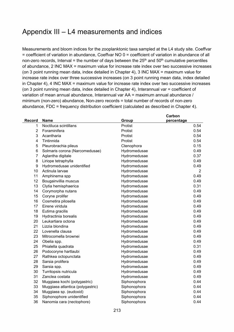
213
Appendix III – L4 measurements and indices
Measurements and bloom indices for the zooplanktonic taxa sampled at the L4 study site. Coeffvar= coefficient of variation in abundance, Coeffvar NO 0 = coefficient of variation in abundance of allnon-zero records, Interval = the number of days between the 25th and 50th cumulative percentilesof abundance, 2 INC MAX = maximum value for increase rate index over two successive increases(on 3 point running mean data, index detailed in Chapter 4), 3 INC MAX = maximum value forincrease rate index over three successive increases (on 3 point running mean data, index detailedin Chapter 4), 4 INC MAX = maximum value for increase rate index over two successive increases(on 3 point running mean data, index detailed in Chapter 4), Interannual var = coefficient ofvariation of mean annual abundance, Interannual var AA = maximum annual abundance /minimum (non-zero) abundance, Non-zero records = total number of records of non-zeroabundance, FDC = frequency distribution coefficient (calculated as described in Chapter 4).
Record Name GroupCarbonpercentage
1 Noctiluca scintillans Protist 0.542 Foraminifera Protist 0.543 Acantharia Protist 0.544 Tintinnida Protist 0.545 Pleurobrachia pileus Ctenophora 0.156 Solmaris corona (Narcomedusae) Hydromedusae 0.497 Aglantha digitale Hydromedusae 0.378 Liriope tetraphylla Hydromedusae 0.499 Hydromedusae unidentified Hydromedusae 0.4910 Actinula larvae Hydromedusae 211 Amphinema spp Hydromedusae 0.4912 Bougainvillia muscus Hydromedusae 0.4913 Clytia hemisphaerica Hydromedusae 0.3114 Corymorpha nutans Hydromedusae 0.4915 Coryne prolifer Hydromedusae 0.4916 Cosmetira pilosella Hydromedusae 0.4917 Eirene viridula Hydromedusae 0.4918 Eutima gracilis Hydromedusae 0.4919 Hydractinia borealis Hydromedusae 0.4920 Leukartiara octona Hydromedusae 0.4921 Lizzia blondina Hydromedusae 0.4922 Lovenella clausa Hydromedusae 0.4923 Mitrocomella brownei Hydromedusae 0.4924 Obelia spp. Hydromedusae 0.4925 Phialella quadrata Hydromedusae 0.3126 Podocoryne hartlaubi Hydromedusae 0.4927 Rathkea octopunctata Hydromedusae 0.4928 Sarsia prolifera Hydromedusae 0.4929 Sarsia spp. Hydromedusae 0.4930 Turritopsis nutricula Hydromedusae 0.4931 Zanclea costata Hydromedusae 0.4932 Muggiaea kochi (polygastric) Siphonophora 0.4433 Muggiaea atlantica (polygastric) Siphonophora 0.4434 Muggiaea sp. (eudoxid) Siphonophora 0.4435 Siphonophore unidentified Siphonophora 0.4436 Nanomia cara (nectophore) Siphonophora 0.44
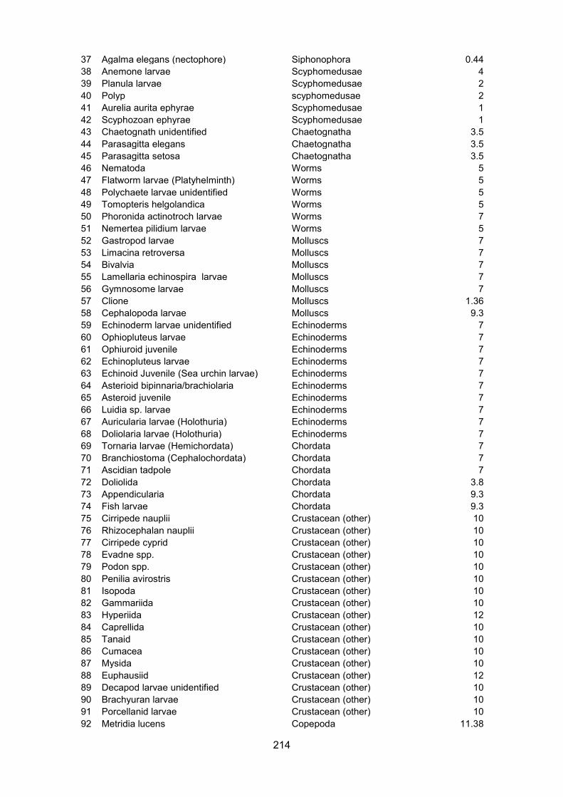
214
37 Agalma elegans (nectophore) Siphonophora 0.4438 Anemone larvae Scyphomedusae 439 Planula larvae Scyphomedusae 240 Polyp scyphomedusae 241 Aurelia aurita ephyrae Scyphomedusae 142 Scyphozoan ephyrae Scyphomedusae 143 Chaetognath unidentified Chaetognatha 3.544 Parasagitta elegans Chaetognatha 3.545 Parasagitta setosa Chaetognatha 3.546 Nematoda Worms 547 Flatworm larvae (Platyhelminth) Worms 548 Polychaete larvae unidentified Worms 549 Tomopteris helgolandica Worms 550 Phoronida actinotroch larvae Worms 751 Nemertea pilidium larvae Worms 552 Gastropod larvae Molluscs 753 Limacina retroversa Molluscs 754 Bivalvia Molluscs 755 Lamellaria echinospira larvae Molluscs 756 Gymnosome larvae Molluscs 757 Clione Molluscs 1.3658 Cephalopoda larvae Molluscs 9.359 Echinoderm larvae unidentified Echinoderms 760 Ophiopluteus larvae Echinoderms 761 Ophiuroid juvenile Echinoderms 762 Echinopluteus larvae Echinoderms 763 Echinoid Juvenile (Sea urchin larvae) Echinoderms 764 Asterioid bipinnaria/brachiolaria Echinoderms 765 Asteroid juvenile Echinoderms 766 Luidia sp. larvae Echinoderms 767 Auricularia larvae (Holothuria) Echinoderms 768 Doliolaria larvae (Holothuria) Echinoderms 769 Tornaria larvae (Hemichordata) Chordata 770 Branchiostoma (Cephalochordata) Chordata 771 Ascidian tadpole Chordata 772 Doliolida Chordata 3.873 Appendicularia Chordata 9.374 Fish larvae Chordata 9.375 Cirripede nauplii Crustacean (other) 1076 Rhizocephalan nauplii Crustacean (other) 1077 Cirripede cyprid Crustacean (other) 1078 Evadne spp. Crustacean (other) 1079 Podon spp. Crustacean (other) 1080 Penilia avirostris Crustacean (other) 1081 Isopoda Crustacean (other) 1082 Gammariida Crustacean (other) 1083 Hyperiida Crustacean (other) 1284 Caprellida Crustacean (other) 1085 Tanaid Crustacean (other) 1086 Cumacea Crustacean (other) 1087 Mysida Crustacean (other) 1088 Euphausiid Crustacean (other) 1289 Decapod larvae unidentified Crustacean (other) 1090 Brachyuran larvae Crustacean (other) 1091 Porcellanid larvae Crustacean (other) 1092 Metridia lucens Copepoda 11.38
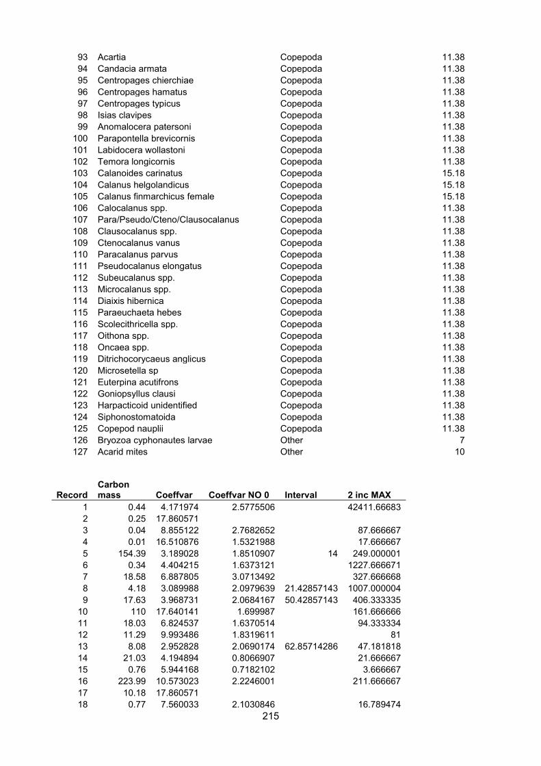
215
93 Acartia Copepoda 11.3894 Candacia armata Copepoda 11.3895 Centropages chierchiae Copepoda 11.3896 Centropages hamatus Copepoda 11.3897 Centropages typicus Copepoda 11.3898 Isias clavipes Copepoda 11.3899 Anomalocera patersoni Copepoda 11.38100 Parapontella brevicornis Copepoda 11.38101 Labidocera wollastoni Copepoda 11.38102 Temora longicornis Copepoda 11.38103 Calanoides carinatus Copepoda 15.18104 Calanus helgolandicus Copepoda 15.18105 Calanus finmarchicus female Copepoda 15.18106 Calocalanus spp. Copepoda 11.38107 Para/Pseudo/Cteno/Clausocalanus Copepoda 11.38108 Clausocalanus spp. Copepoda 11.38109 Ctenocalanus vanus Copepoda 11.38110 Paracalanus parvus Copepoda 11.38111 Pseudocalanus elongatus Copepoda 11.38112 Subeucalanus spp. Copepoda 11.38113 Microcalanus spp. Copepoda 11.38114 Diaixis hibernica Copepoda 11.38115 Paraeuchaeta hebes Copepoda 11.38116 Scolecithricella spp. Copepoda 11.38117 Oithona spp. Copepoda 11.38118 Oncaea spp. Copepoda 11.38119 Ditrichocorycaeus anglicus Copepoda 11.38120 Microsetella sp Copepoda 11.38121 Euterpina acutifrons Copepoda 11.38122 Goniopsyllus clausi Copepoda 11.38123 Harpacticoid unidentified Copepoda 11.38124 Siphonostomatoida Copepoda 11.38125 Copepod nauplii Copepoda 11.38126 Bryozoa cyphonautes larvae Other 7127 Acarid mites Other 10
RecordCarbonmass Coeffvar Coeffvar NO 0 Interval 2 inc MAX
1 0.44 4.171974 2.5775506 42411.666832 0.25 17.8605713 0.04 8.855122 2.7682652 87.6666674 0.01 16.510876 1.5321988 17.6666675 154.39 3.189028 1.8510907 14 249.0000016 0.34 4.404215 1.6373121 1227.6666717 18.58 6.887805 3.0713492 327.6666688 4.18 3.089988 2.0979639 21.42857143 1007.0000049 17.63 3.968731 2.0684167 50.42857143 406.33333510 110 17.640141 1.699987 161.66666611 18.03 6.824537 1.6370514 94.33333412 11.29 9.993486 1.8319611 8113 8.08 2.952828 2.0690174 62.85714286 47.18181814 21.03 4.194894 0.8066907 21.66666715 0.76 5.944168 0.7182102 3.66666716 223.99 10.573023 2.2246001 211.66666717 10.18 17.86057118 0.77 7.560033 2.1030846 16.789474
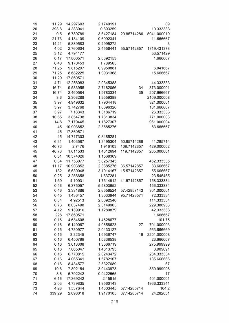
216
19 11.29 14.297603 2.1740191 8920 393.8 4.383941 0.893259 10.33333321 0.5 6.789789 3.6427184 20.85714286 5041.00001922 21.73 4.134109 0.6992341 11.66666723 14.21 5.889583 0.4995272 324 4.02 2.760604 2.4556441 55.57142857 1319.43137825 3.12 4.794177 53.57142926 0.17 17.860571 2.0392153 1.66666727 6.48 9.170453 1.78956528 71.25 9.815297 0.9950881 6.04166729 71.25 8.682225 1.9931368 15.66666730 11.29 17.86057131 4.71 12.256083 2.0345388 44.33333332 16.74 9.583955 2.7182056 34 373.00000133 16.74 2.460584 1.9783334 35 207.66666734 3.6 2.303288 1.9559388 2109.00000835 3.97 4.949632 1.7904418 321.00000136 3.97 3.742768 1.6696326 131.66666737 3.97 7.18343 1.3186719 26.33333338 10.55 3.854738 1.7613834 771.00000339 14.8 7.179445 1.1827307 961.00000440 45 10.903852 2.3885276 83.66666741 45 17.86057142 45 14.717303 0.848528143 6.31 1.403587 1.3495304 50.85714286 41.28571444 46.73 2.7476 1.916103 108.7142857 429.00000245 46.73 1.611533 1.4612694 119.7142857 265.00000146 0.31 10.574026 1.156836947 0.34 11.753077 3.8257343 462.33333548 11.17 10.903852 2.3885276 36.57142857 83.66666749 182 5.630048 3.1014167 15.57142857 55.66666750 0.25 3.256658 1.537281 23.54545551 1.59 4.10931 1.7514912 41.57142857 158.33333452 0.46 6.375057 5.5803652 156.33333453 0.46 3.331886 2.6556524 57.42857143 301.00000154 0.45 1.436457 1.3033944 95.71428571 72.33333455 0.34 4.92513 2.0092546 114.33333456 0.73 8.057498 2.3149905 229.38095357 4.12 9.139916 1.1280879 42.33333358 228 17.860571 1.66666759 0.16 4.634608 1.4628677 101.7560 0.16 6.140067 4.0658623 27 701.00000361 0.16 4.730977 2.0433127 563.66666962 0.16 3.32345 1.6936747 16 2201.00000863 0.16 6.450789 1.0338538 23.66666764 0.16 3.613308 1.3566719 275.99999965 0.16 7.065047 1.4613795 3.90909166 0.16 6.770815 2.0243472 234.33333467 0.16 4.065341 1.5782107 185.66666668 0.16 8.434577 2.5327689 6769 19.6 7.892154 3.0443973 850.99999870 8.6 5.792242 0.9422565 1771 6.16 17.369242 2.15915 401.00000172 2.03 4.739835 1.9560143 1966.33334173 4.28 1.537644 1.4603445 57.14285714 104.274 339.29 2.098018 1.9170105 37.14285714 24.282051
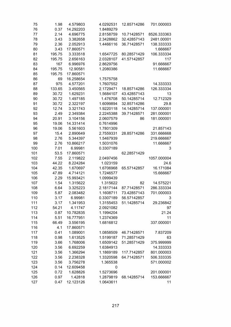
217
75 1.98 4.579803 4.0292531 12.85714286 701.00000376 0.37 14.292203 1.848927977 2.14 4.696775 2.8158759 10.71428571 8526.33336378 3.43 3.382658 2.3428862 32.42857143 2481.0000179 2.36 2.052913 1.4466116 36.71428571 138.33333380 3.43 17.860571 1.66666781 195.75 3.333518 1.6547725 80.28571429 106.33333482 195.75 2.656163 2.0328107 41.57142857 11783 167 6.996976 2.8629756 91.66666784 195.75 12.90581 1.2080386 11.66666785 195.75 17.86057186 69 16.258654 1.757575887 975 4.577201 1.7607552 14.33333388 133.65 3.450565 2.1729471 18.85714286 126.33333489 30.72 1.629231 1.5684107 43.42857143 1390 30.72 1.497185 1.476708 50.14285714 12.71232991 30.72 2.322197 1.6099894 32.85714286 29.892 12.74 3.321743 1.9220118 14.14285714 137.00000193 2.49 2.349384 2.2245388 39.71428571 281.00000194 20.91 3.104156 2.0607579 86 181.00000195 19.06 14.331414 0.761499696 19.06 5.561603 1.7801309 21.85714397 15.4 2.890649 2.7559331 28.85714286 331.66666898 2.76 5.344397 1.5467939 219.66666799 2.76 10.866217 1.5031076 11.666667100 7.01 6.99981 0.3307189 3101 53.5 17.860571 62.28571429102 7.55 2.119822 2.0497456 1057.000004103 44.22 8.224284 1.023159 24.6104 42.35 1.670697 1.6706968 65.57142857 16.171084105 47.89 4.714121 1.7246577 15.666667106 2.29 15.993421 1.0999439107 1.54 1.315622 1.315622 82 14.575221108 6.64 3.325223 2.1817144 87.71428571 286.333334109 5.87 2.083482 1.1608711 73.42857143 701.000003110 3.17 6.99981 0.3307189 56.57142857 3111 3.17 1.341953 1.3155453 51.14285714 29.236842112 54.21 4.11747 2.0921082 97113 0.87 10.782835 1.1994204 21.24114 5.51 16.777951 1.2374369 11115 66.49 3.556195 1.6816812 337.000001116 4.1 17.860571117 0.41 1.089001 1.0858509 46.71428571 7.837209118 0.98 1.613525 1.5199187 71.28571429 63119 3.66 1.768006 1.6509142 51.28571429 375.999999120 3.56 6.692259 1.6384913 14.333333121 3.56 1.366294 1.1869189 117.7142857 801.000003122 3.56 2.238328 1.3320598 64.71428571 506.333335123 3.56 3.756278 1.365538 571.000002124 0.14 12.609458 0125 0.72 1.628826 1.5273696 201.000001126 0.97 1.42818 1.2879819 68.14285714 153.666667127 0.47 12.123126 1.0643611 11
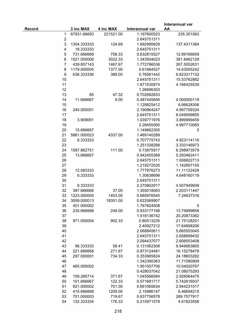
218
Record 3 inc MAX 4 inc MAX Interannual varInterannual varAA
1 67931.66693 221521.00 1.197800523 235.3515832 2.6457513113 1304.333333 124.69 1.692990629 137.43113844 18.333333 2.6457513115 731.666669 758.33 0.632815527 12.891666596 1521.000006 3022.33 1.343504023 381.84621297 439.857143 1467.67 1.772786536 267.50526318 1179.000005 1377.00 0.61664527 14.635552429 636.333336 389.00 0.76561442 6.82331713210 2.645751311 15.5376288211 1.871530874 4.16642553912 1.2669630313 85 47.32 0.70268283314 11.666667 9.00 0.487445695 4.00000011915 1.128825412 6.6662830616 245.000001 2.190864247 4.99770932417 2.645751311 8.04959985518 3.909091 1.039771976 3.89999945919 2.28455065 4.99771006520 15.666667 1.149662305 521 5861.000023 4337.00 1.46914028822 6.333333 0.707775743 4.92311411623 1.251338288 3.33314697324 1597.862751 111.00 0.73875917 6.29897357925 13.666667 0.942455389 5.29346241126 2.645751311 1.93682271327 1.219272535 1.14285715528 12.083333 1.777876273 11.1112242829 6.333333 1.30638698 4.64816011930 2.64575131131 8.333333 2.270802917 4.50794993832 387.666668 37.00 1.355018083 2.20311144733 1223.000005 1403.00 0.685976545 7.2463731634 3559.000013 18351.00 0.62206990735 401.000002 1.767824508 536 235.666668 249.00 0.933177166 13.7999985837 1.518136742 20.2087338238 971.000004 902.33 0.80513235 21.7512820139 2.40927212 17.6489820640 2.068845611 5.66555304541 2.645751311 2.65869943242 2.094437077 2.60655340843 96.333333 58.41 0.131062308 9.94906380544 221.666668 271.67 0.873124481 16.1527847845 297.000001 734.33 0.353985824 24.1860328246 1.342390363 11.7159090947 465.000002 1.951507706 10.0402076748 0.428037042 21.0807529349 159.285714 371.67 1.045566084 2.92656447550 101.666667 122.33 0.571681717 5.74261603751 621.000002 701.00 0.661065634 2.94423151752 415.666668 1209.00 2.15986147 6.4669421553 701.000003 719.67 0.637756578 269.757791754 132.333334 176.33 0.215971578 4.61823558
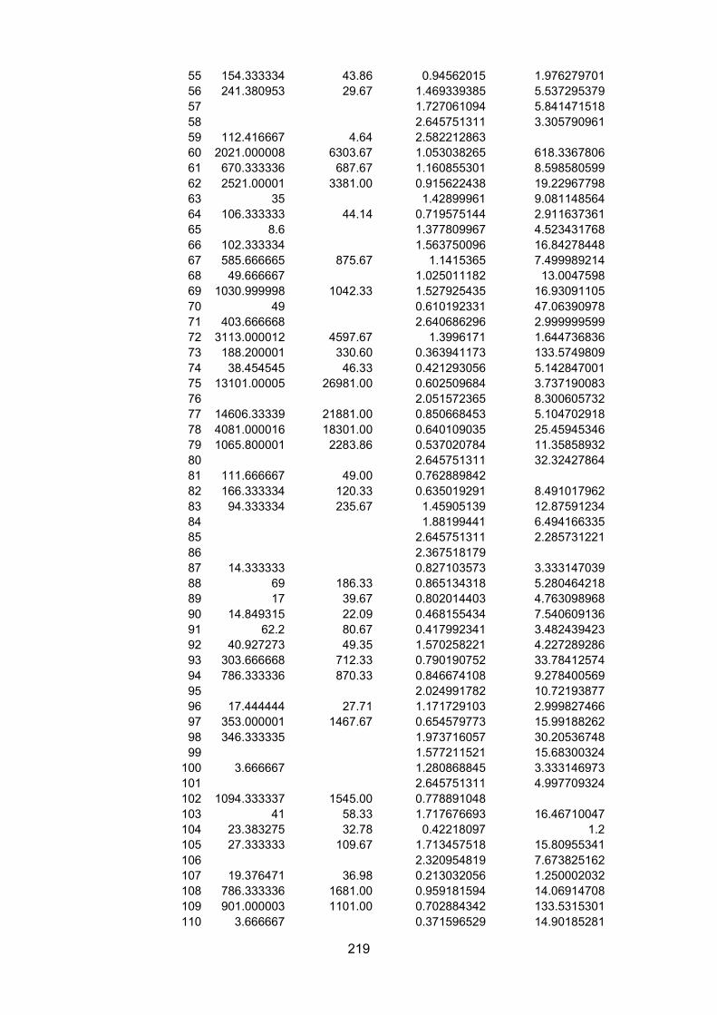
219
55 154.333334 43.86 0.94562015 1.97627970156 241.380953 29.67 1.469339385 5.53729537957 1.727061094 5.84147151858 2.645751311 3.30579096159 112.416667 4.64 2.58221286360 2021.000008 6303.67 1.053038265 618.336780661 670.333336 687.67 1.160855301 8.59858059962 2521.00001 3381.00 0.915622438 19.2296779863 35 1.42899961 9.08114856464 106.333333 44.14 0.719575144 2.91163736165 8.6 1.377809967 4.52343176866 102.333334 1.563750096 16.8427844867 585.666665 875.67 1.1415365 7.49998921468 49.666667 1.025011182 13.004759869 1030.999998 1042.33 1.527925435 16.9309110570 49 0.610192331 47.0639097871 403.666668 2.640686296 2.99999959972 3113.000012 4597.67 1.3996171 1.64473683673 188.200001 330.60 0.363941173 133.574980974 38.454545 46.33 0.421293056 5.14284700175 13101.00005 26981.00 0.602509684 3.73719008376 2.051572365 8.30060573277 14606.33339 21881.00 0.850668453 5.10470291878 4081.000016 18301.00 0.640109035 25.4594534679 1065.800001 2283.86 0.537020784 11.3585893280 2.645751311 32.3242786481 111.666667 49.00 0.76288984282 166.333334 120.33 0.635019291 8.49101796283 94.333334 235.67 1.45905139 12.8759123484 1.88199441 6.49416633585 2.645751311 2.28573122186 2.36751817987 14.333333 0.827103573 3.33314703988 69 186.33 0.865134318 5.28046421889 17 39.67 0.802014403 4.76309896890 14.849315 22.09 0.468155434 7.54060913691 62.2 80.67 0.417992341 3.48243942392 40.927273 49.35 1.570258221 4.22728928693 303.666668 712.33 0.790190752 33.7841257494 786.333336 870.33 0.846674108 9.27840056995 2.024991782 10.7219387796 17.444444 27.71 1.171729103 2.99982746697 353.000001 1467.67 0.654579773 15.9918826298 346.333335 1.973716057 30.2053674899 1.577211521 15.68300324100 3.666667 1.280868845 3.333146973101 2.645751311 4.997709324102 1094.333337 1545.00 0.778891048103 41 58.33 1.717676693 16.46710047104 23.383275 32.78 0.42218097 1.2105 27.333333 109.67 1.713457518 15.80955341106 2.320954819 7.673825162107 19.376471 36.98 0.213032056 1.250002032108 786.333336 1681.00 0.959181594 14.06914708109 901.000003 1101.00 0.702884342 133.5315301110 3.666667 0.371596529 14.90185281
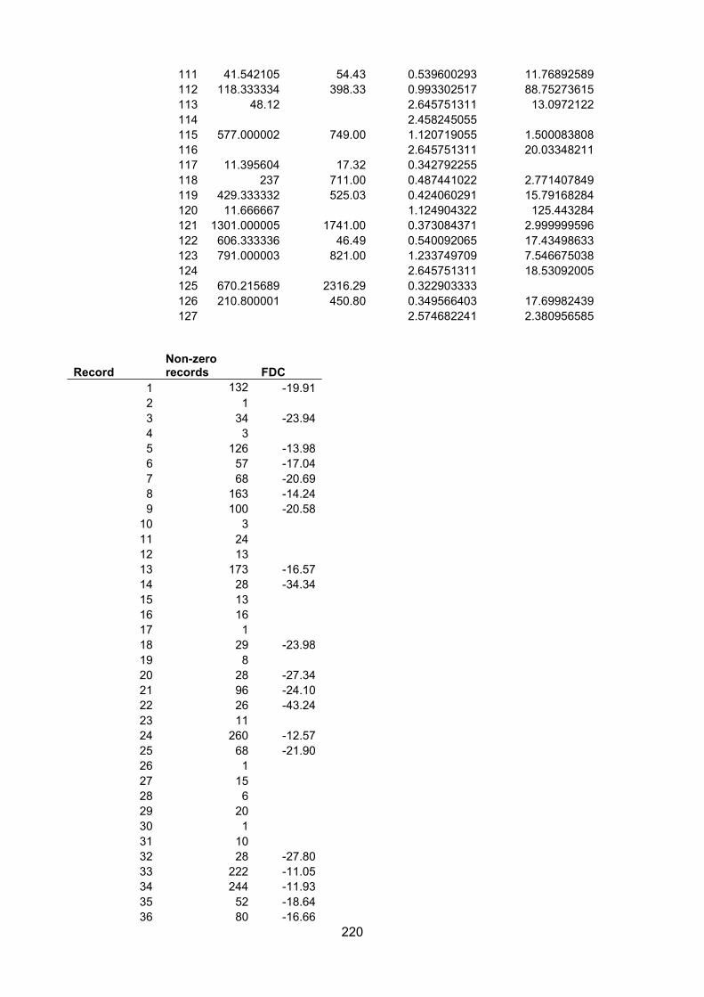
220
111 41.542105 54.43 0.539600293 11.76892589112 118.333334 398.33 0.993302517 88.75273615113 48.12 2.645751311 13.0972122114 2.458245055115 577.000002 749.00 1.120719055 1.500083808116 2.645751311 20.03348211117 11.395604 17.32 0.342792255118 237 711.00 0.487441022 2.771407849119 429.333332 525.03 0.424060291 15.79168284120 11.666667 1.124904322 125.443284121 1301.000005 1741.00 0.373084371 2.999999596122 606.333336 46.49 0.540092065 17.43498633123 791.000003 821.00 1.233749709 7.546675038124 2.645751311 18.53092005125 670.215689 2316.29 0.322903333126 210.800001 450.80 0.349566403 17.69982439127 2.574682241 2.380956585
RecordNon-zerorecords FDC
1 132 -19.912 13 34 -23.944 35 126 -13.986 57 -17.047 68 -20.698 163 -14.249 100 -20.5810 311 2412 1313 173 -16.5714 28 -34.3415 1316 1617 118 29 -23.9819 820 28 -27.3421 96 -24.1022 26 -43.2423 1124 260 -12.5725 68 -21.9026 127 1528 629 2030 131 1032 28 -27.8033 222 -11.0534 244 -11.9335 52 -18.6436 80 -16.66
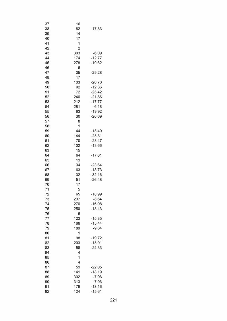
221
37 1638 82 -17.3339 1440 1741 142 243 303 -6.0944 174 -12.7745 278 -10.6246 647 35 -29.2848 1749 103 -20.7050 92 -12.3651 72 -23.4252 246 -21.8653 212 -17.7754 281 -6.1855 63 -19.9256 30 -26.6957 858 159 44 -15.4960 144 -23.3161 70 -23.4762 102 -13.6663 1564 64 -17.6165 1966 34 -23.6467 63 -18.7368 32 -32.1669 51 -26.4870 1771 572 65 -18.9973 297 -8.6474 276 -16.0875 250 -18.4376 677 123 -15.3578 166 -15.4479 189 -9.6480 181 98 -19.7282 203 -13.9183 58 -24.3384 485 186 487 59 -22.0588 141 -18.1989 302 -7.9690 313 -7.9391 179 -13.1692 124 -15.61
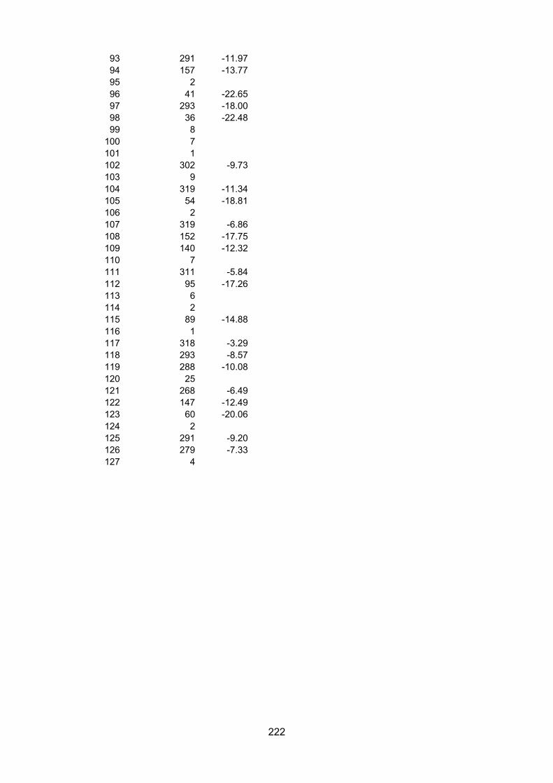
222
93 291 -11.9794 157 -13.7795 296 41 -22.6597 293 -18.0098 36 -22.4899 8100 7101 1102 302 -9.73103 9104 319 -11.34105 54 -18.81106 2107 319 -6.86108 152 -17.75109 140 -12.32110 7111 311 -5.84112 95 -17.26113 6114 2115 89 -14.88116 1117 318 -3.29118 293 -8.57119 288 -10.08120 25121 268 -6.49122 147 -12.49123 60 -20.06124 2125 291 -9.20126 279 -7.33127 4

223
Appendix IV – Published work
Permission to reproduce this article has been granted by Oxford University Press
Journal of
Plankton Research plankt.oxfordjournals.org
J. Plankton Res. (2016) 00(00): 1–11. doi:10.1093/plankt/fbw094
Disentangling the counteracting effectsof water content and carbon masson zooplankton growth
KRISTIAN MCCONVILLE1,2*, ANGUS ATKINSON1, ELAINE S. FILEMAN1, JOHN I. SPICER2 AND ANDREW G. HIRST3,4
PLYMOUTH MARINE LABORATORY, PROSPECT PLACE, PLYMOUTH PL DH, UNITED KINGDOM, MARINE BIOLOGY & ECOLOGY RESEARCH CENTRE, SCHOOL OF
MARINE SCIENCE & ENGINEERING, PLYMOUTH UNIVERSITY, DRAKE’S CIRCUS, PLYMOUTH PL AA, UNITED KINGDOM, SCHOOL OF BIOLOGICAL AND
CHEMICAL SCIENCES, QUEEN MARY UNIVERSITY OF LONDON, MILE END ROAD, LONDON E NS, UNITED KINGDOM ANDCENTRE FOR OCEAN LIFE, NATIONAL
INSTITUTE FOR AQUATIC RESOURCES, TECHNICAL UNIVERSITY OF DENMARK, KAVALERGARDEN , CHARLOTTENLUND , DENMARK
*CORRESPONDING AUTHOR: [email protected]
Received February 26, 2016; editorial decision November 30, 2016; accepted December 12, 2016
Corresponding editor: Marja Koski
Zooplankton vary widely in carbon percentage (carbon mass as a percentage of wet mass), but are often describedas either gelatinous or non-gelatinous. Here we update datasets of carbon percentage and growth rate to investigatewhether carbon percentage is a continuous trait, and whether its inclusion improves zooplankton growth models.We found that carbon percentage is continuous, but that species are not distributed homogenously along this axis.To assess variability of this trait in situ, we investigated the distribution of biomass across the range of carbon per-centage for a zooplankton time series at station L4 off Plymouth, UK. This showed separate biomass peaks for gel-atinous and crustacean taxa, however, carbon percentage varied 8-fold within the gelatinous group. Species withhigh carbon mass had lower carbon percentage, allowing separation of the counteracting effects of these two vari-ables on growth rate. Specific growth rates, g (d−1) were negatively related to carbon percentage and carbon mass,even in the gelatinous taxa alone, suggesting that the trend is not driven by a categorical difference between thesegroups. The addition of carbon percentage doubled the explanatory power of growth models based on mass alone,demonstrating the benefits of considering carbon percentage as a continuous trait.
KEYWORDS: water content; zooplankton; gelatinous; carbon percentage; growth
INTRODUCTION
Gelatinous zooplankton are a phylogenetically broad andecologically important group of taxa found throughout
the world’s oceans. Their prey range from bacteria to fish(Sutherland et al., 2010) and they exhibit an equallydiverse range of life history strategies and body composi-tions. The high water content characteristic of this group
available online at www.plankt.oxfordjournals.org
© The Author 2016. Published by Oxford University Press. All rights reserved. For permissions, please e-mail: [email protected]
JPR Advance Access published December 29, 2016 at T
he Marine B
iological Association of the U
K on January 4, 2017
http://plankt.oxfordjournals.org/D
ownloaded from
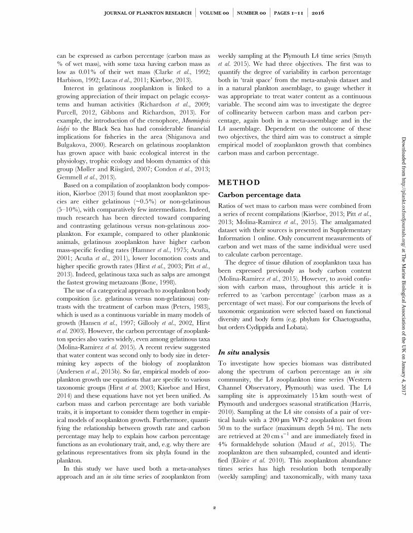
can be expressed as carbon percentage (carbon mass as% of wet mass), with some taxa having carbon mass aslow as 0.01% of their wet mass (Clarke et al., 1992;Harbison, 1992; Lucas et al., 2011; Kiørboe, 2013).
Interest in gelatinous zooplankton is linked to agrowing appreciation of their impact on pelagic ecosys-tems and human activities (Richardson et al., 2009;Purcell, 2012, Gibbons and Richardson, 2013). Forexample, the introduction of the ctenophore, Mnemiopsis
leidyi to the Black Sea has had considerable financialimplications for fisheries in the area (Shiganova andBulgakova, 2000). Research on gelatinous zooplanktonhas grown apace with basic ecological interest in thephysiology, trophic ecology and bloom dynamics of thisgroup (Møller and Riisgård, 2007; Condon et al., 2013;Gemmell et al., 2013).
Based on a compilation of zooplankton body compos-ition, Kiørboe (2013) found that most zooplankton spe-cies are either gelatinous (~0.5%) or non-gelatinous(5–10%), with comparatively few intermediates. Indeed,much research has been directed toward comparingand contrasting gelatinous versus non-gelatinous zoo-plankton. For example, compared to other planktonicanimals, gelatinous zooplankton have higher carbonmass-specific feeding rates (Hamner et al., 1975; Acuña,2001; Acuña et al., 2011), lower locomotion costs andhigher specific growth rates (Hirst et al., 2003; Pitt et al.,2013). Indeed, gelatinous taxa such as salps are amongstthe fastest growing metazoans (Bone, 1998).
The use of a categorical approach to zooplankton bodycomposition (i.e. gelatinous versus non-gelatinous) con-trasts with the treatment of carbon mass (Peters, 1983),which is used as a continuous variable in many models ofgrowth (Hansen et al., 1997; Gillooly et al., 2002, Hirstet al. 2003). However, the carbon percentage of zooplank-ton species also varies widely, even among gelatinous taxa(Molina-Ramirez et al. 2015). A recent review suggestedthat water content was second only to body size in deter-mining key aspects of the biology of zooplankton(Andersen et al., 2015b). So far, empirical models of zoo-plankton growth use equations that are specific to varioustaxonomic groups (Hirst et al. 2003; Kiørboe and Hirst,2014) and these equations have not yet been unified. Ascarbon mass and carbon percentage are both variabletraits, it is important to consider them together in empir-ical models of zooplankton growth. Furthermore, quanti-fying the relationship between growth rate and carbonpercentage may help to explain how carbon percentagefunctions as an evolutionary trait, and, e.g. why there aregelatinous representatives from six phyla found in theplankton.
In this study we have used both a meta-analysesapproach and an in situ time series of zooplankton from
weekly sampling at the Plymouth L4 time series (Smythet al. 2015). We had three objectives. The first was toquantify the degree of variability in carbon percentageboth in ‘trait space’ from the meta-analysis dataset andin a natural plankton assemblage, to gauge whether itwas appropriate to treat water content as a continuousvariable. The second aim was to investigate the degreeof collinearity between carbon mass and carbon per-centage, again both in a meta-assemblage and in theL4 assemblage. Dependent on the outcome of thesetwo objectives, the third aim was to construct a simpleempirical model of zooplankton growth that combinescarbon mass and carbon percentage.
METHOD
Carbon percentage data
Ratios of wet mass to carbon mass were combined froma series of recent compilations (Kiørboe, 2013; Pitt et al.,2013; Molina-Ramirez et al., 2015). The amalgamateddataset with their sources is presented in SupplementaryInformation 1 online. Only concurrent measurements ofcarbon and wet mass of the same individual were usedto calculate carbon percentage.The degree of tissue dilution of zooplankton taxa has
been expressed previously as body carbon content(Molina-Ramirez et al., 2015). However, to avoid confu-sion with carbon mass, throughout this article it isreferred to as ‘carbon percentage’ (carbon mass as apercentage of wet mass). For our comparisons the levels oftaxonomic organization were selected based on functionaldiversity and body form (e.g. phylum for Chaetognatha,but orders Cydippida and Lobata).
In situ analysis
To investigate how species biomass was distributedalong the spectrum of carbon percentage an in situ
community, the L4 zooplankton time series (WesternChannel Observatory, Plymouth) was used. The L4sampling site is approximately 15 km south–west ofPlymouth and undergoes seasonal stratification (Harris,2010). Sampling at the L4 site consists of a pair of ver-tical hauls with a 200 µm WP-2 zooplankton net from50 m to the surface (maximum depth 54 m). The netsare retrieved at 20 cm s−1 and are immediately fixed in4% formaldehyde solution (Maud et al., 2015). Thezooplankton are then subsampled, counted and identi-fied (Eloire et al. 2010). This zooplankton abundancetimes series has high resolution both temporally(weekly sampling) and taxonomically, with many taxa
JOURNAL OF PLANKTON RESEARCH j VOLUME j NUMBER j PAGES – j at T
he Marine B
iological Association of the U
K on January 4, 2017
http://plankt.oxfordjournals.org/D
ownloaded from
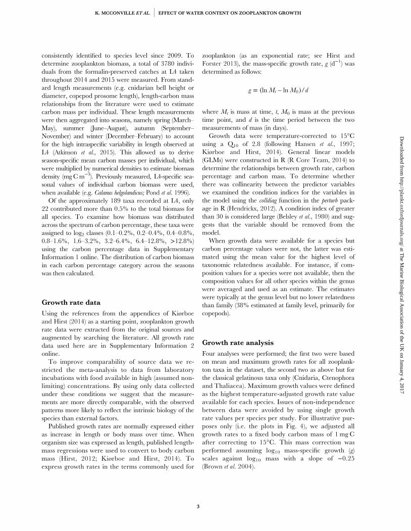
consistently identified to species level since 2009. Todetermine zooplankton biomass, a total of 3780 indivi-duals from the formalin-preserved catches at L4 takenthroughout 2014 and 2015 were measured. From stand-ard length measurements (e.g. cnidarian bell height ordiameter, copepod prosome length), length-carbon massrelationships from the literature were used to estimatecarbon mass per individual. These length measurementswere then aggregated into seasons, namely spring (March–May), summer (June–August), autumn (September–November) and winter (December–February) to accountfor the high intraspecific variability in length observed atL4 (Atkinson et al., 2015). This allowed us to deriveseason-specific mean carbon masses per individual, whichwere multiplied by numerical densities to estimate biomassdensity (mgCm−3). Previously measured, L4-specific sea-sonal values of individual carbon biomass were used,when available (e.g. Calanus helgolandicus; Pond et al. 1996).Of the approximately 189 taxa recorded at L4, only
22 contributed more than 0.5% to the total biomass forall species. To examine how biomass was distributedacross the spectrum of carbon percentage, these taxa wereassigned to log2 classes (0.1–0.2%, 0.2–0.4%, 0.4–0.8%,0.8–1.6%, 1.6–3.2%, 3.2–6.4%, 6.4–12.8%, >12.8%)using the carbon percentage data in SupplementaryInformation 1 online. The distribution of carbon biomassin each carbon percentage category across the seasonswas then calculated.
Growth rate data
Using the references from the appendices of Kiørboeand Hirst (2014) as a starting point, zooplankton growthrate data were extracted from the original sources andaugmented by searching the literature. All growth ratedata used here are in Supplementary Information 2online.To improve comparability of source data we re-
stricted the meta-analysis to data from laboratoryincubations with food available in high (assumed non-limiting) concentrations. By using only data collectedunder these conditions we suggest that the measure-ments are more directly comparable, with the observedpatterns more likely to reflect the intrinsic biology of thespecies than external factors.Published growth rates are normally expressed either
as increase in length or body mass over time. Whenorganism size was expressed as length, published length-mass regressions were used to convert to body carbonmass (Hirst, 2012; Kiørboe and Hirst, 2014). Toexpress growth rates in the terms commonly used for
zooplankton (as an exponential rate; see Hirst andForster 2013), the mass-specific growth rate, g (d−1) wasdetermined as follows:
= ( – )g M M dln ln /t 0
where Mt is mass at time, t, M0 is mass at the previoustime point, and d is the time period between the twomeasurements of mass (in days).
Growth data were temperature-corrected to 15°Cusing a Q10 of 2.8 (following Hansen et al., 1997;Kiørboe and Hirst, 2014). General linear models(GLMs) were constructed in R (R Core Team, 2014) todetermine the relationships between growth rate, carbonpercentage and carbon mass. To determine whetherthere was collinearity between the predictor variableswe examined the condition indices for the variables inthe model using the colldiag function in the perturb pack-age in R (Hendrickx, 2012). A condition index of greaterthan 30 is considered large (Belsley et al., 1980) and sug-gests that the variable should be removed from themodel.
When growth data were available for a species butcarbon percentage values were not, the latter was esti-mated using the mean value for the highest level oftaxonomic relatedness available. For instance, if com-position values for a species were not available, then thecomposition values for all other species within the genuswere averaged and used as an estimate. The estimateswere typically at the genus level but no lower relatednessthan family (38% estimated at family level, primarily forcopepods).
Growth rate analysis
Four analyses were performed; the first two were basedon mean and maximum growth rates for all zooplank-ton taxa in the dataset, the second two as above but forthe classical gelatinous taxa only (Cnidaria, Ctenophoraand Thaliacea). Maximum growth values were definedas the highest temperature-adjusted growth rate valueavailable for each species. Issues of non-independencebetween data were avoided by using single growthrate values per species per study. For illustrative pur-poses only (i.e. the plots in Fig. 4), we adjusted allgrowth rates to a fixed body carbon mass of 1 mg Cafter correcting to 15°C. This mass correction wasperformed assuming log10 mass-specific growth (g)scales against log10 mass with a slope of −0.25(Brown et al. 2004).
K. MCCONVILLE ET AL. j EFFECT OF WATER CONTENT ON ZOOPLANKTON GROWTH at T
he Marine B
iological Association of the U
K on January 4, 2017
http://plankt.oxfordjournals.org/D
ownloaded from
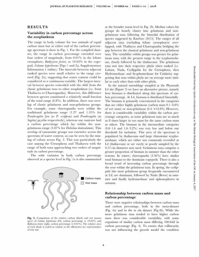
RESULTS
Variability in carbon percentage acrossthe zooplankton
The range in body volume for two animals of equalcarbon mass but at either end of the carbon percent-age spectrum is show in Fig. 1. For the compiled data-set, the range in carbon percentage extended overfour orders of magnitude, from 0.01% in the lobatectenophore, Bathycyroe fosteri, to 19.02% in the cope-pod, Calanus hyperboreus (Figs 1 and 2a, SupplementaryInformation 1 online). The intervals between adjacentranked species were small relative to the range cov-ered (Fig. 2a), suggesting that water content could beconsidered as a continuous variable. The largest inter-val between species coincided with the shift from theclassic gelatinous taxa to other zooplankton (i.e. fromThaliacea to Chaetognatha). However, this differencebetween species constituted a relatively small fractionof the total range (6.8%). In addition, there was over-lap of classic gelatinous and non-gelatinous groups.For example, some chaetognaths were within thetraditional gelatinous range (1.27 and 1.35% forPseudosagitta lyra (as P. scrippsae) and Pseudosagitta (asSagitta) gazellae respectively), whereas one tunicate hada carbon percentage which lay within the non-gelatinous range (3.87% for Doliolum denticulatum). Thisoverlap of taxonomic groups was extensive across thespectrum of water content, as can be seen by the mix-ing of colour across Fig. 2. This was particularly thecase among the Ctenophora and Thaliacea with therange of both taxa approaching two orders of magni-tude in carbon percentage.
The wide variation in body carbon percentageobserved at a species level in Fig. 1a is also summarized
at the broader taxon level in Fig. 2b. Median values forgroups do loosely cluster into gelatinous and non-gelatinous taxa following the bimodal distribution ofspecies suggested by Kiørboe (2013). The ranges of alladjacent taxa (excluding lobate ctenophores) over-lapped, with Thaliacea and Chaetognatha bridging thegap between the classical gelatinous and non-gelatinoustaxa. The variability within groups was greater for gelat-inous taxa, with the greatest range in the scyphomedu-sae, closely followed by the thaliaceans. The gelatinoustaxa sort into their respective phyla when ranked (i.e.Lobata, Nuda, Cydippida for the Ctenophora, thenHydromedusae and Scyphomedusae for Cnidaria) sug-gesting that taxa within phyla are on average more simi-lar to each other than with other phyla.In the natural assemblage sampled at the Plymouth
L4 site (Figure 3) we have an alternative picture, namelyhow biomass is distributed along this spectrum of car-bon percentage. At L4, biomass is distributed bimodally.The biomass is primarily concentrated in the categoriesthat are either highly gelatinous (carbon mass 0.1–0.8%of wet mass) or non-gelatinous (6.4–>12.8%) However,there is considerable variability within the carbon per-centage categories, as some gelatinous taxa are as muchas 8 times larger in wet mass for the same carbon massas others. The biomass in the intermediate categories(0.8–1.6 and 1.6–3.2%) was very low and below ourthreshold for inclusion. This area of the spectrum ispopulated by thaliaceans and large rhizostome scypho-medusae, which are either not commonly recorded atL4 (thaliaceans) or are rarely or poorly sampled by the0.57 cm diameter nets used. Gelatinous taxa comprise agreater proportion of biomass in summer than the otherseasons. In winter, chaetognaths (3.56%) have similartotal biomass to the dominant copepods. There is also abroad trend of increasing carbon percentage throughthe year within the gelatinous taxa. In spring, the cydip-pids (the most gelatinous group frequently encounteredat L4) are dominant, followed by Nuda (Beroe) in sum-mer and finally hydromedusae and siphonophores inautumn.
Relationship between carbon mass andcarbon percentage
There were negative relationships between carbon massand carbon percentage, both in the meta-dataset(Fig. 4a) and in the in situ dataset (Fig.4b). While themore gelatinous taxa tended to have higher carbonmass there was considerable variability, with someorganisms of similar carbon mass differing 100-fold incarbon percentage (Fig. 4). To ensure that collinearitywas not influencing the growth model the condition
Wet mass
Carbon mass
Fig. 1. Comparison of the relative carbon (black) and wet masses(grey) of Calanus hyperboreus (left, carbon percentage = 19.02%) andBathycyroe fosteri (right, carbon percentage = 0.01%). The relative areaof each shade is scaled as volume so the silhouettes are representativeof true size.
JOURNAL OF PLANKTON RESEARCH j VOLUME j NUMBER j PAGES – j at T
he Marine B
iological Association of the U
K on January 4, 2017
http://plankt.oxfordjournals.org/D
ownloaded from
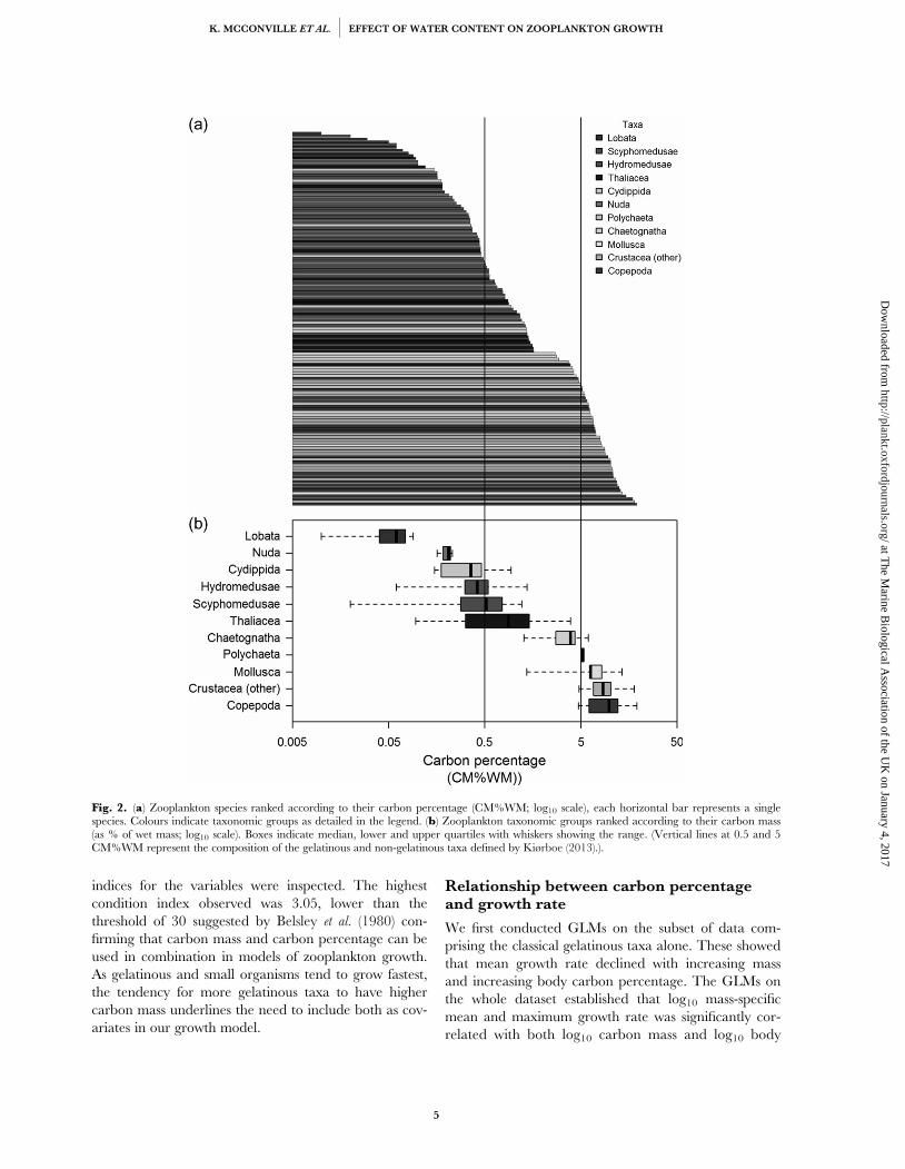
indices for the variables were inspected. The highestcondition index observed was 3.05, lower than thethreshold of 30 suggested by Belsley et al. (1980) con-firming that carbon mass and carbon percentage can beused in combination in models of zooplankton growth.As gelatinous and small organisms tend to grow fastest,the tendency for more gelatinous taxa to have highercarbon mass underlines the need to include both as cov-ariates in our growth model.
Relationship between carbon percentageand growth rate
We first conducted GLMs on the subset of data com-prising the classical gelatinous taxa alone. These showedthat mean growth rate declined with increasing massand increasing body carbon percentage. The GLMs onthe whole dataset established that log10 mass-specificmean and maximum growth rate was significantly cor-related with both log10 carbon mass and log10 body
Fig. 2. (a) Zooplankton species ranked according to their carbon percentage (CM%WM; log10 scale), each horizontal bar represents a singlespecies. Colours indicate taxonomic groups as detailed in the legend. (b) Zooplankton taxonomic groups ranked according to their carbon mass(as % of wet mass; log10 scale). Boxes indicate median, lower and upper quartiles with whiskers showing the range. (Vertical lines at 0.5 and 5CM%WM represent the composition of the gelatinous and non-gelatinous taxa defined by Kiørboe (2013).).
K. MCCONVILLE ET AL. j EFFECT OF WATER CONTENT ON ZOOPLANKTON GROWTH at T
he Marine B
iological Association of the U
K on January 4, 2017
http://plankt.oxfordjournals.org/D
ownloaded from
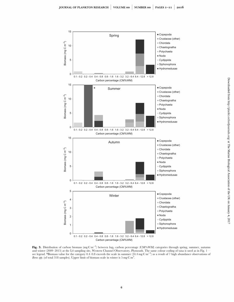
0
5
10
15
0.1 - 0.2 0.2 - 0.4 0.4 - 0.8 0.8 - 1.6 1.6 - 3.2 3.2 - 6.4 6.4 - 12.8 > 12.8
Bio
mass (
mg C
m–
3)
Carbon percentage (CM%WM)
Spring Copepoda
Crustacea (other)
Chordata
Chaetognatha
Polychaeta
Nuda
Cydippida
Siphonophora
Hydromedusae
0
5
10
15
0.1 - 0.2 0.2 - 0.4 0.4 - 0.8 0.8 - 1.6 1.6 - 3.2 3.2 - 6.4 6.4 - 12.8 > 12.8
Bio
mass (
mg C
m–
3)
Carbon percentage (CM%WM)
Summer Copepoda
Crustacea (other)
Chordata
Chaetognatha
Polychaeta
Nuda
Cydippida
Siphonophora
Hydromedusae
0
5
10
15
0.1 - 0.2 0.2 - 0.4 0.4 - 0.8 0.8 - 1.6 1.6 - 3.2 3.2 - 6.4 6.4 - 12.8 > 12.8
Bio
mass (
mg C
m–
3)
Carbon percentage (CM%WM)
Autumn Copepoda
Crustacea (other)
Chordata
Chaetognatha
Polychaeta
Nuda
Cydippida
Siphonophora
Hydromedusae
0
1
2
3
4
5
0.1 - 0.2 0.2 - 0.4 0.4 - 0.8 0.8 - 1.6 1.6 - 3.2 3.2 - 6.4 6.4 - 12.8 > 12.8
Bio
mass (
mg C
m–
3)
Carbon percentage (CM%WM)
WinterCopepoda
Crustacea (other)
Chordata
Chaetognatha
Polychaeta
Nuda
Cydippida
Siphonophora
Hydromedusae
*
Fig. 3. Distribution of carbon biomass (mg Cm−3) between log2 carbon percentage (CM%WM) categories through spring, summer, autumnand winter (2009–2015) at the L4 sampling site, Western Channel Observatory, Plymouth. The same colour coding of taxa is used as in Fig. 1—see legend. *Biomass value for the category 0.4–0.8 exceeds the scale in summer (34.4 mg Cm−3) as a result of 7 high abundance observations ofBeroe spp. (of total 318 samples). Upper limit of biomass scale in winter is 5 mg Cm3.
JOURNAL OF PLANKTON RESEARCH j VOLUME j NUMBER j PAGES – j at T
he Marine B
iological Association of the U
K on January 4, 2017
http://plankt.oxfordjournals.org/D
ownloaded from
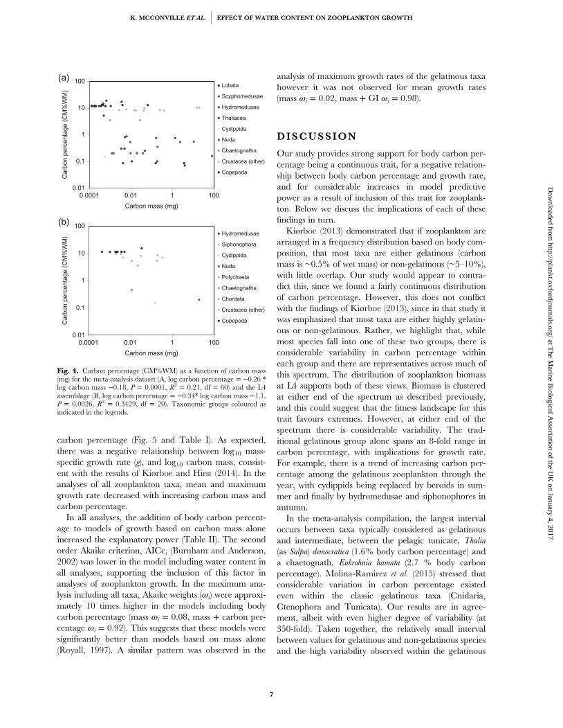
carbon percentage (Fig. 5 and Table I). As expected,there was a negative relationship between log10 mass-specific growth rate (g), and log10 carbon mass, consist-ent with the results of Kiørboe and Hirst (2014). In theanalyses of all zooplankton taxa, mean and maximumgrowth rate decreased with increasing carbon mass andcarbon percentage.In all analyses, the addition of body carbon percent-
age to models of growth based on carbon mass aloneincreased the explanatory power (Table II). The secondorder Akaike criterion, AICc, (Burnham and Anderson,2002) was lower in the model including water content inall analyses, supporting the inclusion of this factor inanalyses of zooplankton growth. In the maximum ana-lysis including all taxa, Akaike weights (ωi) were approxi-mately 10 times higher in the models including bodycarbon percentage (mass ωi = 0.08, mass + carbon per-centage ωi = 0.92). This suggests that these models weresignificantly better than models based on mass alone(Royall, 1997). A similar pattern was observed in the
analysis of maximum growth rates of the gelatinous taxahowever it was not observed for mean growth rates(mass ωi = 0.02, mass + GI ωi = 0.98).
DISCUSSION
Our study provides strong support for body carbon per-centage being a continuous trait, for a negative relation-ship between body carbon percentage and growth rate,and for considerable increases in model predictivepower as a result of inclusion of this trait for zooplank-ton. Below we discuss the implications of each of thesefindings in turn.
Kiørboe (2013) demonstrated that if zooplankton arearranged in a frequency distribution based on body com-position, that most taxa are either gelatinous (carbonmass is ~0.5% of wet mass) or non-gelatinous (~5–10%),with little overlap. Our study would appear to contra-dict this, since we found a fairly continuous distributionof carbon percentage. However, this does not conflictwith the findings of Kiørboe (2013), since in that study itwas emphasized that most taxa are either highly gelatin-ous or non-gelatinous. Rather, we highlight that, whilemost species fall into one of these two groups, there isconsiderable variability in carbon percentage withineach group and there are representatives across much ofthis spectrum. The distribution of zooplankton biomassat L4 supports both of these views. Biomass is clusteredat either end of the spectrum as described previously,and this could suggest that the fitness landscape for thistrait favours extremes. However, at either end of thespectrum there is considerable variability. The trad-itional gelatinous group alone spans an 8-fold range incarbon percentage, with implications for growth rate.For example, there is a trend of increasing carbon per-centage among the gelatinous zooplankton through theyear, with cydippids being replaced by beroids in sum-mer and finally by hydromedusae and siphonophores inautumn.
In the meta-analysis compilation, the largest intervaloccurs between taxa typically considered as gelatinousand intermediate, between the pelagic tunicate, Thalia(as Salpa) democratica (1.6% body carbon percentage) anda chaetognath, Eukrohnia hamata (2.7 % body carbonpercentage). Molina-Ramirez et al. (2015) stressed thatconsiderable variation in carbon percentage existedeven within the classic gelatinous taxa (Cnidaria,Ctenophora and Tunicata). Our results are in agree-ment, albeit with even higher degree of variability (at350-fold). Taken together, the relatively small intervalbetween values for gelatinous and non-gelatinous speciesand the high variability observed within the gelatinous
0.01
0.1
1
10
100
0.0001 0.01 1 100
Carb
on p
erc
enta
ge (
CM
%W
M)
Carbon mass (mg)
Lobata
Scyphomedusae
Hydromedusae
Thaliacea
Cydippida
Nuda
Chaetognatha
Crustacea (other)
Copepoda
0.01
0.1
1
10
100
0.0001 0.01 1 100
Carb
on p
erc
enta
ge (
CM
%W
M)
Carbon mass (mg)
Hydromedusae
Siphonophora
Cydippida
Nuda
Polychaeta
Chaetognatha
Chordata
Crustacea (other)
Copepoda
(a)
(b)
Fig. 4. Carbon percentage (CM%WM) as a function of carbon mass(mg) for the meta-analysis dataset (A, log carbon percentage = −0.26 *log carbon mass −0.18, P = 0.0001, R2 = 0.21, df = 60) and the L4assemblage (B, log carbon percentage = −0.34* log carbon mass −1.1,P = 0.0026, R2 = 0.3429, df = 20). Taxonomic groups coloured asindicated in the legends.
K. MCCONVILLE ET AL. j EFFECT OF WATER CONTENT ON ZOOPLANKTON GROWTH at T
he Marine B
iological Association of the U
K on January 4, 2017
http://plankt.oxfordjournals.org/D
ownloaded from
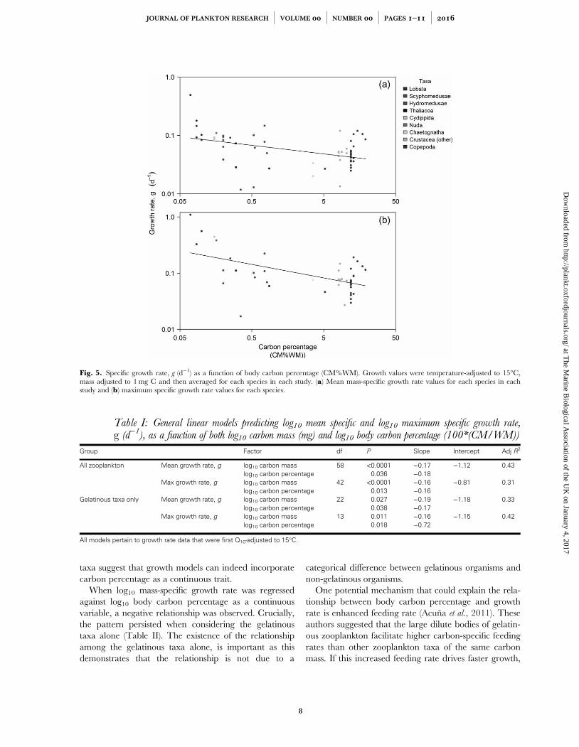
taxa suggest that growth models can indeed incorporatecarbon percentage as a continuous trait.
When log10 mass-specific growth rate was regressedagainst log10 body carbon percentage as a continuousvariable, a negative relationship was observed. Crucially,the pattern persisted when considering the gelatinoustaxa alone (Table II). The existence of the relationshipamong the gelatinous taxa alone, is important as thisdemonstrates that the relationship is not due to a
categorical difference between gelatinous organisms andnon-gelatinous organisms.One potential mechanism that could explain the rela-
tionship between body carbon percentage and growthrate is enhanced feeding rate (Acuña et al., 2011). Theseauthors suggested that the large dilute bodies of gelatin-ous zooplankton facilitate higher carbon-specific feedingrates than other zooplankton taxa of the same carbonmass. If this increased feeding rate drives faster growth,
Fig. 5. Specific growth rate, g (d−1) as a function of body carbon percentage (CM%WM). Growth values were temperature-adjusted to 15°C,mass adjusted to 1 mg C and then averaged for each species in each study. (a) Mean mass-specific growth rate values for each species in eachstudy and (b) maximum specific growth rate values for each species.
Table I: General linear models predicting log10 mean specific and log10 maximum specific growth rate,g (d−1), as a function of both log10 carbon mass (mg) and log10 body carbon percentage (100*(CM/WM))
Group Factor df P Slope Intercept Adj R2
All zooplankton Mean growth rate, g log10 carbon mass 58 <0.0001 −0.17 −1.12 0.43log10 carbon percentage 0.036 −0.18
Max growth rate, g log10 carbon mass 42 <0.0001 −0.16 −0.81 0.31log10 carbon percentage 0.013 −0.16
Gelatinous taxa only Mean growth rate, g log10 carbon mass 22 0.027 −0.19 −1.18 0.33log10 carbon percentage 0.038 −0.17
Max growth rate, g log10 carbon mass 13 0.011 −0.16 −1.15 0.42log10 carbon percentage 0.018 −0.72
All models pertain to growth rate data that were first Q10-adjusted to 15°C.
JOURNAL OF PLANKTON RESEARCH j VOLUME j NUMBER j PAGES – j at T
he Marine B
iological Association of the U
K on January 4, 2017
http://plankt.oxfordjournals.org/D
ownloaded from
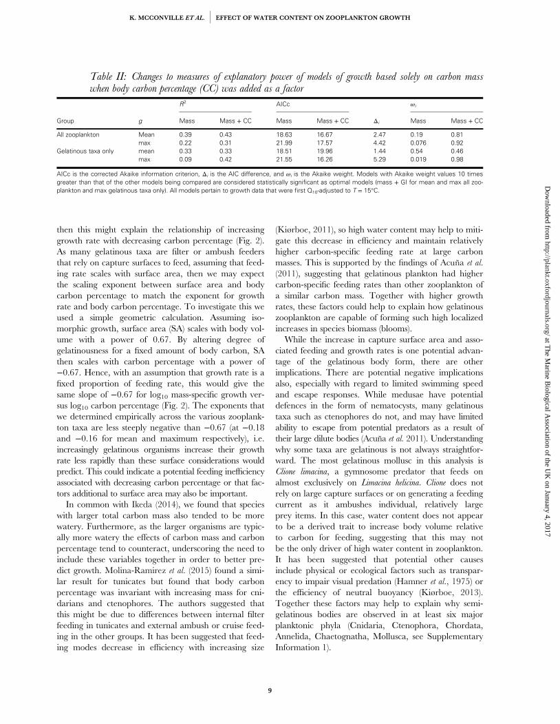
then this might explain the relationship of increasinggrowth rate with decreasing carbon percentage (Fig. 2).As many gelatinous taxa are filter or ambush feedersthat rely on capture surfaces to feed, assuming that feed-ing rate scales with surface area, then we may expectthe scaling exponent between surface area and bodycarbon percentage to match the exponent for growthrate and body carbon percentage. To investigate this weused a simple geometric calculation. Assuming iso-morphic growth, surface area (SA) scales with body vol-ume with a power of 0.67. By altering degree ofgelatinousness for a fixed amount of body carbon, SAthen scales with carbon percentage with a power of−0.67. Hence, with an assumption that growth rate is afixed proportion of feeding rate, this would give thesame slope of −0.67 for log10 mass-specific growth ver-sus log10 carbon percentage (Fig. 2). The exponents thatwe determined empirically across the various zooplank-ton taxa are less steeply negative than −0.67 (at −0.18and −0.16 for mean and maximum respectively), i.e.increasingly gelatinous organisms increase their growthrate less rapidly than these surface considerations wouldpredict. This could indicate a potential feeding inefficiencyassociated with decreasing carbon percentage or that fac-tors additional to surface area may also be important.In common with Ikeda (2014), we found that species
with larger total carbon mass also tended to be morewatery. Furthermore, as the larger organisms are typic-ally more watery the effects of carbon mass and carbonpercentage tend to counteract, underscoring the need toinclude these variables together in order to better pre-dict growth. Molina-Ramirez et al. (2015) found a simi-lar result for tunicates but found that body carbonpercentage was invariant with increasing mass for cni-darians and ctenophores. The authors suggested thatthis might be due to differences between internal filterfeeding in tunicates and external ambush or cruise feed-ing in the other groups. It has been suggested that feed-ing modes decrease in efficiency with increasing size
(Kiørboe, 2011), so high water content may help to miti-gate this decrease in efficiency and maintain relativelyhigher carbon-specific feeding rate at large carbonmasses. This is supported by the findings of Acuña et al.
(2011), suggesting that gelatinous plankton had highercarbon-specific feeding rates than other zooplankton ofa similar carbon mass. Together with higher growthrates, these factors could help to explain how gelatinouszooplankton are capable of forming such high localizedincreases in species biomass (blooms).
While the increase in capture surface area and asso-ciated feeding and growth rates is one potential advan-tage of the gelatinous body form, there are otherimplications. There are potential negative implicationsalso, especially with regard to limited swimming speedand escape responses. While medusae have potentialdefences in the form of nematocysts, many gelatinoustaxa such as ctenophores do not, and may have limitedability to escape from potential predators as a result oftheir large dilute bodies (Acuña et al. 2011). Understandingwhy some taxa are gelatinous is not always straightfor-ward. The most gelatinous mollusc in this analysis isClione limacina, a gymnosome predator that feeds onalmost exclusively on Limacina helicina. Clione does notrely on large capture surfaces or on generating a feedingcurrent as it ambushes individual, relatively largeprey items. In this case, water content does not appearto be a derived trait to increase body volume relativeto carbon for feeding, suggesting that this may notbe the only driver of high water content in zooplankton.It has been suggested that potential other causesinclude physical or ecological factors such as transpar-ency to impair visual predation (Hamner et al., 1975) orthe efficiency of neutral buoyancy (Kiørboe, 2013).Together these factors may help to explain why semi-gelatinous bodies are observed in at least six majorplanktonic phyla (Cnidaria, Ctenophora, Chordata,Annelida, Chaetognatha, Mollusca, see SupplementaryInformation 1).
Table II: Changes to measures of explanatory power of models of growth based solely on carbon masswhen body carbon percentage (CC) was added as a factor
Group g
R2 AICc
Δi
ωi
Mass Mass + CC Mass Mass + CC Mass Mass + CC
All zooplankton Mean 0.39 0.43 18.63 16.67 2.47 0.19 0.81max 0.22 0.31 21.99 17.57 4.42 0.076 0.92
Gelatinous taxa only mean 0.33 0.33 18.51 19.96 1.44 0.54 0.46max 0.09 0.42 21.55 16.26 5.29 0.019 0.98
AICc is the corrected Akaike information criterion, Δi is the AIC difference, and ωi is the Akaike weight. Models with Akaike weight values 10 timesgreater than that of the other models being compared are considered statistically significant as optimal models (mass + GI for mean and max all zoo-plankton and max gelatinous taxa only). All models pertain to growth data that were first Q10-adjusted to T = 15°C.
K. MCCONVILLE ET AL. j EFFECT OF WATER CONTENT ON ZOOPLANKTON GROWTH at T
he Marine B
iological Association of the U
K on January 4, 2017
http://plankt.oxfordjournals.org/D
ownloaded from
CONCLUSIONS
Body size is often described as a master-trait, and is fre-quently used as the sole intrinsic variable in empiricaland simulation models involving zooplankton growth(Kiørboe and Hirst, 2014; Andersen et al., 2015a). Butwhat do we mean by ‘body size’? Carbon mass is oftenused as the unit for size, but both our meta-analysis andthe real assemblage data show that carbon percentagealso varies greatly. It may even vary negatively with car-bon mass, levering an opposing effect on growth. Weargue that carbon mass and carbon percentage are bothkey traits, both are intrinsic to the zooplankton andsince they are possible to estimate, then we should disen-tangle their separate effects in a unified growth model.By including carbon percentage in models of growthbased on carbon mass alone, we substantially increasedtheir explanatory power, with smaller body masses andlower body carbon percentages leading to higher specificgrowth rates. Building on the work of previous publica-tions (Kiørboe, 2013; Pitt et al., 2013; Molina-Ramirezet al., 2015) we provide a carbon percentage dataset inSupplementary Table 1. By using these source data along-side carbon mass, the maximum growth rate equation inTable 1 may then be used as a starting point to estimategrowth rates attainable by zooplankton.
Alongside the ‘size’ based simplifications used formodelling, there has also been an increase in ‘trait-based’ modelling in which categorical variables orfunctional groups are allowed to vary continuously. Apurpose of this article is to allow water content also tobe used as a continuous trait; to facilitate its inclusionalongside carbon mass and other traits such as feedingmode (Litchman et al., 2013; Andersen et al. 2015a;Hérbert et al., 2016). Since we found that growth ratedepended on carbon percentage even among the gelat-inous taxa alone, we hope that considering and model-ling water content as a continuous trait will reveal theecological and evolutionary factors that influence thewater content of zooplankton.
SUPPLEMENTARY DATA
Supplementary data can be found online atPlankton Research journal.
ACKNOWLEDGEMENTS
We thank the numerous authors (cited inSupplementary Tables 1 and 2) whose measurements ofbody composition and growth rate have made this
meta-analysis possible. We also thank the crew of theRV Plymouth Quest and Anderson Rachel Harmer andAndrea McEvoy who analysed the zooplankton data.We thank Martin Lilley for help with the length-massconversions of the gelatinuous taxa.
FUNDING
K.M. was in receipt of a Natural Environment ResearchCouncil National (NERC) funded studentship, and waspartly funded together with A.A., E.F. and A.G.H. bythe NERC and Department for Environment, Food andRural Affairs (Grant no. NE/L003279/1, MarineEcosystems Research Program).
REFERENCESAcuña, J.L. (2001) Pelagic tunicates: why gelatinous? Am. Nat., 158,100–106.
Acuña, J.L., López-Urrutia, A. and Colin, S. (2011) Faking giants: theevolution of high prey clearance rates in jellyfishes. Science, 333,1627–1629.
Andersen, K.H, Aksnes, D.L., Berge, T., Fiksen, Ø. and Visser, A.(2015a) Modelling emergent trophic strategies in plankton.J. Plankton Res., 37, 862–868.
Andersen, K.H., Berge, T., Goncalves, R.J., Hartvig, M., Heuschele,J., Hylander, S., Jacobsen, N.S., Lindemann, C. et al. (2015b)Characteristic sizes of life in the oceans, from bacteria to whales.Annu. Rev. Mar. Sci., 8, 3.1–3.25 2016.
Atkinson, A., Harmer, R.A., Widdicombe, C.E., McEvoy, A.J.,Smyth, T.J., Cummings, D.G., Somerfield, P.J., Maud, J.L. et al.(2015) Questioning the role of phenology shifts and trophic mis-matching in a planktonic food web. Prog. Oceanogr., 137, 498–512.
Bone, Q. (1998) The Biology of Pelagic Tunicates. Oxford University Press,Oxford.
Brown, J.H., Gillooly, J.F., Allen, A.P., Savage, V.M. and West, G.B.(2004) Toward a metabolic theory of ecology. Ecology, 85,1771–1789.
Burnham, K. P. and Anderson, D. R. (2002) Model Selection and
Multimodel Inference: A Practical Information-Theoretic Approach. Springer,New York.
Clarke, A., Holmes, L.J. and Gore, D. J. (1992) Proximate and elem-ental composition of gelatinous zooplankton from the SouthernOcean. J. Exp. Mar. Biol. Ecol., 155, 55–68.
Condon, R.H, Duarte, C.M., Pitt, K.A., Robinson, K.L., Lucas, C.H.,Sutherland, K.R., Mianzan, H.W., Bogeberg, M. et al. (2013)Recurrent jellyfish blooms are a consequence of global oscillations.Proc. Natl. Acad. Sci. U.S.A., 110, 1000–1005.
Belsley, D., Kuh, E. and Welsch, R. (1980) Regression Diagnostics.Wiley, Hoboken, New Jersey, USA.
Eloire, D., Somerfield, P.J., Conway, D.V.P., Halsband-Lenk, C.,Harris, R. and Bonnet, D. (2010) Temporal variability and commu-nity composition of zooplankton at station L4 in the WesternChannel: 20 years of sampling. J. Plankton Res., 32, 657–679.
JOURNAL OF PLANKTON RESEARCH j VOLUME j NUMBER j PAGES – j at T
he Marine B
iological Association of the U
K on January 4, 2017
http://plankt.oxfordjournals.org/D
ownloaded from
Gemmell, B.J., Costello, J.H., Colin, S.P., Stewart, C.J., Dabiri, J.O.,Tafti, D. and Priya, S. (2013) Passive energy recapture in jellyfishcontributes to propulsive advantage over other metazoans. Proc.
Natl. Acad. Sci. U.S.A., 110, 17904–17909.
Gibbons, M.J. and Richardson, A.J. (2013) Beyond the jellyfish joyrideand global oscillations: advancing jellyfish research. J. Plankton Res.,35, 929–938.
Gillooly, J.F., Brown, J.H., West, G.B., Savage, V.M. andCharnov, E.L. (2002) Effects of size and temperature on metabolicrate. Science, 293, 2248–2251.
Hamner, W.M., Madin, L.P., Alldredge, A.L., Gilmer, R.W. andHamner, P.P. (1975) Underwater observations of gelatinous zoo-plankton: Sampling problems, feeding biology, and behavior.Limnol. Oceangr., 20, 907–917.
Hansen, P.J., Bjørnsen, P. K. and Hansen, B.W. (1997) Zooplanktongrazing and growth: scaling within the 2–2000 μm body size range.Limnol. Oceanogr., 42, 687–704.
Harbison, G.R. (1992) The gelatinous inhabitants of the ocean inter-ior. Oceanus, 35, 18–23.
Harris, R. (2010) The L4 time series: the first 20 years. J. Plankton Res.,32, 577–583.
Hendrickx, J. (2012). Perturb: Tools for Evaluating Collinearity. R packageversion 2.05. http://CRAN.R-project.org/package=perturb
Hérbert, M-P., Beisner, B.E. and Maranger, R. (2016) Linking zoo-plankton communities to ecosystem functioning: toward an effect-trait framework. J. Plankton Res., 00, 1–10.
Hirst, A.G. (2012) Intra-specific scaling of mass to length in pelagicanimals: ontogenetic shape change and its implications. Limnol.
Oceanogr., 57, 1579–1590.
Hirst, A.G. and Forster, J. (2013) When growth models are not univer-sal: evidence from marine invertebrates. Proc. R. Soc. B, 280,20131546, http://dx.doi.org/10.1098/rspb.2013.1546.
Hirst, A.G., Roff, J.C. and Lampitt, R.S. (2003) A synthesis of growthrates in marine epipelagic invertebrate zooplankton. Adv. Mar. Biol.,44, 1–142.
Ikeda, T. (2014) Synthesis toward a global model of metabolism andchemical composition of medusae and ctenophores. J. Exp. Mar.
Biol. Ecol., 456, 50–64.
Kiørboe, T. (2011) How zooplankton feed: mechanisms, traits andtrade-offs. Biol. Rev., 86, 311–339.
Kiørboe, T. (2013) Zooplankton body composition. Limnol. Oceanogr.,58, 1843–1850.
Kiørboe, T. and Hirst, A.G. (2014) Shifts in mass scaling of respir-ation, feeding, and growth rates across life-form transitions in mar-ine pelagic organisms. Am. Nat., 183, 118–130.
Litchman, E., Ohman, M.D. and Kiørboe, T. (2013) Trait-basedapproaches to zooplankton communities. J. Plankton Res., 35,473–484.
Lucas, C.H., Pitt, K.A., Purcell, J.E., Lebrato, M. and Condon, R.H.(2011) What’s in a jellyfish? Proximate and elemental compositionand biometric relationships for use in biogeochemical studies.Ecology, 92, 1704–1704.
Maud, J.L., Atkinson, A., Hirst, A.G., Lindeque, P.K., Widdicombe,C.E., Harmer, R.A., McEvoy, A. and Cummings, D.G. (2015) Howdoes Calanus helgolandicus maintain its population in a changing cli-mate? Analysis of a 25-year time series from the English Channel.Prog. Oceanogr., 137, 513–523.
Molina-Ramirez, A., Caceres, C., Romero-Romero, S., Bueno, J.,Ignacio Gonzalez-Gordillo, J., Irigoien, X., Sostres, J., Bode, A.et al. (2015) Functional differences in the allometry of the water, car-bon and nitrogen content of gelatinous organisms. J. Plankton Res.,35, 989–1000.
Møller, L.F. and Riisgård, H.U. (2007) Feeding, bioenergetics andgrowth in the common jellyfish Aurelia aurita and two hydromedu-sae, Sarsia tubulosa and Aequorea vitrina. Mar. Ecol. Prog. Ser., 346,167–177.
Peters, R.H. (1983) The Ecological Implications of Body Size. CambridgeUniversity Press, Cambridge.
Pitt, K.A., Duarte, C.M., Lucas, C.H., Sutherland, K.R., Condon, R.H., Mianzan, H., Purcell, J.E., Robinson, K.L. et al. (2013) Jellyfishbody plans provide allometric advantages beyond low carbon per-centage. PLoS One, 8, e72683.
Pond, D.W., Harris, R.P., Head, R.N. and Harbour, D. (1996)Environmental and nutritional factors determining seasonal variabil-ity in the fecundity and egg viability of Calanus helgolandicus in coastalwaters off Plymouth, U.K.. Mar. Ecol. Prog. Ser., 143, 45–63.
Purcell, J.E. (2012) Jellyfish and Ctenophora blooms coincide withhuman proliferations and environmental perturbations. Annu. Rev.Mar. Sci, 4, 209–235.
R Core Team. (2014) R: A Language and Environment for Statistical
Computing. R Foundation for Statistical Computing, Vienna, Austria.http://www.R-project.org/.
Richardson, A.J., Bakun, A., Hays, G.C. and Gibbons, M.J. (2009)The jellyfish joyride: causes, consequences and managementresponses to a more gelatinous future. Trends Ecol. Evol., 24,312–322.
Royall, R.M. (1997) Statistical Evidence: A Likelihood Paradigm. Chapmanand Hall, New York, NY.
Shiganova, T.A. and Bulgakova, Y.V. (2000) Effects of gelatinousplankton on Black Sea and Sea of Azov fish and their foodresources. ICES J. Mar. Sci., 57, 641–648.
Smyth, T., Atkinson, A., Widdicombe, S., Frost, M., Allen, I.,Fishwick, J., Quieros, A., Sims, D. and Barange, M. (2015) TheWestern Channel. Prog. Oceanogr., 137, 335–341.
Sutherland, K.L., Madin, L.P. and Stocker, R. (2010) Filtration of sub-micrometer particles by pelagic tunicates. Proc. Nat. Acad. Sci. U.S.A.,107, 15129–15134.
K. MCCONVILLE ET AL. j EFFECT OF WATER CONTENT ON ZOOPLANKTON GROWTH at T
he Marine B
iological Association of the U
K on January 4, 2017
http://plankt.oxfordjournals.org/D
ownloaded from