do recessions affect environmental concern and …deryugina.com/2014-10-17_draft.pdf · do...

1

Do Recessions Affect Environmental Concern and Does it Matter for Real Outcomes?*

Tatyana Deryugina+ and Xian Liu++

October 2014

Abstract:

A unique feature of the environment is that the consequences of its use are often difficult or

impossible to reverse. This implies that short-run changes in environmental policies brought

about by preference changes can result in long-run effects. We estimate how environmental

attitudes change with economic conditions and whether these changes affect voting behavior

or the actions of elected representatives. We show that, even though attitudes toward the

environment are strongly influenced by local economic conditions, as measured by income and

the unemployment rate, they do not immediately translate into changes in real outcomes. This

is consistent with individuals being “issue voters”, with the environment being a relatively low-

priority issue.

* We thank Nolan Miller and Julian Reif for helpful discussions. + Department of Finance, University of Illinois at Urbana-Champaign, 1206 South Sixth St., Champaign, IL, USA. e-mail: [email protected]. ++ Department of Economics, Tulane University. e-mail: [email protected].

2

I. Introduction

Environmental quality, such as clean air and clean water, is thought to be a normal good:

as incomes increase, so does the relative demand for environmental quality. By making the

average individual poorer and possibly by lowering expectations about future income,

recessions should then lower the demand for environmental quality. If such changes in demand

are accompanied by a weakening of environmental policy, recessions may cause permanent

environmental damage.

We estimate how environmental concerns change with economic conditions, using a

nationally representative survey that spans eleven years and directly elicits individuals’

tradeoffs between economic growth and environmental quality. We use state-level

unemployment rates and county-level incomes as proxies for local economic conditions. We

find strong evidence that willingness to sacrifice economic growth for environmental protection

decreases with a state’s unemployment rate and increases with a county’s income. In our

preferred specification, which includes state and year fixed effects, a 1% increase in the state’s

unemployment rate decreases the probability that the respondent chooses environmental

protection over economic growth by 0.21-0.67%. Similarly, a 1% fall in the per capita income in

the county decreases the probability that the respondent chooses to prioritize the environment

over the economy by about 0.11-0.12%.

We then tackle the question of whether these changes in beliefs translate into real

policy effects, either through how individuals vote for their representatives or how their

representatives vote in Congress. Because the Democratic Party is traditionally thought to be

more concerned about the environment, we first consider whether voters are more likely to

vote for Republicans when their concern for the environment declines. We find no evidence for

this hypothesis, although it is possible that our estimates are affected by measurement error.

We then test whether representatives adapt to their constituents’ changing views by

estimating how the voting patterns of representatives change following a change in

constituents’ views. We find that there is no change in how representatives vote, as measured

by a party unity score, an economic ideology score, or an environmental friendliness score.

3

Thus, although changes in economic conditions affect beliefs, the beliefs in turn do not affect

voting patterns of the citizens themselves or of their representatives, at least in the short run.

Our results are consistent with the idea that people are “issue voters” (Margolis, 1977;

Rabinowitz and Macdonald, 1989). That is, instead of basing her voting decisions on a

politician’s entire policy platform, a voter will focus on the politician’s positions on just a few

aspects of public policy that are important to her (e.g., taxes or gun control). The environment

appears to be a low-salience issue in politics (Guber, 2001; Repetto, 2006). Relatedly, in a 2011

Gallup survey, environmental degradation was rated as the most important problem facing the

nation by only 1% of respondents, and ranked 22nd overall. In this case, even large relative

changes in environmental concern may not translate into meaningful changes in voting.

To our knowledge, there is only one paper examining the role of economic conditions on

environmental preferences at the sub-national level (Kahn and Kotchen, 2011). We build on

their work by using nationwide data and by considering voting and policy outcomes as well. We

also contribute to the broad literature on the drivers of environmental preferences (e.g., Jones

and Dunlap, 1992; Greely, 1993; Jones and Carter, 1994; Blocker and Eckberg, 1997; Elliott et al.,

1997; Kanagy, Humphrey, and Firebaugh, 1994; Klineberg, McKeever, and Rothenbach, 1998;

Uyeki and Holland, 2000). Unlike these previous studies, however, our results are unlikely to be

contaminated by endogeneity or simultaneity.

The rest of this paper is organized as follows. Section II describes how changes in

economic conditions can result in changes in environmental attitudes and actual behavior.

Section III describes our data. Section IV outlines the empirical framework and identification

assumptions. Section V presents and discusses the results. Section VI concludes.

II. Conceptual framework Preferences

Suppose that individuals have preferences over environmental quality and other

consumption goods and that their preferences can be represented by a single utility function

𝑈(𝐸,𝑋), where 𝐸 is environmental quality and 𝑋 is all other consumption goods. Incomes are

given by 𝐼 = 𝐽 ∗ 𝑊 + (1 − 𝐽) ∗ 𝑇, where 𝐽 is an indicator equal to 1 if the individual is working

4

and 0 otherwise, and 𝑊 and 𝑇 are the earnings the individual receives when working and not

working, respectively. The variable 𝑇 can be thought of as unemployment insurance payments

and we thus assume that 𝑇 < 𝑊. Average aggregate income will be equal to 𝐼 ̅ = (1 − 𝑈) ∗

𝑊 + 𝑈 ∗ 𝑇, where 𝑈 is the aggregate unemployment rate.

If the average wage falls or the aggregate unemployment rate rises, the average aggregate

income will fall. If environmental quality is a normal good, as is commonly assumed, individuals

will want to consume less of it and will be willing to trade off a decrease in 𝐸 for a decrease in 𝑈

or increase in 𝑊.1 However, because environmental quality is typically a public good (e.g., clean

air and water), we will not necessarily observe a decrease in consumption. Instead, one result

may be that individuals will state that they prefer a lower environmental quality and higher

economic growth.

Many studies have shown that economic factors, especially macroeconomic conditions and

economic expectation, appear to play an important role in shaping general attitudes toward

public policy. Vogel (1989) finds that public attitudes toward regulation are dramatically driven

by changing economic conditions. For example, during good economic times people are more

supportive of implementing stringent regulatory efforts on business. Durr (1993) shows that

public opinion about domestic policy responds strongly to changes in economic expectations.

Specifically, expectations of a strong economy result in greater support for liberal domestic

policies, while expectations of declining economic circumstances generate more conservative

sentiment.

There is also empirical evidence that macroeconomic conditions are correlated with public

environmental attitudes specifically. Elliott et al. (1995) and Johnson et al. (2005) find that, as

real income increases, the public in the US are more supportive of increasing expenditure on

environmental protection. This relationship between economic prosperity and environmental

concern has also been found in many other countries (Inglehart, 1995). However, much of this

work has been cross-sectional or used time series data, making it more likely that other

confounding factors may have been present.

1 Individuals may also be altruistic toward others. In this case, we would expect the subsequent changes in attitudes or voting behaviors to be more pronounced.

5

Citizens’ voting behavior

Observed changes in preferences may translate into changes in voting behavior. Work in

political science and political economy has developed several models of voter and

representative behavior that can be used to make predictions about the effect of changes in

attitudes on voters and representatives. If voter preferences change, so can the share of votes

going to a particular party.

Because environmental protection is typically thought of as a normal good, we expect to

see higher unemployment rates and lower income increasing the likelihood that individuals

prefer to sacrifice environmental protection for economic growth. This, in turn, should make

some of them more likely to vote for candidates that will promote economic growth over

environmental protection. Because the Democratic Party has traditionally been more likely to

promote environmental protection legislation, the party affiliation of a candidate may be a

good proxy for the likelihood that he or she will choose economic growth over environmental

protection.

However, predicting how changes in preferences translate into changes in voting behavior is

not straightforward. If environmental concerns are secondary to voters, then even a large

change in environmental preferences will not necessarily alter how they vote. Previous

literature has found that people tend to base their votes on a few issues that are important to

them rather than all possible issues. Thus, even if their opinions about some issues change,

their voting patterns may not.

Only a handful of studies examine the relationship between environmental concern and

voting behavior, and they find mixed results. Some studies find that environmental concerns

seldom shape individual vote preference because of low salience (Ladd and Bowman, 1995;

Repetto, 2006). Guber (2001) finds that preferences for protecting the environment over jobs

have little impact on electoral choice in the 1996 presidential election. However, other studies

find that environmental opinions influence constituents’ voting choices. For instance, Davis and

Wurth (2003) find that the attitude towards federal spending on environmental protection is a

significant predictor of voters’ candidate choice in the 1996 presidential election. Davis et al.

(2008) also find that attitudes towards federal spending on the environment had a significant

6

impact on presidential vote in 1984, 1988, 1992 and 1996. Voters more supportive of increasing

spending on environmental protection were more likely to vote for Democratic candidates.

Overall, whether changes in environmental attitudes affect people’s voting behavior is an

empirical question.

If we find that, following changes in environmental preferences, voting behavior does not

change, there are two possible interpretations. One is that the environment is a low-priority

issue for most voters, as discussed above. However, a second interpretation is that politicians

countered the changes in voting patterns by changing their own behavior, a possibility that we

explore below.

Representatives’ voting behavior

Politicians can pre-empt changes in voters’ behavior by changing their platform or

legislative behavior to reflect the voters’ preferences. The overall evidence for whether

politicians respond meaningfully to electoral incentives is mixed. For example, List and Sturm

(2006) and Fredriksson et al. (2011) find that electoral incentives are significant determinants of

environmental policy at the state level. Conversely, Lee et al. (2004) find that general policy

choices of legislators in the US House of Representatives are unrelated to the margin with

which they are elected, suggesting that voter preferences have little effect on behavior.

Political scientists have long believed that public opinion has a significant impact on public

policy agenda in democratic countries.2 In their seminal work, Page and Shapiro (1983) present

evidence that public opinion changes are important causes of policy change in the US politics,

especially for highly salient issues. Erikson et al. (1993) examine the linkages between public

political attitudes and the choice of state-level policy makers, and find that states with more

liberal publics tend to pass more liberal policies across a wide range of policy domains.

Extending this work, Brace et al. (2002) and Norrander (2001) find that specific public attitudes

influence specific state policy outcomes, even after controlling for the impact of public ideology.

Stimson (1991) and Stimson et al. (1995) find that members of the Congress translate changes

2 Burstein (2003) provides a good review of the impact of public opinion on public policy.

7

in public opinion into policy change: when electoral politicians sense a shift in public

preferences, they act accordingly to shift the direction of public policy.

A few studies have also examined the impact of environmental opinion on public policy.

Brace et al. (2002) have demonstrated that public opinions about environmental spending have

significant impacts on state-level environmental policy implementation. Hays et al. (1996) find

that states with more liberal publics tend to elect liberal officials who in turn propose more

stringent state-level environmental regulations.

There are three important reasons for why changes in voters’ attitudes may not lead to

changes in their representatives’ behavior. First, changes in environmental attitudes may not

translate into changes in voting behavior, as discussed in the previous section. Second,

politicians may be catering to voters who are located in a particular place on the voter

preference spectrum (e.g., Downs, 1957): if the voting behavior of those marginal voters does

not change, neither will the behavior of politicians. Third, politicians may not be able to commit

to implement the promised policies once in office, putting in place their preferred policies

instead (e.g., Lee et al., 2004). Thus, whether changes in preferences translate into policy

changes is an empirical question that we test below.

III. Data Description and Summary Statistics

Our public opinion dataset is Gallup’s annual Environmental Poll for the years 2000-

2011. In March of each year, Gallup conducts a nationally representative telephone poll of

about 1,000 adults to gauge their attitudes toward economic, environmental, and political

issues.3 For the years 2000-2002, only the respondent’s state of residence is available, while the

later years also contain the county of residence.

Our primary goal is to estimate the relationship between economic conditions, proxied

for by the prevailing unemployment rate or mean income, and whether respondents prioritize

environmental protection over economic growth. A key advantage of our dataset is that it

contains a question aimed at capturing this exact tradeoff. Specifically, respondents are asked

3 The annual surveys each contain about 30 questions. Respondents are randomly chosen and interviewed by both landline telephones and cellular phones. More details about the survey mechanism can be found from Gallup’s Environment Poll Survey at http://www.gallup.com/tag/Environment.aspx.

8

to choose whether they most agree that “protection of the environment should be given

priority, even at the risk of curbing economic growth” or that “economic growth should be

given priority, even if the environment suffers to some extent.” In our empirical analysis, we

code respondents who choose to prioritize environmental protection as 1 and respondents who

choose to prioritize economic growth as 0.

Our first proxy for the prevailing economic conditions is the average unemployment rate

in the respondent’s state over the past 12 months prior to taking the survey. We use monthly,

seasonally adjusted state-level unemployment rates, as reported by the Bureau of Labor

Statistics.4

Our second proxy is the average per-capita income in a county, which we obtain from

the Regional Economic Information Systems (REIS). Several measures are available: we use the

per-capita net earnings by residents (hereafter referred to as “per-capita income”). Because the

surveys are always conducted in March, we use the previous year’s mean income as the

independent variable.

Our voting data comes from Dave Leip’s “Atlas of US Presidential Elections.” We have

county-level voting data for the 2000, 2004, and 2008 presidential elections, as well as for each

House and Senate election between 2000 and 2010. The datasets contain the number of votes

cast for the Democratic and Republican parties in each election. From this, we construct a

measure of the percent of voters who vote for the Democratic Party.

Because a change in voter priorities can affect the behavior of congressmen with

respect to the environment, the economy, or both, we use several proxies to capture changes

in congressmen’s behavior. Our first proxy is Poole and Rosenthal’s DW-Nominate score for

each member of Congress (Poole and Rosenthal, 1997).5 The DW-Nominate score estimates the

ideological position of each representative using roll call voting records taken in each

Congress.6 It has two dimensions: the first measures ideology on economic matters, while the

second measures attitudes about salient social issues of the particular period for which it is

4 County-level unemployment rates are also available for a subset of the counties in our sample. However, because using county-level rates drastically reduces our sample, we do not use them. 5 Available from voteview.com. 6 The scores are calculated using a three-step estimation procedure in which each legislator is assumed to make voting choices that maximize his utility function (Poole and Rosenthal, 1997).

9

calculated. Because the second dimension is unlikely to be useful in our setting, we focus on the

first. The score for the first dimension ranges from -1 (most liberal) to 1 (most conservative).

During our study period, the average DW-Nominate score for Republican members is 0.61, and

that for Democratic members is -0.37 (see Table A1). To arrive at our final measure of economic

ideology, we average each state’s representatives’ scores in each year.

Our second proxy for representatives’ behavior is Poole and Rosenthal’s party unity

scores for each legislator, also computed from roll call voting records. It is defined as the

percentage of “party unity votes” in which the member voted with his party’s majority.7 Thus, a

higher value of the party unity score indicates that the legislator is more likely to vote along

with the majority of his party. As Table A1 shows, the average party unity scores for the two

parties are quite close, but Republican members have a smaller variance. If a legislator’s

constituents become more willing to sacrifice economic growth for the environment, we may

expect Democrats to become more willing to vote with their party (i.e., party unity increases)

while Republicans should become less willing to vote with their party (i.e., party unity

decreases). Thus, we average the party unity scores by state and year separately for

Republicans and Democrats.

Finally, to capture behavior directly related to the environment, we use the National

Environmental Scorecard produced by the League of Conservation Voters (LCV).8 LCV keeps

track of the most important pieces of environmental legislation each year and how

Congressmen vote on these. The annual LCV score is the percentage of pro-environment votes

cast by each representative, ranging from 0 to 100. Table A1 summarizes the LCV scores of

congressional representatives during out study period. The average score is 50.44; Democrats

score much higher than Republicans (a mean of 87 versus 13), supporting our assumption that

the Democratic Party is on average more pro-environment. We assume that all of these

measures remain constant throughout the two years of each Congressional session; thus, the

state-level measures change every two years.

7 A party unity vote is defined as one where at least 50% of one party votes in opposition to at least 50% of the other party. 8 Available from www.lcv.org. We do not need to adjust the LCV scores to account for structural changes over time (e.g., as in Shipan and Lowry, 1997); the presence of year fixed effects in our specifications accomplishes that in a fully non-parametric way.

http://www.lcv.org/

10

Table 1 shows the weighted summary statistics for our sample. Panel A shows the key

variables for the analysis. Of 11,012 respondents, 55% gave priority to the environment over

economic growth.9 The average state-level unemployment rate at the time the respondents

were surveyed was about 5.8% with a standard deviation of 2. Per capita income averaged

$26,000 in nominal terms, with a standard deviation of $8,500.

Panel B in Table 1 summarizes respondent characteristics. The mean respondent is

about 47 years old, about half of the respondents are male and the overwhelming majority

(84%) is white. Almost 35% of the sample is not in the labor force, which is explained by a large

fraction (20%) of retired respondents. About 40% of the respondents consider themselves

conservative or very conservative while about 20% consider themselves liberal or very liberal.

Finally, about 40% of our sample has at most a high school degree.

[TABLE 1 ABOUT HERE]

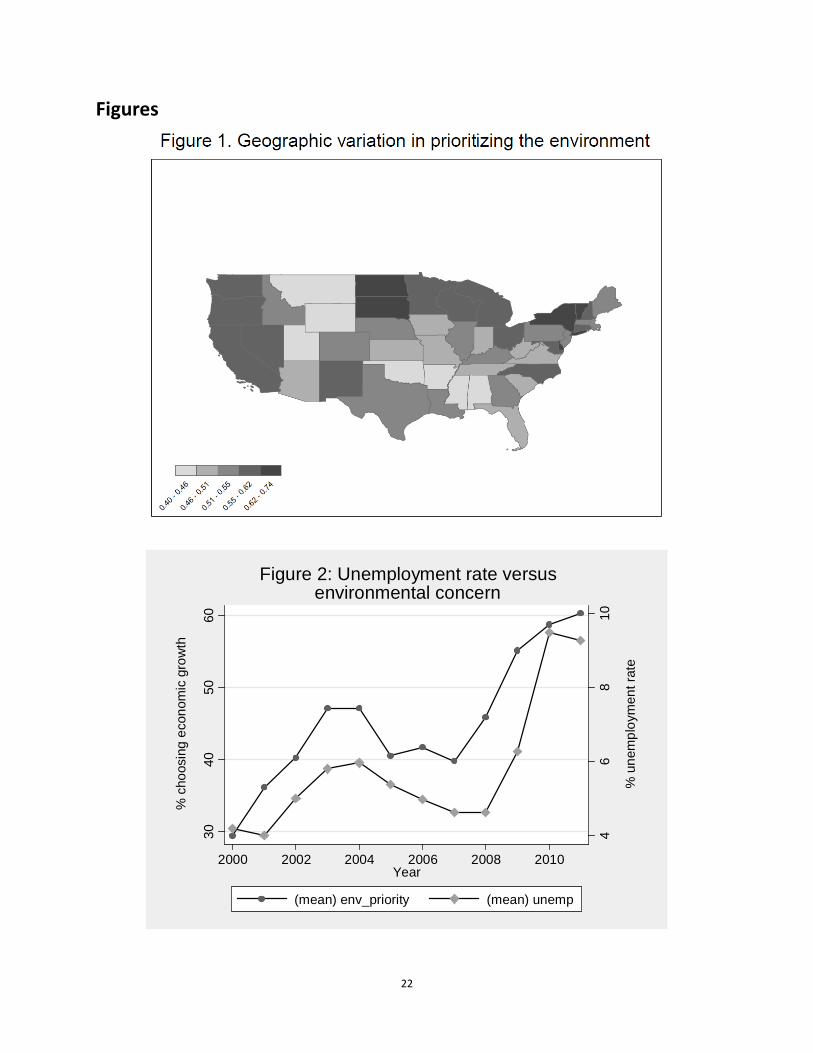
Figure 1 shows the geographic distribution of preferences over the whole time period,

with darker areas signifying a larger fraction of respondents preferring environmental

protection to economic growth. There is no significant geographic concentration of preferences,

although states like California, Washington and Oregon score predictably high.

[FIGURE 1 ABOUT HERE]

Figure 2 presents the national trends for unemployment and environmental concern for

2000-2011.10 For expositional purposes, we show the environmental concern variable as the

percentage of respondents choosing economic growth over environmental protection. Both

measures decrease steadily after 2003 and increase rapidly starting in late 2007, suggesting a

strong association between the two at the national level. Notably, from 2007 to 2010, the

9A very small portion of respondents answered that environmental protection and economic growth are equally important, although this was not one of the formal answer choices. We drop these observations along with respondents who answered “don’t know” or refused to answer the question. 10 Figures 2 and 3 use sampling weights to make the graphs representative of the entire U.S. population.

11

average state level unemployment rate increased substantially from about 4.5% to over 9.5%,

while the share of respondents choosing economic growth over the environment increased

from about 35% to nearly 60%.


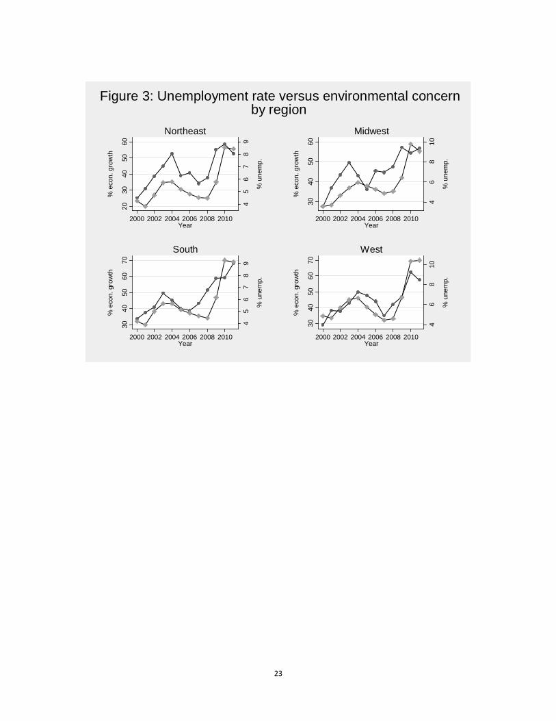
Figure 3 plots the trends separately for each of the four US regions: Northeast, Midwest,

South and West. A pattern similar to that in Figure 1 emerges: both measures decrease after

2003 and increase substantially after 2007. This graphic evidence supports the idea that there is

a strong positive relationship between economic conditions and environmental concern

throughout the US. Later in the paper, we investigate whether this relationship persists once

various controls are included.


IV.Empirical Strategy The effect of unemployment rates and income on prioritizing the environment

To estimate the effect of statewide unemployment rates on public opinion, we use the

following regression model:

𝐸𝐸𝐸𝐸𝐸𝐸𝐸𝐸𝐸𝐸𝐸ist = 𝛽1Unemployments,t−1 + 𝑿𝒊′θ + αs + αt + εist (1)

where i indexes respondents, s indexes states, and t indexes years. The variable

𝐸𝐸𝐸𝐸𝐸𝐸𝐸𝐸𝐸𝐸𝐸𝑖𝑖𝑖 is an indicator equal to 1 if the respondent prefers to prioritize environmental

protection over economic growth and 0 otherwise. The variable 𝑈𝐸𝐸𝐸𝑈𝑈𝐸𝑈𝐸𝐸𝐸𝐸𝑖,𝑖−1 is the

average monthly unemployment rate in state s over the previous 12 months.11 We use this

measure because it is more likely to represent the underlying economic conditions than the

unemployment rate in any single month. We control for age, gender, race, educational level,

11Because all respondents were interviewed in March each year, the lagged unemployment rates are measured as the average unemployment rates from March of last year to February of this year for each state. For the sake of exposition, we use the subscript t-1 to represent this measure.

12

employment status, political ideology, and household income with the vector 𝑿𝒊. Finally, we

include state fixed effects, 𝛼𝑖, to account for time-invariant unobserved factors that vary across

states and year fixed effects, 𝛼𝑖, to control for temporal changes that are common to all states.

The coefficient of primary interest is 𝛽1, which reflects the relationship between

changes in the statewide unemployment rate and changes in the environmental concern of the

public. Identification of the model comes from variation in a state’s unemployment rate over

time relative to the rest of the country. A positive estimate indicates that an increase in the

unemployment rate leads to increased public support for prioritizing economic growth over the

environment.

Because our dependent variable is binary, we use a probit specification to estimate

Equation 1.12 We use survey sampling weights provided by Gallup to make the estimates

representative of the entire U.S population. Because the error terms are likely to be correlated

across time, all standard errors are clustered at the state level.

In addition to state-level employment rates, we use county-level measures of mean

income to validate our results:

𝐸𝐸𝐸𝐸𝐸𝐸𝐸𝐸𝐸𝐸𝐸ist = 𝛽2log (Incomec,t−1) + 𝑿𝒊′θ + αs + αt + εist (2)

where 𝐼𝐸𝐼𝐸𝐸𝐸𝑐,𝑖−1 is the average annual per capita net income by residents in county c in the

previous year. The coefficient 𝛽2 provides an estimate of how changes in county income levels

affect the public concern for the environment.

We interpret the relationship between environmental concern and unemployment

levels casually, where the latter affects the former. In order to be able to do so, it must be true

that there does not exist an unobservable factor driving both economic conditions and

environmental concern at the state-year level. While we cannot test for its presence, we cannot

think of a reasonable example where such a confounding factor exists.

Another requirement for causal interpretation is no reverse causality; in other words,

environmental concern cannot affect economic conditions. While one can think of extreme

12 We estimate a linear probability model as a robustness check. Results are very similar and can be found in the Appendix.

13

examples where this is violated (e.g., a boycott of environmentally damaging goods causing its

producer to go bankrupt thus raising the unemployment rate), we believe the lack of reverse

causality is a reasonable assumption in our context.

The effect of environmental concern on citizens’ and representatives’ voting behavior

We proceed to test whether changes in environmental concern in the county change

voting patterns, either of citizens or their representatives. First, we estimate whether the share

of individuals voting Republican decreases when people become relatively more concerned

about the environment:

𝑅𝐸𝑈𝑖𝑖 = 𝛾1𝐸𝐸𝐸𝐸𝐸𝐸𝐸𝐸𝐸𝐸𝐸𝑖𝑖 + 𝛼𝑖 + 𝛼𝑖 + 𝜀𝑐𝑖 (3)

where 𝑅𝐸𝑈𝑖𝑖 is the fraction of individuals voting Republican in either the House or Senate

election, and 𝐸𝐸𝐸𝐸𝐸𝐸𝐸𝐸𝐸𝐸𝐸𝑖𝑖 is the average of respondents’ environmental concern in state s

and year t. If there is a change in voting patterns, we expect 𝛾1 to be negative: in other words,

as the average person in the county becomes more likely to prefer environmental protection

over economic growth, she becomes less likely to vote Republican.

If there is any change in representatives’ voting patterns, we expect Congressmen in

both parties to become more likely to vote for environmental protection as their constituents’

preferences for it increase. We test whether changes in environmental concern change

Congressmen’s voting behavior with the following specification:

𝑉𝐸𝐸𝐸𝐸𝑉_𝑠𝐼𝐸𝐸𝐸𝑝𝑖𝑖 = 𝛾2𝐸𝐸𝐸𝐸𝐸𝐸𝐸𝐸𝐸𝐸𝐸𝑖𝑖 + 𝛼𝑖 + 𝛼𝑖 + 𝜀𝑖𝑖 (4)

where 𝑉𝐸𝐸𝐸𝐸𝑉_𝑠𝐼𝐸𝐸𝐸𝑝𝑖𝑖 is either the average party unity score or pro-environmental score of

all Congressmen from party 𝑈 and state 𝑠 in year 𝐸. The party is either Democrat or Republican.

Because the Democratic Party has traditionally been thought of as more likely to vote for

environmental protection, we expect Democrats to become more unified with their party

(𝛾2 > 0 when we look at Democrats), while Republicans should become less unified (𝛾2 < 0

when we look at Republicans). When the dependent variable is the pro-environmental score,

14

we expect representatives from both parties to receive higher scores when their constituents’

preferences for environmental protection increase (𝛾2 > 0).

We perform this analysis at the state-year level because, in many cases, we only observe

one or two respondents in a given county in a given year. This has the potential to introduce a

lot of measurement error and attenuate the estimated coefficient. Aggregating the

environmental concern variable to the state-year level greatly increases the number of

respondents used to compute the average. We also combine data on environmental concern

for years 𝐸 and 𝐸 − 1 to form the state-level measure for year 𝐸. Because most of our outcome

measures are biannual, this has the advantage of increasing the number of responses used to

calculate the mean without decreasing the total number of observations used to arrive at the

estimates. We also replicate our results restricting the sample to cases where the

environmental concern variable is based on at least 15 observations. Ultimately, however, our

estimates of Equations 3 and 4 should be treated as lower bounds.

An alternative approach would be to regress the voting patterns of citizens or their

representatives directly on the unemployment rate or to use the unemployment rate as an

instrument for environmental concern. However, the unemployment rate is likely to fail the

exclusion restriction: there are many reasons why a higher unemployment rate could affect

voting patterns, with reduced concern for the environment being only one of them. For this

reason, we consider the effect of environmental concern directly.

V. Results and Discussion

The effect of unemployment rates and income on environmental concern

We begin by examining how changes in the state unemployment rate or county-level

income affect the environmental preferences of the public. Table 2 shows the estimation

results based on Equations 1 and 2, reporting the marginal elasticities (for the unemployment

rate) or semielasticities (for the log of income) calculated at the mean of the covariates.13

Column 1 uses the state-level unemployment rate or county-level income over the last 12

13 Raw probit estimates are available upon request.

15

months as the only explanatory variable, while the remaining columns correspond to

specifications that incorporate additional covariates. Estimating Equations 1 and 2 with a linear

probability model yields very similar results (Appendix Table A2).

In Panel A, we focus on the state-level unemployment rate as a proxy for economic

conditions. In all the specifications except where only year fixed effects are included, there is a

significant, negative relationship between the state-level unemployment rate and the

probability that the respondent chooses environmental protection over economic growth. In

our preferred specification, which includes state and year fixed effects, a 1% increase in the

unemployment rate leads to a 0.21% reduction in the probability that a respondent chooses

environmental protection over economic growth.

In Panel B, we instead use the county-level per capita income as the proxy for economic

conditions and find similar results. Specifically, a 1% increase in per capita income increases the

probability that the respondent chooses to prioritize environmental protection over economic

growth by 0.12%.


Finally, we consider both the unemployment rate and per capita income to estimate

their independent effects. The results are shown in Panel C. Holding mean per capita income

constant, a 1% increase in the unemployment rate leads to a 0.67% decrease in the probability

of the respondent choosing to prioritize environmental protection over economic growth. The

estimate effect of a 1% increase in the per capita income, holding the unemployment rate

constant, is 0.11%.

Overall, there is strong evidence that both income and unemployment levels affect

individuals’ willingness to sacrifice economic growth for environmental protection. This finding

is consistent with the idea that environmental protection is a normal good. We next proceed to

investigate whether changes in attitudes translate into changes in voting patterns or in the

behavior of elected representatives.

16

The effect of environmental concern on citizens’ and representatives’ voting behavior

Do changes in attitudes toward the environment translate into changes in how

individuals vote? To answer this question, we estimate how the state-level share of individuals

voting Republican changes with changes in environmental attitudes in that state (Equation 3).

Table 3 shows the results. Because of measurement error concerns, we show the estimates

both for the full sample (Columns 1-3) and for the sample where we impose the restriction that

the mean level of environmental concern be calculated from at least 15 individuals. Panel A

shows the estimates combining both House and Senate elections, while Panels B and C

separately consider House and Senate elections, respectively. In our preferred specification,

which includes state and year fixed effects (Columns 3 and 6), the estimates are all insignificant,

with the exception of Panel A, which is positive and significant, the opposite of what we would

expect. Because all of the point estimates are positive, we can rule out very small decreases in

the share of voters voting Republican following an increase in the share of the population that

prioritizes environmental protection over economic growth.


One reason why changes in environmental attitudes may not translate into changes in

how people vote is because Congressmen pre-empt such changes by altering their platforms or

how they vote on policies. To test for this possibility, we look at the relationship between

changes in constituents’ environmental preferences and representatives voting behavior

(Equation 4), as measured by the DW-NOMINATE scores, the party unity scores, or the LCV

environmental scorecard.

The results for the DW-NOMINATE scores are shown in Table 4. As before, we consider

the House and Senate combined (Panel A), only the House (Panel B), and only the Senate (Panel

C). A negative coefficient indicates that, following an increase in constituents’ environmental

concern, representatives’ voting patterns on economic issues become more liberal. Although

we find some support for this hypothesis when we do not include state fixed effects (Columns 2

and 5), our preferred specification finds no relationship between the contemporaneous

17

environmental concern of constituents and their representatives voting behavior on economic

issues (Columns 3 and 6).


The results for the party unity scores are shown in Table 5. In this case, we estimate the

results separately for Democrats (Panel A) and Republicans (Panel B). Because the Democratic

Party is on average more pro-environment, we expect an increase in a Republican’s pro-

environmental behavior to translate into a lower party unity score, while that of a Democrat to

translate into a higher party unity score. As in Table 4, when we do not include state fixed

effects (Columns 2 and 5), we find strong support for this hypothesis. However, once we control

for the representatives’ state (Columns 3 and 6), there is no significant relationship between

constituents’ contemporaneous environmental concerns and representatives’ party unity

scores. Moreover, the point estimates become drastically smaller, and we can once again rule

out modest changes in representatives’ behavior.


Finally, we consider the relationship between constituents’ environmental concerns and

House members’ voting on environmental legislation, as measured by the LCV scorecard. The

results are shown in Table 6. Again, in our preferred specifications, which include state and year

fixed effects, we find no evidence that constituents’ environmental attitudes affect how their

representatives vote on environmental issues.


Our conclusions about representatives’ behavior are robust to using the lag of

environmental concern as the independent variable, as well as to not aggregating the data

across two years.

18

Overall, these results demonstrate that although changes in economic conditions affect

how citizens trade off environmental protection and economic growth, the changes in attitudes

do not translate into meaningful changes in how citizens vote or how their representatives

behave. To the extent that individuals are issue voters, the fraction of individuals that alters

their vote may not be large enough to change overall voting patterns or trigger representatives

to change their behavior. Alternatively, there may be measurement error in our construction of

the independent variable, causing our estimates to be attenuated.

VI. Conclusion

Due to the presence of irreversibilities, short-run changes in environmental policy can

potentially result in long-run changes in environmental quality. It is thus important to

understand the determinants of environmental policy and attitudes toward the environment.

To do so, we examine the relationship between local economic conditions, environmental

preferences, as well as citizens’ and their representatives’ voting behavior.

Consistent with the notion of the environment being a normal good, we find that higher

unemployment rates and lower average incomes significantly lower the willingness of

individuals to sacrifice economic growth for better environmental protection. These attitude

changes do not appear to translate into changes in how people or their representatives vote.

This is consistent with a model in which the environment is a low-salience issue for the majority

of voters. Because changes in environmental preferences do not lead to changes in voting, all

else equal, politicians rationally do not change their own behavior. However, we should caution

that the lack of a behavioral response in our sample may also be due to the presence of

measurement error in the data. Replicating our results in a larger sample of individuals is an

important step for future research.

19

References Blocker, T. Jean and Douglas Lee Eckberg. 1997. “Gender and Environmentalism: Results from the 1993 General Social Survey.” Social Science Quarterly, 78(4): 841-858. Brace, Paul, Kellie Butler, Kevin Arceneaux, and Martin Johnson. 2002. “New Perspectives Using National Survey Data.” American Journal of Political Science. 46: 173–89. Burnstein, P. 2003. “The Impact of Public Opinion on Public Policy: A Review and an Agenda.” Political Research Quarterly, 56:29-40. Davis, Frank L., and Albert H. Wurth. 2003. “Voting Preferences and the Environment in the American Electorate: The Discussion Extended.” Society and Natural Resources, 16(8): 729–740. Davis, Frank L., Albert H. Wurth, and John C. Lazarus. 2008. “The Green Vote in Presidential Elections: Past Performance and Future Promise.” The Social Science Journal, 45(4): 525–545. Downs, Anthony. 1957. "An Economic Theory of Political Action in a Democracy." The Journal of Political Economy, 65(2): 135-150. Durr, Robert H. 1993. “What Motivates Policy Sentiment?” American Political Science Review, 87(1): 158-172. Elliott, Euel, James L. Regens, and Barry J. Seldon. 1995. “Exploring Variation in Public Support for Environmental Protection.” Social Science Quarterly, 76(1): 41-52. Elliott, Euel, Barry J. Seldon, and James L. Regens. 1997. “Political and Economic Determinants of Individuals’ Support for Environmental Spending.” Journal of Environmental Management, 51: 15-27. Erikson, Robert S., Gerald C. Wright, Jr., and John P. McIver. 1993. Statehouse Democracy: Public Opinion and Policy in the American States. Cambridge: Cambridge University Press. Fredriksson, Per G., Wang, Le, and Khawaja A. Mamun. 2011. “Are Politicians Office or Policy Motivated? The Case of US Governors' Environmental Policies.” Journal of Environmental Economics and Management, 62(2): 241-253. Greeley, Andrew. 1993. “Religion and Attitudes toward the Environment.” Journal for the Scientific Study of Religion, 32: 19-28. Guber, Deborah L. 2001. “Voting Preferences and the Environment in the American Electorate.” Society and Natural Resources, 14: 455–469.

20

Hays, Scott P., Michael Esler, and Carol E. Hays. 1996. “Environmental Commitment among the States.” Publius: The Journal of Federalism, 26: 41-58. Inglehart, Ronald. 1995. “Public Support for Environmental Protection: Objective Problems and Subjective Values in 43 Societies.” PS: Political Science & Politics, 28: 57–72. Johnson, Martin, Paul Brace and Kevin Arceneaux. 2005. “Public Opinion and Dynamic Representation in the American States: The Case of Environmental Attitudes.” Social Science Quarterly, 86(1): 87-108. Jones, Robert Emmet and Lewis F. Carter. 1994. “Concern for the Environment Among Black Americans: An Assessment of Common Assumptions.” Social Science Quarterly, 75(3): 560-579. Jones, Robert Emmet and Riley E. Dunlap. 1992. “The Social Bases of Environmental Concern: Have They Changed Over Time?” Rural Sociology, 57(1): 28-47. Kahn, E. Matthew and Matthew J. Kotchen. 2011. “Business Cycle Effects on Concern about Climate Change: The Chilling Effect of Recession.” Climate Change Economics, 2 (3): 257-273. Kanagy, Conrad L., Craig R. Humphrey, and Glenn Firebaugh. 1994. “Surging Environmentalism: Changing Public Opinion or Changing Publics?” Social Science Quarterly, 75: 804-19. Klineberg, Stephen L., Matthew McKeever, and Bert Rothenbach. 1998. “Demographic Predictors of Environmental Concern: It Does Make a Difference How it’s Measured.” Social Science Quarterly, 79: 734–753. Ladd, Everett C., and Karlyn H. Bowman. 1995. Attitudes Toward the Environment: Twenty-five Years After Earth Day. American Enterprise Institute for Public Policy Research. Washington, DC: The AEI Press. Lee, David S., Moretti, Enrico, and Matthew J. Butler. 2004. “Do Voters Affect or Elect Policies? Evidence From the US House.” The Quarterly Journal of Economics, 119(3): 807-859. List, John A. and Daniel M Sturm. 2006. How Elections Matter: Theory and Evidence from Environmental Policy. The Quarterly Journal of Economics, 121(4): 1249-1281. Margolis, Michael. 1977. “From Confusion to Confusion: Issues and the American Voter (1956–1972).” American Political Science Review, 71(1): 31–43. Norrander, Barbara. 2001. “Measuring State Public Opinion with the Senate National Election Study.” State Politics and Policy Quarterly, 1: 111–125. Page, Benjamin I. and Robert Y. Shapiro. 1983. “Effects of Public Opinion on Policy.” American Political Science Review, 77 (1): 175–190.

21

Poole, Keith T., and Howard Rosenthal. 1997. Congress: A Political- Economic History of Roll Call Voting. New York: Oxford University Press. Rabinowitz, George and Stuart Elaine Macdonald. 1989. “A Directional Theory of Issue Voting.” American Political Science Review, 83(1): 93-121. Repetto, Robert. 2006. “Introduction.” In Punctuated Equilibrium and the Dynamics of U.S. Environmental Policy, ed. R. Repetto. New Haven: Yale University Press, 1–23. Shipan, Charles R., and William Lowry. 1997. “Congress and the Environment: A Longitudinal Analysis.” University of Iowa. Typescript. Stimson, James A. 1991. Public Opinion in America: Moods, Cycles, and Swings. Boulder, CO: Westview. Stimson, James A., Michael B. Mackuen, and Robert S. Erikson. 1995. “Dynamic Representation.” American Political Science Review, 89:543–65. Uyeki, Eugene S., and Lani Holland. 2000. “Diffusion of Pro-Environment Attitudes?” American Behavioral Scientist, 43: 646–662. Vogel, David. 1989. Fluctuating Fortunes. New York: Basic Books.

22

Figures

46

810

% u

nem

ploy

men

t rat

e

3040

5060

% c

hoos

ing

econ

omic

gro

wth

2000 2002 2004 2006 2008 2010Year

(mean) env_priority (mean) unemp

Figure 2: Unemployment rate versusenvironmental concern

23

45

67

89

% u

nem

p.

2030

4050

60

% e

con.

gro

wth

2000 2002 2004 2006 2008 2010Year

Northeast

46

810

% u

nem

p.

3040

5060

% e

con.

gro

wth

2000 2002 2004 2006 2008 2010Year

Midwest

45

67

89

% u

nem

p.

3040

5060

70

% e

con.

gro

wth

2000 2002 2004 2006 2008 2010Year

South

46

810

% u

nem

p.

3040

5060

70

% e

con.

gro

wth

2000 2002 2004 2006 2008 2010Year

West

Figure 3: Unemployment rate versus environmental concernby region

24

Tables

Table 1: Summary Statistics

(1) (2) (3)

Mean

Std. dev. N

Panel A: Key variables Environmental priority 0.55 0.50 11,012 State unemployment rate, past 12 months 5.79 2.03 11,012 Per capita income last year 26,063 8,572 6,293

Panel B: Respondent characteristics Age 47 17 10,902 Male 0.48 0.50 11,012 White 0.84 0.36 10,865 Employed 0.59 0.49 10,971 Not in labor force 0.34 0.48 10,971 Unemployed 0.06 0.24 10,971 Conservative/very conservative 0.40 0.49 10,727 Moderate 0.39 0.49 10,727 Liberal/very liberal 0.21 0.41 10,727 Less than $20,000 0.16 0.37 10,276 $20,000-$50,000 0.38 0.48 10,276 $50,000-$120,000 0.35 0.48 10,276 Greater than $120,000 0.11 0.31 10,276 High school or Less 0.38 0.49 10,962 Some college 0.33 0.47 10,962 College 0.14 0.35 10,962 Graduate school 0.15 0.36 10,962 Variables are weighted by the respondent's sample weight. Respondents who refuse to answer or say they do not know are excluded from analysis.

25

Table 2: The relationship between economic conditions and prioritizing the environment

(1) (2) (3) (4)

Panel A: Unemployment rate State-level unemployment rate -0.37*** -0.35*** 0.02 -0.21**

(0.04) (0.04) (0.06) (0.10) Respondent characteristics No Yes Yes Yes Year fixed effects No No Yes Yes State fixed effects No No No Yes Observations 11,012 10,135 10,135 10,135

Panel B: Income County-level per capita income (log) 0.14*** 0.11** 0.11** 0.12**

(0.04) (0.05) (0.05) (0.05) Respondent characteristics No Yes Yes Yes Year fixed effects No No Yes Yes State fixed effects No No No Yes Observations 6,293 5,795 5,795 5,795

Panel C: Income and unemployment rate State-level unemployment rate -0.22** -0.23*** -0.04 -0.67***

(0.09) (0.09) (0.08) (0.14) County-level per capita income (log) 0.13*** 0.10** 0.11** 0.11**

(0.04) (0.05) (0.05) (0.05) Controls No Yes Yes Yes Year No No Yes Yes State No No No Yes Observations 6,293 5,795 5,795 5,795 Standard errors (clustered by state) in parentheses. * significant at the 10 percent level; ** significant at the 5 percent level; *** significant at the 1 percent level. Coefficients are marginal elasticities (for the unemployment rate) or semielasticities (for log income) calculated at covariate means. The dependent variable is an indicator for the respondent preferring to give priority to environmental protection over economic growth. Regressions are weighted to make the sample representative of the entire U.S. population.

26

Table 3: The relationship between prioritizing the environment and voting

(1) (2) (3) (4) (5) (6)

Panel A: Percent voting Republican in House or Senate election Fraction choosing environment over economic growth

-0.10** 0.00 0.08** -0.21*** -0.03 0.07 (0.04) (0.03) (0.04) (0.05) (0.04) (0.05)

Sample All All All 15+ 15+ 15+ Year fixed effects No No Yes No No Yes State fixed effects No Yes Yes No Yes Yes Observations 277 277 277 201 201 201 R-squared 0.02 0.66 0.77 0.06 0.73 0.82

Panel B: Percent voting Republican in House election Fraction choosing environment over economic growth

-0.10 -0.02 0.06 -0.21*** -0.06 0.07 (0.06) (0.04) (0.05) (0.05) (0.04) (0.05)

Sample All All All 15+ 15+ 15+ Year fixed effects No No Yes No No Yes State fixed effects No Yes Yes No Yes Yes Observations 277 277 277 201 201 201 R-squared 0.02 0.73 0.83 0.07 0.78 0.89

Panel C: Percent voting Republican in Senate election Fraction choosing environment over economic growth

-0.17*** 0.00 0.08 -0.21** 0.02 0.07 (0.06) (0.06) (0.08) (0.09) (0.07) (0.10)

Sample All All All 15+ 15+ 15+ Year fixed effects No No Yes No No Yes State fixed effects No Yes Yes No Yes Yes Observations 188 188 188 141 141 141 R-squared 0.03 0.58 0.64 0.03 0.64 0.69 Standard errors (clustered by state) in parentheses. * significant at the 10 percent level; ** significant at the 5 percent level; *** significant at the 1 percent level.

27

Table 4: The relationship between constituents' environmental attitudes and representatives' economic ideology

(1) (2) (3) (4) (5) (6)

Panel A: House and Senate DW-NOMINATE scores Fraction choosing environment over economic growth

-0.23** -0.44*** 0.00 -0.35*** -0.75*** -0.01 (0.10) (0.12) (0.04) (0.13) (0.17) (0.07)

Sample All All All 15+ 15+ 15+ Year fixed effects No Yes Yes No Yes Yes State fixed effects No No Yes No No Yes Observations 283 283 283 206 206 206 R-squared 0.02 0.06 0.92 0.04 0.1 0.92

Panel B: House DW-NOMINATE scores Fraction choosing environment over economic growth

-0.21 -0.41* 0.00 -0.45*** -0.89*** -0.05 (0.15) (0.21) (0.06) (0.13) (0.18) (0.09)


Panel C: Senate DW-NOMINATE scores Fraction choosing environment over economic growth

-0.48*** -0.79*** -0.01 -0.76*** -1.42*** 0.00 (0.17) (0.21) (0.06) (0.26) (0.34) (0.15)

Sample All All All 15+ 15+ 15+ Year fixed effects No Yes Yes No Yes Yes State fixed effects No No Yes No No Yes Observations 236 236 236 183 183 183 R-squared 0.04 0.07 0.89 0.06 0.12 0.89 Standard errors (clustered by state) in parentheses. * significant at the 10 percent level; ** significant at the 5 percent level; *** significant at the 1 percent level.

28

Table 5: The relationship between constituents' environmental attitudes and representatives' party unity

(1) (2) (3) (4) (5) (6)

Panel A: Democrats Fraction choosing environment over economic growth

6.10 16.53** -1.05 5.09 23.80** -5.60 (4.70) (6.32) (2.97) (6.28) (9.09) (5.08)

Sample All All All 15+ 15+ 15+ Year fixed effects No Yes Yes No Yes Yes State fixed effects No No Yes No No Yes Observations 226 226 226 183 183 183 R-squared 0.01 0.13 0.83 0 0.15 0.8

Panel B: Republicans Fraction choosing environment over economic growth

-11.76** -15.81*** -2.17 -5.49 -10.55** 0.64 (5.07) (5.62) (4.78) (4.24) (4.67) (3.27)

Sample All All All 15+ 15+ 15+ Year fixed effects No Yes Yes No Yes Yes State fixed effects No No Yes No No Yes Observations 220 220 220 177 177 177 R-squared 0.03 0.08 0.9 0.01 0.11 0.84 Standard errors (clustered by state) in parentheses. * significant at the 10 percent level; ** significant at the 5 percent level; *** significant at the 1 percent level.

29

Table 6: The relationship between constituents' environmental attitudes and representatives' LCV scores

(1) (2) (3) (4) (5) (6)

Panel A: House and Senate Fraction choosing environment over economic growth

31.33*** 52.27*** -5.33 44.78*** 91.67*** 1.11 (11.17) (15.50) (6.32) (14.85) (19.15) (12.93)


Panel B: House only Fraction choosing environment over economic growth

24.98** 52.79*** -4.14 36.79** 89.96*** 3.94 (12.20) (16.35) (9.24) (15.06) (17.81) (11.64)


Panel C: Senate only Fraction choosing environment over economic growth

50.76*** 64.01*** -5.97 81.03*** 126.29*** 0.65 (14.65) (20.22) (12.66) (23.94) (35.29) (31.97)

Sample All All All 15+ 15+ 15+ Year fixed effects No Yes Yes No Yes Yes State fixed effects No No Yes No No Yes Observations 190 190 190 146 146 146 R-squared 0.04 0.07 0.81 0.07 0.11 0.81 Standard errors (clustered by state) in parentheses. * significant at the 10 percent level; ** significant at the 5 percent level; *** significant at the 1 percent level. Dependent variable is the mean League of Conservation Voters score for House and/or Senate members.

30

Appendix Tables

Table A1: Summary statistics for representatives' behavior measures

(1) (2) (3)

Mean Std. Dev. Obs.

Panel A: DW-Nominate score All 0.12 0.51 2,651 Republicans 0.61 0.16 1,324 Democrats -0.37 0.14 1,323

Panel B: Party unity score All 92.11 8.37 2,653 Republicans 92.5 6.54 1,326 Democrats 91.72 9.84 1,327

Panel C: Environmental Scorecard score All 50.44 40.63 3,899 Republicans 13.34 17.85 1,928 Democrats 86.77 16.89 1,969 The DW and Party Unity Scores are based on voting records from the 107th Congress to 112th Congress (2001-2012). The Environmental Scorecard data are based on voting records from 2004 to 2012.

31

Table A2: The relationship between economic conditions and prioritizing the environment, OLS

(1) (2) (3) (4)

Panel A: Unemployment rate State-level unemployment rate

-0.03*** -0.03*** 0.00 -0.02** 0.00 0.00 (0.01) (0.01)

Respondent characteristics No Yes Yes Yes Year fixed effects No No Yes Yes State fixed effects No No No Yes Observations 11,012 10,135 10,135 10,135 R-squared 0.02 0.07 0.08 0.09

Panel B: Income County-level per capita income (log)

0.08*** 0.06** 0.05** 0.06** (0.02) (0.03) (0.02) (0.02)

Respondent characteristics No Yes Yes Yes Year fixed effects No No Yes Yes State fixed effects No No No Yes Observations 6,293 5,795 5,795 5,795 R-squared 0.00 0.06 0.07 0.08

Panel C: Income and unemployment rate State-level unemployment rate

-0.02** -0.02*** 0.00 -0.06*** (0.01) (0.01) (0.01) (0.01)

County-level per capita income (log)

0.07*** 0.05** 0.05** 0.05** (0.02) (0.02) (0.02) (0.02)

Controls No Yes Yes Yes Year No No Yes Yes State No No No Yes Observations 6,293 5,795 5,795 5,795 R-squared 0.00 0.06 0.07 0.09 Standard errors (clustered by state) in parentheses. * significant at the 10 percent level; ** significant at the 5 percent level; *** significant at the 1 percent level. The dependent variable is an indicator for the respondent preferring to give priority to environmental protection over economic growth. Regressions are weighted to make the sample representative of the entire U.S. population.

do recessions affect environmental concern and …deryugina.com/2014-10-17_draft.pdf · do...

Documents