LECTURE 12IS-LM | RECESSIONS

1

Pascal MichaillatBrown University

https://www.pascalmichaillat.org

IS-LM EQUILIBRIUM DIAGRAM

2

inte

rest

rate

i

output Y

IS curve: Y=YIS(i)

LM curve: i=iLM

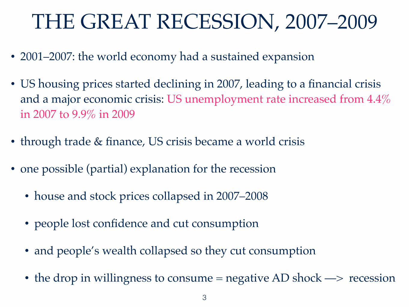
THE GREAT RECESSION, 2007–2009• 2001–2007: the world economy had a sustained expansion

• US housing prices started declining in 2007, leading to a financial crisis and a major economic crisis: US unemployment rate increased from 4.4% in 2007 to 9.9% in 2009

• through trade & finance, US crisis became a world crisis

• one possible (partial) explanation for the recession

• house and stock prices collapsed in 2007–2008

• people lost confidence and cut consumption

• and people’s wealth collapsed so they cut consumption

• the drop in willingness to consume = negative AD shock —> recession 3

Bubbles in housing prices?

1950 1960 1970 1980 1990 2000 2010

100

120

140

160

180

200

Year

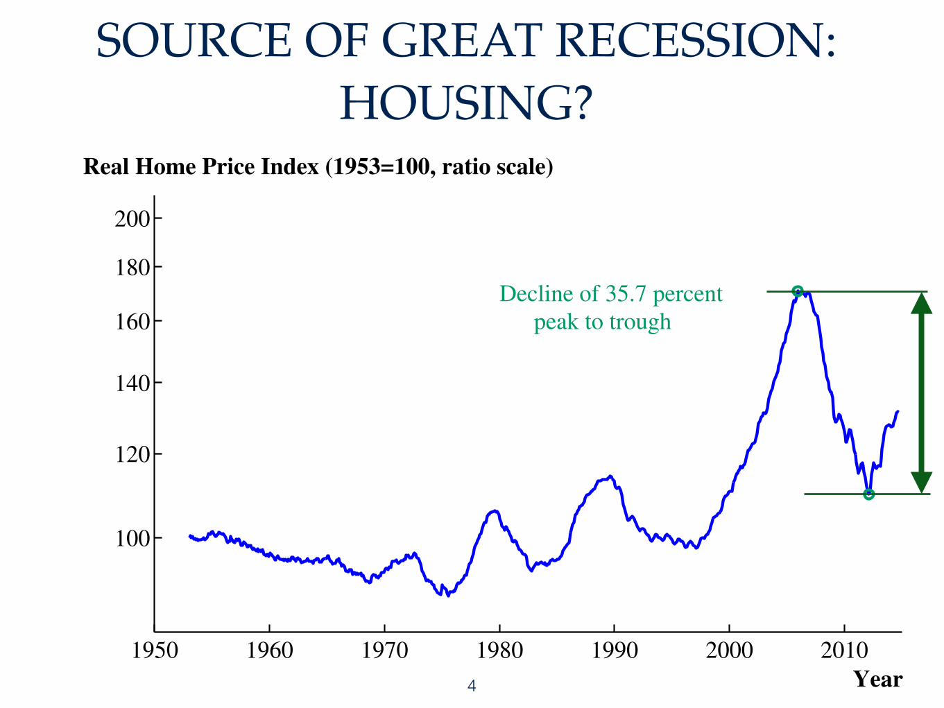
Real Home Price Index (1953=100, ratio scale)

Decline of 35.7 percentpeak to trough

Source: Robert Shiller, http://www.econ.yale.edu/~shiller/data.htm

Chad Jones, Updated Graphs – January 12, 2015 – p. 27

SOURCE OF GREAT RECESSION: HOUSING?

4

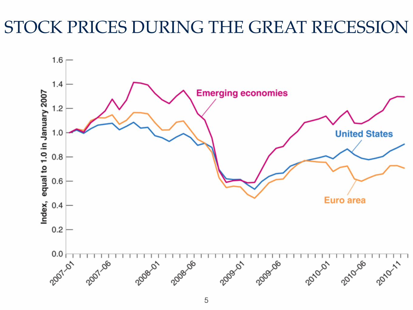
STOCK PRICES DURING THE GREAT RECESSION

5

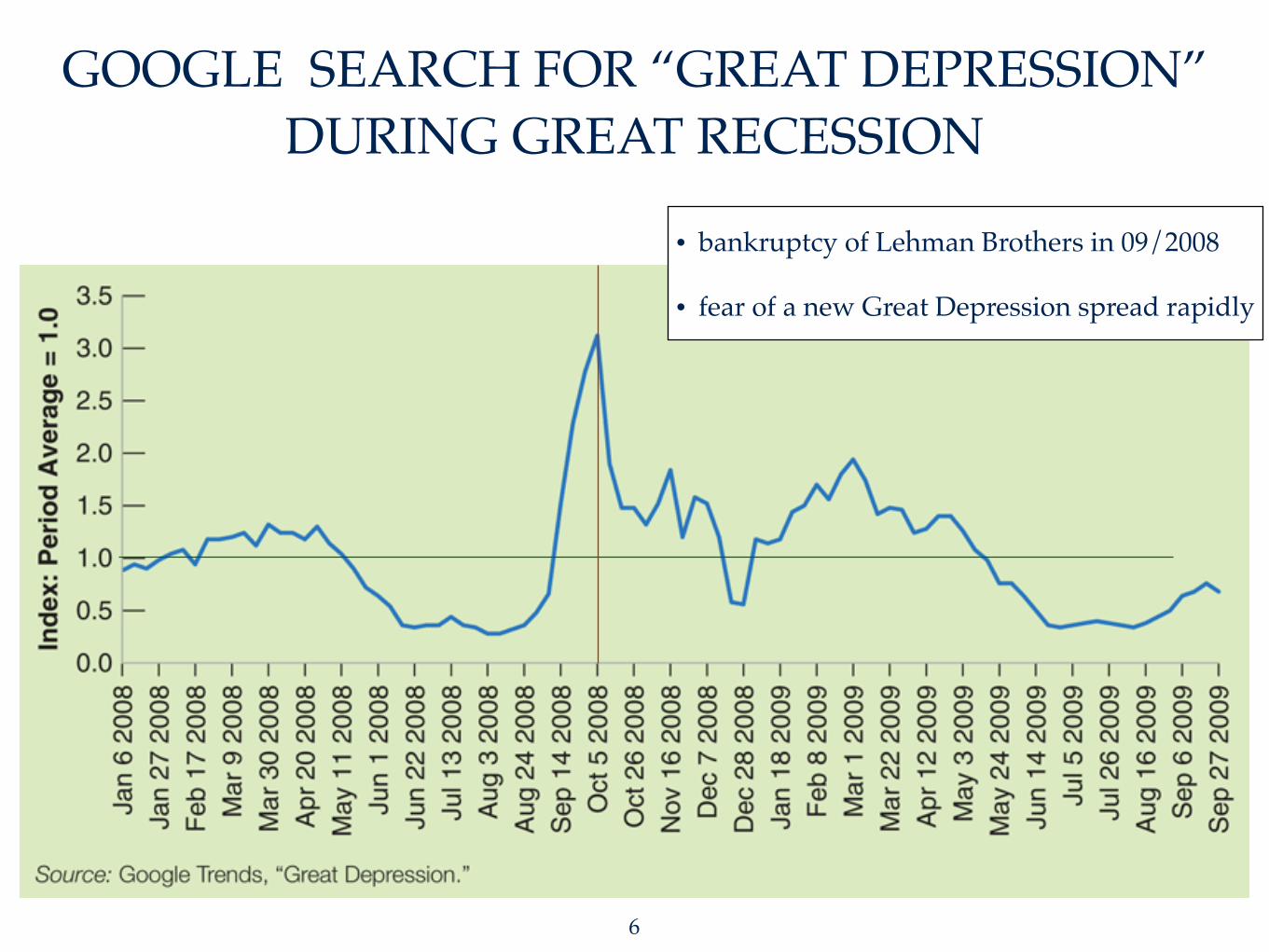
GOOGLE SEARCH FOR “GREAT DEPRESSION” DURING GREAT RECESSION

6

• bankruptcy of Lehman Brothers in 09/2008

• fear of a new Great Depression spread rapidly

DECLINE IN WILLINGNESS TO CONSUME

7

lower consumption but same disposable income indicates lower willingness to consume: lower c0 in consumption function

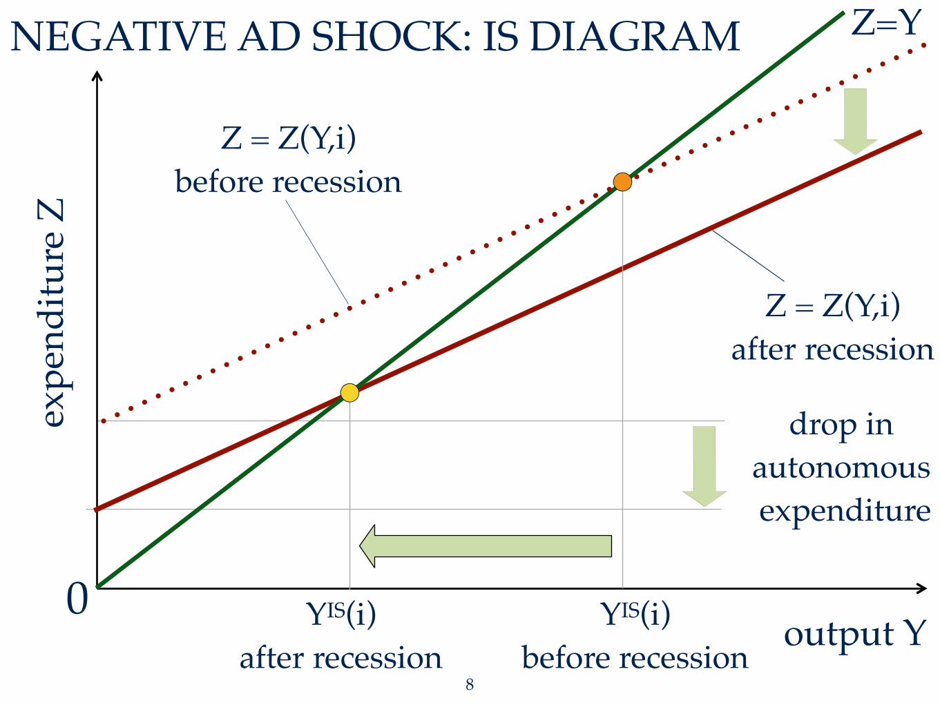
NEGATIVE AD SHOCK: IS DIAGRAM

8

expe

nditu

re Z

output Y0

Z = Z(Y,i)after recession

Z=Y

Z = Z(Y,i)before recession

drop in autonomous expenditure

YIS(i)after recession

YIS(i)before recession

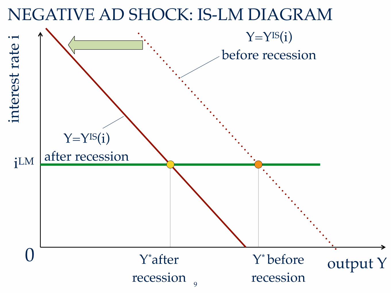
NEGATIVE AD SHOCK: IS-LM DIAGRAM

9

inte

rest

rate

i

output Y0

iLM

Y=YIS(i)after recession

Y=YIS(i)before recession

Y*afterrecession

Y* beforerecession

MANIFESTATION OF THE PARADOX OF THRIFT

• at the onset of Great Recession, consumers decided to save more, so c0 decreased

• private saving is S = – c0 + (1 – c1) x D

• autonomous expenditure decreased

• so equilibrium income in IS submodel decreased

• equilibrium income = autonomous expenditure × spending multiplier

• hence, at the onset of Great Recession, the IS curve shifted inward, while the LM curve stayed the same

10

MANIFESTATION OF THE PARADOX OF THRIFT

• IS-LM equilibrium: same interest rate i*, but lower GDP Y*

• hence investment I* = I(Y*,i*) fell

• the investment function I(Y,i) is increasing in Y but decreasing in i

• in equilibrium: private saving = investment – public saving

• public saving = T – G remained the same

• so paradoxically, since investment fell, private saving fell! 11

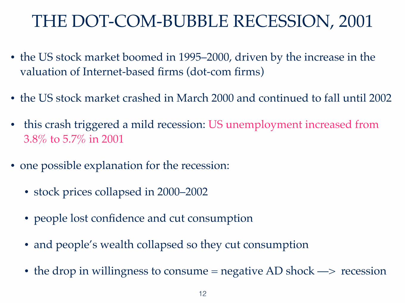
THE DOT-COM-BUBBLE RECESSION, 2001

• the US stock market boomed in 1995–2000, driven by the increase in the valuation of Internet-based firms (dot-com firms)

• the US stock market crashed in March 2000 and continued to fall until 2002

• this crash triggered a mild recession: US unemployment increased from 3.8% to 5.7% in 2001

• one possible explanation for the recession:

• stock prices collapsed in 2000–2002

• people lost confidence and cut consumption

• and people’s wealth collapsed so they cut consumption

• the drop in willingness to consume = negative AD shock —> recession

12

DOT-COM BUBBLE: NASDAQ

13