lecture 14 - aggregate demand ii. applying the is-lm model

8/12/2019 Lecture 14 - Aggregate Demand II. Applying the is-LM Model

http://slidepdf.com/reader/full/lecture-14-aggregate-demand-ii-applying-the-is-lm-model 1/25

Macroeconomics

Chapter 11 - Aggregate Demand II: Applyingthe IS-LM Model



In this chapter, you will learn

• How to use the IS-LM model to analyze theeffects of shocks, fiscal policy, and monetarypolicy

• How to derive the aggregate demand curvefrom the IS-LM model

• Several theories about what caused the GreatDepression



The intersection determinesthe unique combination of Y and r that satisfies equilibrium in both markets.

The LM curve representsmoney market equilibrium.

Equilibrium in the IS-LM ModelThe IS curve representsequilibrium in the goodsmarket.

( ) ( )Y C Y T I r G

( , )M P L r Y IS

Y

r LM

r 1

Y 1



Policy Analysis with the IS-LM Model

We can use the IS-LM modelto analyze the effects of

• Fiscal policy: G and/or T

• Monetary policy: M

( ) ( )Y C Y T I r G

( , )M P L r Y

IS

Y

r LM

r 1

Y 1



(lump-sum taxation)

causing output andincome to rise

IS 1

Increase in Government Purchases

1. IS curve shifts right

Y

r LM

r 1

Y 1

1by

1 MPCG

IS 2

Y 2

r 2

1.2. This raises moneydemand, causing the

interest rate to rise…

2.

3. …which reduces investment,so the final increase in Y

1is smaller than

1 MPC

G

3.



IS 1

1.

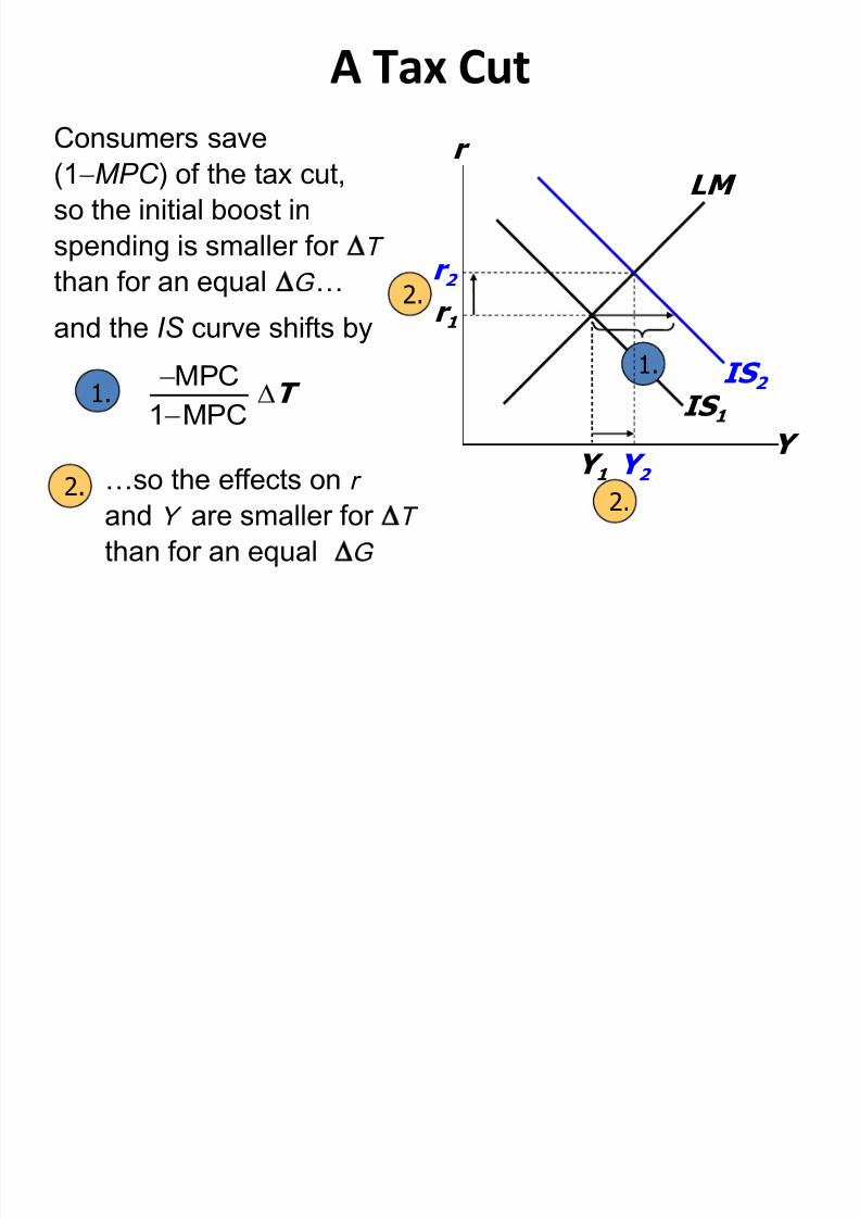
A Tax Cut

Y

r LM

r 1

Y 1

IS 2

Y 2

r 2

Consumers save(1 MPC ) of the tax cut,so the initial boost inspending is smaller for T than for an equal G …

and the IS curve shifts byMPC

1 MPCT 1.

2.

2.…so the effects on r and Y are smaller for T than for an equal G

2.



2. …causing theinterest rate to fall

IS

Monetary Policy: An Increase in M

1. M > 0 shiftsthe LM curve down(or to the right)

Y

r LM 1

r 1

Y 1 Y 2

r 2

LM 2

3. …which increases

investment, causingoutput and incometo rise



Practice: IS-LM

C(Y-T) = 200 + .75(Y-T)MPC = .75

t = 1/3I(r) = 2000 – 50r

G = 1300L(Y,r) = Y – 25r

M = 1000P = 1

Determine the IS and LM curves and then calculate theinterest rate (r) and income (Y) in equilibrium.



Interaction Between Monetary andFiscal Policy

• Model: Monetary and fiscal policy variables(M , G, and T ) are exogenous

• Real world: Monetary policymakers mayadjust M in response to changes in fiscalpolicy, or vice versa

• Such interaction may alter the impact of theoriginal policy change



The Fed’s Response to G > 0

• Suppose Congress increases G

• Possible Fed responses:1. hold M constant2. hold r constant

3. hold Y constant

• In each case, the effects of the G aredifferent…



If Congress raises G ,the IS curve shifts right.

IS 1

Response 1: Hold M Constant

Y

r LM 1

r 1

Y 1

IS 2

Y 2

r 2

If Fed holds M constant,

then LM curve doesn’tshift.

Results:

2 1Y Y Y

2 1r r r




IS 1

Response 2: Hold r Constant

Y

r LM 1

r 1

Y 1

IS 2

Y 2

r 2 To keep r constant,

Fed increases M to shift LM curve right.

3 1Y Y Y

0r

LM 2

Y 3

Results:



IS 1

Response 3: Hold Y Constant

Y

r LM 1

r 1

IS 2

Y 2

r 2 To keep Y constant,

Fed reduces M to shift LM curve left.

0Y

3 1r r r

LM 2

Results:

Y 1

r 3




Estimates of Fiscal Policy Multipliers

From the DRI macroeconometric model

Assumption aboutmonetary policy

Estimatedvalue of

Y / G

Fed holds nominalinterest rate constant

Fed holds moneysupply constant

1.93

0.60

Estimatedvalue of

Y / T

1.19

0.26



Shocks in the IS -LM model

LM shocks : exogenous changes in the demandfor money.

Examples:

– Wave of credit card fraud increases demand formoney

–More ATMs or the Internet reduce moneydemand



Practice: Analyzing Shocks

Use the IS-LM model to analyze the effects of:1. a boom in the stock market that makes consumers

wealthier.

2. after a wave of credit card fraud, consumers usingcash more frequently in transactions.

For each shock:a. use the IS-LM diagram to show the effects of the shock

on Y and r . b. determine what happens to C , I , and the

unemployment rate.



CASE STUDY:

The U.S. recession of 2001

• During 2001:

– 2.1 million jobs lost, unemployment rose from3.9% to 5.8%

– GDP growth slowed to 0.8% (compared to 3.9%

average annual growth during 1994-2000)



CASE STUDY:

The U.S. recession of 2001Causes: 1) Stock market decline C

300

600

900

1200

1500

1995 1996 1997 1998 1999 2000 2001 2002 2003

I n d e

x ( 1 9 4 2

= 1 0

0 ) Standard & Poor’s

500



CASE STUDY:


Causes: 2) 9/11 – Increased uncertainty

–Fall in consumer and business confidence

– Result: lower spending, IS curve shifted left

Causes: 3) Corporate accounting scandals – Enron, WorldCom, etc . – Reduced stock prices, discouraged investment



CASE STUDY:


• Fiscal policy response: shifted IS curve right

– Tax cuts in 2001 and 2003

– Spending increases

• Airline industry bailout

• NYC reconstruction• Afghanistan war



CASE STUDY:

The U.S. recession of 2001Monetary policy response: shifted LM curve right

Three-monthT-Bill Rate

0

1

2

34

5

6

7



Fed’s Policy Instrument

• The news media commonly report the Fed’s policychanges as interest rate changes, as if the Fed hasdirect control over market interest rates

• In fact, the Fed targets the federal funds rate – theinterest rate banks charge one another on overnightloans

• The Fed changes the money supply and shifts the LM

curve to achieve its target• Other short-term rates typically move with the federal

funds rate



Fed’s Policy Instrument

Why does the Fed target interest rates instead of themoney supply?

1) They are easier to measure than the moneysupply

2) The Fed might believe that LM shocks are moreprevalent than IS shocks. If so, then targeting the

interest rate stabilizes income better thantargeting the money supply



IS-LM and Aggregate Demand

• So far, we’ve been using the IS-LM model toanalyze the short run, when the price level isassumed fixed

• However, a change in P would shift LM andtherefore affect Y

• The aggregate demand curve captures thisrelationship between P and Y

lecture 14 - aggregate demand ii. applying the is-lm model

Documents