dmtm 2015 - 11 decision trees

Prof. Pier Luca Lanzi

Classification: Decision Trees !Data Mining and Text Mining (UIC 583 @ Politecnico di Milano)


The Weather Dataset

Outlook' Temp' Humidity' Windy' Play'

Sunny' Hot' High' False' No'

Sunny' Hot'' High'' True' No'

Overcast'' Hot''' High' False' Yes'

Rainy' Mild' High' False' Yes'

Rainy' Cool' Normal' False' Yes'

Rainy' Cool' Normal' True' No'

Overcast' Cool' Normal' True' Yes'

Sunny' Mild' High' False' No'

Sunny' Cool' Normal' False' Yes'

Rainy' Mild' Normal' False' Yes'

Sunny' Mild' Normal' True' Yes'

Overcast' Mild' High' True' Yes'

Overcast' Hot' Normal' False' Yes'

Rainy' Mild' High' True' No'

2


The Decision Tree for the !Weather Dataset

3

humidity

overcast

No NoYes Yes

Yes

outlook

windy

sunny rain

falsetruenormalhigh


What is a Decision Tree?

•  An internal node is a test on an attribute

•  A branch represents an outcome of the test, e.g., outlook=windy

•  A leaf node represents a class label or class label distribution

•  At each node, one attribute is chosen to split training examples into distinct classes as much as possible

•  A new case is classified by following a matching path to a leaf node

4


Building a Decision Tree with KNIME


Decision Tree Representations (Graphical) 8


Decision Tree Representations (Text)

outlook = overcast: yes {no=0, yes=4} outlook = rainy | windy = FALSE: yes {no=0, yes=3}| windy = TRUE: no {no=2, yes=0} outlook = sunny | humidity = high: no {no=3, yes=0} | humidity = normal: yes {no=0, yes=2}

9


Computing Decision Trees


Computing Decision Trees

•  Top-down Tree Construction! Initially, all the training examples are at the root! Then, the examples are recursively partitioned, !

by choosing one attribute at a time

•  Bottom-up Tree Pruning! Remove subtrees or branches, in a bottom-up manner, to

improve the estimated accuracy on new cases.

11


Top Down Induction of Decision Trees

function TDIDT(S) // S, a set of labeled examples

Tree = new empty node

if (all examples have the same class c

or no further splitting is possible)

then // new leaf labeled with the majority class c

Label(Tree) = c

else // new decision node

(A,T) = FindBestSplit(S)

foreach test t in T do

St = all examples that satisfy t

Nodet = TDIDT(St)

AddEdge(Tree -> Nodet)

endfor

endif

return Tree

12


When Should Building Stop?

•  There are several possible stopping criteria

•  All samples for a given node belong to the same class

•  If there are no remaining attributes for further partitioning, majority voting is employed

•  There are no samples left

•  Or there is nothing to gain in splitting

13


How is the Splitting Attribute Determined?


What Do We Need? 15

k

IF salary<k THEN not repaid


Which Attribute for Splitting?

•  At each node, available attributes are evaluated on the basis of separating the classes of the training examples

•  A purity or impurity measure is used for this purpose

•  Information Gain: increases with the average purity of the subsets that an attribute produces

•  Splitting Strategy: choose the attribute that results in greatest information gain

•  Typical goodness functions: information gain (ID3), information gain ratio (C4.5), gini index (CART)

16


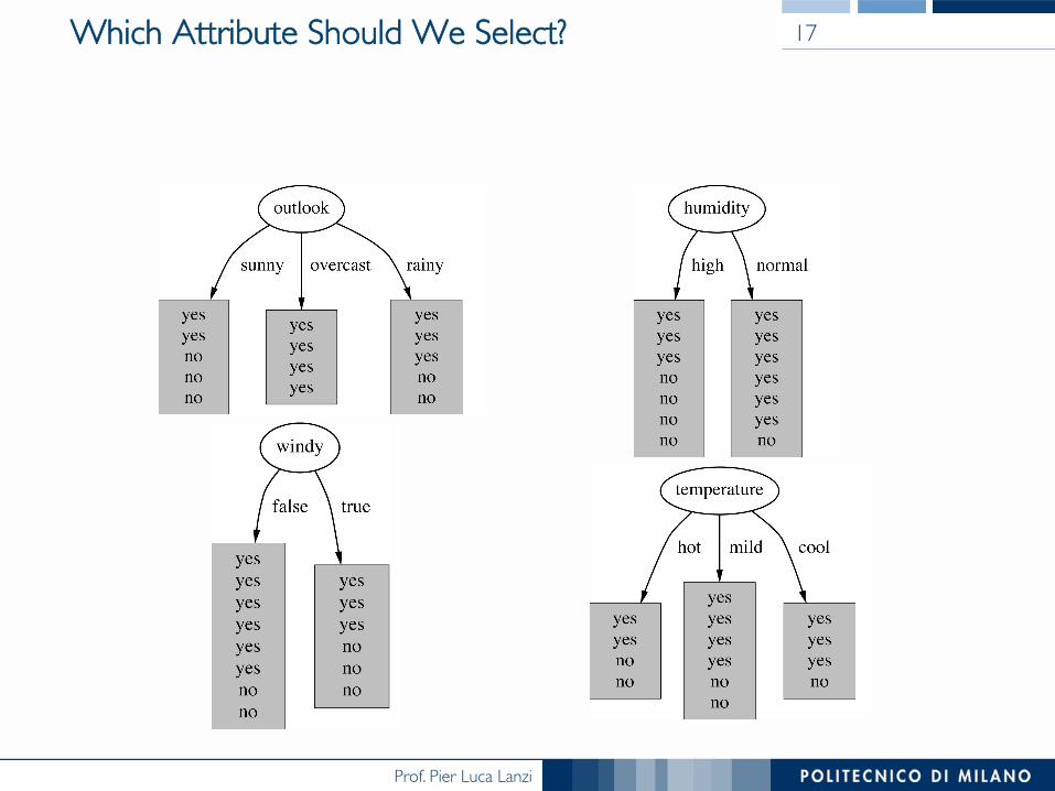
Which Attribute Should We Select? 17


Computing Information

•  Information is measured in bits! Given a probability distribution, the info required to predict an

event is the distribution’s entropy! Entropy gives the information required in bits (this can involve

fractions of bits!)

•  Formula for computing the entropy

18


Entropy 19

two classes 0/1

% of elements of class 0

entr

opy


Which Attribute Should We Select? 20


The Attribute “outlook”

•  outlook” = “sunny”

•  “outlook” = “overcast”

•  “outlook” = “rainy”

•  Expected information for attribute

21


Information Gain

•  Difference between the information before split and the information after split

•  The information before the split, info(D), is the entropy,

•  The information after the split using attribute A is computed as the weighted sum of the entropies on each split, given n splits,

22


Information Gain

•  Difference between the information before split and the information after split

•  Information gain for the attributes from the weather data:! gain(“outlook”)=0.247 bits! gain(“temperature”)=0.029 bits! gain(“humidity”)=0.152 bits! gain(“windy”)=0.048 bits

23


You can check the math using KNIME


Going Further 26


The Final Decision Tree

•  Not all the leaves need to be pure•  Splitting stops when data can not be split any further

27


We Can Always Build a 100% Accurate Tree…


Another Version of the Weather Dataset

ID Code Outlook Temp Humidity Windy Play

A Sunny Hot High False NoB Sunny Hot High True NoC Overcast Hot High False YesD Rainy Mild High False YesE Rainy Cool Normal False YesF Rainy Cool Normal True NoG Overcast Cool Normal True YesH Sunny Mild High False NoI Sunny Cool Normal False YesJ Rainy Mild Normal False YesK Sunny Mild Normal True YesL Overcast Mild High True YesM Overcast Hot Normal False YesN Rainy Mild High True No

31


Decision Tree for the New Dataset

•  Entropy for splitting using “ID Code” is zero, since each leaf node is “pure”•  Information Gain is thus maximal for ID code

32


Highly-Branching Attributes

•  Attributes with a large number of values are usually problematic

•  Examples: id, primary keys, or almost primary key attributes

•  Subsets are likely to be pure if there is a large number of values

•  Information Gain is biased towards choosing attributes with a large number of values

•  This may result in overfitting (selection of an attribute that is non-optimal for prediction)

33


Information Gain Ratio


Information Gain Ratio

•  Modification of the Information Gain that reduces the bias toward highly-branching attributes

•  Information Gain Ratio should be ! Large when data is evenly spread! Small when all data belong to one branch

•  Information Gain Ratio takes number and size of branches into account when choosing an attribute

•  It corrects the information gain by taking the intrinsic information of a split into account

35


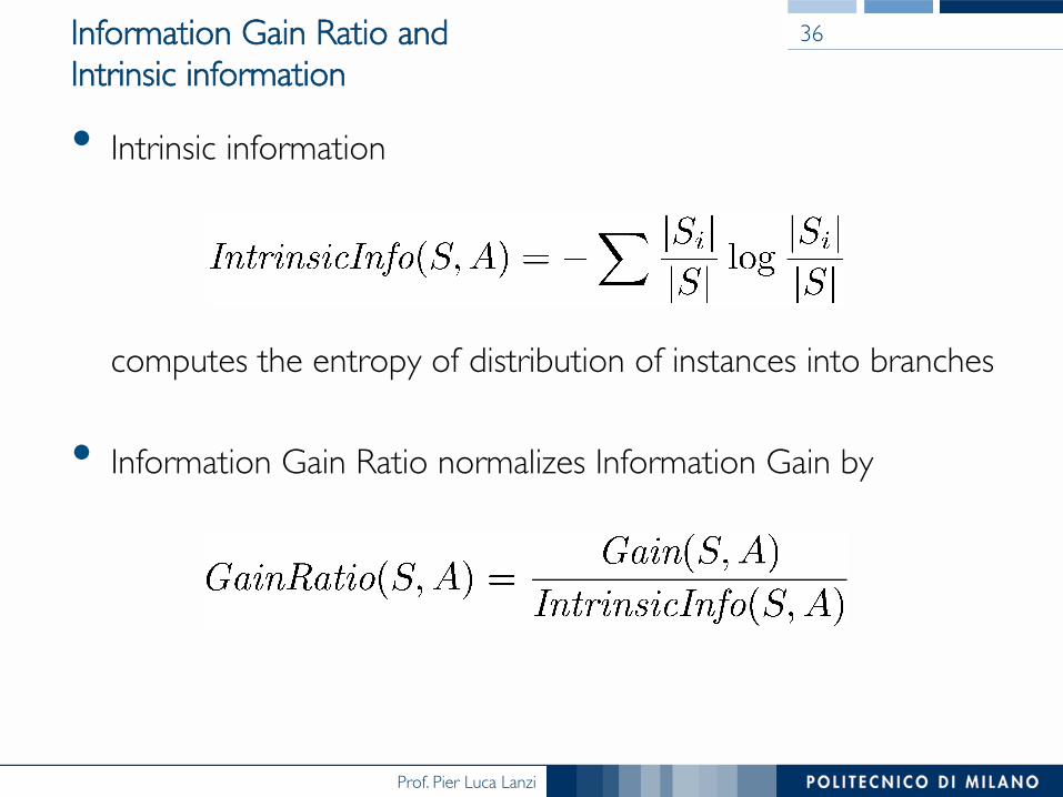
Information Gain Ratio and !Intrinsic information

•  Intrinsic information !!!!!computes the entropy of distribution of instances into branches

•  Information Gain Ratio normalizes Information Gain by

36


Computing the Information Gain Ratio

•  The intrinsic information for ID code is

•  Importance of attribute decreases as intrinsic information gets larger

•  The Information gain ratio of “ID code”,

37


Information Gain Ratio for Weather Data 38

Outlook TemperatureInfo: 0.693 Info: 0.911Gain: 0.940-0.693 0.247 Gain: 0.940-0.911 0.029Split info: info([5,4,5]) 1.577 Split info: info([4,6,4]) 1.362Gain ratio: 0.247/1.577 0.156 Gain ratio: 0.029/1.362 0.021

Humidity WindyInfo: 0.788 Info: 0.892Gain: 0.940-0.788 0.152 Gain: 0.940-0.892 0.048Split info: info([7,7]) 1.000 Split info: info([8,6]) 0.985Gain ratio: 0.152/1 0.152 Gain ratio: 0.048/0.985 0.049


More on Information Gain Ratio

•  “outlook” still comes out top, however “ID code” has greater Information Gain Ratio

•  The standard fix is an ad-hoc test to prevent splitting on that type of attribute

•  First, only consider attributes with greater than average Information Gain; Then, compare them using the Information Gain Ratio

•  Information Gain Ratio may overcompensate and choose an attribute just because its intrinsic information is very low

39


What if Attributes are Numerical?


The Weather Dataset (Numerical)

Outlook Temp Humidity Windy PlaySunny 85 85 False NoSunny 80 90 True No

Overcast 83 78 False YesRainy 70 96 False YesRainy 68 80 False YesRainy 65 70 True No

Overcast 64 65 True YesSunny 72 95 False NoSunny 69 70 False YesRainy 75 80 False YesSunny 75 70 True Yes

Overcast 72 90 True YesOvercast 81 75 False Yes

Rainy 71 80 True No

41


The Temperature Attribute

•  First, sort the temperature values, including the class labels•  Then, check all the cut points and choose the one with the best

information gain

•  E.g. temperature < 71.5: yes/4, no/2 !temperature ≥ 71.5: yes/5, no/3

•  Info([4,2],[5,3]) = 6/14 info([4,2]) + 8/14 info([5,3]) = 0.939•  Place split points halfway between values•  Can evaluate all split points in one pass!

64 65 68 69 70 71 72 72 75 75 80 81 83 85 Yes No Yes Yes Yes No No Yes Yes Yes No Yes Yes No


The Information Gain for Humidity

Humidity' Play'

65 Yes'70 No'70 Yes'70 Yes'75 Yes'78 Yes'80 Yes'80 Yes'80 No'85 No'90 No'90 Yes'95 No'96 Yes'

43

Humidity' Play'

65 Yes'70 No'70 Yes'70 Yes'75 Yes'78 Yes'80 Yes'80 Yes'80 No'85 No'90 No'90 Yes'95 No'96 Yes'

sort the attribute

values

compute the gain for every possible split

what is the information gain if we split here?


Information Gain for Humidity

Humidity Play # of Yes % of Yes # of No % of No Weight Entropy

Left# of Yes % of Yes # of

No% of No Weight Entropy

RightInformation

Gain65 Yes 1 100.00% 0 0.00% 7.14% 0.00 8.00 0.62 5.00 0.38 92.86% 0.96 0.047770 No 1 50.00% 1 50.00% 14.29% 1.00 8.00 0.67 4.00 0.33 85.71% 0.92 0.010370 Yes 2 66.67% 1 33.33% 21.43% 0.92 7.00 0.64 4.00 0.36 78.57% 0.95 0.000570 Yes 3 75.00% 1 25.00% 28.57% 0.81 6.00 0.60 4.00 0.40 71.43% 0.97 0.015075 Yes 4 80.00% 1 20.00% 35.71% 0.72 5.00 0.56 4.00 0.44 64.29% 0.99 0.045378 Yes 5 83.33% 1 16.67% 42.86% 0.65 4.00 0.50 4.00 0.50 57.14% 1.00 0.090380 Yes 6 85.71% 1 14.29% 50.00% 0.59 3.00 0.43 4.00 0.57 50.00% 0.99 0.151880 Yes 7 87.50% 1 12.50% 57.14% 0.54 2.00 0.33 4.00 0.67 42.86% 0.92 0.236180 No 7 77.78% 2 22.22% 64.29% 0.76 2.00 0.40 3.00 0.60 35.71% 0.97 0.102285 No 7 70.00% 3 30.00% 71.43% 0.88 2.00 0.50 2.00 0.50 28.57% 1.00 0.025190 No 7 63.64% 4 36.36% 78.57% 0.95 2.00 0.67 1.00 0.33 21.43% 0.92 0.000590 Yes 8 66.67% 4 33.33% 85.71% 0.92 1.00 0.50 1.00 0.50 14.29% 1.00 0.010395 No 8 61.54% 5 38.46% 92.86% 0.96 1.00 1.00 0.00 0.00 7.14% 0.00 0.047796 Yes 9 64.29% 5 35.71% 100.00% 0.94 0.00 0.00 0.00 0.00 0.00% 0.00 0.0000

44


Otherwise, we can discretize…


Discretization

•  Processing for converting an interval/numerical variable into a a finite (discrete) set of elements (labels)

•  A discretization algorithm computes a series of cut-points which defines a set of intervals that are mapped into labels

•  Motivations: many methods (also in mathematics and computer science) cannot deal with numerical variables. In these cases, discretization is required to be able to use them, despite the loss of information

•  Several approaches! Supervised vs unsupervised! Static vs dynamic

46


Unsupervised vs Supervised Discretization

•  Unsupervised discretization just uses the attribute values, for instance, discretize humidity as <70, 70-79, >=80)

•  Supervised discretization also uses the class attribute to generate interval with lower entropy

•  Example using humidity! Values alone may suggest <60, 60-70

! Considering the class value might suggest different intervals!!!!by grouping values to maintain information about the class attribute

47

64 65 68 69 70 71 72 72 75 75 80 81 83 85

64 65 68 69 70 71 72 72 75 75 80 81 83 85 Yes | No | Yes Yes Yes | No No | Yes | Yes Yes | No | Yes Yes | No


Example of Unsupervised and Supervised Discretization for Humidity

48

Unsupervised Discretization Supervised Discretization


The Gini Index


Another Splitting Criteria: !The Gini Index

•  The gini index, for a data set T contains examples from n classes, is defined as!!!!!where pj is the relative frequency of class j in T

•  gini(T) is minimized if the classes in T are skewed.

50


The Gini Index vs Entropy 51


The Gini Index

•  If a data set D is split on A into two subsets D1 and D2, then,

•  The reduction of impurity is defined as,

•  The attribute provides the smallest gini splitting D over A (or the largest reduction in impurity) is chosen to split the node (need to enumerate all the possible splitting points for each attribute)

52


The Gini Index: Example

•  D has 9 tuples labeled “yes” and 5 labeled “no”

•  Suppose the attribute income partitions D into 10 in D1 branching on low and medium and 4 in D2

•  but gini{medium,high} is 0.30 and thus the best since it is the lowest

53


Generalization and Overfitting in Decision Trees


Avoiding Overfitting in Decision Trees

•  The generated tree may overfit the training data

•  Too many branches, some may reflect anomalies !due to noise or outliers

•  Result is in poor accuracy for unseen samples

•  Two approaches to avoid overfitting! Prepruning! Postpruning

57


Pre-pruning vs Post-pruning

•  Prepruning! Halt tree construction early! Do not split a node if this would result in the goodness

measure falling below a threshold! Difficult to choose an appropriate threshold

•  Postpruning! Remove branches from a “fully grown” tree! Get a sequence of progressively pruned trees! Use a set of data different from the training data to decide

which is the “best pruned tree”

58


Pre-Pruning

•  Based on statistical significance test

•  Stop growing the tree when there is no statistically significant association between any attribute and the class at a particular node

•  Early stopping and halting! No individual attribute exhibits any interesting information

about the class! The structure is only visible in fully expanded tree! Pre-pruning won’t expand the root node

59


Post-Pruning

•  First, build full tree, then prune it•  Fully-grown tree shows all attribute interactions •  Problem: some subtrees might be due to chance effects

•  Two pruning operations! Subtree raising ! Subtree replacement

•  Possible strategies! Error estimation! Significance testing! MDL principle

60


Subtree Raising

•  Delete node•  Redistribute instances•  Slower than subtree replacement

61

X


Subtree Replacement

• Works bottom-up•  Consider replacing a tree !

only after considering !all its subtrees

62


Estimating Error Rates

•  Prune only if it reduces the estimated error

•  Error on the training data is NOT a useful estimator !(Why it would result in very little pruning?)

•  A hold-out set might be kept for pruning!(“reduced-error pruning”)

•  Example (C4.5’s method)! Derive confidence interval from training data! Use a heuristic limit, derived from this, for pruning! Standard Bernoulli-process-based method! Shaky statistical assumptions (based on training data)

63


Mean and Variance

•  Mean and variance for a Bernoulli trial: p, p (1–p)

•  Expected error rate f=S/N has mean p and variance p(1–p)/N

•  For large enough N, f follows a Normal distribution

•  c% confidence interval [–z ≤ X ≤ z] for random variable with 0 mean is given by:

• With a symmetric distribution,

64


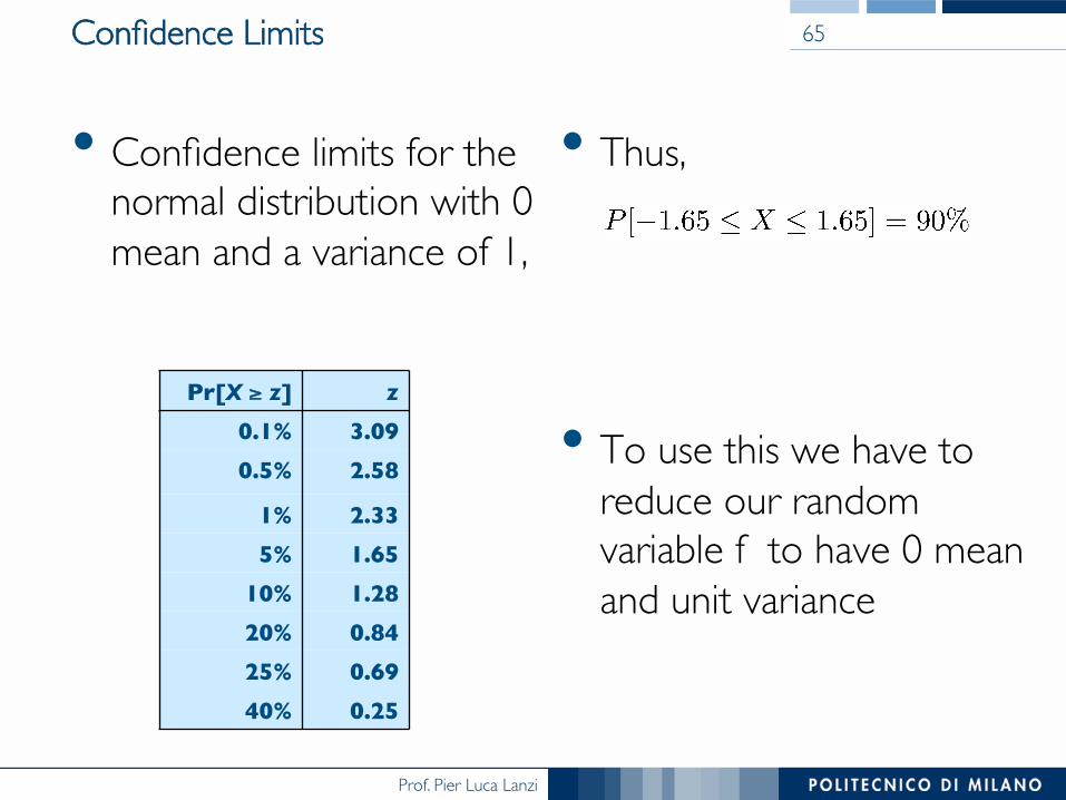
Confidence Limits

• Confidence limits for the normal distribution with 0 mean and a variance of 1,

• Thus,

• To use this we have to reduce our random variable f to have 0 mean and unit variance

65

Pr[X ≥ z] z

0.1% 3.09

0.5% 2.58

1% 2.33

5% 1.65

10% 1.28

20% 0.84

25% 0.69

40% 0.25


C4.5’s Pruning Method

•  Given the error f on the training data, the upper bound for the error estimate for a node is computed as

•  If c = 25% then z = 0.69 (from normal distribution)! f is the error on the training data! N is the number of instances covered by the leaf

66

!"

#$%

&+!

!"

#$$%

&+−++=

Nz

Nz

Nf

Nf

zNz

fe2

2

222

142


f=0.33 e=0.47

f=0.5 e=0.72

f=0.33 e=0.47

f = 5/14 e = 0.46 e < 0.51 so prune!

Combined using ratios 6:2:6 gives 0.51


Examples Using KNIME


pruned tree (Gain ratio)


pruned tree (Gini index)


Regression Trees


Regression Trees for Prediction

•  Decision trees can also be used to predict the value of a numerical target variable•  Regression trees work similarly to decision trees, by analyzing

several splits attempted, choosing the one that minimizes impurity•  Differences from Decision Trees! Prediction is computed as the average of numerical target

variable in the subspace (instead of the majority vote)! Impurity is measured by sum of squared deviations from leaf

mean (instead of information-based measures)! Find split that produces greatest separation in [y – E(y)]2 ! Find nodes with minimal within variance and therefore! Performance is measured by RMSE (root mean squared error)

72


00

32128

CHMAX

00

816

CHMIN

Channels PerformanceCache (Kb)

Main memory (Kb)

Cycle time (ns)

4504000100048020967328000512480208

…2693232000800029219825660002561251PRPCACHMMAXMMINMYCT

PRP = -55.9 + 0.0489 MYCT + 0.0153 MMIN + 0.0056 MMAX + 0.6410 CACH - 0.2700 CHMIN + 1.480 CHMAX


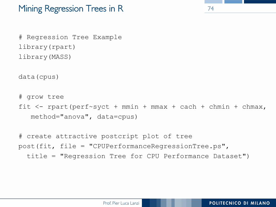
Mining Regression Trees in R

# Regression Tree Example library(rpart) library(MASS) data(cpus) # grow tree fit <- rpart(perf~syct + mmin + mmax + cach + chmin + chmax, method="anova", data=cpus) # create attractive postcript plot of tree post(fit, file = "CPUPerformanceRegressionTree.ps", title = "Regression Tree for CPU Performance Dataset")

74


|

mmax< 2.8e+04

cach< 27

cach< 96.5

cach< 80

mmax>=2.8e+04

cach>=27

cach>=96.5

cach>=80

105.62n=209

60.72n=182

39.638n=141

133.22n=41

114.44n=34

224.43n=7

408.26n=27

299.21n=19

667.25n=8

Regression Tree for CPU Performance Dataset


Summary


Summary

•  Decision tree construction is a recursive procedure involving! The selection of the best splitting attribute! (and thus) a selection of an adequate purity measure

(Information Gain, Information Gain Ratio, Gini Index)! Pruning to avoid overfitting

•  Information Gain is biased toward highly splitting attributes•  Information Gain Ratio takes the number of splits that an

attribute induces into the picture but might not be enough

77


Suggested Homework

•  Try building the tree for the nominal version of the Weather dataset using the Gini Index

•  Compute the best upper bound you can for the computational complexity of the decision tree building

•  Check the problems given in the previous year exams on the use of Information Gain, Gain Ratio and Gini index, solve them and check the results using Weka.

78

dmtm 2015 - 11 decision trees

Education