dl poly/field/meso tutorial - prace training … · dl_poly/field/meso tutorial software solutions...
TRANSCRIPT

Autumn School, Sofia
Bulgaria 2012
DL_POLY/FIELD/MESO TUTORIAL
Software Solutions in Atomistic Modelling
ILIAN TODOROV
CHIN YONG, MICHAEL SEATON
CSED, STFC DARESBURY LABORATORY, DARESBURY
WARRINGTON WA4 4AD, CHESHIRE, ENGLAND, UK

Autumn School, Sofia
Bulgaria 2012
Daresbury Laboratory
Alice’s Wonderland (1865)
Lewis Carroll (Charles Lutwidge Dodgson)

Autumn School, Sofia
Bulgaria 2012
Multiple Scales of Materials Modelling

Autumn School, Sofia
Bulgaria 2012
Part 1
DL_POLY Project Background

Autumn School, Sofia
Bulgaria 2012
DL_POLY Trivia
• General purpose parallel (classical) MD simulation software
• It was conceived to meet needs of CCP5 - The Computer
Simulation of Condensed Phases (academic collaboration
community)
• Written in modularised Fortran90 (NagWare & FORCHECK
compliant) with MPI2 (MPI1+MPI-I/O) & fully self-contained
• 1994 – 2012: DL_POLY_2 (RD) by W. Smith & T.R. Forester
(funded for 6 years by EPSRC at DL). Now moved to a BSD
open source licence as DL_POLY_Classic.
• 2003 – 2012: DL_POLY_3 (DD) by I.T. Todorov & W. Smith
(funded for 4 years by NERC at Cambridge). Up-licensed to
DL_POLY_4 in 2010 - free of charge to academic
researchers and at cost to industry (provided as source).
• ~ 14,000 licences taken out since 1994 (~1,600 annually)
• ~ 1,200 registered FORUM members since 2005

Autumn School, Sofia
Bulgaria 2012
Written in modularised free formatted F90 (+MPI) with rigorous
code syntax (FORCHECK and NAGWare verified) and no external
library dependencies
• DL_POLY_4 (version 3.2)
– Domain Decomposition parallelisation, based on domain
decomposition (no dynamic load balancing), limits: up to
≈2.1×10⁹ atoms with inherent parallelisation
– Parallel I/O (amber netCDF) and radiation damage features
– Free format (flexible) reading with some fail-safe features
and basic reporting (but not fully fool-proofed)
• DL_POLY Classic (version 1.9)
– Replicated Data parallelisation, limits up to ≈30,000 atoms
with good parallelisation up to 100 (system dependent)
processors (running on any processor count)
– Hyper-dynamics, Temperature Accelerated Dynamics,
Solvation Dynamics, Path Integral MD
– Free format reading (somewhat rigid)
Current Versions

Autumn School, Sofia
Bulgaria 2012
DL_POLY on the Web
WWW:
http://www.ccp5.ac.uk/DL_POLY/
FTP:
ftp://ftp.dl.ac.uk/ccp5/DL_POLY/
DEV:
http://ccpforge.cse.rl.ac.uk/gf/project/dl-poly/
http://ccpforge.cse.rl.ac.uk/gf/project/dl_poly_classic/
FORUM:
http://www.cse.stfc.ac.uk/disco/forums/ubbthreads.php/

Autumn School, Sofia
Bulgaria 2012
W. Smith and T.R. Forester,
J. Molec. Graphics (1996), 14, 136
W. Smith, C.W. Yong, P.M. Rodger,
Molecular Simulation (2002), 28, 385
I.T. Todorov, W. Smith, K. Trachenko, M.T. Dove,
J. Mater. Chem. (2006), 16, 1611-1618
W. Smith (Guest Editor),
Molecular Simulation (2006), 32, 933
I.J. Bush, I.T. Todorov and W. Smith,
Comp. Phys. Commun. (2006), 175, 323-329
Further Information

Autumn School, Sofia
Bulgaria 2012
DL_POLY_DD Development Statistics
0
20
40
60
80
100
120
140
2002 2004 2006 2008 2010 2012 2014
Pu
bli
sh
ed
lin
es o
f co
de [
x 1
,000]
Year

Autumn School, Sofia
Bulgaria 2012
DL_POLY Licence Statistics
0
400
800
1200
1600
1992 1996 2000 2004 2008 2012
Do
wn
load
s
Year
Licences

Autumn School, Sofia
Bulgaria 2012
DL_POLY Licence Statistics
Asia38%
EU-REST17%
North America22%
UK11%
Latin America4%
Europe-REST5%
Africa2%
Australia and New Zealand and Philipnes
1%
DL_POLY Licences2010 by Sub-Areas
Asia39%
EU-REST19%
North America15%
UK10%
Latin America8%
Europe-REST4%
Africa3%
Australia and New Zealand and Philipnes
2%
DL_POLY Licences2011 by Sub-Areas

Autumn School, Sofia
Bulgaria 2012
DL_POLY Licence Statistics
Bio-Chemsitry5%
Chemistry33%
Engineering13%
Mechanics10%
Other1%
Physics33%
Software5%
DL_POLY Licences2010 by Science Domain
Bio-Chemsitry4%
Chemistry38%
Engineering17%
Materials7%Mechanics
3%
Other3%
Physics28%
DL_POLY Licences2011 by Science Domain

Autumn School, Sofia
Bulgaria 2012
Part 2
The Molecular Dynamics Method

Autumn School, Sofia
Bulgaria 2012
Molecular Dynamics: Definitions
• Theoretical tool for modelling the detailed microscopic behaviour
of many different types of systems, including; gases, liquids, solids,
polymers, surfaces and clusters.
• In an MD simulation, the classical equations of motion governing
the microscopic time evolution of a many body system are solved
numerically, subject to the boundary conditions appropriate for the
geometry or symmetry of the system.
• Can be used to monitor the microscopic mechanisms of energy
and mass transfer in chemical processes, and dynamical properties
such as absorption spectra, rate constants and transport properties
can be calculated.
• Can be employed as a means of sampling from a statistical
mechanical ensemble and determining equilibrium properties.
These properties include average thermodynamic quantities
(pressure, volume, temperature, etc.), structure, and free energies
along reaction paths.

Autumn School, Sofia
Bulgaria 2012
MD simulations are used for:
• Microscopic insight: we can follow the
motion of a single molecule (glass of
water)
• Investigation of phase change (NaCl)
• Understanding of complex systems like
polymers (plastics – hydrophilic and
hydrophobic behaviour)
Molecular Dynamics for Beginners
Autumn School, Sofia
Bulgaria 2012
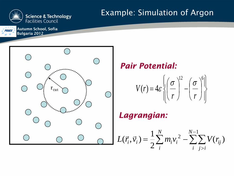
Example: Simulation of Argon
rcut
612
4)(rr
rV
Pair Potential:
Lagrangian:
L r v m v V ri i i ii
N
ijj ii
N
( , ) ( )
1
2
21

Autumn School, Sofia
Bulgaria 2012
Lennard -Jones Potential
612
4)(rr
rV
V(r)
r
rcut
Pair-wise radial distance

Autumn School, Sofia
Bulgaria 2012
Equations of Motion
d
dt
L
v
L
ri i
)( ijiij
N
ij
iji
iii
rVf
fF
Fam
Lagrange Equation –
time evolution
Force Evaluation –
particle interactions

Autumn School, Sofia
Bulgaria 2012
Boundary Conditions
• None – biopolymer
simulations
• Stochastic boundaries
– biopolymers
• Hard wall boundaries
– pores, capillaries
• Periodic boundaries –
most MD simulations
2D cubic periodic

Autumn School, Sofia
Bulgaria 2012
Periodic Boundary Conditions
Triclinic
Truncated octahedron
Hexagonal prism
Rhombic dodecahedron

Autumn School, Sofia
Bulgaria 2012
• Kinetic Energy:
• Temperature:
• Configuration Energy:
• Pressure:
• Specific heat:
K E m vi ii
N
. . 1
2
2
TNk
K EB
2
3. .
U V rc ijj i
N
i
( )
N
i
iiB frTNkPV
3
1
v
BB
NVEc
C
NkTNkU
2
31
2
3)( 222
System Properties: Static (1)

Autumn School, Sofia
Bulgaria 2012
Structural Properties
– Pair correlation (Radial Distribution Function):
– Structure factor:
– Note: S(k) available from x-ray diffraction
System Properties: Static (2)
g rn r
r r
V
Nr rij
j i
N
i
( )( )
( )
4 2 2
drrrgkr
krkS 2
01)(
)sin(41)(

Autumn School, Sofia
Bulgaria 2012
R
R
Radial Distribution Function (RDF)
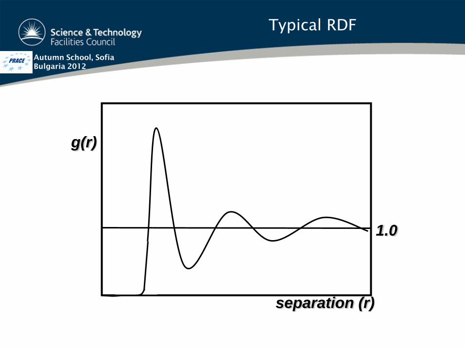
Autumn School, Sofia
Bulgaria 2012
g(r)
separation (r)
1.0
Typical RDF

Autumn School, Sofia
Bulgaria 2012
System Properties: Dynamic
Single Correlation Functions:
• Mean Square Displacement (Einstein
Relation)
• Velocity Autocorrelation (Green-Kubo
relation)

Autumn School, Sofia
Bulgaria 2012
System Properties: Collective
Collective Correlation Functions:
• van Hove correlation functions (general,
self, distinct)
• Particle density
• Intermediate scattering function
• Dynamic structure factor

Autumn School, Sofia
Bulgaria 2012
Correlation Function Uses
• Complete description of bulk dynamical
properties
• Space-time Fourier Transform of van Hove
function
• Elastic properties of materials
• Energy dissipation
• Sound propagation
Obtained directly from neutron scattering

Autumn School, Sofia
Bulgaria 2012
Part 2
DL_POLY Basics & Algorithms

Autumn School, Sofia
Bulgaria 2012
Point ions
and atoms
Polarisable
ions (core+
shell) Flexible
molecules Rigid
bonds
Rigid
molecules
Flexibly
linked rigid
molecules
Rigid bond
linked rigid
molecules
DL_POLY Supported Molecular Entities

Autumn School, Sofia
Bulgaria 2012
Force Field Definitions – I
• particle: rigid ion or atom (charged or not), a core or a shell of a
polarisable ion(with or without associated degrees of freedom), a
massless charged site. A particle is a countable object and has a
global ID index.
• site: a particle prototype that serves to defines the chemical &
physical nature (topology/connectivity/stoichiometry) of a particle
(mass, charge, frozen-ness). Sites are not atoms they are
prototypes!
• Intra-molecular interactions: chemical bonds, bond angles,
dihedral angles, improper dihedral angles, inversions. Usually, the
members in a unit do not interact via an inter-molecular term.
However, this can be overridden for some interactions. These are
defined by site.
• Inter-molecular interactions: van der Waals, metal (EAM, Gupta,
Finnis-Sinclair, Sutton-Chen), Tersoff, three-body, four-body.
Defined by species.

Autumn School, Sofia
Bulgaria 2012
Force Field Definitions – II
• Electrostatics: Standard Ewald*, Hautman-Klein (2D) Ewald*,
SPM Ewald (3D FFTs), Force-Shifted Coulomb, Reaction Field,
Fennell damped FSC+RF, Distance dependent dielectric constant,
Fuchs correction for non charge neutral MD cells.
• Ion polarisation via Dynamic (Adiabatic) or Relaxed shell model.
• External fields: Electric, Magnetic, Gravitational, Oscillating &
Continuous Shear, Containing Sphere, Repulsive Wall.
• Intra-molecular like interactions: tethers, core shells units,
constraint and PMF units, rigid body units. These are also defined
by site.
• Potentials: parameterised analytical forms defining the
interactions. These are always spherically symmetric!
• THE CHEMICAL NATURE OF PARTICLES DOES NOT CHANGE
IN SPACE AND TIME!!! *

Autumn School, Sofia
Bulgaria 2012
Force Field by Sums
i
N
1i
external
N
i
jishell-coreshell-core
N
i
0tttethertether
N
i
dcbainversinvers
N
i
dcbadiheddihed
N
i
cbaangleangle
N
i
babondbond
N'
ji,
N'
ji,
jiij
N
i
jipairmetal
N'
nk,j,i,
nkjibody4
N'
kj,i,
kjibody3
N'
kj,i,
kjiTersoff
N'
ji, ji
ji
0
N'
ji,
jipairN21
rΦ|rr|,iUr,r,iU
r,r,r,r,iUr,r,r,r,iU
r,r,r,iUr,r,iU
)|rr|(ρF|)rr(|Vε
r,r,r,rUr,r,rUr,r,rU
|rr|
4π
1|)rr(|U)r,.....,r,rV(
-shellcore
-shellcore
tether
tether
invers
invers
dihed
dihed
angle
angle
bond
bond

Autumn School, Sofia
Bulgaria 2012
DL_POLY Boundary Conditions
• None (e.g. isolated macromolecules)
• Cubic periodic boundaries
• Orthorhombic periodic boundaries
• Parallelepiped (triclinic) periodic boundaries
• Truncated octahedral periodic boundaries*
• Rhombic dodecahedral periodic boundaries*
• Slabs (i.e. x,y periodic, z non-periodic)

Autumn School, Sofia
Bulgaria 2012
DL_POLY is designed for homogenious
distributed parallel machines
M1 P1
M2 P2
M3 P3
M0 P0 M4 P4
M5 P5
M6 P6
M7 P7
Assumed Parallel Architecture

Autumn School, Sofia
Bulgaria 2012
Initialize
Forces
Motion
Statistics
Summary
Initialize
Forces
Motion
Statistics
Summary
Initialize
Forces
Motion
Statistics
Summary
Initialize
Forces
Motion
Statistics
Summary
A B C D
Replicated Data Strategy – I

Autumn School, Sofia
Bulgaria 2012 • Every processor sees
the full system
• No memory distribution
(performance overheads
and limitations increase
with increasing system
size)
• Functional/algorithmic
decomposition of the
workload
• Cutoff ≤ 0.5 min system
width
• Extensive global
communications
(extensive overheads
increase with increasing
system size)
Replicated Data Strategy – II

Autumn School, Sofia
Bulgaria 2012
1,2 1,3 1,4 1,5 1,6 1,7
2,3 2,4 2,5 2,6 2,7 2,8
3,4 3,5 3,6 3,7 3,8 3,9
4,5 4,6 4,7 4,8 4,9 4,10
5,6 5,7 5,8 5,9 5,10 5,11
6,7 6,8 6,9 6,10 6,11 6,12
7,8 7,9 7,10 7,11 7,12
8,9 8,10 8,11 8,12 8,1
9,10 9,11 9,12 9,1 9,2
10,11 10,12 10,1 10,2 10,3
11,12 11,1 11,2 11,3 11,4
12,1 12,2 12,3 12,4 12,5
P0
P0
P0
Distributed
list!
Parallel (RD) Verlet List

Autumn School, Sofia
Bulgaria 2012
A B
C D
Domain Decomposition MD

Autumn School, Sofia
Bulgaria 2012
• Linked lists provide an elegant way to scale short-ranged
two body interactions from O(N2/2) to ≈O(N). The
efficiency increases with increasing link cell partitioning
– as a rule of thumb best efficacy is achieved for cubic-
like partitioning with number of link-cells per domain ≥ 4
for any dimension.
• Linked lists can be used with the same efficiency for 3-
body (bond-angles) and 4-body (dihedral & improper
dihedral & inversion angles) interactions. For these the
linked cell halo is double-layered and since cutoff3/4-body
≤ 0.5*cutoff2-body
which makes the partitioning more
effective than that for the 2-body interactions.
• The larger the particle density and/or the smaller the
cutoff with respect to the domain width, (the larger the
sub-selling and the better the spherical approximation of
the search area), the shorter the Verlet neighbour-list
search.
Linked Cell Lists

Autumn School, Sofia
Bulgaria 2012
6
1 2 3 4 5
Link
Cell 2
6
10
12
16
17
Head of Chain
List
1 2 3 4 5 6 7 8 9 20 19 18 17 16 15 14 13 12 11 10
10 12 16 17 0 Link
List
Atom number
Cell number
Linked Cell List Idea

Autumn School, Sofia
Bulgaria 2012
• Provides dynamically adjustable workload for variable local density and VNL speed up of ≈ 30% (45% theoretically).
• Provides excellent serial performance, extremely close to that of Brode-Ahlrichs method for construction of the Verlet neighbour-list when system sizes are smaller < 5000 particles.
1 2 3 4 5 6 7
Sub-celling of LCs

Autumn School, Sofia
Bulgaria 2012
• Bonded forces:
- Algorithmic decomposition
- Interactions managed by bookkeeping arrays,
i.e. explicit bond definition
- Shared bookkeeping arrays
• Nonbonded forces:
– Distributed Verlet neighbour list (pair forces)
– Link cells (3,4-body forces)
• Implementations differ between DL_POLY_4 & C!
Parallel Force Calculation

Autumn School, Sofia
Bulgaria 2012
A1 A3 A5 A7 A9 A11 A13 A15 A17
A2 A4 A6 A8 A10 A12 A14 A16
P0 P1 P2 P3 P4 P5 P6 P7 P8
Scheme for Distributing Bond Forces

Autumn School, Sofia
Bulgaria 2012
Molecular force field definition
Glo
bal Forc
e F
ield
P0Local force terms
P1Local force terms
P2Local force terms
Pro
cessors
DL_POLY_C and Bonded Forces
Autumn School, Sofia
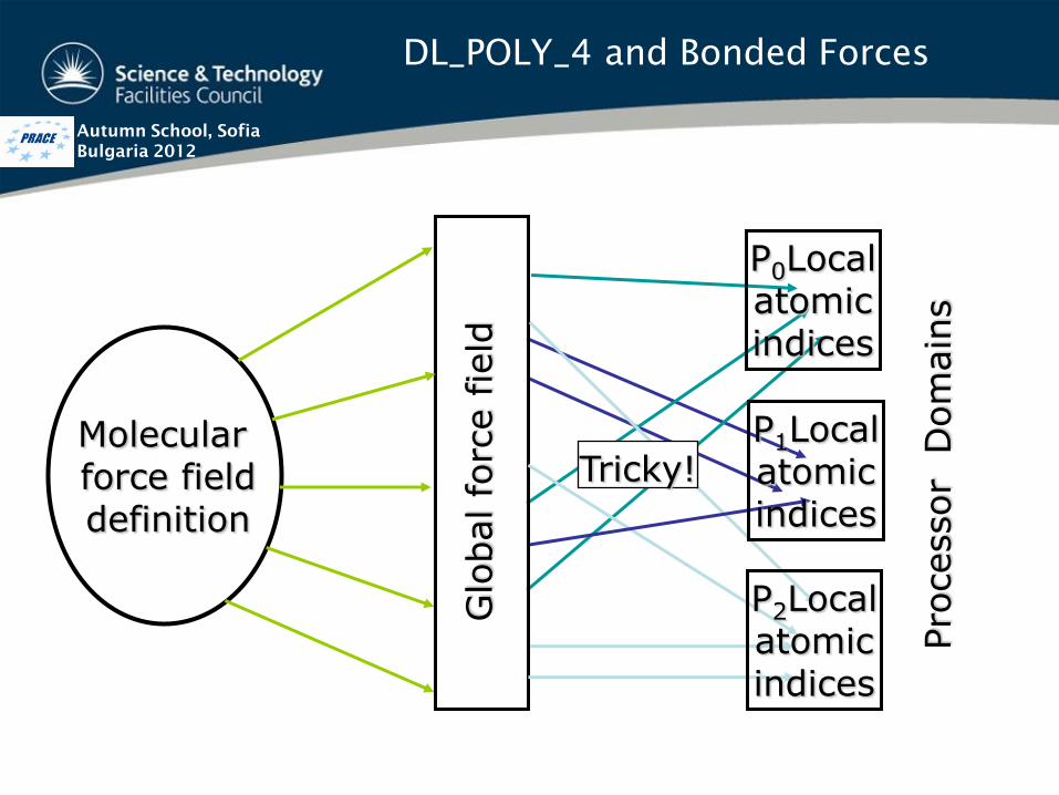
Bulgaria 2012
Glo
bal fo
rce f
ield
P0Local atomic indices
P1Local atomic indices
P2Local atomic indices
Pro
cessor
Dom
ain
s
Tricky! Molecular force field definition
DL_POLY_4 and Bonded Forces

Autumn School, Sofia
Bulgaria 2012
Ensembles and Algorithms
Integration:
Available as velocity Verlet (VV) or leapfrog Verlet (LFV)
generating flavours of the following ensembles
• NVE
• NVT (Ekin
) Evans
• NVT Andersen^, Langevin^, Berendsen, Nosé-Hoover, GST
• NPT Langevin^, Berendsen, Nosé-Hoover, Martyna-
Tuckerman-Klein^
• NT/NPnAT/NPnT Langevin^, Berendsen, Nosé-Hoover,
Martyna-Tuckerman-Klein^
Constraints & Rigid Body Solvers:
• VV dependent – RATTLE, No_Squish, QSHAKE*
• LFV dependent – SHAKE, Euler-Quaternion, QSHAKE*

Autumn School, Sofia
Bulgaria 2012
Integration Algorithms
Essential Requirements:
• Computational speed
• Low memory demand
• Accuracy
• Stability (energy conservation, no drift)
• Useful property - time reversibility
• Extremely useful property – symplecticness
= time reversibility + long term stability

Autumn School, Sofia
Bulgaria 2012
r (t)
r (t+t) v (t)t
f(t)t2/m
r’ (t+t)
[r (t), v(t), f(t)] [r (t+t), v(t+t), f(t+t)]
Integration: Essential Idea

Autumn School, Sofia
Bulgaria 2012
Simulation Cycle and Integration Schemes
Setup
Forces
Motion
Stats.
Results
Set up initial
system
Calculate
forces
Calculate
motion
Accumulate
statistical data
Summarise
simulation
Taylor expansion:
)()()(.3
)()()(.2
)(.1
)(),(.0
21
21
21
21
ttvttxttx
m
tftttvttv
afreshcalculatedtf
ttvtx
iii
i
iii
i
ii
Leapfrog Verlet (LFV) Velocity Verlet (VV)
i
iii
i
iii
i
iii
iii
m
ttftttvttv
afreshcalculatedttf
ttvt
txttx
m
tfttvttv
tftvtx
)(
2)()(.VV2.1
)(.0VV2.
)(2
)()(.2VV1.
)(
2)()(.1VV1.
)(),(),(.0VV1.
21
21
21
32
12
tOm
ftvtrr n
nnn

Autumn School, Sofia
Bulgaria 2012
Integration Algorithms: Leapfrog Verlet
Discrete time
rn+1 rn rn-1 rn-2
vn+1/2
f n f n-1 f n-2
vn-1/2 vn-3/2
)(
)(
42/11
32/12/1
tvtrr
tFm
tvv
n
i
n
i
n
i
n
i
i
n
i
n
i
Application in Practice
2
2/12/1
2/11
2/12/1
n
i
n
in
i
n
i
n
i
n
i
n
i
i
n
i
n
i
vvv
vtrr
Fm
tvv

Autumn School, Sofia
Bulgaria 2012
Integration Algorithms: Velocity Verlet
Discrete time
rn+1 rn rn-1 rn-2
vn+1 vn vn-1 vn-2
f n+1 f n f n-1 f n-2
12/11
2/11
2/1
2
2
n
i
i
n
i
n
i
n
i
n
i
n
i
n
i
i
n
i
n
i
Fm
tvv
vtrr
Fm
tvv
Application in Practice
)()(2
)(2
211
42
1
tFFm
tvv
tFm
tvtrr
n
i
n
i
i
n
i
n
i
n
i
i
n
i
n
i
n
i

Autumn School, Sofia
Bulgaria 2012
Constraint Solvers
SHAKE
RATTLE
RATTLE_R (SHAKE)
Taylor expansions:
32
12
tOm
gftvtrr nn
nnn
3
122
1 tOm
hftvv nn
nn
jiij
u
ij
o
ij
u
ijijij
ij
o
ijijjiij
mm
dd
dd
tg
dgGG
111
)(
2
22
2
u
ij
o
ij
u
ij
o
ijij
ijdd
dd
tg
)(22
2
RATTLE_V
ijd
i
j
o
iv
o
iv
2
)(
ij
o
ijjiij
ij
o
ijijjiij
d
dvv
th
dhHH
o
ijd
ijd
u
ijd
oioj
ui i
ujj
jiG
ijG

Autumn School, Sofia
Bulgaria 2012
Extended Ensembles in VV casting
Velocity Verlet integration algorithms can be naturally derived from the
non-commutable Liouvile evolution operator by using a second order
Suzuki-Trotter expansion. Thus they are symplectic/true ensembles
(with conserved quantities) warranting conservation of the phase-space
volume, time-reversibility and long term numerical stability…
Examplary VV Expansion of NVE to NVEkin
, NVT, NPT & NσT
ttttRRATTLE
tttvt
txttx
tm
tfttvttv
tttttThermostat
ttttBarostat
ttttThermostat
tftvtx
iii
i
iii
iii
:)(_
:)(2
)()(
:)(
2)()(
:)(
:)(
:)(
)(),(),(
:VV1
21
21
21
41
21
41
21
21
41
41
tttttThermostat
tttttBarostat
tttttThermostat
tttttVRATTLE
tm
ttftttvttv
afreshttfttvttx
i
iii
iii
41
23
21
21
41
43
21
21
21
21
21
:)(
:)(
:)(
:)(_
:)(
2)()(
)(),(),(
:VV2

Autumn School, Sofia
Bulgaria 2012
Other Integration Algorithms
• Gear Predictor-Corrector – generally easily
extendable to any high order of accuracy.
It is used in satellite trajectory
calculations/corrections. However, lacking
long term stability.
• Trotter derived evolution algorithms –
generally easily extendable to any high
order of accuracy. Symplectic.

Autumn School, Sofia
Bulgaria 2012
Base Functionality
• Molecular dynamics of polyatomic systems with
options to save the micro evolution trajectory at
regular intervals
• Optimisation by conjugate gradients method or zero
Kelvin annealing
• Statistics of common thermodynamic properties
(temperature, pressure, energy, enthalpy, volume)
with options to specify collection intervals and stack
size for production of rolling and final averages
• Calculation of RDFs and Z-density profiles
• Temperature scaling, velocity re-Gaussing
• Force capping in equilibration
Autumn School, Sofia
Bulgaria 2012
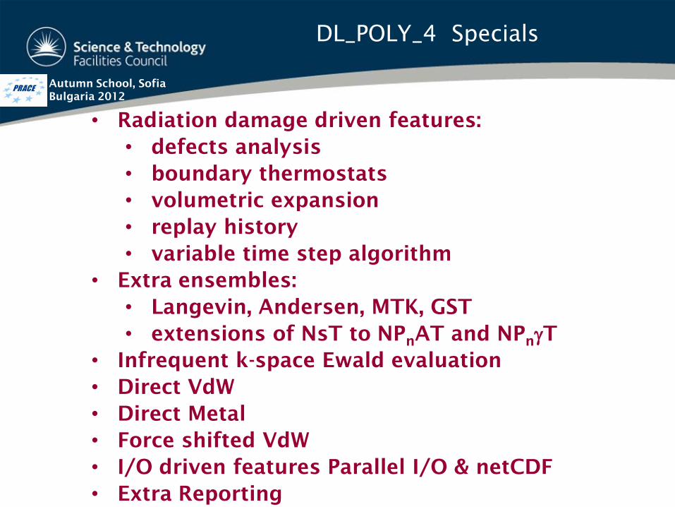
• Radiation damage driven features:
• defects analysis
• boundary thermostats
• volumetric expansion
• replay history
• variable time step algorithm
• Extra ensembles:
• Langevin, Andersen, MTK, GST
• extensions of NsT to NPnAT and NP
nT
• Infrequent k-space Ewald evaluation
• Direct VdW
• Direct Metal
• Force shifted VdW
• I/O driven features Parallel I/O & netCDF
• Extra Reporting
DL_POLY_4 Specials

Autumn School, Sofia
Bulgaria 2012
Part 3
DL_POLY I/O Files

Autumn School, Sofia
Bulgaria 2012
I/O Files
• Crystallographic
(Dynamic) data
• Simulation
Control data
• Molecular /
Topological Data
• Tabulated two-
body potentials
• EAM potential
data
• Reference data
for DEFECTS
• Restart data
• Final
configuration
• Simulation
summary data
• Trajectory Data
• Defects data
• MSD & T inst
data
• Statistics data
• Best CGM
configuration
• RDF data
• Z density data
• Restart data

Autumn School, Sofia
Bulgaria 2012
Internally, DL_POLY uses atomic scale units:
• Mass - mass of H atom (D) [Daltons]
• Charge - charge on proton (e)
• Length - Angstroms (Å)
• Time - picoseconds (ps)
• Force - D Å ps-2
• Energy - D Å2 ps
-2 [10 J mol
-1]
pressure is expressed in k-atm for I/O
DL_POLY Units

Autumn School, Sofia
Bulgaria 2012
UNITS directive in FIELD file allows to opt for the
following energy units
• Internal DL_POLY units - 10 J mol-1
• Electron-volts - eV
• Kilo calories per mol - k-cal mol-1
• Kilo Joules per mol - k-J mol-1
• Kelvin per Boltzmann - K Boltzmann-1
All interaction MUST have the same energy units!
Acceptable DL_POLY Units

Autumn School, Sofia
Bulgaria 2012
• SIMULATION CONTROL
• Free Format
• Mandatory
• Driven by keywords:
keyword [options] {data}
e.g.:
ensemble NPT Hoover 1.0 8.0
CONTROL File

Autumn School, Sofia
Bulgaria 2012
CONFIG [REVCON,CFGMIN] File
• Initial atomic coordinates
• Format
- Integers (I10)
- Reals (F20)
- Names (A8)
• Mandatory
• Units:
- Position - Angstroms (Å)
- Velocity – Å ps-1
- Force - D Å ps-2
• Construction:
- Some kind of GUI essential
for complex systems

Autumn School, Sofia
Bulgaria 2012
• Force Field specification
• Mandatory
• Format:
- Integers (I5)
- Reals (F12)
- Names (A8)
- Keywords (A4)
• Maps on to CONFIG file
structure
• Construction
- Small systems - by hand
- Large systems – nfold or
GUI!
FIELD File

Autumn School, Sofia
Bulgaria 2012
• Defines non-analytic
pair (vdw) potentials
• Format
- Integers (I10)
- Reals (F15)
- Names (A8)
• Conditional, activated
by FIELD file option
• Potential & Force
• NB force (here) is:
)()( rUr
rrG
TABLE File

Autumn School, Sofia
Bulgaria 2012
• Defines embedded atom potentials
• Format
- Integers (I10)
- Reals (F15)
- Names (A8)
• Conditional, activated by FIELD file option
• Potentials only
• pair, embed & dens keywords for atom types
followed by data records (4 real numbers per
record)
• Individual interpolation arrays
TABEAM File

Autumn School, Sofia
Bulgaria 2012
• Provides program restart capability
• File is unformatted (not human readable)
• Contains thermodynamic accumulators, RDF
data, MSD data and other checkpoint data
• REVIVE (output file) ---> REVOLD (input file)
REVOLD [REVIVE] File

Autumn School, Sofia
Bulgaria 2012
• Provides Job Summary (mandatory!)
• Formatted to be human readable
• Contents:
- Summary of input data
- Instantaneous thermodynamic data at selected intervals
- Rolling averages of thermodynamic data
- Statistical averages
- Final configuration
- Radial distribution data
- Estimated mean-square displacements and 3D diffusion
coefficient
• Plus:
- Timing data, CFG and relaxed shell model iteration data
- Warning & Error reports
OUTPUT File

Autumn School, Sofia
Bulgaria 2012
• System properties at
intervals selected by user
• Optional
• Formatted (I10,E14)
• Intended use: statistical
analysis (e.g. error) and
plotting vs. time.
• Recommend use with GUI!
• Header:
- Title
- Units
• Data:
- Time step, time, #
entries
- System data
STATIS File

Autumn School, Sofia
Bulgaria 2012
Configuration data at user
selected intervals
• Formatted
• Optional
Header:
• Title
• Data level, cell key, number
Configuration data:
• Time step and data keys
• Cell Matrix
• Atom name, mass, charge
• X,Y,Z coordinates (level 0)
• X,Y,Z velocities (level 1)
• X,Y,Z forces (level 2)
HISTORY File

Autumn School, Sofia
Bulgaria 2012
• Formatted (A8,I10,E14)
• Plotable
• Optional
• RDFs from pair forces
• Header:
- Title
- No. plots & length of plot
• RDF data:
- Atom symbols (2)
- Radius (A) & RDF
- Repeated……
• ZDNDAT file has same format
RDFDAT [ZDNDAT] File

Autumn School, Sofia
Bulgaria 2012
• REFERENCE file
– Reference structure to compare against
• DEFECTS file
– Trajectory file of vacancies and interstitials
migration
• MSDTMP file
– Trajectory like file containing the each particle’s
Sqrt(MSDmean
) and Tmean
DL_POLY_4 Extra Files

Autumn School, Sofia
Bulgaria 2012
Part 5
DL_POLY_4 Performance

Autumn School, Sofia
Bulgaria 2012
Proof of Concept on IBM p575 2005
300,763,000 NaCl with full SPME electrostatics
evaluation on 1024 CPU cores
Start-up time 1 hour
Timestep time 68 seconds
FFT evaluation 55 seconds
In theory ,the system can be seen by the eye. Although
you would need a very good microscope – the MD cell
size for this system is 2μm along the side and as the
wavelength of the visible light is 0.5μm so it should be
theoretically possible.

Autumn School, Sofia
Bulgaria 2012
2000 4000 6000 8000 10000 12000 14000 16000
2000
4000
6000
8000
10000
12000
14000
16000
14.6 million particle Gd2Zr
2O
7 system
Sp
ee
d G
ain
Processor count
Perfect
MD step total
Link cells
van der Waals
Ewald real
Ewald k-space
Benchmarking BG/L Jülich 2007

Autumn School, Sofia
Bulgaria 2012
0 200 400 600 800 1000
0
200
400
600
800
1000
max load 700'000 atoms per 1GB/CPU
max load 220'000 ions per 1GB/CPU
max load 210'000 ions per 1GB/CPU
Solid Ar (32'000 atoms per CPU)
NaCl (27'000 ions per CPU)
SPC Water (20'736 ions per CPU)
21 million atoms
28 million atoms
33 million atoms
good parallelisation
perfect p
aralle
lisatio
n
Sp
ee
d G
ain
Processor Count
DL_POLY_4 Weak Scaling

Autumn School, Sofia
Bulgaria 2012
0
1
2
3
4
5
6
7
8
9
10
0 100 200 300 400 500 600
ste
ps
pe
r se
con
d
Np
Scaling
ICE7
ICE7_CB
DL_POLY_4 RB v/s CB
on 450,000 particles

Autumn School, Sofia
Bulgaria 2012
Benchmarking Main Platforms
0 500 1000 1500 2000
0
1
2
3
4
5
6
7
8
9
3.8 million particle Gd2Zr
2O
7 system
Eva
lua
tion
s [s
-1]
Processor count
CRAY XT4 SC
CRAY XT4 DC
CRAY XT3 SC
CRAY XT3 DC
BG/L
BG/P
IBM p575
3GHz Woodcrest DC

Autumn School, Sofia
Bulgaria 2012
I/O Solutions in DL_POLY_4
1. Serial read and write (sorted/unsorted) – where only a single
MPI task, the master, handles it all and all the rest communicate in
turn to or get broadcasted to while the master completes writing a
configuration of the time evolution.
2. Parallel write via direct access or MPI-I/O (sorted/unsorted) –
where ALL / SOME MPI tasks print in the same file in some orderly
manner so (no overlapping occurs using Fortran direct access
printing. However, it should be noted that the behaviour of this
method is not defined by the Fortran standard, and in particular we
have experienced problems when disk cache is not coherent with the
memory).
3. Parallel read via MPI-I/O or Fortran
4. Serial NetCDF read and write using NetCDF libraries for
machine-independent data formats of array-based, scientific data
(widely used by various scientific communities).

Autumn School, Sofia
Bulgaria 2012
3.09 3.10 3.09 3.10
Cores I/O Procs Time/s Time/s Mbyte/s Mbyte/s
32 32 143.30 1.27 0.44 49.78
64 64 48.99 0.49 1.29 128.46
128 128 39.59 0.53 1.59 118.11
256 128 68.08 0.43 0.93 147.71
512 256 113.97 1.33 0.55 47.60
1024 256 112.79 1.20 0.56 52.47
2048 512 135.97 0.95 0.46 66.39
MPI-I/O Write Performance for
216,000 Ions of NaCl on XT5

Autumn School, Sofia
Bulgaria 2012
3.10 New 3.10 New
Cores I/O Procs Time/s Time/s Mbyte/s Mbyte/s
32 16 3.71 0.29 17.01 219.76
64 16 3.65 0.30 17.28 211.65
128 32 3.56 0.22 17.74 290.65
256 32 3.71 0.30 16.98 213.08
512 64 3.60 0.48 17.53 130.31
1024 64 3.64 0.71 17.32 88.96
2048 128 3.75 1.28 16.84 49.31
MPI-I/O Read Performance for
216,000 Ions of NaCl on XT5
Autumn School, Sofia
Bulgaria 2012
Part 4
Obtaining & Building DL_POLY

Autumn School, Sofia
Bulgaria 2012
DL_POLY Licensing and Support
• Online Licence Facility at http://www.ccp5.ac.uk/DL_POLY/
• The licence is
• To protect copyright of Daresbury Laboratory
• To reserve commercial rights
• To provide documentary evidence justifying continued
support by UK Research Councils
• It covers only the DL_POLY_4 package
• Registered users are entered on the DL_POLY e-mailing list
• Support is available (under CCP5 and EPSRC service level
agreement to CSED) only to UK academic researchers
• For the rest of the world there is the online user forum
• Last but not least there is a detailed, interactive, self-
referencing PDF (LaTeX) user manual

Autumn School, Sofia
Bulgaria 2012
• Register at http://www.ccp5.ac.uk/DL_POLY/
• Registration provides the decryption - procedure
and password (sent by e-mail)
• Source is supplied by anonymous FTP (in an
invisible directory)
• Source is in a tarred, gzipped and encrypted form
• Successful unpacking produces a unix directory
structure
• Test and benchmarking data are also available
Supply of DL_POLY_4

Autumn School, Sofia
Bulgaria 2012
DL_POLY_Classic Support
• Full documentation of software supplied with source
• Support is available through the online user forum or
the CCP5 user community
WWW:
http://www.ccp5.ac.uk/DL_POLY_CLASSIC/
FTP:
ftp://ftp.dl.ac.uk/ccp5/DL_POLY/
FORUM:
http://www.cse.stfc.ac.uk/disco/forums/ubbthreads.php/

Autumn School, Sofia
Bulgaria 2012
• Downloads are available from CCPForge at
http://ccpforge.cse.rl.ac.uk/gf/project/dl_poly_classic/
• No registration required – BSD licence
• Download source from: CCPForge: Projects: DL_POLY
Classic: Files: dl_poly_classic: dl_poly_classic1.9
• Sources is a in tarred and gzipped form
• Successful unpacking produces a unix directory
structure
• Test data are also available
Supply of DL_POLY_Classic

Autumn School, Sofia
Bulgaria 2012
DL_POLY
build
source
execute
java
utility
Home of makefiles
DL_POLY source code
Home of executable & Working Directory
Java GUI source code
Utility codes
data Test data
DL_POLY Directory Structure

Autumn School, Sofia
Bulgaria 2012
• Read README.txt file in source and follow
instructions within
• Copy Makefile from `build’ to`source’
• Use `make machinetype’ to compile e.g
make gfortran
• Executable in `execute’ directory
• DLPOLY.X is DL_POLY_Classic executable
• DLPOLY.Z is DL_POLY_4 executable
• Standard executables have been made
available on many architectures
Compiling the DL_POLY code

Autumn School, Sofia
Bulgaria 2012
1. Note differences in capabilities (e.g. linked rigid bodies) !!!
2. Less than 10,000 atoms (if in parallel)? – DL_POLY Classic
3. More than 30,000 atoms? – DL_POLY_4
4. Ratio cell_width/rcut
< 3 (in any direction)? – DL_POLY_Classic
5. Less than 500 particles per processor? – DL_POLY_Classic
DL_POLY_C versus DL_POLY_4
for parallel jobs
DL_POLY_Classic
Simple molecules (no SHAKE)
• 8 or less, 10,000 atoms
• 16 or less, 20,000 atoms
• 32 or less, 30,000 atoms
Simple ionics
• 16 or less, 10,000 atoms
• 64 or less, 20,000 atoms
• 128 or less, 30,000 atoms
Molecules (with SHAKE)
• 64 max!
DL_POLY_4
• Golden Rule 1: No fewer than
3x3x3 link cells per processor (if
in parallel)
• Golden Rule 2: No fewer than
500 particles per processor (if in
parallel)!

Autumn School, Sofia
Bulgaria 2012
Part 6
DL_POLY_Classic Functionality W. Smith

Autumn School, Sofia
Bulgaria 2012
Special Algorithms
• Hyperdynamics
– Bias potential dynamics
– Temperature accelerated dynamics
– Nudged elastic band
• Solvation properties:
– Energy decomposition
– Spectroscopic solvent shifts
– Free energy of solution
• Metadynamics

Autumn School, Sofia
Bulgaria 2012
Standard Input Special Input Standard Output Special Output
CONFIG REVOLD OUTPUT HISTORY
FIELD TABLE STATIS RDFDAT
CONTROL TABEAM REVIVE ZDNDAT
REVCON
HYPOLD HYPRES
EVENTS
CFGBSNnn
CFGTRAnn
PROnn.XY
SOLVAT
FREENG
STEINHARDT METADYNAMICS
ZETA
CFGMIN
Operation Type:
Standard use
Hyperdyn./TAD
Solvation
Hyperdynamics
Optimisation
I/O Files

Autumn School, Sofia
Bulgaria 2012
Solvation Features
• Molecular Solvation Energy
• Energy decomposition
• Energy distribution functions
• Free Energy of Solvation
• Mixed Hamiltonian method
• Thermodynamic Integration
• Solution Spectroscopy
• Solvent induced shifts
• Solvation relaxation

Autumn School, Sofia
Bulgaria 2012
• SOLVAT
– Breakdown of system energy based on
molecular types
– Energies of ground and excited states
• FREENG
– Energy data for thermodynamic integration
Solvation Files

Autumn School, Sofia
Bulgaria 2012
Bias Potential Dynamics
Temperature Accelerated Dynamics
Metadynamics
Hyperdynamics

Autumn School, Sofia
Bulgaria 2012
• Construct bias potential
to reduce well depth of
state A.
• Bias potential is zero at
saddle point.
• Ratios of rates from state
A to states B, C, etc.
preserved:
• Suitable bias potential:
Bias Potential Dynamics
Original
Potential
Bias
Potential
Modified
Potential
State A

Autumn School, Sofia
Bulgaria 2012
Bias Potential Dynamics 2
b
b
bb
bb
b
b
A
N
b
A
TSTTST
*
bA
N
bA
NTST
A
N
bA
N
bNTST
ANTST
A
N
b
A
N
b
N
A
NN
b
N
b
N
NN
b
N
b
NN
A
NN
NNN
A
RVkk
RVRVRVk
RVRVRVk
RVk
RV
RVff
dRVRVH
dRVRVHff
dH
dHff
exp/or
0 if exp/ and
exp/exp So
Now
exp
exp
exp
exp
exp
exp
*
*
*

Autumn School, Sofia
Bulgaria 2012
Temperature Accelerated Dynamics
First order reactions:
Hopping probability:
P dt = k exp(-kt) dt
Lifetime of state: =1/k
Arrhenius:
k = A exp(-E*/RT)
log(1/) = log A - E*/RT 1/RTh 1/RTl 1/RToo
log
(1/)
p1
p2
E1
E2
increasing
simulation
time
stop time tend

Autumn School, Sofia
Bulgaria 2012
Temperature Accelerated Dynamics 2
• Simulate system at high T & watch for transitions
• When transition found, stop simulation and:
– Determine activation energy using nudged elastic
band
– Record transition time, save `new’ state
configuration
• Restart simulation in original state with new velocities.
• Search for new transitions. Hence build `library’ of
transition data.
• Stop searching after time tend
given by:
tend
=exp[E2+(T
h-T
l)(E
2-)/T
h]
• Commence new search from `first’ low T state.

Autumn School, Sofia
Bulgaria 2012
Nudged Elastic Band
A
B
E
R
A B
C1 CN-1
C2 C3 C4
C0 CN
• N+1 configs (C0…CN) linearly
interpolated From A to B
• Connect by spring (stiffness K)
• Remove `off tangent’ forces
• Minimise all configs subject to
presence of spring forces
• Resulting path is reaction path
through saddle point

Autumn School, Sofia
Bulgaria 2012
Kinetic Monte Carlo
• Simulate set of competing processes
• Rate of process is (make a list).
• Define sum of rates
• Generate random number
• Select process
• Advance time
• Repeat!
Nipi ,,1;
ipir
N
i
irR1
10 : uu
i
j
j
i
j
ji ruRrp1
1
1
:
R
uRip
Rut /)log(
Autumn School, Sofia
Bulgaria 2012
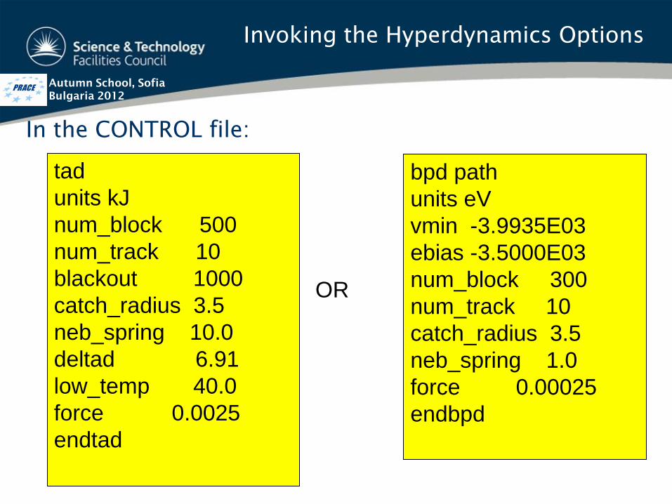
Invoking the Hyperdynamics Options
In the CONTROL file:
tad
units kJ
num_block 500
num_track 10
blackout 1000
catch_radius 3.5
neb_spring 10.0
deltad 6.91
low_temp 40.0
force 0.0025
endtad
bpd path
units eV
vmin -3.9935E03
ebias -3.5000E03
num_block 300
num_track 10
catch_radius 3.5
neb_spring 1.0
force 0.00025
endbpd
OR

Autumn School, Sofia
Bulgaria 2012
Additional files for TAD and Bias potential
dynamics:
• HYPRES/HYPOLD – restart files
• EVENTS –program activity report
• CFGBSNnn – Basin CONFIG files (new states)
• PROnn.XY – Reaction path profiles
• CFGTRAnn – Tracking CONFIG files
Subdirectories required in execute directory:
BASINS, PROFILES, TRACKS
Hyperdynamics Files

Autumn School, Sofia
Bulgaria 2012
TAD – DL_POLY Test Case 32
• Atoms `hop’ into vacancies
• Each vacancy has 12 nearest neighbour
atoms
• So 12 possible escapes from PE basin
• Use TAD to find them!
• Use NEB to find activation energy
• Extrapolate to low temperature for low
T rate
• Put results into KMC simulation
255 L-J Argon atoms FCC crystal + 1 vacancy
EVENTS file extract:
Event nt Basins Nt E Time(ps) Extrap.(ps) Stop time(ps)
TRA 38500 0 1 1 7.28338E+00 3.82250E+01 4.31244E+07 2.04398E+03
TRA 55500 0 2 1 7.20808E+00 5.49650E+01 5.36891E+07 2.04398E+03
TRA 127500 0 3 1 7.28160E+00 1.26145E+02 1.41830E+08 2.04398E+03
TRA 750500 0 4 1 7.19597E+00 7.47515E+02 7.13444E+08 2.04398E+03

Autumn School, Sofia
Bulgaria 2012
BPD – DL_POLY Test Case 33
998 NaCl ions rocksalt crystal + 2 vacancies
Event nt Basins Nt E Time(ps) Extrap.(ps)
TRA 4500 0 1 1 6.74301E-01 4.39500E+00 7.34793E+03
TRA 399300 1 2 1 1.11127E+00 3.99185E+02 6.45155E+05
TRA 466500 2 3 1 6.57466E-01 4.66495E+02 7.53837E+05
EVENTS file extract:
• Overall neutral system
• Ions `hop’ into vacancies
• Escapes from PE basin unknown (a
priori)
• Use BPD to find them!
• Use NEB to find activation energy
• Extrapolate hopping time for zero
bias
• Put results into KMC simulation

Autumn School, Sofia
Bulgaria 2012
NEB Reaction Profiles
Lennard Jones Argon
Sodium Chloride

Autumn School, Sofia
Bulgaria 2012
Metadynamics
Metadynamics is a method devised by Alessandro Laio
and Michele Parrinello for accelerating the exploration
of a free energy landscape as the function of collective
variables.
Method:
• The system potential energy is augmented by a time-
dependent bias potential consisting of Gaussian
functions of the collective variables
• The longer a simulation remains in a particular free
energy minimum, the larger the bias potential becomes
– thus forcing the system to seek out a new
thermodynamic state.
• The accumulated bias potential provides a description
of the free energy surface

Autumn School, Sofia
Bulgaria 2012
Metadynamics in 1D
A. Laio & M. Parrinello, PNAS 99 (2002) 12562

Autumn School, Sofia
Bulgaria 2012
Collective Variables?
A collective variable is a single number that defines
an atomic structure (i.e. it is a function of ). Most often
they are called Order Parameters. Particular examples
used in metadynamics are:
• The system potential energy:
• Simulation cell vectors:
• The Steinhardt order parameters:
• Tetrahedral order parameters:
and are maximum for particular structures.
Defining the bias potential in terms of order parameters
allows destabilization of particular structural phases.
)(N
rU
Q
Nr
Q
),,( cbah

Autumn School, Sofia
Bulgaria 2012
Metadynamics Formulae
Order parameter vector:
System Hamiltonian:
Bias Potential:
and are chosen to `fill’ surface at acceptable rate
Force:
Free Energy Surface:
)(,),()( 1
N
M
NNMrsrsrs
]),([)(21
2
trsVrUm
pH
NMNN
i i
i
gN
k
M
k
MnMhtssWtrsV
1
22
2/)()(exp]),([
)()(1
N
ji
M
j j
N
iirs
s
VrUf
]),([lim
)( trsVt
sFNMM
g
W h

Autumn School, Sofia
Bulgaria 2012
• METADYNAMICS
– Data defining the metadynamics hypersurface
• STEINHARDT
– Defines the Steinhardt order parameters
• ZETA
– Defines the tetrahedral order parameters
Metadynamics Files

Autumn School, Sofia
Bulgaria 2012
Steinhardt Order Parameters
if 0
if 1)(
)(cos
2
1
if 1
)(
and and typesatom connecting vectors allover runs where
,)(
with, and typesatomfor
1
12
4
2
21
12
1
1
1
2/12
rr
rrrrr
rr
rr
rf
Nb
YrfQ
QNN
Q
c
b
bbmb
N
b
cm
m
m
C
b

Autumn School, Sofia
Bulgaria 2012
) typeof are atoms all (assuming atom
tolinked atoms of pairs ofnumber theis and
species of atoms allover run ,, Where
)3/1)(cos()(1
1
2
c
N
i
N
ij
N
jk
jikikcijc
c
N
Nkji
rfrfNN
T
Tetrahedral Order Parameters

Autumn School, Sofia
Bulgaria 2012
Ice Nucleation and Growth 1
0.5ns
D Quigley and PM Rodger, Molec. Sim. 35 (2009) 613
Bias:
Q4
OO, Q
6
OO, T
& PE

Autumn School, Sofia
Bulgaria 2012
Ice Nucleation and Growth 2
0.75ns
D Quigley and PM Rodger, Molec. Sim. 35 (2009) 613
Bias:
Q4
OO, Q
6
OO, T
& PE

Autumn School, Sofia
Bulgaria 2012
Ice Nucleation and Growth 3
1.25ns
D Quigley and PM Rodger, Molec. Sim. 35 (2009) 613
Bias:
Q4
OO, Q
6
OO, T
& PE

Autumn School, Sofia
Bulgaria 2012
Ice Nucleation and Growth 4
1.5ns
D Quigley and PM Rodger, Molec. Sim. 35 (2009) 613
Bias:
Q4
OO, Q
6
OO, T
& PE

Autumn School, Sofia
Bulgaria 2012
Conclusions
• DL_POLY Classic is free
• It's very versatile with advanced features
• Go get it!

Autumn School, Sofia
Bulgaria 2012
Part 7
The DL_POLY Java GUI W. Smith

Autumn School, Sofia
Bulgaria 2012
• Java - Free!
• Facilitate use of code
• Selection of options (control of capability)
• Construct (model) input files
• Control of job submission
• Analysis of output
• Portable and easily extended by user
GUI Overview

Autumn School, Sofia
Bulgaria 2012
• Edit source in java directory
• Edit using vi,emacs, whatever
• Compile in java directory:
javac *.java
jar -cfm GUI.jar manifesto *.class
• Executable is GUI.jar
• But.....
****Don't Panic!****
The GUI.jar file is provided in the download
Compiling/Editing the GUI

Autumn School, Sofia
Bulgaria 2012
• Invoke the GUI from within the execute directory (or
equivalent):
java -jar ../java/GUI.jar
• Colour scheme options:
java -jar ../java/GUI.jar –colourscheme
with colourscheme one of:
monet, vangoch, picasso, cezanne, mondrian (default
picasso).
Invoking the GUI

Autumn School, Sofia
Bulgaria 2012
Menus
The Monitor Window

Autumn School, Sofia
Bulgaria 2012
Using Menus
Show Editor Option

Autumn School, Sofia
Bulgaria 2012
Graphics Buttons
The Molecular Viewer
Graphics Window
Editor Button

Autumn School, Sofia
Bulgaria 2012
Editor Buttons
The Molecular Editor
Editor Window

Autumn School, Sofia
Bulgaria 2012
• File - Simple file manipulation, exit etc.
• FileMaker - make input files:
– CONTROL, FIELD, CONFIG, TABLE
• Execute
– Select/store input files, run job
• Analysis
– Static, dynamic,statistics,viewing,plotting
• Information
– Licence, Force Field files, disclaimers etc.
Available Menus

Autumn School, Sofia
Bulgaria 2012
Buttons
Text Boxes
A Typical GUI Panel

Autumn School, Sofia
Bulgaria 2012
• VMD is a free software package for visualising MD
data.
• Website: http://www.ks.uiuc.edu/Research/vmd/
• Useful for viewing snapshots and movies.
– A plug in is available for DL_POLY HISTORY files
– Otherwise convert HISTORY to XYZ or PDB format
DL_POLY & VMD

Autumn School, Sofia
Bulgaria 2012
This will consist of (up to) five components:
• A demonstration of the Java GUI
• Download & compile DL_POLY classic
• Trying some DL_POLY simulations:
– prepared exercises, or
– creative play
• DL_POLY clinic - what’s up doc?
• Group therapy – all for one and one for all
....
“Hands-On Session”

Autumn School, Sofia
Bulgaria 2012
Part 9
DL_FIELD C.W. Yong

Autumn School, Sofia
Bulgaria 2012
xyz
PDB
DL_FIELD
‘black box’ FIELD CONFIG
DL_FIELD
• AMBER & CHARM to DL_POLY Input Format
• OPLS-AA & Drieding to DL_POLY Input Format
Protonated

Autumn School, Sofia
Bulgaria 2012
• VMD is a free software package for visualising MD data
• Website: http://www.ks.uiuc.edu/Research/vmd/
• Useful for viewing snapshots and movies.
– A plug in is available for DL_POLY HISTORY files
– Otherwise convert HISTORY to XYZ or PDB format
DL_POLY & VMD

Autumn School, Sofia
Bulgaria 2012
Part 10
DL_MESO M. Seaton

Autumn School, Sofia
Bulgaria 2012
Part 11
DL_POLY Hands-On
http://www.ccp5.ac.uk/DL_POLY/TUTORIAL/EXERCISES/index.html

Autumn School, Sofia
Bulgaria 2012
UV
k
kq ik rc
o kj j
j
N
1
2
42 2
20 1
2
exp( / )exp
1
4
4
0
3 2
2
1
o
n j
jnn j
N
Rjn
o
jj
N
q q
R rerfc R r
q
/
k
Vm n 2
1 3
/
( , , )with:
The Ewald Summation

Autumn School, Sofia
Bulgaria 2012
2
10
2
22
exp)4/exp(
2
1
N
j
jj
ko
recip rkiqk
k
VU
The crucial part of the SPME method is the conversion
of the Reciprocal Space component of the Ewald sum
into a form suitable for Fast Fourier Transforms (FFT).
Thus:
),,(),,(2
1321
,,
321
321
kkkQkkkGV
Ukkk
T
o
recip
becomes:
where G and Q are 3D grid arrays (see later)
Ref: Essmann et al., J. Chem. Phys. (1995) 103 8577
Smoothed Particle-Mesh Ewald

Autumn School, Sofia
Bulgaria 2012
Central idea - share discrete charges on 3D grid:
Cardinal B-Splines Mn(u) - in 1D:
)1(1
)(1
)(
)0,max()!(!
!)1(
)!1(
1)(
/2exp)1()/)1(2exp()(
/2exp)()(/2exp
11
1
0
12
0
uMn
unuM
n
uuM
kuknk
n
nuM
KikMKknikb
KikuMkbLkiu
nnn
nn
k
k
n
n
n
jnj
Recursion
relation
SPME: Spline Scheme

Autumn School, Sofia
Bulgaria 2012
321 ,,
333322221111
1
321
)()()(
),,(
nnn
jnjnjn
N
j
j KnuMKnuMKnuMq
Q
GT (k1,k2,k3) is the discrete Fourier Transform of the
function:
*
3213212
22
321 )),,()(,,()4/exp(
),,( kkkQkkkBk
kkkkG T
2
33
2
22
2
11321 )()()(),,( kbkbkbkkkB with
Is the charge array and QT(k1,k2,k3) its discrete Fourier transform.
SPME: Building the Arrays

Autumn School, Sofia
Bulgaria 2012
• SPME is generally faster then conventional Ewald sum in
most applications. Algorithm scales as O(NlogN)
• In DL_POLY_Classic the FFT array is built in pieces on
each processor and made whole by a global sum for the FFT
operation
• In DL_POLY_4 the FFT array is built in pieces on each
processor and kept that way for the distributed FFT
operation (DaFT)
• The DaFT FFT `hides’ all the implicit communications
SPME: Comments

Autumn School, Sofia
Bulgaria 2012
FFTs are
• Fast (!) - O(VlogV) operations where V is the number of
points in the grid
• Global operations - to perform a FFT you need all the
points
• This makes it difficult to write an efficient, good scaling
FFT
Parallel FFTs - The Basics

Autumn School, Sofia
Bulgaria 2012
• Distribute the data by planes
• Each processor has a complete set of points in the x and y
directions so can do those Fourier transforms
• Redistribute data so that a processor holds all the points in z
• Do the z transforms
• Allows efficient implementation of the serial FFTs ( use a
library routine )
• In practice for large enough 3D FFTs can scale reasonably
• However, the distribution does not map onto DL_POLY’s -
large amounts of data redistribution
Traditional Parallel FFTs

Autumn School, Sofia
Bulgaria 2012
• Takes data distributed as in DL_POLY_4 (Domain
Decomposition) thus avoiding a lot of communication in
comparison to traditional 3D FFT routines (due to data
redistribution) when used on more than 8-64 CPUs
• So do a distributed data FFT in the x direction then the y
and finally the z directions
• Disadvantage is that can not use the library routine for the
1D FFT ( not quite true … )
• Scales quite well - e.g. on 512 procs, an 8x8x8 CPU grid, a
1D FFT need only scale to 8 CPU
• Totally avoids data redistribution, exists as a stand alone
F90 library.
Daresbury advanced Fourier Transforms

Autumn School, Sofia
Bulgaria 2012
U. Essmann, L. Perera, M.L. Berkowtz, T. Darden, H. Lee, L.G.
Pedersen, J. Chem. Phys., (1995), 103, 8577
1. Calculate self interaction correction
2. Initialise FFT routine (FFT – 3D FFT)
3. Calculate B-spline coefficients
4. Convert atomic coordinates to scaled fractional units
5. Construct B-splines
6. Construct charge array Q
7. Calculate FFT of Q array
8. Construct array G
9. Calculate FFT of G array
10. Calculate net Coulombic energy
11. Calculate atomic forces
RD Scheme for long-ranged part of SPME

Autumn School, Sofia
Bulgaria 2012
U. Essmann, L. Perera, M.L. Berkowtz, T. Darden, H. Lee, L.G.
Pedersen, J. Chem. Phys., 103, 8577 (1995)
1. Calculate self interaction correction
2. Initialise FFT routine (FFT – IJB’s DaFT: 3M2 1D FFT)
3. Calculate B-spline coefficients
4. Convert atomic coordinates to scaled fractional units
5. Construct B-splines
6. Construct partial charge array Q
7. Calculate FFT of Q array
8. Construct partial array G
9. Calculate FFT of G array
10. Calculate net Coulombic energy
11. Calculate atomic forces
I.J. Bush, I.T. Todorov, W. Smith, Comp. Phys. Commun., 175, 323
(2006)
DD Scheme for long-ranged part of SPME

Autumn School, Sofia
Bulgaria 2012
Simplest option:
ewald precision [] (tolerance)
Advanced option (for anisotropic systems,
particularly with slabs):
ewald [] [kmax1
] [kmax2
] [kmax3
]
with
= exp[-( rcut
)2]/r
cut (solve for )
= exp[-(km
/2)2]k
m
2 (solve for k
m)
kmax n
=Lnk
m/2 , where L
n is the MD box width in
n direction
Choosing Ewald Sum Parameters