Ⓔ

Distance and Azimuthal Dependence of Ground-Motion

Variability for Unilateral Strike-Slip Ruptures

by Jagdish Chandra Vyas, Paul Martin Mai, and Martin Galis

Abstract We investigate near-field ground-motion variability by computing theseismic wavefield for five kinematic unilateral-rupture models of the 1992 Mw 7.3Landers earthquake, eight simplified unilateral-rupture models based on the Landersevent, and a large Mw 7.8 ShakeOut scenario. We include the geometrical fault com-plexity and consider different 1D velocity–density profiles for the Landers simulationsand a 3D heterogeneous Earth structure for the ShakeOut scenario. For the Landersearthquake, the computed waveforms are validated using strong-motion recordings.We analyze the simulated ground-motion data set in terms of distance and azimuthdependence of peak ground velocity (PGV).

Our simulations reveal that intraevent ground-motion variability ϕln�PGV� is higherin close distances to the fault (<20 km) and decreases with increasing distance fol-lowing a power law. This finding is in stark contrast to constant sigma-values used inempirical ground-motion prediction equations. The physical explanation of a largenear-field ϕln�PGV� is the presence of strong directivity and rupture complexity. Highvalues of ϕln�PGV� occur in the rupture-propagation direction, but small values occur inthe direction perpendicular to it. We observe that the power-law decay of ϕln�PGV� isprimarily controlled by slip heterogeneity. In addition, ϕln�PGV�, as function ofazimuth, is sensitive to variations in both rupture speed and slip heterogeneity. Theazimuth dependence of the ground-motion mean μln�PGV� is well described by aCauchy–Lorentz function that provides a novel empirical quantification to modelthe spatial dependency of ground motion.

Online Material: Figures of slip distributions, residuals to ground-motion predic-tion equations (GMPEs), distance and azimuthal dependence, and directivity predictorof ground-motion variability for different source models.

Introduction

Seismic-hazard analysis generally involves usingground-motion prediction equations (GMPEs), derived fromstrong-motion recordings, to estimate ground-shaking levelsfor future earthquakes. The GMPEs relate predictor variablesY such as peak ground velocity (PGV), peak ground accel-eration (PGA), and pseudospectral acceleration (PSA) toexplanatory variables such as earthquake magnitude, source-to-site distance, faulting style, and site class (e.g., Akkar andBommer, 2007a,b; Abrahamson and Silva, 2008; Boore andAtkinson, 2008; Chiou and Youngs, 2008; Bindi et al.,2014). Ground motions computed using GMPEs are given interms of the natural logarithm of the median Y (μln�Y�) and itsstandard deviation (ϕln�Y�), typically referred to as ground-motion variability.

Ground-motion variability associated with ground-motion prediction results from incomplete data sets andimperfect modeling, that is, lack of knowledge (epistemic

uncertainty) or uncertainty due to nature’s randomness (alea-tory variability). There are attempts to separate and quantifyepistemic and aleatoric components of ϕln�Y� (Anderson andBrune, 1999; Atkinson, 2013), but here we assume that ϕln�Y�represents only aleatoric ground-motion variability (Booreand Atkinson, 2008; Campbell and Bozorgnia, 2008). ϕln�Y�can be further subdivided into an intraevent component (i.e.,for a single event considering all records at the same source-to-site distance) and an interevent component (i.e., at a singlereceiver considering all events).

Strasser et al. (2009) summarized the problems andchallenges when estimating ϕln�Y�. Among these, the lack ofnear-field recordings in strong-motion data sets is perhapsthe most important one. Also, the available data are biased:many recordings exist for a few earthquakes, whereas only afew strong-motion data were recorded for many events (inparticular for earthquakes that occurred before 1994). It is

BSSA Early Edition / 1

Bulletin of the Seismological Society of America, Vol. 106, No. 4, pp. –, August 2016, doi: 10.1785/0120150298

important to note that ϕln�Y� controls the shape of the seismic-hazard curve, in particular for long return periods, and thushas significant impact on probabilistic seismic-hazard analy-sis (e.g., Bommer and Abrahamson, 2006). Therefore, it is ofparamount importance to understand and precisely quantifythe sources of ground-motion variability to improve ground-motion prediction for future earthquakes.

GMPEs are commonly specified using constant ϕln�Y�(e.g., Boore et al., 1997; Chiou and Youngs, 2006; Booreand Atkinson, 2008). Some of the more recent GMPEs haveincorporated earthquake-magnitude dependence of ϕln�Y�(e.g., Abrahamson and Silva, 2008; Chiou and Youngs,2008). ϕln�Y� has also been analyzed as a function of source-to-site distance and rupture style. The most recent GMPE ofBoore et al. (2014) includes a distance dependence of ϕln�Y�,which is constant up to a Joyner–Boore distance (RJB) of100 km, followed by a slight increase due to regional varia-tions in anelastic attenuation. Investigating the JapaneseKiK-net strong-motion catalog, Rodriguez-Marek et al.(2011) observed that ϕln�Y� not only depends on earthquakemagnitude, but also on source-to-site distance. They also dis-covered that the correlation of ϕln�Y� with magnitude anddistance is not consistent across different spectral periods.Imtiaz et al. (2015) found that the intraevent ϕln�Y� alsoshows distance dependence with rupture style: for bilateralruptures, ϕln�Y� tends to increase with distance, whereasfor unilateral ruptures, ϕln�Y� tends to decrease with distance.Youngs et al. (1995) reported that ϕln�Y� decreases withincreasing magnitude and that the magnitude dependenceis stronger for the interevent ϕln�Y� than for the intraeventϕln�Y�. In summary, ground-motion variability has beenfound to depend on earthquake magnitude, rupture style, dis-tance, and azimuth. However, the corresponding number ofstudies is limited, whereas the governing physics of potentialϕln�Y� dependencies is not yet fully understood.

In general, ground motion and its variability are deter-mined by source, path, and site effects (e.g., Mai, 2009).However, the lack of near-field recordings hampers thedevelopment of a complete understanding of the physicalcauses of ground-motion variability. Therefore, physics-based simulation techniques that include a specified but com-plex rupture processes and wave-propagation effects are usedto compute and analyze near-field ground motion and itsvariability (e.g., Spudich and Frazer, 1984; Komatitsch andTromp, 1999; Dumbser and Kaeser, 2006; Mai et al., 2010).Ripperger et al. (2008) showed that the azimuthal depend-ence of interevent ground-motion variability is strongest inthe backward-directivity region. Imperatori and Mai (2012)quantified how ground-motion variability is influenced bythe level of heterogeneity in several earthquake source mod-els, as well as by different 1D models of Earth structure. Thesource-induced ground-motion variability is important atshort-to-intermediate periods (<2 s) but negligible at longperiods, whereas ground-motion variability associated withcrustal models becomes significant at intermediate-to-longperiods (>0:5 s). Recently, Ramirez-Guzman et al. (2015)

performed numerical simulations for the 1811–1812 NewMadrid earthquakes, demonstrating that ground-motion vari-ability is strongly affected by basin and rupture directivityeffects. Mena and Mai (2011) employed kinematic rupturemodels to investigate the effect of source complexity on thenear-field velocity pulses to quantify the directivity effect.They found that directivity pulses are primarily related to slipheterogeneity (i.e., the size and location of slip asperities).

In the present study, we perform numerical simulations tofurther investigate the influence of the earthquake ruptureprocess on near-field ground-motion variability, addressingthe directivity effects in particular. Henry and Das (2001)showed that both strike-slip and dip-slip earthquakes tend tobe unilateral, as indicated by the average hypocenter locationwithin 25% of the fault length from the nearest end of the fault.McGuire et al. (2002) found that approximately 80% of alllarge earthquakes (Mw >7) are predominantly unilateral.Mai et al. (2005) investigated the location of hypocenter po-sitions along-strike and down-dip directions from invertedearthquake source models for small-to-large earthquakes.They found that small earthquakes (Mw <6) tend to rupturein the center of the fault plane, which can be due to thelimited resolution of finite-source inversions for the smallearthquakes. However, they observed that moderate-to-largeearthquakes tend to nucleate towards one end of the fault, rup-turing to the other end unilaterally (particularly strike-slipearthquakes). The unilateral character of large strike-slipearthquakes suggests that their near-field ground motions maycontain a strong directivity effect. In such cases, the unilateralrupture propagation, combined with the S-wave radiation pat-tern, produces strong shaking in the region of the forward-rupture-propagation direction. We conjecture that this maylead to higher near-field ground-motion variability comparedto bilateral ruptures. Therefore, we consider earthquakes withstrong unilateral rupture propagation to investigate near-fieldground-motion variability as a function of distance and azi-muth. We attempt to gain a deeper physical understanding ofground-motion variability, but we do not provide any correc-tion terms to existing GMPEs (e.g., Spudich and Chiou, 2008).

In our ground-motion simulations, we use kinematic rup-ture models in which the rupture process is specified byassigning the spatiotemporal evolution of slip on the faultin terms of local slip-velocity functions and the rupture veloc-ity. The rupture models are chosen such that comparison withobservations allows us to validate our simulations and developa new ϕln�Y� parameterization that we then test against a largescenario event. We choose the 1992 Mw 7.3 Landers earth-quake, which is characterized by unilateral rupture propaga-tion with strong directivity effect (e.g., Somerville et al.,1997). As the large scenario event, we use one of theMw 7.8 ShakeOut unilateral ruptures on the San Andreas fault(Graves et al., 2008). For both events, we simulate the seismicwavefield at a large number of sites and analyze correspond-ing PGV values. We restrict ourselves to PGV because the sim-ulations would become prohibitively expensive for the higherfrequencies needed to study PGA, which also would require

2 J. C. Vyas, P. M. Mai, and M. Galis

BSSA Early Edition

inclusion of seismic-scattering effects that may lead to de-creasing directivity signature (e.g., Boatwright, 2007; Seekinsand Boatwright, 2010; Imperatori and Mai, 2013). For ournumerical simulations, we use a generalized finite-differencecode based on a support operator method (SORD code by Elyet al., 2008), which is second-order accurate in space and timeand naturally handles geometrically complex kinematic sourcemodels embedded in 3D Earth structure.

The subsequent sections are organized as follows. First,we describe our approach to ground-motion simulations fortheMw 7.3 Landers earthquake and perform statistical analy-sis on the computed shaking levels. We then present our re-sults on the observed spatial dependencies of ϕln�Y� andinvestigate the rupture parameters that control ϕln�Y� of low-frequency ground motions. Finally, we analyze the ground-motion simulations from a large Mw 7.8 ShakeOut scenarioto validate our findings from the Landers earthquake.

Ground-Motion Simulations for the 1992 Mw 7.3Landers Earthquake

In this section, we introduce the kinematic rupturemodels of the Mw 7.3 Landers earthquake and proposed 1Dvelocity–density structures, along with our source–receivergeometry to study ground-motion variability. We also sta-tistically compare our synthetics with observed strong-motion data to validate our numerical simulations.

Kinematic Source Models

From the Earthquake SourceModel Database (SRCMOD,Mai and Thingbaijam, 2014), we choose five published finite-fault kinematic rupture models inverted by five different re-search groups: (1) Cotton and Campillo (1995), (2) Hernandezet al. (1999), (3) Zeng and Anderson (2000), (4) Wald andHeaton (1994), and (5) Cohee and Beroza (1994). Subse-quently, we refer to each of these rupture models by the nameof the respective first author.

Table 1 lists certain inversion parameters used by thesefive groups: inversion method, type of data sets, frequencyrange, number of segments, and type of source time function.

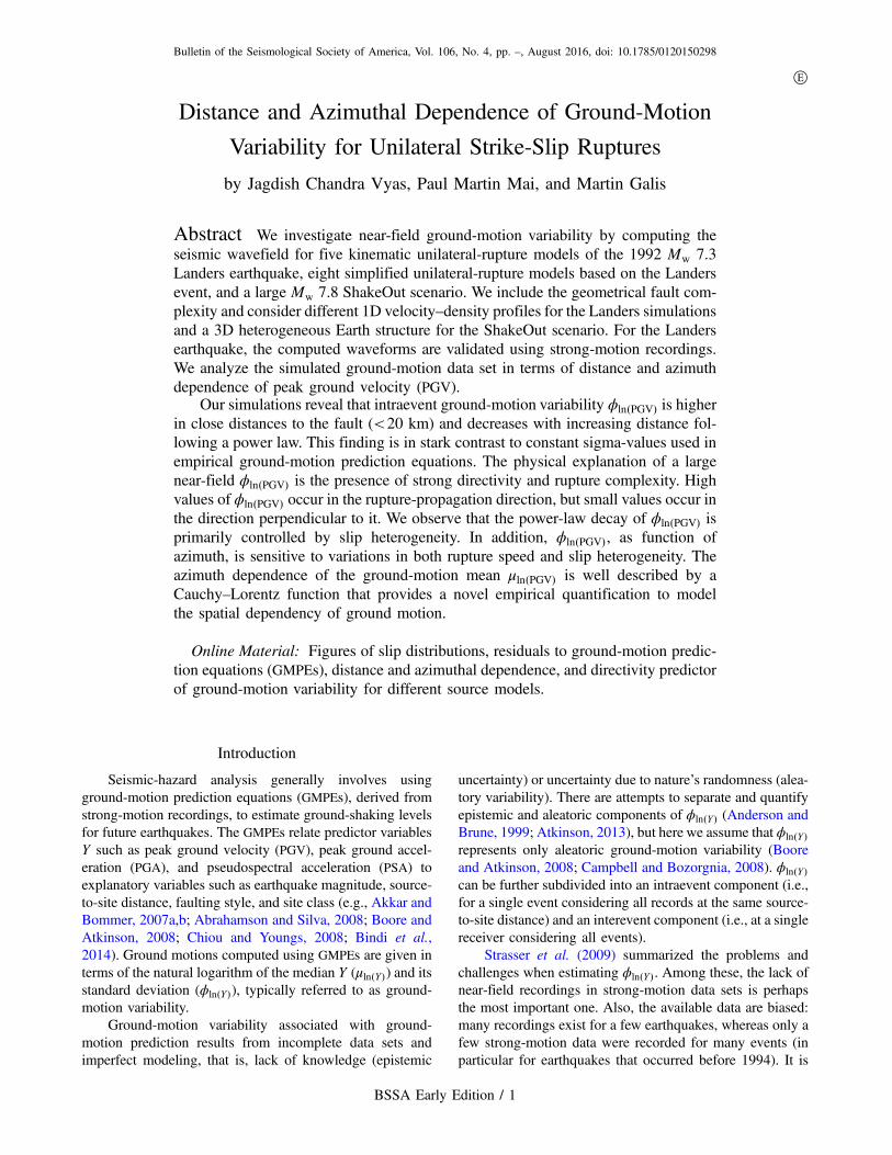
Figure 1 shows the bicubicly interpolated slip distributions ofthe five rupture models (the original slip distributions are dis-played in Ⓔ Fig. S1, available in the electronic supplementto this article), illustrating variations in the assumed faultgeometry among these models with respect to strike direc-tions and overlapping or nonoverlapping segments. We inter-polate the coarse inverted source models onto a finer grid toensure a smooth seismic wavefield. The total seismic mo-ment is conserved by rescaling interpolated slip values. Thegrid size of the inverted models varies between 0.5 and 5 km,whereas, for the interpolated sources, it ranges between 0.5and 0.6 km.

Cotton Hernandez

Zeng Wald

−30−20

−100

0

20

40

60

0

10

EW (km)

Cohee

NS (km)

Dep

th (

km) Slip (m)

0

2

4

6

8

Figure 1. Bicubicly interpolated slip distributions of the fivekinematic sources of the 1992 Landers earthquake used for thenumerical modeling. Red stars denote the hypocenter location. Co-ordinates are given in east–west (EW) direction and north–south(NS) direction with respect to the epicenter as origin of a Cartesiancoordinate system. Color-coded slip is in meters.

Table 1Source Parameters Used for Inversion by Five Different Groups

Parameter*Cotton and Campillo

(1995)Hernandez et al.

(1999)Wald and Heaton

(1994)Cohee and Beroza

(1994)Zeng and Anderson

(2000)

Frequency range (Hz) 0.05–0.5 0.05–0.5 0.077–0.5 0.05–0.25 0.13–1.43Data sets SGM SGM, GPS, InSAR SGM, Tele, GPS SGM SGMSTF Tanh Tanh Triangular Triangular CompositeNTW 1 1 6 1 1NSEG 3 3 3 3 5Inversion method Frequency domain

inversionFrequency domain

inversionDamped, linear

least-squaresinversion

Newton–Rephsoniterative inversion

Genetic algorithm

SGM, strong ground motion; GPS, Global Positioning System; InSAR, Interferometric Synthetic Aperture Radar; and Tele, teleseismic.*STF, source time function; NTW, number of time windows; NSEG, number of segments.

Distance and Azimuthal Dependence of Ground-Motion Variability for Unilateral Strike-Slip Ruptures 3

BSSA Early Edition

Earth Structure and Attenuation

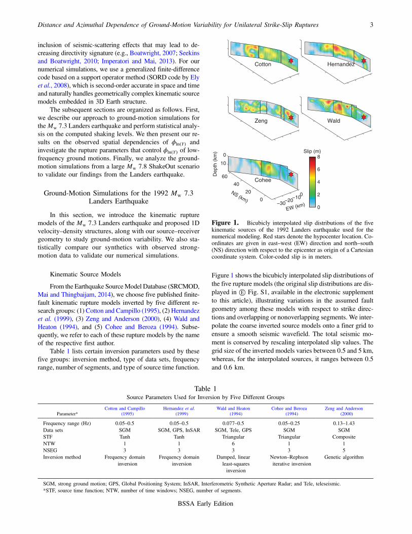
For our ground-motion simulations, we apply the same1D-layered Earth models as used in the corresponding inver-sion studies for the Cotton, Hernandez, Wald, and Coheesource models. For the Zeng source model, we adopt themedium parameters of Wald and Heaton (1994). Figure 2displays the corresponding depth distributions of seismic-wave speeds and density.

Because intrinsic attenuation is not implemented in theSORD code, we apply a Futterman filter based on thet�-operator that depends on travel time and Q-values (Varelaet al., 1993). The Cotton, Hernandez, and Wald models havebeen inverted considering depth-dependent Q. We obtain arepresentativeQ-value by calculating the weighted harmonicmean of Q for the three models, with weights assigned ac-cording to layer thicknesses. The representativeQ-values forZeng and Cohee models are adopted from the Wald model.The average Q-values then range from 216 to 481, depend-ing on the Earth structures used by different groups.

Receiver Configuration

To validate our simulations, we use recordings from 10stations of the California Strong Motion InstrumentationProgram (CSMIP) (Fig. 3, black triangles), obtained fromthe Consortium of Organizations for Strong Motion Obser-vation Systems (COSMOS) website (see Data and Resour-ces). For detailed statistical analysis, we consider a set of2500 receivers, randomly distributed to avoid any potentialspatial bias (Fig. 3, gray triangles). The station coordinates

are fixed with respect to the corresponding epicenter and areidentical for all considered rupture models. To avoid numeri-cal artifacts due to inaccurate point-source representation atvery small source–receiver distances, we do not include anystation with RJB less than 1 km. Therefore, the receivers usedfor our statistical analysis of ground-motion variabilityoccupy the RJB range from 1 to 106 km (Fig. 3).

Synthetic Seismograms and Validation

We restrict the maximum frequency in our simulationsto 0.5 Hz, consistent with the frequency range for which thekinematic models have been obtained (Table 1). Because theSORD code is second-order accurate in space and time, weparameterize the simulations with a minimum of 15 pointsper shortest wavelength to achieve accurate wave propaga-tion, leading to spatial grid sizes between 250 and 300 m(depending on the corresponding velocity model). The com-putational time step satisfies the numerical stability criteriagiven by Ely et al. (2008) and ranges from 0.015 to 0.020 s,depending on the particular velocity model.

For validation, we compare residuals of peak grounddisplacement (PGD) between our simulations and strong-motion observations, computed as res � ln�PGDobs=PGDsim�(Fig. 4a). All seismograms are band-pass filtered in the

2 3 4 5 6 7 80

5

10

15

20

25

30

35

40

Density (g/cm3) or Vs (km/s) or Vp (km/s)

Dep

th (

km)

Density Vs Vp

Cotton

Wald

Cohee

Figure 2. 1D velocity–density models used for the ground-mo-tion simulations of the 1992 Landers earthquake.

−100 −50 0 50 100

−100

−50

0

50

100

150

−180−165−150−135−120

−105

−90

−75

−60

−45

−30

−15

015 30

45

60

75

90

105

120

135

150

165180

AMB

BAR

DES

JOS

FRT

TWE

PALSIL INDHEM

EW (km)N

S (

km)

Figure 3. Source–receiver geometry in a Cartesian coordinatesystem centered on the epicenter. The red line represents the surfaceprojection of the fault geometry for the Cotton and Campillo (1995)source model. The black triangles depict 10 California Strong Mo-tion Instrumentation Program (CSMIP) strong-motion stations usedto validate the simulations. The gray triangles show receivers usedin the ground-motion variability investigation. The dashed blacklines mark azimuthal directions with respect to average strike (335°)and origin as epicenter.

4 J. C. Vyas, P. M. Mai, and M. Galis

BSSA Early Edition

0.05–0.5 Hz frequency range using a second-order Butter-worth filter. We determine PGD using the sensor-orientationindependent measure GMRotD50 (Boore et al., 2006), calcu-lated by rotating the two orthogonal horizontal componentsfrom 1° to 90° in steps of 1° and computing the geometricmean for each pair. The final PGD value is then given as themedian of 90 geometric means. We also calculate the residualmean and standard deviation for the 10 stations and for eachmodel (Fig. 4a), noting that most stations are located in thebackward-rupture-propagation direction. We find that oursimulations slightly underestimate PGD values, although thezero-residual line falls within the one standard deviation forall but the Cotton model. We note that the Zeng model yieldsthe lowest residuals, which we attribute to the fact that theZeng model was inverted using seismic data up to 1.4 Hz,whereas the remaining models use seismic waves only up to0.5 Hz, or even 0.25 Hz (Cohee model). Because our maintarget is investigating the spatial variability of ground motionsin a relative sense, but not in absolute amplitude, we considerthe level of agreement between synthetic and recorded wave-field as satisfactory.

In addition, we compare our simulations with a chosenGMPE by computing PGV from synthetic seismograms at2500 sites, again using the sensor-orientation independentmeasure GMRotD50. We then bin the PGV values withrespect to RJB (bin width � 20 km) and compute the natural-log-normal mean μln�PGV� and standard deviation ϕln�PGV� foreach bin. The bin width is chosen such that each bin containsat least 200 samples, whereas the mean RJB of all stationswithin any bin is near the center of the bin. We find thatthe simulation-based estimates of PGV fall within the twointraevent standard deviations of the selected GMPE (Booreand Atkinson, 2008) (Fig. 4b).

The above steps of validating our ground-motion simu-lation approach ensure that our subsequent analysis ofground-motion variability will not suffer from numericalartifacts or any unrealistic assumptions or parameter choices.

Analysis of Ground-Motion Variability

In this section, we analyze the ground-motion variabilityof PGV with respect to RJB and the source-to-site azimuthand compare PSA values from our simulations with GMPE-derived PSA estimates. We also consider an approach tocorrect ground-motion amplitudes with respect to directivitydue to the rupture-propagation directionality (Spudich andChiou, 2008).

Distance Dependence

For the analysis of ground-motion variability, we bin thePGV values at 2500 sites with respect to RJB distance using abin width of 20 km, with the constraint that each bin has atleast 200 stations. We also test the effect of bin width onϕln�PGV� by considering smaller (15 km) and larger (25 km)bin widths and find that all considered bin widths lead tosimilar results (compare Fig. 5 with Ⓔ Fig. S2a,b).

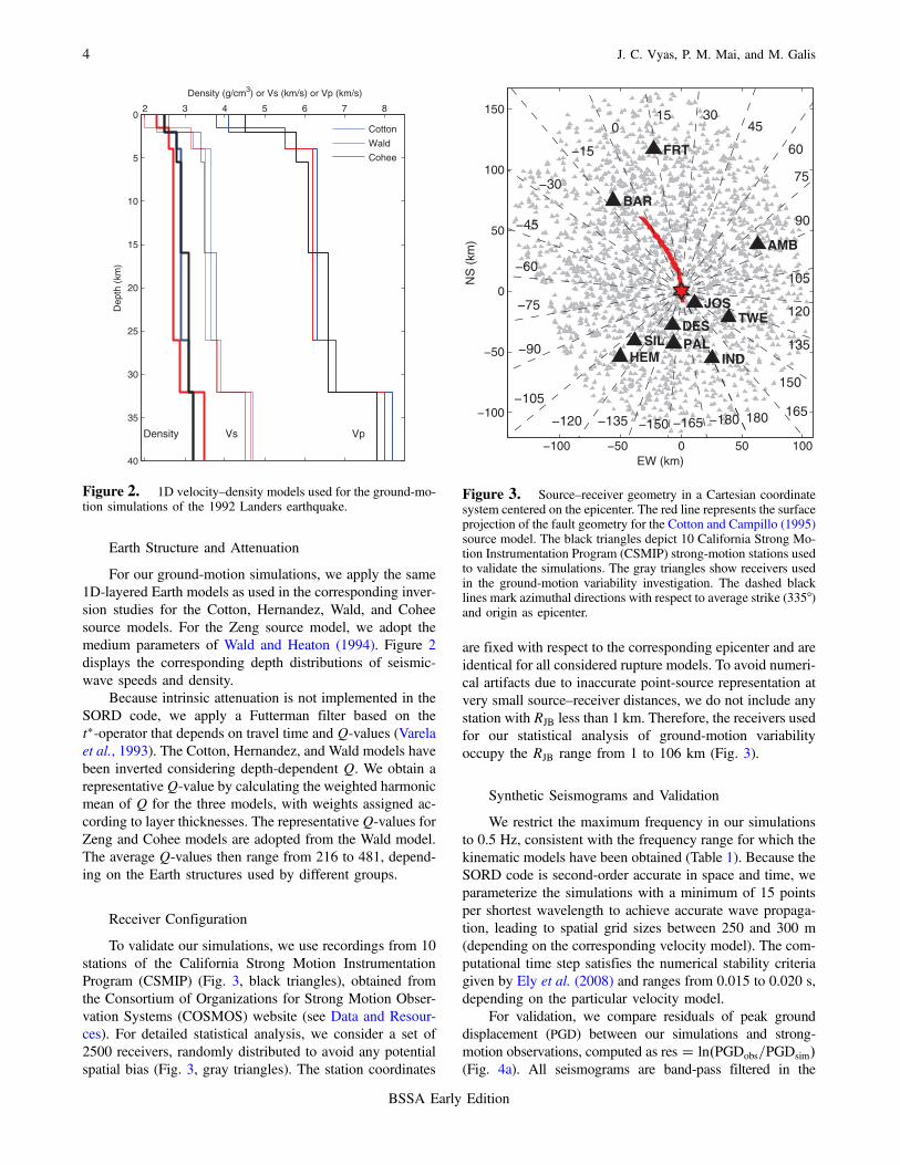
Figure 5 shows the distance dependence of the mean(μln�PGV�) and the standard deviation (ϕln�PGV�) of ln�PGV�.As expected, μln�PGV� decreases with increasing distance forall five models due to geometrical spreading and attenuation.For reference, we also display the intraevent ground-motionvariability from four GMPEs (Abrahamson and Silva, 2008;Boore and Atkinson, 2008; Campbell and Bozorgnia, 2008;Chiou and Youngs, 2008). We observe that ϕln�PGV� fromour simulations is higher in the very-near-field region(RJB < 20 km) than that estimated by GMPEs, but ϕln�PGV�decreases with increasing distance approaching the constantvalues of the GMPEs.

To examine the distance dependence of ground-motionvariability, we model the ϕln�PGV� dependence on RJB asa power law, ϕln�PGV� � αRk

JB. We estimate the values ofthe parameters α and k using least-square fitting (Table 2;corresponding curves are shown by dashed lines in Fig. 5).We also calculate the mean value of ϕln�PGV� and the power-

Cotton Hernandez Zeng Wald Cohee

−0.5

0

0.5

1

ln(P

GD

obs/P

GD

sim

)

(a)

101

102

100

101

RJB

(km)

PG

V (

cm/s

)

(b)

Cotton

Hernandez

Zeng

Wald

Cohee

BA GMPEBA 1&2 φ

ln(PGV)

Figure 4. (a) Statistical summary of peak ground displacement (PGD) residuals (in natural-log scale) between simulated and observedwaveforms for the five source models of the Landers earthquake. Different markers are used for different source models. The gray circlesshow the calculated mean residual, and gray bars show standard deviation for every source model. (b) Comparing mean and standarddeviation of peak ground velocity (PGV) computed from simulations with a ground motion prediction equation (GMPE) (Boore and Atkinson,2008). Different colored markers represent means of PGVs, and the bar indicates the corresponding standard deviation.

Distance and Azimuthal Dependence of Ground-Motion Variability for Unilateral Strike-Slip Ruptures 5

BSSA Early Edition

law fit for the ensemble (depicted by black circles and dashedlines in Fig. 5). We find α � 1:11 and k � −0:14 for themean ϕln�PGV�. For all cases considered, α is always positive,ranging between 0.82 and 1.47, whereas k is always nega-tive, ranging from −0:19 to −0:09. We find that the approxi-mation by a power law is applicable over the entire RJB rangeconsidered in this study (1 < RJB < 106 km), but we cannotassess whether this trend persists to larger distances.

The space–time complexity of the earthquake ruptureprocess has significant influence on near-field ground motionand its variability. In particular the directivity effect, due to acombination of the rupture-propagation direction and theS-wave radiation pattern, generates vastly different ground-motion amplitudes in the near field of large earthquakes, de-pending on whether the rupture propagates towards (forwarddirectivity) or away (backward directivity) from a site. TheLanders earthquake had strong directivity effect, as firstidentified by Somerville et al. (1997), resulting in higherground motion in the northern part of the fault because ofthe unidirectional (south-to-north) rupture propagation.The effect of geometrical spreading is the same for all sites

at a particular RJB distance and therefore does not affect theϕln�PGV� value for specific RJB distance. Consequently, geo-metrical spreading is not the cause for the distance decay ofϕln�PGV�, although it contributes to the distance decay ofμln�PGV�. On the other hand, the directivity effect is strongat near-source distances and becomes weaker farther awayfrom the source. Therefore, we interpret the distance decayof ϕln�PGV� as a consequence of the strong directivity effect.The power-law exponent k will be large (or small) in thepresence of strong (or weak) directivity. When the exponentk is zero, ϕln�PGV� is equal to α (i.e., ϕln�PGV� becomes con-stant), consistent with ground-motion variability of stan-dard GMPEs.

The five Landers source models considered here arederived by inversion of seismic and/or geodetic data. Ideally,they should predict identical ground motions. However, theuncertainties in kinematic inversions manifest themselves inintraevent ground-motion variability of the estimated ruptureparameters, which consequently contribute to predictedground motion and their variability (Fig. 5). Our results showthat the uncertainty of the inverted source models does notchange the power-law decay trend of ϕln�PGV�; however, itdoes affect the absolute values of ϕln�PGV�.

Azimuthal Dependence

Next, we analyze ground-motion variability as a func-tion of azimuth. Because the five rupture models have com-plex fault geometry, we compute azimuth with respect to theaverage strike direction and epicenter of each model. Theazimuth values range from 0° to 180° and from 0° to −180°,measured in clockwise and anticlockwise directions, respec-tively. The PGV values at the 2500 sites are then binned withrespect to azimuth to compute the mean (μln�PGV�) and thestandard deviation (ϕln�PGV�) of PGV, considering a lognor-mal distribution. We choose a bin width of 15° to ensure thateach bin has at least 30 stations, and we require that the meanazimuth lies near the center of the bin. To verify that ouranalysis does not depend on the bin width, we calculateμln�PGV� and ϕln�PGV� also for bin width 30° (compare Fig. 6with Ⓔ Fig. S3).

0.5

1

1.5

2

2.5

3

400 300 200

μ ln(

PG

V (

cm/s

) )

Cotton

Hernandez

Zeng

Wald

Cohee

101

102

0.5

0.6

0.7

0.8

0.9

1

RJB

(km)

φ ln(

PG

V (

cm/s

) )

α RJBk >> α = 1.11, k = −0.14

BA

CB

AS

CY

Figure 5. Distance dependence of the mean (μln�PGV�) and thestandard deviation (ϕln�PGV�) of ln�PGV� for the five source modelsof the Landers earthquake (bin width � 20 km). The circle size in-dicates the number of stations in each bin. The black circles are theaverage ϕln�PGV�. ϕln�PGV� decreases as a power law (αRk

JB) with in-creasing distance. The dashed line shows the least-squares fit to thecorresponding ϕln�PGV� values for different source models. Abbrevia-tions are as follows: BA, Boore and Atkinson (2008); CB, Campbelland Bozorgnia (2008); AS, Abrahamson and Silva (2008); and CY,Chiou and Youngs (2008).

Table 2Parameters α and k of the Power Law (αRk

JB) Obtained byLeast-Squares Fitting to the Distance Dependence of

ϕln�PGV� for the 1992 Landers Earthquake

Source Name α k

Cotton and Campillo (1995) 1.03 −0.13Hernandez et al. (1999) 0.82 −0.11Zeng and Anderson (2000) 0.96 −0.09Wald and Heaton (1994) 1.31 −0.19Cohee and Beroza (1994) 1.47 −0.18Average ϕln�PGV�* 1.11 −0.14

*PGV, peak ground velocity.

6 J. C. Vyas, P. M. Mai, and M. Galis

BSSA Early Edition

Figure 6 shows the azimuthal dependence of μln�PGV�and ϕln�PGV�. As expected, μln�PGV� is highest in the for-ward-directivity region (i.e., for average strike direction withazimuth 0°) and lowest in the backward-directivity region(i.e., for azimuth ±180°). This pattern reflects strong direc-tivity effects. We compute average μln�PGV� and find that it iswell described by a Cauchy–Lorentz function (Fig. 6) thathas its origin as a solution of a differential equation for forcedresonance and describes the shape of spectral lines in spec-troscopy. The unilateral rupture propagation with directivityeffect compresses the energy released in the forward direc-tion. The directivity-driven μln�PGV� pattern is analogous tospectral energy peaks, and therefore a Cauchy–Lorentz dis-tribution represents a directivity characterization based onfundamental wave physics. The functional form of this dis-tribution is given as

EQ-TARGET;temp:intralink-;df1;55;176y � Iγ2

�x − x0�2 � γ2� C; �1�

in which I, γ, and x0 are the height, the half-width at half-maximum, and the location parameter, respectively. C is theconstant translation term that shifts the level up and down. Asmall (large) γ indicates that the peak of the distribution issharp (broad), which implies strong (weak) directivity. Large(or small) values of I represent high (or low) PGV values in

forward directivity compared to the backward-directivity re-gion. If there is no directivity, then the pattern of μln�PGV� willsimply be a periodic function due to the S-wave radiationpattern, in which case the Cauchy–Lorentz distributioncannot be used. We estimate the corresponding coefficientsusing nonlinear optimization of fitting equation (1) to theaverage μln�PGV� (Fig. 6).

Analyzing the simulation results for all five rupturemodels, we find that ground-motion variability is high alongthe average strike direction (azimuth 0°). Smaller ground-motion variability occurs perpendicular to average strikedirection (azimuth� 90°), but it is high again along the−142:5° direction (Fig. 6). Any potential periodic pattern ofϕln�PGV� (due to the S-wave point-source radiation pattern) isdistorted due to the complexity of slip and rupture-propaga-tion effects. High ϕln�PGV� in the forward direction (azimuth0°) can be explained by location of fault segments with highslip patches in the forward direction; therefore, high andsmall values of PGV, and consequently higher ϕln�PGV�, arefound in the corresponding azimuthal bins. Also, unilateralrupture propagation compresses the radiated seismic energyin the forward direction, leading to further increase of PGVvalues in the bins in the forward direction. However, as theazimuth increases and sites are located farther away from theforward-rupture-propagation direction, the seismic wave en-ergy is more dispersed in time, while the distance from highslip patches increases. In combination, this leads to lowervariability of PGV values, and hence ϕln�PGV� is low alongazimuthal directions �90°. The azimuth angle −142:5°depicts the backward-rupture-propagation direction withrespect to the complex geometry of the fault (see Fig. 3).Hence, the high value of ϕln�PGV� along the −142:5° directionis, similarly as for the forward direction, a consequence ofthe directivity effect. In general, we find that ground-motionvariability is high in the forward- and backward-rupture-propagation direction but low in the perpendicular direction.Therefore, the distortion of the periodic pattern of ϕln�PGV� ismainly due to directivity. A detailed study on the influence ofrupture parameters on azimuthal variation of ϕln�PGV� will bepresented in the next section.

Comparison of Numerical Simulations withGMPE Estimates

We now compare our numerical results with GMPE es-timates to which we apply the directivity correction proposedby Spudich and Chiou (2008) derived for the GMPE byBoore and Atkinson (2008). Because the correction is appli-cable only to PSA, we compute PSA for natural periods at 5and 10 s with 5% damping ratio. The GMPE predicts thesame value of PSA (or PGV) for a given RJB in all directions(−180° to 180°). The directivity-corrected GMPE accountsfor rupture-propagation direction, and consequently PSAval-ues vary spatially even for a fixed RJB.

The directivity correction by Spudich and Chiou (2008)is based on the correction term fD:

0

0.5

1

1.5

2

2.5

3

150 100 50

I = 2.02 γ = 56.13 x

0 = 6.00

C = 0.45

μ ln(

PG

V (

cm/s

) )

Cotton

Hernandez

Zeng

Wald

Cohee

−180 −135 −90 −45 0 45 90 135 180

0.1

0.2

0.3

0.4

0.5

0.6

0.7

0.8

Azimuth from epicenter (°)

φ ln(

PG

V (

cm/s

) )

Figure 6. Azimuthal dependence of μln�PGV� and ϕln�PGV� for thefive source models (bin width � 15°). The circle size represents thenumber of stations in each bin. The black circles and line marksthe average μln�PGV� and average ϕln�PGV� for the five source models.The coefficients I, γ, x0, and C of the Lorentz function (black line)are obtained from nonlinear optimization for average μln�PGV�; 0°azimuth represents the average strike direction.

Distance and Azimuthal Dependence of Ground-Motion Variability for Unilateral Strike-Slip Ruptures 7

BSSA Early Edition

EQ-TARGET;temp:intralink-;df2;55;372fD � fr�Rrup�fM�Mw��a� b × IDP�; �2�

in which

EQ-TARGET;temp:intralink-;;55;336

fr � max�0;�1 −

max�0; Rrup − 40�30

��

and fM � min�1;max�0;Mw − 5:6�

0:4

�:

The factor fr denotes a distance taper that is unity for rupturedistances Rrup between 0 and 40 km and then tapers linearlyto zero at Rrup ≥ 70 km. fM is a magnitude taper that is zerofor the 0–5.6 earthquake magnitude (Mw) range and rises lin-early to unity at Mw ≥6:0. Equation (2) includes an iso-chrone directivity predictor (IDP) that Spudich and Chiou(2008) calculate using the isochrone velocity ratio and theradiation-pattern amplitude at a specific location (Spudichand Frazer, 1984), accounting for complex geometry andrupture-propagation direction.

For computing this directivity correction, the connectedsegmented geometries (with no overlap between segments)used in the Cotton, Hernandez, and Zeng models are consid-ered as a single-fault rupture from the definition of Spudichand Chiou (2008). The overlapping segments of the Waldand Cohee models are considered as multifault ruptures. Ac-

cordingly, each segment of these models has its own hypo-center location, assigned based on the rupture onset timedistributions. It should be noted that fD does not account forheterogeneity of slip and rupture speed, both of whichstrongly affect the radiation pattern and hence directivityeffect. Because the directivity correction is zero forRJB > 70 km, we compute fD for 1–71 km RJB range forall five source models at 5 and 10 s periods (Ⓔ Fig. S4).

At each station, we compare residuals R �ln�PSAsim=PSAGMPE� and RfD � ln�PSAsim=PSAGMPEfD

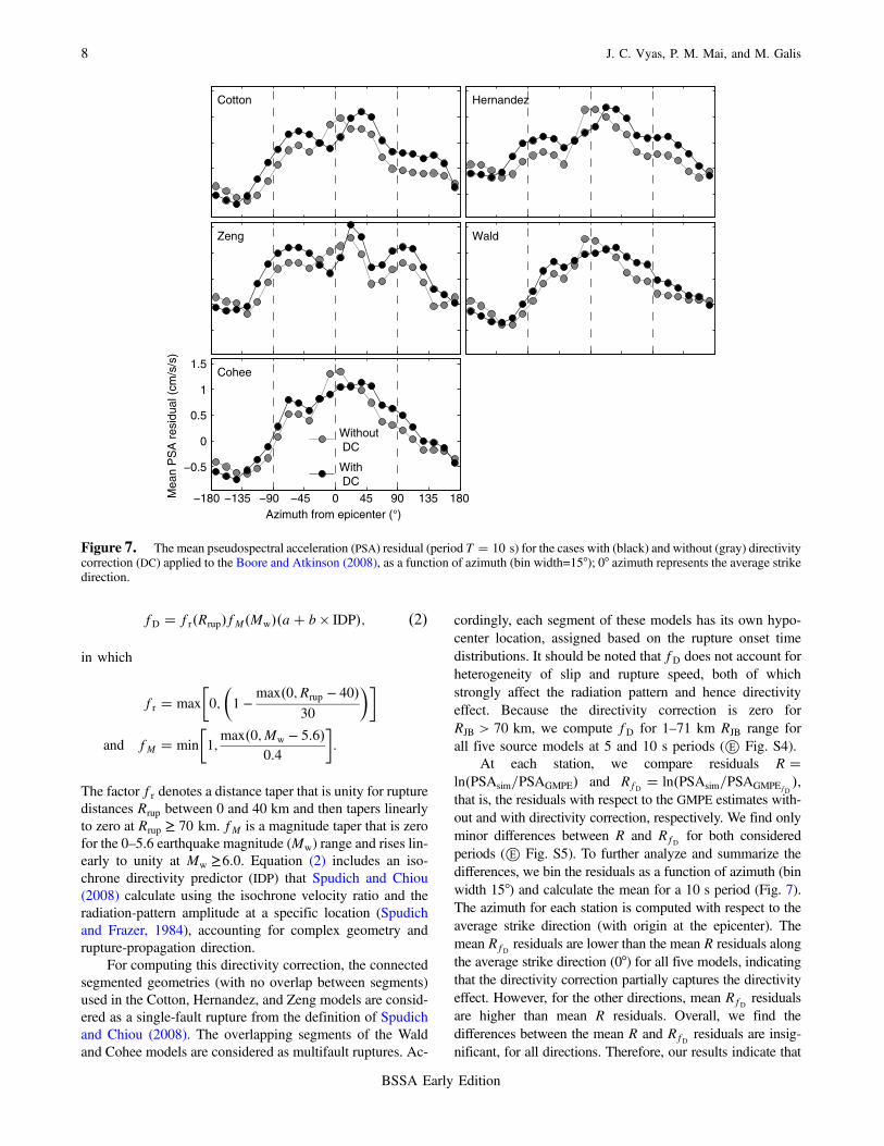
�,that is, the residuals with respect to the GMPE estimates with-out and with directivity correction, respectively. We find onlyminor differences between R and RfD for both consideredperiods (Ⓔ Fig. S5). To further analyze and summarize thedifferences, we bin the residuals as a function of azimuth (binwidth 15°) and calculate the mean for a 10 s period (Fig. 7).The azimuth for each station is computed with respect to theaverage strike direction (with origin at the epicenter). Themean RfD residuals are lower than the mean R residuals alongthe average strike direction (0°) for all five models, indicatingthat the directivity correction partially captures the directivityeffect. However, for the other directions, mean RfD residualsare higher than mean R residuals. Overall, we find thedifferences between the mean R and RfD residuals are insig-nificant, for all directions. Therefore, our results indicate that

Cotton Hernandez

Zeng Wald

−180 −135 −90 −45 0 45 90 135 180

−0.5

0

0.5

1

1.5Cohee

Azimuth from epicenter (°)

Mea

n P

SA

res

idua

l (cm

/s/s

)

Without DC

With DC

Figure 7. The mean pseudospectral acceleration (PSA) residual (period T � 10 s) for the cases with (black) and without (gray) directivitycorrection (DC) applied to the Boore and Atkinson (2008), as a function of azimuth (bin width=15°); 0° azimuth represents the average strikedirection.

8 J. C. Vyas, P. M. Mai, and M. Galis

BSSA Early Edition

the directivity correction proposed by Spudich and Chiou(2008) does not fully capture the spatial variations in ground-motion variability. The space–time complexity of the earth-quake rupture process is unlikely to be sufficiently describedby the IDP term. Directivity effects are averaged by GMPEsbecause they are derived statistically by combining recordingsfrom many different earthquakes. Likewise, a directivity cor-rection provides an approach to quantify the average, or gen-eralized, directivity behavior, which appears insufficient tocapture the directivity signature in simulated ground motionsfor Landers source models. We also investigated PSA residualsbetween estimates from observed data (from 10 stations) andthe predictions using Boore and Atkinson (2008) for the caseswith and without directivity correction. The analysis of ob-served data confirms our findings from simulations that theSpudich and Chiou (2008) directivity correction has only asmall effect and does not capture full directivity signaturein ground motions.

Insights on Ground-Motion Variability fromSource Heterogeneity

In this section, we investigate ground-motions arisingfrom simplified canonical models to better understand theorigins of ground-motion variability and to identify keyparameters controlling ϕln�PGV�.

Canonical Models

We generate seven simplified canonical rupture modelsbased on the Cotton model of the Landers earthquake. Ourobjective is to analyze how (or if) heterogeneous slip, risetime, and rupture speed affect ground-motion variability.The canonical models, obtained by combinations of hetero-geneous and uniform distributions of source parameters, aresummarized in Table 3. For example, HDTr − UVr denotes arupture model with heterogeneous (H) slip (D) and rise time(Tr) but uniform (U) rupture speed (Vr). Interchangeablywith this notation, we will also use the nomenclaturem1–m9 (see Table 3). The uniform parameters are obtained

by computing the spatial average of the correspondingheterogeneous source quantity, resulting in mean values ofslip, rise time, and rupture speed of 241.46 cm, 3.18 s, and2:83 km=s, respectively. Fault geometry and source timefunction remain unchanged. Furthermore, we consider apoint source with the same seismic moment of the Cottonmodel, using a Brune source time function with rise timeidentical to the total rupture time of the Cotton model. In-cluding the original Cotton model, we thus compare groundmotions for nine canonical models: eight finite-fault modelsand one point-source model (Table 3). We use the SORDcode for seismic-wavefield simulations, applying the stationconfigurations as before (Fig. 3) and the 1D Earth model ofthe Cotton model.

Distance Dependence

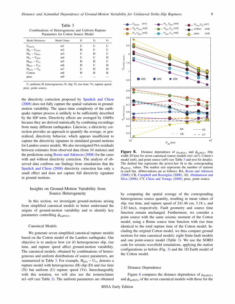
Figure 8 compares the distance dependence of μln�PGV�and ϕln�PGV� of the seven canonical models with those for the

Table 3Combinations of Heterogeneous and Uniform Rupture

Parameters for Cotton Source Model

Model Reference Model Name D Tr Vr

UDTrVr m1 U U UHD − UTrVr m2 H U UHTr − UDVr m3 U H UHVr − UDTr m4 U U HHDTr − UVr m5 H H UHDVr − UTr m6 H U HHTrVr − UD m7 U H HCotton m8 H H Hptsrc m9 — — —

U, uniform; H, heterogeneous; D, slip; Tr, rise time; Vr, rupture speed;ptsrc, point source.

0.5

1

1.5

2

2.5

400 300 200

μ ln(

PG

V (

cm/s

) )

UDTrVr

(m1)

HD

UTrVr

(m2)

HTr

UDVr

(m3)

HVr

UDTr

(m4)

HDTr

UVr

(m5)

HDVr

UTr

(m6)

HTrVr

UD

(m7)

Cotton (m8)

ptsrc (m9)

101

102

0.3

0.4

0.5

0.6

0.7

0.8

0.9

RJB

(km)

φ ln(

PG

V (

cm/s

) )

BA

CB

AS

CY

Figure 8. Distance dependence of μln�PGV� and ϕln�PGV� (binwidth 20 km) for seven canonical source models (m1–m7), Cotton’smodel (m8), and point source (m9) (see Table 3 and text for details).The dashed line represents the power-law fit to the correspondingϕln�PGV� values. The marker size represents the number of stationsin each bin. Abbreviations are as follows: BA, Boore and Atkinson(2008); CB, Campbell and Bozorgnia (2008); AS, Abrahamson andSilva (2008); CY, Chiou and Youngs (2008); ptsrc, point source.

Distance and Azimuthal Dependence of Ground-Motion Variability for Unilateral Strike-Slip Ruptures 9

BSSA Early Edition

Cotton model and the point source. We fit the power law,ϕln�PGV� � αRk

JB, and obtain the values for the parametersα and k by least-squares fitting (see Table 4).

Figure 8 indicates that slip heterogeneity largelycontrols the power-law decay of ϕln�PGV�. All three modelswith heterogeneous slip (i.e., HD − UTrVr, HDTr − UVr, andHDVr − UTr) yield k-values in the −0:13 to −0:10 range, con-sistent with the original Cotton model for which k � −0:13.All other canonical models with uniform slip yield signifi-cantly lower k-values in the −0:03 to 0.01 range, that is,k is so small that the resulting ϕln�PGV� is almost constant.

Figure 8 also suggests that the effects of heterogeneity inrise time (Tr) and rupture velocity (Vr) on ϕln�PGV� depend onthe heterogeneity of slip (D). If slip is heterogeneous, thenneither heterogeneous nor uniform rise time cause sizableeffects on ϕln�PGV�, (compare solutions m5 with m2 or m8with m6). However, if slip is uniform, heterogeneous Trseems to be responsible for lower ϕln�PGV� (compare solu-tions m3 with m1). Similarly, if slip is uniform, hetero-geneous Vr seems to be responsible for lower ϕln�PGV�(compare solutions m4 with m1). However, if both Tr andVr are heterogeneous and slip is uniform, higher ϕln�PGV�is found compared to the cases of only Tr (or Vr) beingheterogeneous (compare solutions m7 with m3 or m7 withm4). This suggests that there is a trade-off between Tr andVr, which is also supported by similar ϕln�PGV� values forHTr − UDVr (m3) and HVr − UDTr (m4). ϕln�PGV� computedfrom simplified models m3 and m4 is close to ϕln�PGV� es-timates for the four GMPEs we use (see Fig. 8 for details).

Next, we analyze ϕln�PGV� for the point-source model.Because of a small number of stations (only 86) for the dis-tance bin RJB � 11 km, we do not consider it statisticallyrobust and excluded it from power-law fitting. Ground-motion variability of a point source is constant with distanceas a consequence of fixed ratio of P- and S-wave amplitudes(because both decay with 1/r). Our results, however, indicatea slow increase of ϕln�PGV� with RJB, as a result of the pres-ence of reflected and refracted body waves, as well as surface

waves, generated by the layered-velocity structure. For largerRJB, ϕln�PGV� is closer to the GMPEs estimates.

From the seven additional finite-fault models, those withheterogeneous slip exhibit a power-law decay with distance,similar to that of the original Cotton model. Uniform-slipmodels yield a substantially smaller slope k. We also findthat slip heterogeneity plays a role in the case of hetero-geneous rise time and rupture speed. Our results indicate thatslip heterogeneity is the controlling parameter for the power-law decay of ground-motion variability for low frequencies(0–0.5 Hz). However, further analysis is required to preciselyquantify effects of slip heterogeneity on the power-law decayof ground-motion variability.

Azimuthal Dependence

Next, we analyze the azimuthal dependence of ϕln�PGV�for the eight simplified rupture models and the originalCotton model (Fig. 9). The distributions of μln�PGV� have asimilar shape to the Cauchy–Lorentz function for the finite-fault models, whereas the point source shows the expectedπ=2 periodic S-wave radiation pattern. We fit the Cauchy–Lorentz function to the azimuthal distributions of μln�PGV�and estimate its parameters (equation 1; see Table 5 and

Table 4Parameters α and k of the Power Law (αRk

JB) Obtained fromLeast-Squares Fitting to the Distance Dependence of

ϕln�PGV� for Nine Sources

Model Reference* Model Name α k

UDTrVr m1 0.56 0.01HD − UTrVr m2 1.16 −0.10HTr − UDVr m3 0.48 0.01HVr − UDTr m4 0.52 −0.01HDTr − UVr m5 1.18 −0.11HDVr − UTr m6 1.02 −0.13HTrVr − UD m7 0.78 −0.03Cotton m8 1.03 −0.13ptsrc m9 0.27 0.13

*U, uniform; H, heterogeneous; D, slip; Tr, rise time; Vr, rupturespeed; ptsrc, point source.

−0.5

0

0.5

1

1.5

2

2.5

3

150 100 50

μ ln(

PG

V (

cm/s

) )

UDTrVr

(m1)

HD

UTrVr

(m2)

HTr

UDVr

(m3)

HVr

UDTr

(m4)

HDTr

UVr

(m5)

HDVr

UTr

(m6)

HTrVr

UD

(m7)

Cotton (m8)

ptsrc (m9)

−180 −135 −90 −45 0 45 90 135 180

0.1

0.2

0.3

0.4

0.5

0.6

0.7

0.8

Azimuth from epicenter (°)

φ ln(

PG

V (

cm/s

) )

Figure 9. Azimuthal dependence of μln�PGV� and ϕln�PGV� (binwidth 15°) for seven canonical source models (m1–m7), Cotton’smodel (m8), and point source (m9) (see Table 3 and text for details).The marker size represents the number of stations in each bin; 0°azimuth represents the average strike direction.

10 J. C. Vyas, P. M. Mai, and M. Galis

BSSA Early Edition

Ⓔ Fig. S6). Table 5 lists the corresponding residual sum ofsquares (RSS) with respect to the fit to the Cotton model. Thefour parameters for the model with heterogeneous slip andrupture speed (HDVr − UTr) are close to the Cotton modelwith lowest RSS. On the other hand, the model with uniformslip and rupture speed (HTr − UDVr) has highest RSS, withlarge deviation from Cotton (Fig. 9 and Ⓔ Fig. S6), indicat-ing that slip and rupture speed control μln�PGV�. The modelwith uniform slip HTrVr − UD shows a broad distribution ofμln�PGV�, hence the highest γ-value. We also observe that risetime has the smallest effect on the shape of Cauchy–Lorentzfunction (compare solutions m6 with m8 or m2 with m5).Thus, the combination of slip and rupture speed controlsthe shape of Cauchy–Lorentz function, with slip being thedominating parameter.

Figure 9 also reveals that ϕln�PGV� of m1–m7 show asimilar pattern as the Cotton model, whereas ϕln�PGV� fromthe point source is periodic due to S-wave radiation pattern.Table 6 lists the RSS values of ϕln�PGV� with respect to theCotton model, showing that ϕln�PGV� from rupture modelm6 with heterogeneous slip and rupture speed is closestto Cotton with lowest RSS (Fig. 9 and Table 6). Modelsm1 and m3 yield a high RSS value, indicating again thatheterogeneity of rise time appears least important. The re-maining four models (m2, m4, m5, and m7) also show largevalues of RSS, but heterogeneous slip leads to significantlylower RSS values for m5 compared to m3, for m6 comparedto m4, and for m2 compared to m1. Heterogeneous rupturespeed leads to significantly lower RSS value for m6 com-pared to m2, for m7 compared to m3, and for m4 comparedto m1. Based on these observations, we conclude that com-bination of slip and rupture speed controls the azimuthal pat-tern of ϕln�PGV�, but at this point it is difficult to assess whichof the two is the dominating parameter.

Mw 7.8 ShakeOut Scenario

Here, we test our hypothesis that ground-motionvariability due to unilateral ruptures with directivity effect

decays as a power law of RJB and that the decay is primarilycontrolled by slip heterogeneity. We also test the hypothesisthat ground-motion variability is high along the rupture-propagation direction, and low along the perpendiculardirection for unilateral ruptures. To this end, we perform sim-ulations for the ShakeOut scenario—a hypothetical Mw 7.8strike-slip earthquake in southern California, with complexfault geometry and heterogeneous rupture process, embeddedin a 3D velocity structure.

Kinematic Source

The ShakeOut project developed several earthquake sce-narios designed to examine physical, social, and economicconsequences of a major earthquake in southern California(Jones et al., 2008). Hypothetically, Mw 7.8 earthquakes areconstructed by compiling information from trenching, pre-historic earthquakes, instrumental recordings, and theoriesof earthquake source physics (Jones et al., 2008). The extentof the fault rupture is determined from geological character-istics. The fault length is 305 km, and rupture depth isslightly variable (average fault width is 14.4 km). We con-sider the case with the hypocenter located near the southernend of the San Andreas fault and for which the rupture prop-agates towards the north. The kinematic rupture process fol-lows the description of Graves et al. (2008), with an averageslip of 4.6 m. The slip distribution is a combination of a char-acterization by Jones et al. (2008) for long length scales(>30 km) and the approach of Mai and Beroza (2002)for short length scales. The source time function is a Brunepulse, with rise time proportional to the square root of slip.Independent source time functions in strike and dip direc-tions allow for temporal rake rotations. Figure 10 showsthe distribution of slip on the fault with local variations ofstrike and dip angles.

Computational Model and Parameters

To replicate the ShakeOut simulation, we use the 3Dvelocity model CVM4 (Kohler et al., 2003) of the SouthernCalifornia Earthquake Center with truncated S-wavespeed(VS min � 620 m=s; the P-wavespeed is then modified such

Table 6RSS of ϕln�PGV� with Respect to Cotton for the Seven Sources

Source Name* Model Name RSS†

UDTrVr m1 1.06HD − UTrVr m2 0.38HTr − UDVr m3 0.77HVr − UDTr m4 0.38HDTr − UVr m5 0.16HDVr − UTr m6 0.03HTrVr − UD m7 0.48

*U, uniform; H, heterogeneous; D, slip; Tr, rise time; Vr, rupture speed;ptsrc, point source.

†RSS, residual sum of squares.

Table 5Parameters I, γ, x0, and C obtained from Nonlinear

Optimization of Fitting the Cauchy–Lorentz Distribution tothe Azimuthal Distribution of μln�PGV� for the Eight Sources

ModelReference*

ModelName

I γ x0 C RSS†

UDTrVr m1 1.93 30.43 5.94 0.8 54.17HD − UTrVr m2 2.62 50.37 7.79 0.18 28.13HTr − UDVr m3 1.66 35.08 8.12 0.94 86.04HVr − UDTr m4 1.71 78.24 12.41 −0.32 62.10HDTr − UVr m5 2.54 47.86 7.1 0.29 32.37HDVr − UTr m6 1.9 58.82 5.69 −0.02 11.23HTrVr − UD m7 3.37 149.52 19.45 −1.48 23.26Cotton m8 2.07 66.59 6.21 0.0 0.00

*U, uniform; H, heterogeneous; D, slip; Tr, rise time; Vr, rupture speed;ptsrc, point source.

†RSS, residual sum of squares.

Distance and Azimuthal Dependence of Ground-Motion Variability for Unilateral Strike-Slip Ruptures 11

BSSA Early Edition

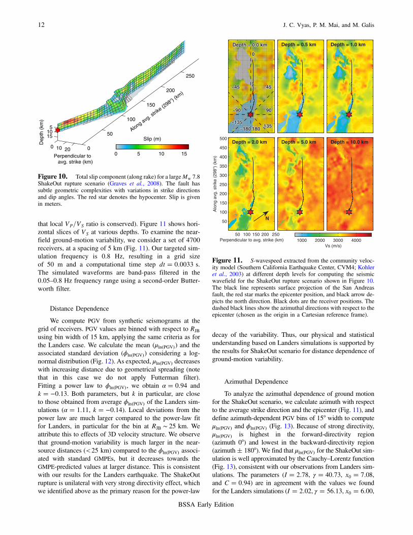
that local VP=VS ratio is conserved). Figure 11 shows hori-zontal slices of VS at various depths. To examine the near-field ground-motion variability, we consider a set of 4700receivers, at a spacing of 5 km (Fig. 11). Our targeted sim-ulation frequency is 0.8 Hz, resulting in a grid sizeof 50 m and a computational time step dt � 0:0033 s.The simulated waveforms are band-pass filtered in the0.05–0.8 Hz frequency range using a second-order Butter-worth filter.

Distance Dependence

We compute PGV from synthetic seismograms at thegrid of receivers. PGV values are binned with respect to RJB

using bin width of 15 km, applying the same criteria as forthe Landers case. We calculate the mean (μln�PGV�) and theassociated standard deviation (ϕln�PGV�) considering a log-normal distribution (Fig. 12). As expected, μln�PGV� decreaseswith increasing distance due to geometrical spreading (notethat in this case we do not apply Futterman filter).Fitting a power law to ϕln�PGV�, we obtain α � 0:94 andk � −0:13. Both parameters, but k in particular, are closeto those obtained from average ϕln�PGV� of the Landers sim-ulations (α � 1:11, k � −0:14). Local deviations from thepower law are much larger compared to the power-law fitfor Landers, in particular for the bin at RJB ∼ 25 km. Weattribute this to effects of 3D velocity structure. We observethat ground-motion variability is much larger in the near-source distances (<25 km) compared to the ϕln�PGV� associ-ated with standard GMPEs, but it decreases towards theGMPE-predicted values at larger distance. This is consistentwith our results for the Landers earthquake. The ShakeOutrupture is unilateral with very strong directivity effect, whichwe identified above as the primary reason for the power-law

decay of the variability. Thus, our physical and statisticalunderstanding based on Landers simulations is supported bythe results for ShakeOut scenario for distance dependence ofground-motion variability.

Azimuthal Dependence

To analyze the azimuthal dependence of ground motionfor the ShakeOut scenario, we calculate azimuth with respectto the average strike direction and the epicenter (Fig. 11), anddefine azimuth-dependent PGV bins of 15° width to computeμln�PGV� and ϕln�PGV� (Fig. 13). Because of strong directivity,μln�PGV� is highest in the forward-directivity region(azimuth 0°) and lowest in the backward-directivity region(azimuth� 180°). We find that μln�PGV� for the ShakeOut sim-ulation is well approximated by the Cauchy–Lorentz function(Fig. 13), consistent with our observations from Landers sim-ulations. The parameters (I � 2:78, γ � 40:73, x0 � 7:08,and C � 0:94) are in agreement with the values we foundfor the Landers simulations (I � 2:02, γ � 56:13, x0 � 6:00,

0 10 20 0

50

100

150

200

250

51015

Along avg. s

trike (2

98°) (km

)

Perpendicular to avg. strike (km)

Dep

th (

km)

Slip (m)

0 5 10 15

Figure 10. Total slip component (along rake) for a largeMw 7.8ShakeOut rupture scenario (Graves et al., 2008). The fault hassubtle geometric complexities with variations in strike directionsand dip angles. The red star denotes the hypocenter. Slip is givenin meters.

Depth = 0.0 kmDepth = 0.0 kmDepth = 0.0 kmDepth = 0.0 kmDepth = 0.0 km

00000

4545454545

9090909090

135135135135135180180180180180

−45−45−45−45−45

−90−90−90−90−90

−135−135−135−135−135−180−180−180−180−180

Depth = 0.5 km Depth = 1.0 km

Depth = 2.0 km

Perpendicular to avg. strike (km)

Alo

ng a

vg. s

trik

e (2

98°)

(km

)N

50 100 150 200 250

50

100

150

200

250

300

350

400

450

500Depth = 5.0 km Depth = 10.0 km

Vs (m/s)1000 2000 3000 4000

Figure 11. S-wavespeed extracted from the community veloc-ity model (Southern California Earthquake Center, CVM4; Kohleret al., 2003) at different depth levels for computing the seismicwavefield for the ShakeOut rupture scenario shown in Figure 10.The black line represents surface projection of the San Andreasfault, the red star marks the epicenter position, and black arrow de-picts the north direction. Black dots are the receiver positions. Thedashed black lines show the azimuthal directions with respect to theepicenter (chosen as the origin in a Cartesian reference frame).

12 J. C. Vyas, P. M. Mai, and M. Galis

BSSA Early Edition

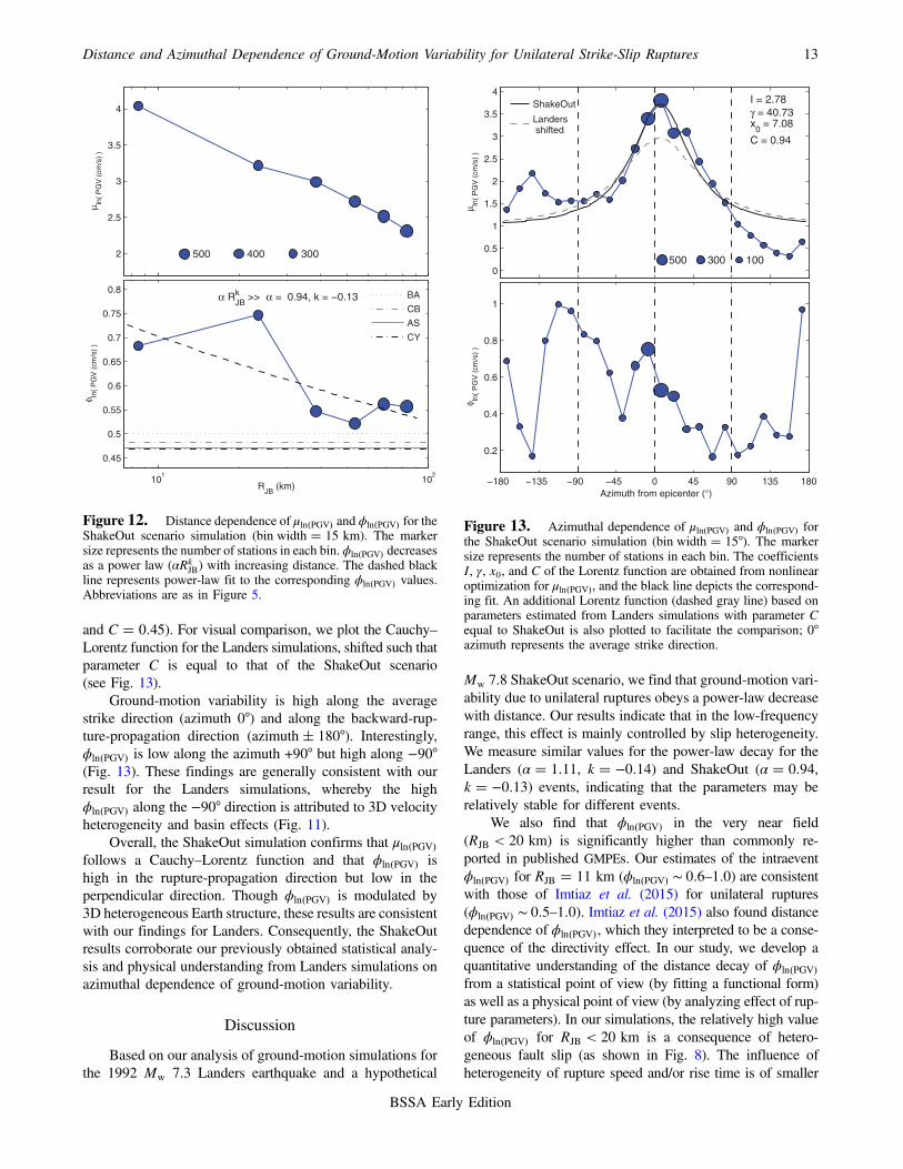
and C � 0:45). For visual comparison, we plot the Cauchy–Lorentz function for the Landers simulations, shifted such thatparameter C is equal to that of the ShakeOut scenario(see Fig. 13).

Ground-motion variability is high along the averagestrike direction (azimuth 0°) and along the backward-rup-ture-propagation direction (azimuth� 180°). Interestingly,ϕln�PGV� is low along the azimuth +90° but high along −90°(Fig. 13). These findings are generally consistent with ourresult for the Landers simulations, whereby the highϕln�PGV� along the −90° direction is attributed to 3D velocityheterogeneity and basin effects (Fig. 11).

Overall, the ShakeOut simulation confirms that μln�PGV�follows a Cauchy–Lorentz function and that ϕln�PGV� ishigh in the rupture-propagation direction but low in theperpendicular direction. Though ϕln�PGV� is modulated by3D heterogeneous Earth structure, these results are consistentwith our findings for Landers. Consequently, the ShakeOutresults corroborate our previously obtained statistical analy-sis and physical understanding from Landers simulations onazimuthal dependence of ground-motion variability.

Discussion

Based on our analysis of ground-motion simulations forthe 1992 Mw 7.3 Landers earthquake and a hypothetical

Mw 7.8 ShakeOut scenario, we find that ground-motion vari-ability due to unilateral ruptures obeys a power-law decreasewith distance. Our results indicate that in the low-frequencyrange, this effect is mainly controlled by slip heterogeneity.We measure similar values for the power-law decay for theLanders (α � 1:11, k � −0:14) and ShakeOut (α � 0:94,k � −0:13) events, indicating that the parameters may berelatively stable for different events.

We also find that ϕln�PGV� in the very near field(RJB < 20 km) is significantly higher than commonly re-ported in published GMPEs. Our estimates of the intraeventϕln�PGV� for RJB � 11 km (ϕln�PGV� ∼ 0:6–1:0) are consistentwith those of Imtiaz et al. (2015) for unilateral ruptures(ϕln�PGV� ∼ 0:5–1:0). Imtiaz et al. (2015) also found distancedependence of ϕln�PGV�, which they interpreted to be a conse-quence of the directivity effect. In our study, we develop aquantitative understanding of the distance decay of ϕln�PGV�from a statistical point of view (by fitting a functional form)as well as a physical point of view (by analyzing effect of rup-ture parameters). In our simulations, the relatively high valueof ϕln�PGV� for RJB < 20 km is a consequence of hetero-geneous fault slip (as shown in Fig. 8). The influence ofheterogeneity of rupture speed and/or rise time is of smaller

2

2.5

3

3.5

4

500 400 300

μ ln(

PG

V (

cm/s

) )

101

102

0.45

0.5

0.55

0.6

0.65

0.7

0.75

0.8

RJB

(km)

φ ln(

PG

V (

cm/s

) )

α RJBk >> α = 0.94, k = −0.13 BA

CB

AS

CY

Figure 12. Distance dependence of μln�PGV� and ϕln�PGV� for theShakeOut scenario simulation (bin width � 15 km). The markersize represents the number of stations in each bin. ϕln�PGV� decreasesas a power law (αRk

JB) with increasing distance. The dashed blackline represents power-law fit to the corresponding ϕln�PGV� values.Abbreviations are as in Figure 5.

0

0.5

1

1.5

2

2.5

3

3.5

4 I = 2.78 γ = 40.73 x

0 = 7.08

C = 0.94

μ ln(

PG

V (

cm/s

) )

500 300 100

ShakeOut

Landers shifted

−180 −135 −90 −45 0 45 90 135 180

0.2

0.4

0.6

0.8

1

Azimuth from epicenter (°)

φ ln(

PG

V (

cm/s

) )

Figure 13. Azimuthal dependence of μln�PGV� and ϕln�PGV� forthe ShakeOut scenario simulation (bin width � 15°). The markersize represents the number of stations in each bin. The coefficientsI, γ, x0, and C of the Lorentz function are obtained from nonlinearoptimization for μln�PGV�, and the black line depicts the correspond-ing fit. An additional Lorentz function (dashed gray line) based onparameters estimated from Landers simulations with parameter Cequal to ShakeOut is also plotted to facilitate the comparison; 0°azimuth represents the average strike direction.

Distance and Azimuthal Dependence of Ground-Motion Variability for Unilateral Strike-Slip Ruptures 13

BSSA Early Edition

importance. We further expect that other factors, such as faultroughness, seismic scattering, or plastic deformation, may alsoaffect the behavior of ϕln�PGV� in near field. Fault roughnesscauses local stress perturbations, leading to localized acceler-ations and decelerations of the rupture front (Madariaga,1977), and promotes self-healing pulses (Shi and Day, 2013),leading to increased high-frequency radiation that affects near-field ground motion. Small-scale heterogeneities in Earthstructure produce significant high-frequency seismic-wavescattering (Imperatori and Mai, 2013), which results in an ap-parent isotropic, instead of four-lobed, S-wave radiation pat-tern (Takemura et al., 2009). Inclusion of plastic deformationin rupture dynamics leads to slip-rate saturation and a shift ofthe corner-frequency towards lower frequencies comparedwith the elastic case (Andrews, 2005; Shi and Day, 2013). Weconjecture that fault roughness and seismic scattering increasenear-field ground-motion variability, whereas plasticity maylead to decreased ϕln�PGV�.

In the far field (RJB ∼ 100 km), the ϕln�PGV� values esti-mated from simulations converge to the values of ϕln�PGV�given in standard GMPEs. The higher near-field ground-motionvariability inferred from simulations may have significant im-pact on seismic-hazard estimation because the annual frequencyof exceedance is highly sensitive to the ϕln�PGV�, particularly forlong return periods (Bommer and Abrahamson, 2006). Our re-sults suggest that PGV values estimated using standard GMPEswith constant ϕln�PGV� may be underestimated in the very nearfield in the case of unilateral and directive ruptures.

Our analyses for the 1992 Landers earthquake andShakeOut scenario simulations show that intraevent ground-motion variability for unilateral directive ruptures is high inboth the forward- and backward-directivity direction but lowin the direction perpendicular to rupture propagation. In ad-dition, we observe that the azimuthal dependency of ϕln�PGV�is controlled by both rupture speed and slip, but slip hetero-geneity seems to be the dominating parameter. Rippergeret al. (2008) found that the interevent ground-motion vari-ability is strongest in the backward-directivity region, butthey have not analyzed the intraevent ground-motion vari-ability. However, it appears that both the intraevent andinterevent ground-motion variability follow similar patterns.We also observe that μln�PGV� can be modeled using aCauchy–Lorentz distribution, which captures the effects ofstrong seismic radiation in the forward-rupture-propagationdirection due to directivity.

We find that ϕln�PGV� is a function of both distance andazimuth for the Landers earthquake and the ShakeOutscenario for relatively low frequencies (up to 0.5 and 0.8 Hz,respectively). However, high frequencies (up to 25 Hz) areimportant for engineering purposes and seismic-hazard esti-mation. For high frequencies, the effects of seismic-wavescattering have to be included (e.g., Imperatori and Mai,2013). These affect ground motions and their variabilityalready at short distances, at which generally source effectsare thought to dominate. Further investigations of ground-motion variability, considering scattering and more complex

3D velocity structures as well as multiple-realistic earth-quake-rupture realizations, are needed to better understandthe effects of scattering on ground-motion variability for lowand high frequencies.

Conclusions

Ground-motion variability ϕln�PGV� estimated fromnumerical simulations of the 1992 Mw 7.3 Landers earth-quake and the Mw 7.8 ShakeOut scenario is higher in thenear field (RJB < 20 km) compared to standard GMPEs. Thissignificantly affects probabilistic seismic-hazard assessment,especially for long periods and in the presence of faults thatare capable of generating large unilateral earthquake withstrong directivity. ϕln�PGV� decreases with increasing RJB dis-tance from the fault as a power law (αRk

JB) and approachesvalues of ϕln�PGV� estimated by GMPEs at large distances(RJB ∼ 100 km). High values of ϕln�PGV� in near-source dis-tances are caused by a strong directivity effect. Farther awayfrom the fault, the effect of directivity on ground motion di-minishes. Consequently, also ϕln�PGV� decreases. Our analy-ses suggest that the power-law decay of ϕln�PGV� is mainlycontrolled by slip heterogeneity. We also show that intrae-vent ground-motion variability for unilateral ruptures is largein both the forward- and backward-rupture-propagation di-rection but low in the direction perpendicular to rupturepropagation. We find that ϕln�PGV� as a function of azimuthis sensitive to slip heterogeneity as well as rupture speed var-iations, but the effects of the on-fault slip heterogeneity seemto dominate over the influence of rupture speed. We demon-strate that μln�PGV� as a function of azimuth is well describedby a Cauchy–Lorentz distribution, which provides a novelapproach to better predict the spatial dependencies ofground-motion variability for engineering purposes.

Data and Resources

The five kinematic rupture models of the 1992 Landersearthquake are obtained from the Earthquake Source ModelDatabase (SRCMOD; Mai and Thingbaijam, 2014) accessibleonline at http://equake‑rc.info/SRCMOD/ (last accessedMarch2016). The recorded seismograms of the earthquake were ob-tained from the Consortium of Organizations for Strong Mo-tion Observation Systems (COSMOS) database accessible athttp://cosmos-eq.org/VDC/index.html (last accessed March2016). The Southern California Earthquake Center communityvelocity model CVM4 (Kohler et al., 2003) employed for theShakeOut simulations is accessible at http://scedc.caltech.edu/research-tools/3d-velocity.html (last accessed March 2016).MATLAB scripts were accessed from www.mathworks.com/products/matlab (last accessed May 2016).

Acknowledgments

We thank Rob Graves for providing us with the source model of theShakeOut scenario and Paul Spudich for sharing with us his MATLAB

14 J. C. Vyas, P. M. Mai, and M. Galis

BSSA Early Edition

scripts to compute the directivity corrections. We thank Fabrice Cotton forhis critical review that helped us to improve the manuscript. We also thankKiran Kumar Thingbaijam for insightful discussions. The research pre-sented in this article is supported by King Abdullah University of Scienceand Technology (KAUST) in Thuwal, Saudi Arabia. Earthquake ruptureand ground-motion simulations have been carried out using the KAUSTSupercomputing Laboratory (KSL), and we acknowledge the support ofthe KSL staff.

References

Abrahamson, N., and W. Silva (2008). Summary of the Abrahamson & SilvaNGA ground-motion relations, Earthq. Spectra 24, no. 1, 67–97.

Akkar, S., and J. J. Bommer (2007a). Empirical prediction equations forpeak ground velocity derived from strong-motion records from Europeand the Middle East, Bull. Seismol. Soc. Am. 97, no. 2, 511–530.

Akkar, S., and J. J. Bommer (2007b). Prediction of elastic displacementresponse spectra in Europe and the Middle East, Earthq. Eng. Struct.Dynam. 36, no. 10, 1275–1301.

Anderson, J. G., and J. N. Brune (1999). Probabilistic seismic hazardanalysis without the ergodic assumption, Seismol. Res. Lett. 70,no. 1, 19–28.

Andrews, D. J. (2005). Rupture dynamics with energy loss outside the slipzone, J. Geophys. Res. 110, no. B1, doi: 10.1029/2004JB003191.

Atkinson, G. (2013). Empirical evaluation of aleatory and epistemicuncertainty in eastern ground motions, Seismol. Res. Lett. 84, no. 1,130–138.

Bindi, D., M. Massa, L. Luzi, G. Ameri, F. Pacor, R. Puglia, and P. Augliera(2014). Pan-European ground-motion prediction equations for theaverage horizontal component of PGA, PGV, and 5%-damped PSAat spectral periods up to 3.0 s using the RESORCE dataset, Bull.Earthq. Eng. 12, no. 1, 391–430.

Boatwright, J. (2007). The persistence of directivity in small earthquakes,Bull. Seismol. Soc. Am. 97, no. 6, 1850–1861.

Bommer, J. J., and N. A. Abrahamson (2006). Why do modern probabilisticseismic-hazard analyses often lead to increased hazard estimates? Bull.Seismol. Soc. Am. 96, no. 6, 1967–1977.

Boore, D. M., and G. M. Atkinson (2008). Ground-motion predictionequations for the average horizontal component of PGA, PGV, and5%-damped PSA at spectral periods between 0.01 s and 10.0 s, Earthq.Spectra 24, no. 1, 99–138.

Boore, D. M., W. B. Joyner, and T. E. Fumal (1997). Equations for estimat-ing horizontal response spectra and peak acceleration from westernNorth American earthquakes: A summary of recent work, Seismol.Res. Lett. 68, no. 1, 128–153.

Boore, D. M., J. P. Stewart, E. Seyhan, and G. M. Atkinson (2014). NGA-West2 equations for predicting PGA, PGV, and 5% damped PSA forshallow crustal earthquakes, Earthq. Spectra 30, no. 3, 1057–1085.

Boore, D. M., J. Watson-Lamprey, and N. A. Abrahamson (2006). Orienta-tion-independent measures of ground motion, Bull. Seismol. Soc. Am.96, no. 4A, 1502–1511.

Campbell, K. W., and Y. Bozorgnia (2008). NGA ground motion model forthe geometric mean horizontal component of PGA, PGV, PGD and 5%damped linear elastic response spectra for periods ranging from 0.01 to10 s, Earthq. Spectra 24, no. 1, 139–171.

Chiou, B. S. J., and R. R. Youngs (2006). Chiou and Youngs PEER-NGAempirical ground motion model for the average horizontal componentof peak acceleration and pseudo-spectral acceleration for spectralperiods of 0.01 to 10 seconds, PEER Report Draft, Pacfic EarthquakeEngineering Research Centre, Berkeley, California.

Chiou, B. S. J., and R. R. Youngs (2008). An NGA model for the averagehorizontal component of peak ground motion and response spectra,Earthq. Spectra 24, no. 1, 173–215.

Cohee, B. P., and G. C. Beroza (1994). Slip distribution of the 1992 Landersearthquake and its implications for earthquake source mechanics, Bull.Seismol. Soc. Am. 84, no. 3, 692–712.

Cotton, F., and M. Campillo (1995). Frequency domain inversion of strongmotions: Application to the 1992 Landers earthquake, J. Geophys. Res.100, no. B3, 3961–3975.

Dumbser, M., and M. Käser (2006). An arbitrary high-order discontinuousGalerkin method for elastic waves on unstructured meshes: II.The three-dimensional isotropic case, Geophys. J. Int. 167, no. 1,319–336.

Ely, G. P., S. M. Day, and J. B. Minster (2008). A support-operator methodfor viscoelastic wave modelling in 3-D heterogeneous media,Geophys. J. Int. 172, no. 1, 331–344.

Graves, R. W., B. T. Aagaard, K. W. Hudnut, L. M. Star, J. P. Stewart, and T.H. Jordan (2008). Broadband simulations for Mw 7.8 southern SanAndreas earthquakes: Ground motion sensitivity to rupture speed,Geophys. Res. Lett. 35, no. 22, doi: 10.1029/2008GL035750.

Henry, C., and S. Das (2001). Aftershock zones of large shallowearthquakes: Fault dimensions, aftershock area expansion and scalingrelations, Geophys. J. Int. 147, no. 2, 272–293.

Hernandez, B., F. Cotton, and M. Campillo (1999). Contribution of radarinterferometry to a two-step inversion of the kinematic process of the1992 Landers earthquake, J. Geophys. Res. 104, no. B6, 13,083–13,099.

Imperatori, W., and P. M. Mai (2012). Sensitivity of broad-band ground-motion simulations to earthquake source and Earth structure variations:An application to the Messina Straits (Italy), Geophys. J. Int. 188,no. 3, 1103–1116.

Imperatori, W., and P. M. Mai (2013). Broad-band near-field ground motionsimulations in 3-dimensional scattering media, Geophys. J. Int. 192,no. 2, 725–744.

Imtiaz, A., M. Causse, E. Chaljub, and F. Cotton (2015). Is ground-motionvariability distance dependent? Insight from finite-source rupture sim-ulations, Bull. Seismol. Soc. Am. 105, no. 2A, 950–962.

Jones, L. M., R. Bernknopf, D. Cox, J. Goltz, K. Hudnut, D. Mileti, S. Perry,D. Ponti, K. Porter, M. Reichle, et al. (2008). The ShakeOut Scenario,U.S. Geol. Surv. Open-File Rept. 2008-1150 and California Geol.Surv. Preliminary Report 25, http://pubs.usgs.gov/of/2008/1150/ (lastaccessed May 2016).

Kohler, M. D., H. Magistrale, and R. W. Clayton (2003). Mantle hetero-geneities and the SCEC reference three-dimensional seismic velocitymodel version 3, Bull. Seismol. Soc. Am. 93, no. 2, 757–774.

Komatitsch, D., and J. Tromp (1999). Introduction to the spectral elementmethod for three-dimensional seismic wave propagation, Geophys. J.Int. 139, no. 3, 806–822.

Madariaga, R. (1977). High-frequency radiation from crack (stress drop)models of earthquake faulting, Geophys. J. Int. 51, no. 3, 625–651.

Mai, P. M (2009). Ground motion: Complexity and scaling in the near fieldof earthquake ruptures, in Encyclopedia of Complexity and SystemsScience, W. H. K. Lee and R. Meyers (Editors), Springer, New York,4435–4474.

Mai, P. M., and G. C. Beroza (2002). A spatial random field model tocharacterize complexity in earthquake slip, J. Geophys. Res. 107,no. B11, 2308.

Mai, P. M., and K. K. S. Thingbaijam (2014). SRCMOD: An online databaseof finite-fault rupture models, Seismol. Res. Lett. 85, no. 6, 1348–1357.

Mai, P. M., W. Imperatori, and K. B. Olsen (2010). Hybrid broadbandground-motion simulations: Combining long-period deterministicsynthetics with high-frequency multiple S-to-S backscattering, Bull.Seismol. Soc. Am. 100, no. 5A, 2124–2142.

Mai, P. M., P. Spudich, and J. Boatwright (2005). Hypocenter locationsin finite-source rupture models, Bull. Seismol. Soc. Am. 95, no. 3,965–980.

McGuire, J. J., L. Zhao, and T. H. Jordan (2002). Predominance of unilateralrupture for a global catalog of large earthquakes, Bull. Seismol. Soc.Am. 92, no. 8, 3309–3317.

Mena, B., and P. M. Mai (2011). Selection and quantification of near-faultvelocity pulses owing to source directivity, Georisk 5, no. 1, 25–43.

Ramirez-Guzman, L., R. W. Graves, K. B. Olsen, O. S. Boyd, C. Cramer, S.Hartzell, S. Ni, P. Somerville, R. A. Williams, and J. Zhong (2015).

Distance and Azimuthal Dependence of Ground-Motion Variability for Unilateral Strike-Slip Ruptures 15

BSSA Early Edition

Ground-motion simulations of 1811–1812 New Madrid earthquakes,central United States, Bull. Seismol. Soc. Am. 105, no. 4, 1961–1988.

Ripperger, J., P. M. Mai, and J. P. Ampuero (2008). Variability of near-fieldground motion from dynamic earthquake rupture simulations, Bull.Seismol. Soc. Am. 98, no. 3, 1207–1228.

Rodriguez-Marek, A., G. A. Montalva, F. Cotton, and F. Bonilla (2011).Analysis of single-station standard deviation using the KiK-net data,Bull. Seismol. Soc. Am. 101, no. 3, 1242–1258.

Seekins, L. C., and J. Boatwright (2010). Rupture directivity of moderateearthquakes in northern California, Bull. Seismol. Soc. Am. 100,no. 3, 1107–1119.

Shi, Z., and S. M. Day (2013). Rupture dynamics and ground motion from3-D rough-fault simulations, J. Geophys. Res. 118, no. 3, 1122–1141.

Somerville, P. G., N. F. Smith, R. W. Graves, and N. A. Abrahamson (1997).Modification of empirical strong ground motion attenuation relationsto include the amplitude and duration effects of rupture directivity,Seismol. Res. Lett. 68, no. 1, 199–222.

Spudich, P., and B. S. Chiou (2008). Directivity in NGA earthquake groundmotions: Analysis using isochrone theory, Earthq. Spectra 24, no. 1,279–298.

Spudich, P., and L. N. Frazer (1984). Use of ray theory to calculate high-frequency radiation from earthquake sources having spatially variablerupture velocity and stress drop, Bull. Seismol. Soc. Am. 74, no. 6,2061–2082.

Strasser, F. O., N. A. Abrahamson, and J. J. Bommer (2009). Sigma: Issues,insights, and challenges, Seismol. Res. Lett. 80, no. 1, 40–56.

Takemura, S., T. Furumura, and T. Saito (2009). Distortion of the apparentS-wave radiation pattern in the high-frequency wavefield: Tottori-kenSeibu, Japan, earthquake of 2000, Geophys. J. Int. 178, no. 2, 950–961.

Varela, C. L., A. L. Rosa, and T. J. Ulrych (1993). Modeling of attenuationand dispersion, Geophysics 58, no. 8, 1167–1173.

Wald, D. J., and T. H. Heaton (1994). Spatial and temporal distribution ofslip for the 1992 Landers, California, earthquake, Bull. Seismol. Soc.Am. 84, no. 3, 668–691.

Youngs, R. R., N. Abrahamson, F. I. Makdisi, and K. Sadigh (1995).Magnitude-dependent variance of peak ground acceleration, Bull.Seismol. Soc. Am. 85, no. 4, 1161–1176.

Zeng, Y., and J. G. Anderson (2000). Evaluation of numerical proceduresfor simulating near-fault long-period ground motions using Zengmethod, Pacific Earthquake Engineering Research Center, availableat http://peer.berkeley.edu/ (last accessed May 2016).

King Abdullah University of Science and TechnologyDivision of Physical Sciences and EngineeringThuwal 23955-6900Kingdom of Saudi ArabiaJagdish.Vyas@kaust.edu.sa

Manuscript received 29 October 2015;Published Online 21 June 2016

16 J. C. Vyas, P. M. Mai, and M. Galis

BSSA Early Edition