- 1 -

Discriminatory vs Uniform Price Auction: Auction Revenue Comparison in the Case of the Korean Treasury Auction Market

by

Gyung-Rok Kim Mirae Asset Co., Korea

and Seonghwan Oh

Dept. of Economics Seoul National University

and Keunkwan Ryu*

Dept. of Economics Seoul National University

July 14, 2003 (revised February 26, 2004)

Abstract: We compare auction revenues from discriminatory auctions and uniform price auctions in the case of the Korean treasury bonds auction market. For this purpose, we employ detailed bidder level data for each of 16 discriminatory auctions recently carried out in Korea. We first theoretically recover unobserved individual bidding functions under counter-factual uniform price auctions from the observed bidding functions under the actual discriminatory auctions, and then empirically estimate revenue differences. To test significance of the auction revenue differences, we use Bootstrap re-sampling methods where uncertainty in the cut-off yield spreads and uncertainty in the bidders are addressed individually as well as simultaneously. Our results indicate that uniform price auction increases the auction revenue relative to the discriminatory auction in most of the 16 cases, justifying the Korean government’s decision to switch to the uniform price auction mechanism.

Keywords: Treasury bonds auction, discriminatory auction, uniform price auction, hazard rate, Bootstrap re-sampling, yield spread, bidding function, bid shading

JEL Classification: D44, C51, C81

* Correspondence to Keunkwan Ryu, Department of Economics, Seoul National University, Seoul 151-

742, Korea. The first draft of this paper was prepared while the corresponding author was visiting ISER,

Osaka University, summer 2003. Ryu would like to thank Charles Horioka for his hospitality and helpful

comments.

- 2 -

1. Introduction

We compare auction revenues from discriminatory auctions and uniform price auctions in the

case of the Korean treasury bonds auction market. For this purpose, we use detailed bidder level data

for each of 16 discriminatory auctions recently carried out in Korea. Using a theoretical model, we

first recover unobserved individual bidding functions under counter-factual uniform price auctions

from the observed bidding functions under actual discriminatory auctions, and then estimate the

auction revenue differences. To test significance of the auction revenue differences, we use

Bootstrapping re-sampling methods by which we address uncertainty in the cut-off yield spreads as

well as uncertainty in the bidders. Our results indicate that the uniform price auction increases the

auction revenue relative to the discriminatory auction in most of the 16 cases analyzed, justifying the

Korean government’s decision to switch to the uniform price auction in the year 2000.

Let us briefly overview the Korean treasury auction market. The Korean government has

adopted a competitive bidding system in the treasury bonds auction market, September 1999. There

exist 24 primary dealers and 6 candidate dealers for a total of 30 dealers who are exclusively entitled

to submitting bids in the Korean treasury auction. The Korean treasury has nominated 6 candidate

dealers for the purpose of “internship” before promoting them to primary dealers. Most of the 30

dealers are either banks or security companies. Their market powers are evenly distributed in terms of

bidding and winning amounts. The Korean treasury auction market is competitive.

Under the discriminatory auction, “what you bid is what you pay.” The bigger the uncertainty

about the auction cut-off price, the less willing you become to bid, so called “bid shading.” Bid

shading is more severe as the uncertainty in the cut-off price increases. Lack of the so called “when-

issued market” delays the price discovery process in the Korean treasury auction market on one hand,

whereas it precludes the possibility “short squeeze” on the other.

- 3 -

Depending on whether the uncertainty is large or not, auction revenue criterion favors either

the switch to the uniform price auction or the continuation of the discriminatory auction. We use

historical auction spread distribution as a measure of the uncertainty in the treasury auction market.

We only use those auction spreads that are observed under historical discriminatory auction cases.

Using this measure of auction uncertainty, we identify the magnitude of bid shading and thus revenue

gap between the actual discriminatory auction and the counter-factual uniform price auction for each

of the 16 discriminatory auction cases actually implemented recently in Korea.

The rest of the paper is organized as follows. Section 2 briefly reviews the existing literature

on the treasury bond auction. Section 3 introduces a standard auction model showing the differences in

bidder behavior under the two different auction mechanisms. Section 4 explains the data and the

econometric model. Results are reported in section 5. Section 6 concludes.

2. Literature Review

Auction revenue depends on the underlying auction mechanism. Under a set of conditions,

Vickery (1961) shows that the auction revenue is the same whether one uses a first price auction or a

second price auction. This famous “revenue equivalence theorem,” however, does not hold in divisible

multiple unit auctions as in the case of the treasury bond auction. Revenue comparison becomes even

more difficult as one considers the common value aspect of the treasury bond. Earlier, Friedman

(1960) raises a possibility that the uniform price auction may result in more auction revenues than the

multiple price auction.

Milgrom and Weber (1982), Bikchandani and Huang (1989, 1993), and Chari and Weber

(1992) analyze the treasury auction market. Wilson (1979), Back and Zender (1993), and Wang and

Zender (1996) introduces a divisible goods assumption to make their analyses compartible with the

- 4 -

treasury auction.

Bikchandani and Huang (1989), and Chatterjea and Jarrow (1998) analyze the interaction

between the primary and the seconary markets. According to Bikchandani and Huang (1989), bidders

with maket power would like to bid more aggressively in the primary (auction) market to signal their

strong valuation to the secondary market, and in fact they do so at a lower cost under the uniform price

auction. Chatterjea and Jarrow (1998) argue that bidders with market power bid more aggressively in

the primary market to squeeze out those auction participants with a short position in the “when issued

markets,” so called a “short squeeze” phenomenon.

Viswanathan and Wang (1998) view the primary dealers as market makers in the treasury

auction market.

As theoretical approaches do not provide any conclusive results, there have arisen empirical

approaches to compare auction revenues across the discriminatory and the uniform price auctions.

Most empirical studies compare the observed auction spreads across those two auction mechanisms.

Umlauf (1993a) reports that the Mexican government’s auction revenue slightly increased as Mexico

switched its treasury auction mechanism from the discriominatory one to the uniform one. Regarding

the US, Simon (1994) reports that the auction revenue decreased as the US government switched its

auction mechanism from the discriminatory to the unifrorm in the 70s, whereas Nyborg and

Sundaresan (1996) and Malvey and Archibald (1998) report that the auction revenue increased under

the uniform price auction in the 90s (statistically not significant, though).

Applicability of these empirical approaches is limited in the following two senses. First, they

cannot be used unless a country has experimented both auction mechanisms. Second, they do not use

detailed, micro-level bidding information. An alternative structural approach overcomes these

drawbacks. The structural approaches recover “counter-factual” bidding fuctions under the uniform

price auction from the observed bidding functions from the discriminatory auction. The approach can

- 5 -

be applied even to a country which has only experienced the discrominatory auction mechanism. The

structural approach relies on micro level bidding information to recover the counter-factual bidding

function.

Nautz (1995) develops a theoretical model for the above structual approach. Heller and

Lengwiller (1998) analyze the Swiss treasury auction using the structual approach. Hortacsu (2002a,b)

adds strategic interactions among the bidders to the structural approach.

3. Theoretical Model

Treasury auction is a multiple unit, divisible goods auction. The treasury, as auctioneer, puts

on the table a fixed amount of Treasury bonds. In the Korean treasury auction market, there are a total

of 30 potential bidders who are more or less homogeneous. We assume that each bidder has a common

belief on the distribution of the cut-off price in the auction, and that there are no strategic interactions

either between auctioneers and the bidders or among the bidders. We consider a private value auction

model where different bidders’ private values are not affiliated (Milgrom and Weber 1982).

To be able to recover unobserved bidding behaviors under the counter-factual uniform price

auction from the observed behaviors under the actually implemented discriminatory auction, we need

to characterize theoretically bidders’ bidding behaviors under each auction mechanism and to identify

their relationship.

Section 2.1 introduces the basics. Sections 2.2 and 2.3 characterize the bidding behaviors

under the discriminatory and the uniform price auctions. Section 2.4 recovers the bidding function

under the counter-factual uniform price auction from the bidding function under the actual

discriminatory auction.

- 6 -

3.1. Basics

Bidders determine their bidding strategy to maximize their expected profits. Each bidder is

allowed to submit up to five (price, quantity) pairs. The bidding prices are denominated in terms of

yield to maturity with a tick size of one basis point, that is, one hundredth of one percent point.

Let },,{ 1 kppP = be the support of the market clearing cut-off yield spread, say p . We

arrange jp ’s in an increasing order, kpp <<1 . As a result a more aggressive bid corresponds to a

lower value of jp .

The yield spread is the difference between the market clearing yield (so called the cut-off

yield) and the secondary market yield of the same class of treasury bonds (at morning close on the

same day). A higher yield spread means a higher yield to the bidders relative to the yield anticipated

from the secondary market, and a lower bond price to the treasury.

Let the yield spread distribution (under the discriminatory auction) be represented by

),,( 11 −= kfff , where )Pr( 11 ppf == , ⋅⋅⋅, )Pr( 11 −− == kk ppf . Of course, one has

)(1)Pr( 11 −++−== kk ffpp . For notational consistency, let us denote this value as kf . We

assume that 0)Pr( >= jpp for each of kj ,,1= .* The yield spread distribution can be

equivalently represented as a 1)1( ×−k vector ),,( 11 −= khhh of the so called hazard rates,

where )/( kjjj fffh ++= , 1,,1 −= kj Let us further define 00 =h and 1=kh for later

use.

The hazard rate is the most important concept in life-time, mortality, and duration analyses. It

is the conditional probability of “death” given survival up to now. To understand this concept, imagine

* In the empirical implementation, we only consider those support points jp ’s where bids are ever made in the historical

data, justifying the assumption 0)Pr( >= jpp for each of kj ,,1= .

- 7 -

that you are conducting an “ascending yield” auction. Define death as the end of the auction process.

The auction ends as soon as the total amount of bids exceeds the fixed total supply. Hazard rate at a

given yield spread denotes the chance that the game ends exactly at that yield spread level conditional

on that the auctioneer has just announced that level after passing all the previous levels. At a low

enough yield spread level, say 0p , no bidder would bid. According to the common belief, the chance

that the auction process ends at that low level is zero, 00 =h . On the other hand, suppose you have

already reached a highest possible yield spread level, say kp . At kp , every bidder would bid so far

as the bid is beneficial from her own perspective. According to the common belief, the chance that the

auction process ends immediately at that high level is one, resulting in 1=kh .

Let i index individual bidders in a given discriminatory auction case, ni ,,1= . Bidder

i submits up to a maximum of 5 pairs of price and quantity, ),( ijijp ∆ , imj ,,1= where im is

the number of bids submitted by bidder i . Of course, by regulation, }5,4,3,2,1{∈im . From

imjijijp ,,1},{ =∆ , one can construct bidder i ’s individual bidding function as a step function with im

steps. Let )( ji pb be the amount of bid submitted by bidder i at or below the yield spread jp and

denote it simply as ijb . Do not forget that we are measuring the “price” using the yield spread which

is inversely related with the bond price. We have ∑≤

∆=jij ppj

ijji pb':'

')( , Let )()( jii pbpb = for

1+<≤ jj ppp ( 1,,1 −= kj ), 0)( =pbi for 1pp < and )()( kii pbpb = for kpp ≥ . It

represents the demand function of bidder i . By summing the individual demand functions, we have

the market demand function, ∑=

=n

ii pbpB

1)()( .

Let us normalize to one the total (fixed) supply of the treasury bonds in a given auction.

Accordingly, we represent all the quantities as a fraction of the total supply. The cut-off yield spread is

determined from solving 1)( =pB . In fact, due to discrete nature of the bidding, the market clearing

- 8 -

yield spread is determined as the minimum price among the elements of jp ’s in the set

}1)(|{ ≥jj pBp .

As we observe },{ ijijp ∆ for imj ,,1= , ni ,,1= , we can compute the market

demand function, the market clearing price, and the auction revenue under discriminatory auction.

Remember that ijp ’s are spreads (in terms of 1 basis point) between the bidding yield and the market

yield in the secondary market. That is, 2−=ijp denotes that the bidding yield is 2 basis point lower

than the market yield for the same class of bonds (or close substitutes). The ij∆ is the amount of bid,

as a percentage fraction of the total supply, that bidder i bids at the bidding yield spread ijp . For

example, 10=∆ ij (%) denotes that the quantity bid by bidder i at the bidding yield spread ijp is

10% of the total supply.

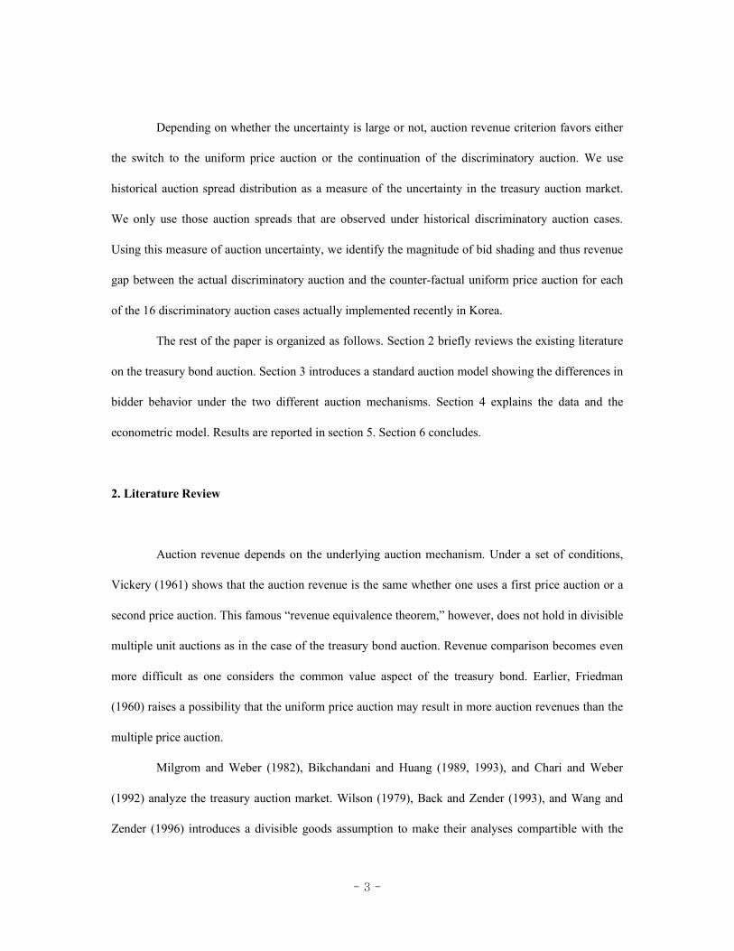
Figure 1 illustrates how the equilibrium cut-off yield spread is determined using the micro-

level bidding data on the discriminatory auction which occurred on July 18, 2000. (A full set of micro

level bidding data is available upon request.)

- 9 -

Figure 1: Market demand function and cut-off price

(discriminatory price auction on July 18, 2000)

-7

-6

-5

-4

-3

-2

-1

0

1

2

3

4

5

6

7

8

9

0 20 40 60 80 100 120 140 160 180 200 220 240 260 280 300

demanded quantity (%)

yiel

d sp

read

(bp)

cut-off price

Now, suppose that you have derived individual demand functions under the counter-factual

uniform price auction. Let nii ps ,,1)}({ = be a collection of such counter-factual demand functions

constructed for each individual who has participated in the discriminatory auction. (Here we are

implicitly assuming that bidder composition does not change as the auction mechanism changes,

which assumption sounds a bit strong. We will revisit this issue later.) By summing the individual

demand functions, we have the market demand function, say ∑=

=n

ii pspS

1)()( . Under the

hypothetical uniform price auction, the market clearing price would have been determined as the

minimum price among the elements of jp ’s in the set }1)(|{ ≥jj pSp .

In sections 2.2 through 2.4, we would like to characterize )( pbi and )( psi , and their

- 10 -

relationship. This relationship will turn out most important when comparing auction revenues later on.

3.2. Discriminatory price auction

Assume that individual bidders enjoy private values from the treasury bonds, that the private

values are not affiliated (Milgrom and Weber 1982), and that individual bidders do not strategically

interact. Let )(1 qdi− be the marginal value to bid i arising from securing one additional share of

the Treasury bond when she has already secured q . Under the assumptions, we neither put any

functional form restrictions across different )(1 qdi− ’s nor solve the individual bidding behaviors

considering strategic interactions (the same setting as in Lengwiler 1998, for example).

Consider the “price” of a treasury bond (with face value of one) which pays coupons at the

prevailing yield. Let d be the duration of the bond and p the yield using one basis point (=10-4) as

the measurement unit. (The same p now denotes yields, not the yield spreads. Here we are

obviously abusing notations for the purpose of notational simplicity.) Using a linear approximation,

we can approximate the bond’s price as “ 4101price −××−= jpd .”

Bidder i determines the optimal bidding strategy 1, ,{ ( )}ij i j j kb b p == to maximize the

expected profit

∑ ∑∫=

−=

−−

−−−

k

jijij

j

jj

b

ijbbbbpddqqdf ij

iki 11''

1''

4

0

1

,,)()101()(max

1

,

where '4

' 101price jj pd−−= , 1''' −−= ijijij bb∆ , 00 =ib and “no rationing at the margin” are used.

In fact, this optimization is a bit different from the treasury auction practices in Korea where

participants are allowed only up to a maximum of 5 bids which are in general smaller than k . We do

- 11 -

not think ignoring this difference would bias our empirical results. See Appendix Table A1 for the

number of bids per bidder.

By solving the k first-order conditions, we have

∑+=

+− −=−

k

jjjjjjijij fpppbdf

1''

*1

**1 )(])([ ⇔ )]1/1)(([ *1

** −−+= + jjjjiij hpppdb ,

where we have used (i) )/( kjjj fffh ++= , (ii) 0≠jf , and (iii) the definition of

jj pdp 4* 101 −−= . Note that the general solution takes the form )()( **jjijiij pdpbb δ+== with

0)1/1)(( *1

** ≥−−= + jjjj hppδ .

Not to cause confusion to the readers, let us comment on the usage of notations in the rest of

the paper. We are moving back and forth between the unit bond prices and the bond yields.

Measurements in terms of unit bond prices are denoted with an asterisk (*), and measurements in

terms of bond yields are denoted without an asterisk. For example, *jp and *

jδ are measured in

bond prices, whereas jp and jδ (as to be defined shortly) in bond yields.

The solutions allow nice economic interpretations. First, we observe that individual bidders

shade their bids in the sense that their actual bids are smaller than the “truth-revealing” bids,

)()()( ***jijjiji pdpdpb ≤+= δ . As is well known, the reason for bid shading here under the

discriminatory price auction is essentially the same as bid shading in the first price sealed bid auction.

What is less well known is that it is also similar to “shirking” in a typical principal-agent

model. The solution has exactly the same form if you map bidding to effort level, and cut-off yield

distribution to agent type distribution. “What you pay” is the bidding yield in the case of the

discriminatory auction and the effort level in the case of agent models. “What you get,” however, is

not exactly one for one. Rather a fraction of what you pay, resulting in bid shading and effort shirking.

Under the discriminatory auction, if a bidder believes that she still has a chance to secure an additional

- 12 -

share of the bond, she faces an incentive to under-bid, that is, to shade. To save on payment, she bids

less so far as chances are there, resulting in bid shading.

Second, only at kp shading does not occur, )()()( ***kikkiki pdpdpb =+= δ since 1=kh

and thus 0* =kδ . According to the belief about the cut-off yield, you have already reached the

maximum possible yield level at kp . There is absolutely no chance that the market clearing yield

further goes up passing kp Knowing this, bidders face no incentive to shade. Bidder i submits a

bid if she wants an additional share in the sense that *1 )( ki pqd ≥− , and not otherwise, leading her to

bid )( *ki pd at kp . At each “candidate” yield level, the bidder ask herself, “Would the ascending

auction further go up?” If the answer were positive, she would shade. Otherwise, she would reveal the

truth.

Third, shading depends on your belief about the market clearing yield level. As well known

in the literature, there exists one-to-one relationship between ),,( 1 khh and ),,( 1 kff . Let me

explain this relationship using the previous example of ascending auction. For the market clearing

yield to be determined at level jp , the ascending auction process should not have stopped at each of

the previous yield levels 1p through 1−jp , and then it should stop immediately at the current yield

level jp . Thus, the probability that the market clearing yield will be jp is the product of the initial

marginal probability and the subsequent conditional probabilities, leading to

jjj hhhf ⋅−⋅⋅−= − )1()1( 11 .

Again, imagine that you are attending an ascending yield auction and that you are now at

“node” jp . Based on your belief, if you are sure that the yield will be determined at the current level

and thus you are in the terminal node )( kj = , then you face no incentive to shade. On the other hand,

- 13 -

if you believe that the current node may not be the terminal node with positive probability )( kj < ,

you face an incentive to save money by under-bidding, that is, by bid-shading.

To shade or not, and how much to shade if you do, really depends on the relative strength of

these two opposing forces. At jp , you believe that this yield is the market clearing level with strength

proportional to jf , and you believe that this yield will further go up with strength proportional to

kj ff +++1 . The relative strength of these two forces is nothing but jkjj fffh /)(1/1 1 ++=− + .

As you see from the equilibrium bidding function )()( **jjiji pdpb δ+= , the amount of shading

)()( ***jjiji pdpd δ+− is increasing in *

jδ , which is equal to )1/1)(( *1

* −− + jjj hpp , and thus

increasing in 1/1 −jh and decreasing in jh .

At each yield level, say jp , the degree of shading really depends on jh , which is the hazard

rate at that yield level. This hazard measures the strength with which you believe that the market

clearing yield will be determined at the current level without going up any further (conditional on that

the auction process has already reached that level). Shading would be depressed as you believe more

strongly that the current level is the final node, and it would be encouraged as you believe more

strongly that the market clearing yield would further go up.

3.3 Uniform price auction

Unlike in the discriminatory auction, you do not pay what you bid. Rather, you pay what

other participants bid “at the margin.” This aspect of the uniform price auction is quite similar to the

second price sealed bid auction, resulting in “truth revealing” in both cases. The Korean treasury

auction market is highly competitive as there are many market participants and as none of them has

- 14 -

dominant market power. A bidder believes that she can influence neither other bidders’ bidding

behaviors nor the market clearing price, a reasonable description of the Korean treasury auction

market.

At all yield levels, bidders now do not face any incentive to shade. Bidder i bids if she

wants an additional share in the sense that *1 )( ji pqd ≥− , and not otherwise, leading her to bid

truthfully )( *ji pd at jp . Recall that in the case of the discriminatory auction, bidders only reveal

the truth when they are 100% sure that there is absolutely no chance that the market clearing yield will

further increase (that is, only at level kp ). Now, in the case of the uniform price auction, bidders

reveal truth at all price levels kpp ,,1 .

Of course, we can verify the above heuristics by formally solving the bidders’ optimization

problem. Let sp be the market clearing yield under the uniform price auction. Bidder i determines

the optimal bidding strategy, say 1, ,{ ( )}ij i j j ks s p == to maximize the expected profit.

∑ ∫=

−−

−−=

k

jijj

s

ijs

ssspddqqdpp ij

iki 1

4

0

1

,,)101()()Pr(max

1

,

where “ 41 10 jd p−− ,” say *jp , is again the unit bond price corresponding to the yield level of jp .

By solving the first-order conditions, we have

[ ] 0)()Pr( *1 =−= −jijij

s psdpp ⇔ )( *jiij pds = for all kj ,,1= .

Note that the solution takes the form )()( *jiji pdps = , kj ,,1= , that beliefs about the market

clearing yield do not play any role, that bidders always reveal truth, and that there arises no shading at

any yield level.

- 15 -

3.4 Recovering uniform price bidding from discriminatory price bidding

Through the above two sub-sections, we have characterized the equilibrium bidding

strategies under each of the discriminatory auction and the uniform price auction. Bidders shade their

bids under the discriminatory auction, whereas they do not under the uniform price auction. The

degree of shading is determined by the bidders’ belief about the market clearing yield under the

discriminatory auction.

Once we identify the bidders’ common belief about the market clearing yield under the

discriminatory auction, then we can recover their counter-factual bidding functions under the uniform

price auction.

In the foregoing sub-sections, by implicitly assuming that bidder composition does not

change as the auction mechanism changes, we have not addressed an important issue whether the set

of auction participants grows or shrinks. It is arguably agreed that auction participants increase under

the uniform price auction. It is because the uniform price auction is more friendly to individual

participants in that individuls when making bids do not have to worry about the uncertainty in the cut-

off yield level. Individuals are more likely to join the treasury auction (of course, through their

primary dealers) under the uniform price auction mechanism. If that is the case, our analysis, by

assuming that auction participants do not change, would underestimate the market demand under the

uniform price auction, and thus underestimate the auction revenue increase resulting from switching to

the uniform price auction.

Using the results in sections 2.2 and 2.3, we derive the relationship.

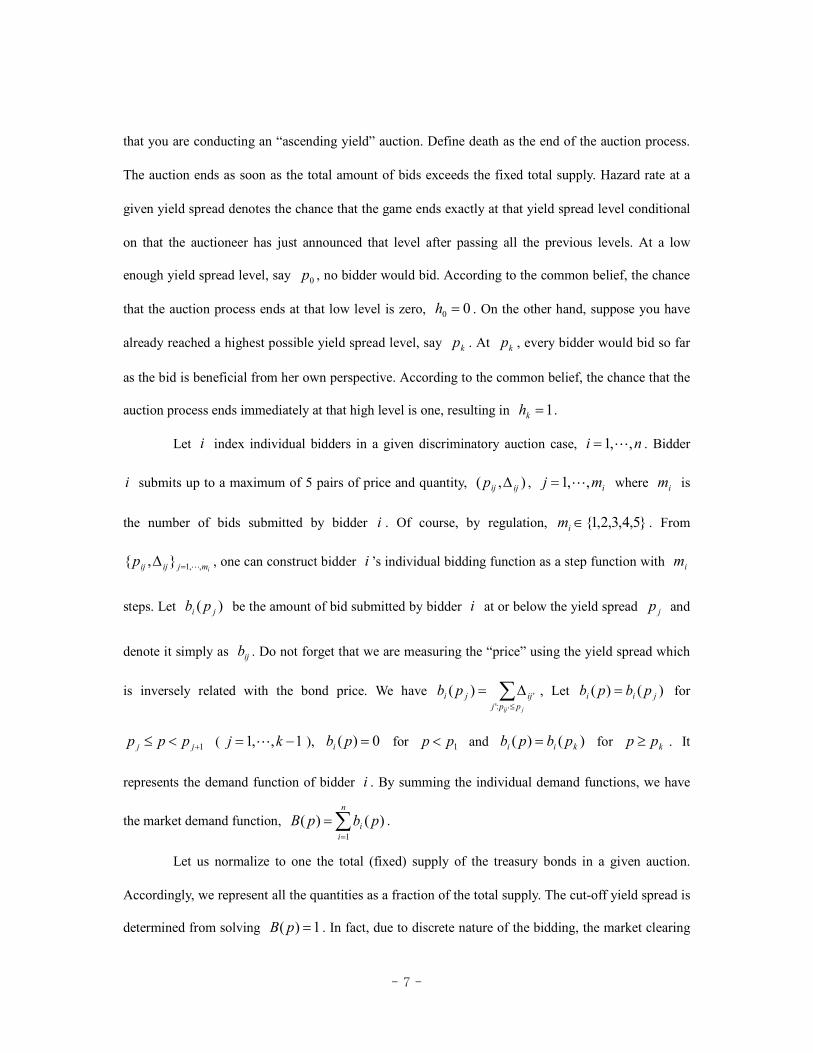
)()( **jjiji pdpb δ+= , )()()()( *

jjijijiji pbpspdps δ+=⇒= ,

where )1/1)(()/(10 1*4 −−== + jjjjj hppdδδ . Figure 2 shows this relationship.

- 16 -

Figure 2: Bidding functions: discriminatory vs uniform

From the relationship, we observe that the degree of shading can be represented in two

alternative terms: either by *jδ using bond prices as the measurement unit or by jδ using bond

yields as the measurement unit. Let me explain bid shading using the latter term. It is a product of the

following two terms. The first term, jj pp −+1 , measures how much you gain in terms of the bond

yield when you wait for another “node,” and the second term, 1/1 −jh , measures the relative strength

of your belief with which you believe you would reach the next node rather than “burst.”

Once we secure information on ),,( 11 −khh representing the bidders’ common belief about

the market clearing yield under the discriminatory auction, we can recover the counter-factual bidding

function )( psi from the observed bidding function )( pbi .

Let )5( ≤ii mm be the number of the bids submitted by bidder i in the discriminatory

Quantity demanded

yield

pk

O

si(pj)=bi(pj+δj)

pj

pj+δj

si(p) bi(p)

δj=(pj+1-pj)⋅(1/hj-1)

- 17 -

price auction, and },{ ijijp ∆ be those pairs, imj ,,1= , ni ,,1= . Of course, },,{ 1 kij ppp ∈

by construction. We have

∑+≤

∆=+=jjij ppjijjjiji pbpsδ

δ':'

')()(

It is the “derived” bidding function of bidder i under the counter-factual uniform price auction. By

summing the individual demand functions, we can also derive the hypothetical market demand

function, ∑=

=n

jjij pspS

1)()( .

The market clearing price will be determined as the minimum jp among the elements of

the set ∑=

≥=n

ijijj pspSp

1}1)()(:{ . Once we compute the market clearing price, we can compute

the auction revenue in the hypothetical uniform price auction. Thus, we can compute the percentage

auction revenue increase which one enjoys by switching the auction mechanism from the

discriminatory auction to the uniform price one.

Depending on the amount of uncertainty regarding the market clearing yield spread, it may or

may not pay to switch to the uniform price auction from the discriminatory one. It is an empirical issue

after all.

4. Data, Econometric Model

The data are micro-level, individual bidding data for the recent discriminatory auction cases

held in the Korean treasury auction market. Table 1 shows basic characteristics of each auction

analyzed in this paper. Out of a total of 16 cases in the sample, 10 are taken consecutively from

September 6, 1999 to January 10, 2000, and the remaining 6 from May 15, 2000 to July 18, 2000.

During the in-between period, discriminatory auctions were used with variable supply. Variable supply

- 18 -

itself would make bidders shade. Not to confound the effect of discriminatory/uniform price auctions

with the effect of fixed/variable supplies, we exclude these interim auction cases with variable supply.

Table 1: Background information on each of 16 discriminatory auctions

auction date cut-off yield

(bp)

market yield

(bp)

maturity

(year)

duration

(year)

total supply

(billion won)

19990906 865 850 1.00 0.97 1195.16

19990913 944 930 2.65 2.65 1196.19

19990928 989 975 4.01 4.01 790.40

19991004 839 836 1.00 0.97 1164.90

19991011 841 837 2.68 2.68 1357.40

19991018 938 939 4.05 4.05 798.30

19991108 811 807 1.00 0.97 776.30

19991115 838 832 2.68 2.68 1184.90

19991206 870 869 2.67 2.67 349.80

20000110 906 902 1.00 0.97 738.67

20000515 929 929 3.79 4.05 279.60

20000605 823 828 1.00 0.97 287.20

20000612 865 863 2.51 2.67 578.70

20000619 902 901 3.79 4.05 767.90

20000710 795 790 2.45 2.67 586.00

20000718 815 816 4.07 4.16 778.00

From the discussions in section 2, we readily notice that the whole revenue comparison boils

down to an issue of estimating uncertainty surrounding the market clearing yield spread. One may

think of several approaches. First, use an empirical distribution of the historically observed yield

spreads under the 16 discriminatory auction cases. Yield spreads are defined as the differences

between the observed cut-off yields and the yields in the secondary market at morning of the auction

date.

The first approach is simple, but naive. Market clearing yield spreads may depend on a

- 19 -

number of variables. Here comes the second approach. Second, use a more sophisticated method. For

this purpose, run a multiple regression of the yield spread, defined as the cut-off yield minus the

secondary market yield, on a constant, maturity dummies, year dummies, number of bidders, and the

auction size (face value).

Once you estimate the regression coefficients (reported in Appendix Table A2), compute the

16 residual terms (graphed in Appendix Figure A1). Then, we approximate the yield spread

distribution as the empirical distribution function of these 16 residuals, shifted to the right by a

relevant regression function. The regression function is obtained by combining the coefficient

estimates with the current auction characteristics. We use this sophisticated approach in this paper.

(The results were basically the same when we alternatively used the empirical distribution of the yield

spreads historically observed, shifted to the right by the current secondary market yield.)

Given the historically observed yield spreads, we would like to estimate ),,( 11 −= khhh .

For this purpose, let )16()1( pp ≤≤ be those 16 realizations of the yield spread, that is, the 16

residuals shifted to the right by the regression function. We measure them using 1 basis point as the

measurement unit after approximating them upto the nearest integer values. Let k be the number of

the distinctive elements among the )( jp ‘s. Let us take these distinctive elements as },,{ 1 kpp , the

support set of the market clearing yield spread. Let 11 ,, −kff be the empirical frequencies of

)( jp ‘s which are equal to 11 ,, −kpp . We estimate ),,( 11 −= khhh using )/( kjjj fffh ++= ,

1,,1 −= kj .

Often, it is tempting to impose monotonicity on ),,( 11 −= khhh that 11 −≤≤ khh holds.

Imposing this monotonicity assumption is useful for the following two reasons. First, it will smooth

out the empirical hazard estimates. Second, it is a priori reasonable to assume that the hazard rate of

the “ascending yield” auction increases as the yield spread level further goes up.

- 20 -

Estimating the empirical hazard rates under this assumption is easy using the so called

“moving to the right” idea. Let us explain this idea. You first estimate jh ’s as above,

)/( kjjj fffh ++= . If the estimated hazard rates satisfy the monotone hazard property, stop. If

not, search for the yield spread level sequentially from the lowest where the monotonicity breaks down

for the first time. Let jp be such level, that is, jj hhh >≤≤ −11 . You move one observation

observed at 1−jp to the right such that it behaves as if it were observed at jp . As a result of this

“moving to the right,” 1−jf decreases by one whereas jf increases by one. Accordingly, 1−jh

decreases whereas jh increases. Repeat this moving to the right procedure until you have jj hh <−1 .

When the above step is over, you might have disturbed the previously holding inequality. If

you happen to see 12 −− > jj hh , you move one observation observed at 2−jp two steps to the right

such that it behaves as if it were observed at jp . Moving one step to the right to 1−jp , would cause

jj hh >−1 , so this move is ruled out. As a result of this “moving to the right,” 2−jf decreases by one

whereas 1−jf stays the same and jf increases by one. Repeat this “moving to the right” until you

have jjj hhh ≤≤ −− 12 .

When the above second step is over, you might have disturbed the previously holding

inequality. If you happen to see 23 −− > jj hh , you move one observation observed at 3−jp to the right

such that it behaves as if it were observed either at 1−jp or at jp . Think again why moving to 2−jp ,

one-step to the right, is ruled out. (It is because it would have caused 12 −− > jj hh .) Repeat this

procedure until jjjj hhhh ≤≤≤ −−− 123 holds. In this process, note the following two points. First, in

- 21 -

a given move, you do not want to move further to the right unless necessary. In the previous step, you

would stop moving at 1−jp rather than further advancing to jp unless needed. Second, you stop the

process of moving to the right immediately when you have jhh ≤≤1 .

Then, you search for a new yield spread at which the monotonicity breaks down (again for

the first time), and repeat the whole procedures as explained above. Finally, you have 11 −≤≤ khh .

As we have mentioned above, these hazard estimates are advantageous in that they are smoother, and

that they satisfy an a priori appealing monotonicity property.

So far we have explained an approach to deriving the common belief about the cut-off yield

level. Other approaches include (i) introducing GARCH type models into the error terms in the above

regression approach, and (ii) estimating the yield spread distribution using information contained in

the yields themselves and/or interest derivative products. Adding GARCH idea to the above procedure

should be easy. Extracting additional information from the interest derivative products, should be a bit

involved.

For a given discriminatory auction case, once you estimate the percentage revenue difference,

you want to compute its sampling error. There are two sources of the sampling error. One is the

uncertainty arising from estimation of the yield spread distribution. The other is the uncertainty arising

from who participate in a given auction.

First, recalling that we have estimated this distribution using the 16 cases, we would like to

measure this uncertainty by applying Bootstrap re-sampling techniques to those 16 cases. More

concretely, out of 16 integers, 1 through 16, you select a set of 16 numbers through random sampling

with replacement. Then, by using the auction cases corresponding to these 16 selected numbers, you

re-estimate the yield spread distribution. Using the re-estimated spread distribution, re-estimate the

percentage revenue difference. Then, repeat the whole procedures. This way, you can generate as

- 22 -

many percentage revenue differences as you wish.

Second, given an estimate of the yield spread distribution, it is the set of the participating

individual bidders who determine the percentage revenue difference. We also would like to address

this second source of uncertainty by using the Bootstrap re-sampling techniques. We will re-sample

the same size of the bidders from the original set of the bidders through sampling with replacement.

More concretely, out of integers, 1 through n , you select a set of n numbers by sampling randomly

with replacement. Then, by using the bidders corresponding to these selected numbers, you re-estimate

the percentage revenue difference. Then, repeat the whole procedures. This way, you can generate as

many percentage revenue differences as you wish.

To sum, we can measure the sampling uncertainty using the Bootstrap re-sampling techniques.

There are two sources of sampling uncertainty. One type of uncertainty lies in estimating the yield

spread distribution. The other, in sampling (drawing) individual bidders. Of course, we want to

consider both sources of uncertainty jointly as well as separately.

To address both sources of uncertainty, you apply the re-sampling scheme at both stages. In a

single run, you first re-sample the 16 auction cases. Estimate the yield-spread distribution. Re-sample

the set of bidders. Then, finally by combining the estimated yield distribution with the set of re-

sampled bidders, you come up with an estimate of the percentage revenue difference. Repeat the

whole procedure as many times as you wish.

To address only the uncertainty in the yield spread estimates, you only apply the re-sampling

scheme at the first stage. In a single run, you first re-sample the 16 auction cases. Estimate the yield-

spread distribution. (Use the original set of bidders. Do not apply re-sampling at the second stage.)

Then, by combining the estimated yield distribution with the set of the original bidders, you come up

with an estimate of the percentage revenue difference. Repeat the whole procedure as many times as

you wish.

- 23 -

Finally, to address only the uncertainty in the set of the participants in the auction, you only

apply the re-sampling scheme at the second stage. (Use the 16 historically observed yield spreads to

estimate the yield spread distribution. That is, do not apply re-sampling at the first stage.) In a single

run, you use the yield-spread distribution estimated from the original 16 auction cases. You stick to

this estimate throughout the replications. Only re-sample the set of bidders. Then, by combining the

original yield distribution with the set of re-sampled bidders, you come up with an estimate of the

percentage revenue difference. Repeat the whole procedure as many times as you wish.

5. Results

The Korean treasury auction market is highly competitive as there are 30 potential

participants none of whom possesses dominant market power. Short squeeze does not arise as there is

no “when-issued market” in the Korean treasury auction market. Lack of when-issued markets, though,

increases uncertainty facing the cut-off price.

Tables 2 to 4 show the estimation results obtained under monotonicity assumption imposed

on the hazard etimates. Results obtained without imposing the monotonicity assumption, are basically

the same (available upon request). The auction carried out on Dec. 6, 1999 is much smaller in size.

The results are basically the same whether we include or exclude this case. Also, regarding those 6

discriminatory auction cases carried out between May 15, 2000 and July 18, 2000, our results are

robust to inclusion/exclusion of these cases.

Our empirical results show that uniform price auctions, had they been implemented, would

have increased auction revenues during the sample period when the Korean government in fact used

discriminatory auctions. Judging from Bootstrap re-sampling standard errors, we have established

evidences that the uniform price auction, had it been adopted in Korea back in the years 1999 and

- 24 -

2000, would have increased auction revenue for 11 cases out of a total of 16 cases with an average of

0.13 % revenue increase.

To sum, the uniform price auction is revenue enhancing in the Korean treasury auction

market, and thus the Korean government’s switch to the uniform price auction in August 2000 was a

right policy choice.

Table 2: Percentage revenue difference between discriminatory and uniform auctions

(both yield-spreads and bidders re-sampled; monotone hazard imposed)

Auction

Date Mean(%) Median(%) SE(%)

maximum

(%)

minimum

(%)

19990906 0.05 0.05 0.02 0.10 -0.10

19990913 0.15 0.15 0.06 0.31 -0.25

19990928 0.36 0.38 0.09 0.54 -0.23

19991004 0.00 0.00 0.00 0.01 0.00

19991011 0.00 0.00 0.00 0.01 0.00

19991018 0.00 0.00 0.01 0.12 0.00

19991108 0.03 0.03 0.01 0.05 -0.01

19991115 0.05 0.05 0.01 0.09 0.00

19991206 0.05 0.02 0.08 0.33 -0.32

20000110 0.06 0.06 0.01 0.07 -0.05

20000515 0.31 0.32 0.04 0.41 0.11

20000605 0.00 0.00 0.00 0.02 0.00

20000612 0.09 0.09 0.03 0.17 -0.06

20000619 0.13 0.14 0.02 0.19 0.00

20000710 0.18 0.18 0.03 0.24 -0.07

20000718 0.07 0.07 0.03 0.17 0.00

Table 3: Percentage revenue difference between discriminatory and uniform auctions

(only yield-spreads are re-sampled; monotone hazard imposed)

auction

date Mean(%) Median(%) SE(%)

maximum

(%)

minimum

(%)

- 25 -

19990906 0.04 0.05 0.02 0.06 -0.10

19990913 0.15 0.16 0.03 0.17 -0.20

19990928 0.37 0.39 0.08 0.45 -0.22

19991004 0.00 0.00 0.00 0.00 0.00

19991011 0.00 0.00 0.00 0.00 0.00

19991018 0.00 0.00 0.00 0.00 0.00

19991108 0.03 0.03 0.01 0.03 0.00

19991115 0.05 0.04 0.01 0.06 0.00

19991206 0.02 0.02 0.00 0.03 0.00

20000110 0.06 0.06 0.01 0.06 -0.05

20000515 0.30 0.32 0.04 0.41 0.12

20000605 0.00 0.01 0.00 0.01 0.00

20000612 0.08 0.09 0.02 0.11 -0.01

20000619 0.13 0.14 0.02 0.20 0.00

20000710 0.18 0.19 0.02 0.22 -0.01

20000718 0.07 0.08 0.02 0.10 0.00

Table 4: Percentage revenue difference between discriminatory and uniform auctions

(only bidders are re-sampled; monotone hazard imposed)

auction

date Mean(%) Median(%) SE(%)

maximum

(%)

minimum

(%)

19990906 0.03 0.04 0.01 0.06 0.00

19990913 0.17 0.16 0.04 0.32 0.08

19990928 0.40 0.40 0.04 0.51 0.29

19991004 0.00 0.00 0.00 0.02 0.00

19991011 0.00 0.00 0.00 0.01 0.00

19991018 0.00 0.00 0.01 0.10 0.00

19991108 0.03 0.03 0.01 0.05 0.02

19991115 0.06 0.06 0.01 0.09 0.03

19991206 0.06 0.02 0.08 0.40 0.00

20000110 0.06 0.06 0.00 0.08 0.04

20000515 0.33 0.32 0.01 0.37 0.32

20000605 0.01 0.01 0.00 0.02 0.00

- 26 -

20000612 0.10 0.10 0.02 0.17 0.02

20000619 0.15 0.14 0.01 0.18 0.12

20000710 0.19 0.19 0.01 0.24 0.16

20000718 0.09 0.09 0.03 0.19 0.02

6. Concluding Remarks

In this paper, we compare auction revenues across the two different auction mechanisms,

discriminatory vs uniform price auctions, using a structural approach. The auction revenue difference

critically depends on the hazard function estimates of the market clearing yield. We have estimated the

hazard rates using the historically observed auction yield data, adjusted for several factors such as

secondary market rates, maturities, years, number of participants, and the auction size. Using these

historical data set, we estimate the hazard rates with and without imposing the monotone hazard

assumptions. We believe that monotone hazard property makes senses, and that imposing it reduces

the sampling uncertainty.

We measure sampling uncertainty using the Bootstrap re-sampling methods. We address the

sampling uncertainty arising from the hazard estimates as well as the sampling uncertainty arising

from who joins the auction. We address these two types of uncertainty separately as well as jointly.

This paper theoretically has clarified the role of the hazard rates in the discriminatory auction

by comparing it to a typical principal agent model, and empirically has offered new ways of estimating

the hazard rates. This paper has also suggested the use of Bootstrap re-sampling techniques to address

sampling uncertainty from two different sources. Using the re-sampling method, we can identify these

two types of uncertainty separately.

This research leaves room for improvements, though. As the auction scheme changes,

- 27 -

participants may change. For example, as the auction mechanism switches from the discriminatory

auction to the uniform price one, it is expected that more would participate in the auction. If so, our

analyses based on “no change” assumption of the participants, would underestimate the revenue

increase resulting from the switch. In this paper, as we have obtained such results that the uniform

price auction increases the auction revenue under the “no participant change” assumption, our results

would only have been strengthened if we had considered auction participation decision as well.

This paper has not formally considered the auction participation decision. Theoretical as well

as empirical analyses of the auction participation decision, would be interesting, and are left for future

research.

In this paper, we have assumed that all the auction participants have the same belief about the

market clearing cut-off yields, and additionally that this belief is well approximated by the distribution

of the historically observed cut-off yields once adjusted for factors like secondary market rates,

maturities, years, number of participants, and the auction size. It would be interesting to see how the

results change as one uses different distributions.

In this paper, we have explained how to recover bidding functions under the uniform price

auction from those under the discriminatory price auction. One can apply the similar techniques to

solve the reverse problem, that is, to derive bidding functions under the discriminatory auction from

those under the uniform price auction. As the Korean government has switched to the uniform price

auction from August 2000, we can also compare auction revenues across different auction mechanisms

using the observed uniform price auction data. These results will be reported in a separate paper.

Using micro-level auction data, one can potentially think of three different approaches to

measuring the percentage revenue difference between the uniform price and the discriminatory

auctions.

First, “discriminatory to uniform.” This is an approach we have adopted in this paper. Given

- 28 -

individual bids under the discriminatory auction, we recover individual bids under the counter-factual

uniform price auction.

Second, “uniform to discriminatory.” Given individual bids under the uniform price auction,

we recover individual bids under the counter-factual discriminatory auction.

Third, we can compare historically observed auction revenues (or auction cut-off yields) from

two different auction mechanisms. For this purpose, one may simply run a multiple regression of

(auction revenue/face value) (or auction cut-off yield) on a constant, uniform price auction dummy,

maturity dummies, year dummies, number of bidders, auction size, and the secondary market yield.

Then, test the statistical significance of the coefficient of the uniform price auction dummy. If it turns

out positive and statistically significant, then the uniform price auction is more revenue enhancing

relative to the discriminatory auction and vice versa. (The opposite is true if one uses the cut-off yield

as the dependent variable in the regression).

Among the three approaches, the first two are structural in nature in the sense that one has to

use a theoretical model to derive the counter-factual individual bids from the observed ones. The third

is purely statistical and reduced-form in nature in the sense that one does not need any theoretical

model.

In terms of data requirement, the first two are less demanding as they only require data from

one auction mechanism, discriminatory or uniform price. The third requires data from both auction

mechanisms. In terms of “statistical control,” the first two approaches are advantageous. It is because,

in the first two approaches, an auction case is compared to itself, eliminating the need for statistical

control. However, the first two approaches critically depends on the theoretical model used and also on

the empirical estimates of the cut-off yield distribution.

In the third approach, one discriminatory auction is compared with another uniform price

auction. These two auctions are different not only in terms of the auction mechanism but also in many

- 29 -

other aspects such as maturities, years, number of bidders, auction sizes, secondary market rates at

morning of the auction day, interest rate expectations, yield uncertainties, financial and macro shocks,

and many other factors. Observable differences are controlled to a certain extent by including them as

regressors in the multiple regression equation. However, it is simply impossible to control even the

major differences in an adequate way, let alone all the differences.

We leave it as a future research to compare revenue differences across these three different

approaches. Specifically we would like to address issues like (i) whether results from the structural

approaches and results from the reduced-form approach would agree, and (ii) whether the two

structural approaches would yield mutually consistent results.

- 30 -

References

[1] Back, K and J. Zender (1993), "Auctions of divisible goods : On the rationale for the Treasury

experiment," Review of Financial Studies, vol. 6, 733-764.

[2] Bank of Korea (2000), “The Korean Treasury Bonds Market: Future Prospects and Current

Tasks” (in Korean).

[3] Bikchandani, S., and C. Huang, (1989), “Auctions with Resale Markets: An Exploratory Model

of Treasury Bill Markets,” Review of Financial Studies, vol. 2, 311-339.

[4] Bikchandani, S. and C. Huang (1993), “The Economics of Treasury Securities Markets,”

Journal of Economic Perspectives, vol. 7, 117-134.

[5] Cammack, E.B. (1991), “Evidence on bidding strategies and the information in Treasury bill

auctions,” Journal of Political Economy, vol. 99, 100-130.

[6] Chari, V. and R.J. Weber (1992), "How the U.S. Treasury Should Auction Its Debt," Federal

Bank of Minneapolis Quarterly Review, vol. 16, no.4.

[7] Chatterjea, A. and R. J. Jarrow (1998), "Market Manipulation, Price Bubbles, and a Model of

the U.S. Treasury Securities Auction Market," Journal of Financial and Quantitative Analysis,

vol. 33(2), 255-289.

[8] Cottarelli, C. (1997), “Treasury Bill Auctions: Issues in Design,” in Coordinating Public Debt

and Monetary Management(IMF), 190-208.

[9] Dattels, P. (1997), “Microstructure of Government Securities Markets”, in Coordinating Public

Debt and Monetary Management(IMF), 209-282.

[10] Feldman, R.A. and R. Mehra (1993), “Auctions: Theory and Applications,” IMF Staff Papers,

No.40, 485-511.

[11] Friedman, M. (1960), A Program for Monetary Stability, 1959, NY : Fordham University Press.

- 31 -

[12] Goldreich, D. (1998), “Underpricing in Treasury Auctions,” IFA Working Paper 263, London

Business School.

[13] Gray, S. (1997), “Government Securities : Primary Issuance,” in Handbooks in Central Banking,

Bank of England.

[14] Heller, D. and Y. Lengwiler(1998b),"The Auctions of Swiss Government Bonds : Should the

Treasury Price Discriminate or Not ?", FRB.

[15] Hortacsu, A. (2002a), “Mechanism Choice and Strategic Bidding in Divisible Good Auctions :

An Empirical Analysis of the Turkish Auction Market.”

[16] Hortacsu, A. (2002b), “Bidding Behavior in Divisible Good Auctions: Theory and Evidence

from the Turkish Treasury Auction Market.”

[17] Kim, Gyung-Rok (2001), “The Impact of the Treasury Bonds Auction Techniques on the

Auction Revenue: In the Case of the Korean Treasury Bonds Auction Market,” Ph.D.

dissertation, Dept of Economics, Seoul National University (in Korean).

[18] Jegadeesh, N. and Y. Hamao (1997), “An analysis of Bidding in the Japanese Government Bond

Auctions,” Working Paper.

[19] Kroszner, R. (1993), An International Comparison of Primary Government Securities Markets,

Working paper, University of Chicago, Jan. 1993.

[20] Lee, S., Y. Ghaugh, K. Oh, A. Fayolle (1999), “Issuing and Managing the Treasury Bond,”

World Bank FCRA Project (in Korean).

[21] Lengwiler, Y. (1998), “The Multiple Unit Auction with Variable Supply”, FRB.

[22] Malvey, P.F. and C.M. Archibald (1998), Uniform-Price Auctions: Update of the Treasury

Experience. U.S. Treasury.

[23] Milgrom, P. and R.J. Weber (1982), “A Theory of Auctions and Competitive Bidding,”

Econometrica 50, 1089-1122.

- 32 -

[24] Ministry of Finance and Economy (1999), “Rules Governing Primary Dealers in the Korean

Treasury Bonds Auction Market,” The Korean Government (in Korean).

[25] Nautz, D. (1995), "Optimal bidding in multi-unit auctions with many bidders," Economics

Letters, vol. 48 301-306.

[26] Nyborg, K. G. and Sundaresan, S. (1996), "Discriminatory versus Uniform Treasury Auctions :

Evidence from When-Issued Transactions," Journal of Financial Economics, vol. 42(1), 63-104.

[27] Simon, D.P. (1994), "Markups, quantity risk, and bidding strategies at Treasury coupon

auctions," Journal of Financial Economics, vol. 35, 43-62.

[28] Umlauf, S.R. (1993a), “An Empirical study of the Mexican Treasury bill auction,” Journal of

Financial Economics, vol. 33, 313-340.

[29] Umlauf, S.R. (1993b), “Information Asymmetries and Security Market Design: An Empirical

Study of the Secondary Market for U.S. Government Securities,” Journal of Finance, vol. XLVI,

929-953.

[30] Vickery, W. (1961), "Counter-speculation, Auctions, and Competitive Sealed Tenders," Journal

of Finance, 16, 8-37.

[31] Viswanathan, S. and J.D. Wang (1998), "Auctions with When-Issued trading: A Model of the

U.S. Treasury Markets," U.S. Treasury.

[32] Wang, J. J. D. and J. F. Zender (1996), "Auctioning Divisible Goods," Working Paper,

University of Utah.

[33] Wilson, R. (1979), "Auctions of Shares," Quarterly Journal of Economics, 93, 675-689.

- 33 -

Appendix

Table A1 shows the average and the standard deviation of the number of bids per bidder for

each of the 16 discriminatory auction cases analyzed in this paper.

Table A1: Summary statistics on the number of bids per bidder

auction date

(yyyymmdd) average SD

19990906 3.16 1.37

19990913 3.89 1.12

19990928 3.30 1.44

19991004 3.58 1.24

19991011 3.83 1.36

19991018 3.96 1.25

19991108 3.60 1.39

19991115 3.85 1.23

19991206 1.73 0.79

20000110 3.75 1.27

20000515 2.00 1.13

20000605 1.96 1.11

20000612 2.95 1.32

20000619 2.13 1.26

20000710 2.60 1.29

20000718 3.58 1.47

16 auctions pooled 3.16 1.45

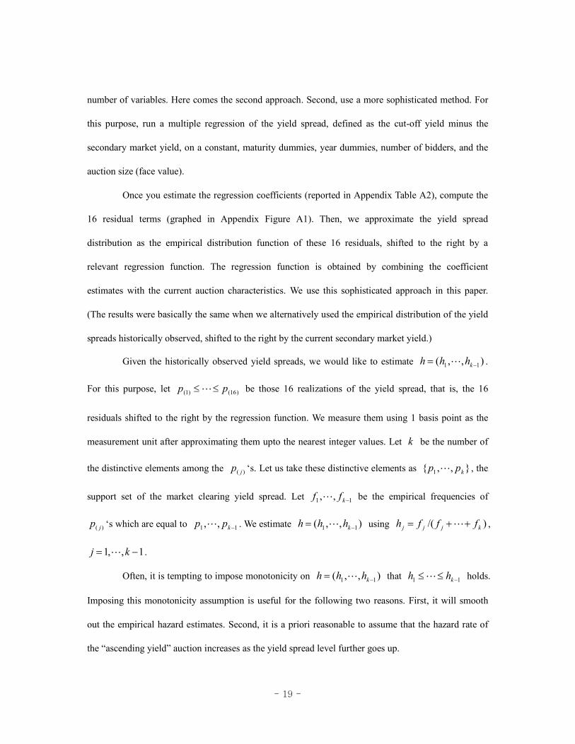
Table A2 shows the results of regressing the cut-off yield spreads on several covariates using

the 16 discriminatory auction data. Figure A1 is a histogram of the resulting residuals.

- 34 -

Table A2: Regression of the cut-off yield spread

explanatory variable coefficient estimate t-value

dmat=1 -1.32 -0.18

dmat=3 -0.56 -0.08

dmat=5 -1.67 -0.20

D2000 -3.46 -0.73

# of bidders 0.09 0.19

Auction size 0.00 0.65

regression equation: (cut-off yield spread) = α1(maturity 1 year dummy)+α2(maturity 3 year dummy)+α3(maturity 5 year dummy)+α4(auction year 2000 dummy)+α5(number of bidders)+α6(auction size)+(error)

Figure A1: Residuals from the cut-off yield spread regression