The Logistic Function Approach toDiscriminatory and Uniform Price

Treasury Auctions

Rasim Özcan∗

Abstract

There has been considerable debate in the literature concerning whether uniformor discriminatory pricing raise more revenue in Treasury Bill auctions. A standard ap-proach has been to examine empirically how revenue changes given a switch from onetype to the other. The weakness of this approach is that such a revenue change may bedue to changes in economic conditions. This paper is the first to examine the two meth-ods while taking into account changes in economic conditions. To do this, it adopts athree-stage procedure. First, it fits a logistic function to the cumulative bid distributionfor each auction. Second, it estimates two sets of equations relating the logistic functionparameters to economic conditions, one for uniform and one for discriminatory pricing,on the assumption that T-bill offerings by the government are exogenous. And third,using the estimated equations, it predicts how much revenue would have been raisedfrom discriminatory price auctions if instead uniform pricing had been used, holdingeconomic condition constant, and vice versa. The data employed are for Turkish Trea-sury auctions from 2000-2002, in the middle of which the Turkish Treasury switchedauction types. The results point to the superiority of the discriminatory price auction,but also cast doubt on the assumption that government T-bill offerings are exogenous.

Keywords: Treasury auctions, multi-unit auctions, discriminatory and uniform-price auctions, market bid, logistic functionJEL Classification Codes: D44, G18

∗Northwestern University, Department of Economics, 2001 Sheridan Road, Evanston, IL 60208-2600USA. Email: ozcanr@northwestern.edu. I am grateful to Richard Arnott, Ali Hortacsu, and Hideo Konishi.I thank to K. Ozgur Demirtas, Haldun Evrenk, and Bedri K.O. Tas for helpful discussions. I also thank tothe Central Bank of Turkey and the Istanbul Stock Exchange, both of which made this study possible byproviding the data. All errors are mine.

1 Introduction

In a multiunit auction problem, multiple units of identical objects are sold

through auctions. A typical example is that of Treasury bills, which are

sold by this method in many countries. There are two most commonly

used auction methods;1 discriminatory and uniform price auctions.2 In the

former, a bidder pay her bid amount if the bid is accepted. In the latter,

however, the minimum accepted bid, rather than the bid itself, is paid by

the bidder. Although both methods have been used for many years, there is

neither theoretical nor empirical consensus on which auction method raises

higher revenue.

A standard empirical approach in comparing the revenue raised from the

two auction types has been to compare how revenue changes given a switch

from one auction type to the other. The weakness of this approach is that

the change in revenue may be due to changes in economic conditions rather

than the change in auction type. This paper is the first to examine such

revenue changes while taking into account changes in economic conditions.

To do this, it adopts a three-stage procedure. First, it fits a logistic function

to the cumulative bid distribution for each auction. Second, it estimates

two sets of equations relating the logistic function parameters to economic

conditions, one for uniform and one for discriminatory pricing. And third,

using the estimated equations, it predicts howmuch revenue would have been

raised from each auction during the period when discriminatory pricing was

employed if instead uniform pricing had been employed, holding economic

conditions constant, and vice versa. To implement this procedure, it employs1A hybrid of these two methods used in Spain is beyond the scope of this paper.2 In both auction methods, bidders submit multiple price-quantity pairs, and then the

seller allocates the supply to those bid pairs whose price bid is higher than the minimumaccepted price bid.

2

Turkish treasury auction data for the period 2000-2002, in the middle of

which the Turkish Treasury switched auction types.

In the first part of the paper, by estimating the parameters of the logis-

tic growth curve for the Turkish Treasury auction data, I show that logistic

growth curves represent the market bid functions fairly well, a result con-

firmed in the literature for some other countries.3 In the second part of the

paper, I estimate the fluctuations in the parameters of the logistic function

from one auction to another by using economic variables like Preget and

Waelbroeck (PW) (2003) do for only discriminatory auctions. In addition

to finding the economic determinants of the estimated logistic function pa-

rameters under discriminatory auctions as do PW (2003), I show that this

can be also done for uniform auctions. I also find the estimation equations

for the parameters under uniform auctions. The estimation equations for

the parameters are different for the two auction methods. This suggests

that under different auction types bidders pay attention to different market

variables. Thus the approach used in this paper differs that of Boukai and

Landsberger (BL) (1999) and Berg, Boukai, and Landsberger (BBL) (1999),

who treat fluctuations in the parameters of the logistic function from one

auction to another as random shocks instead of estimating these fluctuations

from economic variables.

Estimating the logistic curves allows us to determine the results of both

auction formats under the same economic environment. The estimation

results are somewhat contradictory. According to the estimation results

with the discriminatory auctions data, discriminatory auctions raise much3Boukai and Landsberger (1999) show it for Israeli auctions data, Preget and Wael-

broeck (2003) for French data, and Berg, Boukai, and Landsberger (1999) for Norwegianand Swiss data. The first two studies show that the aggregate demand functions for dis-criminatory auctions can be well approximated by the logistic growth function. The lastone finds that the market demand function of Norwegian bonds — long-term bills — issuedwith uniform price auctions is also in the form of a logistic curve.

3

more revenue than uniform auctions. However, on the uniform auctions

data, the estimated revenue of discriminatory auctions is a little lower than

that of uniform auctions. This result might be due to two reasons. First, the

Treasury decides the optimal supply in an auction given the auction method,

so supply may vary in the two types. Second, the frequency of auctions is

also determined given the auction method. Both of these issues are left for

future study. In light of these results, I conclude that the discriminatory

format raises more revenue for the Treasury.

The data set employed in this paper is prepared in Ozcan (2004). It

contains bidder-level data for both discriminatory and uniform auctions un-

dertaken by the Turkish Treasury from January 2000 to February 2002. The

Turkish Treasury switched from discriminatory to uniform auctions in Feb-

ruary 2001. The data set also contains all the secondary market transactions

either done in the Istanbul Stock Exchange (ISE) Bonds and Bills Market,

or conducted through bilateral trade, which has to be registered to the ISE

Settlement and Custody Bank.

The findings of this paper appears contradictory to those of BBL (1999),

who argue in favor of uniform auctions. The approach taken here is superior

to theirs, since they don’t account economic conditions. Moreover, using both

auction methods during one time period, which is the case in BBL’s (1999)

data,4 is significantly different from using only one auction method for one

time period and the other method for another time period, which is the

case in this paper’s data. The strategic decisions of bidders might very well

be different under these two different auction environments. One thus may

naturally expect different comparative revenues for each auction method4In their data for Norwagian Treasury auctions, bills are the Treasury’s short-term

securities whereas bonds are the long-term securities. For a given time period, both short-and long-term securities co-exist in their data. Unlike the approach taken in this paper,they compare the Treasury’s revenue for short-term and long-term securities issued withdiscriminatory and uniform price auctions, respectively.

4

under these two distinct types of conditions. Therefore, the results of BBL

(1999) may not be directly comparable with the results of this paper.5

Among others, Wilson (1979), Nautz (1995), and Heller and Lengwiller

(1998) present theoretical studies in favor of uniform auctions. Back and

Zender (1993), Binmore and Swierzbinski (2000), and Wang and Zender

(2002) provide some of the theoretical studies in favor of discriminatory auc-

tions. Empirical studies also produce mixed results. For example, using U.S.

data Simon (1994a) finds that borrowing costs are lower in discriminatory

auctions. Adopting a structural approach to estimate nonparametrically a

symmetric private-values model for Turkish Treasury auctions data, Hor-

tacsu (2003) finds that discriminatory auctions yield higher revenues than

uniform auctions. In contrast, Umlauf (1993) finds using Mexican data that

uniform auctions seem to raise more revenue than discriminatory auctions.

Such mixed theoretical and empirical results concerning the choice of auc-

tion method in selling Treasury bills motivate further investigation of the

question of discriminatory versus uniform price auctions.

The paper is organized as follows: Section 2 describes the methodol-

ogy. Section 3 gives a brief description of the auction data as well as other

economic data. Section 4 presents estimation results of the logistic function

parameters for each auction. Section 5 estimates the economic determi-

nants of the logistic function parameters. Section 6 produces results for

both types of auction under the same economic conditions. It also compares

the Treasury’s revenue for both auction methods under the same economic

conditions. Section 7 concludes the paper.5 In most countries, Treasury departments use one auction method in issuing the short-

or long-term bills for a period of time, and then might switch to the other method. Thus,in addition to the approach taken here, this paper’s data set and hence its comparisonproduce better insights regarding the choice of auction method.

5

2 Methodology

2.1 Fitting the market demand with the logistic function

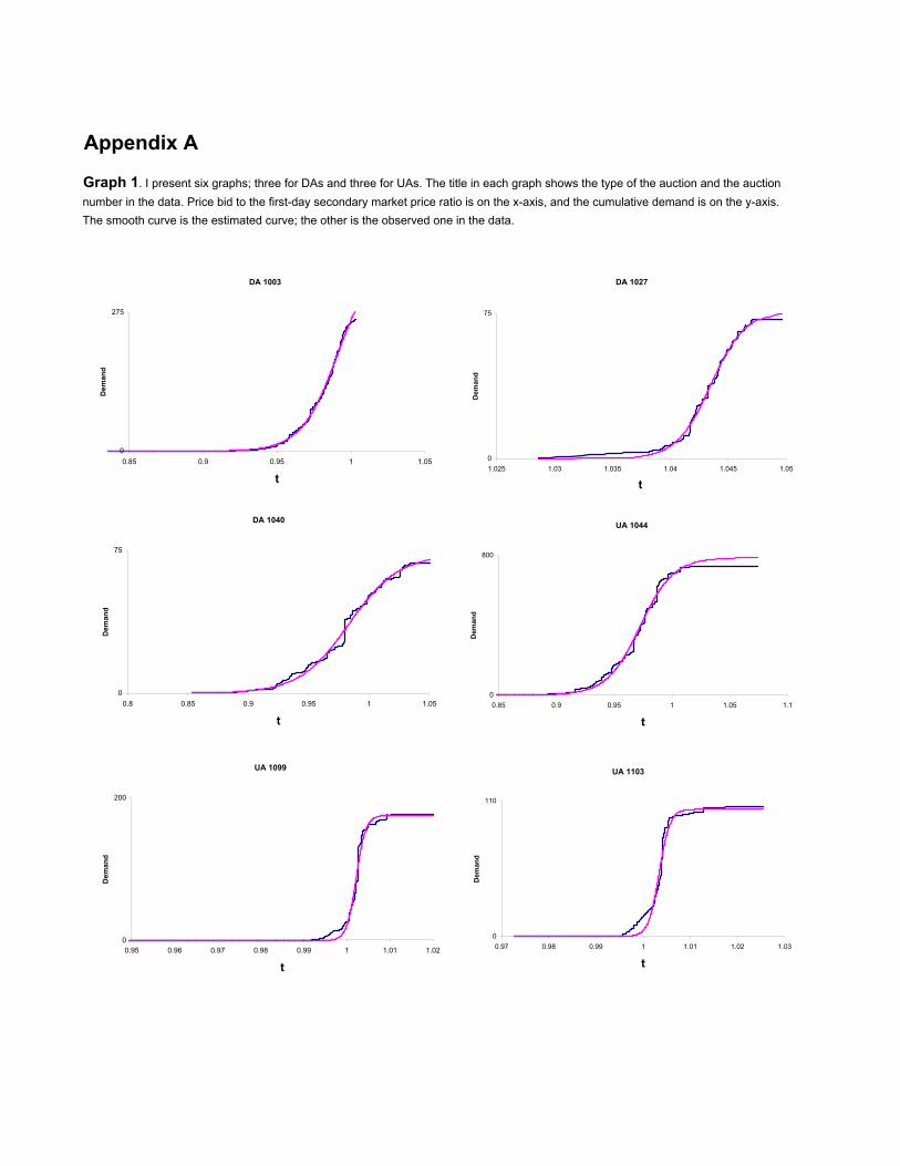
Appendix A presents few examples of aggregate quantity demand curves

plotted against the ratio of the price bids to the first day of the secondary

market price of the bill. Note that all the graphs are sigmoidal in shape.

A sigmoidal curve can be approximated by the following three-parameter

logistic function

y =α

1 + exp (−λ(p− τ)), (1)

where y is the aggregate quantity demand as a function of price bid p.

α > 0, τ > 0, and λ > 0 are the parameters of the function. However,

instead of using price bids, equation (1) can be written in terms of the

normalized price bids t = p/ps, where ps is the first-day secondary market

price of the bill. Hence, I use the following form of the logistic function:

y =α

1 + exp (−λ(t− τ)). (2)

I give the observed cumulative aggregate demand curve and the curve es-

timated by equation (2) in Appendix A. I provide three randomly chosen

graphs for discriminatory auctions (DAs) and uniform auctions (UAs) as a

sample. The number of bids greater than the first-day secondary market

price is higher in UAs. The reason is that bidders pay the minimum ac-

cepted bid instead of their individual bids, and hence the marginal cost of

submitting a high bid is lower in UAs than in DAs. This behavior shows up

as in the graphs on UAs a shift in the curve to the right.

The interpretation of the logistic growth function of the Treasury auc-

tions setup is the following:

6

– At level α, the market demand is satisfied to the fullest: there is no

market demand beyond α. On the graph, it is the height of the S-shape

curve. Mathematically speaking, y → α as t → ∞. Higher demand in theauction means a higher α.

– τ doesn’t change the shape of the curve but determines the inflection

point and the position of the curve. It shows how much price bids deviate

from the first-day secondary market price of the bill. When t = τ , y = α/2,

i.e. the inflection point of the curve is at the halfway point of the market

satisfaction level.

– 1/λ is the measure of the dispersion of the normalized price bids, hence

of the price bids themselves. Higher uncertainty leads to more dispersion,

meaning a lower λ.

The parameter vector of the auction i is denoted as Θi = (αi, τ i,λi)0.

Let tij be the jth observation of the normalized price bid in auction i. I

then estimate the parameters of the logistic function through the following

specification:

yij = f(tij ,Θi) + εij , (3)

where f(tij ,Θi) is defined by equation (2), and εij is a random error.

Equation (3) is estimated by using nonlinear least squares. In order to

show that the logistic function is a good representation not only visually

but also statistically, I regenerate the stop-out and the quantity-weighted

average prices for comparison with the observed values. The stop-out rate,

tsi, is the price at which f(tij ,Θi) = yi, where yi represents the supply in

the auction i, i.e.

tsi = τ i − 1

λilog

µαi − yiyi

¶. (4)

The quantity-weighted average rate twi is calculated by

twi =1

yi

Z tmi

tsi

ti∂yi∂ti(ti)dti, (5)

7

where tmi is the maximum tij .

I compare the estimated stop-out and quantity-weighted price bids with

the observed values to show the goodness-of-fit. The next section describes

the estimation procedure of the parameters from the economic variables.

2.2 Estimating the economic determinants of the estimated

logistic function parameters

In this section, I describe the methodology of estimating the parameter vec-

tor, Θi = (αi, τ i,λi)0, using various economic variables. BL (1999) and BBL

(1999) treat the fluctuations in the market demand function from one auc-

tion to another as random events. However, PW (2004) argue that those

fluctuations, rather than being random events, depend on the economic sit-

uation at the time of the auction. In this paper, fluctuations are also inter-

preted as functions of economic variables. In other words, the fluctuations

are determined by the economic conditions. Using variables representative

of the economic environment at the time of the auction, I estimate the pa-

rameter vector for the logistic function.

In this regard, I estimate parameters using Zellner’s Seemingly Unre-

lated Regression (SUR) model, which controls for the economic variables.

Causality relationships between variables justify the use of SUR. Signifi-

cance levels are computed using the bootstrap method, which also controls

for the small sample bias. This analysis is done separately for DAs and UAs.

Finally, I derive an estimation equation for each parameter of the logistic

function under DAs as well as under UAs. The next section depicts how the

simulations are done to calculate the revenues under both auction methods

by using the parameter estimation equations given in this section.

8

2.3 Simulation method

Using parameter estimation equations for both auction types, this section

describes the method used to compare the two types in terms of their revenue

extraction ability. I consider the equations for each parameter for one type

of auction and use the data for the other type of auction to simulate the

stop-out price. In other words, I take the equations for the parameters that

are estimated for the UAs and calculate the stop-out price using the DAs’

economic conditions. This simulates the UAs under the same economic

situation that existed for the DAs. I also take the equations for DAs and

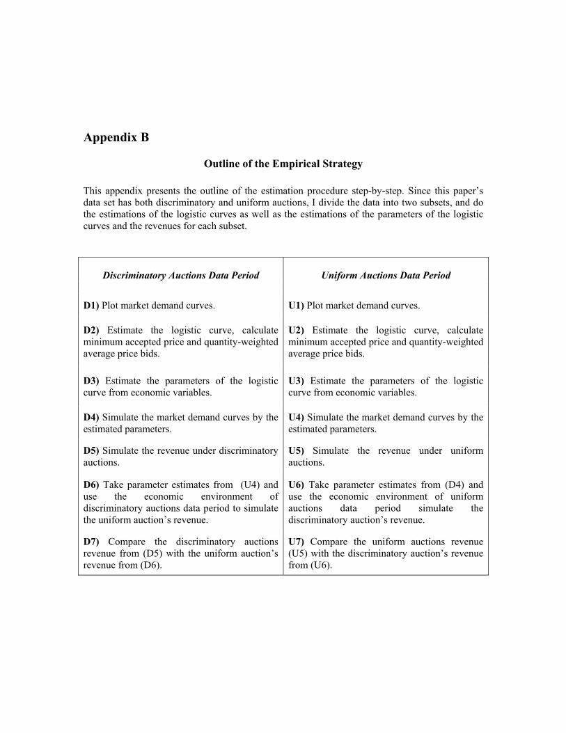
simulate the stop-out price using the UAs’ data. Appendix B gives an outline

of the estimation procedure step-by-step.

Graph 2. This figure shows the graphical representation of revenue calculation under discriminatory and uniform auctions using the market demand curves.

0

20

40

60

80

100

120

0 0.5 1 1.5 2

t

D e m a n d

Graph 2 shows how the revenues are calculated under DAs and UAs.

There are two hypothetical market demand curves, the higher is for uniform

and the lower is for discriminatory auctions. In this example, supply is

assumed to be the same for both auction types, to be consistent with the

9

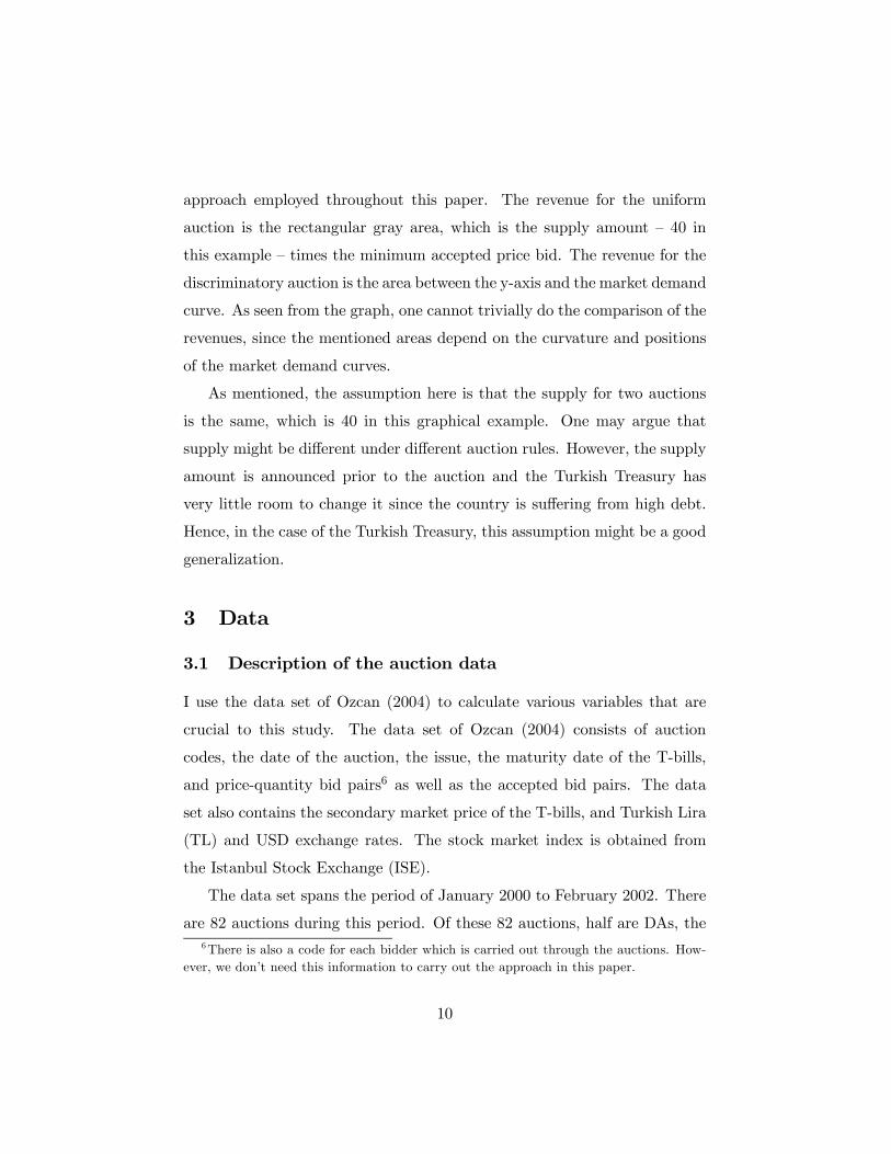
approach employed throughout this paper. The revenue for the uniform

auction is the rectangular gray area, which is the supply amount — 40 in

this example — times the minimum accepted price bid. The revenue for the

discriminatory auction is the area between the y-axis and the market demand

curve. As seen from the graph, one cannot trivially do the comparison of the

revenues, since the mentioned areas depend on the curvature and positions

of the market demand curves.

As mentioned, the assumption here is that the supply for two auctions

is the same, which is 40 in this graphical example. One may argue that

supply might be different under different auction rules. However, the supply

amount is announced prior to the auction and the Turkish Treasury has

very little room to change it since the country is suffering from high debt.

Hence, in the case of the Turkish Treasury, this assumption might be a good

generalization.

3 Data

3.1 Description of the auction data

I use the data set of Ozcan (2004) to calculate various variables that are

crucial to this study. The data set of Ozcan (2004) consists of auction

codes, the date of the auction, the issue, the maturity date of the T-bills,

and price-quantity bid pairs6 as well as the accepted bid pairs. The data

set also contains the secondary market price of the T-bills, and Turkish Lira

(TL) and USD exchange rates. The stock market index is obtained from

the Istanbul Stock Exchange (ISE).

The data set spans the period of January 2000 to February 2002. There

are 82 auctions during this period. Of these 82 auctions, half are DAs, the6There is also a code for each bidder which is carried out through the auctions. How-

ever, we don’t need this information to carry out the approach in this paper.

10

other half are UAs. Bidders submit price-quantity pairs for pure discount

Treasury bills with a face value of TL100,000. Bills do not bear any coupons.

As stated earlier, the Treasury changed the auction format in February 2001

from discriminatory to uniform pricing. The number of price bids for each

auction ranges from 42 to 473 for the DAs, and 92 to 477 for the UAs.

Table 1 shows the maturity structure of the auctions dividing the sample

into discriminatory and uniform auctions. As seen from the table, bills don’t

have a regular maturity structure. Unlike some other countries, in Turkey

there is no regular pattern to issuing the bills. Since Turkey had been going

through a series of economic and financial crises and suffering high domestic

debt with short maturity, it seems that the Treasury conducts auctions just

before high debt payback. Table 1 also shows the total demand and supply

and the averages for each of the maturities. The cover ratio, the satisfied

portion of the demand, is given in percentages. Both demand and supply

are lower for the uniform auction period. The cover ratio is higher in the

uniform auction period. There are also more bills with short maturities in

the uniform auctions.

I calculate the cumulative aggregate quantity bids from the individual

price-quantity bids for each price bid. Unlike PW (2004) who use interest

rate bids, I use price bids in the analysis. As do BL (1999), I normalize the

price bids by the first-day secondary market price of that bill. I calculate

auction-specific variables. The variables include the maturity of the bill

auctioned, total supply, the first-day secondary market price of the auctioned

bill, whether the auction is undertaken at the end of the month, whether

there is another auction at the same day, and whether the bill is auctioned

for the first time. In addition, the trading volume of the stock market and

the variance of the overnight interest rates prior to the auction are included

in the variables in order to fully simulate the economic conditions at the

11

12

Table 1. Summary statistics of the data. The top panel reports results for discriminatory auctions. The bottom panel reports results for uniform auctions. Maturity is in months, and number of auctions shows the corresponding number of auctions. Aggregate demand and aggregate supply are in columns three and five respectively. The averages are given in columns four and six. All the monetary values are given in million $US by using the exchange rate at the time of the auction. The cover ratio is calculated as the percentage of the satisfied demand in the last column.

Discriminatory

Auctions

Maturity Number of Auctions

Aggregate Demand

Average Demand

Aggregate Supply

Average Supply

Cover Ratio (%)

1 1 257.68 257.68 232.73 232.73 90.32

3 10 1691.88 169.19 944.52 94.45 55.83

6 1 352.46 352.46 222.25 222.25 63.06

12 3 793.49 264.50 339.03 113.01 42.73

13 3 1214.38 404.79 559.33 186.44 46.06

14 6 1480.70 246.78 909.99 151.66 61.46

16 5 2270.71 454.14 997.05 199.41 43.91

18 3 665.45 221.82 270.59 90.20 40.66

24 9 1604.18 178.24 583.14 64.79 36.35

TOTAL 41 10330.92 251.97 5058.63 123.38 48.97

Uniform Auctions

Maturity Number of Auctions

Aggregate Demand

Average Demand

Aggregate Supply

Average Supply

Cover Ratio (%)

3 11 1717.99 156.18 892.62 81.15 51.96

4 4 527.30 131.82 424.20 106.05 80.45

5 5 571.71 114.34 374.66 74.93 65.53

6 6 726.10 121.02 505.78 84.30 69.66

7 3 331.32 110.44 283.94 94.65 85.70

8 4 465.79 116.45 319.09 79.77 68.51

10 4 385.83 96.46 260.90 65.22 67.62

12 1 190.02 190.02 91.49 91.49 48.15

13 3 213.75 71.25 168.71 56.24 78.93

24 1 179.76 179.76 89.41 89.41 49.74

TOTAL 42 5309.56 126.42 3410.81 81.21 64.24

time of the auction. I calculate the minimum accepted price bid (the stop-

out price) and the quantity-weighted average of the accepted price bids in

order to compare these with the estimation results.

There are two arguments by PW (2004) against using the individual bid

functions. First, there are few observations with which to estimate individual

bid functions. Second, the Treasury uses the market bid function, not the

individual bid functions. Hortacsu and Ozcan (2004) also use the data set

prepared by Ozcan (2004) to show that individual bid functions can be

approximated by linear functions. Hence the first argument is not valid for

this paper’s data set. However, given BL’s (1999) argument — central banks

in almost all countries record the data by aggregating rather than keeping

the individual bids — and the fact that the given Treasury uses the market

bid function, we may have sufficient motivation to study the aggregate bid

functions.

There are on average 192 price bids in the DA part of the data, and 247

in the UA part of the data. The average number of winning price bids is

88 in DAs and 136 in UAs. The average number of bidders in DAs is 56,

whereas in UAs it is 80. This finding shows that the Treasury achieved an

increase in participation by switching to uniform auctions. This is consistent

with the argument that UAs increase participation since in DAs it is costlier

to bid, both because bid decision requires more specialization and because

the winners’ curse is high (if one wins, one pays more than the stop-out

price). Indeed, the same observation is also valid for the average number of

the winners: 37 in the DAs and 67 in the UAs.

3.2 Other economic data

Before I calculate the aggregate quantity demand and plot it against the

ratio of the price bids to the first-day price of the bill on the secondary

13

market, I drop upper and lower 0.5% of the observations in each auction

to eliminate the outliers such as bidding mistakes and unrealistic bid pairs.

This eliminates 100 observations out of 18,330.

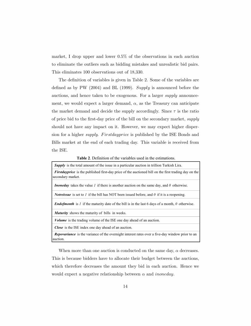
The definition of variables is given in Table 2. Some of the variables are

defined as by PW (2004) and BL (1999). Supply is announced before the

auctions, and hence taken to be exogenous. For a larger supply announce-

ment, we would expect a larger demand, α, as the Treasury can anticipate

the market demand and decide the supply accordingly. Since τ is the ratio

of price bid to the first-day price of the bill on the secondary market, supply

should not have any impact on it. However, we may expect higher disper-

sion for a higher supply. Firstdayprice is published by the ISE Bonds and

Bills market at the end of each trading day. This variable is received from

the ISE.

Table 2. Definition of the variables used in the estimations.

Supply is the total amount of the issue in a particular auction in trillion Turkish Lira.

Firstdayprice is the published first-day price of the auctioned bill on the first trading day on the secondary market.

Inoneday takes the value 1 if there is another auction on the same day, and 0 otherwise.

Notreissue is set to 1 if the bill has NOT been issued before, and 0 if it is a reopening.

Endofmonth is 1 if the maturity date of the bill is in the last 6 days of a month, 0 otherwise.

Maturity shows the maturity of bills in weeks.

Volume is the trading volume of the ISE one day ahead of an auction.

Close is the ISE index one day ahead of an auction.

Repovariance is the variance of the overnight interest rates over a five-day window prior to an auction.

When more than one auction is conducted on the same day, α decreases.

This is because bidders have to allocate their budget between the auctions,

which therefore decreases the amount they bid in each auction. Hence we

would expect a negative relationship between α and inoneday.

14

Since the first-day secondary market price is more uncertain for a bill is-

sued for the first time than for a bill issued before, notreissue has a negative

impact on τ .We may also argue that as the reissued bill is readily available

on the secondary market, bidders may choose to buy it on the secondary

market instead of participating in the auction. Hence α goes down for the

reissues. Park and Reinganum (1986) show that bills with a maturity date

in the last week of a month have lower yields. In addition, Simon (1994b)

finds that bills maturing at month-ends tend to have lower yields than those

maturing earlier in the month.

A negative relation between maturity and the parameter τ is expected.

This is because the variance of the bidders’ belief of the price of a security

with longer maturity is higher than it is for one with shorter maturity.

Hence, the difference between the first-day price of the security and the price

bids at an auction increases, and the price bids decrease as well, leading to

a negative relation.

Stocks are considered as an alternative investment venue to bills. If the

volume of the stock market is high, we would expect less demand for the

bills. As the ISE index one day ahead of an auction, close, goes up, we may

expect less demand in the auction. Bidders may choose to invest instead

in the stock market, which will lower α. The repovariance variable is used

as an indicator of the financial and economic situation at the time of the

auction.

4 Estimating the Logistic Function Parameters for

Each Auction

I first estimate the parameters of equation (2) following the procedure de-

scribed in section 2.1. The results indicate that the logistic function ap-

15

proach describes the aggregate market demand very well.

The graphs of aggregate market demand versus the price ratio and the

estimated logistic function suggest that the logistic functional approach pro-

vide a good description of the data. However, we need to show that the

correlation between the estimated curve and the data points is high in order

to validate the visual judgment. To this end, I calculate the stop-out and

quantity-weighted winning price bids from both the data and the estimated

curve just as described in equations (4) and (5). The results are given in

Table 3.

Table 3. Stop-out price is calculated from the estimated curve as the minimum accted price bid. Min accepted

price is the observed minimum accepted price bid in the data. Fourth and fifth columns show the quantity-weighted

prices calculated from the estimated curve and the data, respectively.

Stop-out Price

Min Accepted Price

Observed Q-Weighted Price

Estimated Q-Weighted Price

Discriminatory Auctionsmean 82,256 82,322 82,662 82,718Stdev 13,983 13,755 13,720 13,789

Uniform Auctionsmean 76,546 76,252 76,818 76,846Stdev 9,842 9,892 9,697 9,718

As seen from Table 3, the estimated and observed minimum and quantity-

weighted prices are close to each other. In fact, the correlation coefficients

between the estimated and observed prices are 0.997 and 0.999 for the min-

imum and weighted prices under the UA rule, respectively. If we perform

hypothesis testing for the difference of the means of minimum and weighted

prices, we find that the hypothesis that the means are equal cannot be re-

jected. Therefore, I conclude that the logistic function approach describes

the aggregate market demand very well.

16

The next section estimates the parameters of the logistic function from

economic variables using Zellner’s SUR regressions.

5 Estimating the Economic Determinants of the

Logistic Function Parameters

I estimate the parameters of equation (3) from a set of economic variables in

order to explain the parameters’ fluctuations from one auction to another.

The economic variables used in the Zellner’s SUR model are the maturity in

weeks, total supply in the auction, first-day price of the auctioned bill on the

secondary market, the stock market index and volume, the five-day variance

of the overnight interest rates prior to the auction date, and two dummy

variables. One dummy variable takes the value of 1 if there is another

auction on the same day, and 0 otherwise. The other takes the value of 1

if the bill is a reissue, and 0 otherwise. I also include a dummy variable

showing that the maturity date of the security is in the last 6 days of the

month.

I use bootstrap regressions to correct for the small sample bias. This is

done for DAs and UAs separately. For the DAs, I use the same regression

equation for all three parameters. However, we get a better fit by changing

the regression equations for UAs. I add the five-day overnight interest rate

variance prior to an auction, and replace the stock market volume with

the stock market index in the regression equations of α and λ. Zellner’s

SUR regressions reveal that the parameters of the logistic function can be

estimated using the economic variables, and that the economic variables can

explain the fluctuations in the parameters from one auction to another. The

results are shown in Table 4.

17

18

Table 4. The results of Zellner's SUR model for estimating the parameters of the logistic function from economic variables. The left-hand side gives the results for the discriminatory auctions; the right-hand side is for the uniform auctions. *, **, and *** show significance at the 10%, 5%, and 1% level, respectively.

Discriminatory Auctions Uniform Auctions

Coefficient Standard Error Coefficient Standard

Error

Alpha Alpha

maturity (in weeks) 0.6596 ** 0.4018 0.7378 * 0.6023 maturity (in weeks)

inoneday -30.8344 29.2073 53.5474 * 26.9011 inoneday

supply 1.4356 *** 0.2201 1.1460 *** 0.1435 supply

firstdayprice -0.0012 0.0008 0.0013 * 0.0010 firstdayprice

notreissue 26.4436 25.2112 23.5837 20.3843 notreissue

voltrillion 0.0245 0.0561 -0.0152 *** 0.0057 close

endofmonth -19.8911 54.2471 13.4314 22.6497 endofmonth

constant 128.2182 75.1781 79974.8300 23863.79 repovariance

33.0355 90.5279 constant

Lambda Lambda

maturity(in weeks) -3.3148 ** 1.2984 -6.8593 *** 2.2961 maturity(in weeks)

inoneday 5.8864 94.3900 -174.1590 * 102.0565 inoneday

supply -0.6479 0.7115 -0.6050 0.5445 supply

firstdayprice 0.0076 *** 0.0027 0.0102 0.0038 firstdayprice

notreissue 75.5355 81.4759 -200.4339 ** 77.3294 notreissue

voltrillion -0.0556 0.1812 0.0566 ** 0.0225 close

endofmonth -55.5670 175.3118 -84.9092 85.9285 endofmonth

constant 19.2797 242.9552 151426.6000 91019.70 repovariance

-615.2171 346.8189 constant

Tau Tau

maturity(in weeks) -0.0000099 0.0001154 -0.0001063 0.0000966 maturity(in weeks)

inoneday -0.0056025 0.0083919 -0.0009264 0.0046349 inoneday

supply 0.0000418 0.0000633 -0.0000011 0.0000242 supply

firstdayprice 0.0000005 ** 0.0000002 0.0000001 0.0000002 firstdayprice

notreissue -0.0047261 0.0072437 -0.0031210 0.0034705 notreissue

voltrillion -0.0000127 0.0000161 0.0000154 ** 0.0000078 voltrillion

endofmonth -0.0044249 0.0155864 -0.0066317 0.0037770 endofmonth

constant 0.9648085 **** 0.0216003 -1.6064300 3.8033740 repovariance

0.9943357 **** 0.0141440 constant

As expected, the supply amount is the most important variable affecting

market saturation level, α, in both DAs and UAs. Similar to the results of

PW (2004), BL (1999) and BBL (1999), it has a positive coefficient, i.e. as

supply increases the market saturation level increases. Maturity also plays

a role in determining the value of α. It has a positive coefficient. In UAs,

the stock market index affects α inversely. This can be explained as follows:

as the ISE index goes up, investors lean more toward buying stocks than

participating in auctions. This variable is significant only in the case of

UAs, supporting the argument that UAs attract more investors and that

generally these investors have smaller portfolios. As some investors move

toward buying stocks, their budget is depleted at a low level of α.

Under DAs, maturity affects the price bid dispersion negatively. This

negative relation indicates that as maturity increases, the price bids become

more dispersed. Either every bidder increases the difference between her

maximum and minimum price bids, or, even if they don’t change the differ-

ence between their maximum and minimum price bids, the variance across

bidders increases, and hence the overall dispersion on the aggregate market

demand curve increases. The first-day price of a bill on the secondary mar-

ket, however, has a positive effect on the price bid dispersion (and a negative

effect on λ as dispersion is 1/λ), i.e. as the first-day secondary market price

of a bill increases, price dispersion in the auction decreases. One explana-

tion of this might be that because of the bad performance of the Turkish

economy during the data period, a higher first-day price on the secondary

market might signal a better economic outlook. Hence, bidders can make

better forecasts, and this leads to lower levels of price bid dispersion in the

auction.

For UAs, maturity has the same effect as it does for DAs. There is a neg-

ative relation between λ and the auctions done in the same day (inoneday)

19

and the reissued auctions. It seems that having more than one auction on

the same day increases the price bid spread. If a bill is issued for the first

time (notreissue = 1), the uncertainty about its price is high compared to

the price of a bill that has been issued before and traded in the secondary

market. Hence the sign of the coefficient follows.

Under DAs, people care about the first-day price of the security, i.e it

has a positive significant coefficient. As the first-day price rises, τ rises, and

hence the logistic curve shifts to the right. One interpretation of this might

be that in DAs bidders have to pay their bids, and hence they watch the

secondary market price more closely in order to avoid the winner’s curse.

However, in UAs, instead of the first-day price, the volume of the stock

market has a positive and significant coefficient.

Using estimation equations, I calculate the parameters. Then equation

(2) gives the aggregate market demand function. I calculate the stop-out and

weighted average prices using these equations. The correlation coefficient of

the in-sample forecasts of the stop-out price and the observed minimum

price is 0.997; the estimated weighted price and the observed weighted price

is 0.999 for the DAs. The corresponding values for the UAs are 0.996 and

0.999, respectively.

5.1 Out-of-sample forecast

I forecast the stop-out and weighted prices of a few auctions using a part

of the data set. In order to make the out-of-sample forecast, I first exclude

5 auctions from the DAs’ data. Following the above lines,7 I estimate the

parameters. Then, using these parameter values, I calculate the stop-out

and weighted prices. The corresponding correlation coefficients are 0.9977 I do all the bootstrap and Zellner’s SUR regressions with a smaller number of auctions.

I then estimate the parameters, α,λ, and τ .

20

for the observed minimum and the estimated stop-out price; and 0.999 for

the observed and estimated weighted prices for the DAs.

The same procedure is also undertaken for the UAs. The correlation

coefficients are 0.757 and 0.983 for the estimated and observed minimum

prices and the estimated and observed weighted prices.

6 Simulations

In this section, I implement the results from Section 5. The first part of

the analysis is as follows: using the parameter estimates and using the DAs’

part of the data, I calculate the stop-out and the weighted average prices.

Table 5. In Panel A, there are minimum and q-weighted prices both observed in the DA and estimated for UA.

In Panel B, we have the observed variables for the UA prices, and estimated DA prices.

Panel A Panel B

Discriminatory Part Uniform Part

Variable Mean Std. Dev. Mean Std. Dev. Variable

Minimum DA price 80,846 15,195 75,835 10,226 Stop-out DA price

Weighted observed DA price

81,234 15,125 76,629 9,763 Weighted estimated DA price

Stop-out UA price 80,656 15,215 76,232 9,769 Minimum UA price

Weighted estimated UA price

81,175 15,092 76,784 9,578 Weighted observed UA price

Panel A of Table 5 summarizes the estimated and observed prices for the

DAs’ part of the data. In Panel A, the mean of the minimum and weighted

average prices observed in the data for DAs are 80,846 and 81,234, which are

shown in the first and second rows, respectively. The mean of the calculated

minimum price and the weighted average prices, estimated using the uniform

21

pricing rule, are 80,656 and 81,175, respectively. The details can be seen in

the third and fourth rows of Panel A. The mean of the observed minimum

prices for DAs, 80,846, is greater than the mean of the estimated stop-out

rate, 80,656, if we had used UAs. The same relation is also true for the

mean of the weighted average prices. This result contradicts the claim that

in DAs bidders shade their bids more than they do in UAs. This empirical

finding is important because, to the best of our knowledge, this is the first

comparison of the two auction types under the same economic conditions.

The only assumption is that the supply for both types of auctions is the

observed amount, as mentioned in section 2.3.

The second part of the analysis involves reverse calculations. Reverse

calculations may give us more insight into the comparison of both auction

types. I consider the equations, which are used to acquire parameter esti-

mates for DAs, and use them to estimate parameters with the economic

variables during the UA period. I calculate the estimated stop-out and the

weighted average prices under DAs instead of UAs. The results are in Ta-

ble 5, Panel B. The mean of the estimated weighted average prices under

DAs, which is 76,629, is less than the mean of the observed weighted aver-

age prices under UAs, 76,784. This result contradicts the first finding. The

mean of the estimated stop-out prices under DAs is 75,835, which is less

than the mean of the observed UAs’ minimum prices, 76,232. Hence, this

finding supports the claim that the minimum price is less under DAs than

it is under UAs.

I also calculate the revenue of the Treasury under the two auction types

by using the calculated minimum prices and the aggregate market demand

curves. Table 6 shows the simulated revenues under different auction types.

22

Table 6. The estimated revenues of the different auction types under the same economic conditions.

Revenue under Disc. Auction

Revenue under Uniform Auction

Disc. Auc. Data 93.680 82.580

Unif. Auc. Data 58.039 61.271

During the actual discriminatory auctions period, the revenue estima-

tions reveal that DAs generate more revenue than UAs. The revenue under

discriminatory auctions is 93 million $US on the average, whereas it would

have been 82 million $US if the uniform auction type were employed dur-

ing that period. However, during the actual uniform auctions period, the

average revenue is 61 million $US, which is a little greater than the average

revenue, 58 million $US, if discriminatory auctions had been employed dur-

ing that period. This result may be due to the fact that in the estimations

the supply is not changed to reflect a change in auction type. The Treasury

might choose to change the supply, or the frequency of auctions depending

on the type of the auction employed; these questions are left for future re-

search. Although the discriminatory versus uniform auction puzzle remains,

it can be concluded that discriminatory auctions raise more revenue for the

Treasury than uniform auctions. This is because the discriminatory auc-

tions data so strongly favor discriminatory auctions, whereas the uniform

auctions data favor uniform auctions by a smaller margin.8.

8One may argue that revenue is not the only concern. There may be other concerns suchas maintaining the liquidity of the secondary market, or protecting small investors, etc.However, in Turkish auctions, we may assume the Threasury cares more about revenue,as the country suffers high domestic and foreign debt.

23

7 Conclusion

This paper employs an empirical method proposed by BL (1999) to analyze

Treasury auctions. Instead of considering individual bid functions and bid-

ders, I consider the aggregate market bid functions. Like BL (1999), BBL

(1999), and PW (2004), I show that the logistic growth curve represents the

market bid function very well. Unlike BL (1999) and BBL (1999), which

treat the fluctuations from one auction to another as random, I consider, like

PW (2004), the fluctuations to be a function of economic variables. Hence,

I estimate the parameters the logistic function by using the economic and

auction-specific variables.

First, I estimate the parameters of the logistic function. I then show that

in-sample and out-of-sample forecasts fit the data very well. Therefore, I

conclude the aggregate market bid function can be approximated fairly well

using the logistic function.

The comparison between discriminatory and uniform auctions is an on-

going debate that requires much research. However, this paper diverges from

the literature in that it compares the auction types while economic condi-

tions constant. This paper is the first study in the literature that empirically

compares the amount of revenue extracted for the Treasury by simulating

the same economic environment under both auction types. Having both

types of auction in the data set enables us to perform such a comparison.

Elimination of any change in the economic conditions yields a much better

comparison. The revenue comparison results are contradictory; however,

as the revenues of both types are very close during the uniform auctions

period, whereas the discriminatory auctions produce much higher revenue

than would the uniform auctions during the discriminatory auctions period,

I conclude that discriminatory pricing is better for the Treasury. However,

this conclusion should be supported in future studies by taking into account

24

the trade-off between frequency and volume of auctions, and the maturity

of the security, and the possibility of changing supply in different auction

types.

25

References

[1] Back, K., and Zender, J. F., 1993. Auctions of Divisible Goods: on the

Rationale for the Treasury Experiment. Review of Financial Studies 6(4),

733-764.

[2] Berg, S.A., Boukai, B., and Landsberger, M., 1999. Bid Functions for Trea-

sury Securities; Across Countries Comparison. Mimeo.

[3] Binmore, K., and Swierzbinski, J., 2000. Treasury Auctions: Uniform or

Discriminatory. Review of Economic Design 5, 387-410.

[4] Boukai, B., and Landsberger, M., 1999. Market Bid Functions for Treasury

Securities as Logistic Curves. Mimeo.

[5] Heller, D., and Lengwiler, Y., 1998. The Auctions of Swiss Government

Bonds: Should the Treasury Price Discriminate or Not? Mimeo, Swiss

National Bank and Board of Governors of the Federal Reserve System.

[6] Hortacsu, A., 2003. Mechanism Choice and Strategic Bidding in Divisible

Good Auctions: An Empirical Analysis of the Turkish Treasury Auction

Market. Mimeo.

[7] Nautz D., 1995. Optimal Bidding in Multi-Unit Auctions with Many Bid-

ders. Economics Letters 48, 301-306.

[8] Ozcan, R., 2004. Are Bidders Buddies in Treasury Auctions? The Turkish

Case. Mimeo, Boston College.

[9] Park, S.Y., and Reinganum, M.R., 1986. The Puzzling Price Behavior of

Treasury Bills That Mature at the Turn of Calendar Months. Journal of

Financial Economics 16, 267-283.

26

[10] Preget, R., and Waelbroeck, P., 2005. Treasury Bill Auction Procedures:

Empirical Perspectives from French Market Bid Functions. Journal of In-

ternational Money and Finance, 24, 1054-1072.

[11] Simon, D. P., 1994a. The Treasury’s Experiment with Single-Price Auctions

in the mid-1970s: Winner’s or Taxpayer’s Curse? The Review of Economics

and Statistics 76 (4), 754-760.

[12] Simon, D. P., 1994b. Further Evidence on Segmentation in the Treasury

Bill Market. Journal of Banking and Finance 18, 139-151.

[13] Umlauf, S. R., 1993. An Empirical Study of the Mexican Treasury Bill

Auction. Journal of Financial Economics 33, 313-340.

[14] Wang, J. J. D., and Zender, J. F., 2002. Auctioning Divisible Goods. Eco-

nomic Theory 19, 673-705.

[15] Wilson, R., 1979. Auctions of Shares. Quarterly Journal of Economics, 93

(4), 675-689.

27

Appendix A

Graph 1. I present six graphs; three for DAs and three for UAs. The title in each graph shows the type of the auction and the auction number in the data. Price bid to the first-day secondary market price ratio is on the x-axis, and the cumulative demand is on the y-axis. The smooth curve is the estimated curve; the other is the observed one in the data.

DA 1003

0

275

0.85 0.9 0.95 1 1.05

t

Dem

and

DA 1027

0

75

1.025 1.03 1.035 1.04 1.045 1.05

tD

eman

d

DA 1040

0

75

0.8 0.85 0.9 0.95 1 1.05

t

Dem

and

UA 1044

0

800

0.85 0.9 0.95 1 1.05 1.1

t

Dem

and

UA 1099

0

200

0.95 0.96 0.97 0.98 0.99 1 1.01 1.02

t

Dem

and

UA 1103

0

110

0.97 0.98 0.99 1 1.01 1.02 1.03

t

Dem

and

Appendix B

Outline of the Empirical Strategy This appendix presents the outline of the estimation procedure step-by-step. Since this paper’s data set has both discriminatory and uniform auctions, I divide the data into two subsets, and do the estimations of the logistic curves as well as the estimations of the parameters of the logistic curves and the revenues for each subset.

Discriminatory Auctions Data Period

Uniform Auctions Data Period

D1) Plot market demand curves. U1) Plot market demand curves.

D2) Estimate the logistic curve, calculate minimum accepted price and quantity-weighted average price bids.

U2) Estimate the logistic curve, calculate minimum accepted price and quantity-weighted average price bids.

D3) Estimate the parameters of the logistic curve from economic variables.

U3) Estimate the parameters of the logistic curve from economic variables.

D4) Simulate the market demand curves by the estimated parameters.

U4) Simulate the market demand curves by the estimated parameters.

D5) Simulate the revenue under discriminatory auctions.

U5) Simulate the revenue under uniform auctions.

D6) Take parameter estimates from (U4) and use the economic environment of discriminatory auctions data period to simulate the uniform auction’s revenue.

U6) Take parameter estimates from (D4) and use the economic environment of uniform auctions data period simulate the discriminatory auction’s revenue.

D7) Compare the discriminatory auctions revenue from (D5) with the uniform auction’s revenue from (D6).

U7) Compare the uniform auctions revenue (U5) with the discriminatory auction’s revenue from (U6).