diffraction â€“ plane-wave spectrum

$: Diffraction â€“ Plane-Wave Spectrum$
18.16. Problems 843

18.9 Consider a reflector antenna fed by a horn, as shownon the right. A closed surface S = Sr + Sa is suchthat the portion Sr caps the reflector and the portionSa is an aperture in front of the reflector. The feedlies outside the closed surface, so that the volume Venclosed by S is free of current sources.

Applying the Kottler version of the extinction theorem of Sec. 18.10 on the volume V, showthat for points r outsideV, the field radiated by the induced surface currents on the reflectorSr is equal to the field radiated by the aperture fields on Sa, that is,

E rad(r) = 1

jωε

∫Sr

[k2G J s +

(J s ·∇∇∇′

)∇∇∇′G]dS′= 1

jωε

∫Sa

[k2G(n×H )+((n×H )·∇∇∇′)∇∇∇′G+ jωε(n× E )×∇∇∇′G]dS′

where the induced surface currents on the reflector are J s = nr ×H and Jms = −nr ×E, andon the perfectly conducting reflector surface, we must have Jms = 0.

This result establishes the equivalence of the so-called aperture-field and current-distributionmethods for reflector antennas [1686]. See also Sec. 21.9.

18.10 Consider an x-polarized uniform plane wave incident obliquely on the straight-edge apertureof Fig. 18.14.4, with a wave vector direction k1 = z cosθ1 + y sinθ1. First show that thetangential fields at an aperture point r′ = x′ x+y′ y on the aperture above the straight-edgeare given by:

Ea = xE0e−jky′ sinθ1 , Ha = y

E0

η0cosθ1e−jky

′ sinθ1

Then, using Kottler’s formula (18.12.1), and applying the usual Fresnel approximations inthe integrand, as was done for the point source in Fig. 18.14.4, show that the diffractedwave below the edge is given by Eqs. (18.14.23)–(18.14.25), except that the field at the edgeis Eedge = E0, and the focal lengths are in this case F = l2 and F′ = l2/ cos2 θ2

Finally, show that the asymptotic diffracted field (when l2 → ∞), is given near the forwarddirection θ � 0 by:

E = Eedgee−jkl2√l2

1− j2√πkθ

18.11 Assume that the edge in the previous problem is a perfectly conducting screen. Using thefield-equivalence principle with effective current densities on the aperture above the edgeJ s = 0 and Jms = −2n× Ea, and applying the usual Fresnel approximations, show that thediffracted field calculated by Eq. (18.4.1) is still given by Eqs. (18.14.23)–(18.14.25), exceptthat the factor cosθ1+ cosθ2 is replaced now by 2 cosθ2, and that the asymptotic field andedge-diffraction coefficient are:

E = E0e−jkl2√l2Dedge , Dedge = (1− j)2 cosθ2

4√πk(sinθ1 + sinθ2)

Show that this expression agrees with the exact Sommerfeld solution (18.15.26) at normalincidence and near the forward diffracted direction.

19Diffraction – Plane-Wave Spectrum

This chapter continues the previous one on radiation from apertures. The emphasisis on Rayleigh-Sommerfeld diffraction theory, plane-wave spectrum representation forscalar and vector fields, radiated and reactive power of apertures, integral equationsfor apertures in conducting screens, revisiting the Sommerfeld half-plane problem us-ing Wiener-Hopf factorization techniques, the Bethe-Bouwkamp model of diffraction bysmall holes, and the Babinet principle.

19.1 Rayleigh-Sommerfeld Diffraction Theory

In this section, we recast Kirchhoff’s diffraction formula in a form that uses a Dirich-let Green’s function (i.e., one that vanishes on the boundary surface) and obtain theRayleigh-Sommerfeld diffraction formula. In the next section, we show that this re-formulation is equivalent to the plane-wave spectrum approach to diffraction, and useit to justify the modified forms (18.1.2) and (18.1.3) of the field equivalence principle.In Chap. 20, we use it to obtain the usual Fresnel and Fraunhofer approximations anddiscuss a few applications from Fourier optics.

We will work with the scalar case, but the same method can be used for the vectorcase. With reference to Fig. 19.1.1, we consider a scalar field E(r) that satisfies thesource-free Helmholtz equation, (∇2 + k2)E(r)= 0, over the right half-space z ≥ 0.

We consider a closed surface consisting of the surface S∞ of a sphere of very largeradius centered at the observation point r and bounded on the left by its intersection Swith the xy plane, as shown in the Fig. 19.1.1. Clearly, in the limit of infinite radius, thevolume V bounded by S+S∞ is the right half-space z ≥ 0, and S becomes the entire xyplane. Applying Eq. (18.10.3) to volume V, we have:∫

V

[G(∇′2E + k2E)−E (∇′2G+ k2G)

]dV′ = −

∮S+S∞

[G∂E∂n′

− E ∂G∂n′

]dS′ (19.1.1)

The surface integral over S∞ can be ignored by noting that n is the negative of theradial unit vector and therefore, we have after adding and subtracting the term jkEG:

−∫S∞

[G∂E∂n′

− E ∂G∂n′

]dS′ =

∫S∞

[G(∂E∂r

+ jkE)− E

(∂G∂r

+ jkG)]dS′

19.1. Rayleigh-Sommerfeld Diffraction Theory 845

Fig. 19.1.1 Fields determined from their values on the xy-plane surface.

Assuming Sommerfeld’s outgoing radiation condition:

r(∂E∂r

+ jkE)→ 0 , as r →∞

and noting that G = e−jkr/4πr also satisfies the same condition, it follows that theabove surface integral vanishes in the limit of large radius r. Then, in the notation ofEq. (18.10.4), we obtain the standard Kirchhoff diffraction formula, where the planarsurface S is the entire xy plane,

E(r)uV(r)=∫S

[E∂G∂n′

−G ∂E∂n′

]dS′ (19.1.2)

Thus, if r lies in the right half-space, the left-hand side will be equal to E(r), and if ris in the left half-space, it will vanish. Given a point r = (x, y, z), we define its reflectionrelative to the xy plane by r− = (x, y,−z). The distance between r− and a source pointr′ = (x′, y′, z′) can be written in terms of the distance between the original point r andthe reflected source point r′− = (x′, y′,−z′):

R− = |r− − r′| =√(x− x′)2+(y − y′)2+(z+ z′)2 = |r− r′−|

whereasR = |r− r′| =

√(x− x′)2+(y − y′)2+(z− z′)2

This leads us to define the reflected Green’s function:

G−(r, r′)= e−jkR−4πR−

= G(r− r′−)= G(r− − r′) (19.1.3)

846 19. Diffraction – Plane-Wave Spectrum

and the Dirichlet Green’s function:

Gd(r, r′)= G(r, r′)−G−(r, r′)= e−jkR

4πR− e

−jkR−4πR−

(19.1.4)

For convenience, we may choose the origin to lie on the xy plane. Then, as shownin Fig. 19.1.1, when the source point r′ lies on the xy plane (i.e., z′ = 0), the functionGd(r, r′) will vanish because R = R−. Next, we apply Eq. (19.1.2) at the observationpoint r in the right half-space and at its reflection in the left half-plane, where (19.1.2)vanishes:

E(r) =∫S

[E∂G∂n′

−G ∂E∂n′

]dS′ , at point r

0 =∫S

[E∂G−∂n′

−G− ∂E∂n′]dS′ , at point r−

(19.1.5)

where G− stands for G(r− − r′). But on the xy plane boundary, G− = G so that if wesubtract the two expressions we may eliminate the term ∂E/∂n′, which is the reasonfor using the Dirichlet Green’s function:

E(r)=∫SE(r′)

∂∂n′

(G−G−)dS′ =∫SE(r′)

∂Gd∂n′

dS′

On the xy plane, we have n = z, and therefore

∂G∂n′

= ∂G∂z′

∣∣∣∣z′=0

and∂G−∂n′

= ∂G−∂z′

∣∣∣∣z′=0

= − ∂G∂z′

∣∣∣∣z′=0

Then, the two derivative terms double resulting in the Rayleigh-Sommerfeld (type-1)diffraction integral [1286,1287]:

E(r)= 2

∫SE(r′)

∂G∂z′

dS′ = −2∂∂z

∫SE(r′)GdS′ (Rayleigh-Sommerfeld) (19.1.6)

The indicated derivative of G can be expressed as follows:

−∂G∂z

∣∣∣∣z′=0

= ∂G∂z′

∣∣∣∣z′=0

= zR

(jk+ 1

R

)e−jkR

4πR(19.1.7)

To clarify the notation, we may write Eq. (19.1.6) in the more explicit form using (19.1.7),

E(x, y, z)= 2

∫∫∞−∞

zR

(jk+ 1

R

)e−jkR

4πRE(x′, y′,0)dx′dy′ (19.1.8)

where R =√(x− x′)2+(y − y′)2+z2. For distances R λ, or equivalently, k 1/R,

one obtains the approximation:

∂G∂z′

∣∣∣∣z′=0

= jk zRe−jkR

4πR, for R λ (19.1.9)

This approximation will be used in Sec. 20.1 to obtain the standard Fresnel diffractionrepresentation. The quantity z/R is an “obliquity” factor and is usually omitted forparaxial observation points that are near the z axis.

19.1. Rayleigh-Sommerfeld Diffraction Theory 847

Equation (19.1.8) expresses the field at any point in the right half-space (z ≥ 0) interms of its values on the xy plane. For z < 0, the sign in the right-hand side of (19.1.6)must be reversed. This follows by using a left hemisphere enclosing the space z < 0, inthe limit of large radius, and noting that now n = −z, and assuming that E(x, y, z) stillsatisfies the Helmholtz equation in z < 0. Thus, we have more generally,

E(x, y, z)= ∓2∂∂z

∫∫∞−∞E(x′, y′,0)G(R)dx′dy′ for z ≷ 0 (19.1.10)

Because R =√(x− x′)2+(y − y′)2+z2, it follows that

∫S E(x′, y′,0)G(R)dx′dy′

will be an even function of z, and therefore, its z-derivative will be odd in z, and hence,E(x, y, z) will be an even function of z. This is seen more explicitly by performing thez-differentiation in (19.1.10), and noting that, ±z = |z| for z ≷ 0,

E(x, y, z)= 2

∫∫∞−∞

|z|R

(jk+ 1

R

)e−jkR

4πRE(x′, y′,0)dx′dy′ , for all z

By adding, instead of subtracting, the two integrals in (19.1.5), we obtain the alterna-tive (Neumann-type) Green’s function, Gs = G+G−, having vanishing derivative on theboundary. This results in the so-called type-2 Rayleigh-Sommerfeld diffraction integralthat expresses E(x, y, z) in terms of its derivative at z = 0,

E(x, y, z)= ∓2

∫∫∞−∞G(R)

∂E(x′, y′,0)∂z′

dx′dy′ for z ≷ 0 (19.1.11)

We will see in the next section that both Eqs. (19.1.10) and (19.1.11) follow from thesame plane-wave spectrum representation.

The derivation of (19.1.10) and (19.1.11) implicitly assumed that E(x, y, z) was con-tinuous across the xy plane. When parts of the plane are replaced by a thin conductingsheet, then some of the electromagnetic field components develop discontinuities acrossthe conducting parts. In such cases, where the limiting values E(x′, y′,±0) are differentfrom the two sides of z = 0, the above diffraction integrals must be replaced by,

E(x, y, z) = ∓2∂∂z

∫∫∞−∞E(x′, y′,±0)G(R)dx′dy′

E(x, y, z) = ∓2

∫∫∞−∞G(R)

∂E(x′, y′,±0)∂z′

dx′dy′for z ≷ 0 (19.1.12)

Eqs. (19.1.10) and (19.1.11) are also valid in the vectorial case for each componentof the electric field E(r). However, these components are not independent of eachother since they must satisfy ∇∇∇ · E = 0, and are also coupled to the magnetic fieldthrough Maxwell’s equations. Taking into account these constraints, one arrives at thevectorial versions of (19.1.10) known as Smythe’s diffraction formulas [1328], which areactually equivalent to the Franz formulas of Sec. 18.12. For example, assuming that thetransverse components Ex, Ey are given by Eq. (19.1.10),

Ex(r)= ∓2

∫SEx(r′)

∂G∂z

dS′ , Ey(r)= ∓2

∫SEy(r′)

∂G∂z

dS′ (19.1.13)


then, it is easy to verify that the following Ez component will satisfy the divergencecondition, ∂xEx + ∂yEy + ∂zEz = 0,

Ez(r)= ±2

∫S

[Ex(r′)

∂G∂x

+ Ey(r′)∂G∂y]dS′ (19.1.14)

and indeed, Eqs. (19.1.13) and (19.1.14) are the Smythe formulas for the E field. Wepursue these issues further in Sec. 19.5.

Kirchhoff Approximation

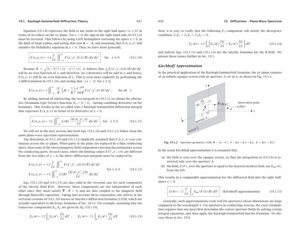
In the practical application of the Rayleigh-Sommerfeld formulas, the xy plane consistsof an infinite opaque screen with an aperture A cut in it, as shown in Fig. 19.1.2.

Fig. 19.1.2 Aperture geometry, with R = |r− r′|, r = xx+ yy + zz, r′ = xx′ + yy′.

In the usual Kirchhoff approximation it is assumed that:

(a) the field is zero over the opaque screen, so that the integration in (19.1.6) is re-stricted only over the aperture A.

(b) the field, E(r′), over the aperture is equal to the (known) incident field, say Einc(r),from the left.

This results in a computable approximation for the diffracted field into the right half-space z > 0,

E(r)= −2∂∂z

∫AEinc(r′)G(R)dS′ (Kirchhoff approximation) (19.1.15)

Generally, such approximations work well for apertures whose dimensions are largecompared to the wavelength λ. For apertures in conducting screens, the exact formula-tion requires that one must first determine the correct aperture fields by solving certainintegral equations, and then apply the Rayleigh-Sommerfeld-Smythe formulas. We dis-cuss these in Sec. 19.9.

19.2. Plane-Wave Spectrum Representation 849

19.2 Plane-Wave Spectrum Representation

The plane-wave spectrum representation builds up a single-frequency propagating waveE(x, y, z) as a linear combination of plane waves e−j(kxx+kyy+kzz).† The only assumptionis that the field must satisfy the wave equation, which becomes the three-dimensionalHelmholtz equation,

(∇2 + k2)E(x, y, z)= 0 , k = ωc=ω√με (19.2.1)

where c = 1/√με is the speed of light in the propagation medium (assumed here to be

homogeneous, isotropic, and lossless.) In solving the Helmholtz equation, one assumesinitially a solution of the form:

E(x, y, z)= E(kx, ky, z)e−jkxxe−jkyy

Inserting this into Eq. (19.2.1) and replacing, ∂x → −jkx and ∂y → −jky, we obtain:(−k2

x − k2y +

∂2

∂z2+ k2

)E(kx, ky, z)= 0

or, defining k2z = k2 − k2

x − k2y, we have:

∂2E(kx, ky, z)∂z2

= −(k2 − k2x − k2

y)E(kx, ky, z)= −k2z E(kx, ky, z)

Its solution describing forward-moving waves (z ≥ 0) is:

E(kx, ky, z)= E(kx, ky)e−jkzz (19.2.2)

where E(kx, ky) is an arbitrary constant in the variable z.If k2

x + k2y < k2, the wavenumber kz is real-valued and the solution describes a

propagating wave. If k2x + k2

y > k2, then kz is imaginary and the solution describes anevanescent wave decaying with distance z. The two cases can be combined into one bydefining kz in terms of the evanescent square-root of Eq. (7.7.9) as follows:

kz =⎧⎪⎨⎪⎩

√k2 − k2

x − k2y , if k2

x + k2y ≤ k2

−j√k2x + k2

y − k2 , if k2x + k2

y > k2

(propagating)

(evanescent)(19.2.3)

and choose the square-root branch, kz = k, when kx = ky = 0. In the evanescent case,we have the decaying solution:

E(kx, ky, z)= E(kx, ky)e−z√k2x+k2

y−k2 , z ≥ 0

Fig. 19.2.1 depicts the two regions on the kxky plane. The complete space dependenceis E(kx, ky)e−jkxx−jkyye−jkzz. The most general solution of Eq. (19.2.1) is obtained by


Fig. 19.2.1 Propagating and evanescent regions on the kxky plane.

adding up such plane-waves, that is, by the spatial two-dimensional inverse Fouriertransform, for z ≥ 0,

E(x, y, z)=∫∞−∞

∫∞−∞E(kx, ky)e−jkxx−jkyye−jkzz

dkx dky(2π)2

(19.2.4)

This is the plane-wave spectrum representation, also known as the angular spectrumrepresentation, see [1415,1419], and some of the original papers [1601,1423–1425].

Because kz is given by Eq. (19.2.3), this solution is composed, in general, of bothpropagating and evanescent modes. Of course, for large z, only the propagating modessurvive. Setting z = 0, we recognize E(kx, ky) to be the spatial Fourier transform of thefield, E(x, y,0), at z = 0 on the xy plane:

E(x, y,0) =∫∞−∞

∫∞−∞E(kx, ky)e−jkxx−jkyy

dkx dky(2π)2

E(kx, ky) =∫∞−∞

∫∞−∞E(x, y,0)ejkxx+jkyy dxdy

(19.2.5)

As in Chap. 3, we may give a system-theoretic interpretation to these results. Defin-ing the “propagation” spatial filter, h(kx, ky, z)= e−jkzz, then Eq. (19.2.2) reads:

E(kx, ky, z)= e−jkzzE(kx, ky)= h(kx, ky, z)E(kx, ky) (19.2.6)

This multiplicative relationship in the wavenumber domain translates into a convo-lutional equation in the space domain. Let h(x, y, z) denote the “impulse response” ofthis filter, that is, the spatial inverse Fourier transform of h(kx, ky, z)= e−jkzz,

h(x, y, z)=∫∞−∞

∫∞−∞e−jkxx−jkyye−jkzz

dkx dky(2π)2

(19.2.7)

then, we may write Eq. (19.2.4) in the convolutional form:

E(x, y, z)=∫∞−∞

∫∞−∞h(x− x′, y − y′, z)E(x′, y′,0)dx′dy′ (19.2.8)

†As always, we use ejωt harmonic time dependence.

19.2. Plane-Wave Spectrum Representation 851

Eq. (19.2.8) is equivalent to the Rayleigh-Sommerfeld formula (19.1.6). Indeed, itfollows from Eq. (D.19) of Appendix D that

h(x− x′, y − y′, z)= −2∂G(R)∂z

= 2∂G(R)∂z′

, G(R)= e−jkR

4πR, R = |r− r′| (19.2.9)

with the understanding that z′ = 0, so that R = √(x− x′)2+(y − y′)2+z2. Thus,

Eq. (19.2.8) takes the form of Eq. (19.1.6) or (19.1.8). The geometry was shown inFig. 19.1.2. We note also that at z = 0, we have h(x−x′, y−y′,0)= δ(x−x′)δ(y−y′).This follows by setting z = 0 into (19.2.7), or from Eq. (D.21) of Appendix D. Thus,Eq. (19.2.8) is consistent at z = 0.

To summarize, the Rayleigh-Sommerfeld and plane-wave spectrum representationsexpress a scalar field E(x, y, z) in terms of its boundary values E(x, y,0) on the xyplane, or in terms of the 2-D Fourier transform E(kx, ky) of these boundary values,

E(x, y, z) = −2∂∂z

∫∫∞−∞

e−jkR

4πRE(x′, y′,0)dx′dy′

= 2

∫∫∞−∞

zR

(jk+ 1

R

)e−jkR


=∫∫∞−∞E(kx, ky)e−jkxx−jkyye−jkzz

dkx dky(2π)2

(19.2.10)

with z ≥ 0 and R =√(x− x′)2+(y − y′)2+z2. For arbitrary z ≷ 0, we have,

E(x, y, z) = ∓2∂∂z

∫∫∞−∞

e−jkR


= 2

∫∫∞−∞

|z|R

(jk+ 1

R

)e−jkR


=∫∫∞−∞E(kx, ky)e−jkxx−jkyye−jkz|z|

dkx dky(2π)2

(19.2.11)

Next, we show that the plane-wave representation (19.2.4) is equivalent to both thetype-1 and the type-2 Rayleigh-Sommerfeld formulas, Eqs. (19.1.6) and (19.1.11). Wenote that Eq. (19.2.6) can be written as follows,

E(kx, ky, z)= e−jkzz · E(kx, ky)= 2jkz ·[e−jkzz

2jkz

]· E(kx, ky)

or,E(kx, ky, z)= 2jkz · G(kx, ky, z)·E(kx, ky) (19.2.12)

where G(kx, ky, z)= e−jkzz/(2jkz) is the 2-D Fourier transform of the Green’s functionG(r)= e−jkr/(4πr), for z ≥ 0. This follows from Eq. (D.11) of Appendix D. The factor2jkz can be associated either with G(kx, ky, z), leading to Eq. (19.1.6), or with E(kx, ky)leading to Eq. (19.1.11),

E(kx, ky, z)= 2jkz · G(kx, ky, z)︸︷︷︸type-1

·E(kx, ky)= 2jkz · E(kx, ky)︸︷︷︸type-2

·G(kx, ky, z) (19.2.13)


We recognize that 2jkz · E(kx, ky) is the 2-D Fourier transform of the z-derivativeof E(x, y, z) at z = 0, indeed, by differentiating (19.2.4), we have,

− 2∂E(x, y, z)

∂z=∫∫∞−∞

2jkz · E(kx, ky) e−jkxx−jkyye−jkzz dkx dky(2π)2(19.2.14)

and at z = 0,

− 2∂E(x, y,0)

∂z=∫∫∞−∞

2jkz · E(kx, ky) e−jkxx−jkyy dkx dky(2π)2(19.2.15)

Thus, the inverse Fourier transform of the product of the transforms G(kx, ky, z)and 2jkz E(kx, ky) in (19.2.13) becomes the convolutional form of Eq. (19.1.11).

19.3 Far-Field Diffraction Pattern

The far-field, or Fraunhofer, diffraction pattern is obtained in the limit of a large radialdistance r of the field observation point from the aperture. It can be derived using eitherthe Rayleigh-Sommerfeld integrals or by applying the stationary-phase approximationto the plane-wave spectrum. We briefly discuss both approaches.

In Eq. (19.2.10), the quantity R = |r − r′| is the distance between the field pointat position r and the aperture point r′. If we assume that the aperture is finite, as inFig. 19.1.2, and we choose r r′, we may approximate R as follows,

R = |r− r′| =√r2 − 2r · r′ + r′2 ≈ r − r · r′

where r is the unit vector in the direction of the observation point r. We have used thisapproximation before in Sec. 15.7, see for example Fig. 15.7.1. The far-field approxima-tion then consists of making the following replacements in Eq. (19.2.10), and assumingthat r λ, or, k 1/r,

zR

(jk+ 1

R

)e−jkR

4πR≈ zr

(jk+ 1

r

)e−jk(r−r·r′)

4πr≈ jk z

re−jkr

4πrejkr·r

′(19.3.1)

where we replaced R ≈ r in the denominators, but kept the approximation R ≈ r− r · r′

in the phase exponential. The unit vector r is uniquely defined by the correspondingpolar and azimuthal angles θ,φ in the direction of r. Thus, z/r = cosθ, and definingthe wavevector k = kr, we have,

k = kr = k(x sinθ cosφ+ y sinθ sinφ+ z cosθ) ⇒kx = k sinθ cosφky = k sinθ sinφkz = k cosθ

(19.3.2)

Since r′ is restricted to the xy plane, we have, ejkr·r′=ekxx′+kyy′ . It follows that Eq. (19.2.10)can be approximated in this limit by,

E(x, y, z)≈ 2jk cosθe−jkr

4πr

∫∞−∞E(x′, y′,0)ekxx

′+kyy′dx′dy′

19.3. Far-Field Diffraction Pattern 853

but the last factor is the 2-D Fourier transform of E(x′, y′,0) evaluated at the directionalwave vector, k = k r,

E(x, y, z)≈ 2jk cosθe−jkr

4πrE(kx, ky)

∣∣∣∣k=kr

(far-field diffraction pattern) (19.3.3)

The factor E(kx, ky) evaluated at k = k r is a function of the angles θ,φ, and rep-resents the essential angular pattern of the diffracted wave. The factor cosθ may beviewed as an obliquity factor.

The same result can be obtained by using the stationary-phase approximation for2-D integrals discussed in Appendix H. Let us rewrite Eq. (19.2.4) in the form,

E(x, y, z)=∫∫∞−∞E(kx, ky)ejϕ(kx,ky)

dkx dky(2π)2

, (19.3.4)

where we defined the phase function,

ϕ(kx, ky)= −k · r = −(kxx+ kyy + kzz) (19.3.5)

The stationary-phase approximation to the integral in (19.3.4) is given by Eq. (H.6),

∫∫∞−∞E(kx, ky)ejϕ(kx,ky)

dkx dky(2π)2

≈ ej(σ+1)τπ42π√|detΦ|

E(k0x, k0

y) ejϕ(k0x,k0

y)

(2π)2(19.3.6)

where k0x, k0

y are the stationary points of the phase function ϕ(kx, ky), that is, the so-lutions of the equations,

∂ϕ∂kx

= 0 ,∂ϕ∂ky

= 0 (19.3.7)

and where Φ is the matrix of second derivatives of ϕ evaluated at the stationary pointsk0x, k0

y, and σ,τ are the algebraic signs of the determinant and trace of Φ, that is,

Φ =

⎡⎢⎢⎢⎢⎢⎣∂2ϕ(k0

x, k0y)

∂kx2

∂2ϕ(k0x, k0

y)∂kx ∂ky

∂2ϕ(k0x, k0

y)∂kx ∂ky

∂2ϕ(k0x, k0

y)∂ky2

⎤⎥⎥⎥⎥⎥⎦ , σ = sign(detΦ) , τ = sign(trΦ) (19.3.8)

Since k2z = k2 − k2

x − k2y, the conditions (19.3.7) become,

∂ϕ∂kx

= −x− z ∂kz∂kx

= −x+ z kxkz= 0 ⇒ k0

x

k0z= xz

∂ϕ∂ky

= −y − z ∂kz∂ky

= −y + z kykz= 0 ⇒ k0

y

k0z= yz

(19.3.9)

Putting these back into k2z = k2 − k2

x − k2y, gives the following solution,

k0x = k

xr, k0

y = kyr, k0

z = kzr, r =

√x2 + y2 + z2 (19.3.10)


or, k0 = kr/r = k r, which is the same as (19.3.2). Therefore, the phase functionevaluated at k0 is, ϕ(k0

x, k0y)= −k0 · r = −k r · r = −kr.

The second derivatives are obtained by differentiating (19.3.9) one more time andevaluating the result at k0, for example,

∂2ϕ∂k2

x= z ∂

∂kx

(kxkz

)= zkz

(1+ k

2xk2z

)∣∣∣∣∣k=k 0

= rk

(1+ x

2

z2

)

and similarly,∂2ϕ∂kx∂ky

= rkxyz2,

∂2ϕ∂k2

y= rk

(1+ y

2

z2

)It follows that, detΦ,σ,τ are,

detΦ = r4

k2z2, σ = τ = 1

and since z > 0, the approximation (19.3.6) yields the same answer as (19.3.3),

E(x, y, z)≈ ej(σ+1)τπ42π√|detΦ|

E(k0x, k0

y)ejϕ(k0x,k0

y)

(2π)2= ej(1+1) π4

2π√r4

k2z2

E(k0x, k0

y)e−jkr

(2π)2

or,

E(x, y, z)= jk zre−jkr

2πrE(k0

x, k0y)= 2jk cosθ

e−jkr

4πrE(k0

x, k0y)

19.4 One-Dimensional Apertures

The plane-wave spectrum representations and the Rayleigh-Sommerfeld diffraction for-mulas apply also to the special case of one-dimensional line sources and apertures, suchas infinitely long narrow slits or strips, as shown for example in Fig. 19.4.1.

Fig. 19.4.1 Slit aperture with infinite length in the y-direction.

Specifically, we will assume that the one-dimensional aperture is along the x-directionand the fields, E(x, z), depend only on the x, z coordinates and have no dependence onthe y-coordinate. We recall from Eqs. (D.22) and (D.32) of Appendix D that the 2-D

19.4. One-Dimensional Apertures 855

outgoing Green’s function can be derived by integrating out the y-variable of the 3-DGreen’s function, that is,

G2(x− x′, z)= − j4H(2)0 (kρ)=

∫∞−∞

e−jkR

4πRdy′ (19.4.1)

where, ρ = √(x− x′)2+z2 and R = √(x− x′)2+(y − y′)2+z2.Since E(x′, y′,0) does not depend on y′, we may integrate out the y′ variable in

Eq. (19.1.10) and use Eq. (19.4.1) to obtain the one-dimensional-aperture version of theRayleigh-Sommerfeld diffraction integral, for z > 0,

E(x, z)= −2∂∂z

∫∞−∞E(x′,0)G2(x− x′, z)dx′ (1-D apertures) (19.4.2)

The corresponding 1-D plane-wave spectrum representation can be derived with thehelp of the Weyl representation of the G2 Green’s function derived in Eq. (D.30) of Ap-pendix D, that is,

G2(x, z)= − j4H(2)0

(k√x2 + z2

) = ∫∞−∞

e−jkxx e−jkz|z|

2jkzdkx2π

(19.4.3)

which implies that, for z ≥ 0,

− 2∂G2(x, z)

∂z=∫∞−∞e−jkxx e−jkzz

dkx2π

(19.4.4)

with kz defined as in Eq. (D.27) in terms of the evanescent square root,

kz =⎧⎪⎨⎪⎩

√k2 − k2

x , if |kx| < k−j√k2x − k2 , if |kx| > k

(19.4.5)

It follows that the convolutional equation (19.4.2) can also be written as the inverse1-D Fourier transform,

E(x, z)=∫∞−∞E(kx) e−jkxx e−jkzz

dkx2π

(19.4.6)

where E(kx) is the 1-D Fourier transform of E(x,0) at z = 0,

E(kx) =∫∞−∞E(x,0) e−jkxx dx

E(x,0) =∫∞−∞E(kx) e−jkxx

dkx2π

(19.4.7)

ReplacingG2 in terms of the Hankel function and noting the differentiation property,dH(2)0 (z)/dz = −H(2)1 (z), we may summarize the above results as follows,

E(x, z) = j2

∂∂z

∫∞−∞H(2)0 (kρ)E(x′,0)dx′

= − j2

∫∞−∞

kzρH(2)1 (kρ)E(x′,0)dx′

=∫∞−∞E(kx) e−jkxx e−jkzz

dkx2π

z ≥ 0

ρ =√(x− x′)2+z2

(19.4.8)


The far-field approximation easily follows from (19.4.8), for large r = √x2 + z2,

E(x, z)≈ ej π4 cosθ

√k

2πre−jkr E(k0

x) (far-field approximation) (19.4.9)

where k0x = kx/r = k sinθ, k0

z = kz/r = k cosθ, cosθ = z/r. Eq. (19.4.9) can bederived either by applying the stationary-phase method to the one-dimensional Fourierintegral (19.4.6), that is, Eq. (H.4) of Appendix H, or, by using the following asymptoticexpression for the Hankel function H(2)1 in (19.4.8),

H(2)1 (kρ)≈√

2

πkρe−j(kρ−

3π4 ) , for large ρ

and replacing the ρ in the exponential e−jkρ by the approximation,

ρ =√(x− x′)2+z2 =

√r2 − 2xx′ + x′2 ≈ r − x

rx′

and also replacing ρ by r in the other factors of (19.4.8).In both the 3-D and 2-D cases, the radial dependence of the far field describes an out-

going spherical or cylindrical wave, while the angular pattern is given by the product ofthe obliquity factor cosθ and the spatial Fourier transform of the aperture distributionevaluated at the wavenumber k = k r.

19.5 Plane-Wave Spectrum–Vector Case

Next, we discuss the vector case for electromagnetic fields. To simplify the notation,we define the two-dimensional transverse vectors r⊥ = xx + yy and k⊥ = xkx + yky,as well as the transverse gradient ∇∇∇⊥ = x∂x + y∂y, so that the full three-dimensionalgradient is,

∇∇∇ = x∂x + y∂y + z∂z =∇∇∇⊥ + z∂z

In this notation, Eq. (19.2.6) reads, E(k⊥, z)= h(k⊥, z)E(k⊥), with h(k⊥, z)= e−jkzz.The plane-wave spectrum representations (19.2.4) and (19.2.8) now are,†

E(r⊥, z) =∫∞−∞E(k⊥) e−jkzz e−jk⊥·r⊥

d2k⊥(2π)2

=∫∞−∞E(r⊥′,0)h(r⊥ − r⊥′, z)d2r⊥′

(19.5.1)

for z ≥ 0, where

E(k⊥)=∫∞−∞ejk⊥·r⊥ E(r⊥,0)d2r⊥ (19.5.2)

and

†where the integral sign represents double integration; note also that in the literature one often sees thenotation k‖, r‖, with the subscript ‖meaning “parallel” to the interface, whereas our notation k⊥, r⊥ means“perpendicular” to z.

19.5. Plane-Wave Spectrum–Vector Case 857

h(r⊥, z)=∫∞−∞e−jkzz e−jk⊥·r⊥

d2k⊥(2π)2

= −2∂∂z

(e−jkr

4πr

), r =

√r⊥·r⊥ + z2 (19.5.3)

In the vectorial case, E(r⊥, z) is replaced by a three-dimensional field, which can bedecomposed into its transverse x, y components and its longitudinal part along z:

E = xEx + yEy︸︷︷︸transverse part

+zEz ≡ E⊥ + zEz

The plane-wave spectrum representations apply separately to each component of Eand H, and can be written vectorially as follows, for z ≥ 0,

E(r⊥, z) =∫∞−∞

E(k⊥) e−jkzz e−jk⊥·r⊥d2k⊥(2π)2

H(r⊥, z) =∫∞−∞

H(k⊥) e−jkzz e−jk⊥·r⊥d2k⊥(2π)2

(19.5.4)

where E(k⊥), H(k⊥) are the 2-D Fourier transforms,

E(k⊥) =∫∞−∞ejk⊥·r⊥ E(r⊥,0)d2r⊥

H(k⊥) =∫∞−∞ejk⊥·r⊥ H(r⊥,0)d2r⊥

(19.5.5)

Because E must satisfy the source-free Gauss’s law, ∇∇∇ · E = 0, this imposes certainconstraints among the Fourier components, E(k⊥), that must be taken into account inwriting (19.5.4). Indeed, we have from (19.5.4)

∇∇∇ · E = −j∫∞−∞

k · E(k⊥) e−jkzz e−jk⊥·r⊥d2k⊥(2π)2

= 0

which requires that k · E(k⊥)= 0. Separating this into its transverse and longitudinalparts, we have:

k · E = k⊥ · E⊥ + kzEz = 0 , or,

Ez(k⊥)= −k⊥ · E⊥(k⊥)kz

= −kxEx(k⊥)+kyEy(k⊥)kz

(19.5.6)

It follows that the Fourier vector E(k⊥) must have the form:

E(k⊥)= E⊥(k⊥)+z Ez(k⊥)= E⊥(k⊥)−zk⊥ · E⊥(k⊥)

kz(19.5.7)

and it is expressible only in terms of its transverse components E⊥(k⊥). Thus, thecorrect plane-wave spectrum representation for the E-field as well as that for the H-


field become in the vector case, for z ≥ 0,

E(r⊥, z) =∫∞−∞

[E⊥(k⊥)−z

k⊥ · E⊥(k⊥)kz

]e−jkzz e−jk⊥·r⊥

d2k⊥(2π)2

H(r⊥, z) = 1

ηk

∫∞−∞

k×[

E⊥(k⊥)−zk⊥ · E⊥(k⊥)

kz


d2k⊥(2π)2

(19.5.8)

where, k = k⊥+ zkz = xkx+yky+ zkz. The magnetic field was obtained from Faraday’slaw, ∇∇∇× E = −jωμH . Replacing, ωμ = kη, since k = ω√με and η = √

μ/ε, we have,H =∇∇∇×E /(−jkη), which leads to the above expression for H by bringing the gradient∇∇∇ inside the Fourier integral for E, and replacing it by∇∇∇ → −jk.

The plane-wave Fourier components for E and H form a right-handed vector triplettogether with the vector k,

E(k⊥) = E⊥(k⊥)−zk⊥ · E⊥(k⊥)

kz

H(k⊥) = 1

ηkk×

[E⊥(k⊥)−z

k⊥ · E⊥(k⊥)kz

]= 1

ηkk× E(k⊥)

(19.5.9)

Albeit complex-valued because of Eq. (19.2.3), the normalized vector k = k/k can bethought of as a unit vector, indeed, satisfying, k · k = k2

x + k2y + k2

z = k2, or, k · k = 1.It follows from (19.5.9), that k·H(k⊥)= 0 and k×H(k⊥)= −k E(k⊥)/η = −ωε E(k⊥),

which imply that Eqs. (19.5.8) satisfy the remaining Maxwell equations, that is,∇∇∇·H = 0and∇∇∇×H = jωεE, in the right half-space z ≥ 0.

We could equally well have started with the tangential components of the magneticfield on the aperture, H⊥(r⊥′,0), and the corresponding Fourier transform, H⊥(k⊥),and have used the constraint∇∇∇ ·H = 0, or, k⊥ · H⊥(k⊥)+kzHz(k⊥)= 0 , to obtain thefollowing alternative plane-wave spectrum representation, with the electric field derivedfrom, jωεE =∇∇∇×H, or, E = (η/jk)∇∇∇×H, for z ≥ 0,

H(r⊥, z) =∫∞−∞

[H⊥(k⊥)−z

k⊥ · H⊥(k⊥)kz


d2k⊥(2π)2

E(r⊥, z) = −ηk∫∞−∞

k×[

H⊥(k⊥)−zk⊥ · H⊥(k⊥)

kz


d2k⊥(2π)2

(19.5.10)

The plane-wave Fourier components still form a right-handed triplet with k,

H(k⊥) = H⊥(k⊥)−zk⊥ · H⊥(k⊥)

kz

E(k⊥) = −ηk k×[

H⊥(k⊥)−zk⊥ · H⊥(k⊥)

kz

]= −η

kk× H(k⊥)

(19.5.11)

Eqs. (19.5.11) are entirely equivalent to (19.5.9), hence (19.5.10) are equivalent to(19.5.8). Eqs. (19.5.10) could also be obtained quickly from (19.5.8) by a duality trans-formation, that is, E → H, H → −E, η→ η−1.

19.5. Plane-Wave Spectrum–Vector Case 859

Example 19.5.1: Oblique Plane Wave. Here, we show that the plane-wave spectrum methodcorrectly generates an ordinary plane wave from its transverse values at an input plane.Consider a TM electromagnetic wave propagating at an angle θ0 with respect to the z axis,as shown in the figure below. The electric field at an arbitrary point, and its transversepart evaluated on the plane z′ = 0, are given by

E(r⊥, z) = E0(x cosθ0 − z sinθ0)e−j(k0xx+k0

zz)

E⊥(r⊥′,0) = xE0 cosθ0 e−jk0xx′ = xE0 cosθ0e−jk

0⊥·r⊥′

k0x = k sinθ0 , k0

y = 0 , k0z = k cosθ0

k0⊥ = xk0

x + yk0y = xk sinθ0

It follows that the spatial Fourier transform of E⊥(r⊥′,0) will be

E⊥(k⊥,0)=∫∞−∞

xE0 cosθ0 e−jk0⊥·r⊥′ ejk⊥·r⊥

′d2r⊥′ = xE0 cosθ0(2π)2δ(k⊥ − k0

⊥)

Then, the integrand of Eq. (19.5.8) becomes

E⊥ − zk⊥ · E⊥kz

= E0(x cosθ0 − z sinθ0)(2π)2δ(k⊥ − k0⊥)

and Eq. (19.5.8) gives

E(r⊥, z) =∫ ∞−∞E0(x cosθ0 − z sinθ0)(2π)2δ(k⊥ − k0

⊥)e−jkzz e−jk⊥·r⊥d2k⊥(2π)2

= E0(x cosθ0 − z sinθ0)e−j(k0xx+k0

zz)

which is the correct expression for the plane wave. For a TE wave a similar result holds. ��

One-Dimensional Apertures

As in Sec. 19.4, we assume that there is no y-dependence in the fields (see Fig. 19.4.1for the geometry). The 2-D Fourier transforms of the 2-D aperture fields reduce to 1-DFourier transforms of 1-D fields:

E⊥(kx, ky) =∫∞−∞

E⊥(x,0)e−jkxx−jkyy dxdy

=∫∞−∞

E⊥(x,0)ejkxx dx ·∫∞−∞ejkydy = E(kx)·2πδ(ky)

The δ(ky) factor effectively sets ky = 0 in the 2-D expressions and eliminates theky integrations, replacing (19.5.8) by,

E(x, z) =∫∞−∞

[E⊥(kx)−z

kx Ex(kx)kz

]e−jkzz e−jkxx

dkx2π

H(x, z) = 1

ηk

∫∞−∞

k×[

E⊥(kx)−zkx Ex(kx)

kz

]e−jkzz e−jkxx

dkx2π

(19.5.12)


where now, k = k⊥ + zkz = xkx + zkz, and hence, the constraint, k · E = 0, implies,

Ez = −k⊥·E⊥kz

= −kx Exkz

(19.5.13)

We may rewrite (19.5.12) more explicitly in terms of the transverse Ex, Ey components,

E(x, z) =∫∞−∞

[yEy(kx)+ 1

kz(xkz − zkx)Ex(kx)

]e−jkxx−jkzz

dkx2π

H(x, z) = 1

ηk

∫∞−∞

[(zkx − xkz)Ey(kx)+y

k2

kzEx(kx)

]e−jkxx−jkzz

dkx2π

(19.5.14)

Thus, the Fourier components of the magnetic field are,

Hx = − kzηk Ey , Hy = kηkz

Ex , Hz = kxηk

Ey (19.5.15)

19.6 Far-Field Approximation, Radiation Pattern

The far-field approximation for the vector case is easily obtained by applying Eq. (19.3.3)to each component of the E,H fields, that is, for large r,

E(r)≈ 2jk cosθe−jkr

4πrE(k⊥)

∣∣∣∣k=kr

(far-field radiation pattern) (19.6.1)

and similarly for H. Since k · E = 0 and k = k r, it follows that, r · E(r)= 0, thus, the farfield has no radial component. The azimuthal and polar components are easily workedout from (19.6.1) to be,

Eφ = 2jke−jkr

4πrcosθ

[Ey cosφ− Ex sinφ

]Eθ = 2jk

e−jkr

4πr[Ex cosφ+ Ey sinφ

]H = 1

ηr× E ⇒ Hφ = 1

ηEθ , Hθ = − 1

ηEφ

(19.6.2)

These are the same as Eqs. (18.4.10) and (18.4.12) of Chap. 18, if we recognize thatthe quantity f(θ,φ) in those equations is nothing but f(θ,φ)= E⊥(k⊥) evaluated atk = k r. In a similar fashion, we can show that the far-field approximation based on(19.5.10) is equivalent to (18.4.11), where now we have, g(θ,φ)= H⊥(k⊥).

The cosθ factor is an obliquity factor and is sometimes referred to as an elementfactor [1447]. The factors,

[Ey cosφ− Ex sinφ

]and

[Ex cosφ+ Ey sinφ

], are referred

to as pattern space factors.For the 1-D case described by Eq. (19.5.12), the far-field approximation follows by

applying the scalar result (19.4.9) to each component, that is, for large r = √x2 + z2,

E(r,θ)≈ ej π4 cosθ

√k

2πre−jkr E(k0

x) (far-field approximation) (19.6.3)

19.7. Radiated and Reactive Power, Directivity 861

where, k0x = k sinθ, k0

z = k cosθ, cosθ = z/r. Resolving these into the cylindricalcoordinate directions, r, θθθ, y, shown in Fig. 19.4.1, we have, E = θθθEθ + yEy,

Ey(r,θ) = ejπ4

√k

2πre−jkr cosθ Ey(k0

x)

Eθ(r,θ) = ejπ4

√k

2πre−jkr Ex(k0

x)

(19.6.4)

For the magnetic field, we have, H = r× E /η = (y Eθ − θθθ Ey)/η,

Hθ(r,θ) = − 1

ηEy = − 1

ηej

π4

√k

2πre−jkr cosθ Ey(k0

x)

Hy(r,θ) = 1

ηEθ = 1

ηej

π4

√k

2πre−jkr Ex(k0

x)

(19.6.5)

19.7 Radiated and Reactive Power, Directivity

The z-component of the Poynting vector at the z = 0 plane is given by,

Sz = 1

2E(r⊥,0)×H∗(r⊥,0)·z (19.7.1)

The total power Prad transmitted through the aperture at z = 0, and radiated into theright half-space, can be obtained by integrating the real part, Re[Sz], over the aperture.Similarly, the integral of the imaginary part, Im[Sz], gives the reactive power Preact atthe aperture. Thus, we have,

Prad + jPreact =∫∞−∞Sz d2r⊥ = 1

2

∫∞−∞

E(r⊥,0)×H∗(r⊥,0)·z d2r⊥ (19.7.2)

Applying the vectorial version of Parseval’s identity, we may express Eq. (19.7.2) asan integral in the wavenumber domain of the corresponding 2-D Fourier transforms E, Hof E,H, which are defined in Eq. (19.5.8). Thus, we find,

Prad + jPreact = 1

2

∫∞−∞

E(r⊥,0)×H∗(r⊥,0)·z d2r⊥

= 1

2

∫∞−∞

E(k⊥)×H∗(k⊥)·z d2k⊥

(2π)2

(19.7.3)

But the plane-wave Fourier components satisfy, H = k× E /ηk, where k = k⊥ + zkz.The vector k⊥ is real-valued but kz becomes imaginary in the evanescent part of theintegral. Therefore, we may write, k∗ = k⊥+zk∗z = k+z(k∗z −kz). Using the constraint,k · E = 0, which implies, k∗ · E = Ez(k∗z − kz), it follows that,

E× H∗ · z = 1

ηkE× (k∗ × E

∗)·z = 1

ηk[k∗ |E|2 − E

∗ (k∗ · E)] · z

= 1

ηk[k∗z |E|2 − E∗z Ez(k∗z − kz)

] = 1

ηk[k∗z |E⊥|2 + kz|Ez|2

]


Thus, Eq. (19.7.3) becomes,

Prad + jPreact = 1

2ηk

∫∞−∞[k∗z |E⊥|2 + kz|Ez|2

] d2k⊥(2π)2

(19.7.4)

Splitting the integration over the visible/propagating region, |k⊥| =√k2x + k2

y ≤ k,

and over the invisible/evanescent region, |k⊥| =√k2x + k2

y > k, and noting that kz isreal over the former, and imaginary, over the latter region, we may separate Prad, Preact,

Prad + jPreact = 1

2ηk

[∫|k⊥|≤k

+∫|k⊥|>k

][k∗z |E⊥|2 + kz|Ez|2

] d2k⊥(2π)2

Prad = 1

2η

∫|k⊥|≤k

[|E⊥|2 + |Ez|2] kzk d2k⊥(2π)2

Preact = 1

2η

∫|k⊥|>k

[|E⊥|2 − |Ez|2] jkzk d2k⊥(2π)2

kz =√k2 − |k⊥|2

jkz =√|k⊥|2 − k2

(19.7.5)

In Sec. 18.6, we assumed that the transverse aperture fields were Huygens sources,that is, H⊥(r⊥,0)= z×E⊥(r⊥,0)/η. Under this assumption, the radiated power is givenapproximately by,

Prad = 1

2

∫∞−∞

Re[E⊥(r⊥,0)×H∗⊥(r⊥,0)

] · z d2r⊥

= 1

2η

∫∞−∞

∣∣E⊥(r⊥,0)∣∣2 d2r⊥ = 1

2η

∫∞−∞

|E⊥|2 d2k⊥(2π)2

(19.7.6)

where we used Parseval’s identity in the last two integrals. Eq. (19.7.6) approximates(19.7.5) for large apertures [19]. Indeed, E⊥ is typically highly peaked in the forwarddirection, k⊥ = 0, or, kz = k, and hence, Ez = −k⊥ · E⊥/kz is small compared to E⊥ in(19.7.5). Thus, the two expressions will agree, if we also assume that the contribution ofthe invisible/evanescent region, |k⊥| > k, in (19.7.6) is small. However, such assumptionis not warranted in the so-called super-directive apertures where a huge amount ofreactive power resides in the invisible region.

An alternative way of calculating the radiated power is by integrating the radialcomponent of the Poynting vector over a hemisphere of very large radius in the righthalf-space. At large radial distances, we may use the radiated fields given in (19.6.1),

Erad(r)= 2jk cosθe−jkr

4πrE(k0

⊥)∣∣∣∣

k0=kr, Hrad(r)= 1

ηr× Erad (19.7.7)

The corresponding Poynting vector has only a radial component, since, r · Erad = 0,

PPP = 1

2Re[Erad ×H∗rad

] = 1

2ηRe[Erad × (r× E∗rad)

] = r1

2η|Erad|2 = rPr (19.7.8)

Using spherical coordinates, the net power transmitted through the right-half hemi-sphere of radius r will be given as follows,

19.7. Radiated and Reactive Power, Directivity 863

Prad =∫Pr dS =

∫ π/20

∫ 2π

0Pr r2 sinθdθdφ =

∫ π/20

∫ 2π

0

1

2η|Erad|2 r2 sinθdθdφ

=∫ π/2

0

∫ 2π

0

1

2η

∣∣∣∣∣2jk cosθe−jkr

4πrE(k0

⊥)

∣∣∣∣∣2

r2 sinθdθdφ

= 1

2η(2π)2

∫ π/20

∫ 2π

0

∣∣E(k0⊥)∣∣2 k2 cos2 θ sinθdθdφ

Changing variables from θ,φ to kx = k sinθ cosφ, ky = k sinθ sinφ, and notingthat, dkx dky = k2 cosθ sinθdθdφ, and, kz = k cosθ, it follows that the last integralcan be transformed into that of Eq. (19.7.5).

The directivity in direction, θ,φ, is defined as follows in terms of the radiationintensity (radiated power per unit solid angle), dP/dΩ = r2dP/dS = r2Pr ,

D(θ,φ)= dP/dΩPrad/4π

= 4πr2PrPrad

= k2

πcos2 θ

∣∣E(k0⊥)∣∣2∫

|k⊥|≤k

∣∣E(k⊥)∣∣2 kz

kd2k⊥(2π)2

(19.7.9)

Assuming that the maximum directivity is in the forward direction, k⊥ = 0, we have,

Dmax = 4πλ2

∣∣E⊥(0)∣∣2∫

|k⊥|≤k

∣∣E(k⊥)∣∣2 kz

kd2k⊥(2π)2

(19.7.10)

where we replaced, k2/π = 4π/λ2, and∣∣E(0)

∣∣2 = ∣∣E⊥(0)∣∣2

, since, Ez = −k⊥·E⊥/kz =0, at k⊥ = 0. By comparison, the approximate expression (18.6.10) in Sec. 18.6 was,

Dmax = 4πλ2

∣∣E⊥(0)∣∣2∫∞

−∞

∣∣E⊥(k⊥)∣∣2 d2k⊥(2π)2

= 4πλ2

∣∣∣∣∫∞−∞ E⊥(r⊥,0)d2r⊥∣∣∣∣2

∫∞−∞

∣∣E⊥(r⊥,0)∣∣2 d2r⊥

(19.7.11)

Quite similar expressions hold also in the 1-D aperture case. The total radiated andreactive powers (per unit y-length) are defined by integrating the z-component of thePoynting vector over the x-aperture only. This gives,

P′rad + jP′react =∫∞−∞Sz dx = 1

2ηk

∫∞−∞[k∗z |E⊥|2 + kz|Ez|2

] dkx2π

(19.7.12)

where the prime means “per unit y-length.” Then, (19.7.12) separates as,

P′rad =1

2η

∫|kx|≤k

[|E⊥|2 + |Ez|2] kzk dkx2π

P′react =1

2η

∫|kx|>k

[|E⊥|2 − |Ez|2] jkzk dkx2π

kz =√k2 − k2

x

jkz =√k2x − k2

(19.7.13)


It is convenient to rewrite these in a form that explicitly separates the TE and TMcomponents, that is, Ey and Hy, Using Eqs. (19.5.15), we find,

P′rad =1

2η

∫|kx|≤k

[|Ey|2 + |ηHy|2] kzk dkx2π

P′react =1

2η

∫|kx|>k

[|Ey|2 − |ηHy|2] jkzk dkx2π

kz =√k2 − k2

x

jkz =√k2x − k2

(19.7.14)

Indeed, using Eqs. (19.5.15), we have in the visible region, |kx| ≤ k,

|E|2 = |Ex|2+|Ey|2+|Ez|2 = |Ey|2+|Ex|2+ k2xk2z|Ex|2 = |Ey|2+ k

2

k2z|Ex|2 = |Ey|2+|ηHy|2

Similarly, in the invisible region, |kx| > k, we have noting that |kz|2 = k2x − k2,

|E⊥|2 − |Ez|2 = |Ey|2 + |Ex|2 − k2x

|kz|2 |Ex|2 = |Ey|2 − k

2

k2z|Ex|2 = |Ey|2 − |ηHy|2

The same expression for P′rad can also be obtained by integrating the radial com-ponent Pr of the Poynting vector over a semi-cylindrical surface of large radius r andusing the radiation fields (19.6.3). Fig. 19.7.1 illustrates the surface conventions in the1-D and 2-D cases.

Fig. 19.7.1 Radiated power from 2-D and 1-D apertures.

The directivity may be defined in terms of the power density through the cylindricalsurface dS = rdθdy, that is,,

dP = Pr rdθdyor, with P′ = dP/dy, using (19.6.3),

dPdθdy

= dP′

dθ= rPr = r 1

2η|Erad|2 = r 1

2η

∣∣∣∣∣∣ej π4 cosθ

√k

2πre−jkr E(k0

x)

∣∣∣∣∣∣2

which gives for the directivity towards the θ-direction,

D(θ)= dP′/dθP′rad/2π

= k cos2 θ∣∣E(k0

x)∣∣2∫ k

−k

∣∣E(kx)∣∣2 kz

kdkx2π

(19.7.15)

19.8. Smythe Diffraction Formulas 865

where k0x = k sinθ. We note that the denominator P′rad/2π in the above definition

represents the radiation intensity in the ideal cylindrically-isotropic case, that is,(dP′

dθ

)isotropic

= P′rad

2π

If the maximum directivity is towards the forward direction, θ = 0, or, k0x = 0, then,

Ez = 0, and we find the following expression for the maximum directivity, expressiblealso in terms of the TE and TM components,

Dmax = k∣∣E⊥(0)

∣∣2∫ k−k

∣∣E(kx)∣∣2 kz

kdkx2π

= 2πλ

∣∣Ey(0)∣∣2 + ∣∣ηHy(0)∣∣2∫ k−k[|Ey(kx)|2 + |ηHy(kx)|2] kzk dkx

2π(19.7.16)

Finally, had we assumed that the aperture fields were Huygens sources, the maximumdirectivity would be given by the analogous expression to (19.7.11),

Dmax = 2πλ

∣∣E⊥(0)∣∣2∫∞

−∞

∣∣E⊥(kx)∣∣2 dkx

2π

= 2πλ

∣∣∣∣∫∞−∞ E⊥(x,0)dx∣∣∣∣2

∫∞−∞

∣∣E⊥(x,0)∣∣2 dx

(19.7.17)

For a finite-aperture of lengthL, extending over−L/2 ≤ x ≤ L/2, Eq. (19.7.17) is max-imized when the aperture distribution E⊥(x,0) is uniform, resulting in the maximumvalue, Dmax = 2πL/λ. This is the 1-D version of the 2-D result, Dmax = 4πA/λ2, foruniform apertures that we derived in Sec. 18.6, under the approximation of Eq. (19.7.6).

19.8 Smythe Diffraction Formulas

The plane-wave representations Eqs. (19.5.8) or Eq. (19.5.10), can also be written convolu-tionally in terms of the transverse components, E⊥(r⊥′,0),H⊥(r⊥′,0), on the z = 0 aper-ture plane. The resulting Rayleigh-Sommerfeld type formulas are known as Smythe’sformulas [1328].

From the Weyl representations (D.18) and (D.20) of Appendix D, we have withG(r)=e−jkr/4πr, and r = |r| = √x2 + y2 + z2, and for z ≥ 0,

−2∂G∂z

=∫∞−∞e−jkzz e−jk⊥·r⊥

d2k⊥(2π)2

, −2∇∇∇⊥G =∫∞−∞

k⊥kze−jkzz e−jk⊥·r⊥

d2k⊥(2π)2

that is, we have the 2-D Fourier transforms with respect to r⊥,

G(k⊥, z)= e−jkzz

2jkz, −2

∂G∂z

= e−jkzz , −2%∇∇∇⊥G = k⊥kze−jkzz (19.8.1)

We observe that in (19.5.8) the following products of Fourier transforms (in k⊥)appear, which will become convolutions in the r⊥ domain:


E⊥(k⊥)·e−jkzz = E⊥(k⊥)·(−2∂G∂z

)

E⊥(k⊥)·(

k⊥kze−jkzz

)= E⊥(k⊥)·

(−2%∇∇∇⊥G)

E(r⊥, z)=∫∞−∞

[E⊥(k⊥)·

(−2∂G∂z

)− z

[E⊥(k⊥)·

(−2%∇∇∇⊥G)]

]e−jk⊥·r⊥

d2k⊥(2π)2

It follows that (19.5.8) can be written convolutionally in the form:

E(r⊥, z)= −2

∫∞−∞

[E⊥(r⊥′,0)

∂G(R)∂z

− z(

E⊥(r⊥′,0)·∇∇∇⊥G(R))]

d2r⊥′ (19.8.2)

where hereG(R)= e−jkR/4πRwithR = |r−r ′| and z′ = 0, that is,R = √|r⊥ − r⊥′|2 + z2.Because E⊥(r⊥′,0) does not depend on r, it is straightforward to verify using some vectoridentities that,

z (∇∇∇⊥G · E⊥)−E⊥∂G∂z

=∇∇∇× (z× E⊥G) (19.8.3)

This gives rise to Smythe’s formulas for the electric and magnetic fields, for z ≥ 0,

E(r⊥, z) = 2∇∇∇×∫∞−∞

z× E⊥(r⊥′,0)G(R)d2r⊥′

H(r⊥, z) = 2jηk∇∇∇×

(∇∇∇×

∫∞−∞

z× E⊥(r⊥′,0)G(R)d2r⊥′) (Smythe) (19.8.4)

with G(R)= e−jkR/4πR, and R = √|r⊥ − r⊥′|2 + z2. In a similar fashion, we obtain theSmythe formulas for the alternative representation of Eq. (19.5.10), which can also beobtained by applying a duality transformation to (19.8.4),

H(r⊥, z) = 2∇∇∇×∫∞−∞

z×H⊥(r⊥′,0)G(R)d2r⊥′

E(r⊥, z) = 2ηjk∇∇∇×

(∇∇∇×

∫∞−∞

z×H⊥(r⊥′,0)G(R)d2r⊥′) (19.8.5)

Perhaps a faster way of deriving Eqs. (19.8.4) is as follows. Working in the wavenum-ber domain and using the constraint, k · E = kzEz + k⊥ · E⊥ = 0, and some vectoridentities, we obtain,

k×(z×E⊥)= k×(z×E)= (k·E)z−(k·z)E = −Ekz ⇒ E(k⊥)= −k× (z× E⊥(k⊥))

kz

Recalling that, G(k⊥, z)= e−jkzz/(2jkz), is the 2-D Fourier transform of the Green’sfunction G(r)= e−jkr/(4πr), for z ≥ 0, we can write the propagation filter in the form,

h(k⊥, z)= e−jkzz = 2jkz ·[e−jkzz

2jkz

]= 2jkz · G(k⊥, z) (19.8.6)


Then, the Fourier transform of the propagated field becomes,

E(k⊥, z)= E(k⊥)e−jkzz = E(k⊥)·2jkz · G(k⊥, z)= −k× (z× E⊥(k⊥))

kz·2jkz · G(k⊥, z)

or,E(k⊥, z)= −2 jk× (z× E⊥(k⊥)

) · G(k⊥, z) (19.8.7)

Eq. (19.8.4) follows immediately from this by taking inverse Fourier transforms ofboth sides and replacing −jk by∇∇∇.

Connection to Franz Formulas

The Smythe formulas can be also derived more directly by using the Franz formulas(18.10.13) and making use of the extinction theorem as we did in Sec. 19.1 in the dis-cussion of the Rayleigh-Sommerfeld formula.

Assuming z > 0, and applying (18.10.13) to the closed surface S+ S∞ of Fig. 19.1.1,and dropping the S∞ term, it follows that the left-hand side of (18.10.13) will be zeroif the point r is not in the right half-space. In particular, it will be zero when evaluatedat the reflected point r− = r⊥ − zz in the left half-space. To simplify the notation, wedefine the transverse electric and magnetic vector potentials:†

F(r) = 2

∫∞−∞[z× E⊥(r⊥′,0)

]G(R)d2r⊥′

A(r) = 2

∫∞−∞[z×H⊥(r⊥′,0)

]G(R)d2r⊥′

(19.8.8)

where we took S to be the xy plane with the unit vector n = z, and G(R)= e−jkR/4πR,and R = √|r⊥ − r⊥′|2 + z2. Then, the Franz formulas, Eqs. (18.10.13) and (18.10.14), canbe written as follows, after setting ωμ = kη and ωε = k/η,

E(r) = 1

2

ηjk∇∇∇× (∇∇∇× A)+ 1

2∇∇∇× F

H(r) = 1

2

−1

jkη∇∇∇× (∇∇∇× F)+ 1

2∇∇∇× A

(19.8.9)

Noting that F,A are transverse and using some vector identities and the decompo-sition∇∇∇ = ∇∇∇⊥ + z∂z, we may rewrite the above in a form that explicitly separates thetransverse and longitudinal parts, so that if r is in the right half-space:

E(r) = 1

2

ηjk[∇∇∇⊥(∇∇∇⊥ · A)−∇∇∇2A

]+ 1

2z× ∂zF︸︷︷︸

transverse

+ 1

2

ηjk[z∂z(∇∇∇⊥ · A)

]+ 1

2∇∇∇⊥ × F︸︷︷︸

longitudinal

H(r) = 1

2

−1

jkη[∇∇∇⊥(∇∇∇⊥ · F)−∇∇∇2F

]+ 1

2z× ∂zA︸︷︷︸

transverse

+ 1

2

−1

jkη[z∂z(∇∇∇⊥ · F)

]+ 1

2∇∇∇⊥ × A︸︷︷︸

longitudinal

(19.8.10)

†In the notation of Eq. (18.10.12), we have F = −2Ams/ε and A = 2A s/μ.


where we used the identity,

∇∇∇× (∇∇∇× A)=∇∇∇(∇∇∇ · A)−∇∇∇2A =∇∇∇⊥(∇∇∇⊥ · A)−∇∇∇2A︸︷︷︸transverse

+ z∂z(∇∇∇⊥ · A)︸︷︷︸longitudinal

If r is chosen to be the reflected point r− in the left half-space, then G− = G and thevectors F,A remain the same, but the gradient with respect to r− is now∇∇∇− =∇∇∇⊥− z∂z,arising from the replacement z→ −z. Thus, replacing ∂z → −∂z in (19.8.10) and settingthe result to zero, we have:

0 = 1

2

ηjk[∇∇∇⊥(∇∇∇⊥ · A)−∇∇∇2A

]− 1

2z× ∂zF︸︷︷︸

transverse

+ 1

2

ηjk[−z∂z(∇∇∇⊥ · A)

]+ 1

2∇∇∇⊥ × F︸︷︷︸

longitudinal

0 = 1

2

−1

jkη[∇∇∇⊥(∇∇∇⊥ · F)−∇∇∇2F

]− 1

2z× ∂zA︸︷︷︸

transverse

+ 1

2

−1

jkη[−z∂z(∇∇∇⊥ · F)

]+ 1

2∇∇∇⊥ × A︸︷︷︸

longitudinal

(19.8.11)Separating (19.8.11) into its transverse and longitudinal parts, we have:

ηjk[∇∇∇⊥(∇∇∇⊥ · A)−∇∇∇2A

] = z× ∂zF , 1

2

ηjk[z∂z(∇∇∇⊥ · A)

] =∇∇∇⊥ × F

−1

jkη[∇∇∇⊥(∇∇∇⊥ · F)−∇∇∇2F

] = z× ∂zA , −1

jkη[z∂z(∇∇∇⊥ · F)

] =∇∇∇⊥ × A

(19.8.12)

Using these conditions into Eq. (19.8.10), we obtain the doubling of terms:

E(r) =∇∇∇⊥ × F+ z× ∂zF = ∇∇∇× F

H(r) = −1

jkη[∇∇∇⊥(∇∇∇⊥ · F)−∇∇∇2F+ z∂z(∇∇∇⊥ · F)

] = −1

jkη∇∇∇× (∇∇∇× F)

(19.8.13)

which are the same as Eqs. (19.8.4). Alternatively, we may express the diffracted fieldsin terms of the values of the magnetic field at the xy surface:

E(r) = ηjk[∇∇∇⊥(∇∇∇⊥ · A)−∇∇∇2A+ z∂z(∇∇∇⊥ · A)

] = ηjk∇∇∇× (∇∇∇× A)

H(r) = ∇∇∇⊥ × A+ z× ∂zA = ∇∇∇× A

(19.8.14)

which are the same as (19.8.5).By applying the operation (k2+∇∇∇2) to the definitions (19.8.8), and using the Green’s

function property, (k2+∇∇∇2)G(r− r′)= −δ(2)(r⊥ − r⊥′)δ(z−z′), applied at z′ = 0, wefind that F,A satisfy the Helmholtz equations,

∇∇∇2F+ k2F = −2[z× E⊥(r⊥,0)

]δ(z)

∇∇∇2A+ k2A = −2[z×H⊥(r⊥,0)

]δ(z)

(19.8.15)

According to the field-equivalence principle, the effective surface currents definedin Eq. (18.10.8) are, Js = z × H⊥ and Jms = −z × E⊥, with the corresponding volume


currents, Jsδ(z) and Jmsδ(z). We note that Eqs. (19.8.15) are the Helmholtz equations(18.2.5) satisfied by the effective surface magnetic and electric vector potentials As,Ams,driven by these volume currents as sources, that is,

∇2A+ k2A = −μ Jsδ(z)

∇2Am + k2Am = −ε Jmsδ(z)

where as we noted earlier, we have the identifications, F = −2Ams/ε and A = 2A s/μ.

Summary

Because z > 0, both F and A satisfy the homogeneous Helmholtz equation, so that∇∇∇×(∇∇∇×F)=∇∇∇(∇∇∇·F)−∇2F =∇∇∇(∇∇∇·F)+k2F, and similarly for A. Thus, the expressionsfor the EM fields, may be summarized as follows, in terms of F,

E =∇∇∇× F

−jkηH =∇∇∇× (∇∇∇× F)= k2F+∇∇∇(∇∇∇⊥ · F)(19.8.16)

or, separating transverse and longitudinal parts,

E⊥ = z× ∂zFzEz =∇∇∇⊥ × F

−jkηH⊥ = k2F+∇∇∇⊥(∇∇∇⊥ · F)

−jkη zHz = z∂z(∇∇∇⊥ · F)

(19.8.17)

and, writing them component-wise,

Ex = −∂zFyEy = ∂zFxEz = ∂xFy − ∂yFx

−jkηHx = k2Fx + ∂x(∂xFx + ∂yFy)−jkηHy = k2Fy + ∂y(∂xFx + ∂yFy)−jkηHz = ∂z(∂xFx + ∂yFy)

(19.8.18)

where the components Fx, Fy are given by the definitions (19.8.8),

Fx(r⊥, z) = 2

∫∞−∞

Ey(r⊥′,0)G(R)d2r⊥′

Fy(r⊥, z) = −2

∫∞−∞

Ex(r⊥′,0)G(R)d2r⊥′

R =√|r⊥ − r⊥′|2 + z2

(19.8.19)


Another set of useful relationships follows from the transverse part of Faraday’slaw, that is, −jkηH⊥ = ∇∇∇⊥Ez × z + z × ∂zE⊥, or, z × ∂zE⊥ = −jkηHT −∇∇∇⊥ × (zEz),and written in terms of F, after using the identity,∇∇∇⊥ × (∇∇∇⊥ × F)=∇∇∇⊥(∇∇∇⊥ · F)−∇∇∇2⊥F,

z× ∂zE⊥ = −jkηH⊥ −∇∇∇⊥ × (zEz)= k2F+∇∇∇⊥(∇∇∇⊥ · F)−∇∇∇⊥ × (∇∇∇⊥ × F) , or,

(k2 +∇∇∇2⊥)F = z× ∂zE⊥ = −jkηH⊥ −∇∇∇⊥Ez × z (19.8.20)

(k2 +∇∇∇2⊥)Fx = −∂zEy(k2 +∇∇∇2⊥)Fy = ∂zEx

(19.8.21)

where ∇∇∇2⊥ = ∂2x + ∂2

y. An analogous set of relationships is obtained in terms of themagnetic vector potential A by applying a duality transformation to the above, that is,E → H, H → −E, η→ η−1, and F → A,

H =∇∇∇× A

jkη−1E =∇∇∇× (∇∇∇× A)= k2A+∇∇∇(∇∇∇⊥ · A)(19.8.22)

or, separating transverse and longitudinal parts,

H⊥ = z× ∂zAzHz =∇∇∇⊥ × A

jkη−1E⊥ = k2A+∇∇∇⊥(∇∇∇⊥ · A)

jkη−1 zEz = z∂z(∇∇∇⊥ · A)

(19.8.23)

and, component-wise,

Hx = −∂zAyHy = ∂zAxHz = ∂xAy − ∂yAx

jkη−1Ex = k2Ax + ∂x(∂xAx + ∂yAy)jkη−1Ey = k2Ay + ∂y(∂xAx + ∂yAy)jkη−1Ez = ∂z(∂xAx + ∂yAy)

(19.8.24)

with Ax,Ay given by the definitions (19.8.8),

Ax(r⊥, z) = 2

∫∞−∞

Hy(r⊥′,0)G(R)d2r⊥′

Ay(r⊥, z) = −2

∫∞−∞

Hx(r⊥′,0)G(R)d2r⊥′

R =√|r⊥ − r⊥′|2 + z2

(19.8.25)


and, moreover,

(k2 +∇∇∇2⊥)A = z× ∂zH⊥ = jkη−1E⊥ −∇∇∇⊥Hz × z (19.8.26)

(k2 +∇∇∇2⊥)Ax = −∂zHy(k2 +∇∇∇2⊥)Ay = ∂zHx

(19.8.27)

with (19.8.26) following from the transverse part of Ampere’s law,

jkη−1E⊥ =∇∇∇⊥ × (zHz)+z× ∂zH⊥ ⇒ z× ∂zH⊥ = jkη−1E⊥ −∇∇∇⊥ × (zHz)Equations (19.8.16)–(19.8.27) apply for z > 0. As we discussed in Sec. 19.1, for

arbitrary z ≷ 0 the fields might be different from the two sides of the z = 0 interface. Insuch cases, the definitions (19.8.8) of the electric and magnetic vector potentials mustbe modified to allow possibly different limiting values of the transverse fields at z = 0±,

F±(r⊥, z) = 2

∫∞−∞[z× E⊥(r⊥′,0±)

]G(R)d2r⊥′

A±(r⊥, z) = 2

∫∞−∞[z×H⊥(r⊥′,0±)

]G(R)d2r⊥′

(19.8.28)

Then, the Smythe formulas become, for z ≷ 0,

E⊥ = ±z× ∂zF±zEz = ±∇∇∇⊥ × F±

−jkηH⊥ = ±[k2F± +∇∇∇⊥(∇∇∇⊥ · F±)

]−jkη zHz = ± z∂z(∇∇∇⊥ · F±)

(19.8.29)

and,H⊥ = ±z× ∂zA±

zHz = ±∇∇∇⊥ × A±

jkη−1E⊥ = ±[k2A± +∇∇∇⊥(∇∇∇⊥ · A±)

]jkη−1 zEz = ±z∂z(∇∇∇⊥ · A±)

(19.8.30)

Let us explore these a bit further. If we assume that E⊥ is continuous across the planez = 0 (as would be the case for the scattered fields from planar conducting screens), thatis, E⊥(r⊥′,−0)= E⊥(r⊥′,+0), then, F+ = F−, and F becomes an even function of z, andEq. (19.8.29) reads in this case,

E⊥ = ±z× ∂zFzEz = ±∇∇∇⊥ × F

−jkηH⊥ = ±[k2F+∇∇∇⊥(∇∇∇⊥ · F)

]−jkη zHz = ± z∂z(∇∇∇⊥ · F)

for z ≷ 0 (19.8.31)


Since the z-derivative of an even function is odd in z, it follows from Eq. (19.8.31)that E⊥(r⊥, z) will be even in z, whereas Ez(r⊥, z) will be odd, and similarly, H⊥(r⊥, z)will be odd, while Hz(r⊥, z) will be even.

But if H⊥ is odd, then, H⊥(r⊥′,−0)= −H⊥(r⊥′,+0), which implies that A− = −A+,and A will be an odd function of z. Denoting A+ simply by A, we have A± = ±A, so thatthe ± signs cancel out in Eq. (19.8.30), which can then be written as follows,

H⊥ = z× ∂zAzHz =∇∇∇⊥ × A

jkη−1E⊥ = k2A+∇∇∇⊥(∇∇∇⊥ · A)

jkη−1 zEz = z∂z(∇∇∇⊥ · A)

for all z (19.8.32)

The derivation of Eqs. (19.8.31) and (19.8.32) was based on the assumption thatthe E,H fields satisfied the homogeneous Helmholtz equations and the Sommerfeldradiation condition in both half-spaces, z ≷ 0. But if there are sources of fields in z < 0,but not in z > 0, then only the z > 0 part of these equations would hold.

The type of fields for which (19.8.31)–(19.8.32) hold for both half-spaces are thosethat are generated by sources lying on the z = 0 plane, such as the scattered fields fromplanar conducting screens that are generated by the induced currents on the conductors.

The implications of Eq. (19.8.31) and (19.8.32) for apertures in conducting screensis discussed next.

19.9 Apertures in Conducting Screens

Consider an electromagnetic field E i,H i incident from z < 0 onto an infinitely thin per-fectly conducting planar screen M in which an aperture A has been cut, as shown inFig. 19.9.1. The metallic part M and the aperture A make up the whole z = 0 plane.In practice, a finite thickness and finite conductivity must be assumed for the conduct-ing screen. However, this idealized version has served as a prototype for this sort ofdiffraction problem.

The total fields consist of the incident fields E i,H i plus the scattered fields, say,E s,H s, generated by the induced surface currents on the conducting part, and radiatedinto the two half-spaces, z ≷ 0,

E = E i + E s

H = H i +H s (19.9.1)

The fields must satisfy the boundary conditions that the total tangential electric fieldand total normal magnetic field be zero on the metallic part M, that is,

z× E = z× (E i + E s)= 0

z ·H = z · (H i +H s)= 0on M (19.9.2)

In addition, for the particular planar geometry under consideration, the scatteredfields satisfy the following symmetry properties with respect to the z = 0 plane,

19.9. Apertures in Conducting Screens 873

Fig. 19.9.1 Aperture in planar conducting screen.

Esx, Esy,Hsz are even in z

Hsx,Hsy, Esz are odd in z(19.9.3)

Such conditions have been used invariably in all treatments of diffraction and scat-tering from such ideal planar conducting screens. They can be justified [41] by notingthat the induced surface currents, causing the scattered fields, are constrained to flowon the infinitely thin conducting plane at z = 0 and have no z-component which wouldbreak the symmetry. The surface currents are free to radiate equally on both sides ofthe screen. See Ref. [1310] for a recent review of these symmetry properties.

The oddness of H s⊥, Esz together with their continuity across the aperture A impliesthat they must vanish on A. On the other hand, they must be discontinuous on themetallic part M. Thus, we have,

z×H s = 0

z · E s = 0on A (19.9.4)

These imply that, on the apertureA, the corresponding components of the total fieldmust remain equal to those of the incident fields, that is,

z×H = z×H i

z · E = z · E ion A (19.9.5)

Because the scattered fields E s,H s satisfy the homogeneous Helmholtz equationson both sides z ≷ 0 and the symmetry properties (19.9.3), it follows that Eqs. (19.8.31)and (19.8.32) will be applicable, that is, we have for z ≷ 0,

E s = ±∇∇∇× F s

−jkηH s = ±[k2F s +∇∇∇(∇∇∇⊥ · F s )] H s =∇∇∇× As

jkη−1E s = k2As +∇∇∇(∇∇∇⊥ · As)(19.9.6)


where,

F s(r⊥, z) = 2

∫∞−∞[z× E s⊥(r⊥′,0)

]G(R)d2r⊥′

As(r⊥, z) = 2

∫∞−∞[z×H s⊥(r⊥′,0+)

]G(R)d2r⊥′

R =√|r⊥ − r⊥′|2 + z2 (19.9.7)

The left set is usually more convenient for dealing with small apertures in largescreens, whereas the right set is more convenient for scattering from small planar con-ducting screens. Let us work with the left set first. Because E s⊥ = E⊥ − E i⊥, we may splitF s into the sum,

F s = 2

∫∞−∞[z× (E⊥ − E i⊥)

]G(R)d2r⊥′ = F− F i

F(r⊥, z) = 2

∫∞−∞[z× E⊥(r⊥′,0)

]G(R)d2r⊥′

F i(r⊥, z) = 2

∫∞−∞[z× E i⊥(r⊥′,0)

]G(R)d2r⊥′

(19.9.8)

The integrations in (19.9.8) are over the entire A+M plane at z = 0. However, theboundary conditions (19.9.2) require that z × E⊥ = 0 on the conducting surface M,therefore, we may restrict the integration for the F-term to be over the aperture A only,

F(r⊥, z)= 2

∫A

[z× E⊥(r⊥′,0)

]G(R)d2r⊥′ (19.9.9)

Replacing F s = F− F i in Eq. (19.9.6) we obtain,

E− E i = E s = ±∇∇∇× (F− F i) ⇒ E = E i ∓∇∇∇× F i ±∇∇∇× F , or,

E = E i ∓ E r ±∇∇∇× F , for z ≷ 0 (19.9.10)

where we defined E r =∇∇∇× F i for all z ≷ 0. For z > 0, E r is equal to the incident field,E r = E i. Indeed, because we assumed that the sources generating the incident fieldsE i,H i are in the left half-space z < 0 and that there are no such sources in z > 0, itfollows that E i would also satisfy (19.8.31), that is, E i =∇∇∇× F i, but only for z > 0.

For z < 0, the field E r is the field that would be reflected from the conducting screenif that screen filled the entire z = 0 plane, as is depicted in Fig. 19.9.2.

This is most clearly seen by using the plane-wave spectrum representation for E i.The convolutional equation (19.9.8) defining F i can be written in the wavenumber do-main in the following form, for all z,

F i(r⊥, z) = 2

∫∞−∞[z× E i⊥(r⊥′,0)

]G(R)d2r⊥′

= 2

∫∞−∞[z× E i⊥(k⊥)

]e−jk⊥·r⊥

e−jkz|z|

2jkzd2k⊥(2π)2


Fig. 19.9.2 Plane-wave components of incident and reflected waves.

where we used the Weyl representation forG(R) given by Eq. (D.9) of Appendix D, whichis valid for all z ≷ 0. Replacing |z| = ±zwhen z ≷ 0, we obtain the plane-wave spectrumrepresentation of the field E r =∇∇∇× F i,

E r(r⊥, z) = (∇∇∇⊥ + z∂z)×∫∞−∞[z× E i⊥(k⊥)

]e−jk⊥·r⊥

e∓jkzz

jkzd2k⊥(2π)2

= −∫∞−∞

(k⊥ ± zkz)×[z× E i⊥(k⊥)

]kz

e−jk⊥·r⊥ e∓jkzzd2k⊥(2π)2

where the gradient, (∇∇∇⊥ + z∂z), was replaced by, −j(k⊥ ± zkz), when brought inside

the integral. Using, k⊥ · E i⊥ + kzEiz = 0, and some vector identities, we obtain the 2-DFourier transform of E r(r⊥, z),

E r(k⊥)= −(k⊥ ± zkz)×[z× E i⊥(k⊥)

]kz

= ±E i⊥ + z Eiz

which shows that E r = −E i⊥ + zEiz, if z < 0, which is the reflected field, and E r = E i ifz > 0. The reflected wavenumber k r = k⊥−zkz is depicted in Fig. 19.9.2. In conclusion,the total field of Eq. (19.9.10) is given by E = E i − E i +∇∇∇× F = ∇∇∇× F, if z > 0, and byE = E i + E r −∇∇∇× F, if z < 0,

E =⎧⎨⎩∇∇∇× F , for z > 0

E i + E r −∇∇∇× F , for z < 0(19.9.11)

Defining the reflected magnetic field through, −jkηH r =∇∇∇×E r =∇∇∇×(∇∇∇×F i), weagain note that H r = H i if z > 0. Thus, from (19.9.6) we find the total magnetic field,

H =

⎧⎪⎪⎨⎪⎪⎩− 1

jkη[k2F+∇∇∇(∇∇∇⊥ · F)

], for z > 0

H i +H r + 1

jkη[k2F+∇∇∇(∇∇∇⊥ · F)

], for z < 0

(19.9.12)


The calculation of F from Eq. (19.9.9) requires knowledge of the transverse electricfield components, E⊥(r⊥′,0), on the aperture A, that is, for r⊥′ ∈ A. These can beobtained, in principle, by enforcing the conditions (19.9.5). From Eqs. (19.9.11) and(19.9.12), we have −jkηH⊥ = k2F + ∇∇∇⊥(∇∇∇⊥ · F) and Ez = z · ∇∇∇⊥ × F for z ≥ 0.Restricting these on A, and applying the conditions H⊥ = H i⊥ and Ez = Eiz, we obtainthe following integral equations for the unknowns E⊥(r⊥′,0),

k2F 0 +∇∇∇⊥(∇∇∇⊥ · F 0) = −jkηH i⊥

z ·∇∇∇⊥ × F 0 = Eizon A (19.9.13)

where F 0 denotes the restriction of F on A, that is, with R0 = |r⊥ − r⊥′|, and r⊥ ∈ A,

F 0(r⊥)= 2

∫A

[z× E⊥(r⊥′,0)

]G(R0)d2r⊥′ (19.9.14)

Eqs. (19.9.13) read component-wise,

k2F0x + ∂x(∂xF0

x + ∂yF0y) = −jkηHix

k2F0y + ∂y(∂xF0

x + ∂yF0y) = −jkηHiy

∂xF0y − ∂yF0

x = Eiz

on A (19.9.15)

An alternative set of integral equations is obtained from Eq. (19.8.20) by noting thaton A, we have, z × ∂zE⊥ = −jkηH⊥ −∇∇∇⊥Ez × z = −jkηH i⊥ −∇∇∇⊥Eiz × z = z × ∂zE i⊥.Thus, Eqs. (19.9.13) can be replaced by,(

k2 +∇∇∇2⊥)F 0 = z× ∂zE i⊥

z ·∇∇∇⊥ × F 0 = Eizon A (19.9.16)

In principle, Eqs. (19.9.9)–(19.9.16) provide a complete solution to the diffractionproblem by an aperture, with all the boundary conditions properly taken into account.

By comparison, the Kirchhoff approximation consists of making the following ap-proximation in the calculation of F in (19.9.9),

z× E = z× E i , on Az× E = 0 , on M

(19.9.17)

This amounts to replacing F by F i in (19.9.11) and (19.9.12) and, moreover, F i isapproximated by restricting its integration only to the aperture A. Thus, we have withR = √|r⊥ − r⊥′|2 + z2, and z ≥ 0,

F i = 2

∫A

[z× E i⊥(r⊥′,0)

]G(R)d2r⊥′

E =∇∇∇× F i

−jkηH = k2F i +∇∇∇(∇∇∇⊥ · F i )

(Kirchhoff approximation) (19.9.18)


The purpose of the integral equations (19.9.13) was to determine the correct bound-ary values of the transverse electric field, z× E , in the aperture A. The alternative pro-cedure based on the magnetic potential As in Eq. (19.9.6) determines instead the correctvalues of the scattered transverse magnetic field, z×H s, on the conducting surface M.Because z×H s = 0 on the aperture A, the integral in the defining equation (19.9.7) forAs can be restricted to be over the conductorM only, that is, with R = √|r⊥ − r⊥′|2 + z2,

As(r⊥, z)= 2

∫M

[z×H s⊥(r⊥′,0+)

]G(R)d2r⊥′ (19.9.19)

The total fields are obtained from Eq. (19.9.6), for all z ≷ 0,

H = H i +H s = H i +∇∇∇× As

E = E i + E s = E i + ηjk[k2As +∇∇∇(∇∇∇⊥ · As)

] (19.9.20)

The boundary conditions (19.9.2) on the conductor M can be restated as,

z× E s = −z× E i

z ·H s = −z ·H i ⇒E s⊥ = −E i⊥Hsz = −Hiz

on M (19.9.21)

Restricting Eqs. (19.9.20) to the conductor surface M and using (19.9.21), we obtainthe following integral equations for the unknowns z×H s⊥ on M,

k2A0 +∇∇∇⊥(∇∇∇⊥ · A0) = −jkη−1E i⊥

z ·∇∇∇⊥ × A0 = −Hizon M (19.9.22)

where A0 denotes the restriction of As on M, that is, with R0 = |r⊥ − r⊥′|, and r⊥ ∈M,

A0(r⊥)= 2

∫M

[z×H s⊥(r⊥′,0+)

]G(R0)d2r⊥′ (19.9.23)

Component-wise, Eqs. (19.9.22) are,

k2A0x + ∂x(∂xA0

x + ∂yA0y) = −jkη−1Eix

k2A0y + ∂y(∂xA0

x + ∂yA0y) = −jkη−1Eiy

∂xA0y − ∂yA0

x = −Hiz

on M (19.9.24)

An equivalent system of integral equations may be obtained by combining (19.9.22)with Maxwell’s equations for E i on M, that is,

k2A0 +∇∇∇⊥(∇∇∇⊥ · A0)= −jkη−1E i⊥ = −z× ∂zH i⊥ −∇∇∇⊥ × (zHiz)= −z× ∂zH i⊥ +∇∇∇⊥ × (∇∇∇⊥ × A0)= −z× ∂zH i⊥ +∇∇∇⊥(∇∇∇⊥ · A0)−∇∇∇2⊥A0


which leads to, (k2 +∇∇∇2⊥

)A0 = −z× ∂zH i⊥

z ·∇∇∇⊥ × A0 = −Hizon M (19.9.25)

Eqs. (19.9.19)–(19.9.25) provide an alternative procedure for solving the diffractionproblem. Because it involves integral equations over the metal surfaceM, the procedureis convenient for dealing with scattering from small flat conducting objects over whichthe integrations are more manageable. By contrast, the procedure based on Eqs. (19.9.9)–(19.9.16) involves integral equations over the aperture A, and therefore, it is more ap-propriate for small apertures.

In the next two sections, we discuss two examples illustrating the above procedures.In Sec. 19.10, we revisit Sommerfeld’s exact solution of the half-plane problem and deriveit using the formalism of Eqs. (19.9.19)–(19.9.25). In Sec. 19.11, we discuss the Rayleigh-Bethe-Bouwkamp approximate solution of diffraction by small holes using the formalismof Eqs. (19.9.9)–(19.9.16).

With the exception of the Sommerfeld half-space problem and some of its relatives,the integral equations (19.9.13) or (19.9.22) can only be solved numerically. An incom-plete set references on the original formulation of such integral equations, on theirnumerical solution, including Wiener-Hopf factorization methods, and on some appli-cations is [1312–1372].

19.10 Sommerfeld’s Half-Plane Problem Revisited

The Sommerfeld half-plane problem was discussed in Sec. 18.15. Here, we reconsiderit by solving the integral equations (19.9.22) exactly using the plane-wave spectrumrepresentation and Wiener-Hopf factorization methods.

Fig. 19.10.1 Plane wave incident on conducting half-plane.

We discuss only the TE case, and to facilitate the comparison with Sec. 18.15, wemake only minor changes in notation, interchanging y and z. The geometry is depictedin Fig. 19.10.1, where the conducting half-plane occupies the right-half (x ≥ 0) of the xyplane.

19.10. Sommerfeld’s Half-Plane Problem Revisited 879

A TE plane wave is incident from z > 0 onto the conducting plane at an angleα withrespect to the x-axis, and we will assume that 0 ≤ α ≤ 90o,

E i = yEiy(x, z)= yE0 exp(jkixx+ jkizz)kηH i = (xkiz − zkix

)E0 exp(jkixx+ jkizz)

kix = k cosα, kiz = k sinα

(19.10.1)

Introducing polar coordinates, x = ρ cosθ, z = ρ sinθ, as shown in Fig. 19.10.1, theSommerfeld solution from Sec. 18.15 is given by,

Ey = −E0

[ejkρ cosθr D(vr)−ejkρ cosθi D(vi)

](19.10.2)

where

θi = θ−α, vi =√

4kρπ

cosθi2

θr = θ+α, vr =√

4kρπ

cosθr2

(19.10.3)

and D(v) is the Fresnel diffraction coefficient, given in terms of the Fresnel integralF(v) of Appendix F,

D(v)= 1

1− j[

1− j2

+F(v)]= 1

1− j∫ v−∞e−jπu

2/2du (19.10.4)

The magnetic field is determined in terms of Ey from, jkηH = −∇∇∇× E,

jkηHx = ∂Ey∂z

= sinθ∂Ey∂ρ

+ cosθ1

ρ∂Ey∂θ

−jkηHz = ∂Ey∂x

= cosθ∂Ey∂ρ

− sinθ1

ρ∂Ey∂θ

(19.10.5)

Using (19.10.2), we find,

ηHx = E0 sinα[ejkρ cosθr D(vr)+ejkρ cosθi D(vi)

]+ E0F(ρ)cos

θ2

sinα2

ηHz = E0 cosα[ejkρ cosθr D(vr)−ejkρ cosθi D(vi)

]+ E0F(ρ)sin

θ2

sinα2

(19.10.6)

F(ρ)=√

2

πkρe−jkρ−j

π4 (19.10.7)

The corresponding scattered fields are, E s = E − E i, H s = H − H i. Noting thatkixx+ kizz = kρ cosθi, and using the identity, D(−v)= 1−D(v), we find,

Esy = −E0

[ejkρ cosθr D(vr)+ejkρ cosθi D(−vi)

]ηHsx = E0 sinα

[ejkρ cosθr D(vr)−ejkρ cosθi D(−vi)

]+ E0F(ρ)cos

θ2

sinα2

ηHsz = E0 cosα[ejkρ cosθr D(vr)+ejkρ cosθi D(−vi)

]+ E0F(ρ)sin

θ2

sinα2

(19.10.8)


We may verify explicitly the symmetry properties (19.9.3) and boundary conditions(19.9.21). The replacement z→ −z amounts to the following substitutions,

θ→ 2π− θ , cosθ2→ − cos

θ2, sin

θ2→ sin

θ2

θi → 2π− θr , vi → −vr , cosθi → cosθr

θr → 2π− θi , vr → −vi , cosθr → cosθi

(19.10.9)

It follows then by inspection of Eqs. (19.10.8) that Esy,Hsz are even in z, and Hsx isodd. Similarly, we can verify that on the conducting surface, θ = 0 or θ = 2π, we haveEsy = −Eiy and Hsz = −Hiz. We note also that Hsx vanishes on the aperture, that is, atz = 0 and x < 0, or, θ = π.

Next, we carry out the procedure based on the integral equations (19.9.22). Weassume that there is no dependence on the y coordinate and that the only non-zerofield components are Ey,Hx,Hz. It follows that,

z×H s⊥ = z× x Hsx = yHsx

and therefore, the vector potential As(x, z) defined in (19.9.19) will have only a y-component, say, Asy(x, z), given by,

Asy(x, z)= 2

∫∞0Hsx(x′,0)G(R)dx′ dy′ , R =

√(x− x′)2+(y − y′)2+z2

where the integration is only over the metal part, x ≥ 0, andHsx(x′,0) denotes the valueof the scattered field Hsx(x′, z′) on the transmitted side, z′ = 0−.

Integrating out the y dependence using Eq. (19.4.1), we may rewrite Asy in terms of

the 2-D Green’s function, G2(x, z)= − j4 H

(2)0

(k√x2 + z2

),

Asy(x, z) = 2

∫∞0Hsx(x′,0)G2(x− x′, z)dx′

Asy(x,0) = 2

∫∞0Hsx(x′,0)G2(x− x′,0)dx′

(19.10.10)

The integral equation (19.9.22) has only a y-component, and because there is noy-dependence (i.e., all y-derivatives are zero), it reads simply,

k2Ay(x,0)= −jkη−1Eiy(x,0) , for x ≥ 0

which can be rearranged as, jkηAsy(x,0)= Eiy(x,0), and more explicitly,

2jkη∫∞

0Hsx(x′,0)G2(x− x′,0)dx′ = E0 ejk

ixx for x ≥ 0 (19.10.11)

Because of the restriction, x ≥ 0, this is an convolutional integral equation of theWiener-Hopf type and cannot be solved by simply taking Fourier transforms of bothsides—it can be solved by spectral factorization methods.


The second of Eqs. (19.9.22) is automatically satisfied by virtue of Maxwell’s equa-tions for E i,H i. We have, ∂xEiy(x,0)= jkixEiy(x,0)= −jkηHiz(x,0), which implies that,∂xAsy(x,0)= −Hiz(x,0), as required by (19.9.22).

Once theHsx(x,0) is found, it determines Asy(x, z) for all z. Then, the scattered andtotal electric fields can be found for all x, z from (19.9.20), remembering that ∂y = 0,

Esy(x, z) = −jkηAsy(x, z)

Ey(x, z) = Eiy(x, z)+Esy(x, z)= E0 ejkixx+jkizz − jkηAsy(x, z)

(19.10.12)

The integral equation condition (19.10.11) is equivalent to the vanishing of the tan-gential E-field on the conducting surface, that is, Ey(x,0) is a left-sided function, satis-fying, Ey(x,0)= 0, for x ≥ 0.

The function Hsx(x′,0) is right-sided because it must vanish on the aperture side,x′ < 0. Thus, the integration in (19.10.10) can be extended to the entire real-axis, andwe may use the plane-wave spectrum representation (19.4.3) of G2 to write Asy as a

Fourier integral, involving the as yet unknown Fourier transform Hsx(kx) of Hsx(x′,0),

Asy(x, z)= 2

∫∞−∞Hsx(x′,0)G2(x− x′, z)dx′ = 2

∫∞−∞

Hsx(kx)2jkz

e−jkxx−jkz|z|dkx2π

Asy(x, z) =∫∞−∞Asy(kx) e−jkxx−jkz|z|

dkx2π

Asy(x,0) =∫∞−∞Asy(kx) e−jkxx

dkx2π

Asy(kx) =Hsx(kx)jkz

(19.10.13)

Setting z = 0 in (19.10.12) and taking Fourier transforms of both sides, and using(19.10.13), we have,

Ey(x,0) = Eiy(x,0)−jkηAsy(x,0)

Ey(kx) = Eiy(kx)−kηHsx(kx)kz

(19.10.14)

The Fourier transform of the input plane wave is,

Eiy(kx)=∫∞−∞E0 ejkxx ejk

ixx dx = 2πE0 δ(kx + kix) (19.10.15)

Our objective is to solve (19.10.14) for Hsx(kx). So far we know that Ey(x,0) is aleft-sided function, but its Fourier transform Ey(kx) is unknown, and we also know thatHsx(kx) is the Fourier transform of a right-sided function. This information is enoughto solve (19.10.14).

Before delving into the solution, let us consider the analyticity properties of theFourier transforms of right-sided and left-sided functions. Given a right-sided functionf(x), that is, one that has support only for x ≥ 0 and vanishes for all x < 0, its Fouriertransform and its inverse will be denoted by,

F+(kx)=∫∞

0f(x)ejkxx dx ⇒ f(x)=

∫∞−∞F+(kx)e−jkxx

dkx2π

(19.10.16)


Let us assume that f(x) decays exponentially like e−εx for large positive x. Then,it is straightforward to see that F+(kx) can be analytically continued in the complexkx-plane to the region, Im(kx)> −ε. We will refer to this as the upper-half plane (UHP).We have for large x > 0,

f(x)ejkxx → e−εxej[Re(kx)+j Im(kx)]x = ejRe(kx)x e−[Im(kx)+ε]x

which converges to zero if Im(kx)> −ε, rendering the integral F+(kx) convergent. Con-versely, the analyticity of F+(kx) implies that f(x)will be a right-sided function, so that,f(x)= 0 for x < 0. To see this, take x < 0 and replace the real-axis integration contourby a closed contour C consisting of the real axis and an infinite upper semi-circle,

f(x)=∫∞−∞F+(kx)e−jkxx

dkx2π

=∮CF+(kx)e−jkxx

dkx2π

Since F+(kx) is analytic in the upper-half plane, the above contour integral will bezero. The contribution of the infinite semi-circle is zero for x < 0. Indeed, let kx = Rejβbe a point on that upper circle, so that 0 < β < π, then, since sinβ ≥ 0 and x < 0,

e−jkxx = e−j(R cosβ+jR sinβ)x = e−jRx cosβ e−R|x| sinβ → 0 , as R→∞

Similarly, a left-sided function f(x), i.e., one that vanishes for x > 0 and convergesexponentially to zero like e−ε|x| for x < 0, will have a Fourier transform that is regularin the lower-half plane (LHP), Im(kx)< ε,

F−(kx)=∫ 0

−∞f(x)ejkxx dx ⇒ f(x)=

∫∞−∞F−(kx)e−jkxx

dkx2π

(19.10.17)

More generally, the Fourier transform of a double-sided function that decays ex-ponentially like e−ε|x|, can be split into the sum of its right-sided/UHP part and itsleft-sided/LHP part,

F(kx)=∫∞−∞f(x)ejkxx dx =

∫∞0f(x)ejkxx dx︸︷︷︸

upper

+∫ 0

−∞f(x)ejkxx dx︸︷︷︸

lower

= F+(kx)+F−(kx)

(19.10.18)where F(kx) will now be analytic in the strip, −ε < Im(kx)< ε. The integration contourof the inverse Fourier transform can be taken to be any line parallel to the real-axis aslong as it lies in that strip, for example, with, −ε < a < ε, we have,

f(x)=∫ +∞+ja−∞+ja

F(kx) e−jkxxdkx2π

(19.10.19)

The assumed exponential decay may be justified on physical grounds by allowinga small amount of loss in the propagation medium, which effectively means that thewavenumber kwill acquire a small negative imaginary part, that is, replacing, k→ k−jε.

The wavenumber kz =√k2 − k2

x is defined in terms of the evanescent square-rootfor real-valued kx. But for complex kx, it must be defined by the square root branch such

that kz = kwhen kx = 0. When a small loss is introduced, we have, kz =√(k− jε)2−k2

x.


The factors in kz have the following upper/lower half-plane analyticity properties andprovide an example of spectral factorization,

kz =√(k− jε)2−k2

x =√k− jε+ kx︸︷︷︸

lower-half plane

·√k− jε− kx︸︷︷︸

upper-half plane

(19.10.20)

We now turn to the solution of (19.10.14). Since Hsx(x,0) is right-sided its Fouriertransform, Hsx(kx) will be analytic in the upper-half plane, and since Ey(x,0) is left-sided, its Fourier transform, Ey(kx), will be analytic in the lower-half plane. Thus,assuming for a moment a more general incident field, the various terms in (19.10.14)will have the following analyticity properties,

Ey(kx)︸︷︷︸lower

= Eiy(kx)︸︷︷︸strip

−kη Hsx(kx)kz︸︷︷︸

strip

(19.10.21)

Replacing kz by the factorization (19.10.20), kz =√k− kx

√k+ kx, and multiplying

both sides by the LHP factor√k+ kx, we have,

√k+ kx Ey(kx)︸︷︷︸

lower

=√k+ kx Eiy(kx)︸︷︷︸

strip

−kη Hsx(kx)√k− kx︸︷︷︸upper

Splitting the term,√k+ kx Eiy(kx) into its UHP and LHP parts as in (19.10.18), and

moving the LHP part to the left side, we obtain,

√k+ kx Ey(kx)︸︷︷︸

lower

−[√k+ kx Eiy(kx)

]−︸︷︷︸

lower

=[√k+ kx Eiy(kx)

]+︸︷︷︸

upper

−kη Hsx(kx)√k− kx︸︷︷︸upper

(19.10.22)

This difference is simultaneously analytic in the upper and lower half planes, thatis, in the entire complex plane, and one may argue that it must be identically zero. See[1316,1367] for a more precise justification, and [1371] for a more physical explanationbased on the edge behavior of the fields as x→ 0 at z = 0. Thus, we obtain,

kηHsx(kx)√k− kx −

[√k+ kx Eiy(kx)

]+= 0

√k+ kx Ey(kx)−

[√k+ kx Eiy(kx)

]−= 0

The solution for Hsx(kx), is then,

kη Hsx(kx)=√k− kx

[√k+ kx Eiy(kx)

]+

(19.10.23)

The solution for Ey(kx) is given by (19.10.21) with the found Hsx(kx). If we were to ig-nore the right-sidedness instruction [ ]+, the solution would be, kη Hsx(kx)=

√k− kx

√k+ kx Eiy(kx)=


kz Eiy(kx), and would correspond to the solution of the integral equation (19.10.11) ifthat were valid for all x, not just x > 0.

For the particular incident plane wave case, we have,√k+ kx Eiy(kx)= 2πE0

√k+ kx δ(kx + kix)= 2πE0

√k− kix δ(kx + kix)

where we replaced kx = −kix inside the square root as forced by the delta function.Inverting this Fourier transform and resumming its right-sided part, we obtain,

[√k+ kx Eiy(kx)

]+= E0

√k− kix

∫∞0ej(kx+k

ix)x dx = −E0

√k− kix

j(kx + kix)(19.10.24)

In performing this integral, we replaced, k → k − jε, so that kix = k cosα alsoacquires a small imaginary part, being replaced by (k− jε)cosα = k cosα− jεα, where,εα = ε cosα. Here, εα > 0, since we assumed 0 ≤ α ≤ π/2. It follows that with x > 0,the exponential in (19.10.24) will converge to zero for, Im(kx)> εα,

ej(kx+kix)x = ej[Re(kx)+k cosα]x e−[Im(kx)−εα]x → 0 , as x→∞

Inserting (19.10.24) into (19.10.23), we find,

kη Hsx(kx)= −E0

√k− kix

√k− kx

j(kx + kix)for Im(kx)> εα (19.10.25)

Recalling (19.10.13) and dividing by jkz, this also gives the Fourier transform, Asy(kx),of the vector potential Asy(x,0). Because 1/kz is analytic in the strip, −ε < Im(kx)< ε,the resulting Fourier transform will be analytic in the intersection of the two regions−ε < Im(kx)< ε and Im(kx)> εα, that is, εα < Im(kx)< ε,

kηAsy(kx)=kηHsx(kx)

jkz= kηHsx(kx)j√k− kx

√k+ kx =

E0

√k− kix√

k+ kx (kx + kix)Thus, the Fourier transform of the scattered field Esy(x,0) will be,

Esy(kx)= −jkηAsy(kx)=E0

√k− kix

j√k+ kx (kx + kix)

for εα < Im(kx)< ε (19.10.26)

From the plane-wave spectrum representation, the Fourier transform of Esy(x, z)will be, Esy(kx) e−jkz|z|. Therefore, Esy(x, z) will be given by the corresponding inverseFourier transform, whose integration contour can be any horizontal line that lies in theanalyticity strip, εα < Im(kx)< ε,

Esy(x, z)=1

2πj

∫Ca

E0

√k− kix√

k+ kx(kx + kix

) e−jkxx−jkz|z| dkx (19.10.27)


whereCa is the horizontal line running from (−∞+ja) to (+∞+ja), where εα < a < ε,as depicted by the red line in Fig. 19.10.2. It follows that total electric field will be,Ey(x, z)= Eiy(x, z)+Esy(x, z), or,

Ey(x, z)= E0 ejkixx+jkizz + 1

2πj

∫Ca

E0

√k− kix√

k+ kx(kx + kix


We note that Ca runs below the branch point at kx = −k + jε, and above the poleat kx = −kix + jεα, and above the branch point at kx = k − jε. In the limit ε → 0+,the contour becomes the horizontal kx axis, but dented as shown in the bottom half ofFig. 19.10.2.

Fig. 19.10.2 Integration contour Ca on kx-plane, and its limit as ε→ 0+.

Eqs. (19.10.27) and (19.10.28) provide an exact solution to the Sommerfeld half-plane problem. We discuss next how this solution can be transformed into the form ofEq. (19.10.2) or (19.10.8).

As shown in Fig. 19.10.3, the observation angle θ traces three possible regions: re-flection, transmission, and shadow. For each value ofθ, the contourCa will be deformedinto the following contour on the kx-plane, defined parametrically for, −∞ < t <∞,

kx = k cos(θ+ jt)= k cosθ cosh t − jk sinθ sinh t (19.10.29)

This represents a hyperbola on the kx-plane because as follows from (19.10.29),(Re(kx)k cosθ

)2

−(

Im(kx)k sinθ

)2

= 1


Fig. 19.10.3 Reflection (AB), transmission (BC), and shadow (CA) regions.

Fig. 19.10.4 Transformed contours for the cases, |θ−π| > α (top), and, |θ−π| < α (bottom).

The asymptotes of the hyperbola are the two straight lines with slopes ± tanθ, asdetermined by the limits,

Im(kx)Re(kx)

= tanθ tanh t → ± tanθ , as t → ±∞

The apex of the hyperbola is at the point, kx = k cosθ, corresponding to t = 0.Depending on the sign of cosθ, the hyperbola actually has two branches denoted by C±and depicted in Fig. 19.10.4, corresponding to the two cases, cosθ ≷ 0, or, equivalently


to the two angle ranges (FAD) and (DEF ) of Fig. 19.10.3,

−3π2≤ θ ≤ π

2and

π2≤ θ ≤ 3π

2

In particular, we note that over the shadow region, π −α ≤ θ ≤ π +α, the valueof cosθ is negative but has magnitude, | cosθ | > cosα, and therefore, the apex of theC− hyperbola lies to the left of the pole at kx = −kix, whereas for the other values of θin the (DEF ) range, it lies to the right of the pole.

To transform the integral (19.10.27), we form a closed contour consisting of the Caaxis, one of the hyperbolic contours C±, and upper and lower arcs at infinite radialdistances. The contribution of such arcs can be argued to be zero provided one closesC+ as shown in Fig. 19.10.5, and C− as in Fig. 19.10.6.

Fig. 19.10.5 Right contour C+ for the cases,π2≤ |θ−π| ≤ π.

Fig. 19.10.6 Left contour C− for, α ≤ |θ−π| < π2

(left), and, |θ−π| ≤ α (right).

The integral (19.10.27) can then be calculated as,

Esy =1

2πj

∫Ca= 1

2πj

∮Ca+C±+arcs

− 1

2πj

∫C±= −R+ I (19.10.30)

where I represents the integral over C± (it is the same for either branch),

I = − 1

2πj

∫C±

E0

√k− kix√

k+ kx(kx + kix



and R represents the contribution of the closed contour, that is, −R is the residue ofthe pole at kx = −kix, if the pole is enclosed†, while R is zero if the pole is not enclosed.That residue, if it is non-zero, is calculated very simply as,

R = E0

√k− kix√k+ kx

e−jkxx−jkz|z|∣∣∣∣∣∣kx=−kix

= E0 ejkixx−jkiz|z| (19.10.32)

Let us introduce the simplified notation, for the incident and reflected fields,

Ei = E0 ejkixx+jkizz = E0 ejkρ cosθi

Er = E0 ejkixx−jkizz = E0 ejkρ cosθr

(19.10.33)

In this notation, R takes on the following values in the three angle ranges,

R =

⎧⎪⎪⎨⎪⎪⎩Er, reflection , 0 ≤ θ ≤ π−α0 , transmission , π−α ≤ θ ≤ π+αEi, shadow , π+α ≤ θ ≤ 2π

(19.10.34)

Moreover, Esy of (19.10.8) can be expressed more simply as,

Esy = −[ErD(vr)+EiD(−vi)

](19.10.35)

In the evaluation of the contour integral I, we must decide how to define kz in theexponential. Since, k2

z = k2 − k2x and kx = k cos(θ+ jt), we have, kz = ±k sin(θ+ jt).

The proper sign of the square root must be decided by analytic continuation so thatkz = k when kx = 0. When z > 0, or, 0 ≤ θ ≤ π, we must choose kz = k sin(θ + jt),because kx vanishes when θ = π/2 and t = 0. On the other hand, when z < 0, or,π ≤ θ ≤ 2π, we must choose kz = −k sin(θ + jt), because now kx vanishes whenθ = 3π/2 and t = 0. In summary, we must choose, kz = sign(z)·k sin(θ + jt). Then,regardless of the sign of z, the exponent becomes,

kxx+ kz|z| = k cos(θ+ jt)ρ cosθ+ k sin(θ+ jt)ρ sinθ = kρ cosh t

where we replaced, sign(z)·|z| = z, and used cylindrical coordinates for x, z. Thevarious factors in the integrand of I can be replaced now by,

dkx = −jk sin(θ+ jt)dt = −2jk sin(θ+ jt

2

)cos

(θ+ jt

2

)dt

e−jkxx−jkz|z| = e−jkρ cosh t√k− kix =

√2k sin

α2√

k+ kx =√k+ k cos(θ+ jt) =

√2k cos

(θ+ jt

2

)kx + kix = k

[cosh(θ+ jt)+ cosα

]†minus sign because the contour runs clockwise


The integral I in (19.10.31) is transformed then into,

I = E0

π

∫∞−∞

sinα2

sin(θ+ jt

2

)cosh(θ+ jt)+ cosα

e−jkρ cosh t dt (19.10.36)

Using some trigonometric identities, and the definitions θi = θ−α and θr = θ+α,we rewrite I as,

I = E0

4π

∫∞−∞

cos(θi + jt

2

)− cos

(θr + jt

2

)cos

(θi + jt

2

)· cos

(θr + jt

2

) e−jkρ cosh t dt

= E0

4π

∫∞−∞

[1

cos(θr + jt

2

) − 1

cos(θi + jt

2

)]e−jkρ cosh t dt

= E0

4π

∫∞0

[1

cos(θr + jt

2

) + 1

cos(θr − jt

2

) − 1

cos(θi + jt

2

) − 1

cos(θi − jt

2

)]e−jkρ cosh t dt

where in the last equation we split the integration range into−∞ < t < 0 and 0 < t <∞.Recombining the terms and using some more trigonometric identities, we may cast I inthe form,

I = E0

π

∫∞0

⎡⎢⎢⎣ cosθr2

cosht2

cosθr + cosh t−

cosθi2

cosht2

cosθi + cosh t

⎤⎥⎥⎦e−jkρ cosh t dt (19.10.37)

Using the integral of Eq. (F.25) of Appendix F, we may express I in terms of theFresnel diffraction coefficient D(v),

I = E0 sign(vr)ejkρ cosθrD(−|vr|)− E0 sign(vi)ejkρ cosθiD

(−|vi|)where vr, vi were defined in Eq. (19.10.3). Thus, we finally have for Esy,

Esy = −R+ I = −R+ sign(vr)ErD(−|vr|)− sign(vi)EiD

(−|vi|) (19.10.38)

We can now verify thatEsy agrees with the Sommerfeld expression, (19.10.35). Indeed,over the reflection region, we have vi > 0, vr > 0, and R = Er , so that,

Esy = −Er + ErD(−vr)−EiD(−vi)= −[ErD(vr)+EiD(−vi)

]where we used D(vr)= 1 − D(−vr). Over the transmission region, we have R = 0,vi > 0, vr < 0, so that,

Esy = −ErD(vr)−EiD(−vi)= −[ErD(vr)+EiD(−vi)

]where we replaced, −|vr| = vr . Finally, in the shadow region, we have R = Ei, vi < 0,vr < 0, and we obtain, replacing, 1−D(vi)= D(−vi),

Esy = −Ei − ErD(vr)+EiD(vi)= −[ErD(vr)+EiD(−vi)

]


Finally, we discuss dropping the contributions of the infinite arcs. Along such arcs,we set kx = Rejβ with large radius R. The limits of β are determine by the asymptotesof the hyperbolae, which lie at angles ±θ or π± θ with respect to the kx-axis.

Then, one must show that the exponential exp(−jkxx − jkz|z|) will converge tozero in the limit R → ∞. This will be guaranteed if the exponent, −j(kxx+ kz|z|), hasnegative real part along each arc. To verify this, we must consider six different casescorresponding to the angle ranges AD, DB, BE, EC, CF, FA shown in Fig. 19.10.3.

For large kx, the wavenumber kz =√k2 − k2

x can be approximated by kz = ∓jkx,where we must choose kz = −jkx for the upper-half plane arcs, and kz = jkx for thelower-half plane ones. Below we summarize all possible cases. In each case, the limitson β,θ imply that the required real part will be negative.

1. AD range: 0 ≤ θ ≤ π2

, z ≥ 0, using C+, Fig. 19.10.5.

upper arc: kx = Rejβ , 0 ≤ β ≤ θ , kz = −jkxRe[−j(kxx+ kz|z|)] = Rρ sin(β− θ)< 0

lower arc: kx = Rejβ , π ≤ β ≤ 2π− θ , kz = jkxRe[−j(kxx+ kz|z|)] = Rρ sin(β+ θ)< 0

2. DB range:π2≤ θ ≤ π−α, z ≥ 0, using C−, Fig. 19.10.6 right.



3. BE range: π−α ≤ θ ≤ π, z ≥ 0, using C−, Fig. 19.10.6 left.



4. EC range: π ≤ θ ≤ π+α, z ≤ 0, using C−, Fig. 19.10.6 left.

upper arc: kx = Rejβ , 0 ≤ β ≤ 2π− θ , kz = −jkxRe[−j(kxx+ kz|z|)] = Rρ sin(β+ θ)< 0

lower arc: kx = Rejβ , π ≤ β ≤ θ , kz = jkxRe[−j(kxx+ kz|z|)] = Rρ sin(β− θ)< 0

19.11. Diffraction by Small Holes – Bethe-Bouwkamp Model 891

5. CF range: π+α ≤ θ ≤ 3π2

, z ≤ 0, using C−, Fig. 19.10.6 right.



6. FA range:3π2≤ θ ≤ 2π, z ≤ 0, using C+, Fig. 19.10.5.



19.11 Diffraction by Small Holes – Bethe-Bouwkamp Model

The problem of diffraction by an electrically small, subwavelength, circular hole in aplanar conducting screen has received a lot of attention because of its relevance innear-field applications [534], such as scanning near-field optical microscopy (SNOM orNSOM), as well as in electromagnetic compatibility, field penetration, and interferenceapplications. Even though the conducting screen is assumed to be infinitely-thin, per-fectly conducting, and of infinite extent, this idealized problem has served as a usefulparadigm for small-aperture problems because of its simple analytical solution.

It was originally solved by Rayleigh [1312] for the special case of a normally incidentplane wave, then solved again by Bethe [1314] for arbitrary incident fields, and thencorrected by Bouwkamp [1322–1324] for incident plane waves. Meixner and Andrejewskisolved it exactly using spheroidal functions [1320]. References [1312–1372] discussthis and other aperture problems; see also the following references [1373–1397] on thephenomenon of extraordinary transmission by subwavelength apertures, which is notexplained by the simple Bethe-Bouwkamp model (see however, [1357].)

Rayleigh’s approach, which has been followed by all later treatments, was to ex-pand the solution in power series in the variable ka, where k = 2π/λ is the free-spacewavenumber and a the hole radius, and keep only the lowest, first-order, terms in ka.References [1334–1336] carry out such series expansion procedures in detail.

The terms “electrically small” and “subwavelength” refer to the condition, ka� 1,or equivalently, a� λ, and can be thought of as a low-frequency approximation. In theopposite, high-frequency-large-aperture, regime characterized by, ka 1, or, a λ,the usual Kirchhoff approximation becomes applicable.

In the next two sections, we derive the Bethe-Bouwkamp model by using Copson’smethod [1317,1318] to solve the integral equations (19.9.13) for the aperture tangentialelectric field, and show that under certain conditions† the solution is actually valid for

†namely, that on the aperture, the transverse derivatives,∇∇∇⊥, of the incident fields are of order k.


more general incident fields than just plane waves. We clarify the Bouwkamp correctionand explain why it is necessary for the near-fields and why it does not affect the far-zonefields which are correctly derived from the Bethe solution. We determine the transmis-sion characteristics of the small aperture and compare them with those of the Kirchhoffapproximation. Then, following the recent methods of Michalski and Mosig [1364], wederive the plane-wave spectrum representation of the solution and use it to calculate thediffracted fields to the right of the aperture, deriving closed-form expressions for boththe near and the far fields, and providing MATLAB functions for numerically calculatingthe fields at any distance.

The geometry of the problem is illustrated in Fig. 19.11.1 below. The metallic screenM is the xy-plane at z = 0, with the circular aperture A of radius a centered at theorigin. The incident fields E i,H i are assumed to be incident from the left half-space,z < 0, and can have arbitrary orientation.

Fig. 19.11.1 Circular aperture at z = 0, incident fields from z < 0, field point at z ≥ 0.

We will use cylindrical coordinates defined by†

ρ = |r⊥| =√x2 + y2

φ = atan2(y, x)�

x = ρ cosφ

y = ρ sinφ(19.11.1)

with unit transverse vector, r⊥ = r⊥/|r⊥| = r⊥/ρ,

r⊥ = xx+ yy = xρ cosφ+ yρ sinφ = ρr⊥r⊥ = x cosφ+ y sinφ

(19.11.2)

We recall from Sec. 19.9 that the diffracted fields to the right of the aperture aregiven by Smythe’s formulas, for z ≥ 0,

E =∇∇∇× F

−jkηH = k2F+∇∇∇(∇∇∇⊥ · F)(19.11.3)

†atan2(y, x) is the four-quadrant arc tangent, atan(y/x), and is a built-in function in MATLAB.


with the electric vector potential, F(r⊥, z), given in terms of the effective surface mag-netic current, 2 z× E⊥(r⊥′,0), where, R = √|r⊥ − r⊥′|2 + z2,

F(r⊥, z)= 2

∫A

[z× E⊥(r⊥′,0)

]G(R)d2r⊥′ = z×

∫A

E⊥(r⊥′,0)e−jkR

2πRd2r⊥′ (19.11.4)

The aperture tangential electric field, E⊥(r⊥′,0), is determined by the integral equations,

k2F 0 +∇∇∇⊥(∇∇∇⊥ · F 0) = −jkηH i⊥

z ·∇∇∇⊥ × F 0 = Eizon A (19.11.5)

where F 0(r⊥) denotes the restriction of F(r⊥, z) on A, that is, at z = 0 ,

F 0(r⊥)= F(r⊥,0)= z×∫A

E⊥(r⊥′,0)e−jkR0

2πR0d2r⊥′ (19.11.6)

with R0 = |r⊥ − r⊥′| and r⊥ ∈ A. Component-wise, Eqs. (19.11.5) read,

k2F0x + ∂x(∂xF0

x + ∂yF0y) = −jkηHix

k2F0y + ∂y(∂xF0


∂xF0y − ∂yF0

x = Eiz

on A (19.11.7)

The Bethe-Bouwkamp solution for E⊥(r⊥,0) is obtained by solving the integral equa-tions (19.11.7) to first-order in ka. For points on the aperture (ρ ≤ a), it is given by,

E⊥(r⊥,0)= A r⊥Δ(ρ)

+ B Δ(ρ)︸︷︷︸Bethe

+CΔ(ρ)−(C · r⊥)r⊥Δ(ρ)︸︷︷︸

Bouwkamp

, for ρ ≤ a (19.11.8)

where, Δ(ρ)=√a2 − ρ2, and the scalar A, and transverse vectors B,C, are constants

defined in terms of the incident field as follows,

A = 2

πEiz

B = 4

πjkηH i⊥× z

C = − 4

3π

[∇∇∇⊥Eiz + jkηH i⊥× z

]⇒

Bx = 4

πjkηHiy

By = − 4

πjkηHix

Cx = − 4

3π

[∂xEiz + jkηHiy

]Cy = − 4

3π

[∂yEiz − jkηHix

](19.11.9)

where, H i⊥, Eiz, ∇∇∇⊥Eiz, are the incident field values at the aperture center, (x, y)= (0,0).The first two terms in (19.11.8) represent the original Bethe result, and the C-terms, theBouwkamp correction. Eq. (19.11.8) is valid only for ρ ≤ a. On the conducting part M,the transverse fields must vanish, that is, E⊥(r⊥,0)= 0, for ρ > a, as required by theboundary conditions.


Noting that ∇∇∇⊥Δ = −r⊥/Δ and ∇∇∇⊥(C · r⊥)= C, the Bouwkamp correction can bewritten as a complete transverse gradient—and this is the reason, as we see below, whythat term does not contribute to the far-zone fields [1324,1329],

E⊥(r⊥,0)= A r⊥Δ(ρ)

+ B Δ(ρ)︸︷︷︸Bethe

+∇∇∇⊥[(C · r⊥)Δ(ρ)

]︸︷︷︸Bouwkamp

, for ρ ≤ a (19.11.10)

The expression (19.11.8) meets the additional regularity condition that the azimuthalcomponent (i.e., the φ-component) of E⊥ vanish at the edge of the aperture, that is, atρ = a. Indeed, resolving E⊥ into its radial and azimuthal components, we may write,E⊥ = ρρρEρ + φφφEφ, where ρρρ = r⊥. It follows that, r⊥ × E⊥ = zEφ, and since r⊥ × r⊥ = 0,we have from (19.11.8),

zEφ = r⊥ × E⊥ = r⊥×(B+ C)Δ(ρ)= r⊥×(B+ C)√a2 − ρ2

which vanishes at ρ = a.To derive (19.11.8) we follow Copson’s procedure [1317,1318] of assuming the func-

tional form of Eq. (19.11.8) and then fixing the coefficients A,B,C in order to satisfy theintegral equation (19.11.5). Working with the quantity F 0 × z, we may write (19.11.6) inthe simpler form,

F 0(r⊥)× z =∫A

E⊥(r⊥′,0)e−jkR0

2πR0d2r⊥′ , R0 = |r⊥ − r⊥′| (19.11.11)

Next, we carry out the Rayleigh procedure of expanding in powers of k and keepingonly first-order terms. To this order, we have,

e−jkR0

R0≈ 1− jkR0

R0= 1

R0− jk

where we note that the quantity kR0 is of order ka because R0 = |r⊥ − r⊥′| remains lessthan 2a since both r⊥, r⊥′ lie in A. If we also expand the desired solution E⊥ to order k,that is, as a sum of terms of the form, E⊥ = E(0)⊥ +kE(1)⊥ +O(k2), then, to first-order ink, Eq. (19.11.11) becomes,

F 0(r⊥)× z =∫A

E(0)⊥ (r⊥′,0)+kE(1)⊥ (r⊥′,0)2πR0

d2r⊥′ −∫A

jkE(0)⊥ (r⊥′,0)2π

d2r⊥′

But the last term is simply a constant that can be ignored because it will have noeffect on the integral equations (19.11.7). Indeed, the term k2F 0 in (19.11.7) can bedropped because it is of order k2, and since F 0 is differentiated in the rest of the terms,the above constant will have no effect. Thus, the first-order expression for F 0 is,

F 0(r⊥)× z =∫A

E⊥(r⊥′,0)2πR0

d2r⊥′ , R0 = |r⊥ − r⊥′| (19.11.12)

The corresponding approximate integral equations to be solved, become,

∂x(∂xF0x + ∂yF0

y) = −jkηHix∂y(∂xF0


∂xF0y − ∂yF0

x = Eiz

(19.11.13)


Inserting (19.11.8) into (19.11.12), we obtain,

F 0(r⊥)×z =∫A

[A

r⊥′

Δ(ρ′)+ B Δ(ρ′)+CΔ(ρ′)−(C · r⊥′)r⊥′

Δ(ρ′)

]d2r⊥′

2πR0

The indicated integrals can done exactly; see for example, Refs. [1317] and [1334],

∫AΔ(ρ′)

d2r⊥′

2πR0= π

4

(a2 − 1

2ρ2)

∫A

r⊥′

Δ(ρ′)d2r⊥′

2πR0= π

4r⊥

∫A

[CΔ(ρ′)−(C · r⊥′)r⊥′

Δ(ρ′)

]d2r⊥′

2πR0= π

32

(4a2 − 3ρ2)C− 3π

16(C · r⊥) r⊥

(19.11.14)

Ignoring the constant terms in (19.11.14) for the same reasons as mentioned above,we obtain the order-k approximation to F 0, for r⊥ ∈ A,

F 0(r⊥)× z = π4A r⊥ − π

32

(4B+ 3C

)ρ2 − 3π

16(C · r⊥) r⊥ (19.11.15)

and since, F 0(r⊥)× z = xF0y − yF0

x , we have component-wise,

F0x = −

π4Ay + π

32(4By + 3Cy)ρ2 + 3π

16(Cx x+Cy y)y

F0y =

π4Ax− π

32(4Bx + 3Cx)ρ2 − 3π

16(Cx x+Cy y)x

(19.11.16)

Remembering that, ρ2 = x2 + y2, we obtain the derivatives,

∂xF0x + ∂yF0

y =π4

(xBy − yBx) (19.11.17)

∂x(∂xF0

x + ∂yF0y) = π

4By

∂y(∂xF0

x + ∂yF0y) = −π

4Bx

∂xF0y − ∂yF0

x =π2A− π

4

[x(Bx + 3Cx)+y(By + 3Cy)

](19.11.18)

The incident fields in the right-hand side of Eq. (19.11.13), being evaluated on A,are also functions of r⊥. Because the aperture is small, Bethe assumed that they varylittle over A and replaced them with their values at the origin (x, y)= (0,0). But as asmall improvement, we may we expand them in Taylor series about the origin, so thatthe integral equations (19.11.13) become for r⊥ ∈ A,


y) = −jkηHix(r⊥)= −jkη[Hix(0)+r⊥·∇∇∇⊥Hix(0)

]∂y(∂xF0

x + ∂yF0y) = −jkηHiy(r⊥)= −jkη

[Hiy(0)+r⊥·∇∇∇⊥Hiy(0)

]∂xF0

y − ∂yF0x = Eiz(r⊥)= Eiz(0)+r⊥·∇∇∇⊥Eiz(0)

(19.11.19)


If we now make the reasonable assumption that the transverse derivatives ∇∇∇⊥ ofthe fields are of order k,† then the gradient terms in the H i⊥ equations can be droppedbecause they are being multiplied by jk, making them of order k2. On the other hand, thegradient terms must be kept in the Eiz equation in order to have a consistent expansionto first-order in k.† It follows then that the integral equations must be approximated tofirst-order in k as follows, for (x, y)∈ A,


y) = −jkηHix(0)∂y(∂xF0

x + ∂yF0y) = −jkηHiy(0)

∂xF0y − ∂yF0

x = Eiz(0)+x∂xEiz(0)+y∂yEiz(0)(19.11.20)

In order to satisfy the integral equations, the right-hand sides of Eqs. (19.11.18) and(19.11.20) must match for all (x, y)∈ A, resulting in the following conditions on theA,B,C constants, the solutions of which are precisely Eqs. (19.11.9),

π4By = −jkηHix(0) ,

π4(Bx + 3Cx)= −∂xEiz(0)

−π4Bx = −jkηHiy(0) ,

π4(By + 3Cy)= −∂yEiz(0)

π2A = Eiz(0)

Far-Field Approximation

Next, we discuss the far-zone radiation field approximation. Once the aperture fields E⊥are known, one can in principle, calculate the vector potential for any point to the rightof the aperture,

F(r)= 2 z×∫A

E⊥(r ′,0)G(R)d2r ′ , R = |r− r ′| =√|r⊥ − r⊥′|2 + z2 (19.11.21)

At large distances from the aperture, one would normally make the usual radiation-field approximations,

R = |r− r ′| =√r2 + r′2 − 2r · r ′ ≈ r − r · r ′

r= r − r · r ′

G(R)= e−jkR

4πR≈ e−jk(r−r·r ′)

4πr= e−jkr

4πrejk·r

′ = G(r)ejk·r ′ , k = kr

As in Sec. 19.6, the resulting F can be expressed in terms of the 2-D Fourier transformE⊥(k⊥) of the aperture fields E⊥(r⊥,0) evaluated at the wavenumber, k = kr,

F(r)= 2 z× E⊥(k⊥)∣∣∣

k=kr·G(r) (19.11.22)

†For plane waves, this assumption is valid. More generally, it may be justified from Maxwell’s equations,which suggest that the spatial derivatives are of order k, that is,∇∇∇× E i = −jkηH i and∇∇∇× ηH i = jkE i.†Bethe had originally omitted these terms, but were later added by Bouwkamp.


and replacing,∇∇∇ → −jk = −jk r, we obtain, the radiation field,

E rad =∇∇∇× F = −jk r× [z× E⊥(k⊥)]∣∣∣

k=kr·G(r) (19.11.23)

which is equivalent to Eq. (19.6.1) obtained from the stationary-phase method. We carryout this approach later on. Here we work directly in the space domain. Since the apertureis small and kr′ is of order ka, one could make the further approximation, ejk·r ′ ≈(1+ jk · r ′), and replace,

G(R)≈ G(r)ejk·r ′ ≈ G(r)(1+ jk · r ′)

(19.11.24)

into (19.11.21),

F(r)= 2 z×∫A

E⊥(r ′,0)(1+ jk · r ′

)d2r ′G(r) (19.11.25)

The indicated integrations with respect to r ′ can be done exactly. However, a slightlybetter approximation can obtained by expanding the entireG(R) in Taylor series aroundthe origin, that is,

G(R)= G(r− r ′)≈ G(r)−r ′ ·∇∇∇G(r) (19.11.26)

where∇∇∇G(r) is the gradient with respect to r,

G(r)= e−jkr

4πr, ∇∇∇G(r)= −r

(jk+ 1

r

)e−jkr

4πr= −r

(jk+ 1

r

)G(r) (19.11.27)

Using (19.11.26) into (19.11.21), and noting that r′ = r⊥′, we obtain,

F(r)= 2 z×∫A

E⊥(r⊥′,0)[G(r)−r⊥′ ·∇∇∇⊥G(r)

]d2r⊥′ (19.11.28)

This becomes equivalent to (19.11.21) when kr 1. In that limit, the jk term winsover the 1/r term in (19.11.27) and we have,∇∇∇G(r)≈ −jkrG(r)= −jkG(r). Inserting(19.11.8) into (19.11.28), we must calculate the integrals,∫

AE⊥(r⊥′,0)

[G(r)−r⊥′ ·∇∇∇⊥G(r)

]d2r⊥′ =

=∫A

[A

r⊥′

Δ(ρ′)+ B Δ(ρ′)+CΔ(ρ′)−(C · r⊥′)r⊥′

Δ(ρ′)

][G(r)−r⊥′ ·∇∇∇⊥G(r)

]d2r⊥′

=∫A

[A

r⊥′

Δ(ρ′)+ B Δ(ρ′)+∇∇∇′⊥

[(C · r⊥′)Δ(ρ′)

]]G(r)d2r⊥′ −

−∫A

[A

r⊥′

Δ(ρ′)+ B Δ(ρ′)+CΔ(ρ′)−(C · r⊥′)r⊥′

Δ(ρ′)

][r⊥′ ·∇∇∇⊥G(r)

]d2r⊥′

where in the first set of terms multiplying G(r), we replaced the Bouwkamp correctionterms by their equivalent expression as a gradient given in (19.11.10). The integral ofthat term vanishes; indeed, using Eq. (C.45) of Appendix C, which is a consequence ofthe 2-D divergence theorem, we have,∫

A∇∇∇⊥

[(C · r⊥)Δ(ρ)

]d2r⊥ =

∮C

[(C · r⊥)Δ(ρ)

]ndl = 0


where the contour C is the periphery (ρ = a) of the aperture, where Δ(ρ) vanishes,and also for this contour, n is the unit vector in the radial direction r⊥.

Of the remaining terms in the above integrals, those that involve an odd number ofpowers of r⊥′ are zero because of the symmetry of the integration range. Only two termsfinally survive, which can be integrated exactly,∫A

E⊥(r⊥′,0)[G(r)−r⊥′ ·∇∇∇⊥G(r)

]d2r⊥′ =

=∫A

[B Δ(ρ′)G(r)−A r⊥′

Δ(ρ′)r⊥′ ·∇∇∇⊥G(r)

]d2r⊥′ = 2πa3

3

[BG(r)−A∇∇∇⊥G(r)

]These follow from the integrals,∫

AΔ(ρ′)d2r⊥′ = 2πa3

3,∫A

x′αx′β

Δ(ρ′)d2r⊥′ = 2πa3

3δαβ , α,β = 1,2

Thus, the far-field approximation to the vector potential (19.11.28) is,

F far(r)= 4πa3

3

[z×BG(r)−A z×∇∇∇⊥G(r)

](19.11.29)

Noting that z ×∇∇∇⊥G(r)= z ×∇∇∇G(r), and replacing B,A in terms of the incidentfields, we obtain,

F far(r)= 8a3

3

[2jkηH i⊥G(r)−Eiz z×∇∇∇G(r)

](19.11.30)

This is recognized as the vector potential for the sum of an electric and a magneticdipole. Indeed, we recall from Sec. 15.5, Eqs. (15.5.4) and (15.5.8), that two electric andmagnetic dipoles, p,m, would have a combined vector potential,

F =∇∇∇G(r)×P− jkG(r)M , P = 1

εp , M = ηm (19.11.31)

Comparing this with (19.11.30) we conclude that, in the far zone, the small circularhole acts as a combination of magnetic and electric dipoles given by,

M = −16a3

3ηH i⊥ , P = 8a3

3Eiz z (19.11.32)

or component-wise,

Mx = −16a3

3ηHix , My = −16a3

3ηHiy , Pz = 8a3

3Eiz (19.11.33)

The corresponding far-field electric and magnetic fields are then given by Eqs. (19.11.3),which can be written in the dual form of Eqs. (15.5.5) and (15.5.9),

E far =∇∇∇×[∇∇∇G(r)×P− jkG(r)M

]ηH far =∇∇∇×

[∇∇∇G(r)×M+ jkG(r)P

] (19.11.34)


For numerical evaluation, it is more convenient to rewrite (19.11.34) in the form,

E far =[k2P + (P ·∇∇∇)∇∇∇

]G− jk∇∇∇G×M

ηH far =[k2M+(M ·∇∇∇)∇∇∇

]G+ jk∇∇∇G× P

(19.11.35)

Radiation Pattern, Radiated Power, Transmission Coefficient

The far-field expressions (19.11.32) simplify considerably in the radiation zone, that is,for kr 1. Replacing,∇∇∇ → −jk, with k = kr, we obtain,

E rad = k2[r× (P× r)+M× r

] e−jkr4πr

ηH rad = k2[r× (M× r)−P× r

] e−jkr4πr

(radiation fields) (19.11.36)

and similarly, in this limit, the vector potential (19.11.29) becomes in the radiation zone,

F rad(r)= 4πa3

3z×

[B+ jk⊥A

]G(r) (19.11.37)

Comparing this with Eq. (19.11.22), we may identify the 2-D Fourier transform ofE⊥(r⊥,0) evaluated at k = k r,

E⊥(k⊥)= 2πa3

3

[B+ jk⊥A

](19.11.38)

This will be verified below based on the exact expression (19.12.13) of E⊥(k⊥).To clarify the terms “far” versus “radiation” fields, we note that because we assumed

that ka� 1, or, a� 1/k, we may distinguish two far-distance ranges:

(i) the far zone, a� r� 1/k(ii) the radiation zone, 1/k� r

with the former evolving into the latter roughly when r = 1/k. The radiation fields godown like 1/r, but the far-zone ones have also a 1/r2 dependence which dominates forsmaller r, but eventually disappears. Example 19.12.1 demonstrates this behavior.

As expected, the radiation fields satisfy, ηH rad = r× E rad, and do not have a radialcomponent. In spherical coordinates, we have, r × (P × r)= θθθPθ + φφφPφ, and, P × r =θθθPφ − φφφPθ, and similarly for M, and therefore, Eqs. (19.11.36) read,

E rad = k2[θθθ(Pθ +Mφ)−φφφMθ

]G(r)

ηH rad = k2[φφφ(Pθ +Mφ)+θθθMθ

]G(r)

(radiation fields) (19.11.39)

where we note that Pφ = (φφφ·z)Pz = 0. Expressed in terms of the cartesian components(19.11.33), the spherical components are as follows,

Pθ +Mφ = − sinθPz − sinφMx + cosφMy

Mθ = (cosφMx + sinφMy)cosθ


and since, Eθ = k2(Pθ +Mφ)G and Eφ = −k2MθG,

Eθ = ηHφ = 4a3k2

3π

(ηHix sinφ− ηHiy cosφ− 1

2Eiz sinθ

)e−jkr

r

Eφ = −ηHθ = 4a3k2

3π(ηHix cosφ+ ηHiy sinφ

)cosθ

e−jkr

r

(19.11.40)

The time-averaged Poynting vector has only a radial component given by,

Pr = 1

2Re[r · E rad ×H∗rad

] = 1

2η

[|Eθ|2 + |Eφ|2

]=

= 8a6k4

9π2ηr2

[∣∣ηHix sinφ− ηHiy cosφ− 1

2Eiz sinθ

∣∣2 + ∣∣ηHix cosφ+ ηHiy sinφ∣∣2

cos2 θ]

(19.11.41)The corresponding radiation intensity will be,

dPdΩ

= r2Pr = 8a6k4

9π2η

[∣∣ηHix sinφ− ηHiy cosφ− 1

2Eiz sinθ

∣∣2 +

+ ∣∣ηHix cosφ+ ηHiy sinφ∣∣2

cos2 θ] (19.11.42)

It has a fairly complicated dependence on θ,φ. For example, a TM plane wave withxz as the plane of incidence would have Hiy �= 0, but Hix = Eiz = 0, resulting in,

dPdΩ

= 8a6k4

9π2η(cos2φ+ sin2φ cos2 θ

)|ηHiy|2 (19.11.43)

The radiated power is obtained by integrating (19.11.42) over all solid angles, dΩ =sinθdθdφ, in the right hemisphere,

Prad =∫ π/2

0

∫ 2π

0

dPdΩ

sinθdθdφ

resulting in,

Prad = 64(ka)4

27π2·πa2 · 1

2η

[|ηH i⊥|2 +

1

4|Eiz|2

](19.11.44)

Let us compare this with the predictions of the Kirchhoff approximation, which wasdefined in Eq. (19.9.18), that is, with R = √|r⊥ − r⊥′|2 + z2, and z ≥ 0,

F i = 2

∫A

[z× E i⊥(r⊥′,0)

]G(R)d2r⊥′

E =∇∇∇× F i

−jkηH = k2F i +∇∇∇(∇∇∇⊥ · F i )

(19.11.45)


In the radiation zone, we replace G(R)≈ G(r)ejk·r ′ , and∇∇∇ → −jk = −jkr, and obtain,

E i⊥ =∫A

E i⊥(r⊥′,0) ejk⊥·r⊥′d2r⊥′

F irad = 2 z× E i⊥G(r)

E rad = −2jk r× F irad = −2jk r× (z× E i⊥)G(r)

ηH rad = r× E rad

(19.11.46)

and in spherical coordinates,

Eθ = ηHφ = 2jk(Eix cosφ+ Eiy sinφ

) e−jkr4πr

Eφ = −ηHθ = 2jk cosθ(Eiy cosφ− Eix sinφ

) e−jkr4πr

(19.11.47)

Since the aperture is small, we may expand E i⊥(r⊥′,0) and the exponential ejk·r ′

in Taylor series about the origin and keep up to first-order terms in ka, obtaining theapproximation to the Fourier integral,

E i⊥ =∫A

E i⊥(r⊥′,0) ejk⊥·r⊥′d2r⊥′ ≈

∫A

[E i⊥(0)+(r⊥′ ·∇∇∇⊥)E i⊥(0)

] [1+ jk⊥ · r⊥′

]d2r⊥′

=∫A

[E i⊥(0)+

(r⊥′ ·∇∇∇⊥

)E i⊥(0)

(jk⊥ · r⊥′

)]d2r⊥′

where the linear terms in r⊥′ were dropped because they do not contribute to the integralby symmetry, and the remaining terms may be integrated to give,

E i⊥ = πa2[

E i⊥(0)+j4

(k⊥ ·∇∇∇⊥

)E i⊥(0)

](19.11.48)

where the incident fields and their derivatives are evaluated at the origin (x, y)= (0,0).Since the derivatives are already assumed to be of order k, the second term in (19.11.49)is of order k2 and can be ignored. Problem 19.2 considers the effect of this term. Thus,we will work with the approximation,

E i⊥ = πa2 E i⊥(0) ⇒ Eix = πa2 Eix(0) , Eix = πa2 Eiy(0) (19.11.49)

As before, the radiated power is obtained by integrating the radiation intensity overall solid angles in the right hemisphere,

Prad =∫ π/2

0

∫ 2π

0

dPdΩ

sinθdθdφ =

=∫ π/2

0

∫ 2π

0r2 1

2η

[|Eθ|2 + |Eφ|2

]sinθdθdφ

(19.11.50)

The angle integrations can be done explicitly, where E i⊥ stands for E i⊥(0),

Prad = (ka)2

3·πa2 · 1

2η|E i⊥|2 (Kirchhoff approximation) (19.11.51)


Comparing with (19.11.44), we note that the Bethe-Bouwkamp theory predicts a muchsmaller radiated power — by a factor of (ka)2 — than ordinary Kirchhoff theory.

Two related concepts to the radiated power are the transmission cross section of theaperture, defined as the radiated power divided by the magnitude of the time-averagedPoynting vector of the incident fields, and the transmission coefficient, which is the trans-mission cross section normalized by the area of the aperture, that is,∣∣PPP i∣∣ = ∣∣∣∣1

2Re[E i ×H i∗]∣∣∣∣ (19.11.52)

σ = Prad∣∣PPP i∣∣ , τ = σ

πa2= Prad∣∣PPP i

∣∣ ·πa2(19.11.53)

Thus, for Eqs. (19.11.44) and (19.11.50), we have,

τ = 64(ka)4

27π2·|ηH i⊥|2 +

1

4|Eiz|2∣∣∣η Re

[E i ×H i∗]∣∣∣ (Bethe-Bouwkamp)

τ = (ka)2

3· |E i⊥|2∣∣η Re

[E i ×H i∗]∣∣ (Kirchhoff approximation)

(19.11.54)

The second factors depend on the particulars of the incident fields. As an example,consider an incident plane wave decomposed into a sum of a TE part (i.e., the E0 terms)and a TM part (the H0 terms,) with TE/TM being defined with respect to the plane ofincidence, which may be taken to be the xz plane without loss of generality,

E i =[

yE0 +(xkiz − zkix

) ηH0

k

]e−jk

ixx−jkizz

H i =[

yH0 −(xkiz − zkix

) E0

ηk

]e−jk

ixx−jkizz

k i = xkix + zkiz

(19.11.55)

This may represent either a propagating plane wave or an evanescent one. For thepropagating case, if θi is the angle of incidence with respect to the z-axis, then,

kix = k sinθi , kiz = k cosθi =√k2 − |kix|2 (19.11.56)

For the evanescent case, we have kix ≥ k, and kiz is given by the evanescent square root,

kix ≥ k , kiz = −j√|kix|2 − k2 (19.11.57)

The plane wave satisfies, k i ·E i = k i ·H i = 0, and, ηkH i = k i×E i. Since kix is alwaysreal-valued, but kiz may be complex, we have, k i∗ = xkix + zki∗z = k i + z(ki∗z − kiz),which implies, k i∗ · E i = k i · E i+Eiz(ki∗z −kiz)= Eiz(ki∗z −kiz)= −(ki∗z −kiz)ηH0kix/k.Using these results, we obtain the time-averaged Poynting vector,

PPP i = 1

2Re[E i ×H i∗] = 1

2kηRe[E i × (k i∗ × E i∗)

] == 1

2kηRe[k i∗

∣∣E i∣∣2 − E i∗

(k i∗ · E i

)] = 1

2kηRe[k i∗

∣∣E i∣∣2 − E i∗Eiz(ki∗z − kiz)

]


From this and the definitions (19.11.55), we obtain the x, y, z components of thePoynting vectorPPP i, which are valid for both the propagating and the evanescent cases,

Px = 1

2ηkixk

[|E0|2 + |ηH0|2

]

Py = 1

2ηkixk

[2 Im(kiz)

kIm[E0ηH∗0

]]

Pz = 1

2ηRe(kiz)k

[|E0|2 + |ηH0|2 |k

ix|2 + |kiz|2k2

](19.11.58)

We note that, as expected, Pz = 0 in the evanescent case. The corresponding mag-

nitudes,∣∣PPP i

∣∣ = √P2x +P2

y +P2z, are in the two cases,

∣∣PPP i∣∣ = 1

2η

[|E0|2 + |ηH0|2

]·Ki (19.11.59)

where the factor Ki is defined as,

Ki = 1 (propagating)

Ki = kixk

⎡⎣1+(

2 Im(kiz) Im[E0ηH∗0

]k[|E0|2 + |ηH0|2

] )2⎤⎦1/2

(evanescent)(19.11.60)

If the TE or TM fields are incident separately, or, if E0,H0 have the same phase, then,Ki = kix/k in the evanescent case. Similarly, we can express the quantity,

∣∣ηH i⊥∣∣2 + 1

4

∣∣Eiz∣∣2 = |kiz|2k2

|E0|2 +(

1+ 1

4

|kix|2k2

)|ηH0|2 (19.11.61)

Thus, the radiated power and the transmission coefficient for the Bethe-Bouwkampcase can be written as,

Prad = 64(ka)4

27π2·πa2 · 1

2η

[|kiz|2k2

|E0|2 +(

1+ 1

4

|kix|2k2

)|ηH0|2

](19.11.62)

τ = 64(ka)4

27π2·|kiz|2k2

|E0|2 +(

1+ 1

4

|kix|2k2

)|ηH0|2

Ki[|E0|2 + |ηH0|2

] (19.11.63)

In particular, for the propagating case, we obtain Bethe’s result,

τ = 64(ka)4

27π2·

cos2 θi |E0|2 +(

1+ 1

4sin2 θi

)|ηH0|2

|E0|2 + |ηH0|2 (19.11.64)

Example 19.11.1: The phenomenon of extraordinary optical transmission [1373–1397] is notobserved in the idealized Bethe-Bouwkamp case, but requires more complicated structuresconsisting of conductors of finite thickness or arrays of holes. One possible explanationof the phenomenon is that it is due to the coupling of evanescent surface plasmons to the


subwavelength holes. As a step in this direction, Petersson and Smith [1357] showed thatthe transmission coefficient of an evanscent plane wave in the Bethe-Bouwkamp model ismuch larger than for the case of ordinary propagating incident waves.

Here, we consider the same example of [1357], but our calculations correspond only totheir lowest-order results. The example has ka = π/100, and for the TE case, we setE0 = 1, ηH0 = 0, and for TM, E0 = 0, ηH0 = 1. The following MATLAB code calculates τfrom Eq. (19.11.63) over the range, 0 ≤ kix/k ≤ 8 and plots τ/τ0, in the figure below, whereτ0 = 64(ka)4/(27π2)= 2.3395×10−7. The evanescent range corresponds to kix/k > 1.

ka = pi/100;kx = linspace(0,8,161);kz = sqrt(1-kx.^2).*(kx<=1) - j*sqrt(kx.^2-1).*(kx>1);Ki = (kx<=1) + kx.*(kx>1);tau0 = 64*(ka)^4/27/pi^2;

tau_te = abs(kz).^2 ./ Ki;tau_tm = (1 + kx.^2/4) ./ Ki;

plot(kx,tau_te,’b-’, kx,tau_tm,’r--’);

0 1 2 3 4 5 6 7 80

2

4

6

8

kxi / k

τ / τ

0

Bethe−Bouwkamp transmission coefficient

TE TM

Example 19.11.2: Consider the Kirchhoff approximation of Eqs. (19.11.45)–(19.11.47) underthe incident plane wave of Eq. (19.11.55). In this case, the 2-D spatial Fourier transformin Eq. (19.11.46) can be done exactly [1333] regardless of the size of the aperture. Theincident field at the aperture is, with kix = k sinθi, kiz = k cosθi,

E i⊥(r⊥′,0)=(

xkizkηH0 + yE0

)e−jk

ixx′

and its Fourier transform,

E i⊥(kx, ky)=∫A

E i⊥(r⊥′,0) ejk⊥·r⊥′d2r⊥′ =

(xkizkηH0 + yE0

)∫Aej(kx−k

ix)x′+kyy′ dx′ dy′

The integral over the circular aperture can be done exactly,

f(kx, ky)=∫Aej(kx−k

ix)x′+kyy′ dx′ dy′ = πa2 · 2J1(q⊥a)

q⊥a(19.11.65)

19.12. Plane-Wave Spectrum – Bethe-Bouwkamp Model 905

where, q⊥ =√(kx − kix)2+k2

y, and J1 is the Bessel function of order-1. Thus, the Fouriertransform components are,

Eix(kx, ky) =kizkηH0 · f(kx, ky)

Eiy(kx, ky) = E0 · f(kx, ky)(19.11.66)

The radiation zone fields are obtained from (19.11.47),

Eθ = 2jk(kizkηH0 cosφ+ E0 sinφ

)·πa2 · 2J1(q⊥a)

q⊥a· e

−jkr

4πr

Eφ = 2jk cosθ(E0 cosφ− k

izkηH0 sinφ

)·πa2 · 2J1(q⊥a)

q⊥a· e

−jkr

4πr

(19.11.67)

Since in spherical coordinates, kx = k sinθ cosφ, ky = k sinθ sinφ, we have,

q⊥ =√(kx − kix)2+k2

y = k√(sinθ cosφ− sinθi)2+ sin2 θ sin2φ

= k√

sin2 θ− 2 sinθ sinθi cosφ+ sin2 θi

If the r⊥′-dependence of the incident fields is ignored, that is, setting kix = 0 in the exponentof Eq. (19.11.65), then, q⊥ = k sinθ, and one recovers the usual Airy pattern of a uniformcircular aperture, as we discussed in Sec. 18.9. ��

19.12 Plane-Wave Spectrum – Bethe-Bouwkamp Model

We saw in Sections 19.5 and 19.8 that Smythe’s diffraction formulas are equivalent tothe plane-wave spectrum representation, for z ≥ 0,

E(r⊥, z) =∇∇∇×∫∞−∞

z× E⊥(r⊥′,0)e−jkR

2πRd2r⊥′

=∫∞−∞

[E⊥(k⊥)+ z Ez(k⊥)

]e−jk⊥·r⊥ e−jkzz

d2k⊥(2π)2

(19.12.1)

where,R = √|r⊥ − r⊥′|2 + z2, and, k = k⊥+zkz = xkx+yky+zkz, with the z-componentderived from the condition, k · E = 0,

Ez(k⊥)= −k⊥ · E⊥(k⊥)kz

(19.12.2)

where E⊥(k⊥) is the 2-D Fourier transform of the aperture transverse field E⊥(r⊥,0),

E⊥(k⊥)=∫∞−∞

E⊥(r⊥,0) ejk⊥·r⊥ d2r⊥ (19.12.3)

Its inverse Fourier transform is,

E⊥(r⊥,0)=∫∞−∞

E⊥(k⊥) e−jk⊥·r⊥d2k⊥(2π)2

(19.12.4)


Similarly, the magnetic field is given by,

H(r⊥, z)=∫∞−∞

H(k⊥) e−jk⊥·r⊥ e−jkzzd2k⊥(2π)2

(19.12.5)

where, the 2-D Fourier transform H(k⊥) is related to E⊥(k⊥) by,

kηH(k⊥)= k× E(k⊥)= k×[E⊥(k⊥)+ z Ez(k⊥)

](19.12.6)

Since the Bethe-Bouwkamp field E⊥(r⊥,0) is known explicitly, its 2-D Fourier trans-form E⊥(k⊥) can be determined analytically [1350–1353,1359,1360]. The spatial inte-gration in (19.12.3) can be restricted to the aperture A only since E⊥ vanishes on theconductor. Thus,

E⊥(k⊥)=∫A

[A

r⊥Δ(ρ)

+ B Δ(ρ)+CΔ(ρ)−(C · r⊥)r⊥Δ(ρ)

]ejk⊥·r⊥ d2r⊥ (19.12.7)

Let us introduce cylindrical coordinates for the transverse wavenumber, k⊥ = xkx+yky,

kρ = |k⊥| =√k2x + k2

y

ψ = atan2(ky, kx)

k⊥ = k⊥kρ

�

kx = kρ cosψ

ky = kρ sinψ

k⊥ = x cosψ+ y sinψ

(19.12.8)

The required 2-D Fourier transforms in Eq. (19.12.7) are all expressible in terms ofthe spherical Bessel functions, j1(kρa), j2(kρa), of orders 1 and 2, which are definedas follows (see also Appendix J),

j0(z) = sinzz

j1(z) = −j′0(z)=sinz− z cosz

z2

j2(z) = −z(j1(z)z

)′= (3− z2)sinz− 3z cosz

z3

(19.12.9)

where the prime denotes differentiation. They are connected by the identity,

j0(z)+j2(z)= 3j1(z)z

(19.12.10)

The Fourier transforms of the individual terms in (19.12.7) are as follows,∫A

r⊥Δ(ρ)

ejk⊥·r⊥ d2r⊥ = 2πa2 · jk⊥kρ

j1(kρa)

∫AΔ(ρ)ejk⊥·r⊥ d2r⊥ = 2πa2 · j1(kρa)

kρ∫A

[CΔ(ρ)−(C · r⊥)r⊥

Δ(ρ)

]ejk⊥·r⊥ d2r⊥ = 2πa3 · k⊥(C · k⊥)

k2ρ

j2(kρa)

(19.12.11)


All of these are obtained from the following basic transform and its differentiationwith respect to kx and ky, (see Problem 19.4),∫

A

1

Δ(ρ)ejk⊥·r⊥ d2r⊥ = 2πa · j0(kρa) (19.12.12)

Indeed, using the cylindrical coordinate definitions in (19.11.1) and (19.12.8), wehave, k⊥ · r⊥ = kρρ cos(φ−ψ), and∫

A

1

Δ(ρ)ejk⊥·r⊥ d2r⊥ =

∫ a0

∫ 2π

0

1√a2 − ρ2

ejkρρ cos(φ−ψ) ρdρdφ =

=∫ a

0

J0(kρρ)√a2 − ρ2

2πρdρ = 2π · sin(kρa)kρ

= 2πa · sin(kρa)kρa

It follows now that the transform (19.12.7) of E⊥(r⊥,0) is,

E⊥(k⊥)= 2πa2 · jk⊥A+ B

kρj1(kρa)+ 2πa3 · k⊥(k⊥ · C)

k2ρ

j2(kρa) (19.12.13)

and to clarify the notation, we write (19.12.13) component-wise,

Ex = 2πa2 · jkx A+ Bxkρ

j1(kρa)+2πa3 · kx(kxCx + kyCy

)k2ρ

j2(kρa)

Ey = 2πa2 · jky A+ Bykρ

j1(kρa)+2πa3 · ky(kxCx + kyCy

)k2ρ

j2(kρa)

(19.12.14)

The transforms of the remaining field components are expressible in terms of E⊥(k⊥),

Ez = −k⊥ · E⊥kz

= −2πa2 · jk2ρA+ k⊥ · B

kρkzj1(kρa)− 2πa3 · k⊥ · C

kzj2(kρa) (19.12.15)

Resolving (19.12.6) into transverse and longitudinal parts, we have,

ηHz = z · (k⊥ × E⊥)k

= −2πa2 · z · (B× k⊥)kkρ

j1(kρa) (19.12.16)

η H⊥ × z = kzE⊥ − k⊥Ezk

= k2z E⊥ − k⊥ kzEz

kkz= k2

z E⊥ + k⊥ (k⊥ · E⊥)kkz

= (k2 − k2⊥) E⊥ + k⊥ (k⊥ · E⊥)kkz

= k E⊥kz

− k⊥ × (E⊥ × k⊥)kkz

, or,

η H⊥ × z = 2πka2 · j k⊥A+ B

kρkzj1(kρa)+ 2πka3 · k⊥(C · k⊥)

k2ρkz

j2(kρa)

− 2πa2 · k⊥ × (B× k⊥)kkρkz

j1(kρa)(19.12.17)


In deriving the radiation fields of Eqs. (19.11.36) and (19.11.37), we kept terms upto first order in ka. The same results can be obtained by taking the small-ka limit ofEq. (19.12.13). Indeed, using the Taylor series expansions for j1, j2,

j1(z)≈ z3, j2(z)≈ z2

15, for small z

we obtain the following approximation, where terms of order (ka)2 are ignored,

E⊥(k⊥) = 2πa2 · jk⊥A+ B

kρj1(kρa)+ 2πa3 · (k⊥ · C)k⊥

k2ρ

j2(kρa)

≈ 2πa3

3

(jk⊥A+ B

)+ 2πa5

15(k⊥ · C)k⊥ ≈ 2πa3

3

(jk⊥A+ B

)which agrees with Eq. (19.11.38). The radiation fields are then obtained from Eq. (19.6.1),which is equivalent to (19.11.36) and to (19.11.40),

E rad = 2jk cosθ E(k⊥)G(r)= 2jk cosθ2πa3

3

(jk⊥A+ B

) e−jkr4πr

(19.12.18)

Besides obtaining the radiation fields, the usefulness of the plane-wave spectrumrepresentation lies in allowing the calculation of the fields at any distance z ≥ 0 fromthe aperture by performing an inverse 2-D Fourier transform. The inverse transform forany field component is,

E(r⊥, z)=∫∞−∞E(k⊥) e−jk⊥·r⊥ e−jkzz

d2k⊥(2π)2

(19.12.19)

Using cylindrical coordinates for both r⊥ and k⊥ as defined in Eqs. (19.11.1) and(19.12.8), and noting that dkxdky = kρdkρdψ, and, k⊥·r⊥ = kρρ cos(ψ−φ), and thatkz depends only on kρ, we may rewrite (19.12.19) in the form,

E(ρ,φ, z)=∫∞

0

∫ 2π

0E(kρ,ψ)e−jkρρ cos(ψ−φ) e−jkzz

kρdkρdψ(2π)2

and express it as a two-step process of first integrating with respect to the angle ψ andthen with respect to kρ,

E(ρ,φ, kρ) =∫ 2π

0E(kρ,ψ)e−jkρρ cos(ψ−φ) dψ

(2π)2

E(ρ,φ, z) =∫∞

0E(ρ,φ, kρ) e−jkzz kρdkρ

(19.12.20)


Theψ-dependence is separated from the kρ-dependence in E, H. To see this, we mayrewrite E, H in terms of the angular unit vector, k⊥ = x cosψ+ y sinψ,

E⊥ = 2πa2 jk⊥Aj1 + 2πa2 Bj1kρ+ 2πa3 k⊥

(k⊥ · C

)j2

Ez = 2πa2Akρ j1jkz

− 2πa2 (jk⊥ · B) j1jkz

− 2πa3 (jk⊥ · C)kρ j2jkz

ηHz = 2πa2 · jk⊥ · (B× z)jk

j1

ηH⊥ × z = 2πjka2 jk⊥Aj1jkz

+ 2πjka2 Bj1

jkzkρ+ 2πjka3 k⊥

(k⊥ · C

) j2jkz

+ 2πa2 k⊥ × (B× k⊥)jk

kρj1jkz

(19.12.21)

where for simplicity, j1, j2 stand for j1(kρa), j2(kρa), and for a reason to become clearlater, in some terms we have multiplied and divided by j so that kz appears as, jkz.The angular integrations over ψ can be done with the help of the following integralsresulting in the ordinary Bessel functions of orders 0,1,2,

∫ 2π

0

dψ2π

e−jkρρ cos(ψ−φ)

⎡⎢⎢⎢⎢⎢⎢⎢⎢⎢⎣

1

j k⊥

k⊥(C · k⊥

)k⊥ × (B× k⊥)

⎤⎥⎥⎥⎥⎥⎥⎥⎥⎥⎦=

⎡⎢⎢⎢⎢⎢⎢⎢⎢⎢⎢⎢⎣

J0

r⊥ J1

C

2

(J0 + J2

)− r⊥(C · r⊥

)J2

B

2

(J0 − J2

)+ r⊥(B · r⊥

)J2

⎤⎥⎥⎥⎥⎥⎥⎥⎥⎥⎥⎥⎦(19.12.22)

where, r⊥ = x cosφ+y sinφ, and J0, J1, J2 stand for J0(kρρ), J1(kρρ), J2(kρρ). Equa-tions (19.12.22) are consequences of the following relationship, for real z,∫ 2π

0

dψ2π

e−jz cos(ψ−φ) e±jnψ = (−j)nJn(z) e±jnφ (19.12.23)

which is a consequence of the standard Fourier series expansion [1822],

ejz cosθ =∞∑n=0

jnJn(z) ejnθ (19.12.24)


It follows that the angle integrations in Eqs. (19.12.21) will be,

E⊥ = a2 r⊥AJ1 j1 + a2 BJ0 j1kρ

+ a3 C

2

(J0 + J2

)j2 − a3 r⊥

(C · r⊥

)J2 j2

Ez = a2AkρJ0 j1jkz

− a2 (B · r⊥)J1 j1jkz

− a3 (C · r⊥)kρJ1 j2jkz

ηHz = a2 · r⊥ · (B× z)jk

J1 j1

ηH⊥ × z = jka2 r⊥AJ1 j1jkz

+ jka2 BJ0 j1jkzkρ

+ jka3 C

2

(J0 + J2

)j2

jkz− jka3 r⊥

(C · r⊥

) J2 j2jkz

+ a2 B

2jkkρ(J0 − J2

)j1

jkz+ a2 r⊥(B · r⊥)

jkkρJ2 j1jkz

(19.12.25)

The φ-dependence resides in r⊥, while all the other factors are functions of kρ.The final step requires that all terms be multiplied by kρ e−jkzz and integrated overkρ. Following Michalski and Mosig [1364], we introduce the following Hankel-transformintegrals, multiplied by enough factors of a to make them dimensionless,

Fpqnm(ρ, z)= ap−q+1∫∞

0

(kρ)p(

jkz)q Jn(kρρ) jm(kρa)e−jkzz dkρ (19.12.26)

With these definitions, the E-fields at the observation point (ρ,φ, z) are given by,

E⊥(ρ,φ, z) = r⊥AF1011 + aB F00

01 +aC

2

(F10

02 + F1022

)− a r⊥(C · r⊥

)F10

22

Ez(ρ,φ, z) = AF2101 − a

(B · r⊥

)F11

11 − a(C · r⊥

)F21

12

(19.12.27)

It proves convenient to use the identity (19.12.10) to express the quantities F1002, F

2112,

in terms of the following F’s,F10

02 = 3F0001 − F10

00

F2112 = 3F11

11 − F2110

(19.12.28)

With these substitutions, the E-fields as well as the H-fields become,

E⊥ = r⊥AF1011 + aB F00

01 +aC

2

(3F00

01 − F1000 + F10

22

)− a r⊥(C · r⊥

)F10

22

Ez = AF2101 − a

(B · r⊥

)F11

11 − a(C · r⊥

)(3F11

11 − F2110

)ηHz = r⊥ · (B× z)

jkF10

11

ηH⊥ × z = jka r⊥AF1111 +

B

2jk(F21

01 − F2121

)+ r⊥(B · r⊥)jk

F2121

+ jka2 B F0101 + jka2 C

2

(F11

02 + F1122

)− jka2 r⊥(C · r⊥

)F11

22

(19.12.29)


These expressions reduce to those of Ref. [1364] for the case of incident plane waves.

Near-Field Approximation

Closed-form expressions for the near fields in the Bethe-Bouwkamp model have been de-rived for normal incidence by Bouwkamp [1322,1323] and Klimov and Letokhov [1350],and for more general incident plane waves, by Michalski and Mosig [1364].

Here, we follow the approach of [1364] in which the Hankel-type integrals, Fpqnm(ρ, z),in (19.12.29) are replaced by simple closed-form expressions when z is small. The limitz→ 0 corresponds in the Fourier domain to the limit kρ →∞, so that kz can be replaced

by its evanescent limit, kz = −j√k2ρ − k2 → −jkρ, or, jkz = kρ, and the Hankel integrals

can be approximated by,

Fpqnm(ρ, z) = ap−q+1∫∞

0

(kρ)p(

jkz)q Jn(kρρ) jm(kρa)e−jkzz dkρ −→

small z

≈ ap−q+1∫∞

0

(kρ)p(

kρ)q Jn(kρρ) jm(kρa)e−kρz dkρ

= ap−q+1∫∞

0

(kρ)p−q Jn(kρρ) jm(kρa)e−kρz dkρ

Defining the integrals,

Ipnm(ρ, z)= ap+1∫∞

0

(kρ)p Jn(kρρ) jm(kρa)e−kρz dkρ (19.12.30)

it follows that the small-z limit of the Hankel integrals is,

Fpqnm(ρ, z) −→small z

Ip−qnm (ρ, z) (19.12.31)

Under these approximations, all the terms in Eq. (19.12.29) admit a closed-formexpression, with the exception of the last three terms of H⊥. However, because B,Care of order k, as is evident from Eq. (19.11.9), these three terms, being multiplied byka2, will be of order (ka)2 and can be ignored. Making the replacements (19.12.31), thenear-field approximation then becomes,

E⊥ = r⊥AI111 + aB I0

01 +aC

2

(3I0

01 − I100 + I1

22

)− a r⊥(C · r⊥

)I1

22

Ez = AI101 − a

(B · r⊥

)I0

11 − a(C · r⊥

)(3I0

11 − I110

)ηHz = r⊥ · (B× z)

jkI1

11

ηH⊥ × z = jka r⊥AI011 +

B

2jk(I1

01 − I121

)+ r⊥(B · r⊥)jk

I121

(19.12.32)


The required Ipnm(ρ, z) functions are given by the following closed-form expressionstabulated in [1364], and expressed in terms of oblate spheroidal coordinates ,

I001 = u− uv acot(v) , I1

01 = acot(v)− vu2 + v2

I100 =

uu2 + v2

, I011 =

ρ2a

(acot(v)− v

1+ v2

)I1

10 =ρa

v(u2 + v2)(1+ v2)

, I111 =

ρa

u(u2 + v2)(1+ v2)

I121 =

v(1− u2)(u2 + v2)(1+ v2)

, I122 =

u(1− u2)(u2 + v2)(1+ v2)

(19.12.33)

where u, v range over, 0 ≤ u ≤ 1 and 0 ≤ v <∞, and are defined via,

z = auv , ρ = a√(1− u2)(1+ v2) (19.12.34)

or, in terms of ρ, z,

r2 = ρ2 + z2 , d2 =√(r2 − a2)2+4a2z2

u =√d2 − (r2 − a2)

2a2, v =

√d2 + (r2 − a2)

2a2

(19.12.35)

On the z = 0 aperture plane, we have, r2 = ρ2, d2 = |ρ2 − a2|, and

u =√|ρ2 − a2| − (ρ2 − a2)

2a2, v =

√|ρ2 − a2| + (ρ2 − a2)

2a2

It follows that on the conducting surface, z = 0 and ρ > a, we have u = 0, andEqs. (19.12.33) imply that E⊥,Hz vanish, as required by the boundary conditions.

Similarly, on the aperture, z = 0 and ρ ≤ a, we have v = 0 and u = Δ(ρ)/a, and onecan verify that E⊥ is given by Eq. (19.11.8), and that Ez satisfies the condition Ez = Eizin the following (Taylor expansion) sense,

Ez(r⊥,0)= Eiz(r⊥,0)= Eiz(0)+ r⊥·∇∇∇⊥Eiz(0) (19.12.36)

Similarly, we find for H⊥,

H⊥(r⊥,0)= H i⊥(0)+1

2jkη−1Eiz(0) z× r⊥ (19.12.37)

So that at the aperture center, H⊥(0,0)= H i⊥(0). The second term guarantees thatthe z-component of Maxwell’s equation,∇∇∇× ηH = jkE, is satisfied at the center,

∂xHy(0,0)−∂yHx(0,0)= jkη−1Ez(0)= jkη−1Eiz(0) (19.12.38)


MATLAB Functions

The following three MATLAB functions calculate the E,H fields at any observation point(ρ,φ, z) to the right of the aperture, z ≥ 0,

[Ex,Ey,Ez,Hx,Hy,Hz] = BBnum(EHi,k,a,rho,phi,z); % fields in Bethe-Bouwkamp model

[Ex,Ey,Ez,Hx,Hy,Hz] = BBnear(EHi,k,a,rho,phi,z); % near fields

[Ex,Ey,Ez,Hx,Hy,Hz] = BBfar(EHi,k,a,rho,phi,z); % far fields

The function BBnum implements Eqs. (19.12.29) for calculating the fields at any z.BBnear implements the near-field expressions (19.12.32) and (19.12.33), and, BBfarimplements the far-zone calculation based on Eqs. (19.11.35).

Their usage is illustrated in Example 19.12.1. In particular, the 1×5 input array, EHi,holds the five incident field values at the aperture center, (x, y)= (0,0),

EHi =[ηHix , ηHiy , Eiz , ∂xEiz , ∂yEiz

]The functions BBnum and BBnear require all five entries of EHi, whereas BBfar uses

only the first three. In these functions, z is a scalar, but ρ,φ can be vectors of samesize, or one of them a vector, the other a scalar. The outputs inherit the size of ρ or φ.

The numerical integration for the integrals Fpqnm in BBnum are carried out by splittingthe interval 0 ≤ kρ < ∞ in the two subintervals, 0 ≤ kρ ≤ k and k ≤ kρ < ∞. Theintegral over [0, k] is evaluated using the tanh-sinh double-exponential quadrature ruleimplemented by the MATLAB function QUADTS described in Appendix I. The integral over[k,∞) is approximated using Gauss-Legendre quadrature with the function QUADRS alsofrom Appendix I. These work adequately for our purposes in this book. More accurateintegration procedures are employed in [1364].

The implementation of BBnear is straightforward using the functions (19.12.33). ForBBfar, we note that because the dipole moments M,P only have componentsMx,My, Pz,we obtain the following explicit forms of Eqs. (19.11.35),

Ex = Pz ∂x∂zG+ jkMy∂zG

Ey = Pz ∂y∂zG− jkMx∂zG

Ez = k2PzG+ Pz∂2zG+ jk(Mx∂yG−My∂xG)

ηHx = k2MxG+Mx∂2xG+My∂y∂xG+ jkPz∂yG

ηHy = k2MyG+Mx∂x∂yG+My∂2yG− jkPz∂xG

ηHz =Mx∂x∂zG+My∂y∂zG

(19.12.39)

The required first and second derivatives ofG(r) are given as follows, forα,β = 1,2,3,and implemented internally in BBfar,

∂αG(r) = −xαr(jk+ 1

r

)G(r)

∂α∂βG(r) =[(jk+ 1

r

)3xαxβ − r2δαβ

r3− k2 xαxβ

r2

]G(r)

(19.12.40)


Example 19.12.1: We consider the same example of Ref. [1364]. The incident field is assumedto be TM, given by Eq. (19.11.55) with E0 = 0, ηH0 = 1, and incident at an angle θi =30o. Fig. 19.12.1 plots in log-log scales the field magnitudes |ηHy| and |Ex along theaperture axis as a function of the distance z spanning the range 10−2 ≤ z/a ≤ 102. Thez-component is plotted in Fig. 19.12.2.

10−2

10−1

100

101

102

10−3

10−2

10−1

100

z/a

|ηH

y|

near field far field z = 1/k numerical

10−2

10−1

100

101

102

10−3

10−2

10−1

z/a

|Ex|


Fig. 19.12.1 Fields ηHy, Ex at x = y = 0 versus distance z from aperture.

10−2

10−1

100

101

102

10−6

10−4

10−2

100

z/a

|Ez|


Fig. 19.12.2 Field Ez at x = y = 0 versus distance z from aperture.

The blue dots represent the numerical calculation using BBnum, the solid red lines are thenear fields computed with BBnear, and the dashed green lines represent the far fieldscomputed with BBfar. We note the point of transition at z = 1/k between the far andradiation zones. The following MATLAB code illustrates the computation,

a=20; la=633; k=2*pi/la; thi=pi/6;E0 = 0; H0 = 1;kxi = k*sin(thi); kzi = k*cos(thi);Hxi = -E0*kzi/k; Hyi = H0;Ezi = -H0*kxi/k; dxEzi = -j*kxi*Ezi; dyEzi = 0;EHi = [Hxi,Hyi,Ezi,dxEzi,dyEzi]; % input to BBnum

19.13. Babinet Principle 915

r=0; phi=0;z = logspace(-2,2,2001)*a;z1 = z(1:50:end); % subset of z’s for BBnumzk = 1/k; % turning point

for i=1:length(z1)[Ex(i),Ey(i),Ez(i),Hx(i),Hy(i),Hz(i)] = BBnum(EHi,k,a,r,phi,z1(i));

end

[Exn,Eyn,Ezn,Hxn,Hyn,Hzn] = BBnear(EHi,k,a,r,phi,z);[Exf,Eyf,Ezf,Hxf,Hyf,Hzf] = BBfar(EHi,k,a,r,phi,z);[Exk,Eyk,Ezk,Hxk,Hyk,Hzk] = BBfar(EHi,k,a,r,phi,zk);

figure; loglog(z/a,abs(Hyn),’b-’, z/a,abs(Hyf),’g--’,...zk/a, abs(Hyk),’mo’, z1/a,abs(Hy),’r.’);

figure; loglog(z/a,abs(Exn),’b-’, z/a,abs(Exf),’g--’,...zk/a, abs(Exk),’mo’, z1/a,abs(Ex),’r.’);

Fig. 19.12.3 plots the real and imaginary parts of the fields, ηHy, Ex, Ez, at distance z =a/10, along the cross sections at y = 0 and −3 ≤ x/a ≤ 3, and x = 0 and −3 ≤ y/a ≤ 3.The following MATLAB code segment illustrates the computation,

x = linspace(-3,3,601)*a; y =0; % y = linspace(-3,3,601)*a; x =0;r = sqrt(x.^2 + y.^2); ph = atan2(y,x);z = a/10;

[Ex,Ey,Ez,Hx,Hy,Hz] = BBnum(EHi,k,a,r,ph,z);% [Ex,Ey,Ez,Hx,Hy,Hz] = BBnear(EHi,k,a,r,ph,z); % alternative for small z

figure; plot(x/a,real(Ex),’b-’, x/a,imag(Ex),’r--’);figure; plot(x/a,real(Hy),’b-’, x/a,imag(Hy),’r--’);figure; plot(x/a,real(Ez),’b-’, x/a,imag(Ez),’r--’);

We should note that at the above short distance of z = a/10, the near-field approximationfunction BBnear could as well have been used to calculate the fields. ��

19.13 Babinet Principle

The Babinet principle for electromagnetic fields [1291,1316] applies to a flat conductingscreen with an aperture cut in it.† The complementary screen is obtained by removing theconducting screen and replacing the aperture by a conductor, as shown in Fig. 19.13.1.

Let M,A denote the metallic part and the aperture of the original problem, makingup the entire planar screen, S = M + A. Then the complementary screen has metallicpart Mc = A and aperture Ac =M, so that again, S =Mc +Ac.

We may assume that the aperture plane S is the xy plane, and suppose that the fieldsE i,H i are incident from the left on the originalM+A screen resulting in the diffractedfields E,H to the right of the aperture, z ≥ 0. Consider also the fields E ic,H i

c incidenton the complementary screen Mc + Ac, resulting in the diffracted fields Ec,Hc. Then,

†For a recent review, see Ref. [1311].


−3 −2 −1 0 1 2 3

0

0.2

0.4

0.6

0.8

x/a

ηHy

y = 0, z = a/10

Re(H

y)

Im(Hy)

−3 −2 −1 0 1 2 3−1.5

−1

−0.5

0

0.5

1

y/a

ηHy

x = 0, z = a/10

Re(H

y)

Im(Hy)

−3 −2 −1 0 1 2 3−0.6

−0.4

−0.2

0

0.2

0.4

0.6

x/a

Ex

y = 0, z = a/10

Re(E

x)

Im(Ex)

−3 −2 −1 0 1 2 3−0.05

0

0.05

0.1

0.15

y/a

Ex

x = 0, z = a/10

Re(E

x)

Im(Ex)

−3 −2 −1 0 1 2 3−0.6

−0.4

−0.2

0

0.2

0.4

x/a

Ez

y = 0, z = a/10

Re(Ez)

Im(Ez)

−3 −2 −1 0 1 2 3−0.6

−0.4

−0.2

0

0.2

0.4

y/a

Ez

x = 0, z = a/10

Re(Ez)

Im(Ez)

Fig. 19.12.3 Fields ηHy, Ex, Ez at z = a/10 versus −3 ≤ x/a ≤ 3 and versus −3 ≤ y/a ≤ 3.

the boundary and symmetry conditions, Eqs. (19.9.2) and (19.9.4), imply the followingconditions on the tangential electric and magnetic fields in the two problems,

z× E = 0 , on M z× Ec = 0 , on Mc = Az×H = z×H i , on A z×Hc = z×H i

c , on Ac =M (19.13.1)

Suppose now that the incident fields E ic,H ic are chosen to be the duals of the E i,H i


Fig. 19.13.1 Original and complementary metallic screen and aperture.

fields, that is, E ic = −ηH i and H ic = η−1E i, or expressed in matrix form,[

E icH ic

]=[

0 −ηη−1 0

]︸︷︷︸

D

[E i

H i

]= D

[E i

H i

](19.13.2)

Then, the last of Eqs. (19.13.1) implies that, z×ηHc = z×ηH ic = z×E i onM, which

can be added to the first equation, resulting in, z×(E+ηHc)= z×E i onM. Similarly, fromthe second and third equations, we have, z× (H−η−1Ec)= z×H i−η−1z×Ec = z×H i

on A. Thus, the original and complementary problems must satisfy the conditions,

z× (E+ ηHc)= z× E i , on M

z× (H− η−1Ec)= z×H i , on A(19.13.3)

These state that the tangential components of the total fields E tot = E + ηHc andH tot = H − η−1Ec match those of the incident fields E i,H i over the entire xy plane,with the E-fields matching over M and the H-fields over A. As a consequence of theuniqueness theorem discussed below, it follows that the fields will match everywhere inthe right half-space, that is, E tot = E i, H tot = H i, for z ≥ 0,

E+ ηHc = E i

H− η−1Ec = H i (electromagnetic Babinet principle) (19.13.4)

This is the Babinet principle for electromagnetic fields. Eq. (19.13.4) may also bewritten in matrix form with the help of the inverse of the duality matrixD of Eq. (19.13.2),that is, D−1 = −D, [

EH

]+D−1

[EcHc

]=[

E i

H i

](19.13.5)

which, after multiplying both sides by D, can also be transformed into,[EcHc

]+D

[EH

]=[

E icH ic

](19.13.6)


The operations of the Babinet principle are summarized pictorially in Fig. 19.13.2 in

which F stands for[

EH

], and the boxes labeled S, Sc represent the diffraction operations

of the original and complementary problems, and D, the duality transformations.

Fig. 19.13.2 Electromagnetic and scalar versions of the Babinet principle.

One may wonder why we formed the above particular linear combination of the H,Ecfields in defining H tot ; the Ec could have been added with any weight and still satisfy(19.13.3). In fact, the form of H tot is fixed by Maxwell’s equations once E tot is definedas E tot = E+ ηHc. Indeed, from Maxwell equations of the individual parts, we have,

H tot = −∇∇∇× E tot

jkη= −∇∇∇× E+ η∇∇∇×Hc

jkη= −−jkηH+ ηjkη−1Ec

jkη= H− η−1Ec

The proof of the Babinet principle rests on a particular form of the uniqueness the-orem of electromagnetics [22] that states that the fields inside a volume are uniquelydetermined by the tangential E-fields over a part of the enclosing boundary surface andthe tangentialH-fields over the rest of that surface. In the problem at hand, the volumeis taken to be the right half-space, bounded by the xy plane at z = 0 and an infinitehemispherical surface as shown below and in Fig. 19.1.1.

The proof of the uniqueness theorem relies on the following additional assumptions:(a) that there are no sources in the right half-space, (b) that the medium is slightly lossy,and (c) that the fields satisfy the (outgoing) Sommerfeld radiation condition, that is,having radial dependence of the form, e−jkr/r, for large r.

The lossy medium can be represented by adding a small negative imaginary part toits dielectric constant and/or to its permittivity, that is, ε = εR − jεI and μ = μR − jμI,and as a consequence, k = kR − jkI, where εI, μI, kI are small positive constants. Thelossless case is obtained in the limit of zero imaginary parts.

Working with the difference fields, δE = E tot−E i and δH = H tot−H i, the conditions(19.13.3) become,

δE = E+ ηHc − E i

δH = H− η−1Ec −H i ⇒ z× δE = 0 , on M

z× δH = 0 , on A(19.13.7)

The fields δE, δH satisfy the source-free Maxwell’s equations in z ≥ 0,

∇∇∇× δE = −jωμδH , ∇∇∇× δH = jωεδE ⇒ ∇∇∇× δH∗ = −jωε∗δE∗

from which we obtain the divergence of the complex Poynting vector,

∇∇∇ · (δE× δH∗) = δH∗ ·∇∇∇× δE− δE ·∇∇∇× δH∗ = −jωμ∣∣δH

∣∣2 + jωε∗∣∣δE∣∣2


Integrating over the right half-space V bounded by the xy plane, M + A, and thehemisphere S∞, and applying the divergence theorem, we obtain,∫

V

[−jωμ∣∣δH

∣∣2 + jωε∗∣∣δE∣∣2]dV =

=∫M+A+S∞

δE× δH∗ · n dS =∫S∞δE× δH∗ · n dS+

+∫M

n× δE ·H∗ dS+∫AδH∗ × n · δE dS

The surface integral overS∞ is zero since the fields decay like e−jkr/r = e−jkRre−kIr/rfor large r. The surface integrals overM andA are zero because of Eqs. (19.13.7). Thus,we obtain the following complex-valued condition and its real part,∫

V

[−jωμ∣∣δH

∣∣2 + jωε∗∣∣δE∣∣2]dV = 0∫

V

[ωμI

∣∣δH∣∣2 +ωεI

∣∣δE∣∣2]dV = 0

(19.13.8)

Since εI, μI are non-negative with at least one of them being non-zero, it followsfrom (19.13.8) that δE = δH = 0, which proves the Babinet principle. An equivalent wayof stating the principle is in terms of the scattered fields, E s = E− E i, H s = H− H i ofthe original problem, or, E sc = Ec − E ic, H s

c = Hc −H ic, of the complementary problem,

E s = −ηHc

H s = η−1Ecand

E sc = ηH

H sc = −η−1E

(19.13.9)

and, in matrix form,[E s

H s

]= D

[EcHc

]and

[E scH sc

]= D−1

[EH

](19.13.10)

In this form, it states that in order to find the scattered fields of the original problem,one can instead solve the dual complementary problem with inputs chosen as the dualsof the incident fields of the original problem.

As an example, consider the problem of finding the scattered fields E sc ,H sc off a

small circular conducting disk with given incident fields E ic,H ic. This is complementary

to the problem of diffraction by a small hole whose solution was given by the Bethe-Bouwkamp model of the previous two sections. Thus, the solution of the scatteringproblem is obtained quickly by the following steps,[

E icH ic

]−→D−1

[E i

H i

]−→

Bethe-Bouwkamp

[EH

]−→D−1

[E scH sc

]In particular, the E,H fields at any distance z ≥ 0 are obtained from (19.12.29),

the near-fields from (19.12.32), and the far-fields from (19.11.32)–(19.11.35). The re-quired Bethe-BouwkampA,B,C parameters of (19.11.9) depend on Eiz,Hix,Hiy which areobtained from the duality transformation, E i = ηH i

c, H i = −η−1E ic, or,

Eiz = ηHicz , Hix = −1

ηEicx , Hiy = −

1

ηEicy


In the radiation zone, the fields map as follows via Eq. (19.13.9), first, for the circularaperture as in (19.11.40), in spherical coordinates,

Eθ = ηHφ = 4a3k2

3π

(ηHix sinφ− ηHiy cosφ− 1

2Eiz sinθ

)e−jkr

r

Eφ = −ηHθ = 4a3k2

3π(ηHix cosφ+ ηHiy sinφ

)cosθ

e−jkr

r

(19.13.11)

second, for the scattered fields of the circular disk,

Escφ = −ηHscθ =4a3k2

3π

(−Eicx sinφ+ Eicy cosφ− 1

2ηHicz sinθ

)e−jkr

r

Escθ = ηHscφ =4a3k2

3π(Eicx cosφ+ Eicy sinφ

)cosθ

e−jkr

r

(19.13.12)

More generally, we can show that Eqs. (19.13.10) satisfy the required integral equa-tions. In fact, Eqs. (19.9.13) for the original problem and (19.9.22) for the complementaryproblem are essentially the same. Indeed, we have for the two problems,

on the aperture, A on the conductor, Mc = A

k2F 0 +∇∇∇⊥(∇∇∇⊥ · F 0)= −jkηH i⊥ k2A0c +∇∇∇⊥(∇∇∇⊥ · A0

c )= −jkη−1E ic⊥

z ·∇∇∇⊥ × F 0 = Eiz z ·∇∇∇⊥ × A0c = −Hicz

(19.13.13)

where F 0,A0c are defined as follows, with R0 = |r⊥ − r⊥′|, and r⊥ ∈ A,

F 0(r⊥) = 2

∫A

[z× E⊥(r⊥′,0)

]G(R0)d2r⊥′

A0c (r⊥) = 2

∫Mc=A

[z×H s

c⊥(r⊥′,0+)]G(R0)d2r⊥′

(19.13.14)

But if we set, H sc = −η−1E, and, E ic = −ηH i, H i

c = η−1E i, then we recognize that,A0c = −η−1F 0, and the two sets of integral equations in (19.13.13) become the same.

There is one minor difference between the aperture and the complementary scatter-ing problem, namely, the transmission cross-section of the former is half as large as thescattering cross-section of the latter.

In both cases, the cross-section is defined as the ratio of the radiated power to themagnitude of the Poynting vector of the incident fields, as in Eq. (19.11.53),

σ = Prad∣∣PPP i∣∣ , ∣∣PPP i∣∣ = ∣∣∣∣1

2Re[E i ×H i∗]∣∣∣∣ (19.13.15)

The duality transformations between the two problems imply that the radiation in-tensity, dP/dΩ, as well as

∣∣PPP i∣∣ will be the same in the two problems, but the radiated

power of the scattering problem is defined by integrating dP/dΩ over the entire sphere,whereas in the aperture case it is integrated over half of that, i.e., the right hemisphere.

19.14. Problems 921

Scalar Babinet Principle

The Babinet principle for scalar fields [638,1287] is more straightforward than the elec-tromagnetic version, as it involves the same (rather than dual) incident fields on theoriginal and complementary screens.

It can be proved quickly within the Kirchhoff approximation of Eq. (19.1.15). Thescreens are depicted in Fig. 19.13.1, except that nowM,Mc are simply absorbing screens.With the field Ei incident from the left, the Rayleigh-Sommerfeld diffraction integralsfor the original and complementary apertures, are,

E(r⊥, z) = −2∂∂z

∫AEi(r⊥′,0)

e−jkR

4πRdr⊥′

Ec(r⊥, z) = −2∂∂z

∫AcEi(r⊥′,0)

e−jkR

4πRdr⊥′

(19.13.16)

with R = √|r⊥ − r⊥′|2 + z2 and z ≥ 0. Adding these up and invoking the Rayleigh-Sommerfeld integral for the field Ei itself relative to the entire xy-plane, we obtain,

E(r⊥, z)+Ec(r⊥, z) = −2∂∂z

∫AEi(r⊥′,0)

e−jkR

4πRdr⊥′ − 2

∂∂z

∫AcEi(r⊥′,0)

e−jkR

4πRdr⊥′

= −2∂∂z

∫A+Ac

Ei(r⊥′,0)e−jkR

4πRdr⊥′ = Ei(r⊥, z)

These operations are depicted in Fig. 19.13.2. Thus the scalar Babinet principle is,

E + Ec = Ei (scalar Babinet principle) (19.13.17)

19.14 Problems

19.1 The following two expressions were derived for the radiated electric field, first in Eq. (19.6.1)using the stationary-phase method, and second in Eq. (19.11.23) applying the radiation fieldapproximation to the Smythe formula,

E rad = 2jk cosθ E(k⊥)·G(r)

E rad = −jk r× [z× E⊥(k⊥)] ·G(r) , G(r)= e−jkr

4πr

where k = k r. Show that these two expressions are equivalent.

19.2 Prove Eq. (19.11.48), and then show that if both terms are kept, the radiated power calculatedby (19.11.50) will be given by,

Prad = (ka)2

3·πa2 · 1

2η

[|E i⊥|2 + k2D

]where the term D depends on the derivatives of the incident fields at the origin,

D = 1

80

[2∣∣∂xEix + ∂yEiy∣∣2 + ∣∣∂xEiy − ∂yEix∣∣2 + 3 Re

[∂yEix ∂xEi∗y − ∂xEix ∂yEi∗y

]]


19.3 Derive Eqs. (19.11.58)–(19.11.63) regarding an incident plane wave on a circular aperture.

19.4 Using the 2-D transform (19.12.12), and differentiating both sides with respect to kx, ky,derive the following transforms,∫A

xαΔ(ρ)

ejk⊥·r⊥ d2r⊥ = −j ∂∂kα

[∫A

1

Δ(ρ)ejk⊥·r⊥ d2r⊥

]= 2πa2 · jkα

kρj1(kρa)

∫A

xαxβΔ(ρ)

ejk⊥·r⊥ d2r⊥ = − ∂2

∂kα ∂kβ

[∫A

1

Δ(ρ)ejk⊥·r⊥ d2r⊥

]

= 2πa2 ·[δαβ

j1(kρa)kρ

− kαkβk2ρa j2(kρa)

](19.14.1)

where α,β = 1,2. Then, derive the 2-D transforms in Eqs. (19.12.11).

diffraction â€“ plane-wave spectrum

Documents