development and validation of reaction wheel disturbance models

Journal of Sound and <ibration (2002) 249(3), 575}598doi:10.1006/jsvi.2001.3868, available online at http://www.idealibrary.com on

DEVELOPMENT AND VALIDATION OF REACTIONWHEEL DISTURBANCE MODELS: EMPIRICAL MODEL

R. A. MASTERSON

Space Systems ¸aboratory, Department of Aeronautics and Astronautics,Massachusetts Institute of ¹echnology, 77 Massachusetts Ave., Cambridge, MA 02139, ;.S.A.

E-mail: [email protected]

D. W. MILLER

Space Systems ¸aboratory, Department of Aeronautics and Astronautics,Massachusetts Institute of ¹echnology, 77 Massachusetts Ave., Cambridge, MA 02139, ;.S.A.

E-mail: [email protected]

AND

R. L. GROGAN

Jet Propulsion ¸aboratory, California Institute of ¹echnology, 4800 Oak Grove Drive, Pasadena,CA 91109, ;.S.A. E-mail: [email protected]

(Received 19 June 2000, and in ,nal form 28 June 2001)

Accurate disturbance models are necessary to predict the e!ects of vibrations on theperformance of precision space-based telescopes, such as the Space Interferometry Mission(SIM). There are many possible disturbance sources on such spacecraft, but mechanical jitterfrom the reaction wheel assembly (RWA) is anticipated to be the largest. A method has beendeveloped and implemented in the form of a MATLAB toolbox to extract parameters for anempirical disturbance model from RWA micro-vibration data. The disturbance model isbased on one that was used to predict the vibration behaviour of the Hubble SpaceTelescope (HST) wheels and assumes that RWA disturbances consist of discrete harmonicsof the wheel speed with amplitudes proportional to the wheel speed squared. The MATLABtoolbox allows the extension of this empirical disturbance model for application to anyreaction wheel given steady state vibration data. The toolbox functions are useful foranalyzing RWA vibration data, and the model provides a good estimate of the disturbancesover most wheel speeds. However, it is shown that the disturbances are under-predicted bya model of this form over some wheel speed ranges. The poor correlation is due to the factthat the empirical model does not account for disturbance ampli"cations caused byinteractions between the harmonics and the structural modes of the wheel. Experimentaldata from an ITHACO Space Systems E-type reaction wheel are used to illustrate the modeldevelopment and validation process.

( 2002 Academic Press

1. INTRODUCTION

NASA's Origins program is a series of missions planned for launch in the early part of the21st century that is designed to search for Earth-like planets capable of sustaining life and toanswer questions regarding the origin of the universe. The "rst-generation missions includethe Space Interferometry Mission (SIM), a space-based interferometer with astrometryand imaging capabilities [1], and the Next-Generation Space Telescope (NGST),

0022-460X/02/030575#24 $35.00/0 ( 2002 Academic Press

576 R. A. MASTERSON E¹ A¸.

a near-infrared telescope.s These telescopes will employ new technologies to achieve largeimprovements in angular resolution and image quality and to meet the goals of highresolution and high-sensitivity imaging and astrometry [2]. The ability of these missions toaccomplish their objectives will depend heavily on their structural dynamic behavior.

SIM and NGST pose challenging problems in the areas of structural dynamics andcontrol since both instruments are large, #exible, deployed structures with precise stabilityrequirements. The optical elements on SIM must meet positional tolerances of the order of1 nm across the entire 10 m baseline of the structure to achieve astrometry requirements [3],and those on NGST must be aligned within a fraction of a wavelength to meet optimalobservation requirements [4]. Disturbances from both the orbital environment andon-board mechanical systems and sensors are expected to impinge on the structure causingvibrations that can introduce jitter in the optical train and render the system unable to meetperformance requirements. It is expected that the largest disturbances will be generatedon-board and will be dominated by vibrations from the reaction wheel assembly(RWA) [3].

1.1. REACTION WHEEL ASSEMBLY

When maneuvering on orbit, spacecraft generally require an external force, or torque,that is sometimes provided by thrusters. As an alternative, RWA can counteract zero-meantorques on the spacecraft without the consumption of precious fuel and can storemomentum induced by very low frequency or DC torques [5]. They are often used for bothspacecraft attitude control [6] and large angle slewing maneuvers [7]. Other applicationsinclude vibration compensation and orientation control of solar arrays [8]. A typical RWAconsists of a rotating #ywheel suspended on ball bearings encased in a housing and drivenby an internal brushless DC motor. Alternative RWA designs include the use of magneticbearings to replace traditional ball bearings [9, 10].

During the manufacturing process, RWAs are balanced to minimize the vibrations thatoccur during operation. However, it has been found that the vibration forces and torquesemitted by the RWA can still degrade the performance of precision instruments in space[7, 11}14]. In general, the RWA disturbance environment is driven by #ywheel imbalanceand bearing irregularities. Flywheel imbalance is the largest disturbance source in the RWAand induces a disturbance force and torque at the rate of rotation. There are two types of#ywheel imbalances, static and dynamic. Static imbalance results from the o!set of thecenter of mass of the wheel from its spin axis, and dynamic imbalance is caused by themisalignment of the wheel's principal axis and the axis of rotation [15]. Bearingdisturbances, which are caused by irregularities in the balls, races, and/or cage [16],produce disturbances at both sub- and super-harmonics of the wheel's spin rate. Inaddition, lubricant dynamics can induce low-frequency disturbances and torque ripple andcogging in the brushless DC motor can generate very high-frequency disturbances [15].

1.2. DISTURBANCE MODELLING

Isolation systems have been used to reduce the e!ects of RWA disturbances on spacecraftrequiring high levels of stability [7, 11, 13, 17]. Models of RWA-induced disturbances aregenerated for use in jitter analysis to predict the e!ects of the vibrations on the spacecraft

ssee Origins website: http://origins.jpl.nasa.gov

REACTION WHEEL DISTURBANCE MODELS 577

and allow the development of suitable control and isolation techniques. One suchdisturbance model was developed to predict the e!ects of RWA-induced vibrations on theHubble Space Telescope (HST) [14]. The model is based on induced vibration testingperformed on the HST #ight wheels and assumes that the disturbances are a series ofharmonics at discrete frequencies with amplitudes proportional to the wheel speed squared.The model is "t to the vibration data and provides a prediction of the disturbances ata given wheel speed. However, during operation it is often necessary to run the RWAs at arange of speeds. Therefore, this discrete frequency model was later used to createa stochastic broad-band model that predicts the power spectral density (PSD) of RWAdisturbances over a given range of wheel speeds [17]. The stochastic model assumes thatwheel speed is a random variable with a given probability density function. Both thediscrete frequency and stochastic models capture the disturbances of a single RWA.However, in application, multiple RWAs are used to provide multi-axis torques to thespacecraft and for redundancy. Therefore, a multiple-wheel model was developed whichpredicts the disturbance environment of multiple RWAs in a speci"ed orientation based ona frequency domain disturbance model of a single wheel [4, 18]. In e!ect, the RWAdisturbances from a frame attached to the RWA to the general spacecraft frame simplify thedisturbance analysis.

The focus of this paper is the development of an empirical RWA disturbance model forincorporation into a performance assessment and enhancement framework developed byGutierrez in reference [18]. In this framework, a disturbance model is used to drive a modelof the spacecraft, or plant. Then performance outputs are compared against therequirements to assess the spacecraft/controller design. The development of the disturbancemodel is an important part of this process since the accuracy of the results obtained fromthe methodology depends heavily on the quality of the disturbance model. The performanceassessment process is especially important for the next-generation telescopes, such as SIMand NGST, due to their stringent requirements. Since the RWA are expected to be the mostsigni"cant source of jitter great care has been taken to develop an accurate RWAdisturbance model. The model presented in this paper is based on the HST model, but isextended for application to any RWA through the development of a MATLAB toolbox thatextracts the model parameters from steady state RWA vibration data. The empirical modelcan be represented in either the time or the frequency domain, and is most useful when usedin combination with other RWA disturbance models, such as the stochastic model or themultiple wheel models described above.

2. EMPIRICAL MODEL

The Hubble Space Telescope (HST) requires high pointing accuracy and mechanicalstability for the acquisition of science data. Therefore, characterization of RWA vibrationswas important in the early stages of spacecraft design to allow prediction of performancedegradation due to the operation of the wheels. To accomplish this goal, the HST RWA#ight units were subject to a series of induced vibration tests. The results of these testsindicated that RWA disturbances are tonal in nature; i.e., the disturbance frequencies area linear function of wheel speed [14]. Based on the data and the physics of a rotatingimbalanced mass, the RWA disturbances are modelled as a series of discrete harmonics atfrequencies that vary linearly with wheel speed and with amplitudes proportional to thewheel speed squared:

m(t)"n+i/1

CiX2 sin (2nh

iXt#a

i), (1)


where m(t) is the disturbance force or torque, n is the number of harmonics included in themodel, C

iis the amplitude coe$cient of the ith harmonic, X is the wheel speed, h

iis the ith

harmonic number and aiis a random phase (assumed to be uniform over [0, 2n]) [17]. The

harmonic numbers are non-dimensional frequency ratios that describe the relationshipbetween the ith disturbance frequency, u6

iand the spin rate of the wheel, X:

hi"

u6i

X. (2)

Note that this model (equation (1)) yields disturbance forces and torques as a function of thewheel speed. It is a steady state model only; transient e!ects induced from changing wheelspeeds are not considered.

The model parameters, hi, C

iand n, are wheel dependent. As discussed previously, the two

sources of RWA disturbances are #ywheel imbalance and bearing imperfections. RWAsmade by di!erent manufacturers will not have the same designs and speci"cations. Asa result, each wheel induces a unique set of disturbances. For example, a large wheel, thatcan provide high reaction torque, may produce larger amplitude disturbances than anRWA with a smaller #ywheel. Also, #ywheel imbalance and bearing imperfections areclearly not part of the RWA design. These anomalies occur during the manufacturingprocess and are di$cult to control during operation. Therefore, each RWA has its owncharacteristic set of harmonic numbers and amplitude coe$cients. As a result, in order toproperly model a given wheel, it is necessary to perform vibration tests on the unit. Then,the model parameters can be determined empirically from the test data. To facilitate theparameter extraction process, a MATLAB toolbox that analyzes steady state RWAdisturbance data and determines the harmonic numbers and amplitude coe$cients fora model of the form described by equation (1) has been developed. The following sectionspresent the formulation of such an empirical RWA model by "rst describing the algorithmsused in the MATLAB functions and then illustrating the parameter extraction tools andvalidating the model using micro-vibration data from an ITHACO Space Systems E-typewheel.

3. RWA VIBRATION TESTING-ITHACO E WHEEL

An ITHACO Space Systems E-type wheel, model TW-50E300, was tested at the NASAGoddard Space Flight Center (GSFC). The wheel was integrated into a sti! cylindrical test"xture and hard-mounted to a Kistler force/torque table. The orientation of the wheelduring the test was such that F

xand F

yare the radial forces, ¹

xand ¹

yare the radial torques,

and Fz

and ¹zare the axial forces and torques respectively (see Figure 1). The wheel was

started at 0 r.p.m. and full torque voltage was applied to the motor until the wheel saturatedaround 2400 r.p.m. The data were sampled at 3840 Hz for 390 s and eight channels of datacorresponding to 12 load cell axes were obtained. The orientations of the load cell axes areshown in Figure 1. These channels were combined to derive the disturbance forces andtorques at the mounting interface between the wheel and the table (frame OXYZ inFigure 1). Note that although the vibration test was not conducted at steady state speeds,the time history can be subdivided into quasi-steady state time slices [19]. The continuousspin-up data were therefore transformed into 120 separate time histories and the averagewheel speed for each slice was calculated.

The frequency content of the wheel disturbances can be best visualized by transformingthe time histories to power spectral densities (PSDs) and creating a three-dimensional plot

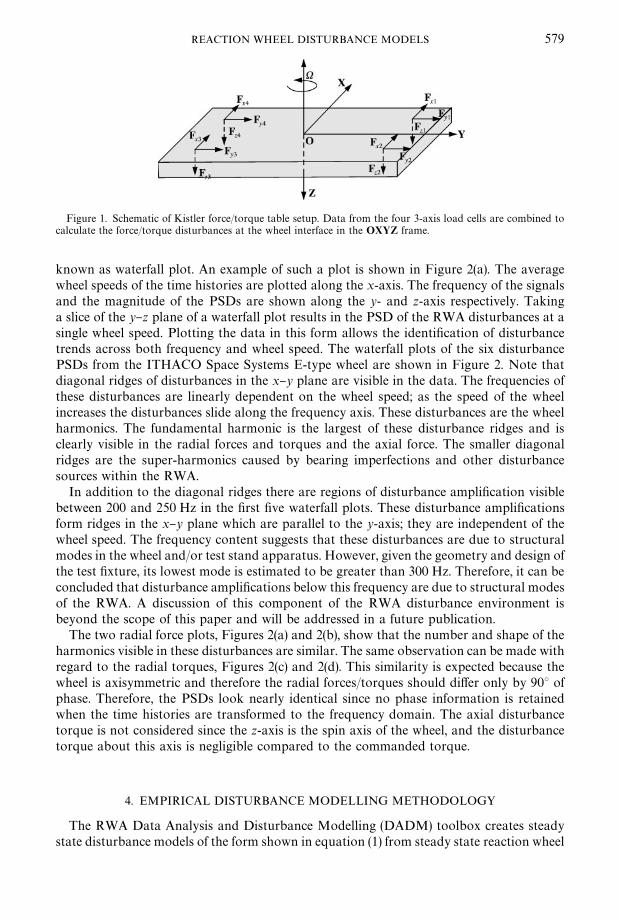
Figure 1. Schematic of Kistler force/torque table setup. Data from the four 3-axis load cells are combined tocalculate the force/torque disturbances at the wheel interface in the OXYZ frame.


known as waterfall plot. An example of such a plot is shown in Figure 2(a). The averagewheel speeds of the time histories are plotted along the x-axis. The frequency of the signalsand the magnitude of the PSDs are shown along the y- and z-axis respectively. Takinga slice of the y}z plane of a waterfall plot results in the PSD of the RWA disturbances at asingle wheel speed. Plotting the data in this form allows the identi"cation of disturbancetrends across both frequency and wheel speed. The waterfall plots of the six disturbancePSDs from the ITHACO Space Systems E-type wheel are shown in Figure 2. Note thatdiagonal ridges of disturbances in the x}y plane are visible in the data. The frequencies ofthese disturbances are linearly dependent on the wheel speed; as the speed of the wheelincreases the disturbances slide along the frequency axis. These disturbances are the wheelharmonics. The fundamental harmonic is the largest of these disturbance ridges and isclearly visible in the radial forces and torques and the axial force. The smaller diagonalridges are the super-harmonics caused by bearing imperfections and other disturbancesources within the RWA.

In addition to the diagonal ridges there are regions of disturbance ampli"cation visiblebetween 200 and 250 Hz in the "rst "ve waterfall plots. These disturbance ampli"cationsform ridges in the x}y plane which are parallel to the y-axis; they are independent of thewheel speed. The frequency content suggests that these disturbances are due to structuralmodes in the wheel and/or test stand apparatus. However, given the geometry and design ofthe test "xture, its lowest mode is estimated to be greater than 300 Hz. Therefore, it can beconcluded that disturbance ampli"cations below this frequency are due to structural modesof the RWA. A discussion of this component of the RWA disturbance environment isbeyond the scope of this paper and will be addressed in a future publication.

The two radial force plots, Figures 2(a) and 2(b), show that the number and shape of theharmonics visible in these disturbances are similar. The same observation can be made withregard to the radial torques, Figures 2(c) and 2(d). This similarity is expected because thewheel is axisymmetric and therefore the radial forces/torques should di!er only by 903 ofphase. Therefore, the PSDs look nearly identical since no phase information is retainedwhen the time histories are transformed to the frequency domain. The axial disturbancetorque is not considered since the z-axis is the spin axis of the wheel, and the disturbancetorque about this axis is negligible compared to the commanded torque.

4. EMPIRICAL DISTURBANCE MODELLING METHODOLOGY

The RWA Data Analysis and Disturbance Modelling (DADM) toolbox creates steadystate disturbance models of the form shown in equation (1) from steady state reaction wheel

Figure 2. RWA disturbance data*ITHACO E-type wheel: (a) radial force, x direction; (b) radial force,y direction; (c) radial torque, x direction; (d) radial torque, y direction; (e) axial force, z direction.


disturbance data. The analysis tools extract the model parameters, hi

and Ci, from

frequency domain data and generate plots for model validation. In this section, the dataanalysis and disturbance modelling process is discussed in detail using the development ofa radial force disturbance model from the ITHACO Space Systems E-type wheel F

xand

Fy

data as an example.

4.1. OVERVIEW

Typical test results from one wheel include data for "ve disturbances: three forces (Fx, F

y,

Fz) and two torques (¹

x, ¹

y). Assuming the z-axis is the spin axis of the wheel, the F

xand

Fydata are both radial force disturbances and are used in combination to create the radial

force disturbance model. The use of both data sets should result in better correlation


between the model and the data since the number of data points in the sample space isdoubled. Similarly, ¹

xand ¹

yare both radial torque data, and are used to create the radial

torque model. The axial force disturbance model is created from the Fz, or axial force, data.

The RWA DADM process requires that experimental data from a given wheel beprocessed and stored in "ve data sets, one for each of the relevant disturbances, that includeboth the PSDs, S, and amplitude spectra, A, of the measured disturbances, the wheel speedsat which the data were taken, X, a frequency vector corresponding to the frequency domaindata, f, and the upper frequency limit of good data, f

Lim. Both S and A are row vectors of

frequency domain data arranged such that the jth column corresponds to the PSD (oramplitude spectra) of the disturbance taken at the jth wheel speed, i.e., S"[S

12Sm]. The

upper frequency limit is determined by the frequency at which the data were sampled or thefrequency of the "rst test stand mode. It is only desirable to use data that are not corruptedby test "xture dynamics. Therefore, if a test stand mode exists below the Nyquist frequency,fLim

should be set at a frequency signi"cantly lower than the test stand resonance. Otherwise,fLim

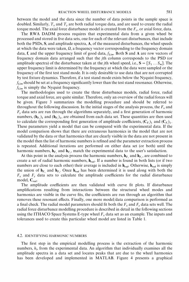
is simply the Nyquist frequency.The methodologies used to create the three disturbance models, radial force, radial

torque and axial force, are quite similar. Therefore, only an overview of the radial forces willbe given. Figure 3 summarizes the modelling procedure and should be referred tothroughout the following discussion. In the initial stages of the analysis process, the F

xand

Fydata sets are run through the algorithms separately, and a "rst generation of harmonic

numbers, (hFx

)1

and (hFy

)1, are obtained from each data set. These quantities are then used

to calculate the corresponding "rst generation of amplitude coe$cients, (CFx

)1

and (CFy)1.

These parameters yield a model that can be compared with the experimental data. If themodel comparison shows that there are extraneous harmonics in the model that are notvalidated by the data or that harmonics that are clearly visible in the data are not present inthe model then the list of harmonic numbers is re"ned and the parameter extraction processis repeated. Additional iterations are performed on either data set (or both) until theharmonic numbers, h

Fxand h

Fy, match the experimental data to the user's satisfaction.

At this point in the analysis process the harmonic numbers, hFx

and hFy

, are combined tocreate a set of radial harmonic numbers, h

rad. If a number is found in both lists (or if two

numbers are close to each other) their average is included in hrad

. Otherwise, hrad

is simplythe union of h

Fxand h

Fy. Once h

radhas been determined it is used along with both the

Fx

and Fy

data sets to calculate the amplitude coe$cients for the radial disturbancemodel, C

rad.

The amplitude coe$cients are then validated with curve "t plots. If disturbanceampli"cations resulting from interactions between the structural wheel modes andharmonics are visible in the curve "ts, the coe$cients are run through an algorithm thatremoves these resonant e!ects. Finally, one more model/data comparison is performed asa "nal check. The radial model parameters should "t both the F

xand F

ydata sets well. The

radial force disturbance modelling procedure is described in detail in the following sectionsusing the ITHACO Space Systems E-type wheel F

xdata set as an example. The inputs and

tolerances used to create this particular wheel model are listed in Table 1.

4.2. IDENTIFYING HARMONIC NUMBERS

The "rst step in the empirical modelling process is the extraction of the harmonicnumbers, h

i, from the experimental data. An algorithm that individually examines all the

amplitude spectra in a data set and locates peaks that are due to the wheel harmonicshas been developed and implemented in MATLAB. Figure 4 presents a graphical

Figure 3. RWA data analysis process for radial force disturbance.


representation of the harmonic number identi"cation algorithm and is referred tothroughout the following discussion.

First, the frequencies, f, are normalized by dividing the elements of the frequency vectorby each of the speeds (in revolutions per second, r.p.s.) in the wheel speed vector, X. Theresult is m vectors of non-dimensional frequency ratios (where m is the total number ofwheel speeds), f *

j, each corresponding to one wheel speed, X

j. Figure 5 demonstrates the

normalization using the ITHACO Space Systems E-type wheel Fx

data at X"2000

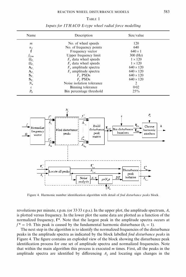
TABLE 1

Inputs for I¹HACO E-type wheel radial force modelling

Name Description Size/value

m No. of wheel speeds 120nf

No. of frequency points 640f Frequency vector 640]1

fLim

Upper frequency limit 300 (Hz)X

FxFx

data wheel speeds 1]120X

FyFydata wheel speeds 1]120

AFx

Fx

amplitude spectra 640]120A

FyFyamplitude spectra 640]120

SFx

Fx

PSDs 640]120SFy

FyPSDs 640]120

Np Noise isolation tolerance 2e Binning tolerance 0)02P0

Bin percentage threshold 25%

Figure 4. Harmonic number identi"cation algorithm with detail of ,nd disturbance peaks block.


revolutions per minute, r.p.m. (or 33)33 r.p.s.). In the upper plot, the amplitude spectrum, A,is plotted versus frequency. In the lower plot the same data are plotted as a function of thenormalized frequency, f *. Note that the largest peak in the amplitude spectra occurs atf *"1)0. This peak is caused by the fundamental harmonic disturbance (h

i"1).

The next step in the algorithm is to identify the normalized frequencies of the disturbancepeaks in the amplitude spectra as indicated by the block labelled ,nd disturbance peaks inFigure 4. The "gure contains an exploded view of the block showing the disturbance peakidenti"cation process for one set of amplitude spectra and normalized frequencies. Notethat within the main algorithm this process is executed m times. First, all the peaks in theamplitude spectra are identi"ed by di!erencing A

jand locating sign changes in the

Figure 5. Frequency normalization of ITHACO E-type wheel Fx

data (2000 r.p.m.): (a) amplitude spectrumversus frequency; (b) amplitude spectrum versus normalized frequency.


di!erenced data. The quantities f *jpeak

and Ajpeak

are the normalized peak frequencies andamplitudes respectively. For example, each peak identi"ed in ITHACO Space SystemsE-type wheel amplitude spectra A at X"2000 r.p.m. is shown in Figure 6(a) marked withan &&x''. Note that all of the peaks in the data are marked. It is highly unlikely that all of thesepeaks are a result of harmonic disturbances. Some may be due to noise or may be a result oftaking the FFT of the time history data. Therefore, a method was developed to discriminatebetween disturbance peaks and noise peaks.

Noise is isolated from the disturbance harmonics in the block labelled noise analysis. TheMATLAB histogram function is used to bin the elements of A

jpeakaccording to amplitude.

Assuming that the noise peaks are all of roughly the same amplitude and account forthe largest bin in the histogram allows a disturbance amplitude threshold, D¹, tobe determined. All spike amplitudes that fall in or below the largest histogram bin areconsidered noise. The remaining spikes are considered possible harmonic disturbances. SeeFigure 6(b) for an example. The disturbance amplitude threshold is then de"ned as

D¹"knoise

#Nppnoise, (3)

where knoise

and pnoise

are the mean and standard deviation of the spike amplitudesidenti"ed by the histogram. The parameter Np is a user-de"ned tolerance level. Its defaultvalue is 3, but can be adjusted according to the signal-to-noise ratio of the data. TheITHACO Space Systems E-type wheel data, for example, were sampled at a relatively highfrequency (3840 Hz) and for a long time. Therefore, a small frequency resolution and goodsignal-to-noise ratio were obtained, which allows the use of a lower noise isolationtolerance, Np"2.

All peaks with an amplitude below the disturbance amplitude threshold are not includedin the "nal vector of disturbance peaks. This part of the algorithm is represented in thediagram by the block labelled disturbance peak isolation. The "nal outputs of the ,nddisturbance peaks algorithm are a vector of normalized disturbance peak frequencies,

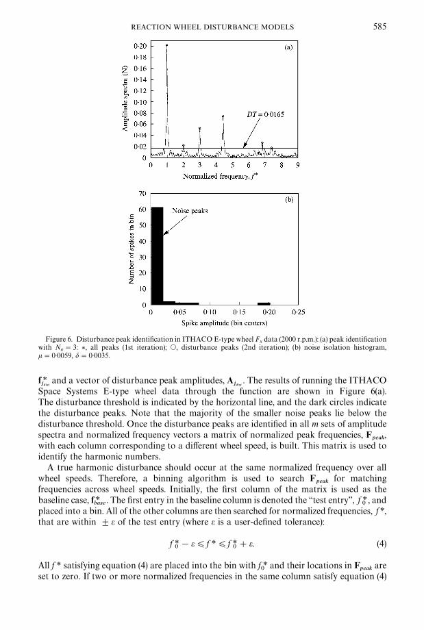
Figure 6. Disturbance peak identi"cation in ITHACO E-type wheel Fxdata (2000 r.p.m.): (a) peak identi"cation

with Np"3: *, all peaks (1st iteration); s, disturbance peaks (2nd iteration); (b) noise isolation histogram,k"0)0059, d"0)0035.


f *jdist

and a vector of disturbance peak amplitudes, Ajdist

. The results of running the ITHACOSpace Systems E-type wheel data through the function are shown in Figure 6(a).The disturbance threshold is indicated by the horizontal line, and the dark circles indicatethe disturbance peaks. Note that the majority of the smaller noise peaks lie below thedisturbance threshold. Once the disturbance peaks are identi"ed in all m sets of amplitudespectra and normalized frequency vectors a matrix of normalized peak frequencies, F

peak,

with each column corresponding to a di!erent wheel speed, is built. This matrix is used toidentify the harmonic numbers.

A true harmonic disturbance should occur at the same normalized frequency over allwheel speeds. Therefore, a binning algorithm is used to search F

peakfor matching

frequencies across wheel speeds. Initially, the "rst column of the matrix is used as thebaseline case, f *

base. The "rst entry in the baseline column is denoted the &&test entry'', f *

0, and

placed into a bin. All of the other columns are then searched for normalized frequencies, f *,that are within $e of the test entry (where e is a user-de"ned tolerance):

f *0!e)f *)f *

0#e. (4)

All f * satisfying equation (4) are placed into the bin with f *0

and their locations in Fpeak

areset to zero. If two or more normalized frequencies in the same column satisfy equation (4)


their average is placed in the bin, and both entries are set to zero. Averaging ensures thata possible harmonic will only be accounted for once at each wheel speed. When the entirematrix has been searched, the second element of f*

basebecomes the test entry and a new bin is

created. The process continues until all elements of f *base

have been considered. At this point,the second column becomes f *

baseand the search is repeated. The algorithm continues in this

manner until all non-zero elements of Fpeak

are binned. The results of the binning algorithmare a matrix of the binned normalized frequencies, F

bin(with the kth column corresponding

to the kth bin) and a second matrix containing the statistics for each bin, Fstat

. The "rst rowof F

statis the average, or center, of the bins, fM *

bink, and the second row contains the number of

elements in the bins, Nbink

.In the "nal block of Figure 4 the harmonic numbers are chosen from F

stat. A metric, P

k,

is de"ned as the percentage of possible wheel speeds in which a given normalized peakfrequency was found:

Pk"

Nbink

Npossk

100%, (5)

where Npossk

is the total possible number of elements in the kth bin. In general, Npossk

shouldbe equal to the number of wheel speeds in the data set. However, this assumption does notalways hold due to the frequency range of the data set. The value of f

Limmay limit the

number of wheel speeds in which a given normalized peak frequency is visible. For example,as mentioned earlier, the E Wheel is free of corruption by test stand dynamics in the range[0, 300] Hz. Any data above 300 Hz is not used in the modelling process. The normalizedfrequency 1)0 corresponds to 8)3 Hz when the wheel is spinning at 500 r.p.m. and to 56)7 Hzat 3400 r.p.m. Since both frequencies lie within the frequency range [0, 300] a disturbance atf *"1)0 can be observed at all wheel speeds. The normalized frequency 5)98, on the otherhand, corresponds to 49)8 Hz at 500 r.p.m. and 339 Hz at 3400 r.p.m. In this case, f * lieswithin the speci"ed frequency range for only a subset of the wheel speeds. The value ofN

posskis therefore not the same over all k bins.

The metric Pkcan be considered a measure of the strength of a disturbance across wheel

speeds, and is used to identify wheel harmonics from the list of bin centers, fM *bink

in Fstat

. IfPkis greater than a user-de"ned threshold, P

0, then fM *

binkis de"ned to be a harmonic number

and placed into a new vector, h. The outputs of the harmonic number identi"cationalgorithm are this vector of harmonic numbers, h, and the matrix of normalized disturbancepeak frequencies, F

peak. Both outputs are necessary for the next step of the modelling

process.To create a complete wheel model, the harmonic number identi"cation process described

above is performed on the three force and two torque disturbances. Then, the radial forceand radial torque model harmonic numbers, h

radand h

tor, are determined by comparing and

combining the harmonic numbers extracted from the Fxand F

ydata and the ¹

xand ¹

ydata

respectively. The axial force harmonic numbers, haxi

, are the harmonic numbers extractedfrom the F

zdata.

4.3. CALCULATING AMPLITUDE COEFFICIENTS

The next step in the empirical modelling process is the extraction of the amplitudecoe$cients, C

i, from the experimental data. Figure 7 presents a graphical representation of

the algorithm used to calculate the amplitude coe$cients given a steady state RWA dataset, the harmonic numbers, h, and matrix of normalized disturbance peak frequencies, F

peak.

Figure 7. Amplitude coe$cient calculation algorithm.


The block diagram details the process for one harmonic and its corresponding amplitudecoe$cient. In practice, the algorithm is repeated for each harmonic in the model.

Least-squares approximation methods are used to calculate the amplitude coe$cients forthe HST RWA disturbance model [14]. The magnitude of the disturbance force (or torque)is assumed to be related to the wheel speed as

dIij"K

iX2

j, (6)

where dIij

is the expected disturbance force (or torque) at the frequency corresponding to theith harmonic at the jth wheel speed and K

iis a constant. The error between the actual

disturbance and the expected disturbance at the ith harmonic and the jth wheel speed, eij

isthen

eij"d

ij!K

iX2

j, (7)

where dij

is the experimentally measured disturbance force at the ith harmonic and jth wheelspeed. The amplitude coe$cient, C

i, is de"ned as the value of K

ithat minimizes this error.

An expression for Ciis obtained by squaring equation (7), summing over the wheel speeds

and solving for the Kithat minimizes the squared error, e2

ij:

Ci"

+mj/1

dijX2

j+m

j/1X4

j

. (8)

Recall that during the initial stages of the radial force/torque modelling procedure thecoe$cients are calculated from a single data set, but the "nal model coe$cients arecalculated using two data sets (see Figure 3). The RWA DADM algorithm uses equation (8)to compute the coe$cients for either the single or double data set case as shown in Figure 7.In the following discussion, multiple data set extraction of radial force amplitudecoe$cients from the ITHACO Space Systems E-type wheel F

xand F

ydata will be used as an

example.The "rst block in Figure 7 represents the normalization of the frequency vector, f. The

resulting non-dimensional frequency vectors, Mf *1 2f *

mN are used along with A, F

peak, X and

h to determine the disturbance forces, dij, at each harmonic number over all wheel speeds. It

is important to note that a disturbance at the ith harmonic may not be visible in all of theamplitude spectra in the data set. A disturbance peak can be undetectable for one of tworeasons. If the frequency corresponding to h

ifor a given wheel speed, X

j, is not within the

frequency range of good data, [0, fLim

], the disturbance amplitude at this frequency may be


corrupted and is not included in the calculation of the amplitude coe$cient. In addition, notall disturbances that fall within the frequency range are visible at all wheel speeds. Forexample, disturbances are often more di$cult to identify in data taken at low wheel speedsdue to a low signal-to-noise ratio. Therefore, the data must meet certain peak detectionconditions to be included in the calculation of C

i.

Recall that both the matrix of amplitude spectra, A, and Fpeak

contain m columns, eachcorresponding to one wheel speed. De"ning the quantity D

jwhich contains the amplitude

spectra, wheel speed, normalized frequency vector, normalized peak locations, and upperfrequency limit of good data associated with one wheel speed, D

j(A

j, f *

j, F

peakj, X

j, f

Lim)

allows the peak detection conditions to be written as

Dj"M0(h

iX

j)f

LimNWM f *3F

peakjDh

i!e)f *)h

i#eN. (9)

The "rst condition in equation (9) ensures that the frequency corresponding to theharmonic for X

jis within the frequency range of good data. The second condition uses the

matrix of detected normalized peak frequencies, Fpeak

, obtained from the harmonic numberidenti"cation algorithm to ensure that a disturbance peak at f *"h

iis detectable in the

amplitude spectra.The extraction of disturbance amplitudes for use in the amplitude coe$cient calculation

is done one wheel speed at a time. The amplitude spectrum provides an estimation of thesignal amplitude over frequency. Therefore, if D

jsatis"es both of the above conditions the

magnitude of the disturbance force/torque at the frequency corresponding to the ithharmonic is simply the value of A

jat the normalized frequency f *"h

i. The disturbance

magnitude is assigned to dij, and the wheel speed is assigned to XI

ij. However, if one or both

of the conditions are not satis"ed, the data for that wheel speed is not included in thecalculation and both d

ijand XI

ijare set to zero. This process is continued for all wheel

speeds, until two vectors of length m, one of disturbance amplitudes, Di, and one of

corresponding wheel speeds, XIi, are created. In general, XI

iwould be equal to the input

vector X, but since all of the wheel speeds may not be included in the amplitude coe$cientcalculation for a given harmonic due to lack of disturbance peak visibility, each C

iis

computed using a distinct subset of wheel speeds, XIi. The vectors D

iand XI

iare manipulated

and summed as shown in equation (8) to obtain Ci.

Curve-"t plots are useful for both removing harmonics from the model and assessing thequality of the "t between the data and the disturbance force predicted by C

i. The plots for

the 1)0 and 4)42 harmonics of the ITHACO Space Systems E-type wheel data (Fxand F

y) are

shown in Figure 8. The circles represent the disturbance amplitudes of the experimentaldata over the di!erent wheel speeds, D

i. Note that some of the circles lie on the x-axis. These

points are from wheel speeds which did not meet the conditions in equation (9). The solidline is the curve generated using the calculated C

iand equation (6).

Notice in the curve "t plot for h1"1)0 that the data points are not distributed evenly

across wheel speeds, but are clustered at high wheel speeds. Recall that when the vibrationtests were conducted, full torque was applied to the wheel and it was allowed to spin upuntil it reached saturation around 2300 r.p.m. As a result, a large portion of the data wastaken while the wheel was saturated at its maximum speed. Therefore, when the data wereprocessed into quasi-steady state data sets, the highest wheel speed was representedmultiple times in the wheel speed vector and frequency domain data matrices. Thealgorithm used to calculate the amplitude coe$cients ensures that the uneven wheel speeddistribution does not result in an unequal weighting of the data points when the amplitudecoe$cient is calculated. If a data point from a given wheel speed is included more than oncein the vector D

i, the wheel speed is also included an equal number of times in XI

i.

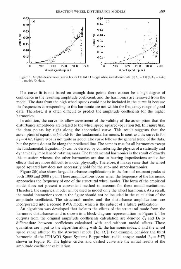
Figure 8. Amplitude coe$cient curve "ts for ITHACO E-type wheel radial force data: (a) h1"1)0; (b) h

5"4)42;

**, model; s, data.


If a curve "t is not based on enough data points there cannot be a high degree ofcon"dence in the resulting amplitude coe$cient, and the harmonics are removed from themodel. The data from the high wheel speeds could not be included in the curve "t becausethe frequencies corresponding to this harmonic are not within the frequency range of gooddata. Therefore, it is often di$cult to predict the amplitude coe$cients for the higherharmonics.

In addition, the curve "ts allow assessment of the validity of the assumption that thedisturbance amplitudes are related to the wheel speed squared (equation (6)). In Figure 8(a),the data points lay right along the theoretical curve. This result suggests that theassumption of equation (6) holds for the fundamental harmonic. In contrast, the curve "t forh5"4)42, Figure 8(b), is not quite as good. The curve follows the general trend of the data,

but the points do not lie along the predicted line. The same is true for all harmonics exceptthe fundamental. Equation (6) can be derived by considering the physics of a statically anddynamically imbalanced rotating mass. The fundamental harmonics is the result of exactlythis situation whereas the other harmonics are due to bearing imperfections and othere!ects that are more di$cult to model physically. Therefore, it makes sense that the wheelspeed squared law does not necessarily hold for the sub- and super-harmonics.

Figure 8(b) also shows large disturbance ampli"cations in the form of resonant peaks atboth 1000 and 2000 r.p.m. These ampli"cations occur when the frequency of the harmonicapproaches the frequency of one of the structural wheel modes. The form of the empiricalmodel does not present a convenient method to account for these modal excitations.Therefore, the empirical model will be used to model only the wheel harmonics. As a result,the modal interactions seen in the "gure should not be included in the calculation of theamplitude coe$cient. The structural modes and the disturbance ampli"cations areincorporated into a second RWA model which is the subject of a future publication.

An algorithm was developed that isolates the e!ects of the structural mode from theharmonic disturbances and is shown in a block-diagram representation in Figure 9. Theoutputs from the original amplitude coe$cients calculation are denoted CM

iand D1

ito

di!erentiate between coe$cients calculated with and without modal e!ects. Thesequantities are input to the algorithm along with X, the harmonic index, i, and the wheelspeed range a!ected by the structural mode, [X

l, X

u]. For example, consider the third

harmonic of the ITHACO Space Systems E-type wheel radial torque model (h7"5)57)

shown in Figure 10. The lighter circles and dashed curve are the initial results of theamplitude coe$cient calculation.

Figure 9. Structural mode isolation algorithm.

Figure 10. E!ects of internal wheel modes on amplitude coe$cient curve "t; h7"5)57 (ITHACO E-type wheel

radial force): s, with modal e!ects, C7"1)73]10~8; x, w/o modal e!ects, C

7"0)69]10~8.


Note that there is a large increase in force amplitude in the data around 2300 r.p.m. Theresonant e!ect of the structural mode is removed from the amplitude coe$cient calculationby removing the data points associated with speeds in the a!ected range from D1

i. Then,

a new disturbance magnitude vector, Di, and corresponding wheel speed vector, XI

iare

created and used to calculate the corrected amplitude coe$cient, Ci.

The resulting curve "t without the modal e!ects included is also shown in Figure 10. Thedark x's and the solid curve correspond to D

7and C

7and do not include the resonance

points, while the lighter circles and dashed curve correspond to the original coe$cientcalculation based on all points, D1

7and C1

7. Note that including data with the resonance

behavior causes an over-estimation of the disturbance force over all wheel speeds (dashedcurve). When the resonant data are removed from the coe$cient calculation (solid curve)the amplitude coe$cient is decreased by 60% and there is a much better "t between thetheoretical curve and the data between 1500 and 2000 r.p.m.

Seven harmonics have been identi"ed for the ITHACO Space Systems E-type wheelradial force disturbance model with the analysis toolbox. A harmonic at h

i"5)00 and those

greater than 5)57 are eliminated from the model due to low-con"dence amplitude coe$cientcurve "ts. In most of these cases, the only signi"cant peaks are a result of disturbance

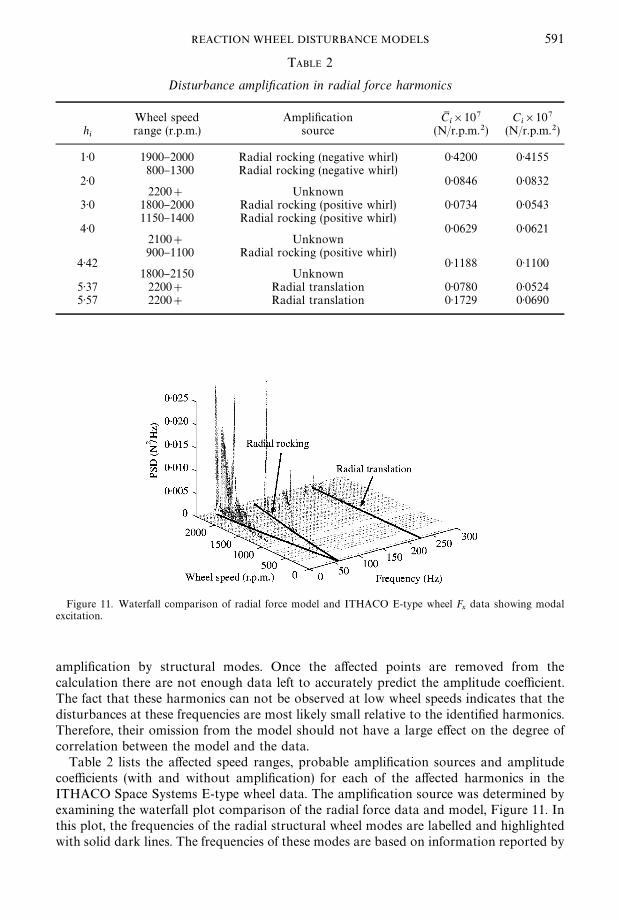
TABLE 2

Disturbance ampli,cation in radial force harmonics

Wheel speed Ampli"cation CMi]107 C

i]107

hi

range (r.p.m.) source (N/r.p.m.2) (N/r.p.m.2)

1)0 1900}2000 Radial rocking (negative whirl) 0)4200 0)4155800}1300 Radial rocking (negative whirl)

2)0 0)0846 0)08322200# Unknown

3)0 1800}2000 Radial rocking (positive whirl) 0)0734 0)05431150}1400 Radial rocking (positive whirl)

4)0 0)0629 0)06212100# Unknown900}1100 Radial rocking (positive whirl)

4)42 0)1188 0)11001800}2150 Unknown

5)37 2200# Radial translation 0)0780 0)05245)57 2200# Radial translation 0)1729 0)0690

Figure 11. Waterfall comparison of radial force model and ITHACO E-type wheel Fx

data showing modalexcitation.


ampli"cation by structural modes. Once the a!ected points are removed from thecalculation there are not enough data left to accurately predict the amplitude coe$cient.The fact that these harmonics can not be observed at low wheel speeds indicates that thedisturbances at these frequencies are most likely small relative to the identi"ed harmonics.Therefore, their omission from the model should not have a large e!ect on the degree ofcorrelation between the model and the data.

Table 2 lists the a!ected speed ranges, probable ampli"cation sources and amplitudecoe$cients (with and without ampli"cation) for each of the a!ected harmonics in theITHACO Space Systems E-type wheel data. The ampli"cation source was determined byexamining the waterfall plot comparison of the radial force data and model, Figure 11. Inthis plot, the frequencies of the radial structural wheel modes are labelled and highlightedwith solid dark lines. The frequencies of these modes are based on information reported by

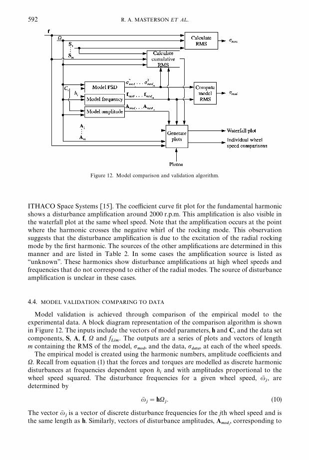
Figure 12. Model comparison and validation algorithm.


ITHACO Space Systems [15]. The coe$cient curve "t plot for the fundamental harmonicshows a disturbance ampli"cation around 2000 r.p.m. This ampli"cation is also visible inthe waterfall plot at the same wheel speed. Note that the ampli"cation occurs at the pointwhere the harmonic crosses the negative whirl of the rocking mode. This observationsuggests that the disturbance ampli"cation is due to the excitation of the radial rockingmode by the "rst harmonic. The sources of the other ampli"cations are determined in thismanner and are listed in Table 2. In some cases the ampli"cation source is listed as&&unknown''. These harmonics show disturbance ampli"cations at high wheel speeds andfrequencies that do not correspond to either of the radial modes. The source of disturbanceampli"cation is unclear in these cases.

4.4. MODEL VALIDATION: COMPARING TO DATA

Model validation is achieved through comparison of the empirical model to theexperimental data. A block diagram representation of the comparison algorithm is shownin Figure 12. The inputs include the vectors of model parameters, h and C, and the data setcomponents, S, A, f, X and f

Lim. The outputs are a series of plots and vectors of length

m containing the RMS of the model, pmod

, and the data, pdata

, at each of the wheel speeds.The empirical model is created using the harmonic numbers, amplitude coe$cients and

X. Recall from equation (1) that the forces and torques are modelled as discrete harmonicdisturbances at frequencies dependent upon h

iand with amplitudes proportional to the

wheel speed squared. The disturbance frequencies for a given wheel speed, uNj, are

determined by

u6j"hX

j. (10)

The vector u6jis a vector of discrete disturbance frequencies for the jth wheel speed and is

the same length as h. Similarly, vectors of disturbance amplitudes, Amodj

, corresponding to


u6j

are created based on the assumption that the disturbance amplitude from the ithharmonic at the jth wheel speed is

Amodij

"CiX2

j. (11)

The matrices Amod

and u6 , which are analogous to the experimental quantities A and f, areused to generate model/data comparison plots.

In addition, the PSD of the model, Smodj

, is calculated for comparison to the experimentaldata. An expression for the model PSD as a function of frequency and wheel speed isderived from the de"nition of the autocorrelation, R

X(q):

RX(q)"R

X(t, t#q)"E[X(t)X (t#q)]. (12)

Substituting m(t) (equation (1)) for X(t) in equation (12) and assuming that aiis a random

variable uniformly distributed between 0 and 2n and that ai

and aj

are statisticallyindependent, the expression for the autocorrelation of the empirical model becomes

Rm(q)"

n+i/1

C2iX4

j2

cos (Xjhiq). (13)

The mean square of a random process is equal to its autocorrelation evaluated at q"0.Therefore, assuming that m(t) is both stationary and zero mean, the variance of theempirical model is

p2modj

"Rm(0)"

n+i/1

C2iX4

j2

. (14)

Equations (13) and (14) are then used to derive the spectral density function of theempirical model. The autocorrelation function of a single harmonic process and itscorresponding spectral density are given in reference [20] as

RX (q)"p2x cos (u0q), (15)

Sx(u)"p2x C1

2d(u#u

0)#

1

2d (u!u

0)D . (16)

Substituting equation (14) into equation (12) and setting hiX

j"u

0results in an

autocorrelation of the same form as that in equation (15). Therefore, the PSD of theempirical model is of the same from as that in equation (16). After making the necessarysubstitutions the one-sided PSD of the empirical model, S

modj(u), is

Smodj

(u)"n+i/1

C2iX4

j2

d (u!u6j). (17)

Note that the empirical model PSD consists of a series of discrete impulses occurring atfrequencies, u6

j, with amplitudes equal to the variances of the harmonics, p2

modij. The vectors

[p2mod12

p2modm

], which are outputs of the &&model PSD'' block in Figure 12, consist of thePSD amplitudes for the discrete harmonics at all m wheel speeds. The matrix of thesevectors, p2

modis analogous to S and is used for model/data comparison.

The RMS values of the model and data are calculated for each wheel speed. The areaunder the PSD of a random process is equal to the mean square. Therefore, the data RMSfor a given wheel speed, p

dataj, is simply the square root of the area under the PSD, S

j.

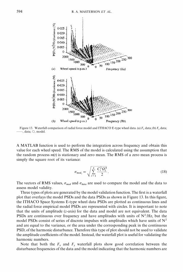
Figure 13. Waterfall comparison of radial force model and ITHACO E-type wheel data. (a) Fxdata; (b) F

ydata;

**, data; s, model.


A MATLAB function is used to perform the integration across frequency and obtain thisvalue for each wheel speed. The RMS of the model is calculated using the assumption thatthe random process m(t) is stationary and zero mean. The RMS of a zero mean process issimply the square root of its variance:

pmodj

"Sn+i/1

C2iX4

j2

. (18)

The vectors of RMS values, pmod

and pdata

are used to compare the model and the data toassess model validity.

Three types of plots are generated by the model validation function. The "rst is a waterfallplot that overlays the model PSDs and the data PSDs as shown in Figure 13. In this "gure,the ITHACO Space Systems E-type wheel data PSDs are plotted as continuous lines andthe radial force empirical model PSDs are represented with circles. It is important to notethat the units of amplitude (z-axis) for the data and model are not equivalent. The dataPSDs are continuous over frequency and have amplitudes with units of N2/Hz, but themodel PSDs consist of series of discrete impulses with amplitudes which have units of N2

and are equal to the variance, or the area under the corresponding peak in the continuousPSD, of the harmonic disturbance. Therefore this type of plot should not be used to validatethe amplitude coe$cients of the model. Instead, the waterfall plot is useful for validating theharmonic numbers.

Note that both the Fx

and Fy

waterfall plots show good correlation between thedisturbance frequencies of the data and the model indicating that the harmonic numbers are

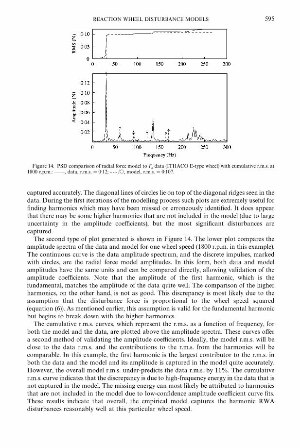
Figure 14. PSD comparison of radial force model to Fxdata (ITHACO E-type wheel) with cumulative r.m.s. at

1800 r.p.m.: **, data, r.m.s."0)12; - - - /s, model, r.m.s."0)107.


captured accurately. The diagonal lines of circles lie on top of the diagonal ridges seen in thedata. During the "rst iterations of the modelling process such plots are extremely useful for"nding harmonics which may have been missed or erroneously identi"ed. It does appearthat there may be some higher harmonics that are not included in the model (due to largeuncertainty in the amplitude coe$cients), but the most signi"cant disturbances arecaptured.

The second type of plot generated is shown in Figure 14. The lower plot compares theamplitude spectra of the data and model for one wheel speed (1800 r.p.m. in this example).The continuous curve is the data amplitude spectrum, and the discrete impulses, markedwith circles, are the radial force model amplitudes. In this form, both data and modelamplitudes have the same units and can be compared directly, allowing validation of theamplitude coe$cients. Note that the amplitude of the "rst harmonic, which is thefundamental, matches the amplitude of the data quite well. The comparison of the higherharmonics, on the other hand, is not as good. This discrepancy is most likely due to theassumption that the disturbance force is proportional to the wheel speed squared(equation (6)). As mentioned earlier, this assumption is valid for the fundamental harmonicbut begins to break down with the higher harmonics.

The cumulative r.m.s. curves, which represent the r.m.s. as a function of frequency, forboth the model and the data, are plotted above the amplitude spectra. These curves o!era second method of validating the amplitude coe$cients. Ideally, the model r.m.s. will beclose to the data r.m.s. and the contributions to the r.m.s. from the harmonics will becomparable. In this example, the "rst harmonic is the largest contributor to the r.m.s. inboth the data and the model and its amplitude is captured in the model quite accurately.However, the overall model r.m.s. under-predicts the data r.m.s. by 11%. The cumulativer.m.s. curve indicates that the discrepancy is due to high-frequency energy in the data that isnot captured in the model. The missing energy can most likely be attributed to harmonicsthat are not included in the model due to low-con"dence amplitude coe$cient curve "ts.These results indicate that overall, the empirical model captures the harmonic RWAdisturbances reasonably well at this particular wheel speed.

Figure 15. r.m.s. comparison of empirical model and ITHACO E-type wheel data: radial forces: #, Fxdata; *,

Fydata; s, radial model.


The third type of model/data comparison used for model validation is shown in Figure15. In this plot, the r.m.s. values of the data and the model are plotted as a function of wheelspeed. In e!ect, the plot is simply an integration of the waterfall plot across frequency. Thesolid curves, marked with &&#'' and &&*'' are the r.m.s. values for the F

xand F

ydata,

respectively, and are quite similar, as is expected. The "gure shows that over most wheelspeeds the model under-predicts the data slightly, but not by a signi"cant amount.However, there is a large amount of energy in the data between 1800 and 2000 r.p.m. that isnot captured in the model. Referring to Table 2, note that both the "rst and third harmonicsexcite the structural rocking mode of the wheel in this speed range. Therefore, a discrepancybetween the data and the model in this range exists because the empirical model does notaccount for the structural modes of the wheel. The smaller peaks in the data r.m.s. between800 and 1200 r.p.m. can also be attributed to the structural wheel modes by similarreasoning.

5. CONCLUSIONS

A set of MATLAB functions has been created to extend the HST model and facilitate theempirical modelling process. The toolbox extracts empirical model parameters from steadystate RWA vibration data allowing the creation of an empirical disturbance model for anygiven RWA assuming that the wheel disturbances are a series of harmonics at discretefrequencies with amplitudes proportional to the wheel speed squared. The toolbox takesadvantage of data analysis techniques to allow the user to quickly create disturbancemodels for a number of RWA. These models can be used in a disturbance analysisframework to conduct trade studies on di!erent types of RWA, enabling the engineer toselect the wheel that is best suited for a given application.

Steady state vibration data from an ITHACO Space Systems E-type wheel were used asan example to illustrate the capability of the toolbox and to validate the model. Waterfall


plots and r.m.s. comparison plots were used to compare the model to the data allowing anassessment of the accuracy of the empirical model and the performance of the toolbox. Thedata correlation for the ITHACO Space Systems E-type wheel model is quite good overmost wheel speeds. The waterfall plot comparison indicates that the disturbance frequenciesare identi"ed accurately; the harmonic numbers in the model are also visible in the data.The amplitudes of the disturbances also seem reasonable since the r.m.s. values of the dataand model are close over the wheel speed ranges that do not include disturbanceampli"cations. For example, at 1800 r.p.m. the model r.m.s. is 0)107 and the data r.m.s. is0)12, an error of only 11%. Over all wheel speeds between 56 and 2400 r.p.m. the modelunder-predicts the data by an average error of 20%; the model disturbance amplitudes arewithin a factor of two of the data.

The under-prediction of the ITHACO Space Systems E-type wheel model is mostpronounced over discrete ranges of speeds that show signi"cant disturbance ampli"cationsin the data that are not matched by the model. These peaks in r.m.s. result when thestructural wheel modes are excited by the harmonic disturbances. Such a peak is visible inthe E Wheel r.m.s. plot at about 1900 r.p.m. The data r.m.s. at this wheel speed is 0)52N andthe model r.m.s. is only 0)117N. At this wheel speed the model under-predicts the data by77%. Such large discrepancies exist in the a!ected wheel speed ranges because the internalwheel #exibility is not captured in the empirical model. The overall r.m.s. error of 20% isdriven by these disturbance ampli"cations.

It is concluded that although the empirical model captures the wheel harmonics andidenti"es the disturbance frequencies well, it alone is not an accurate RWA disturbancemodel. Excitation of the structural wheel modes by the harmonics can cause largedisturbance ampli"cations that must be included in the model to accurately predict thee!ects of the disturbances on the spacecraft during operation. An analytical disturbancemodel has been developed to take the resonant e!ects into account and is the subject ofa future publication. It is a combination of the analytical and empirical models that does thebest job of capturing the RWA disturbance environment. Therefore, the empirical modeland parameter extraction methodology is a major component of an accurate RWAdisturbance model.

The MATLAB toolbox described in this paper can be applied to steady statemicro-vibration data from any reaction wheel to provide the harmonic numbers andamplitude coe$cients that are necessary components of the complete disturbance model fora given RWA. In this way, the toolbox generalizes the empirical modelling process forapplication to any mission in which structural dynamics and control play a key role inmeeting performance requirements.

ACKNOWLEDGMENTS

The ITHACO E-type wheel data discussed in this paper were obtained thanks to GaryMosier (Goddard Space Flight Center), Gary Brown (Goddard Space Flight Center) andMr. Oliver DeWeck (MIT Space Systems Laboratory). Dr. Homero Gutierrez alsocontributed through his previous work, technical suggestions and support.

The work described in this paper was conducted in part at the Massachusetts Instituteof Technology under a contract with the Jet Propulsion Laboratory, CaliforniaInstitute of Technology and in part at the Jet Propulsion Laboratory, California Institute ofTechnology, under a contract with the National Aeronautics and Space Administration.Additional support for the work was provided by TRW Space & Electronics Groupthrough a graduate student fellowship.


REFERENCES

1. R. S. DANNER and S. UNWIN (editors) 1999 Space Interferometry Mission: ¹aking the Measure ofthe ;niverse. Pasadena: Jet Propulsion Laboratory, California Institute of Technology.

2. R. A. LASKIN 1995 in American Institute of Aeronautics and Astronautics Aerospace SciencesMeeting and Exhibit, AIAA 95-0825. Technology for space optical interferometry.

3. R. A. LASKIN and M. SAN MARTIN 1989 in Proceedings of AAS/AIAA Astrodynamics SpecialistConference, AAS 89-424, 369}395. Control/structure system design of a spaceborne opticalinterferometer.

4. O. DE WECK, D. MILLER and H. GUTIERREZ 1998 in Proceedings of the 34th ¸iege InternationalAstrophysics Colloquium, 269}273. Noordwijk, Netherlands: European Space Agency. Structuraldynamics and controls for NGST*a preliminary study.

5. B. BIALKE 1998 in Proceedings of the 21st Annual AAS Rocky Mountain Guidance and ControlConference, AAS paper 98-0634, 483}496. San Diego: Univelt, Inc. High "delity mathematicalmodeling of reaction wheel performance.

6. T. MARSHALL, T. GUNDERMAN and F. MOBLEY 1991 in Proceedings of the Annual RockyMountain Guidance and Control Conference, AAS paper 91-038, 119}138. San Diego: Univelt, Inc.Reaction wheel control of the MSX satellite.

7. L. P. DAVIS, J. F. WILSON, R. E. JEWELL and J. J. RODEN 1986. Hubble space telescope reactionwheel assembly vibration isolation system.

8. T. FUKUDA, H. HOSOKAI and N. YAJIMA 1986 Bulletin of the JSME 29, 3121}3125. Flexibilitycontrol of solar battery arrays (3rd Report, vibration and attitude control with consideration ofthe dynamics of a reaction wheel as an actuator).

9. S. SABNIS, F. SCHMITT and L. SMITH 1976 Sperry Flight Systems, Jet Propulsion ¸aboratoryNASA ¹echnical Report N76-27336. Magnetic bearing reaction wheel.

10. J. A. BOSGRA and J. J. M. PRINS 1982 in Automatic Control in Space (9th Symposium), 449}458.Testing and investigation of reaction wheels.

11. L. P. DAVIS, D. CUNNINGHAM and J. HARRELL 1994 in AIAA/ASME/ASCE/AHS/ASCStructures, Structural Dynamics, and Materials Conference, AIAA paper 94-1651, 2655}2665.Advanced 1)5 Hz passive viscous isolation system.

12. Sperry Flight Systems 1976 NASA/Marshall Space Flight Center, NASA ¹echnical ReportN76-18213. An evaluation of reaction wheel emitted vibrations for large space telescope.

13. K. J. PENDERGAST and C. J. CHAUWECKER 1998 in SPIE Conference on Space ¹elescopes andInstruments, Vol. 3356 (Part 2 of 2), 1078}1094. Use of a passive reaction wheel jitter isolationsystem to meet the advanced X-ray astrophysics facility imaging performance requirements.

14. M. D. HASHA 1986 Space ¹elescope Program Engineering Memo SSS 218. Reaction wheelmechanical noise variations.

15. B. BIALKE 1997 in 20th Annual American Aeronautical Society Guidance and Control Conference,AAS paper 97-038. A compilation of reaction wheel induced spacecraft disturbances.

16. B. LI, G. GODDU and M. CHOW 1998 in Proceedings of the American Control of Conference,2032}2036. Detection of common motor bearing faults using frequency-domain vibration signalsand a neural network based approach.

17. G. W. NEAT, J. W. MELODY and B. J. LURIE 1998 IEEE ¹ransactions on Control Systems¹echnology 6, 689}700. Vibration attenuation approach for spaceborne optical interferometers.

18. H. L. GUTIERREZ 1999 Ph.D. ¹hesis, Massachusetts Institute of ¹echnology. Performanceassessment and enhancement of precision controlled structures during conceptual design.

19. O. DE WECK 1999 Master1s ¹hesis, Massachusetts Institute of ¹echnology. Integrated modelingand dynamics simulation for the next generation space telescope.

20. P. H. WIRSCHING, T. L. PAEZ and H. OORTIZ 1995 Random <ibrations: ¹heory and Practice.New York: John Wiley & Sons Inc.

development and validation of reaction wheel disturbance models

Documents