developing a line balancing tool for reconfigurable
TRANSCRIPT

Developing a line balancing tool for reconfigurable manufacturing systems
PAPER WITHIN: Production systems AUTHORS: Mohamed Elnourani Abdelmageed & Filip Skärin JÖNKÖPING: June 2021
A tool to support investment decisions
Postadress: Besöksadress: Telefon: Box 1026 Gjuterigatan 5 036-10 10 00 (vx) 551 11 Jönköping
This final thesis has been carried out at School of Engineering in Jönköping within the
subject area production systems. The work is a part of the Master of Science program
Production Development and Management. The authors take full responsibility for the
opinions, findings and conclusions presented.
Examiner: Carin Rösiö
Supervisor: Gary Linnéusson
Scope: 30 credits (second cycle)
Date: 2021-06-03
Abstract
I
Abstract
Purpose This thesis aims to developing a decision-making tool which fits in
a reconfigurable manufacturing system (RMS) milieu used to
identify whether to introduce and produce a new product into an
already existing assembly line or to invest in a new assembly line.
To fulfil the purpose, four research questions were developed.
Method Literature studies were performed in order to create a theoretical
foundation for the thesis to stand upon, hence enabling the possibility
to answer the research questions. The literature studies were
structured to focus on selected topics, including reconfigurable
manufacturing systems, line balancing, and assembly line
investment costs. To answer the third research question, which
involved creating a decision-making tool, a single-case study was
carried out. The company chosen was within the automotive
industry. Data was collected through interviews, document studies
and a focus group.
Findings
& Analysis
An investigation regarding which line balancing solving-techniques
suit RMS and which assembly line investment costs are critical when
introducing new products has been made. The outputs from these
investigations set the foundation for developing a decision-making
tool which enables fact-based decisions. To test the decision-making
tool’s compatibility with reconfigurable manufacturing systems, an
evaluation against established characteristics was performed. The
evaluation identified two reconfigurable manufacturing system
characteristic as having a direct correlation to the decision-making
tool. These characteristics regarded scalability and convertibility.
Conclusions
The industrial contribution of the thesis was a decision-making tool
that enables fact-based decisions regarding whether to introduce a
new product into an already existing assembly line or invest in a new
assembly line. The academic contribution involved that the
procedure for evaluating the tool was recognized as also being
suitable for testing the reconfigurable correlation with other
production development tools. Another contribution regards
bridging the knowledge gaps of the classifications in line balancing-
solving techniques and assembly line investment costs.
Delimitations One of the delimitations in the thesis involved solely focusing on
developing and analysing a decision-making tool from an RMS
perspective. Hence, other production systems were not in focus.
Also, the thesis only covered the development of a decision-making
tool for straight assembly lines, not U-shaped lines.
Keywords Reconfigurable manufacturing systems, Line balancing, Assembly
lines, Case study, Decision-making tool
Acknowledgment
II
Acknowledgment
We would like to grasp the opportunity to show our gratitude to the people who have
supported and helped us during this master thesis. First of all, we would like to thank
the case company for enabling us to be a part of their project and for providing valuable
data and information. Also, we would like to send a special thanks to our contact person
and supervisor Tobias, for all your help and support.
We would also like to address our greatest appreciation for our supervisor Gary
Linnéusson at School of Engineering in Jönköping. Especially for your fantastic ability
to constantly provide us with new ideas and suggestions. We have learned a great deal
from you.
Lastly, we would also like to thank Simon Boldt for introducing the thesis proposal to
us, ensuring we would get a very valuable head start in writing the thesis during these
uncertain times.
Contents
III
Table of Contents
1 Introduction ...................................................................................................................... 1 1.1 Background ................................................................................................................ 1 1.2 Problem description ................................................................................................... 2 1.3 Purpose & research questions ................................................................................... 3 1.4 Delimitations .............................................................................................................. 4 1.5 Thesis outline .............................................................................................................. 4
2 Theoretical Framework ................................................................................................... 6 2.1 Reconfigurable manufacturing systems...................................................................... 6
2.1.1 RMS classification .................................................................................................... 7 2.1.2 RMS characteristics ................................................................................................... 7 2.1.3 RMS characteristics and improvement levels ......................................................... 10
2.2 Single-, mixed- & multi-model assembly lines ......................................................... 11 2.3 Line balancing problems .......................................................................................... 12 2.4 Decision-making tools in line balancing .................................................................. 13 2.5 Line balancing models and computation.................................................................. 14 2.6 Key performance indicators in line balancing ......................................................... 15 2.7 Assembly line investment costs ................................................................................. 15 2.8 Monte Carlo simulations .......................................................................................... 15
3 Methodology.................................................................................................................... 17 3.1 Research design ........................................................................................................ 17 3.2 Literature studies ...................................................................................................... 18 3.3 Case study................................................................................................................. 20
3.3.1 Interviews ............................................................................................................. 20 3.3.2 Document studies ................................................................................................. 20 3.3.3 Focus group .......................................................................................................... 21
3.4 Case company context .............................................................................................. 22 3.5 Model validation and testing .................................................................................... 22 3.6 Trustworthiness ........................................................................................................ 23 3.7 Ethical and moral perspective .................................................................................. 24
4 Theoretical findings ........................................................................................................ 25 4.1 RQ1 - Which line balancing problem-solving techniques exist in the literature? ... 25 4.2 RQ2 – Which investment costs can be considered vital for new assembly lines as a
consequence from new product introductions? .................................................................... 28 4.3 RQ 4 – To what extent can criteria in the RMS theory be linked with the attributes
of the designed decision-making tool to support its applicability? ...................................... 30
Contents
IV
5 Decision-making tool design .......................................................................................... 31 5.1 Decision-making tool outline ................................................................................... 31 5.2 Decision-making tool structure & process steps ...................................................... 34 5.3 Evaluation of the decision-making tool .................................................................... 39
6 Analysis & discussion ..................................................................................................... 40 6.1 Analysis and discussion of findings .......................................................................... 40 6.2 Discussion of method................................................................................................ 52
7 Conclusions ..................................................................................................................... 54 7.1 Industrial contribution ............................................................................................. 54 7.2 Academic contribution ............................................................................................. 54 7.3 Limitations and future research ............................................................................... 55
8 References ....................................................................................................................... 56
9 Appendices ...................................................................................................................... 63
Abbreviations
RMS Reconfigurable Manufacturing System
FMS Flexible Manufacturing System
DMS Dedicated Manufacturing System
DMT Decision-Making Tool
VSM Value Stream Mapping
SMED Single Minute Exchange of Die
SALBP Single Assembly Line Balancing Problem
MMAL Mixed-Model Assembly Line
MMALBP Mixed-Model Assembly Line Balancing Problem
RPW Ranked Positional Weight
KWC Kilbridge and Wester Column
LCR Largest Candidate Rule
Contents
V
Figure List
Figure 1 - Thesis structure and outline ....................................................................................... 5 Figure 2 - DMS, FMS and RMS, adapted from Koren (2006). ................................................. 6 Figure 3 - RMS soft and hard classification, based on ElMaraghy (2006). ............................... 7 Figure 4 - Reconfigurability in assembly production, based on Napoleone et al. (2018). ....... 10 Figure 5 - Different assembly lines types, adapted from Olhager (2013). ............................... 11 Figure 6 - Assembly line balancing problems’ assumptions and constraints........................... 13 Figure 7 - Research design, adapted from Kovács & Spens (2005)......................................... 17 Figure 8 - The applied process for the literature studies .......................................................... 18 Figure 9 - Line balancing technique classification ................................................................... 27 Figure 10 - Assembly line investment costs classification....................................................... 29 Figure 11 - Decision making tool outline ................................................................................. 31 Figure 12 - Information flow and step connection ................................................................... 34 Figure 13 - Decision-making tool steps and task linkage ........................................................ 35 Figure 14 - Task input data....................................................................................................... 35 Figure 15 - General information input ..................................................................................... 36 Figure 16 - Investment input data............................................................................................. 36 Figure 17 - Calculation of weighted task time and max task time ........................................... 37 Figure 18 - Monte Carlo simulation ......................................................................................... 38 Figure 19 - Final result display................................................................................................. 38 Figure 20 - Combined assembly line investment cost categorization ...................................... 42 Figure 21 - RMS characteristic and DMT connection, based on Napoleone et al. (2018) ...... 50
Table List
Table 1 - RMS characteristics .................................................................................................... 8 Table 2 - RMS sub-characteristics and descriptions, adapted from Rösiö et al. (2019). ........... 9 Table 3 - Applied keywords and search results in the literature studies .................................. 19 Table 4 - Documents studied .................................................................................................... 21 Table 5 - RMS and DMT correlation, modified from Rösiö et al. (2019). .............................. 46 Table 6 - RMS characteristics and DMT correlation summary ............................................... 48
Glossary
Task / Activity required to produce or assemble products or parts of a product
operation
Station Workplace within the assembly line where one or several tasks are performed
Task time Required time to perform a task. Also referred to as cycle time.
Takt time The rate in which a product needs to be completed in order to meet the
customer demands

Introduction
1
1 Introduction
The first chapter introduces the reader to the thesis background and problem description, which
involves rapid changes in customer demand, forcing companies to re-evaluate their production
systems to keep up with the increased product introduction rate. Based on this challenge, the
purpose and research questions have been created. The later part in this chapter presents the
thesis delimitations and outline.
1.1 Background We are living in a dynamic world driven by globalization and rapid economic growth. Customer
needs are changing fast, resulting in shorter product life cycles and a higher product
introduction rate. This puts production systems into a tough competitive environment in
responding to the fluctuation of market demand and consumption trends. To survive this
thought-provoking situation, production systems adopt different strategies (Ulrich & Eppinger,
2016). Companies may rely on platform-based product strategy and product families by
applying flexible manufacturing systems (FMS) through robots and computer numerical control
(CNC) machines. However, these machines tend to be very expensive, have a high level of
capital investment and are not capable of mass manufacturing (Dhandapani et al., 2015). As a
response to price competitiveness, firms tend to pursue a low-cost strategy by using
optimization tools that improve the system's productivity and performance. Production
development tools such as lean production, value stream mapping (VSM), single-minute
exchange of die (SMED) and line balancing have been used as drivers for companies’
competitive advantage to thrive in the competition (Hallgren & Olhager, 2009; Jebaraj et al.,
2013; Naor et al., 2010).
Reconfigurable manufacturing systems (RMS) have been presented as an approach to deal with
the two-folded production capacity-product variety dilemma. The definition of RMS has been
controversial. For instance, Koren et al. (1999) consider these as systems with the ability for
rapid change of the production system, while Mehrabi et al. (2000) describe RMS as a stage
between dedicated manufacturing systems (DMS) and flexible manufacturing systems (FMS).
Nevertheless, researchers have agreed to describe RMS with some common characteristics.
These regard scalability, customization, convertibility, modularity, integrability, diagnosability
and mobility (Koren & Shpitalni, 2010; Maganha et al., 2019; Wiendahl et al., 2007). These
characteristics support the production system's ability to respond to an increased product
introduction rate. This can be achieved through a combination of changes, either in hardware,
such as layout and equipment, or in logical planning and augmentation (Wiendahl et al., 2007).
The second part of the dilemma regards cost reduction and productivity fluctuation. Line
balancing has been used as a mathematical tool to design and calculate the efficiency of
sequential operations for an assembly line. The operations in the assembly line are grouped
within stations. The grouping is performed in order to distribute the workload by arranging
tasks among production system’s resources, which enables the possibility of coping with
variation between machine capacities to match the overall production rates (Baybars, 1986;
Hoffmann, 1963).
The early model for line balancing, developed by Salveson (1955), was created with the purpose
of reducing waste, waiting time, inventory, and absorb irregularities within the system. Several
mathematical models have since then been developed to solve the line balancing optimization
problems. These models usually include calculating the number of stations and layout based on
the line cycle time and task (operation) time for every operation. Line balancing facilitates an
understanding of the dependency between processes and the identification of the bottleneck
Introduction
2
operation, which is needed in order to make assembly lines more efficient. Consequently,
applying line balancing can lead to the relocation of resources and merging operations or
modification of the layout (Hoffmann, 1963; Nallusamy, 2016).
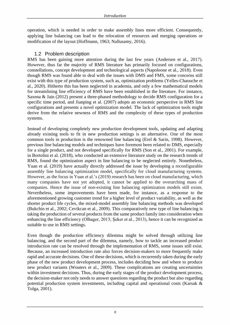
1.2 Problem description RMS has been gaining more attention during the last few years (Andersen et al., 2017).
However, thus far the majority of RMS literature has primarily focused on configurations,
constellations, concept development and technological aspects (Napoleone et al., 2018). Even
though RMS was found able to deal with the issues with DMS and FMS, some concerns still
exist with this type of production system, such as, optimization problems (Yelles-Chaouche et
al., 2020). Hitherto this has been neglected in academia, and only a few mathematical models
for streamlining line efficiency of RMS have been established in the literature. For instance,
Saxena & Jain (2012) present a three-phased methodology to decide RMS configuration for a
specific time period, and Jianping et al. (2007) adopts an economic perspective in RMS line
configurations and presents a novel optimization model. The lack of optimization tools might
derive from the relative newness of RMS and the complexity of these types of production
systems.
Instead of developing completely new production development tools, updating and adapting
already existing tools to fit in new production settings is an alternative. One of the most
common tools in production is the renowned line balancing (Erel & Sarin, 1998). However,
previous line balancing models and techniques have foremost been related to DMS, especially
for a single product, and not developed specifically for RMS (Son et al., 2001). For example,
in Bortolini et al. (2018), who conducted an extensive literature study on the research trends of
RMS, found the optimization aspect in line balancing to be neglected entirely. Nonetheless,
Yuan et al. (2019) have actually directly addressed the issue by developing a reconfigurable
assembly line balancing optimization model, specifically for cloud manufacturing systems.
However, as the focus in Yuan et al.’s (2019) research has been on cloud manufacturing, which
many companies have not yet adopted, it cannot be applied to the overarching mass of
companies. Hence the issue of non-existing line balancing optimization models still exists.
Nevertheless, some improvements have been made, for instance, as a response to the
aforementioned growing customer trend for a higher level of product variability, as well as the
shorter product life cycles, the mixed-model assembly line balancing methods was developed
(Bukchin et al., 2002; Cevikcan et al., 2009). This comparatively new type of line balancing is
taking the production of several products from the same product family into consideration when
enhancing the line efficiency (Olhager, 2013; Şeker et al., 2013), hence it can be recognized as
suitable to use in RMS settings.
Even though the production efficiency dilemma might be solved through utilizing line
balancing, and the second part of the dilemma, namely, how to tackle an increased product
introduction rate can be resolved through the implementation of RMS, some issues still exist.
Because, an increased introduction rate also forces decision-makers to more frequently make
rapid and accurate decisions. One of these decisions, which is recurrently taken during the early
phase of the new product development process, includes deciding how and where to produce
new product variants (Wouters et al., 2009). These complications are creating uncertainties
within investment decisions. Thus, during the early stages of the product development process,
the decision-maker not only needs to answer questions regarding the product but also regarding
potential production system investments, including capital and operational costs (Karsak &
Tolga, 2001).
Introduction
3
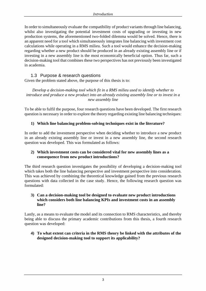
In order to simultaneously evaluate the compatibility of product variants through line balancing,
whilst also investigating the potential investment costs of upgrading or investing in new
production systems, the aforementioned two-folded dilemma would be solved. Hence, there is
an apparent need for a tool which simultaneously integrates line balancing with investment cost
calculations while operating in a RMS milieu. Such a tool would enhance the decision-making
regarding whether a new product should be produced in an already existing assembly line or if
investing in a new assembly line is the most economically beneficial option. Thus far, such a
decision-making tool that combines these two perspectives has not previously been investigated
in academia.
1.3 Purpose & research questions Given the problem stated above, the purpose of this thesis is to:
Develop a decision-making tool which fit in a RMS milieu used to identify whether to
introduce and produce a new product into an already existing assembly line or to invest in a
new assembly line
To be able to fulfil the purpose, four research questions have been developed. The first research
question is necessary in order to explore the theory regarding existing line balancing techniques:
1) Which line balancing problem-solving techniques exist in the literature?
In order to add the investment perspective when deciding whether to introduce a new product
in an already existing assembly line or invest in a new assembly line, the second research
question was developed. This was formulated as follows:
2) Which investment costs can be considered vital for new assembly lines as a
consequence from new product introductions?
The third research question investigates the possibility of developing a decision-making tool
which takes both the line balancing perspective and investment perspective into consideration.
This was achieved by combining the theoretical knowledge gained from the previous research
questions with data collected in the case study. Hence, the following research question was
formulated:
3) Can a decision-making tool be designed to evaluate new product introductions
which considers both line balancing KPIs and investment costs in an assembly
line?
Lastly, as a means to evaluate the model and its connection to RMS characteristics, and thereby
being able to discuss the primary academic contributions from this thesis, a fourth research
question was developed:
4) To what extent can criteria in the RMS theory be linked with the attributes of the
designed decision-making tool to support its applicability?
Introduction
4
1.4 Delimitations This thesis will solely focus on developing and analysing a decision-making tool from an RMS
perspective. Hence, other major production systems, i.e. DMS and FMS, will not be in focus.
Also, this thesis is only covers the development of a decision-making tool for straight line
layout assembly lines. Other types of assembly lines, such as U-lines are thereby excluded. This
delimitation was necessary since line balancing techniques and algorithms adapted for U-lines
are not identical to the ones for straight assembly lines. Furthermore, the validation and testing
of the decision-making tool (DMT) is based upon data provided from the case company. Thus,
the authors will not collect any time measurements by themselves and solely rely on the basis
that these are correct. Also, the decision-making tool will not be tested in a wider setting, with
input from other companies. Further delimitations regard that the report only covers KPIs
connected to line balancing and investment costs on an overarching level. This delimitation
exists since the decision-making tool is intended as being modular, whereas users have the
possibility to insert the most relevant KPIs and investment costs in their situation.
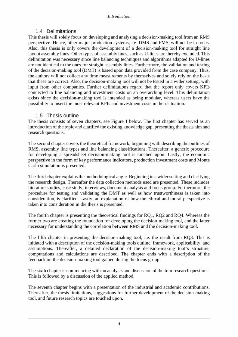
1.5 Thesis outline The thesis consists of seven chapters, see Figure 1 below. The first chapter has served as an
introduction of the topic and clarified the existing knowledge gap, presenting the thesis aim and
research questions.
The second chapter covers the theoretical framework, beginning with describing the outlines of
RMS, assembly line types and line balancing classifications. Thereafter, a generic procedure
for developing a spreadsheet decision-making tool is touched upon. Lastly, the economic
perspective in the form of key performance indicators, production investment costs and Monte
Carlo simulation is presented.
The third chapter explains the methodological angle. Beginning in a wider setting and clarifying
the research design. Thereafter the data collection methods used are presented. These includes
literature studies, case study, interviews, document analysis and focus group. Furthermore, the
procedure for testing and validating the DMT as well as how trustworthiness is taken into
consideration, is clarified. Lastly, an explanation of how the ethical and moral perspective is
taken into consideration in the thesis is presented.
The fourth chapter is presenting the theoretical findings for RQ1, RQ2 and RQ4. Whereas the
former two are creating the foundation for developing the decision-making tool, and the latter
necessary for understanding the correlation between RMS and the decision-making tool.
The fifth chapter in presenting the decision-making tool, i.e. the result from RQ3. This is
initiated with a description of the decision-making tools outline, framework, applicability, and
assumptions. Thereafter, a detailed declaration of the decision-making tool’s structure,
computations and calculations are described. The chapter ends with a description of the
feedback on the decision-making tool gained during the focus group.
The sixth chapter is commencing with an analysis and discussion of the four research questions.
This is followed by a discussion of the applied method.
The seventh chapter begins with a presentation of the industrial and academic contributions.
Thereafter, the thesis limitations, suggestions for further development of the decision-making
tool, and future research topics are touched upon.
Introduction
5
Figure 1 - Thesis structure and outline

Theoretical Framework
6
2 Theoretical framework
The second chapter covers the thesis theoretical framework, beginning with describing RMS
and associated classifications and characteristics. Thereafter, the line balancing and
investment costs theory is presented.
2.1 Reconfigurable manufacturing systems The complexity of modern industrial processes motivates the need to adapt a holistic
perspective when designing or operating production systems. The main concern is that many
researchers have underlined the interrelated relationship between the components and levels of
the system (Bellgran & Säfsten, 2009). For instance, Groover (2016) highlighted that the
production system consists of two core levels. One of these regard facilities, which include
factories, machinery, material handling tools and so on. The other level regards the
manufacturing support system, focusing on the soft part of the system. This includes standards,
procedures, product design, and working schedules, etc. Manufacturing systems can further be
categorized based on the systems’ flexibility to handle changes in demand. According to Koren
et al. (1999), manufacturing systems can be divided into three categories; DMS, FMS and RMS.
DMS are prepared with a set of machining and other material handling equipment which
facilitates delivery of a product with specific features. Such a system targets to produce in mass
capacity with very low variation in products or manufacturing process. The simplicity of the
system requires workers with a minimum degree of skill. As a result of this, dedicated
manufacturing systems are typically cost-effective when high demand with low product variety
is expected (Bellgran & Säfsten, 2009). On the other hand, FMS are equipped with machinery
which are able to handle products with a wide difference in features. This ability facilitates the
possibility to produce complex products, which is not easily accomplished in DMS. The FMS
usually contains CNC machines and a high level of automation. However, several drawbacks
related to FMS have appeared. These drawbacks primarily regard long setup time to change
between products and an extensive time-consuming maintenance (Koren et al., 2018).
Nevertheless, improvements have been introduced to both DMS and FMS in order to avoid the
lack of flexibility of the DMS and to increase the production capacity of FMS. These
improvements created a space of solutions that are defined as RMS, as illustrated in Figure 2
(Koren, 2006; Wiendahl et al., 2007).
Figure 2 - DMS, FMS and RMS, adapted from Koren (2006).

Theoretical Framework
7
RMS has further been presented as the hybrid system between DMS and FMS. This since RMS
brings together the benefits of having cost-effectiveness as a result of mass production and
responsiveness to change in features of the products within a product family (Koren &
Shpitalni, 2010).
2.1.1 RMS classification The competitiveness among industrial companies puts pressure on manufacturers to stay viable
and respond to customer demands. This in turn creates the necessity to frequently introduce
new products in existing production systems (Bellgran & Säfsten, 2009). Many researchers
have associated the development or change of the production system to match product
introductions, particularly RMS. For instance, Säfsten & Aresu (2000) conducted a survey on
15 companies. In the research, Säfsten & Aresu (2000) linked introducing new products to the
changes in assembly lines that give the companies the advantage of launching new products
before their competitors. Also, Surbier (2014) emphasized on the relation between production
ramp-up for new products and disturbances in product quality and assembly line performance.
Both studies can connect to the works of ElMaraghy (2006) and Koren & Shpitalni (2010) on
reconfigurability enablers. ElMaraghy (2006) identified two types of flexibility: physical and
logical. The physical aspect includes production layout, machines, and material handling
equipment, while the logical aspect includes for instance, production planning, human
resources, and rerouting (Figure 3).
Figure 3 - RMS soft and hard classification, based on ElMaraghy (2006).
Considering the abovementioned classifications, RMS can be supported through both physical
and logical aspects. For example, scaling up the production capacity can be achieved by adding
more machines to an existing production system. However, changing production planning or
product mix can lead to an increase in the volume without changing the physical structure of
the production system (ElMaraghy, 2006; Lohse et al., 2006; Mehrabi et al., 2000).
Furthermore, Wiendahl et al. (2007) argue that soft reconfigurability can be valuable to increase
cost efficiency and respond to the demand without investing in the new line features.
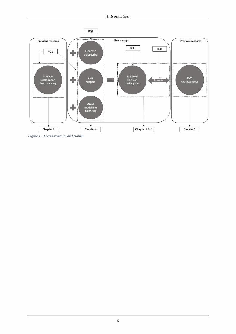
2.1.2 RMS characteristics Researchers have identified seven characteristics that enable the manufacturing system to
achieve reconfigurability, these are presented in Table 1 below based on (Koren et al., 1999;
Koren & Shpitalni, 2010; Maler-Speredelozzi et al., 2003; Naor et al., 2010; Rösiö et al., 2019;
Wiendahl et al., 2007; Youssef & Elmaraghy, 2006). However, it is important to note that
Theoretical Framework
8
researchers have identified RMS characteristics using different terms. For example, Wiendahl
et al. (2007) found mobility to be one of RMS characteristics , while Napoleone et al. (2018)
and Rösiö et al. (2019) did not acknowledge the term mobility but instead covered mobility
within other characteristics, namely as modularity and integrability.
Table 1 - RMS characteristics
Characteristic Definition Scalability Scalability of the system's production rate is required to respond to changes in demand in
a timely manner. Scalability encompasses both system scalability and capacity scalability.
The former, i.e., system scalability, refers to meeting market demand with the least
amount of system capacity growth. Capability flexibility, on the other hand, has two
components. One of these components is the physical flexibility of attaching and
disconnecting machines and material handling equipment to the production system. The
other component is logical flexibility and refers to the ability to extend production time
and increasing working shifts or manpower.
Customization The ability of a production system to respond to differences within the same product
family is referred to as customization. It is possible to use the same software to create
different features within the same product family using a customized configuration. To
allow system customization, there is also a need for software to track running mixed
products within the same line.
Convertibility Convertibility refers to a manufacturing system's ability to convert between various
configurations in order to meet fluctuating demand. When switching between product
variants and future models, a convertible development system requires the least amount
of setup time.
Modularity Production system modularity refers to the standardization of system components and
functions. Modularity allows for the replacement, removal, and addition of modules
without disrupting other components of the system. Modularity enables the
construction of complex systems that can react to changes in product features or
fluctuating demand.
Integrability Production system integrability, also known as compatibility, refers to the compatibility
of various applications, materials, and interfaces within the various components of a
production system. Integrability is critical for ensuring coordination between all
production system components at various stages of production. When a new component
is added to an existing system, it is critical to connect it logically and physically to the
current control system and production infrastructures. On a physical basis, integrability
enables newly connected components to send and receive goods and materials with ease.
Physical integrability involves exchanging data and control signals with other elements
of the production system, while logical integrability entails exchanging data and control
signals with other parts of the production process.
Diagnosability Diagnosability enables the manufacturing system to diagnose performance disturbances
rapidly and accurately within the production system. The system must quickly diagnose
equipment and material handling errors and assess their effect on the rest of the system.
Furthermore, diagnosability in manufacturing systems entails tracing product quality
issues and investigating root causes.
Mobility The freedom to transfer production system elements is referred to as mobility in the RMS.
This covers machines, facilities, and infrastructure. Mobility contributes to the system's
flexibility; unrestricted equipment can be quickly transported within the factory to expand
production capacity wherever there is a lack of production resources.
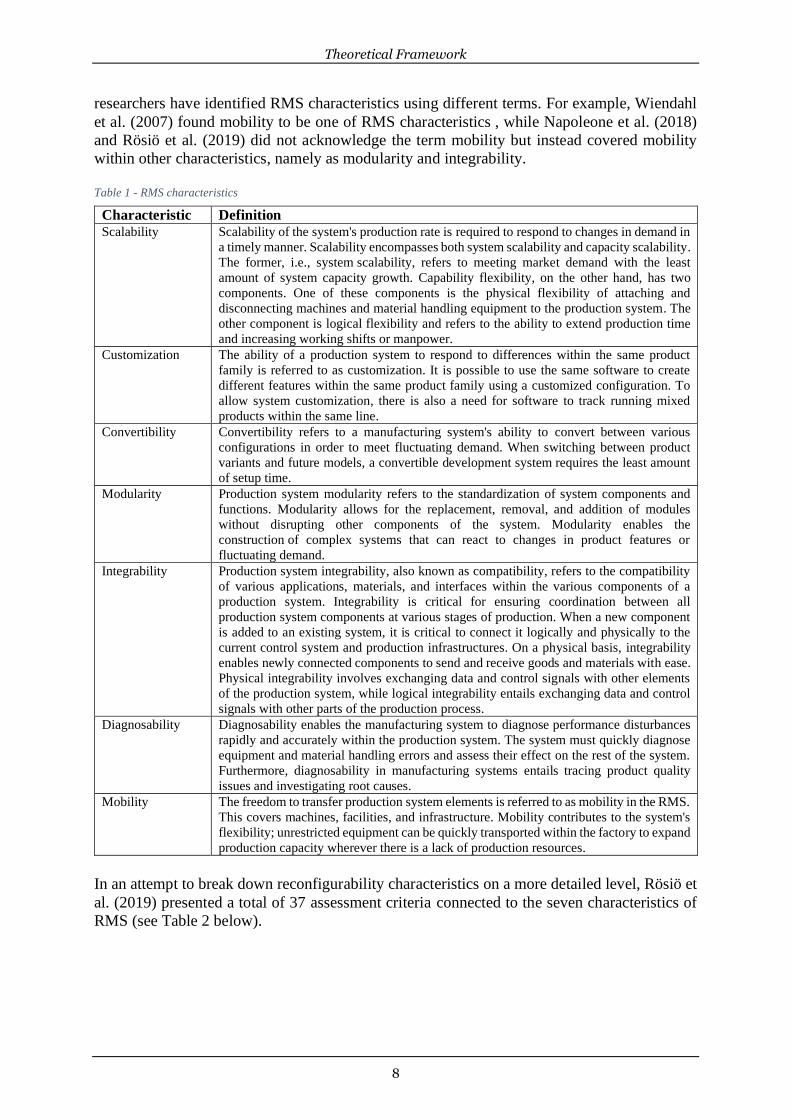
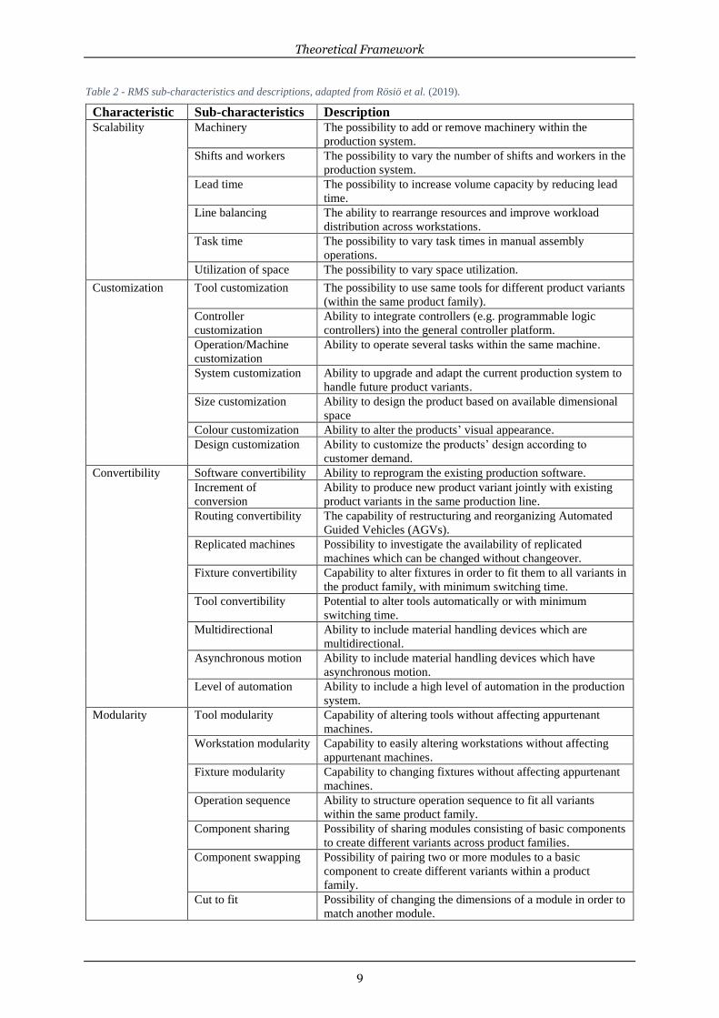
In an attempt to break down reconfigurability characteristics on a more detailed level, Rösiö et
al. (2019) presented a total of 37 assessment criteria connected to the seven characteristics of
RMS (see Table 2 below).
Theoretical Framework
9
Table 2 - RMS sub-characteristics and descriptions, adapted from Rösiö et al. (2019).
Characteristic Sub-characteristics Description Scalability Machinery The possibility to add or remove machinery within the
production system.
Shifts and workers The possibility to vary the number of shifts and workers in the
production system.
Lead time The possibility to increase volume capacity by reducing lead
time.
Line balancing The ability to rearrange resources and improve workload
distribution across workstations.
Task time The possibility to vary task times in manual assembly
operations.
Utilization of space The possibility to vary space utilization.
Customization Tool customization The possibility to use same tools for different product variants
(within the same product family).
Controller
customization
Ability to integrate controllers (e.g. programmable logic
controllers) into the general controller platform.
Operation/Machine
customization
Ability to operate several tasks within the same machine.
System customization Ability to upgrade and adapt the current production system to
handle future product variants.
Size customization Ability to design the product based on available dimensional
space
Colour customization Ability to alter the products’ visual appearance.
Design customization Ability to customize the products’ design according to
customer demand.
Convertibility Software convertibility Ability to reprogram the existing production software.
Increment of
conversion
Ability to produce new product variant jointly with existing
product variants in the same production line.
Routing convertibility The capability of restructuring and reorganizing Automated
Guided Vehicles (AGVs).
Replicated machines Possibility to investigate the availability of replicated
machines which can be changed without changeover.
Fixture convertibility Capability to alter fixtures in order to fit them to all variants in
the product family, with minimum switching time.
Tool convertibility Potential to alter tools automatically or with minimum
switching time.
Multidirectional Ability to include material handling devices which are
multidirectional.
Asynchronous motion Ability to include material handling devices which have
asynchronous motion.
Level of automation Ability to include a high level of automation in the production
system.
Modularity Tool modularity Capability of altering tools without affecting appurtenant
machines.
Workstation modularity Capability to easily altering workstations without affecting
appurtenant machines.
Fixture modularity Capability to changing fixtures without affecting appurtenant
machines.
Operation sequence Ability to structure operation sequence to fit all variants
within the same product family.
Component sharing Possibility of sharing modules consisting of basic components
to create different variants across product families.
Component swapping Possibility of pairing two or more modules to a basic
component to create different variants within a product
family.
Cut to fit Possibility of changing the dimensions of a module in order to
match another module.
Theoretical Framework
10
Bus modularity Possibility to match disparate modules to a basic component.
Integrability Tool integrability Capability to integrate new tools in existing machines in the
production system.
Control software Capability to integrate already existing control software into
new tools and machines.
Information handling
integrability
Capability to integrate information with new work tasks in the
production system.
Diagnosability Poka yoke The capability to detect the usage of correct tool and
components for the product family variants.
Information board The ability to display the upcoming operation on the focal
machine or assembly line.
Traceability The ability to trace the product’s current production
stage/operation.
Quality assurance The ability to immediately detect unsatisfactory product
quality through visual technology (e.g. cameras and sensors).
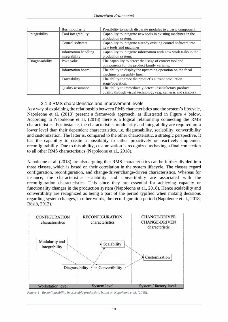
2.1.3 RMS characteristics and improvement levels As a way of explaining the relationship between RMS characteristics and the system’s lifecycle,
Napoleone et al. (2018) present a framework approach, as illustrated in Figure 4 below.
According to Napoleone et al. (2018) there is a logical relationship connecting the RMS
characteristics. For instance, the characteristics modularity and integrability are required on a
lower level than their dependent characteristics, i.e. diagnosability, scalability, convertibility
and customization. The latter is, compared to the other characteristic, a strategic perspective. It
has the capability to create a possibility to either proactively or reactively implement
reconfigurability. Due to this ability, customization is recognized as having a final connection
to all other RMS characteristics (Napoleone et al., 2018).
Napoleone et al. (2018) are also arguing that RMS characteristics can be further divided into
three classes, which is based on their correlation in the system lifecycle. The classes regard
configuration, reconfiguration, and change-driver/change-driven characteristics. Whereas for
instance, the characteristics scalability and convertibility are associated with the
reconfiguration characteristics. This since they are essential for achieving capacity or
functionality changes in the production system (Napoleone et al., 2018). Hence scalability and
convertibility are recognized as being a part of the period typified when making decisions
regarding system changes, in other words, the reconfiguration period (Napoleone et al., 2018;
Rösiö, 2012).
Figure 4 - Reconfigurability in assembly production, based on Napoleone et al. (2018).

Theoretical Framework
11
Napoleone et al. (2018) also describe that the lowest level to find the RMS characteristics
modularity, integrability and diagnosability is on an assembly station level. Due to the position
of these characteristics being at a workstation level (e.g. assembly station), i.e. the most
concrete level, the characteristics convertibility and scalability are at the possible to achieve on
a system level (e.g. cells, production lines or assembly systems). This enables a possibility to
achieve customization on both system and factory levels (Napoleone et al., 2018).
2.2 Single-, mixed- & multi-model assembly lines Assembly lines were famously introduced by Henry Ford in the beginning of the twentieth
century. Assembly lines are setups for manufacturing processes where value is added to
products, for instance in terms of operations performed or subparts added. Traditionally,
workstations where these operations occur are logically placed in a predetermined sequence
and placed in proximity to each other. However, conveyor belts or similar transportation
systems are also solutions frequently used when necessary. At the workstations, humans or
machines are to perform a predetermined set of operations which they complete before the
product is transported to the subsequent workstation (Fortuny-Santos et al., 2020). Since
assembly lines can be comprised of machines, tools and human labour, while being quite
extensive, they are associated with a high level of investment costs (Alghazi & Kurz, 2018;
Fortuny-Santos et al., 2020). This puts an emphasis for companies on establishing a proper
configuration of assembly lines (Alghazi & Kurz, 2018).
Originally, assembly lines were implemented as a means for companies to accomplish mass
production of identic products while staying cost-efficient (Alghazi & Kurz, 2018; Fortuny-
Santos et al., 2020). However, in line with organisational and technological development,
assembly lines have developed and nowadays several products can be assembled in the same
assembly line (Fortuny-Santos et al., 2020). The configurations of product and assembly lines
can be divided into three main categories; single-model assembly lines, mixed-model assembly
lines and single-model assembly lines (see Figure 5 below) (Güden & Meral, 2016; Olhager,
2013; Şeker et al., 2013).
Single-model assembly lines are the least complex assembly line. These are commonly
implemented in mass production facilities. Primarily since they traditionally enable the
possibility of having operators with little training to manually assemble complex and detailed
products (Cevikcan et al., 2009).
Figure 5 - Different assembly lines types, adapted from Olhager (2013).
Mixed-model assembly lines (MMALs), on the other hand, are used to manufacture several
products within the same product family (Akpinar et al., 2017; Olhager, 2013). These are
simultaneously assembled on the same line (Mirzapour Al-E-Hashem et al., 2009). In MMALs,
each specific product variant has its own task precedence rules, which are combined into a
Theoretical Framework
12
precedence diagram of the entire product family (Akpinar et al., 2017). MMALs are frequently
used in car-manufacturing facilities as these tend only to produce a limited fixed set of product
families. Normally, these do not require any machine- or tool setup between different product
variants. However, there is a higher level of complexity in material- and component handling
in MMALs as they need to serve the needs of several models simultaneously (Olhager, 2013).
The third category of assembly lines is multi-model assembly lines. If the products assembled
in the production line are of comprehensive difference, setup time might be required between
producing the products in sequence. Thus, the key question when producing in multi-model
assembly lines regards whether the products have a sufficient similarity level in terms of
components and production resources in order to be economically beneficial (Olhager, 2013).
2.3 Line balancing problems Assembly lines were initially intended to produce a limited variety of products in large
quantities. A setup like this allows low production costs, short cycle times, and high quality.
However, due to the high capital cost needed to build and operate an assembly line,
manufacturers produce one product with various features or several products within the same
product family on a single assembly line simultaneously (Bellgran & Säfsten, 2009). Producing
or assembling of a product often requires several operations. Seldom are these operations
unidentical and require various time for completion, a workload varies among employees and
stations due to the different operating times. As a result, the aim is to delegate the same
workload to all employees or computers. To provide a smooth work distribution within
assembly lines, two aspects need to be considered: 1) The total number of workstations must
be kept to the minimum, 2) The logical precedence constraints that must be followed. The latter
aspect is required since some of the processes cannot be performed before their predecessors
(Groover, 2016; Watanabe et al., 1995). Furthermore, there is a set of assumptions that need to
be considered in solving assembly line balancing problems (ALBP), the assumptions decide
the input data, techniques, and the final solutions for the problem. Although the final goal for
all ALBP is to reach a feasible work distribution, the method is different based on the line
characteristics, such as the number of products per line, the pre-determined number of
workstations, or task time (Battaïa & Dolgui, 2013).
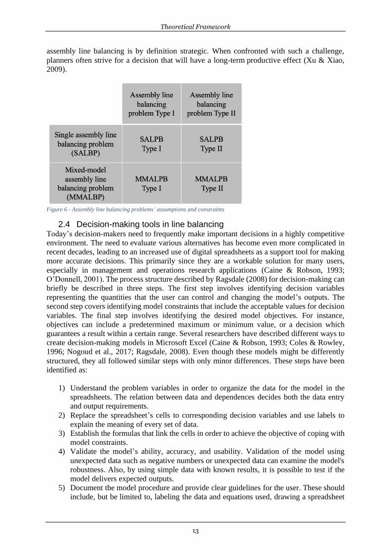
When deciding which strategy to use to solve ALBP, some assumptions about the assembly
line must be considered. As an example, assumptions on the number of models to be
manufactured are referred to as single assembly line balancing problems (SALBP) in the case
of a single model product, while mixed-model assembly line balancing problems (MMALBP)
are problems with two or more products produced on the same line (Mirzapour Al-E-Hashem
et al., 2009).
Another assumption to note is the objective of the balancing, whether it is to minimize the
number of stations or to increase throughput by reducing the cycle times of the assembly
activities. Thus, ALBP type I aims to reduce the number of stations or staff needed to meet the
output demand where the process time is set. ALBP Type II, on the other hand, aims for the
maximum output rate and the shortest cycle time while maintaining a constant number of
workstations. Regardless of the distinction between the two, both assume that the operating
time allotted to stations does not exceed the cycle time of the assembly line (Becker & Scholl,
2006; Rabbani et al., 2016).
However, these assumptions are not separated, see Figure 6, and it is critical to consider all of
the assembly line constraints and objectives when agreeing on the best strategy. This since
Theoretical Framework
13
assembly line balancing is by definition strategic. When confronted with such a challenge,
planners often strive for a decision that will have a long-term productive effect (Xu & Xiao,
2009).
Figure 6 - Assembly line balancing problems’ assumptions and constraints
2.4 Decision-making tools in line balancing Today’s decision-makers need to frequently make important decisions in a highly competitive
environment. The need to evaluate various alternatives has become even more complicated in
recent decades, leading to an increased use of digital spreadsheets as a support tool for making
more accurate decisions. This primarily since they are a workable solution for many users,
especially in management and operations research applications (Caine & Robson, 1993;
O’Donnell, 2001). The process structure described by Ragsdale (2008) for decision-making can
briefly be described in three steps. The first step involves identifying decision variables
representing the quantities that the user can control and changing the model’s outputs. The
second step covers identifying model constraints that include the acceptable values for decision
variables. The final step involves identifying the desired model objectives. For instance,
objectives can include a predetermined maximum or minimum value, or a decision which
guarantees a result within a certain range. Several researchers have described different ways to
create decision-making models in Microsoft Excel (Caine & Robson, 1993; Coles & Rowley,
1996; Nogoud et al., 2017; Ragsdale, 2008). Even though these models might be differently
structured, they all followed similar steps with only minor differences. These steps have been
identified as:
1) Understand the problem variables in order to organize the data for the model in the
spreadsheets. The relation between data and dependences decides both the data entry
and output requirements.
2) Replace the spreadsheet’s cells to corresponding decision variables and use labels to
explain the meaning of every set of data.
3) Establish the formulas that link the cells in order to achieve the objective of coping with
model constraints.
4) Validate the model’s ability, accuracy, and usability. Validation of the model using
unexpected data such as negative numbers or unexpected data can examine the model's
robustness. Also, by using simple data with known results, it is possible to test if the
model delivers expected outputs.
5) Document the model procedure and provide clear guidelines for the user. These should
include, but be limited to, labeling the data and equations used, drawing a spreadsheet
Theoretical Framework
14
map, and clarifying the formulas.
6) Implement the model and receive early feedback from the users to optimize the model
in order to reach the desirable results.
2.5 Line balancing models and computation Microsoft Excel spreadsheets have been the most widely used tools in recent decades when it
comes to operation analysis and solving project management network problems (Caine &
Robson, 1993). Ragsdale and Brown (2004) created one of the first models which use Microsoft
Excel spreadsheets to explain and solve predecessor relations between tasks. About a decade
later, both Weiss (2013) and Wellington & Lewis (2018) extended the previous work in a new
area of application through the use of a heuristic approach to solve line balancing problems for
a single model product. Their work shares the same basic structure, which can be divided into
two major steps. The first step regards identifying the assembly line parameters in the form of
a table. This table includes inserting the values of task names, task times (operations time),
required cycle time (operations time) and immediate predecessors between tasks (Weiss, 2013;
Wellington & Lewis, 2018).
The second step is to identify the workstations’ feasibility based on two requirements. Firstly,
all previous operations have been assigned to the available stations. Secondly, the sum of task
times is less than or equal to the theoretical maximum time required to produce one product
through the assembly line. Following that, the task is allocated in accordance with the existing
priority rule. For every iteration, a single task is considered at a time. The computation of the
process is achieved through combinations of built-in functions in Microsoft Excel. The coding
system is structured in such a way that it automatically allocates tasks to stations by assigning
0 for tasks which have not been assigned yet, and -1 to tasks which have been assigned to
previous stations. This allows the spreadsheet to identify the first task to start with it and to stop
the computation when no more task is available. The spreadsheet checks if the activity code is
0 and then checks if the available time in the station is less than the operating time using the
built-in Microsoft Excel IF functions. In the case when all conditions are met, the sheet subtracts
the task (operation) time from the station time and keeps the remaining time to be set as the
current overall available time. Thereafter the sheet changes the code of the task to be -1 or less.
Once this has been accomplished, a new iteration starts by checking if the next task code is
equal to 0. (Weiss, 2013; Wellington & Lewis, 2018). Some common Microsoft Excel formulas
frequently used by Caine & Robson (1993), Ragsdale & Brown (2004) and Wellington & Lewis
(2018) are:
- IF: check the logical conditions for a priority rule and station availability through the
mathematical denotations “<” “>” “=”.
- SUM: at each iteration, the SUM-function is used to count the number of tasks that fulfil
the requirement and thereafter returns the task code for the new iteration.
- SEARCH: maintain the task code with a combination of IF conditional functions.
- VLOOKUP: searches for a certain task name and time with the task code in the inputs.
- OFFSET: used for dynamic functions where there is a need to return a value based on a
reference cell. The OFFSET-function is used in order for tasks to be assigned based on
the line balancing priority rules.

Theoretical Framework
15
2.6 Key performance indicators in line balancing A key performance indicator (KPI) is defined as a comparable value or number which is used
to gain insight into a certain performance. The KPI can be compared to either a selected internal
target or an external target. The number or value in the KPI consists of either collected or
calculated data (Ahmad & Dhafr, 2002). In regard to assembly lines, there are two main types
of KPIs. These differ based upon time perspective. The KPIs which are reporting an assembly
line’s current status and performance is referred to as online KPIs. Operators and managers
frequently use these to ease decision-making regarding assembly line improvements or
problems in need of instantaneous alteration. On the other side of the time perspective, offline
KPIs are indicators of an assembly line’s performance calculated or collected based on
historical data. Hence offline KPIs are more frequently used by managers when the aim is to
proactively identify problems in the assembly lines and thereby enable the possibility of
constructing action plans to avoid the identified problems in the future (Mohammed & Bilal,
2019).
Hitherto, many authors have tried to solve the issues in line balancing. Both regarding the
simple assembly line balancing problems or more complicated assembly line which produces
multiple products within the same line, for instance McMullen & Tarasewich (2003), Su et al.
(2014) and Samouei (2019). With this, new algorithms and techniques have been developed.
Consequently, the usage of KPIs has also been developed. When Salveson (1955) first
introduced line balancing, the KPIs used were cycle time, throughput time, idle time, machine
utilization and balancing loss. Nowadays the KPIs tend to be more advanced, for instance taking
shape in the form of flexibility of staff, process planning, market requirements (März, 2012)
and planned order execution time (Ferrer et al., 2018).
2.7 Assembly line investment costs Investments, for instance regarding production and assembly line, is a critical factor of a
company's long-term economic performance. Once a decision has been made, it is seldom
possible to reverse the actions taken (Nickell, 1978). However, many organisations, both within
the public and private sectors, still base their investment on the initial purchase costs, without
any consideration of the assets’ life span and discount rate. In order to cope with these factors,
and thus facilitate a more realistic financial outcome, investment calculation methods such as
Life Cycle Cost (LCC) techniques and calculations have been developed (Woodward, 1997).
LCC techniques are particularly widespread as they optimize the total cost of ownership by
taking a wide range of technical data into consideration (Tosatti, 2006; Woodward, 1997)
Similar to the principle of LCC calculations, the Net Present Value (NPV) method is also taking
the discounting cash flows over a certain time-line into consideration in the investment
decision. Although, in contrast, NPV is typically used in business planning and for making
strategic decisions. In contrast, LCC techniques on the other hand are intended for enabling a
comparison of the anticipated economic lifecycle performance of investment alternatives, for
instance regarding production systems (Tosatti, 2006; Woodward, 1997).
2.8 Monte Carlo simulations The Monte Carlo simulation method’s origin dates back to the 1940s (Platon & Constantinescu,
2014). However, it was not until 40 years later when Monte Carlo simulations started receiving
concentrated attention from academia (Kelliher & Mahoney, 2000). Since then, they have been
used by professionals in a wide arrange of settings, for instance, in finance, project management
and production (Khalfi & Ourbih-Tari, 2020; Wang, 2012). The Monte Carlo method is a
computerized simulation technique which allows the user to analyze the entire range of possible

Theoretical Framework
16
outcomes and the impact of existing risks and uncertainties. Hence, the user is able to identify
key insights regarding the relationship between inputs and outcomes and thus enable better
decision making when uncertainty is present (Kelliher & Mahoney, 2000; Khalfi & Ourbih-
Tari, 2020; Saipe, 1977). Monte Carlo simulations are primarily useful since they are easy to
perform, but also due to their ability to provide the user with the possibility of running
thousands of iterations very quickly. (Kelliher & Mahoney, 2000; Platon & Constantinescu,
2014).
As aforementioned, Monte Carlo simulations are useful in many situations, none the least in
investment calculations. This since the key difference between Monte Carlo simulations and
other modeling techniques is their ability to not require certainty or normality in the inputs
(Kelliher & Mahoney, 2000), which is a frequent issue in investment decision making (Platon
& Constantinescu, 2014). In investments, Monte Carlo simulations can be used to calculate
possible outcomes when uncertainty in input values has a great impact on the final results
(Kelliher & Mahoney, 2000). According to Platon and Constantinescua (2014), one of the most
interesting research on Monte Carlo simulations was conducted by Dienemann in 1966 and
regarded cost estimating the uncertainty of investment projects. In more recent days, Monte
Carlo simulation to calculate investment decisions with an intrinsic uncertainty has been, for
instance, tested by Hacura et al. (2001). In their research, they used investment expenditures
connected to purchasing a new production facility, including building costs, technical
equipment, assembly work, and current assets (Hacura et al., 2001). Which showed how the
performance is influenced by the variation of certain cost and demand scenarios (Renna, 2017).
Furthermore, the number of iterations required to run Monte Carlo simulations is significant in
order to get viable results. Hauck & Anderson (1984) argued that the majority of studies on
Monte Carlo simulations have chosen to run between 500 and 1000 iterations. This
argumentation corresponds to, for instance, Caralis et al. (2014), who run several Monte Carlo
simulations in their research, whereas the most extensive consisted of 1000 iterations.

Methodology
17
3 Methodology The third chapter covers the methodology, beginning with explaining the research design.
Afterward follows a description regarding the usage of literature studies, case study,
interviews, document analysis and focus group in the thesis. Thereafter, the model validation
procedure is presented. Lastly, the trustworthiness, ethical- and moral perspective is declared
for.
3.1 Research design The thesis purpose was to “Develop a decision-making tool which fit in a RMS milieu used to
identify whether to introduce and produce a new product into an already existing assembly line
or to invest in a new assembly line”. Given the purpose, the nature of the thesis is equivalent to
exploring and explaining. These attributes correspond to a qualitative research approach (Leedy
et al., 2019). The qualitative approach is namely characterized as having flexible guidelines
which were necessary since the outcomes were not predetermined, but instead explorative.
Also, the data necessary to answer the research questions was collected in a small sample and
through, for instance, non-standardized interviews and document studies, which corresponds
well to the natural characteristics of a qualitative approach (Leedy et al., 2019).
In order to fulfil the purpose, four research questions was created. RQ1 and RQ2 were necessary
to answer in order to create the theoretical foundation for creating the decision-making tool.
Whilst in RQ3 the theoretical knowledge was combined with empirical data and thus enabled
the possibility to secure the applicability of the decision-making tool in an industry setting. In
order to validate the decision-making tool from an RMS perspective, and thereby illustrate how
the decision-making tool is supporting RMS, RQ4 was created. The connections between
research questions and methods used are depicted in Figure 7.
Figure 7 - Research design, adapted from Kovács & Spens (2005).

Methodology
18
3.2 Literature studies Since this thesis is covering a topic which thus far has been overlooked by academia, the need
to create a theoretical foundation for the DMT to stand upon is crucial. Therefore, several
extensive literature studies have been conducted. The literature studies have been structured to
focus on certain topics, these regarded RMS, line balancing, and assembly line investment
costs. By doing this, sufficient knowledge regarding the topics to create and evaluate the DMT
was gained. The literature studies took place in the shape of systematic reviews. This due to the
fact that a systematic review is appropriate to use when the goal is to draw a conclusion
regarding what is both known and unknown within a particular topic (Denyer & Tranfield,
2009; Saunders et al., 2016). This is corresponding well to the limited research previously
conducted on RMS and line balancing, as seen in Table 3 below. Besides, the systematic
literature review also has an increased internal validity due to its ability to minimize potential
biases such as selection bias and publication bias. The former regards researchers tend to choose
articles which correlate with his or her existing belief (Booth et al., 2016). The latter occurs
when, for instance, reviewers or editors act indifferently dependent on the direction or strength
of the focal article's findings (Booth et al., 2016; Gilbody & Song, 2000).
The literature studies were carried out through a five-step process, inspired by Booth et al.
(2016). The process is depicted in Figure 8 below. All searches were carried out in the abstract
and citation database Scopus. The initial searches were based on carefully selected
combinations of keywords. In order to exclude non-relevant papers, search filters were used.
The filters primarily involved limiting the searches to papers written in English and excluding
non-relevant fields such as environmental science, physics, and chemical engineering. The
filters also included limiting the searches to document types such as articles, books, and
conference papers. Once the filters were applied, the process was initiated with the first reading
round, where the abstract was read, and the papers reckoned relevant were selected. The second
reading round incorporated quickly reading the papers, and thereafter selecting the most
relevant papers to the third and final selection round. This round included reading the articles
once more in detail, while taking notes, excerpting quotes, and highlighting relevant findings.
Figure 8 - The applied process for the literature studies

Methodology
19
In total, three literature studies were conducted. One of the literature studies covered the
hitherto conducted research on RMS and line balancing. This literature study was performed
with the aim of gaining full insight into the current research on RMS and line balancing. In
particular how other researchers have adapted line balancing tools to fit RMS. However, as
seen in Table 3 below, the hits of searching for RMS and Line balancing were very few, proving
the limited research within the areas. This literature study also covered searching for typical
characteristics related to RMS, as a way of enabling the possibility to test the correlation
between RMS and the developed decision-making tool.
A literature study covering line balancing was also conducted. This was performed to create a
theoretical foundation for the thesis, as well as finding possible line balancing techniques and
algorithms necessary to create the decision-making tool. Even though there might be a clear
knowledge gap about the application of line balancing in RMS, as aforementioned, the need to
identify which line balancing techniques that can be used in RMS was necessary. A numerous
amount of algorithms and techniques were identified, however, the majority of these were either
too complicated to apply in a wider industry setting, or too mathematically complex to transfer
into a Microsoft Excel file.
Lastly, a literature study focusing on assembly line investment costs was conducted. By
identifying investment costs frequently used when estimating costs for new product
introductions, the authors were able to design the decision-making tool with the possibility of
including these in mind. As seen in Table 3, the initial search for assembly line investment costs
only resulted in a single hit, which forced broader searches within the field.
Table 3 - Applied keywords and search results in the literature studies
Theoretical topic Keywords Hits Incl.
filters
RMS "Reconfigurable manufacturing system*" AND ("Characteristic*"
OR "Criteria*" OR "Driver*" OR "Enabler*")
215 177
"Reconfigurable manufacturing system" OR "RMS" AND "Line
balancing"
10 9
"Reconfigurable manufacturing system*" OR "RMS" AND "Mixed-
model assembly line*"
4 4
Line balancing "Mixed model assembly line balancing" 140 118
"Mixed-model assembly lines" AND "Line balancing" 241 192
"Multi-model assembly line*" 32 29
"Line balancing" AND Algorithm* 1229 234
"Line balancing" AND Technique* 373 117
"Line balancing" AND "Decision making tool" 2 2
Assembly line
investment costs
"Assembly line*" AND Investment* AND ("New product
introduction*" OR NPI)
1 1
"Assembly line*" AND Investment* 214 156
Investment* AND Costs* AND Calculation* AND
(Production OR Manufacturing)
607 212
Methodology
20
3.3 Case study The aim of this research was to develop a decision-making tool which provides companies with
the possibility to scientifically calculate whether it is economically beneficial to produce the
new product in an already existing assembly line, or to invest in a completely new assembly
line. Hence, ensuring the industrial application of the tool is crucial for the research's relevance.
In order to achieve this, a single case study was conducted. The case study method was chosen
since it is an empirical method that is used when investigating an in-depth and realistic case
(Yin, 2018), thus making it a suitable choice for developing, testing and validating the DMT.
Also, by conducting the case study in parallel to designing the decision-making tool, the
possibility of continuously validating the DMT’s industrial application existed.
Nevertheless, there are a few downsides with using case studies. For instance, case studies
seldom have a distinct purpose. If studies have stated a clear purpose, then the problem instead
frequently relates to authors not being able to describe how the purpose is addressed in the study
(Corcoran et al., 2004). In order to deal with these issues, the purpose has been well-defined,
and research questions have been formulated carefully to support the purpose. Another
downside of case studies is that they require data from multiple sources. Therefore, the collected
data needs to be congregated through triangulation (Yin, 2018). This has been accomplished by
using three different data collecting methods in the case study: interviews, document analysis
and focus group. Below follows a detailed explanation of how these methods have been utilized.
3.3.1 Interviews In case studies, the interview method is one of the most significant information sources (Tellis,
1997; Williamson, 2002), hence it was used in this study. The interviews took place in the form
of bi-weekly meetings with a production engineer at the case company. Since the focus of the
interviews was to gain information about certain areas and topics, rather than about the
respondent, the interview was a viable method (Alvesson, 2011). According to Patel &
Davidson (2011), interviews can take place in different styles, primarily depending on their
structure and level of standardization. The interviews in this research were conducted as
discussions, whereas solely a few questions and the to be discussed topic was prepared
beforehand. These discussions, characterized by a low level of standardization and structure,
corresponds to unstructured interviews, as described by Patel & Davidson (2011). Performing
unstructured interviews was chosen as they are typically used when aiming to gain a deeper
understanding of a topic which a certain person possesses (Patel & Davidson, 2011). The
information retrieved from the interviews was in turn used to develop the decision-making tool.
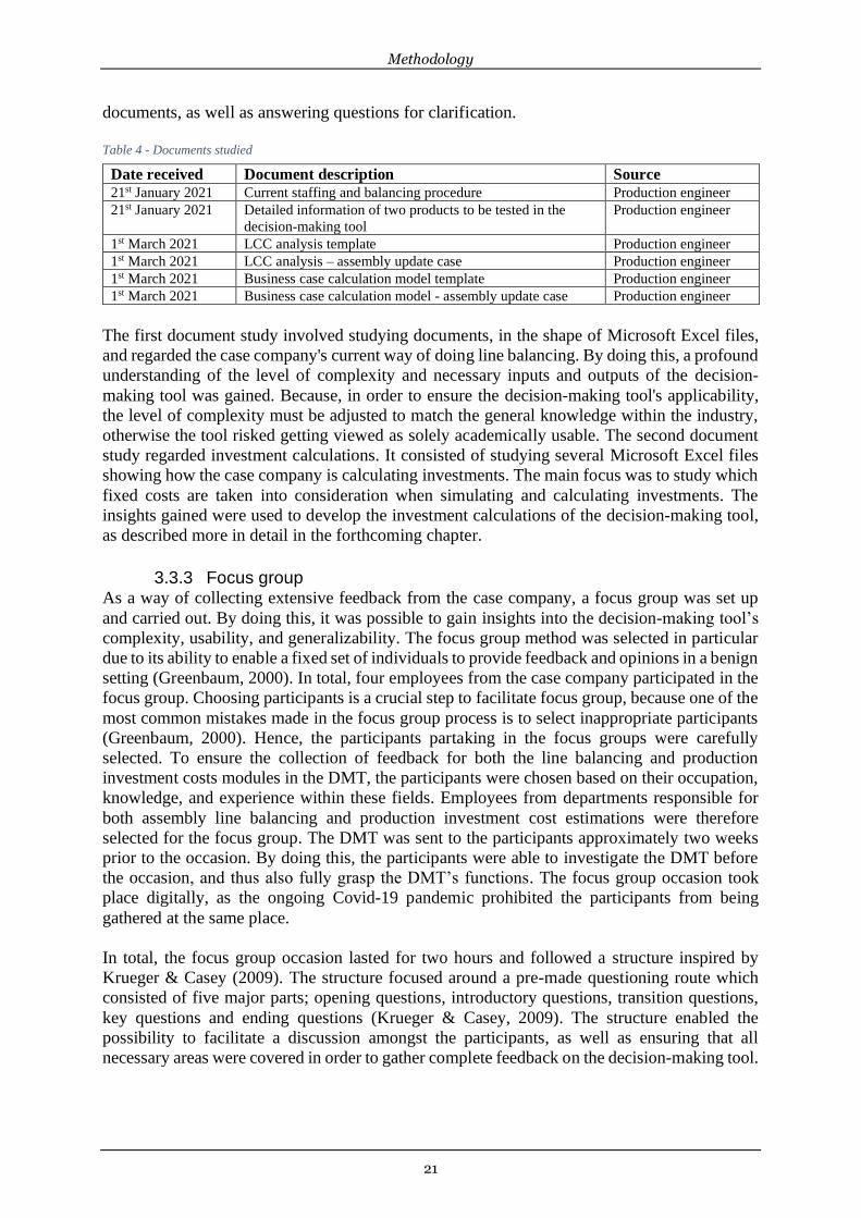
3.3.2 Document studies Document studies were carried out through the process of extracting data and information from
existing documents, and thus enabling the possibility to design, test and validate the decision-
making tool from an industry point of view. Document studies were chosen since they are an
adequate complement to other methods, for instance, literature studies and interviews (Skärvad
& Lindahl, 2016). In total, two document studies were performed, and a total of 6 documents
were reviewed. For both studies, the documents were sent via e-mail by a production engineer
at the case company (see Table 4). The authors were thus able to study the documents in their
own pace, potentially increasing the likelihood of properly understanding the data. This was
crucial since it is significant to interpret internal documents carefully in document studies. The
significance stems from the existing probability that the company has altered certain data, and
thus is not fully representative of the actual current state (Yin, 2018). Also, to further minimize
this risk of misreading data, interviews were carried out after performing the document studies.
These incorporated the company representative explaining the general content of the
Methodology
21
documents, as well as answering questions for clarification.
Table 4 - Documents studied
Date received Document description Source 21st January 2021 Current staffing and balancing procedure Production engineer
21st January 2021 Detailed information of two products to be tested in the
decision-making tool
Production engineer
1st March 2021 LCC analysis template Production engineer
1st March 2021 LCC analysis – assembly update case Production engineer
1st March 2021 Business case calculation model template Production engineer
1st March 2021 Business case calculation model - assembly update case Production engineer
The first document study involved studying documents, in the shape of Microsoft Excel files,
and regarded the case company's current way of doing line balancing. By doing this, a profound
understanding of the level of complexity and necessary inputs and outputs of the decision-
making tool was gained. Because, in order to ensure the decision-making tool's applicability,
the level of complexity must be adjusted to match the general knowledge within the industry,
otherwise the tool risked getting viewed as solely academically usable. The second document
study regarded investment calculations. It consisted of studying several Microsoft Excel files
showing how the case company is calculating investments. The main focus was to study which
fixed costs are taken into consideration when simulating and calculating investments. The
insights gained were used to develop the investment calculations of the decision-making tool,
as described more in detail in the forthcoming chapter.
3.3.3 Focus group As a way of collecting extensive feedback from the case company, a focus group was set up
and carried out. By doing this, it was possible to gain insights into the decision-making tool’s
complexity, usability, and generalizability. The focus group method was selected in particular
due to its ability to enable a fixed set of individuals to provide feedback and opinions in a benign
setting (Greenbaum, 2000). In total, four employees from the case company participated in the
focus group. Choosing participants is a crucial step to facilitate focus group, because one of the
most common mistakes made in the focus group process is to select inappropriate participants
(Greenbaum, 2000). Hence, the participants partaking in the focus groups were carefully
selected. To ensure the collection of feedback for both the line balancing and production
investment costs modules in the DMT, the participants were chosen based on their occupation,
knowledge, and experience within these fields. Employees from departments responsible for
both assembly line balancing and production investment cost estimations were therefore
selected for the focus group. The DMT was sent to the participants approximately two weeks
prior to the occasion. By doing this, the participants were able to investigate the DMT before
the occasion, and thus also fully grasp the DMT’s functions. The focus group occasion took
place digitally, as the ongoing Covid-19 pandemic prohibited the participants from being
gathered at the same place.
In total, the focus group occasion lasted for two hours and followed a structure inspired by
Krueger & Casey (2009). The structure focused around a pre-made questioning route which
consisted of five major parts; opening questions, introductory questions, transition questions,
key questions and ending questions (Krueger & Casey, 2009). The structure enabled the
possibility to facilitate a discussion amongst the participants, as well as ensuring that all
necessary areas were covered in order to gather complete feedback on the decision-making tool.
Methodology
22
3.4 Case company context The case company’s current product industrialization process starts with a product design, after
which the product features and requirements are developed and submitted to production
planning personnel. During this stage, the data available from the data management system is
used as an input for AVIX software to conduct time studies and calculate the process time
required to perform all assembly activities. During the assembly planning, current assembly
lines are used as guides to measure the movement times required to complete the assembly task,
as well as the setup time needed to change the line setup to receive the new product variant’s
task times. Based on previous experience and estimations from assembly planning employees,
this data is used to create line balancing using one of the line balancing techniques. However,
these estimates are not precise since they are dependent on several uncertainties and cover only
one balancing technique. The next step in the procedure is to identify the new line’s
requirements based on preliminary investment cost estimates. Nevertheless, product features
may be modified to match current assembly lines, otherwise, data may be submitted to suppliers
to provide appropriate solutions. Consequently, there is a high degree of uncertainty in the
current product industrialization process, especially as new product variants are to be produced
alongside other product variant in the same assembly lines.
3.5 Model validation and testing The validation and testing of the DMT were based on Caine & Robson’s (1993) three step
validation process. This process was selected because it was explicitly developed for
spreadsheet models, which is the base of the developed DMT. In the process, the first step
involves inserting incorrect data into the model in order to test its robustness. This is particularly
important if the model is intended for third-party usage (Caine & Robson, 1993). For this thesis,
this was accomplished by inserting already known incorrect data. The impacts were then
studied, and appropriate changes and features were added to the decision-making tool. For
instance, one of the changes related to this step regards the implementation of an IFerror
function in order to avoid incorrect data entry. If the result of the task is an error value at any
stage during the iterations, the IFerror-function returns the value zero or a blank cell, instead of
ending the calculations. Also, the implementation of instructions provides vital information to
the user for how to reduce wrong data entry. Furthermore, with the aim of minimizing wrong
data entry, colour coding highlighting in which cells the user are supposed to enter values was
used.
The second step involves verifying the model, which implies checking the logical relations
between the different spreadsheets and ensuring the accuracy of the intermediate and final
results (Caine & Robson, 1993). To verify the decision-making tool’s accuracy, an already
conducted mixed-model assembly line balancing process presented by Groover (2016) was
decomposed into comparable steps. The input data from Groover‘s (2016) calculation was then
used in the decision-making tool. Both the intermediate outputs and final outputs of the
decision-making tool were then traced through the spreadsheets and compared with the
expected results in Groover’s (2016) calculations. By following this procedure, with already
known correct outcomes, it was possible to easily identify any unexpected and undesired results
(Caine & Robson, 1993). This procedure was solely used to test the line balancing part of the
decision-making tool. However, this was not applicable to the investment module since it is
highly dependent on the received input data, rather than the computation processes within the
model.
The third step involves testing the model with data that is similar to the actual data which will
be used in the authentic environment where the model will be used (Caine & Robson, 1993).
Methodology
23
The testing was accomplished by gathering data from the case company. The decision-making
tool was then fed with case company data and the result from the model was compared to old
calculations made by the case company. Through this step, it was possible to identify how
accurately the decision-making tool can work in an authentic setting (Caine & Robson, 1993).
The results gained from this final testing provided satisfactory results according to the case
company respondents. However, due to confidentiality, the exact results from the testing will
not be shown in this thesis. Instead, hypothetical figures are used to illustrate the decision-
making tool’s functionality and usability throughout the thesis.
3.6 Trustworthiness In order to establish trustworthiness, authors and researchers are required to achieve purposeful
results, which in turn has the capability of creating fact-based conclusions. In qualitative
studies, the traditional heresy of validity and reliability is not a suitable option (Leedy et al.,
2019). In its place, Lincoln & Guba (1985) introduced the concept of trustworthiness. To
establish and achieve trustworthiness in a qualitative study, it must, according to Lincoln &
Guba (1985) fulfill four criterions: Credibility, Transferability, Dependability and
Confirmability.
Credibility in information sources is, according to Lincoln & Guba (1985), the most significant
trustworthiness criterion. Without credibility in information sources, the findings, discussions
and conclusions cannot be identified as credible by the reader (Lincoln & Guba, 1985). By
using the technique data triangulation, including interviews, document studies, and focus group,
the credibility of information sources in this thesis was established. Credibility might also be
increased through peer debriefing (Lincoln & Guba, 1985). This was realized by having
researchers and their research exposed and questioned during two oppositions from peer
students, but also through having the research carefully reviewed by the assigned supervisor
and examinator.
Transferability of a study can be accomplished by writing a thick description (Lincoln & Guba,
1985). The DMT has thoroughly been explained in order to grant readers the possibility of
deciding whether it can be applied in their area. Also, by following the steps for developing
spreadsheet models as described in the theoretical chapter to develop the DMT, it was possible
to ensure the transferability of the research. Following this procedure not only helps the reader
to understand how the DMT can be applicable in other settings, but also how similar production
development tools can be adapted to fit RMS. The transferability has also been tested by using
a case study to test and validate the DMT, in order to establish the functionality in an actual
industry setting.
Dependability, in particular the dependability audit, regards providing the reader with the
possibility of investigating the research, and with preciseness and openness show how methods
have been applied (Lincoln & Guba, 1985). Through carefully describing the research's
activities, presented earlier in this chapter, and by following the determined methods the
research’s dependability was secured. Furthermore, the fifth chapter in this thesis describes how
the DMT has been developed, thereby enabling the reader to follow the DMT development
procedure.
Confirmability is traditionally regarded as a parallel to the conventional view on objectivity.
Usually, confirmability is achieved through a confirmability audit, which contains explaining
the process used in the research. This enables the reader to evaluate the consistency between
theory, empirical data, and results (Halldórsson & Aastrup, 2003; Lincoln & Guba, 1985). In
Methodology
24
this research, confirmability was accomplished by each chapter having their standpoint in the
research questions, but also through describing the research process in detail, as seen previously
in this chapter.
3.7 Ethical and moral perspective The Swedish Research Council has developed four main criteria which incorporated the most
important aspects researchers need to take into consideration when conducting research (Patel
& Davidson, 2011). Since the data collection will solely be gathered from a single company,
and consist of sensitive data, the handling of data will be significant. In order to establish the
confidentiality, collected data will be stored in a safe place only accessible to the authors. The
sensitive data will, once the examinator has approved the thesis, be deleted. Furthermore, before
conducting the interviews, informed consent will be established. This is, according to Saunders
et al. (2016), the highest level of consent. Informed consent regards the respondent giving
consent to be a part of the data collection. This consent is based on the respondent having
complete information about their participation rights and how the collected data will be used.
Furthermore, in the spreadsheet model developed by Weiss (2013), an explicit approval
regarding using the model in future research is declared for. This approval validates the use of
Weiss’ (2013) spreadsheet model in this thesis from an ethical and copyrights perspective.

Theoretical findings
25
4 Theoretical findings
The fourth chapter covers the theoretical findings of the thesis. These findings are solely
connected to RQ1, RQ2 and RQ4 since these had a direct theoretical connection, whilst RQ3
was developed based on the output of the previous research questions and is presented in the
succeeding chapter.
4.1 RQ1 - Which line balancing problem-solving techniques exist in the literature?
The literature study result indicates that several techniques have been used for solving assembly
line balancing problems. Early attempts to balance the workload among stations were made
through trial-and-error processes. These early models were manually computed by exploring
several types of combinations and probabilities. However, this approach was not practical when
the problem size increased. Other systematic approaches were later developed in order to face
the complexity and scaling of manufacturing systems.
The systematic approaches can be divided into two main categories: Exact solution and
Approximate solution. These differ depending on the approach used to find the workload
distribution among stations (Battaïa & Dolgui, 2013). To start, Exact solution utilizes the
mathematical principle of integer programming to calculate the exact solution of the balancing
problem by exploring all possible operation combinations. In addition, integer programming
necessitates more time when working with complex production processes that require buffers
and different items. Furthermore, since increasing the number of variables within the assembly
line resulted in redundant solutions in certain situations, these methods produced infeasible
solutions. Also the logical and physical restrictions (e.g. material handling,
manufacturing processes constraints) in the line affects the applicability of Integer
programming (Baybars, 1986; Gökċen & Erel, 1998).
Approximate solutions were created to reduce the difficulty of Exact solutions. The dynamic
programming technique is utilized by dividing the balancing problem into subproblems or steps
that can be solved independently before being aggregated to find the final solution. The number
of potential solutions is decreased at each stage, and only feasible solutions are considered in
the later steps. Another approach to use dynamic programming is to minimize the amount of
time available for problem solving, which can be done by limiting the running time for the
software used to solve the balancing problem (Battaïa & Dolgui, 2013). Both dynamic and
integer programming have been widely used in industry and academia to develop software and
run simulations for assembly line design.
4.1.1 Heuristic methods Many researches indicated that integer and dynamic programming has several downsides
(Mamun et al., 2012). Using the above-mentioned mathematical and computation methods to
solve line balancing problems is too complicated, especially when dealing with practical
problems that demand a simple solution. As a result, the Heuristic methods were developed
with the intention of solving balancing problems in a short time and without complicated
calculations (Kharuddin et al., 2019; Mamun et al., 2012).
As per literature review findings, the Heuristic methods provide accurate results for practical
applications (Bhattacharjee & Sahu, 1987). Nevertheless, different heuristic priority rules have
been developed by researchers to be considered while solving ALBPs. Researchers have
suggested various types of priority rules which can be used to group tasks in stations (Betts &
Theoretical findings
26
Mahmoud, 1989; Scholl & Voss, 1997), and includes, for instance, assigning the operation with
the highest or lowest cycle time first. The order of selecting operations can also be based on the
number of the following tasks. Similar rules consider other ranking criteria such as the number
of following immediate stations and task cycle time divided by the latest station (Scholl & Voss,
1997; Talbot et al., 1986). Based on these rules for every iteration in the grouping stage, an
operation with the highest priority is assigned to the available station if the station’s cycle time
does not exceed the maximum defined cycle time.
Different priority rules result in dissimilar combinations of stations depending on the
operations’ logical sequence and the variances between tasks cycle time. The priority rules
include, for instance, assigning the operation with the highest or lowest cycle time first. The
order of selecting operations can also be based on the number of following tasks. However
more complicated methods have been developed to fulfill different objectives, for instance
Ranked Positional Weight, Kilbridge and Wester Column and Largest Candidate Rule
(Sivasankaran & Shahabudeen, 2014; Talbot et al., 1986), the following subchapters highlight
these priority rules.
4.1.1.1 Ranked Positional Weight technique The Ranked Positional Weight technique (RPW) was originally introduced by Helgeson and
Birnie (1961). The method's key consideration is that the workload is distributed to stations
based on their positional weight. In RPW, the weight is calculated as the sum of task times for
all subsequent operations, all the way until the end of the line. The technique includes the
following steps:
a) Calculate the weight for all the operations based on the cycle time.
b) Order the operations in descending value, starting with the operation with the highest
positional weight.
c) Assign the operations into workstations and give priority to the highest positional
weight.
d) Keep the dependence relation between the operations and don't exceed the cycle time
of the assembly line (Karabay, 2014; Saurabh Jha & Khan, 2017).
4.1.1.2 Kilbridge and Wester Column technique The Kilbridge and Wester Column technique was introduced by Kilbridge & Wester (1961).
The technique suggests that operations shall be organized based on the order within the
precedence diagram and then arranged in columns. Within every column, the operation with
the highest cycle time is ranked first, followed by the second-highest cycle time. This procedure
continues until all operations are ranked. Thereafter, the operations are assigned to stations
based on the given ranking. The steps to apply the Kilbdrige and Wester Column technique are:
a) Order the operations in a precedence diagram and arrange them vertically within
columns.
b) Rank the operations within their columns based on cycle time.
c) Calculate the cycle time for every column.
d) Allocate operations in the columns to workstations until the maximum cycle time is
reached, and continue assigning the prosses in the next column if possible (Akpinar &
Bayhan, 2011; Kilbridge & Wester, 1961).
4.1.1.3 Largest Candidate Rule technique The Largest Candidate Rule (LCR) technique targets to distribute the load between stations as
equally as possible, by ranking operations in descending order starting from the operation with
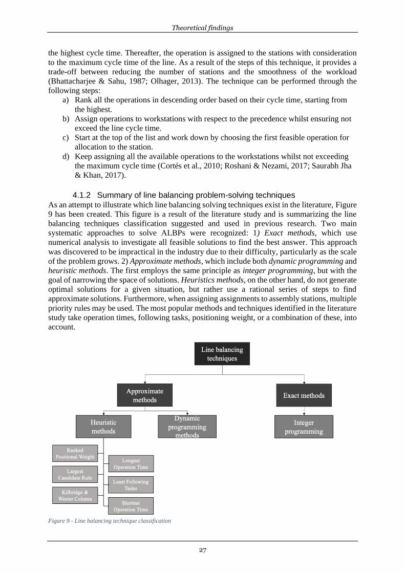
Theoretical findings
27
the highest cycle time. Thereafter, the operation is assigned to the stations with consideration
to the maximum cycle time of the line. As a result of the steps of this technique, it provides a
trade-off between reducing the number of stations and the smoothness of the workload
(Bhattacharjee & Sahu, 1987; Olhager, 2013). The technique can be performed through the
following steps:
a) Rank all the operations in descending order based on their cycle time, starting from
the highest.
b) Assign operations to workstations with respect to the precedence whilst ensuring not
exceed the line cycle time.
c) Start at the top of the list and work down by choosing the first feasible operation for
allocation to the station.
d) Keep assigning all the available operations to the workstations whilst not exceeding
the maximum cycle time (Cortés et al., 2010; Roshani & Nezami, 2017; Saurabh Jha
& Khan, 2017).
4.1.2 Summary of line balancing problem-solving techniques As an attempt to illustrate which line balancing solving techniques exist in the literature, Figure
9 has been created. This figure is a result of the literature study and is summarizing the line
balancing techniques classification suggested and used in previous research. Two main
systematic approaches to solve ALBPs were recognized: 1) Exact methods, which use
numerical analysis to investigate all feasible solutions to find the best answer. This approach
was discovered to be impractical in the industry due to their difficulty, particularly as the scale
of the problem grows. 2) Approximate methods, which include both dynamic programming and
heuristic methods. The first employs the same principle as integer programming, but with the
goal of narrowing the space of solutions. Heuristics methods, on the other hand, do not generate
optimal solutions for a given situation, but rather use a rational series of steps to find
approximate solutions. Furthermore, when assigning assignments to assembly stations, multiple
priority rules may be used. The most popular methods and techniques identified in the literature
study take operation times, following tasks, positioning weight, or a combination of these, into
account.
Figure 9 - Line balancing technique classification
Theoretical findings
28
4.2 RQ2 – Which investment costs can be considered vital for new assembly lines as a consequence from new product introductions?
The results of the literature study focusing on investment costs indicate that assembly line
investment costs are an important factor in a company's long-term economic performance.
However, the literature review also shows that among researchers, there is no well-established
methodology for estimating assembly line investment costs. The majority of researchers are
focusing on developing ways of predicting investments, such as Net present value (NPV) and
life-cycle costing (LCC). One of these researches is Tosatti’s (2006), who is presenting a
methodology for lifecycle design of production systems. In their research, costs are divided into
three categories; investment costs, fixed costs, and variable costs. The investment costs are
covering installations and the production system configuration. The fixed costs are, for instance,
related overhead and space rent costs. Lastly, variable costs are covering maintenance and
energy, i.e. costs dependent on the demand (Tosatti, 2006).
Seldom are researchers focusing on characterising and labelling the actual inputs of these
investments. For instance, Bond & Jenkinson (1996) argue that investments are two-folded and
comprise of intangible capital, frequently termed human capital, which includes skills and
education. The other perspective of investments regard fixed capital (Bond & Jenkinson, 1996).
Nevertheless, they do not specify the characteristics further. However, a few papers present
detailed assembly line investment costs categorization. Michalos et al. (2012) developed a
sophisticated method for developing and evaluating assembly line alternatives, which
incorporates the decision needed to be taken when designing an assembly line. In their research,
the investment costs are calculated as the total cost for acquiring and installing resources, e.g.
machines and tools, needed in the production.
Similarly, Padrón et al. (2009) is presenting a methodology for cost-oriented assembly line
balancing problems. Based on their previous research and consulting experience, Padrón et al.
(2009) divided investment costs, specifically for highly manual assembly lines, into two main
categories; short-term operating costs and capital investment costs. Short-term operating costs
cover employee wages and floor space costs. The latter, i.e. floor space costs, include rent and
complementary utilities. On the other hand, fixed capital investment costs can be divided into
two categories; task-related investment costs and workstation capital investment costs. The
former is related to costs required due to the task’s essence. Hence, they are necessary for
production to circumvent. These investments include costs related to the purchase of machines,
fixtures, equipment, and tools. Contrary, the workstation capital investment costs are associated
with standard equipment required at each workstation. These incorporate e.g. chairs,
workbenches, and mats (Padrón et al., 2009).
Regarding previous research conducted particularly on investment costs connected to
reconfigurable production, the literature study identified the works of Delorme et al. (2016) and
Sievers et al. (2017). The former, i.e. Delorme et al. (2016), defined the production line costs
in a reconfigurable transfer line as the cost per workstation and cost per CNC machine.
Contrary, Sievers et al. (2017) applied a modular production site design, where they considered
the fixed capital investment a key component in decision making. This key figure consisted of
material cost, plant construction and overhead costs. The former two categories are not
specified further, whilst the latter includes engineering and uncertainties costs (Sievers et al.,
2017).
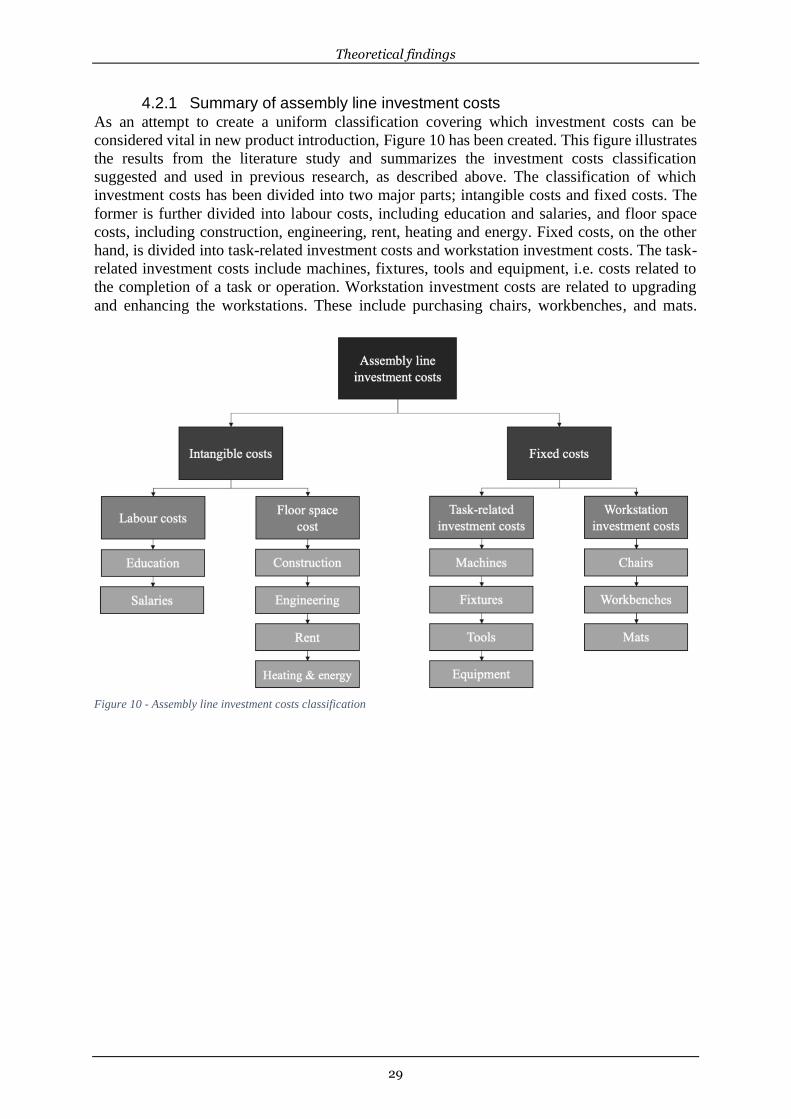
Theoretical findings
29
4.2.1 Summary of assembly line investment costs As an attempt to create a uniform classification covering which investment costs can be
considered vital in new product introduction, Figure 10 has been created. This figure illustrates
the results from the literature study and summarizes the investment costs classification
suggested and used in previous research, as described above. The classification of which
investment costs has been divided into two major parts; intangible costs and fixed costs. The
former is further divided into labour costs, including education and salaries, and floor space
costs, including construction, engineering, rent, heating and energy. Fixed costs, on the other
hand, is divided into task-related investment costs and workstation investment costs. The task-
related investment costs include machines, fixtures, tools and equipment, i.e. costs related to
the completion of a task or operation. Workstation investment costs are related to upgrading
and enhancing the workstations. These include purchasing chairs, workbenches, and mats.
Figure 10 - Assembly line investment costs classification
Theoretical findings
30
4.3 RQ 4 – To what extent can criteria in the RMS theory be linked with the attributes of the designed decision-making tool to support its applicability?
The literature study identified a correlation between RMS and mixed-model assembly line
balancing as both of these are handling the dilemma of efficiently producing a variety of product
variants in the same production system. Because while the earlier model for assembly lines
developed by Henry Ford used for mass production for one product. Mixed-model assembly
lines aim to produce various products within the same product family (Baybars, 1986; Shtub &
Dar-El, 1989). A standard mixed-model line balancing problem intends to define the need to
meet a specific performance objective. When addressing a balancing problem, several
considerations are taken into consideration based on given data and the objective of balancing.
These considerations may include one or more of the following: a given number of products,
operations associated with each product, task precedence relations within the line, takt times,
product demands, task times, and if the assembly line is equipped with buffers between stations
(Becker & Scholl, 2006; Chakravarty & Shtub, 1985; Erel & Gökçen, 1999).
Lohse (2006) linked the responsiveness of assembly lines and the variation of production
capacity in highly customized products, such a dynamic environment generates a need for
layouts, processes, and workers that support activities in response to production needs. Several
researchers have heightened the link between the mixed assembly line and reconfigurability
enablers. Koren & Shpitalni (2010) stated three reconfigurability characteristics associated with
reconfigurable assembly lines: customization, scalability, and convertibility. Customization
relates to the assembly systems ability to assemble all the products in the product family;
scalability ensures the system to increase productivity to meet the changing demand and
convertibility enables the assembly line to switch between assembling one product to another
within the product family in a rapid manner (Koren & Shpitalni, 2010; Youssef & Elmaraghy,
2006). Another key aspect of a reconfigurable assembly system is a modular conveyor system
which can be reconfigured to accommodate a variety of components according to the product
being assembled (Koren & Shpitalni, 2010).
The model of introducing a new product to the production system for the mixed-model
suggested by Fujimoto & Clark (1991) illustrates the new product is scaling up through time.
That is associated with increasing the production rate (Scalability); hence product introducing
models usually start with pilot production and scalability. However, by applying early changes
to products and production systems, it is expected to increase the production rate to achieve the
market target, a critical RMS aspect (Bellgran & Säfsten, 2009). Ulrich & Eppinger (2016)
illustrated the relation between new products and production at pre-production as a challenging
stage to fulfil quality and speed requirements. Both two requirements are connected to
Diagnosability and Flexibility, respectively.
Moreover, the production system must identify the root cause of product and process quality
issues during ramp-up to rectify them as early as possible to avoid the cost of late changes. The
smooth transition between the old and the new product with limited setup time or even without
setup time is in line with what Koren (1999) described as assembly line Convertibility. To sum
up, the literature study results provided insights into the correlation between RMS
characteristics and mixed-model assembly line balancing. It also indicated that in order to
establish an adequate way of evaluating RMS against mixed-model assembly line balancing,
and thus also the decision-making tool, the RMS characteristics need further explanation. The
literature study found the previous research by Rösiö et al. (2019) which covers a breakdown
of the RMS characteristics into detailed sub-characteristics as an approachable solution to this.
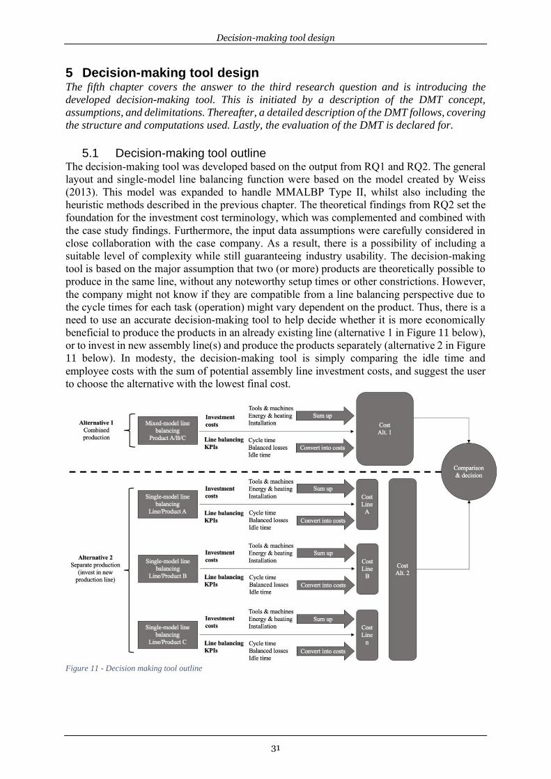
Decision-making tool design
31
5 Decision-making tool design The fifth chapter covers the answer to the third research question and is introducing the
developed decision-making tool. This is initiated by a description of the DMT concept,
assumptions, and delimitations. Thereafter, a detailed description of the DMT follows, covering
the structure and computations used. Lastly, the evaluation of the DMT is declared for.
5.1 Decision-making tool outline The decision-making tool was developed based on the output from RQ1 and RQ2. The general
layout and single-model line balancing function were based on the model created by Weiss
(2013). This model was expanded to handle MMALBP Type II, whilst also including the
heuristic methods described in the previous chapter. The theoretical findings from RQ2 set the
foundation for the investment cost terminology, which was complemented and combined with
the case study findings. Furthermore, the input data assumptions were carefully considered in
close collaboration with the case company. As a result, there is a possibility of including a
suitable level of complexity while still guaranteeing industry usability. The decision-making
tool is based on the major assumption that two (or more) products are theoretically possible to
produce in the same line, without any noteworthy setup times or other constrictions. However,
the company might not know if they are compatible from a line balancing perspective due to
the cycle times for each task (operation) might vary dependent on the product. Thus, there is a
need to use an accurate decision-making tool to help decide whether it is more economically
beneficial to produce the products in an already existing line (alternative 1 in Figure 11 below),
or to invest in new assembly line(s) and produce the products separately (alternative 2 in Figure
11 below). In modesty, the decision-making tool is simply comparing the idle time and
employee costs with the sum of potential assembly line investment costs, and suggest the user
to choose the alternative with the lowest final cost.
Figure 11 - Decision making tool outline
Decision-making tool design
32
Since most existing decision-making tools, and in particular existing line balancing tools (e.g.
Weiss, 2013), are either too complex to apply in a wider industry setting, or too limited
regarding adaption to the focal company, the DMT has been designed with reconfigurability in
mind. For instance, the reconfiguration of investment costs, whereas it is possible to either
include more cost categories if the user requires a more detailed result, or simply alter the
suggested categories to include the case relevant costs. These alternatives provide the user with
the possibility of changing the DMT in accordance with their company. Theoretically, the
DMT’s ability for scalability generates the possibility to test an unlimited number of products,
as highlighted in Figure 11 above. However, as informed by the case study respondent, in most
situations, companies are solely interested in testing whether a single new product is viable for
production in the existing line. This as product development frequently only occurs one at a
time. Therefore, the decision-making tool is solely structured to handle three products, whereas
two are new products. In the case where several products are already produced in the existing
line, and the goal is to determine whether it is possible to produce another product in the same
line, the authors suggest to pre-calculate the combined task times for the products produced in
the separate line.
Once the user has inserted the necessary inputs, the DMT automatically conducts both mixed-
model assembly line balancing and single-model assembly line balancing for all products. The
latter is achieved by using four different priority rules. The user then can select either select the
most line-efficient option as suggested by the DMT, or another priority rule if recognized as
being a better fit for the company. The mixed-model line balancing is using the priority rule
Longest Operation Time, however, the cycle time can be calculated in different ways. This
decision-making tool is conducting line balancing based on two ways: Max task time and
Weighted average task time. Based on, for instance, the company's product variety, the user has
the possibility to choose which task time fits their unique production setup.
Apart from the aforementioned assumptions, the decision-making tool is designed based on the
following assumptions:
• Task times are calculated beforehand by the user.
• No setup time is required when producing several product variants in the same line.
• Task times are including times for walking, moving products, and preparing the next
task.
• All parameters in the DMT are assumed to be deterministic.
• Task times are fixed, unless changed by the user.
• There is not a fixed set of stations, this is calculated by the decision-making tool.
• The total time of a task cannot exceed the required takt time. If a task is exceeding the
required takt time, the user must divide the task into two or more tasks in order for the
tool perform the line balancing.
• The assembly lines tested in the decision-making tool is constructed as serial lines, not
as U-shaped lines.
• The input parameters are correct, for instance, the predecessors must follow a logic
and true diagram.
• Each station needs exactly one worker.
• Fixed costs are based on the entire investment costs on, i.e. no depreciations are
calculated in the DMT. If depreciation should be included, the user must take this into
consideration when inserting input values.
• No production order sequencing is taken into consideration in the DMT. Instead,
products are calculated based on the overall production capacity on a yearly basis.
Decision-making tool design
33
• The product quality does not change when producing the new product(s) in either
separate or combines assembly lines.
• In the Monte Carlo simulation, the DMT operates on the basis that the outputs are
normally distributed.
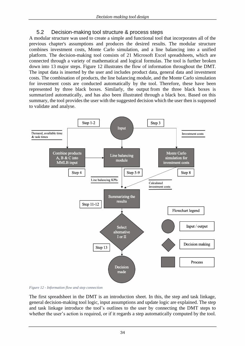
Decision-making tool design
34
5.2 Decision-making tool structure & process steps A modular structure was used to create a simple and functional tool that incorporates all of the
previous chapter's assumptions and produces the desired results. The modular structure
combines investment costs, Monte Carlo simulation, and a line balancing into a unified
platform. The decision-making tool consists of 21 Microsoft Excel spreadsheets, which are
connected through a variety of mathematical and logical formulas. The tool is further broken
down into 13 major steps. Figure 12 illustrates the flow of information throughout the DMT.
The input data is inserted by the user and includes product data, general data and investment
costs. The combination of products, the line balancing module, and the Monte Carlo simulation
for investment costs are conducted automatically by the tool. Therefore, these have been
represented by three black boxes. Similarly, the output from the three black boxes is
summarized automatically, and has also been illustrated through a black box. Based on this
summary, the tool provides the user with the suggested decision which the user then is supposed
to validate and analyse.
Figure 12 - Information flow and step connection
The first spreadsheet in the DMT is an introduction sheet. In this, the step and task linkage,
general decision-making tool logic, input assumptions and update logic are explained. The step
and task linkage introduce the tool’s outlines to the user by connecting the DMT steps to
whether the user’s action is required, or if it regards a step automatically computed by the tool.
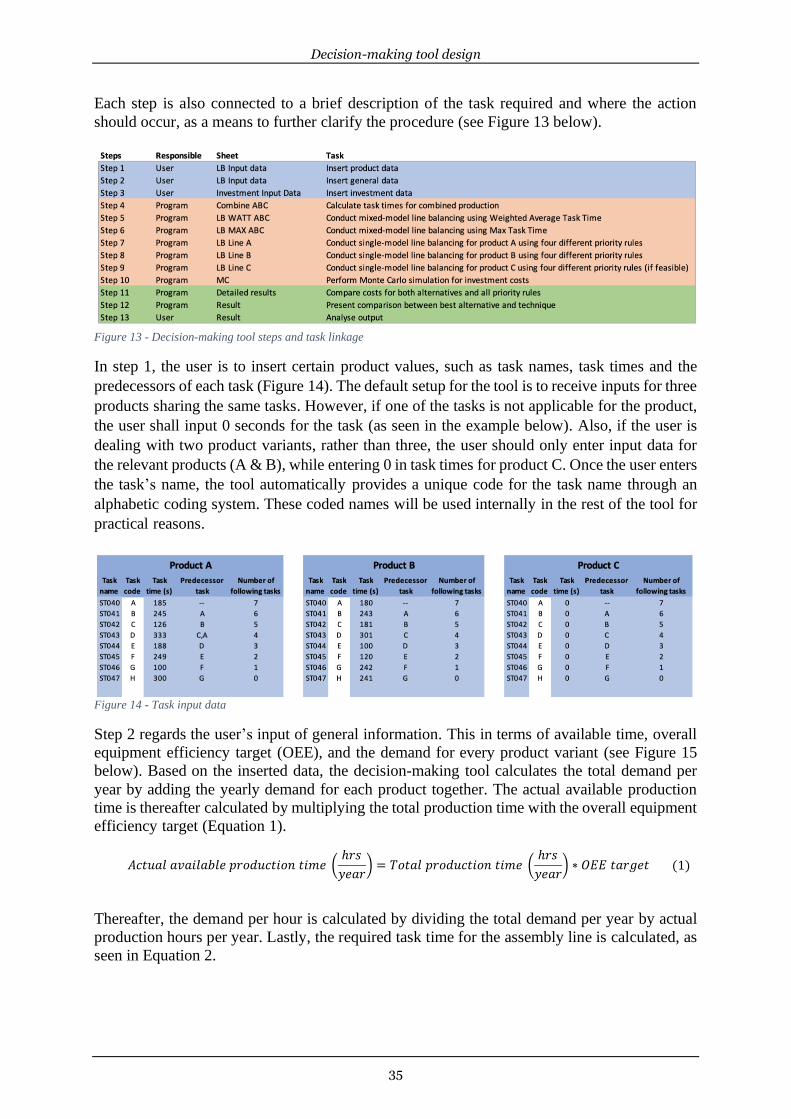
Decision-making tool design
35
Each step is also connected to a brief description of the task required and where the action
should occur, as a means to further clarify the procedure (see Figure 13 below).
Figure 13 - Decision-making tool steps and task linkage
In step 1, the user is to insert certain product values, such as task names, task times and the
predecessors of each task (Figure 14). The default setup for the tool is to receive inputs for three
products sharing the same tasks. However, if one of the tasks is not applicable for the product,
the user shall input 0 seconds for the task (as seen in the example below). Also, if the user is
dealing with two product variants, rather than three, the user should only enter input data for
the relevant products (A & B), while entering 0 in task times for product C. Once the user enters
the task’s name, the tool automatically provides a unique code for the task name through an
alphabetic coding system. These coded names will be used internally in the rest of the tool for
practical reasons.
Figure 14 - Task input data
Step 2 regards the user’s input of general information. This in terms of available time, overall
equipment efficiency target (OEE), and the demand for every product variant (see Figure 15
below). Based on the inserted data, the decision-making tool calculates the total demand per
year by adding the yearly demand for each product together. The actual available production
time is thereafter calculated by multiplying the total production time with the overall equipment
efficiency target (Equation 1).
𝐴𝑐𝑡𝑢𝑎𝑙 𝑎𝑣𝑎𝑖𝑙𝑎𝑏𝑙𝑒 𝑝𝑟𝑜𝑑𝑢𝑐𝑡𝑖𝑜𝑛 𝑡𝑖𝑚𝑒 (
ℎ𝑟𝑠
𝑦𝑒𝑎𝑟) = 𝑇𝑜𝑡𝑎𝑙 𝑝𝑟𝑜𝑑𝑢𝑐𝑡𝑖𝑜𝑛 𝑡𝑖𝑚𝑒 (
ℎ𝑟𝑠
𝑦𝑒𝑎𝑟) ∗ 𝑂𝐸𝐸 𝑡𝑎𝑟𝑔𝑒𝑡 (1)
Thereafter, the demand per hour is calculated by dividing the total demand per year by actual
production hours per year. Lastly, the required task time for the assembly line is calculated, as
seen in Equation 2.
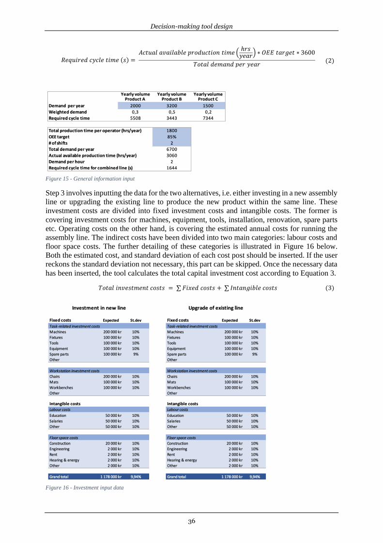
Decision-making tool design
36
𝑅𝑒𝑞𝑢𝑖𝑟𝑒𝑑 𝑐𝑦𝑐𝑙𝑒 𝑡𝑖𝑚𝑒 (𝑠) = 𝐴𝑐𝑡𝑢𝑎𝑙 𝑎𝑣𝑎𝑖𝑙𝑎𝑏𝑙𝑒 𝑝𝑟𝑜𝑑𝑢𝑐𝑡𝑖𝑜𝑛 𝑡𝑖𝑚𝑒 (
ℎ𝑟𝑠𝑦𝑒𝑎𝑟) ∗ 𝑂𝐸𝐸 𝑡𝑎𝑟𝑔𝑒𝑡 ∗ 3600
𝑇𝑜𝑡𝑎𝑙 𝑑𝑒𝑚𝑎𝑛𝑑 𝑝𝑒𝑟 𝑦𝑒𝑎𝑟
(2)
Figure 15 - General information input
Step 3 involves inputting the data for the two alternatives, i.e. either investing in a new assembly
line or upgrading the existing line to produce the new product within the same line. These
investment costs are divided into fixed investment costs and intangible costs. The former is
covering investment costs for machines, equipment, tools, installation, renovation, spare parts
etc. Operating costs on the other hand, is covering the estimated annual costs for running the
assembly line. The indirect costs have been divided into two main categories: labour costs and
floor space costs. The further detailing of these categories is illustrated in Figure 16 below.
Both the estimated cost, and standard deviation of each cost post should be inserted. If the user
reckons the standard deviation not necessary, this part can be skipped. Once the necessary data
has been inserted, the tool calculates the total capital investment cost according to Equation 3.
𝑇𝑜𝑡𝑎𝑙 𝑖𝑛𝑣𝑒𝑠𝑡𝑚𝑒𝑛𝑡 𝑐𝑜𝑠𝑡𝑠 = ∑ 𝐹𝑖𝑥𝑒𝑑 𝑐𝑜𝑠𝑡𝑠 + ∑ 𝐼𝑛𝑡𝑎𝑛𝑔𝑖𝑏𝑙𝑒 𝑐𝑜𝑠𝑡𝑠 (3)
Figure 16 - Investment input data
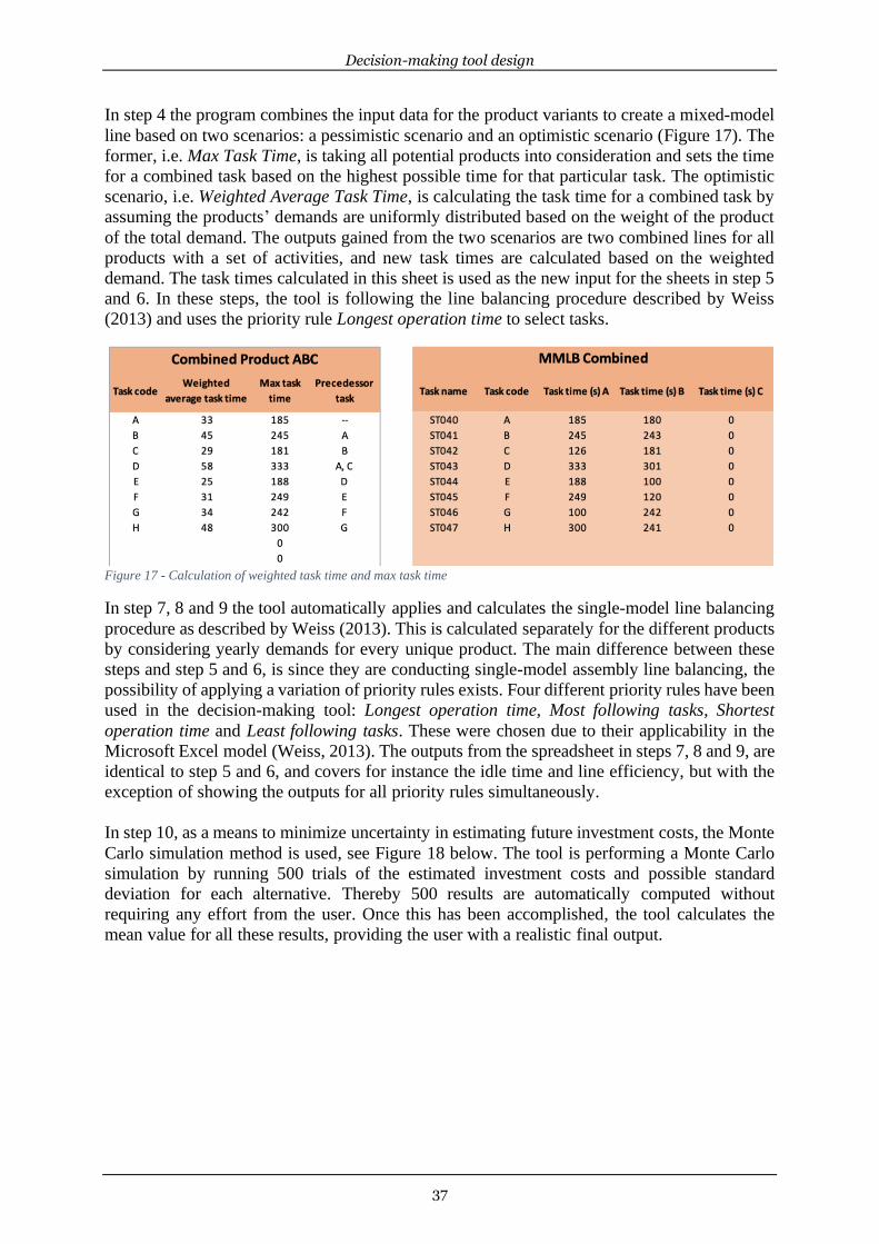
Decision-making tool design
37
In step 4 the program combines the input data for the product variants to create a mixed-model
line based on two scenarios: a pessimistic scenario and an optimistic scenario (Figure 17). The
former, i.e. Max Task Time, is taking all potential products into consideration and sets the time
for a combined task based on the highest possible time for that particular task. The optimistic
scenario, i.e. Weighted Average Task Time, is calculating the task time for a combined task by
assuming the products’ demands are uniformly distributed based on the weight of the product
of the total demand. The outputs gained from the two scenarios are two combined lines for all
products with a set of activities, and new task times are calculated based on the weighted
demand. The task times calculated in this sheet is used as the new input for the sheets in step 5
and 6. In these steps, the tool is following the line balancing procedure described by Weiss
(2013) and uses the priority rule Longest operation time to select tasks.
Figure 17 - Calculation of weighted task time and max task time
In step 7, 8 and 9 the tool automatically applies and calculates the single-model line balancing
procedure as described by Weiss (2013). This is calculated separately for the different products
by considering yearly demands for every unique product. The main difference between these
steps and step 5 and 6, is since they are conducting single-model assembly line balancing, the
possibility of applying a variation of priority rules exists. Four different priority rules have been
used in the decision-making tool: Longest operation time, Most following tasks, Shortest
operation time and Least following tasks. These were chosen due to their applicability in the
Microsoft Excel model (Weiss, 2013). The outputs from the spreadsheet in steps 7, 8 and 9, are
identical to step 5 and 6, and covers for instance the idle time and line efficiency, but with the
exception of showing the outputs for all priority rules simultaneously.
In step 10, as a means to minimize uncertainty in estimating future investment costs, the Monte
Carlo simulation method is used, see Figure 18 below. The tool is performing a Monte Carlo
simulation by running 500 trials of the estimated investment costs and possible standard
deviation for each alternative. Thereby 500 results are automatically computed without
requiring any effort from the user. Once this has been accomplished, the tool calculates the
mean value for all these results, providing the user with a realistic final output.

Decision-making tool design
38
Figure 18 - Monte Carlo simulation
In step 11 the decision-making tool is summarizing the detailed result for all previous
calculations, including the line balancing parameters for the two alternatives. Also, the
spreadsheet illustrates the task allocation for each station through colour coding. Furthermore,
the comparison between the two alternatives is highlighted through figures and colour coding.
This spreadsheet is intended mainly for users who desire a deeper insight into the outputs of the
tool. In step 12, the decision-making tool uses the exact data for visualizing and summarizing
the outputs for the two alternatives. The tool is converting the line balancing KPIs into costs
and is thus able to compare these with the investment costs. These are then compared, and a
final decision based on the lowest cost is suggested (Figure 19). In the final step, i.e. step 13,
the user shall analyze the result in order to completely understand the impact of the decision on
the company.
Figure 19 - Final result display
Decision-making tool design
39
5.3 Evaluation of the decision-making tool During the focus group occasion, the feedback gained underlined the case company’s necessity
of using the DMT for two primary reasons. Firstly, the participants indicated that the level of
uncertainty is frequently high during the early phases of new product development, hence the
need to make fact-based decisions is evident. Secondly, in line with the case company’s vision
of transitioning towards RMS, the decisions regarding how and where to produce a new product
will increase in frequency. Therefore, a structured and fact-based procedure needs to be
established in order to support this transition. The participants pointed out that the developed
DMT will indeed help in facilitating these decisions, and thus also take one step in the process
of moving towards RMS. Furthermore, the output of the DMT was recognized as being a
sufficient decision to continue the next step in the product development process. Because, the
decision regarding whether the new product(s) should be produced in an already existing
assembly line, or to invest in a new assembly line has been taken, will be forwarded to
production engineers. These employees will then consider it when designing and purchasing
the necessary equipment for the new setup.
The participants also found the DMT to be similar to the tools they are using in, for instance,
production planning and financial estimations. Establishing a similarity and coherence between
new and old tools was identified as an important factor since it reduces the time required for
users to understand the tool. However, it was declared that some parts in the DMT required
rephrasing in order to match the terminology used in other tools. On this topic, the participants
also approved the choice to create the DMT in Microsoft Excel. The approval was based on the
argument that the case company has other Microsoft Excel tools for scheduling and financing
functions which make new users instantly familiar with the DMT and reduces the effort
required for training new users. Likewise, due to the existing integrability between the DMT
and the case company’s other tools, the participants pointed towards the future possibility of
directly connecting several tools in order to further streamline the product development process.
Moreover, the input data required for the DMT to conduct the line balancing module was
recognized as easily being gathered from the production software AVIX, which the case
company frequently uses. The participants also provided insights into how historical data used
to estimate the time required to do every move in the assembly activities can be used an input
for the DMT. Likewise, the participants found the level of complexity in investment costs to be
at a satisfactory level. Because, using NPV and LCC was recognized as being far too detailed
and complicated to implement during the stage when using the DMT. The investment costs
were found to easily being gathered through rough estimation, which is already performed in
the case company’s current procedure. The Monte Carlo simulation was received with praise
as it facilitates the reduction of investment costs estimation uncertainty, whilst not requiring
any significant effort from the user.
During the focus group, it was also confirmed that there are two levels of users who will operate
the tool: users on a technical level and on a managerial level. The former regards user who can
edit the tool and have a deep understanding of intermediate steps. The latter includes users who
are solely interested in the final result, and are therefore not interested in how the DMT has
reached the decision. Due to the existence of these user levels, the participants in the focus
group found it necessary to provide enough information on each Microsoft Excel sheet so users
on the technical level will easily understand the process and logic in the DMT. Regarding this,
it was also recommended that users could have different levels of access to the tool since some
worksheets will be hidden. This restriction reflects the tool’s flexibility to answer questions on
both managerial and technical levels.
Analysis & discussion
40
6 Analysis & discussion
The sixth chapter beings with an analysis and discussions of the research questions. Thereafter
the methods used in the thesis are discussed.
6.1 Analysis and discussion of findings The discussion of findings has been divided into four parts, each covering the analysis and
discussion for a unique research question.
RQ 1 - Which line balancing problem-solving techniques exist in the literature? The first research question was addressed by a literature review, and the basic assumptions of
assembly line balancing problems were established and categorized. A selection of the
identified line balancing problem-solving techniques was used to develop the decision-making
tool. These were selected based on usability and possible integration with Microsoft Excel
functions. Product diversity drives assembly line balancing problems categorization into two
types: single model assembly lines and mixed-model assembly lines. Conversely, ALBP is
classified based on the goals of line balancing; Type I problems consider an assembly line with
a set number of stations, with the goal of increasing production rate, while Type II problems
presume constant process times with the goal of increasing production capability by reducing
delay time (Erel & Sarin, 1998; Watanabe et al., 1995).
The result of the literature study also exposed an incoherent view on solving line balancing
problems. Many techniques have been developed throughout the years, which all vary in
complexity and usability. This might explain why the field of line balancing techniques is very
broad, and why new techniques are continuously being developed. Though, there is no approach
that fits for all types of problems, and newly developed techniques often seem to solely provide
solutions to a specific problem. This issue might partly derive from the unique situation
companies are in when entailing to conduct line balancing, and thus creating a generic technique
is incredibly difficult. This might be a reason why very simple heuristic solutions, such as RPW
and LCR, have lasted amongst theoreticians and are among the most commonly used techniques
in the industry.
Many approaches have been established to address both types of problems. To begin, integer
programming seeks exact solutions to problems by exploring all possible solutions, while
dynamic programming divides problems into sub-steps and excludes the space of investable
solutions. Both techniques were found to be complicated to apply in the industry, the algorithms
of solutions become quite complex when the number of stations increases. Heuristic approaches
were introduced to fulfill the limitations of these techniques. The heuristic approaches generate
approximate solutions based on common sense and logical sequence of applying the line
balancing assumptions and priority mechanisms. The three above-mentioned techniques have
the same goal in mind: minimizing balance delay and create a more uniform workload
distribution among stations in the line. Different dedicated software’s developed based on
these algorithms.
The literature review generated only four articles when searching with the combination of
"Reconfigurable manufacturing system" OR "RMS" AND "Mixed-model assembly line". This
limited number of articles indicates that the concept of reconfigurability is still ambiguous and
not as common in operations research academia. Additional case studies can reveal how
effective are those approaches in different industrial setups.

Analysis & discussion
41
The answer to RQ1 is summarized in Figure 9; line balancing strategies will differ depending
on the goal of the balancing, product variation within the line, or the level of accuracy needed.
Where an approximate solution with a high degree of applicability is required, heuristic
solutions are the most flexible. Moreover, as far as we know, no general solution has been
created to match the framework of RMS. The limited number of publications regarding mixed-
model assembly line balancing within RMS context makes it difficult to understand the
implications of different balancing techniques on the performance of RMS characteristics. It is
also important to remember that the limitation of both Exact and Approximate methods are
related to the accuracy and time efficiency of the calculations mainly. That means a future
production system with a low level of uncertainty and timely data exchange within the entire
industrial supply chain may not have to face the trade-offs between time-consuming
calculations and accurate line balancing results. Such a future production system may benefit
from the location in the spectrum of new industry 4.0 trends.
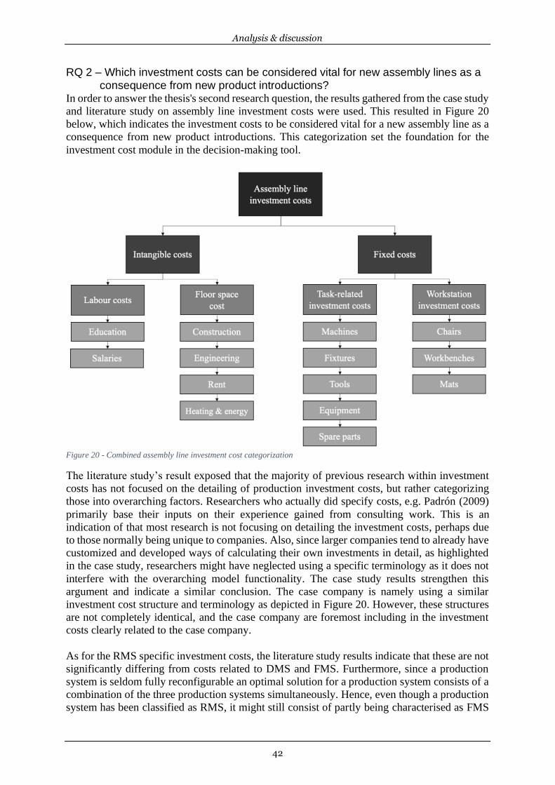
Analysis & discussion
42
RQ 2 – Which investment costs can be considered vital for new assembly lines as a consequence from new product introductions?
In order to answer the thesis's second research question, the results gathered from the case study
and literature study on assembly line investment costs were used. This resulted in Figure 20
below, which indicates the investment costs to be considered vital for a new assembly line as a
consequence from new product introductions. This categorization set the foundation for the
investment cost module in the decision-making tool.
Figure 20 - Combined assembly line investment cost categorization
The literature study’s result exposed that the majority of previous research within investment
costs has not focused on the detailing of production investment costs, but rather categorizing
those into overarching factors. Researchers who actually did specify costs, e.g. Padrón (2009)
primarily base their inputs on their experience gained from consulting work. This is an
indication of that most research is not focusing on detailing the investment costs, perhaps due
to those normally being unique to companies. Also, since larger companies tend to already have
customized and developed ways of calculating their own investments in detail, as highlighted
in the case study, researchers might have neglected using a specific terminology as it does not
interfere with the overarching model functionality. The case study results strengthen this
argument and indicate a similar conclusion. The case company is namely using a similar
investment cost structure and terminology as depicted in Figure 20. However, these structures
are not completely identical, and the case company are foremost including in the investment
costs clearly related to the case company.
As for the RMS specific investment costs, the literature study results indicate that these are not
significantly differing from costs related to DMS and FMS. Furthermore, since a production
system is seldom fully reconfigurable an optimal solution for a production system consists of a
combination of the three production systems simultaneously. Hence, even though a production
system has been classified as RMS, it might still consist of partly being characterised as FMS

Analysis & discussion
43
and DMS. This is correlating with the results gained from the case study. Because, the case
company has thus far not developed specific economic investment calculus nor made any
adjustment to the current structure in order to fit specifically for RMS. This lack of adjustment
might perhaps derive from the fact that the case company still having an overarching part of
their entire production facility as being characterised as FMS and DMS, not RMS. Or perhaps
due to the relative newness of RMS, and hence no established way of including the RMS
specific characteristics have yet been developed. Studying the sub-characteristics of RMS, as
described by Rösiö et al. (2019), it is also possible to relate the absence of RMS integration to
the investment cost terminology simply due to a lack of necessity. Because, the investment
costs covering for instance machines, tools and fixtures, which are a major part in the work of
Rösiö et al. (2019), are already included in the investment cost terminology, for instance in the
research by Padrón et al. (2009), Delorme et al. (2016) and Michalos et al. (2012). The
aforementioned investment costs are solely describing the costs on a principal level, not the
implications of those. Thereby the investment cost terminology might not require major updates
in order to realistically reflect RMS, at least not during the early stages of new product
development.
Even in research where NPV and LCC calculations are present, as in the works of Tosatti
(2006), the costs are simply examples of what to include under certain suggested investment
cost headings and not specified any further. Using an investment calculation such as NPV or
LCC would indeed increase the accuracy of the investment output. However, as NPV and LCC
are very detailed and complex investment calculations, primarily used when making specific
investment decisions, these can be reckoned as not suitable to use during the early stages of
new product development. Instead, following the procedure in the case company seems like a
more suitable option. Since, as shown in the case study results, the case company only
performed a rough investment cost estimation during the early stages of new product
development, whilst NPV was performed once making the actual investment decision.
To conclude, the results from the literature review and document study provided a new
categorization of which investment costs can be considered vital for a new assembly lines as a
consequence from new product introductions. However, even though these investment costs are
covering both a theoretical and empirical aspect, the usability can be recognized as being
limited. This since investment cost terminology is a particularly subjective area, where
companies tend to have their own specific way of structuring investment costs, as proven by
the vast irregularities which the literature study exposed. The suggested structure in this thesis
was found to be sufficient for the case company to utilize the decision-making tool, whilst also
being general enough to cover the possibility of other companies also using the decision-making
tool without recognizing the need to alter the investment cost terminology. On this topic, the
theoretical findings and document study findings exposed almost identical investment costs,
hence the figure previously illustrated in Figure 20 does not differ significantly from Figure 10
covering the theoretical findings. The focus of this report implied that the overarching
discussion should not regard which wording to use when describing the investment costs, but
rather ensure to cover all relevant costs for a new assembly line through collecting data from
both literature and document study. Similarly, since the output form RQ2 was used as an input
for developing the decision-making tool, solely covering all necessary investment costs should
suffice for providing an accurate result to the research question.
Analysis & discussion
44
RQ 3 – Can a decision-making tool be designed to evaluate new product introductions which considers both line balancing KPIs and investment costs in an assembly line?
In order to answer RQ3, the findings from RQ1 and RQ2 were used. These findings set the
foundation for the decision-making tool’s two black-box modules. The first module was
covering conducting single-model and mixed-model line balancing, while the second module
was related to investment costs. A tailored model was created based on the design guidelines
for spreadsheets developed by Caine and Robson (1993). Data was gathered through a single-
case study, including interviews with the supervisor from the case company, document studies
and a focus group. The latter aided in assessing market practices against the various theoretical
approaches. By using the aforementioned procedure, the new decision-making tool was
constructed based on Weiss’ (2013) model. Following that, in multiple iterations, mixed-model
assembly line balancing, investment costs, and Monte Carlo simulation were added to the
decision-making tool. This technique allowed for design agility and assisted in the correction
and tracing of errors within the spreadsheets. Finally, for validation and testing purposes, the
line balancing module solved examples from Groover (2016) and the results were compared
with the correct answers given by Groover (2016).
A review of the literature revealed multiple line balancing techniques. However, the model
developed by Weiss (2013) was found to be the most adequate to the constraints considered in
this research. Primarily since it deems priority rules and adopted a modular structure. By
creating the models based on an already existing model, the authors were able to focus on the
main purpose of this thesis, i.e. to create a decision-making tool specifically for RMS.
Nonetheless, the previous model had several drawbacks that needed to be addressed if it wanted
to adapt it to mixed-model assembly line balancing and RMS and ensure user-friendliness.
Because, the old model seemed to be working to solve a specific solution, but not generalizable
and usable in a wider industrial setting continuously. One of the identified drawbacks regards
for example modifying the model, which is a relatively difficult task in Weiss’ (2013) model.
Another downside of the former model is the naming of operations. If one of the names is part
of another activity name, the algorithm will generate an error because the task name is verified
using the offset function. Using a more sophisticated technique to conduct MMALB, for
instance through Integer programming would perhaps provide a slightly more accurate result,
but would simultaneously increase the tool’s complexity significantly. Hence solely changing
the combined task time using Max Task Time and Weighted Average Task Time, and thereafter
use the priority rule Longest operation time to select task order, facilitated an increased tool
usability.
Even though the model presented by Weiss (2013) was a valid starting point for developing the
new decision-making tool, the previous model was recognized as not being user-friendly when
it comes to adding new tasks. Because, tasks were needed to be added in between existing tasks,
and following edits at other sheets were required. In contrast, while in the DMT developed in
this thesis was developed in a way that the user easily can add more tasks, without affecting the
rest of the model. The maximum possible number of tasks in each assembly line in the DMT is
set to 50, with the option of using any number of operations less than the maximum. The
previous model put redundant effort on the users, for instance, task names were needed to be
changed into alphabetic manually. This makes the model sensitive letters case and may be a
source of model failures, which can make the tracing of tasks more difficult. In order to tackle
this issue, auto coding functions were added to the DMT. The auto coding was created to allow
the user to add the real names of the tasks and the tool would create internal alphabetic coding
for every task. This internal coding was then used throughout the computations. Another
Analysis & discussion
45
function added to the DMT was colour coding for stations. In the line balancing result
spreadsheet, every task assigned within the same stations has been highlighted with the same
colour. By adding this function, the user is able to easily identify which tasks have been
assigned to each station.
The development of the investment module faced not only minor implications of combining
theoretical findings and empirical data to create and find a solution which is both general, but
also fitting the relevant stage in the product development. The DMT was created to establish a
way to structure early investment calculations by using a combination of both theoretical
investment costs and the one identified in the document analysis and through interviews.
Several investment costs, without taking the depreciations into consideration, were used in the
DMT as direct inputs to minimize the model's complexity. However, the investment calculation
black box is designed to be flexible enough to enable the user to easily change the investment
costs terminology without disrupting any corresponding steps. Furthermore, in order to
decrease the uncertainty of estimating investment costs, the Monte Carlo simulation was added
to the DMT. By doing this, it was possible to reduce some of the uncertainty connected to
estimating investment costs at an early product development phase. However, this input has
been developed in a structure where the users themselves have the option to choose to
implement this procedure. Because if not, the user simply has to insert a value of 0 for the
standard deviation with the aim of neglect this during the simulation. The output will then only
consist of the summarized expected outcome for the investment cost posts. Hence, providing
the user with the option of adapting the usage of Monte Carlo simulation according to their
preferences might also enhance a broader usability.
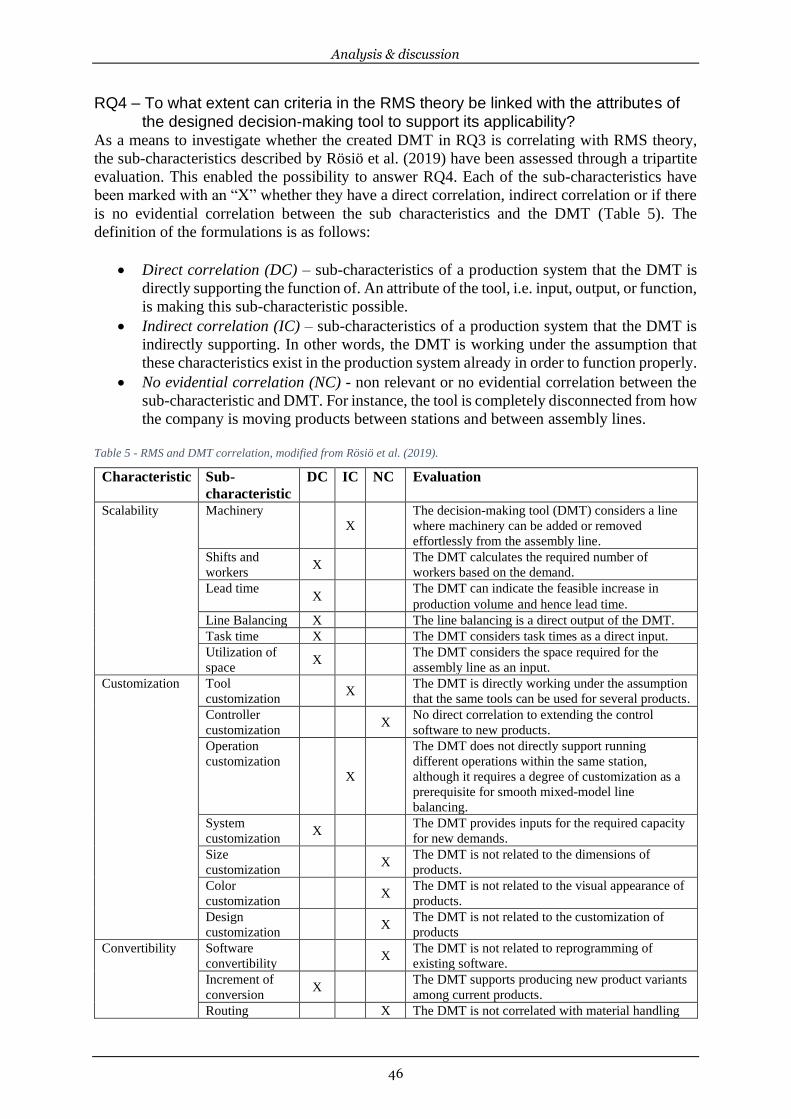
Analysis & discussion
46
RQ4 – To what extent can criteria in the RMS theory be linked with the attributes of the designed decision-making tool to support its applicability?
As a means to investigate whether the created DMT in RQ3 is correlating with RMS theory,
the sub-characteristics described by Rösiö et al. (2019) have been assessed through a tripartite
evaluation. This enabled the possibility to answer RQ4. Each of the sub-characteristics have
been marked with an “X” whether they have a direct correlation, indirect correlation or if there
is no evidential correlation between the sub characteristics and the DMT (Table 5). The
definition of the formulations is as follows:
• Direct correlation (DC) – sub-characteristics of a production system that the DMT is
directly supporting the function of. An attribute of the tool, i.e. input, output, or function,
is making this sub-characteristic possible.
• Indirect correlation (IC) – sub-characteristics of a production system that the DMT is
indirectly supporting. In other words, the DMT is working under the assumption that
these characteristics exist in the production system already in order to function properly.
• No evidential correlation (NC) - non relevant or no evidential correlation between the
sub-characteristic and DMT. For instance, the tool is completely disconnected from how
the company is moving products between stations and between assembly lines.
Table 5 - RMS and DMT correlation, modified from Rösiö et al. (2019).
Characteristic Sub-
characteristic
DC IC NC Evaluation
Scalability Machinery
X
The decision-making tool (DMT) considers a line
where machinery can be added or removed
effortlessly from the assembly line.
Shifts and
workers X
The DMT calculates the required number of
workers based on the demand.
Lead time X
The DMT can indicate the feasible increase in
production volume and hence lead time.
Line Balancing X The line balancing is a direct output of the DMT.
Task time X The DMT considers task times as a direct input.
Utilization of
space X
The DMT considers the space required for the
assembly line as an input.
Customization Tool
customization X
The DMT is directly working under the assumption
that the same tools can be used for several products.
Controller
customization X
No direct correlation to extending the control
software to new products.
Operation
customization
X
The DMT does not directly support running
different operations within the same station,
although it requires a degree of customization as a
prerequisite for smooth mixed-model line
balancing.
System
customization X
The DMT provides inputs for the required capacity
for new demands.
Size
customization X
The DMT is not related to the dimensions of
products.
Color
customization X
The DMT is not related to the visual appearance of
products.
Design
customization X
The DMT is not related to the customization of
products
Convertibility Software
convertibility X
The DMT is not related to reprogramming of
existing software.
Increment of
conversion X
The DMT supports producing new product variants
among current products.
Routing X The DMT is not correlated with material handling

Analysis & discussion
47
convertibility outside the assembly line.
Line routing
configurability X
The DMT supports parallel stations within the same
line.
Replicated
machines X
The DMT works in a setup where it is possible to
replicate machines to increase production capacity
Fixture
convertibility X
The DMT considers neglectable setup time for
fixtures, assuming that the setup of the assembly
line to the new variants setting is achieved
automatically.
Tool
convertibility X
The DMT considers neglectable setup time for
tools, assuming that the setup of the assembly line
to the new variants setting is achieved
automatically.
Multi-
directional X
The DMT solely focuses on operations, not other
activities between stations and between assembly
lines.
Asynchronous
motion X
The DMT solely focuses on operations, not other
activities between stations and between assembly
lines.
Level of
automation X
The DMT is not related to the system’s ability to
include a high level of automation.
Modularity Tool
modularity X
The DMT is working under the assumption that
tools are either modular or product variants share
the same tools.
Workstation
modularity X
The DMT is working under the assumption that
workstations are either modular or product variants
share the same workstations.
Fixture
modularity X
The DMT is working under the assumption that
fixtures are either modular or product variants share
the same fixtures.
Operation
sequence
X
The DMT’s main purpose is to investigate the
ability to produce two or more product variants in
the same line, and then structure operations
sequence to fit all variants within the same product
family.
Component
sharing
X
Due to that the DMT has been designed to cope
with single-model and mixed-model line balancing,
it is only working for products within the same
product family (otherwise, setup time would be
required to include).
Component
swapping X
The DMT does not depend on which components
the product variants consist of, but solely on the
operations required to produce those.
Cut to fit X
The DMT does not depend on which modules are
used in the product variants.
Bus modularity X
The DMT does not depend on which modules are
used in the product variants.
Integrability Tool
integrability X
The DMT is working under the assumption that
integration of new tools in existing machines is
possible.
Fixture
integrability* X
The DMT is operating on the assumption that
different fixtures will be integrated with existing
machines.
Control
software X
Software integrability is not affected nor affecting
the DMT.
Information
handling
integrability X
The DMT can easily be integrated with similar
tools within managerial and financial analysis, if
those are created in Microsoft Excel (or in other
compatible software).

Analysis & discussion
48
Diagnosability Poka yoke
X
The DMT does not affect, nor is affected by the
capability to detect the usage of correct tool and
components for the product variants.
Information
board X
The DMT is providing the user with information
regarding which production task sequence to
follow.
Traceability X
The DMT is not directly connected to any
traceability information or diagnosability tools.
Quality
assurance X
The DMT does not take quality changes into
consideration.
* Sub-characteristic added by authors of this thesis.
To illustrate the overarching connection between RMS characteristics and the decision-making
tool, the following table was created (Table 6). The direct connections are to be reckoned as
significant for the DMT, and thus their numerical value is worth significantly more than the
indirect correlations.
Table 6 - RMS characteristics and DMT correlation summary
Characteristic Direct
correlation
Indirect
correlation
No
correlation Scalability 5 1 -
Customization 1 2 4
Convertibility 2 3 5
Modularity 1 3 4
Integrability - 2 1
Diagnosability 1 - 3
Total 10 11 17
In order to further describe the evaluation between RMS sub-characteristics and the DMT, the
following paragraphs have been created.
Scalability, the evaluation showed a direct correlation with 5 out of 6 sub-characteristics within
scalability. These are primarily related to the system’s ability to adjust production capacity. For
instance, the line balancing module in the decision-making tool calculates the required number
of workers or stations based on the demand and available working time. This established a
direct correlation to the sub-characteristics line balancing, shift and workers, lead time and line
balancing. Furthermore, the investment perspective of the decision-making tool considers rent
of the area as a factor to calculate investment costs, which is related to the utilization of space.
Only a single sub-characteristic was classified as having an indirect correlation to the DMT,
this covered the possibility to add machines easily. This inherent ability of the production
system is a prerequisite in order to conduct line balancing, as otherwise the MMALB would
not be possible. Hence it was recognized as having an indirect correlation to the DMT.
Customization, the DMT did not indicate any strong overall connections to the RMS sub-
characteristics within customization. Primarily since there are no correlations between the DMT
and product features such as size, color, and design. Also, the DMT is not connected to control
customization and software that is used to control the production process. However, two sub-
characteristics were found to have indirect correlations with the DMT. One of these regards the
tool’s ability to arrange processes within the stations, i.e. tool customization. This was identified
as an indirect correlation since the mixed-model assembly line assumes that the same tools can
be used to produce different product variants. Therefore this is recognized as a major part of
the DMT’s assumption. The second sub-characteristic with an indirect correlation to the DMT
involves the operation customization required when running different processes within the same
Analysis & discussion
49
station. Lastly, the only direct correlation identified involves system customization. This since
the tool evaluates the decision of introducing a new product to the existing production system,
which is the core of this sub-characteristic.
Convertibility, only two sub-categories within convertibility were recognized as having a direct
connection with the tool. These regards incremental of conversion and line routing
configurability. The DMT was designed in order to test the capability of producing a new
product variant in an already existing production line which is a clear connection to the sub-
characteristic incremental of conversion. As for the line routing, since the DMT is supporting
parallel stations within the same assembly line, a direct connection was recognized.
Furthermore, the sub-characteristics fixture convertibility and tool convertibility were defined
as having an indirect correlation with the tool’s attributes. This indirect correlation was
identified since the basic assumption of the DMT is to neglect the setup time required when
changing between product variants. Furthermore, half of the sub-characteristics were classified
as having no evidential correlation to the DMT. This due to the fact that the DMT focuses on
an assembly line level and is not connected to the routing of AVGs or the programming of other
production software. Similarly, the sub-characteristics multidirectional and asynchronous
motion were identified as not relevant since the material handling equipment of the line is not
related to the DMT. Lastly, since the DMT works in a reconfigurable context without
considering the level of automation in the assembly line, this sub-characteristic was evaluated
as having no evidential correlation to the tool.
Modularity, in total three of the sub-characteristics were connected to having an indirect
correlation with the DMT. These regard tool, workstation, and fixture modularity. The
identified connection is that the DMT is working under the assumption that physical aspects of
a production system are modular, as it otherwise would not be possible to efficiently produce
product variants within the same assembly lines without extensive setup time. And since the
DMT does not take account for setup-time, these sub-characteristics fit under the indirect
correlation. The sub-characteristic operation sequence was the only part matched with a direct
correlation. This since the DMT’s main purpose is to investigate the ability to produce two or
more product variants in the same line, and then structure operations sequence to fit all variants
within the same product family. Lastly, four sub-characteristics within modularity were
identified as having no correlation with the DMT. These sub-characteristics were formulated
from a product development perspective, which is not related to the DMT since it solely focused
on production systems.
Integrability, two of the sub-characteristics within integrability were identified as having an
indirect correlation with the DMT. These sub-characteristics cover tool integrability and
information handling integrability. The former since the DMT is working under the assumption
that integration of new tools in existing machines is possible, otherwise a mixed-model
assembly line balancing procedure would not be possible. This would automatically result in
the requirement of purchasing a completely new assembly line, including tools and fixtures.
The latter sub-characteristic, i.e. information handling integrability, was recognized as having
an indirect correlation due to the DMT’s ability to easily be integrated with other Microsoft
Excel files. The integration can, for instance, regard tools within managerial and financial
analytics. The only sub-characteristic identified as neither being affected by nor affecting the
DMT was control software, which involves the capability to integrate already existing control
software into new tools, fixtures, and machines. The non-existent correlation to the DMT was
recognized since the control software is focusing on a technical level and not on a planning
level which the focal point in the DMT. Furthermore, the sub-characteristic fixture integrability
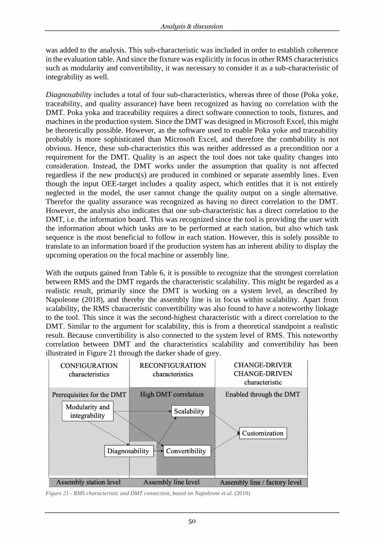
Analysis & discussion
50
was added to the analysis. This sub-characteristic was included in order to establish coherence
in the evaluation table. And since the fixture was explicitly in focus in other RMS characteristics
such as modularity and convertibility, it was necessary to consider it as a sub-characteristic of
integrability as well.
Diagnosability includes a total of four sub-characteristics, whereas three of those (Poka yoke,
traceability, and quality assurance) have been recognized as having no correlation with the
DMT. Poka yoka and traceability requires a direct software connection to tools, fixtures, and
machines in the production system. Since the DMT was designed in Microsoft Excel, this might
be theoretically possible. However, as the software used to enable Poka yoke and traceability
probably is more sophisticated than Microsoft Excel, and therefore the combability is not
obvious. Hence, these sub-characteristics this was neither addressed as a precondition nor a
requirement for the DMT. Quality is an aspect the tool does not take quality changes into
consideration. Instead, the DMT works under the assumption that quality is not affected
regardless if the new product(s) are produced in combined or separate assembly lines. Even
though the input OEE-target includes a quality aspect, which entitles that it is not entirely
neglected in the model, the user cannot change the quality output on a single alternative.
Therefor the quality assurance was recognized as having no direct correlation to the DMT.
However, the analysis also indicates that one sub-characteristic has a direct correlation to the
DMT, i.e. the information board. This was recognized since the tool is providing the user with
the information about which tasks are to be performed at each station, but also which task
sequence is the most beneficial to follow in each station. However, this is solely possible to
translate to an information board if the production system has an inherent ability to display the
upcoming operation on the focal machine or assembly line.
With the outputs gained from Table 6, it is possible to recognize that the strongest correlation
between RMS and the DMT regards the characteristic scalability. This might be regarded as a
realistic result, primarily since the DMT is working on a system level, as described by
Napoleone (2018), and thereby the assembly line is in focus within scalability. Apart from
scalability, the RMS characteristic convertibility was also found to have a noteworthy linkage
to the tool. This since it was the second-highest characteristic with a direct correlation to the
DMT. Similar to the argument for scalability, this is from a theoretical standpoint a realistic
result. Because convertibility is also connected to the system level of RMS. This noteworthy
correlation between DMT and the characteristics scalability and convertibility has been
illustrated in Figure 21 through the darker shade of grey.
Figure 21 - RMS characteristic and DMT connection, based on Napoleone et al. (2018)

Analysis & discussion
51
Furthermore, the characteristics modularity, integrability and diagnosability were found to a
fairly low overarching correlation with the DMT. This since they only had either zero or one
sub-characteristic with a direct correlation to the DMT. Given the fact that those characteristics
are, according to Napoleone (2018), within the workstation level, the fact that those are more
related to indirect correlation can be regarded as reasonable. Because, these characteristics are
a prerequisite for the scalability and convertibility, hence they are also a prerequisite for the
DMT. However, having scalability and convertibility within the system level can also facilitate
developing customisation within the system/factory level, which is indicated by the fairly non-
existent connection between the DMT and this particular characteristic, i.e. customization.
In summary, the DMT is working in a setup where modularity and integrability are within the
workstation level, i.e. machines and cells, hence they are prerequisites for the DMT to work,
rather than input, outputs, or attributes of the DMT. Neglection of these characteristics should
occur, because they support the scalability and convertibility within the system level, i.e. the
assembly lines, which are the characteristics directly correlated to the DMT. Similarly,
scalability and convertibility in a system-level is a prerequisite for having customization at the
factory level. This indicates that the model is supporting the customization at the assembly
line/factory level, which in turn affects the company’s overarching ability to deal with
fluctuations in the demands and an increased product introduction rate. Through this support,
the DMT can be recognized as a way to facilitate companies’ transition towards reconfigurable
manufacturing systems.
Even though the analysis between the DMT and RMS sub-characteristics can be recognized as
a valid evaluation method, it has some downsides and limitations. For instance, the amount and
formulation of the sub-characteristics presented by Rösiö et al. (2019) might have a major
impact when measuring the sum of correlations. Thereby, any potential imbalance amongst
sub-characteristics will affect the measuring. These imbalances can, for instance, regard a
higher amount of sub-characteristics related to a certain RMS characteristic, causing a probable
higher numerical value. Therefore, the results should not be regarded as a numerical result, but
rather as a way to establish a connection between RMS and the DMT on a principal level. Issues
regarding unbalanced sub-characteristics were recognized. For instance, several sub-
characteristics are focusing on AGVs. But since the DMT is solely limiting to assembly lines,
and not the surrounding production system, the numerical result is highly affected for the entire
characteristic. Similarly, several sub-characteristics such as component swapping, cut to fit and
bus modularity were more closely related to product configuration rather than production
systems. This created a similar effect on the numerical result as the aforementioned issue. These
issues might have caused limitations to the conclusions drawn in this thesis, however the results
can still be recognized as valid due to the theoretical coherence found in the analysis.

Analysis & discussion
52
6.2 Discussion of method This thesis was carried out with a structure primarily focusing on exploring and explaining.
These attributes correspond to a qualitative research approach (Leedy et al., 2019). The
qualitative approach is namely characterized as having flexible guidelines which were
necessary since the outcomes were not predetermined, but instead explorative. Choosing this
approach helped to answer research questions in a field where a unanimous theoretical
foundation was lacking. Literature studies were carried out as a means to answer the first and
second research question, whilst also setting the theoretical foundation for answering the fourth
research question. The literature studies followed a modified five step procedure, originally
developed by Booth et al. (2016). Extensive literature studies were conducted in three areas:
RMS, line balancing and assembly line investment costs. These covered broad areas, as a means
to investigate all possible options for developing and evaluating the decision-making tool.
Following a structured literature study procedure in several fields was crucial given that the
study’s purpose was partly explorative and focused the combination of several theoretical fields
which have not been studied simultaneously before. However, covering broad theoretical areas
also brough implications. For instance, due to line balancing being a significantly broad area
with a substantial amount of potential techniques and algorithms, there was a possibility that
not all of these were identified in the literature study. As a means to minimize this issue, several
searches within each literature study were conducted.
In order to develop the decision-making tool, and thereby create the possibility to answer the
third and fourth research question, a single case study was carried out. However, as the case
study was conducted in an industry specific context, transferability was restricted. To battle this
issue, the decision-making tool was thoroughly explained in order to grant readers the
possibility of deciding whether it can be applied in their area, i.e. thick description (Lincoln &
Guba, 1985). Furthermore, to increase credibility, data triangulation was implemented in the
case study. This included document studies, interviews and focus group. The document studies
were carried out by the focal company sending the documents electronically, which were then
studied carefully. However, the case company calculated investments through a rather
complicated procedure, which did not fit with the scope of when to use the tool, as it required
a substantial amount of information. Hence, a complication occurred regarding using the
information gained from the company and trying to adopt these into the model to fit with the
identified theory. This forced us to rely more on the theoretically identified solutions of
calculating investments.
Interviews were carried out in the form of bi-weekly meetings with a production engineer at
the case company. Limiting the interviews to a single individual might have delimited the
credibility of the collected data. However, the data gathered from interviews was mainly used
to facilitate a close connection to industry, hence these results can still be recognized as
credible. Conducting interviews with other employees from a wide set of departments, would
enhance the probability of developing a decision-making tool from a systems perspective.
Though, instead of conducting separate interviews, a focus group was carried out as a means to
facilitate discussion and gather decision-making tool feedback. The participants in the focus
group were chosen based on their position in the case company, ensuring the tool’s validity by
collecting feedback from several departments. This was especially important since the bi-
weekly interviews only were conducted with an employee from the assembly engineering
department, and not from the financial department. Unfortunately, due to time limits, only a
single focus group was carried out. Conducting several focus groups, across multiple companies
would enhance credibility and transferability for both the decision-making tool and the thesis.
Analysis & discussion
53
The validation and testing process of the decision-making tool was based on Caine & Robson’s
(1993) structure. This procedure was chosen since it focuses on spreadsheet models. By
following each step thoroughly, and thereby continuously testing the decision-making tool, the
accurateness was improved. However, the final step, consisting of inserting case company data
in the DMT and comparing those to the previous calculations made by the case company, was
solely conducted once at the case company. This due to the lack of realistic cases and relevant
data. Similarly, due to lack of resources and time, the decision-making tool was only tested in
a single-case study. By only testing the decision-making tool in a single setting, the
generalizability of the thesis and decision-making tool can be considered limited but at the same
time offering the possibility to test the DMT’s functionality and usability.
Conclusions
54
7 Conclusions
The seventh chapter presents the industrial and academic contribution, thesis limitations and
suggestions of future research.
7.1 Industrial contribution In time with RMS becoming more frequently used in companies, given its ability to deal with
future customers’ higher demand of customization, the applicability of mixed-model assembly
line balancing is starting to excel. Simultaneously, in line with an increased product
introduction rate, a new kind of investment decision taken during the early stages of new
product development has increased in frequency. These decisions regard whether to produce a
new product variant in an already existing production line or invest in a new line. By developing
a decision-making tool that focuses on investment decisions and mixed-model line balancing
simultaneously, a more well-informed decision including all the aforementioned issues and
factors can be taken. Since the decision-making tool has been developed specifically with RMS
in mind, the transition from DMS and FMS to RMS can be facilitated in an easier way. Because,
by using the decision-making tool, companies are able to solve a major issue frequently
stumbled across during the early phases of new product development, namely how and where
to produce upcoming products. For the case company, the decision-making tool is directly
supporting the case company’s project regarding a change from current dedicated and flexible
manufacturing systems towards RMS. This transition would boost the company’s ability to
respond to changes in the market and customers demand while keeping high level of
optimization to guarantee competitive prices. Besides from being able to use the DMT to
enhance production decisions, it also helps the case company to select the most effective line
balancing technique for both mixed-model assembly lines and single-model assembly lines.
This will further streamline the production of both current and upcoming products.
Furthermore, due to the decision-making tool’s ability to investigate the compatibility of
producing two (or several) products in the same line, whilst taking potential investment costs
into consideration, the model is not fixed on a specific company situation. Thus, the decision-
making tool can be used both when the user's company has a low level of RMS, but also when
having a fully developed RMS. In the latter, the system will most likely already be prepared for
upscaling, and thereby the fixed investment costs covering buildings and land can be neglected.
By designing the model to be both scalable and modular, it is possible to ensure a wider
industrial application. For instance, the line balancing module is capable of coping with up to
50 task input values, and the user simply has to insert the number of tasks used in their case,
without having to adjust anything in the decision-making tool. Also, the investment module is
capable of adjusting the names and classification of investment costs, hence adaptable for a
company specific situation. Lastly, by using a spreadsheet software, such as Microsoft Excel,
the applicability in a wider industry can be achieved since this software is globally well-known
software which requires minimum pre-existing knowledge before using it. Lastly, the DMT can
be utilized in the early stages of the product development process and provide insights about
the required infrastructure of a production system and the expected investment costs.
7.2 Academic contribution This thesis has bridged the gap regarding which line balancing-solving techniques are possible
to apply in an RMS milieu. This was achieved by exploring a wide theoretical area and then
compiling and classifying different line balancing-solving techniques. Correspondingly, the
literature review exposed a theoretical gap regarding which investment cost can be considered
vital for new assembly lines as a consequence from new product introductions. By investigating

Conclusions
55
and combining the theoretical findings and case study findings, this gap has been bridged,
resulting in a new classification of investment costs.
Furthermore, the thesis also investigated and analysed the relation between RMS characteristics
and the developed decision-making tool. Through this, the thesis contributed to academia by
developing a procedure to estimate the connection of production development tools and RMS.
This procedure, i.e. the outcomes of table Table 5 and Table 6, can be utilized in a wide arrange
of situations and enables a possibility to support companies' transition towards RMS, as they
will easily have the capability to compete with other companies. Similarly, by connecting
previous research by Rösiö (2019) and Napoleone (2018), a further step into creating a
unanimous theoretical field within RMS has been taken. This is essential since the RMS theory
currently is very wide and does not have a generally accepted theoretical foundation, which not
only complicated this research, but most likely previous research as well.
7.3 Limitations and future research In this thesis, by adapting a previously designed line balancing tool to fit the characteristics of
RMS, a step to ease companies' transition towards RMS has been taken. An investigation
covering the potential upgrade of other production development tools, such as VSM and SMED,
can be accomplished given that the results of this thesis have proven it possible. Consequently,
the suggested evaluation method can be applied for anchoring the RMS connection in future
production development tools as well. However, in line with an extension of RMS theory, the
sub-characteristics might be developed to provide a more accurate description of RMS. Hence
research to enhance the sub-characteristics might be necessary as well. Future research is also
needed to reformulate the sub-characteristic presented by Rösiö et al. (2019) to fit with the
works of Napoleone et al. (2018). Adapting the sub-characteristics to fit with the RMS level
theory is necessary to fully establish a common framework for evaluating production
development tools.
Further developing the decision-making tool might include testing the possibility to add certain
production order sequencing restraints, in order to provide an even more accurate result.
However, as this is hugely dependent on accurate input data, it was not included in this thesis.
Also, the usability of the model can be altered into being a complete line balancing tool
specifically for everyday usage, rather than decision-making tool. Enhancing the decision-
making tool’s accuracy by adding further line balancing techniques might also be of future
significance. For instance, adding the heuristic method Ranked Positional Weight might
provide the user with additional possibilities for maximising line balancing KPIs. Similarly,
further development of the DMT might include adding more sophisticated line balancing KPIs
such as flexibility of staff, process planning, market requirements and planned order execution
time.
References
56
8 References
Ahmad, M. M., & Dhafr, N. (2002). Establishing and improving manufacturing performance
measures. Robotics and Computer-Integrated Manufacturing, 18(3–4), 171–176.
https://doi.org/10.1016/S0736-5845(02)00007-8
Akpinar, S., & Bayhan, M. G. (2011). A hybrid genetic algorithm for mixed model assembly
line balancing problem with parallel workstations and zoning constraints. Engineering
Applications of Artificial Intelligence, 24(3), 449–457.
https://doi.org/10.1016/j.engappai.2010.08.006
Akpinar, S., Elmi, A., & Bektaş, T. (2017). Combinatorial benders cuts for assembly line
balancing problems with setups. European Journal of Operational Research, 259(2),
527–537. https://doi.org/10.1016/j.ejor.2016.11.001
Alghazi, A., & Kurz, M. E. (2018). Mixed model line balancing with parallel stations, zoning
constraints, and ergonomics. Constraints, 23(1), 123–153.
https://doi.org/10.1007/s10601-017-9279-9
Alvesson, M. (2011). Intervjuer - genomförande, tolkning och reflexivitet (1st ed.). Liber AB.
Andersen, A. L., Brunoe, T. D., Nielsen, K., & Rösiö, C. (2017). Towards a generic design
method for reconfigurable manufacturing systems: Analysis and synthesis of current
design methods and evaluation of supportive tools. Journal of Manufacturing Systems,
42, 179–195. https://doi.org/10.1016/j.jmsy.2016.11.006
Battaïa, O., & Dolgui, A. (2013). A taxonomy of line balancing problems and their
solutionapproaches. International Journal of Production Economics, 142(2), 259–277.
https://doi.org/10.1016/j.ijpe.2012.10.020
Baybars, I. (1986). Survey of exact algorithms for the simple assembly line balancing
problem. Management Science, 32(8), 909–932. https://doi.org/10.1287/mnsc.32.8.909
Becker, C., & Scholl, A. (2006). A survey on problems and methods in generalized assembly
line balancing. European Journal of Operational Research, 168(3), 694–715.
https://doi.org/10.1016/j.ejor.2004.07.023
Bellgran, M., & Säfsten, E. K. (2009). Production development: design and operation of
production systems. Springer Science & Business Media.
Betts, J., & Mahmoud, K. I. (1989). A method for assembly line balancing. Engineering Costs
and Production Economics, 18(1), 55–64. https://doi.org/10.1016/0167-188X(89)90023-
2
Bhattacharjee, T. K., & Sahu, S. (1987). A critique of some current assembly line balancing
techniques. International Journal of Operations & Production Management, 7(6), 32–
43. https://doi.org/10.1108/eb054806
Bond, S., & Jenkinson, T. (1996). The assessment: investment performance and policy.
Oxford Review of Economic Policy, 12(2), 1–29. https://doi.org/10.1093/oxrep/12.2.1
Booth, A., Sutton, A., & Papaioannou, D. (2016). Systematic approaches to a successful
literature review (2nd ed.). Sage Publishing Ltd.
Bortolini, M., Galizia, F. G., & Mora, C. (2018). Reconfigurable manufacturing systems:
literature review and research trend. Journal of Manufacturing Systems, 49, 93–106.
https://doi.org/10.1016/j.jmsy.2018.09.005
Bukchin, J., Dar-El, E. M., & Rubinovitz, J. (2002). Mixed model assembly line design in a
make-to-order environment. Computers and Industrial Engineering, 41(4), 405–421.
https://doi.org/10.1016/s0360-8352(01)00065-1
Caine, D. J., & Robson, A. J. (1993). Spreadsheet modelling: guidelines for model
development. Management Decision, 31(1), 38–44.
https://doi.org/https://doi.org/10.1108/00251749310023166
Cevikcan, E., Durmusoglu, M. B., & Unal, M. E. (2009). A team-oriented design

References
57
methodology for mixed model assembly systems. Computers and Industrial
Engineering, 56(2), 576–599. https://doi.org/10.1016/j.cie.2007.11.002
Chakravarty, A. K., & Shtub, A. (1985). Balancing mixed model lines with in-process
inventories. Management Science, 31(9), 1161–1174.
https://doi.org/10.1287/mnsc.31.9.1161
Clark, K., & Fujimoto, T. (1991). Product development performance: strategy, organisation
and management in the world auto industry. Harvard Business School Press.
Coles, S., & Rowley, J. (1996). Spreadsheet modelling for management decision making.
Industrial Management and Data Systems, 96(7), 17–23.
https://doi.org/10.1108/02635579610128979
Corcoran, P. B., Walker, K. E., & Wals, A. E. J. (2004). Environmental education research
aase studies, make-your-case studies, and case stories: a critique of case-study
methodology in sustainability in higher education. Environmental Education Research,
10(1), 7–21. https://doi.org/10.1080/1350462032000173670
Cortés, P., Onieva, L., & Guadix, J. (2010). Optimising and simulating the assembly line
balancing problem in a motorcycle manufacturing company: a case study. International
Journal of Production Research, 48(12), 3637–3656.
https://doi.org/10.1080/00207540902926522
Delorme, X., Malyutin, S., & Dolgui, A. (2016). A multi-objective approach for design of
reconfigurable transfer lines. IFAC-PapersOnLine, 49(12), 509–514.
https://doi.org/10.1016/j.ifacol.2016.07.675
Denyer, D., & Tranfield, D. (2009). Producing a systematic review. In D. Buchanan & A.
Bryman (Eds.), The Sage handbook of organizational research methods (pp. 671–689).
Sage Publications Ltd.
Dhandapani, N. V., Thangarasu, V. S., & Sureshkannan, G. (2015). Investigation on effect of
material hardness in high speed CNC end milling process. The Scientific World Journal,
2015. https://doi.org/10.1155/2015/762604
ElMaraghy, H. A. (2006). Flexible and reconfigurable manufacturing systems paradigms.
International Journal of Flexible Manufacturing Systems, 17, 261–276.
https://doi.org/10.1007/s10696-006-9028-7
Erel, E., & Gökçen, H. (1999). Shortest-route formulation of mixed-model assembly line
balancing problem. European Journal of Operational Research, 116(1), 194–204.
https://doi.org/10.1016/S0377-2217(98)00115-5
Erel, E., & Sarin, S. C. (1998). A survey of the assembly line balancing procedures.
Production Planning and Control, 9(5), 414–434.
https://doi.org/10.1080/095372898233902
Ferrer, B. R., Muhammad, U., Mohammed, W. M., & Lastra, J. L. M. (2018). Implementing
and visualizing ISO 22400 key performance indicators for monitoring discrete
manufacturing systems. Machines, 6(3), 1–22.
https://doi.org/10.3390/MACHINES6030039
Fortuny-Santos, J., Ruiz-de-Arbulo-López, P., Cuatrecasas-Arbós, L., & Fortuny-Profitós, J.
(2020). Balancing workload and workforce capacity in lean management: Application to
multi-model assembly lines. Applied Sciences, 10(24), 1–21.
https://doi.org/10.3390/app10248829
Gilbody, S., & Song, F. (2000). Publication bias and the integrity of psychiatry research.
Psychological Medicine, 30(2), 235–238. https://doi.org/10.1017/S0033291700001732
Gökċen, H., & Erel, E. (1998). Binary integer formulation for mixed-model assembly line
balancing problem. Computers Industry Engineering, 34(2), 451–461.
https://doi.org/10.1016/S0360-8352(97)00142-3
Greenbaum, T. L. (2000). Moderating focus groups (1st ed.). SAGE Publications Inc.
References
58
Groover, M. (2016). Automation, production systems, and computer-integrated
manufacturing (4th ed.). Pearson Education Limited.
Güden, H., & Meral, S. (2016). An adaptive simulated annealing algorithm-based approach
for assembly line balancing and a real-life case study. International Journal of Advanced
Manufacturing Technology, 84(5–8), 1539–1559. https://doi.org/10.1007/s00170-015-
7802-y
Hacura, A., Jadamus-Hacura, M., & Kocot, A. (2001). Risk analysis in investment appraisal
based on the Monte Carlo simulation technique. The European Physical Journal, 20,
551–553. https://doi.org/10.1007/s100510170238
Halldórsson, Á., & Aastrup, J. (2003). Quality criteria for qualitative inquiries in logistics.
European Journal of Operational Research, 144, 321–332.
https://doi.org/https://doi.org/10.1016/S0377-2217(02)00397-1.
Hallgren, M., & Olhager, J. (2009). Lean and agile manufacturing: external and internal
drivers and performance outcomes. International Journal of Operations and Production
Management, 29(10), 976–999. https://doi.org/10.1108/01443570910993456
Helgeson, W., & Birnie, D. (1961). Assembly line balancing using the ranked positional
weight technique. Journal of Industrial Engineering, 12(6), 384–398.
Hoffmann, T. R. (1963). Assembly line balancing with a precedence matrix. Management
Science, 9(4), 551–562. https://doi.org/10.1287/mnsc.9.4.551
Jebaraj, B. S., Murugaiah, U., & Srikamaladevi Marathamuthu, M. (2013). The use of SMED
to eliminate small stops in a manufacturing firm. Journal of Manufacturing Technology
Management, 24(5), 792–807. https://doi.org/10.1108/17410381311328016
Jianping, D., Xianzhong, D., & Zhengda, M. (2007). Optimization for flow-line
configurations of RMS based on graph theory. Proceedings of the 2007 IEEE
International Conference on Mechatronics and Automation, ICMA 2007, 1261–1266.
https://doi.org/10.1109/ICMA.2007.4303730
Karabay, G. (2014). A comparative study on designing of a clothing assembly line. Tekstil ve
Konfeksiyon, 24(1), 124–133.
Karsak, E. E., & Tolga, E. (2001). Fuzzy multi-criteria decision-making procedure for
evaluating advanced manufacturing system investments. International Journal of
Production Economics, 69(1), 49–64. https://doi.org/10.1016/S0925-5273(00)00081-5
Kelliher, C., & Mahoney, L. (2000). Using Monte Carlo simulation to improve long-term
investment decisions. The Appraisal Journal, 68(1), 44–56.
https://doi.org/10.4028/www.scientific.net/AMR.105-106.798
Khalfi, L., & Ourbih-Tari, M. (2020). Stochastic risk analysis in Monte Carlo simulation: a
case study. Communications in Statistics: Simulation and Computation, 49(11), 3041–
3053. https://doi.org/10.1080/03610918.2018.1532514
Kharuddin, M. H., Ramli, M. F., & Masran, M. H. (2019). Line balancing using heuristic
procedure and simulation of assembly line. Indonesian Journal of Electrical Engineering
and Computer Science, 17(2), 774–782. https://doi.org/10.11591/ijeecs.v17.i2.pp774-
782
Kilbridge, M., & Wester, L. (1961). The balance delay problem. Management Science, 8(1),
69–84,. https://doi.org/10.1287/mnsc.8.1.69
Koren, Y. (2006). General RMS characteristics. Comparison with dedicated and flexible
systems. In A. Dashchenko (Ed.), Reconfigurable Manufacturing Systems and
Transformable Factories (pp. 27–46). Springer Verlag. https://doi.org/10.1007/3-540-
29397-3_3
Koren, Y., Gu, X., & Guo, W. (2018). Reconfigurable manufacturing systems: principles,
design, and future trends. Frontiers of Mechanical Engineering, 13(2), 121–136.
Koren, Y., Heisel, U., Jovane, F., Moriwaki, T., Pritschow, G., Ulsoy, G., & Van Brussel, H.
References
59
(1999). Reconfigurable Manufacturing Systems. CIRP Annals, 48(2), 527–540.
https://doi.org/10.1016/S0007-8506(07)63232-6
Koren, Y., & Shpitalni, M. (2010). Design of reconfigurable manufacturing systems. Journal
of Manufacturing Systems, 29(4), 130–141. https://doi.org/10.1016/j.jmsy.2011.01.001
Kovács, G., & Spens, K. M. (2005). Abductive reasoning in logistics research. International
Journal of Physical Distribution and Logistics Management, 35(2), 132–144.
https://doi.org/10.1108/09600030510590318
Krueger, R. A., & Casey, M. A. (2009). Focus groups: a practical guide for applied research
(4th ed.). SAGE Publications Inc.
Leedy, P., Ormrod, J., & Johnson, L. (2019). Practical research: planning and design (12th
ed.). Pearson Education Limited.
Lincoln, Y., & Guba, E. (1985). Naturalistic inquiry (1st ed.). SAGE Publications Inc.
Lohse, N., Hirani, H., & Ratchev, S. (2006). Equipment ontology for modular reconfigurable
assembly systems. Flexible Services and Manufacturing Journal, 17(4), 301–314.
https://doi.org/10.1007/s10696-006-9030-0
Maganha, I., Silva, C., & Ferreira, L. (2019). The layout design in reconfigurable
manufacturing systems: a literature review. International Journal of Advanced
Manufacturing Technology, 105, 683–700. https://doi.org/10.1007/s00170-019-04190-3
Maler-Speredelozzi, V., Koren, Y., & Hu, S. . (2003). Convertibility measures for
manufacturing systems. CIRP Annals, 52(1), 367–370. https://doi.org/10.1016/S0007-
8506(07)60603-9
Mamun, A. A., Khaled, A. A., Ali, S. M., & Chowdhury, M. M. (2012). A heuristic approach
for balancing mixed-model assembly line of type i using genetic algorithm. International
Journal of Production Research, 50(18), 5106–5116.
https://doi.org/10.1080/00207543.2011.643830
März, L. (2012). Key performance indicators for the evaluation of balanced lines. In C.
Laroque, J. Himmelspach, R. Pasupathy, O. Rose, & A. . Uhrmacher (Eds.), Proceedings
of the 2012 Winter Simulation Conference (pp. 1–10).
https://doi.org/10.1109/WSC.2012.6464993
McMullen, P. R., & Tarasewich, P. (2003). Using ant techniques to solve the assembly line
balancing problem. IIE Transactions, 35(7), 605–617.
https://doi.org/10.1080/07408170304354
Mehrabi, M. G., Ulsoy, A. G., & Koren, Y. (2000). Reconfigurable manufacturing systems:
key to future manufacturing. Journal of Intelligent Manufacturing, 11(4), 403–419.
https://doi.org/10.1023/A:1008930403506
Michalos, G., Makris, S., & Mourtzis, D. (2012). An intelligent search algorithm-based
method to derive assembly line design alternatives. International Journal of Computer
Integrated Manufacturing, 25(3), 211–229.
https://doi.org/10.1080/0951192X.2011.627949
Mirzapour Al-E-Hashem, S. M. J., Aryanezhad, M. B., Malekly, H., & Sadjadi, S. J. (2009).
Mixed model assembly line balancing problem under uncertainty. 2009 International
Conference on Computers and Industrial Engineering, CIE 2009, July, 233–238.
https://doi.org/10.1109/iccie.2009.5223925
Mohammed, A. R. K., & Bilal, A. (2019). Manufacturing enhancement through reduction of
cycle time using time-study statistical techniques in automotive industry. Proceedings -
2019 IEEE International Conference on Industrial Cyber Physical Systems, ICPS 2019,
681–686. https://doi.org/10.1109/ICPHYS.2019.8780198
Nallusamy, S. (2016). Productivity enhancement in a small scale manufacturing unit through
proposed line balancing and cellular layout. International Journal of Performability
Engineering, 12(6), 523–534. https://doi.org/10.23940/ijpe.16.6.p523.mag

References
60
Naor, M., Linderman, K., & Schroeder, R. (2010). The globalization of operations in Eastern
and Western countries: Unpacking the relationship between national and organizational
culture and its impact on manufacturing performance. Journal of Operations
Management, 28(3), 194–205. https://doi.org/10.1016/j.jom.2009.11.001
Napoleone, A., Pozzetti, A., & Macchi, M. (2018). A framework to manage reconfigurability
in manufacturing. International Journal of Production Research, 56(11), 3815–3837.
https://doi.org/10.1080/00207543.2018.1437286
Nickell, S. (1978). The investment decisions of firms. Cambridge University Press.
Nogoud, Y., Jonker, A., Mansor, S., & Abuelnuor, A. (2017). Real-time modeling of
retractable self-launching glider using spreadsheets. Aircraft Engineering and Aerospace
Technology, 89(6), 791–796. https://doi.org/10.1108/AEAT-05-2014-0076
O’Donnell, P. (2001). The use of influence diagrams in the design of spreadsheet models: an
experimental study. Australasian Journal of Information Systems, 9(1), 79–91.
https://doi.org/10.3127/ajis.v9i1.230
Olhager, J. (2013). Produktionsekonomi (2nd ed.). Studentlitteratur AB.
Padrón, M., de los A. Irizarry, M., Resto, P., & Mejía, H. (2009). A methodology for cost-
oriented assembly line balancing problems. Journal of Manufacturing Technology
Management, 20(8), 1147–1165. https://doi.org/10.1108/17410380910997254
Patel, R., & Davidson, B. (2011). Forskningsmetodikens grunder: att planera, genomföra och
rapportera en undersökning (4th ed.). Studentlitteratur AB.
Platon, V., & Constantinescu, A. (2014). Monte Carlo method in risk analysis for investment.
Procedia Economics and Finance, 15(14), 393–400. https://doi.org/10.1016/S2212-
5671(14)00463-8
Ragsdale, C. T. (2008). Spreadsheet modeling and decision analysis: a practical introduction
to business analytics (8th ed.). Nelson Education.
Ragsdale, C. T., & Brown, E. C. (2004). On modeling line balancing problems in
spreadsheets. INFORMS Transactions on Education, 4(2), 45–48.
https://doi.org/10.1287/ited.4.2.45
Renna, P. (2017). A decision investment model to design manufacturing systems based on a
genetic algorithm and Monte-Carlo simulation. International Journal of Computer
Integrated Manufacturing, 30(6), 590–605.
https://doi.org/10.1080/0951192X.2016.1187299
Roshani, A., & Nezami, F. G. (2017). Mixed-model multi-manned assembly line balancing
problem: A mathematical model and a simulated annealing approach. Assembly
Automation, 37(1), 34–50. https://doi.org/10.1108/AA-02-2016-016
Rösiö, C. (2012). Supporting the design of reconfigurable production systems [Doctoral
dissertation, Mälardalen University]. http://hj.diva-
portal.org/smash/record.jsf?pid=diva2%3A591325&dswid=-5527
Rösiö, C., Aslam, T., Srikanth, K. B., & Shetty, S. (2019). Towards an assessment criterion of
reconfigurable manufacturing systems within the automotive industry. Procedia
Manufacturing, 28, 76–82. https://doi.org/10.1016/j.promfg.2018.12.013
Säfsten, K., & Aresu, E. (2000). Vad är bra monteringssystem? En studie av utvärdering och
utformning på 15 industriföretag i Sverige. Linköping University, Linköping.
Saipe, A. L. (1977). Contingency framework for risk analysis. Information Systems and
Operational Research, 15(3), 322–331.
https://doi.org/10.1080/03155986.1977.11731679
Salveson, M. E. (1955). The assembly line balancing problem. Journal of Industrial
Engineering, 6(3), 18–25.
Samouei, P., & Ashayeri, J. (2019). Developing optimization & robust models for a mixed-
model assembly line balancing problem with semi-automated operations. Applied
References
61
Mathematical Modelling, 72, 259–275. https://doi.org/10.1016/j.apm.2019.02.019
Saunders, M., Lewis, P., & Thornhill, A. (2016). Research methods for business students (7th
ed.). Pearson Education Limited.
Saurabh Jha, P., & Khan, M. . (2017). An experimental study on the automotive production
line using assembly line balancing techniques. International Journal of Mechanical
Engineering and Technology, 8(3), 22–33.
Saxena, L. K., & Jain, P. K. (2012). A model and optimisation approach for reconfigurable
manufacturing system configuration design. International Journal of Production
Research, 50(12), 3359–3381. https://doi.org/10.1080/00207543.2011.578161
Scholl, A., & Voss, S. (1997). Simple assembly line balancing - heuristic approaches. Journal
of Heuristics, 2(3), 217–244. https://doi.org/10.1007/BF00127358
Şeker, Ş., Özgürler, M., & Tanyaş, M. (2013). A weighted multiobjective optimization
method for mixed-model assembly line problem. Journal of Applied Mathematics, 2013.
https://doi.org/10.1155/2013/531056
Sievers, S., Seifert, T., Franzen, M., Schembecker, G., & Bramsiepe, C. (2017). Fixed capital
investment estimation for modular production plants. Chemical Engineering Science,
158, 395–410. https://doi.org/10.1016/j.cherd.2017.10.003
Sivasankaran, P., & Shahabudeen, P. (2014). Literature review of assembly line balancing
problems. International Journal of Advanced Manufacturing Technology, 73(9–12),
1665–1694. https://doi.org/10.1007/s00170-014-5944-y
Skärvad, P. H., & Lindahl, U. (2016). Utredningsmetodik (4th ed.). Studentlitteratur AB.
Son, S. Y., Olsen, T. L., & Yip-Hoi, D. (2001). An approach to scalability and line balancing
for reconfigurable manufacturing systems. Integrated Manufacturing Systems, 12(6–7),
500–511. https://doi.org/10.1108/09576060110407815
Su, P., Wu, N., & Yu, Z. (2014). A Petri net-based heuristic for mixed-model assembly line
balancing problem of Type-E. International Journal of Production Research, 52(5),
1542–1556. https://doi.org/10.1080/00207543.2013.849010
Surbier, L., Alpan, G., & Blanco, E. (2014). A comparative study on production ramp-up:
state-of-the-art and new challenges. Production Planning & Control, 25(15), 1264–1286.
https://doi.org/10.1080/09537287.2013.817624
Talbot, F. B., Patterson, J. H., & Gehrlein, W. V. (1986). Comparative evaluation of heuristic
line balancing techniques. Management Science, 32(4), 430–454.
https://doi.org/10.1287/mnsc.32.4.430
Tellis, W. M. (1997). Application of a case study methodology. The Qualitative Report,
3(33), 1–19. http://nsuworks.nova.edu/tqr/vol3/iss3/1
Tosatti, L. M. (2006). Life cycle cost calculation for investment decision in manufacturing.
Proceedings of the 13th CIRP International Conference on Life Cycle Engineering, LCE
2006, June, 723–728.
Ulrich, K. T., & Eppinger, S. D. (2016). Product Development and Design (6th ed.).
McGraw-Hill Education.
Wang, H. (2012). Monte Carlo simulation with applications to finance (1st ed.). Taylor &
Francis Group.
Watanabe, T., Hashimoto, Y., Nishikawa, I., & Tokumaru, H. (1995). Line balancing using a
genetic evolution model. Control Engineering Practice, 3(1), 69–76.
https://doi.org/10.1016/0967-0661(94)00066-P
Weiss, H. J. (2013). Teaching note - implementing line balancing heuristics in spreadsheets.
INFORMS Transactions on Education, 13(2), 114–125.
https://doi.org/10.1287/ited.1120.0096
Wellington, J., & Lewis, S. A. (2018). Interactive excel-based procedure for line balancing.
INFORMS Transactions on Education, 19(1), 23–35.
References
62
https://doi.org/10.1287/ited.2017.0192
Wiendahl, H. P., ElMaraghy, H. A., Nyhuis, P., Zäh, M. F., Wiendahl, H. H., Duffie, N., &
Brieke, M. (2007). Changeable manufacturing - classification, design and operation.
CIRP Annals - Manufacturing Technology, 56(2), 783–809.
https://doi.org/10.1016/j.cirp.2007.10.003
Williamson, K. (2002). Research methods for students, academics and professionals:
information management and systems (2nd ed.). Elsevier Science & Technology.
Woodward, D. G. (1997). Life cycle costing - theory, information acquisition and application.
International Journal of Project Management, 15(6), 335–344.
https://doi.org/10.1016/S0263-7863(96)00089-0
Wouters, M., Anderson, J. C., Narus, J. A., & Wynstra, F. (2009). Improving sourcing
decisions in NPD projects: Monetary quantification of points of difference. Journal of
Operations Management, 27(1), 64–77. https://doi.org/10.1016/j.jom.2008.07.001
Xu, W., & Xiao, T. (2009). Robust balancing of mixed model assembly line. COMPEL - The
International Journal for Computation and Mathematics in Electrical and Electronic
Engineering, 28(6), 1489–1502. https://doi.org/10.1108/03321640910992038
Yelles-Chaouche, A. R., Gurevsky, E., Brahimi, N., & Dolgui, A. (2020). Reconfigurable
manufacturing systems from an optimisation perspective: a focused review of literature.
International Journal of Production Research, 1–19.
https://doi.org/10.1080/00207543.2020.1813913
Yin, R. (2018). Case study research and applications (6th ed.). SAGE Publications Inc.
Youssef, A. M. A., & Elmaraghy, H. A. (2006). Modelling and optimization of multiple-
aspect RMS configurations. International Journal of Production Research, 44(22),
4929–4958. https://doi.org/10.1080/00207540600620955
Yuan, M., Yu, H., Huang, J., & Ji, A. (2019). Reconfigurable assembly line balancing for
cloud manufacturing. Journal of Intelligent Manufacturing, 30(6), 2391–2405.
https://doi.org/10.1007/s10845-018-1398-7

Appendices
63
9 Appendices
9.1 Appendix 1 – Focus group questioning route
Opening questions:
• What is your name?
• Which area within the case company are you working in?
Introductory:
• How do you currently work with line balancing or investment decisions in your job?
Transition:
• Have you previously faced issues with line balancing or investments decision when
deciding how a new product should be produced?
• Have you any previous experience with a similar tool?
Key questions:
• Were the instructions clear?
• Was the input data easy to insert?
• Is the input data possible to gather?
• Was the model easy to use?
• Which part was easier to use?
• Which part was harder to use?
• What did you think of the black-box model within this type of tool?
• What did you think of the visual appearance of the tool?
• Do you think the level of complexity is suitable?
• Is the investment calculation relevant given the company’s current way of estimating
investments?
• How can the tool be integrated with other financial or planning excel-files you
currently are using?
• Do you think you be able to use the model?
o If not, why?
o If yes, approximately how often?
• Do you think the tool can be used in other subsidiaries of the case company?
• Do you think you will be able to use the tool to enhance your decision making?
Ending questions:
• Were there any parts you did not understand?
• What do you reckon the model is lacking?
• What do you reckon the model is having that you did not expect beforehand?
• How can the line balancing module be improved?
• How can the investment calculation be improved?
• How can the tool overall be improved?

Appendices
64
9.2 Appendix 2 – DMT excerpts
9.2.1 Front sheet excerpt
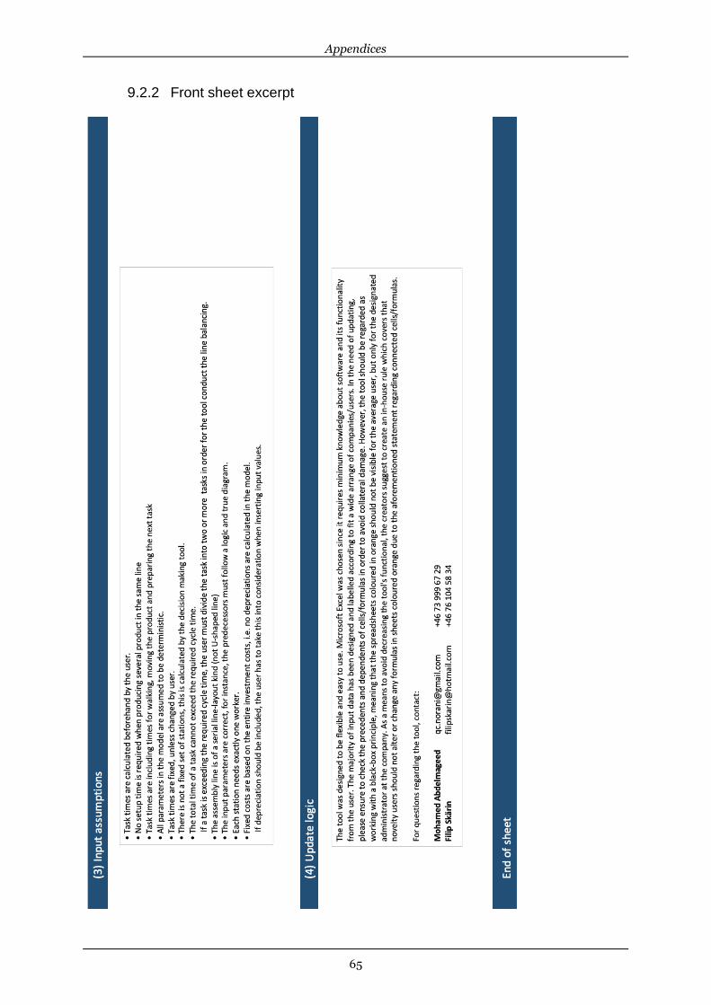
Appendices
65
9.2.2 Front sheet excerpt

Appendices
66
9.2.3 Line balancing input data excerpt
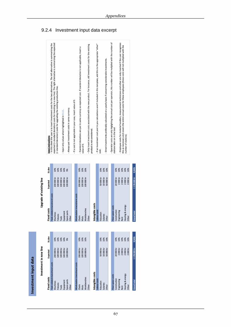
Appendices
67
9.2.4 Investment input data excerpt

Appendices
68
9.2.5 Combining of task times for MMLB excerpt

Appendices
69
9.2.6 MMLB Line ABC WATT excerpt

Appendices
70
9.2.7 MMLB Line ABC MTT excerpt
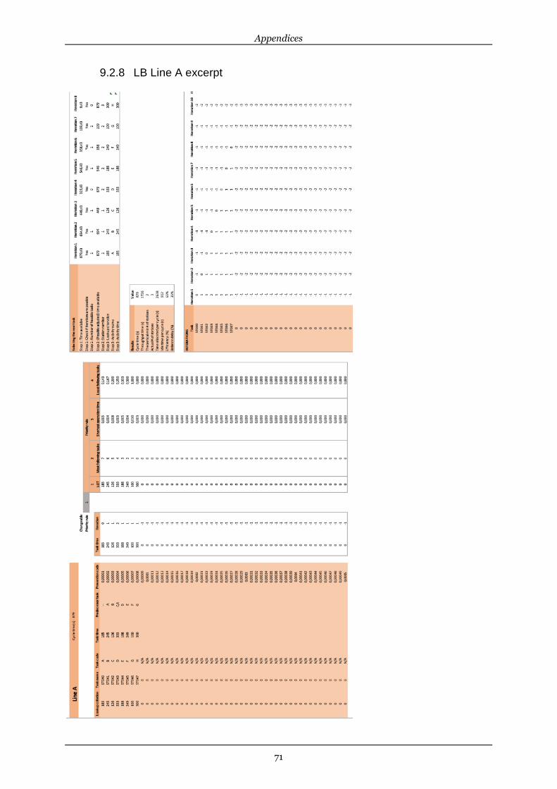
Appendices
71
9.2.8 LB Line A excerpt
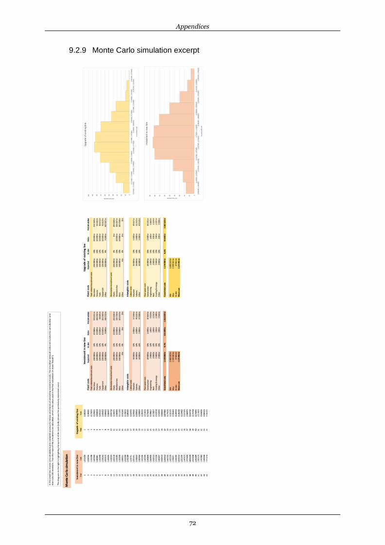
Appendices
72
9.2.9 Monte Carlo simulation excerpt

Appendices
73
9.2.10 Detailed results excerpt

Appendices
74
9.2.11 Station allocation display
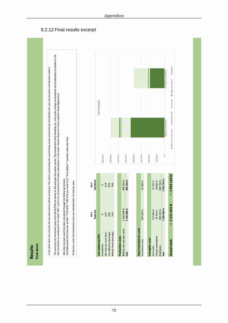
Appendices
75
9.2.12 Final results excerpt