Airshark: Detecting Non-WiFi RF Devicesusing Commodity WiFi Hardware

Shravan Rayanchu, Ashish Patro, Suman Banerjee

{shravan, patro, suman}@cs.wisc.edu

University of Wisconsin, Madison, USA

ABSTRACTIn this paper, we propose Airshark—a system that detectsmultiple non-WiFi RF devices in real-time and using onlycommodity WiFi hardware. To motivate the need forsystems like Airshark, we start with measurement studythat characterizes the usage and prevalence of non-WiFidevices across many locations. We then present the design andimplementation of Airshark. Airshark extracts unique featuresusing the functionality provided by a WiFi card to detectmultiple non-WiFi devices including fixed frequency devices(e.g., ZigBee, analog cordless phone), frequency hoppers(e.g., Bluetooth, game controllers like Xbox), and broadbandinterferers (e.g., microwave ovens). Airshark has an averagedetection accuracy of 91�96%, even in the presence ofmultiple simultaneously active RF devices operating at awide range of signal strengths (�80 to �30 dBm), whilemaintaining a low false positive rate. Through a deploymentin two production WLANs, we show that Airshark can bea useful tool to the WLAN administrators in understandingnon-WiFi interference.

Categories and Subject DescriptorsC.2.1 [Network Architecture and Design]: WirelessCommunication

General TermsDesign, Experimentation, Measurement, Performance

KeywordsWiFi, 802.11, Spectrum, Non-WiFi, RF Device Detection,Interference, Wireless Network Monitoring

1. INTRODUCTIONThe unlicensed wireless spectrum continues to be home

for a large range of devices. Examples include cordlessphones, Bluetooth headsets, various types of audio and videotransmitters (security cameras and baby monitors), wirelessgame controllers (Xbox and Wii), various ZigBee devices (e.g.,

Permission to make digital or hard copies of all or part of this work for

personal or classroom use is granted without fee provided that copies are

not made or distributed for profit or commercial advantage and that copies

bear this notice and the full citation on the first page. To copy otherwise, to

republish, to post on servers or to redistribute to lists, requires prior specific

permission and/or a fee.

IMC’11, November 2–4, 2011, Berlin, Germany.

Copyright 2011 ACM 978-1-4503-1013-0/11/11 ...$10.00.

0

0.2

0.4

0.6

0.8

1

-100 -90 -80 -70 -60 -50 -40 -30

No

rm.

UD

P T

hro

ug

hp

ut

RSSI (dBm)

Analog phone

Videocam

Analog PhoneAudioTx

BluetoothFHSS Phone

VideocamMicrowave

XboxZigbee

Figure 1: Degradation in UDP throughput of a good quality WiFilink (WiFi transmitter and receiver were placed 1m apart) inthe presence of non-WiFi devices operating at different signalstrengths.

-90

-75

-60

-45

-30

-15

14:00 16:00 18:00 20:00 22:00 0:00 2:00 4:00 6:00 8:00 10:00 12:00 14:00

RS

SI

(dB

m)

Time (hour:min)

Microwave OvenBluetooth

Game ControllerFHSS Phone

Analog PhoneZigbee

Figure 2: Average RSSI from different non-WiFi RF deviceinstances shown against the device start times. Measurementswere taken at a dorm-style apartment (location L16, dataset §2)for a 24 hour period.

for lighting and HVAC controls), even microwave ovens, andthe widely deployed WiFi Access Points (APs) and clients.Numerous anecdotal studies have demonstrated that linksusing WiFi, which is a dominant communication technologyin this spectrum, are often affected by interference from all ofthese different transmitters in the environment. In Figure 1,we present results from our own experiments where a single,good quality WiFi link was interfered by different non-WiFidevices—an analog phone, a Bluetooth device, a videocam,an Xbox controller, an audio transmitter, a frequency hoppingcordless phone, a microwave, and a ZigBee transmitter—whenplaced at different distances from the WiFi link.

The figure shows the normalized UDP throughput underinterference, relative to the un-interfered WiFi link, as afunction of the interfering signal strength from these differentdevices. While all of these devices impede WiFi performanceto a certain degree, some of these devices, e.g., the videocamand the analog phone, can totally disrupt WiFi communicationwhen they are close enough (� 80% degradation at RSSI� �70 dBm, and throughput drops to zero in some cases).

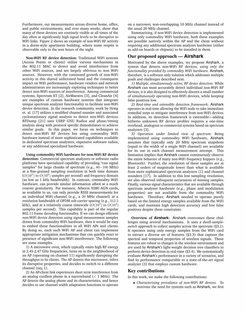
Furthermore, our measurements across diverse home, office,and public environments, and over many weeks, show thatmany of these devices are routinely visible at all times of theday often at significantly high signal levels to be disruptive toWiFi links. Figure 2 shows an example of non-WiFi RF activityin a dorm-style apartment building, where some respite isobservable only in the wee hours of the night.

Non-WiFi RF device detection: Traditional WiFi systems(Access Points or clients) utilize various mechanisms inthe 802.11 MAC to detect and avoid interference fromother WiFi sources, and are largely oblivious to non WiFisources. However, with the continued growth of non-WiFiactivity in this shared unlicensed band and the consequentimpact on WiFi performance, hardware vendors and networkadministrators are increasingly exploring techniques to betterdetect non-WiFi sources of interference. Among commercialsystems, Spectrum XT [2], AirMaestro [3], and CleanAir [4]are examples of custom hardware systems that integrateunique spectrum analyzer functionality to facilitate non-WiFidevice detection. In the research community, work by Honget. al. [17] utilizes a modified channel sounder and associatedcyclostationary signal analysis to detect non-WiFi devices.RFDump [21] uses USRP GNU Radios and phase/timinganalysis along with protocol specific demodulators to achievesimilar goals. In this paper, we focus on techniques todetect non-WiFi RF devices but using commodity WiFihardware instead of more sophisticated capabilities availablein dedicated spectrum analyzers, expensive software radios,or any additional specialized hardware.

Using commodity WiFi hardware for non-WiFi RF devicedetection: Commercial spectrum analyzers or software radioplatforms have specialized capability of providing “raw signalsamples” for large chunks of spectrum (e.g., 80�100 MHz)at a fine-grained sampling resolution in both time domain(O(10

5) to O(10

6) samples per second) and frequency domain

(as low as 1 kHz bandwidth). In contrast, commodity WiFihardware, can provide similar information albeit at a muchcoarser granularity. For instance, Atheros 9280 AGN cards,as available to us, can only provide RSSI measurements foran individual WiFi channel (e.g., a 20 MHz channel) at aresolution bandwidth of OFDM sub-carrier spacing (e.g., 312.5kHz), and at a relatively coarse timescale (O(10

3) to O(10

4)

samples per second). This capability is part of the regular802.11 frame decoding functionality. If we can design efficientnon-WiFi device detection using signal measurement samplesdrawn from commodity WiFi hardware, then it would be easyto embed these functionalities in all WiFi APs and clients.By doing so, each such WiFi AP and client can implementappropriate mitigation mechanisms that can quickly react topresence of significant non-WiFi interference. The followingare some examples.

1) A microwave oven, which typically emits high RF energyin 2.45-2.47 GHz frequencies, turns on in the neighborhood ofan AP (operating on channel 11) significantly disrupting thethroughput to its clients. The AP detects this microwave, infersits disruptive properties, and decides to switch to a differentchannel (say, 1).

2) An AP-client link experiences short term interference froman analog cordless phone in a narrowband (< 1 MHz). TheAP detects the analog phone and its characteristics, and hencedecides to use channel width adaptation functions to operate

on a narrower, non-overlapping 10 MHz channel instead ofthe usual 20 MHz channel.

Summarizing, if non-WiFi device detection is implementedusing only commodity WiFi hardware, both these examplesare possible natively within the AP and the client withoutrequiring any additional spectrum analyzer hardware (eitheras add-on boards or chipsets) to be installed in them.

Our proposed approach — AirsharkMotivated by the above examples, we propose Airshark, asystem that detects non-WiFi RF devices, using only thefunctionality provided by commodity WiFi hardware. Airshark,therefore, is a software-only solution which addresses multiplegoals and challenges described next.

1) Multiple, simultaneously active, RF device detection: WhileAirshark can most accurately detect individual non-WiFi RFdevices, it is also designed to effectively discern a small numberof simultaneously operating non-WiFi devices, while keepingfalse positives low.

2) Real-time and extensible detection framework: Airshark

operates in real-time allowing the WiFi node to take immediateremedial steps to mitigate interference from non-WiFi devices.In addition, its detection framework is extensible—addinghitherto unknown RF device profiles requires a one-timeoverhead, analogous to commercial systems based on spectrumanalyzers [3].

3) Operation under limited view of spectrum: Beingimplemented using commodity WiFi hardware, Airshark

assumes that typically only 20 MHz spectrum snapshots(equal to the width of a single WiFi channel) are availablefor its use in each channel measurement attempt. Thislimitation implies that Airshark cannot continuously observethe entire behavior of many non-WiFi frequency hoppers (e.g.,Bluetooth). Further, the resolution of these samples are atleast 2 orders of magnitude lower than what is availablefrom more sophisticated spectrum analyzers [1] and channelsounders [17]. In addition to this low sampling resolution,we also observed infrequent occurances of missing samples.Finally, various signal characteristics that are available throughspectrum analyzer hardware (e.g., phase and modulationproperties) are not available from the commodity WiFihardware. Therefore, Airshark needed to operate purelybased on the limited energy samples available from the WiFicards, and maintain high detection accuracy and low falsepositives despite these constraints.

Overview of Airshark: Airshark overcomes these chal-lenges using several mechansisms. It uses a dwell-sample-switch approach to collect samples across the spectrum (§3.1).It operates using only energy samples from the WiFi cardto extract a diverse set of features (§3.3) that capture thespectral and temporal properties of wireless signals. Thesefeatures are robust to changes in the wireless environment andare used by Airshark’s light-weight decision tree classifiers toperform device detection in real-time (§3.4). We systematicallyevaluate Airshark’s performance in a variety of scenarios, andfind its performance comparable to a state-of-the-art signalanalyzer [3] that employs custom hardware.

Key contributionsIn this work, we make the following contributions:

• Characterizing prevalance of non-WiFi RF devices. Tomotivate the need for systems such as Airshark, we first

RF Device Category Device Models (set up) Airshark’s Accuracy(low RSSI — high RSSI)

High duty, fixed frequency devices — spectral signature, duty, center frequency, bandwidthAnalog Cordless Phones Uniden EXP4540 Compact Cordless Phone (phone call) 97.73%—100%

Wireless Video Cameras Pyrus Electronics Surveillance Camera (video streaming) 92.7%—99.82%Frequency hoppers — pulse signature, timing signature, pulse spread

Bluetooth devices (ACL/SCO) Bluetooth-enabled devices: (i) iPhone, (ii) iPod touch, (iii) Microsoft notebook mouse 5000,91.63%—99.46%(iv) Jabra bluetooth headset (data transfer/audio streaming)

FHSS Cordless Base/Phones Panasonic 2.4 KX-TG2343 Cordless Base/Phones (phone call) 96.47%—100%

Wireless Audio Transmitter GOGroove PurePlay 2.4 GHz Wireless headphones (audio streaming) 91.23%—99.37%Wireless Game Contollers (i) Microsoft Xbox, (ii) Nintendo Wii, (iii) Sony Playstation 3 (gaming) 91.75%—99%

Broadband interferers — timing signature, sweep detectionMicrowave Ovens (residential) (i) Whirlpool MT4110, (ii) Daewoo KOR-630A, (iii) Sunbeam SBM7500W (heating water/food) 93.16%—99.56%Variable duty, fixed frequency devices — spectral signature, pulse signatureZigBee Devices Jennic JN5121/JN513x based devices (bulk data transfer) 96.23%—99.12%

Table 1: Devices tested with the current implementation of Airshark. Features used to detect the devices include: Pulse signature(duration, bandwidth, center frequency), Spectral signature, Timing signature, Duty cycle, Pulse spread and device specific features(e.g., Sweep detection for Microwave Ovens). Accurac y tests were done in presence of multiple active RF devices and RSSI values rangefrom �80 dBm (low) to �30 dBm (high).

performed a detailed measurement study to characterizethe prevalence of non-WiFi RF devices in typical envi-ronments — homes, offices, and various public spaces.This study was conducted for more than 600 hours overseveral weeks across numerous representative locationsusing signal analyzers [3] that establish the ground truth.

• Design and implementation of Airshark to detect non-WiFiRF devices. Airshark extracts a unique set of featuresusing the functionality provided by a WiFi card, andaccurately detects multiple RF devices (across multiplemodels listed in Table 1) while maintaining a low falsepositive rate (§4). Across multiple RF environments,and in the presence of multiple RF devices operatingsimultaneously, average detection accuracy was 96% atmoderate to high signal strengths (��60 dBm). At lowsignal strengths (�80 dBm), accuracy was 91%. Further,Airshark’s performance is comparable to commercialsignal analyzers (§4.1.6).

• Example uses of Airshark. Through a deployment in twoproduction WLANs, we demonstrate Airshark’s potentialin monitoring the RF activity, and understanding perfor-mance issues that arise due to non-WiFi interference.

To the best of our knowledge, Airshark is the first systemthat provides a generic, scalable framework to detect non-WiFi RF devices using only commodity WiFi cards and enablesnon-WiFi interference detection in today’s WLANs.

2. CHARACTERIZING PREVALENCE OFNON-WIFI RF DEVICES

In this section, we aim to characterize the prevalence andusage of non-WiFi RF devices in real world networks. First, wedescribe our measurement equipment, and data sets.

Hardware. We use AirMaestro RF signal analyzer [3] todetermine the ground truth about the prevalence of RFdevices. This device uses a specialized hardware (BSP2500RF signal analyzer IC), which generates spectral samples(FFTs) at a very high resolution (every 6 µs, with a resolutionbandwidth of 156 kHz) and performs signal processing todetect and classify RF interferers accurately.

— “Ground truth” validation. Before using AirMaestro tounderstand the ground truth about the prevalence of non-

RS

SI (d

Bm

)

Location

-100

-80

-60

-40

-20

0

0 5 10 15 20

Inst

ance

s/hr.

Location

(Cafes) (Enterprises) (Homes)

0

10

20

30

0 5 10 15 20

Figure 3: Distribution of (i) non-WiFi device instances/hourat different locations (top), and (ii) RSSI of non-WiFi devicesat these locations (bottom). Min, Max, 25th, 50th and 75thpercentiles are shown.

WiFi devices, we benchmarked its performance in terms of (i)device detection accuracy and (ii) false positives. We activateddifferent combinations of RF devices (up to 8 devices, listed inTable 1) by placing them at random locations and measuringthe accuracy at different signal strengths (up to �100 dBm).Measurements were done during late nights to avoid anyexternal non-WiFi interference. Our results indicate an overalldetection accuracy of 98.7% with no false positives. The fewcases where AirMaestro failed to detect the devices occurredwhen the devices were operating at very low signal strengths( �90 dBm).Data sets. We collected the RF device usage measurementsusing the signal analyzer at 21 locations for a total of 640hours. We broadly categorize these locations into threecategories: (i) cafes (L1-L7): these included coffee shops,malls, book-stores (ii) enterprises (L8-L14): offices, universitydepartments, libraries and (iii) homes (L15-L21): theseincluded apartments and independent houses. Measurementswere taken over a period of 5 weeks. At some locations, wecould collect data for more than 24 hours (e.g., enterprises,homes) but for others we could collect measurements onlyduring the day times (e.g., coffee shops, malls). We nowsummarize our observations from this data.

Non-WiFi devices are prevalent across locations and often appearwith fairly high signal strengths.

Figure 3 (top) shows the distribution of non-WiFi deviceinstances observed per hour in different wireless environments.

0

25

50

75

100

1 2 3 4 5 6 7 8 9 10 11 12 13 14 15 16 17 18 19 20 21

% I

nst

an

ces

Locations

ZigbeeVideocam

MouseXbox

UnclassifiedJammer

MicrowaveInv. Microwave

FHSS phoneDSS phone

BluetoothAnalog phone

Figure 4: Distribution of non-WiFi device instances at variouslocations.

0

0.2

0.4

0.6

0.8

1

0.1 1 10 100

CD

F

Time (in minutes)

BluetoothFHSS Phone

XboxMouse

0

0.2

0.4

0.6

0.8

1

-90 -80 -70 -60 -50 -40 -30 -20 -10

CD

F

RSSI (dBm)

Analog PhoneMicrowave

VideoCamDSSS Phone

Figure 5: Distribution of (a) Session durations of the non-WiFidevice instances (X-axis in log-scale) and (b) RSSIs of the non-WiFi device instances aggregated across all locations.

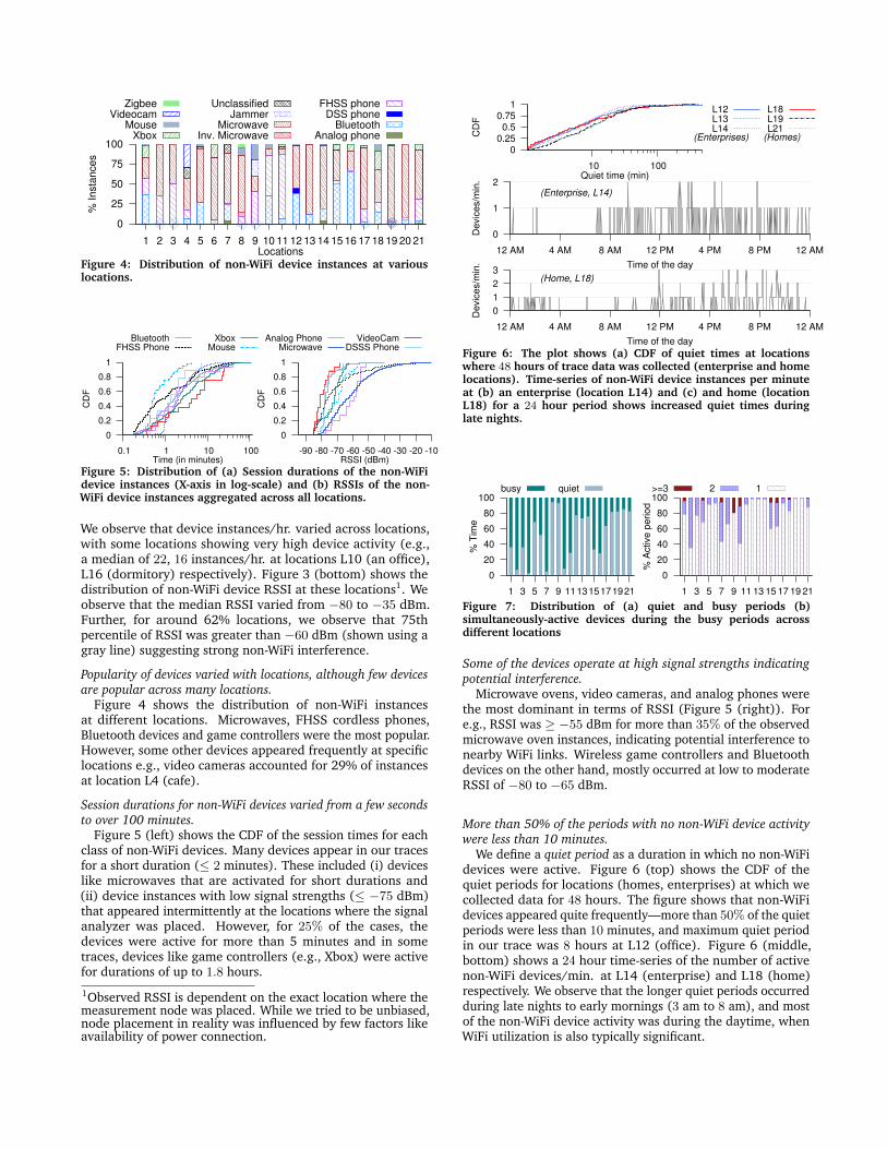
We observe that device instances/hr. varied across locations,with some locations showing very high device activity (e.g.,a median of 22, 16 instances/hr. at locations L10 (an office),L16 (dormitory) respectively). Figure 3 (bottom) shows thedistribution of non-WiFi device RSSI at these locations1. Weobserve that the median RSSI varied from �80 to �35 dBm.Further, for around 62% locations, we observe that 75thpercentile of RSSI was greater than �60 dBm (shown using agray line) suggesting strong non-WiFi interference.

Popularity of devices varied with locations, although few devicesare popular across many locations.

Figure 4 shows the distribution of non-WiFi instancesat different locations. Microwaves, FHSS cordless phones,Bluetooth devices and game controllers were the most popular.However, some other devices appeared frequently at specificlocations e.g., video cameras accounted for 29% of instancesat location L4 (cafe).

Session durations for non-WiFi devices varied from a few secondsto over 100 minutes.

Figure 5 (left) shows the CDF of the session times for eachclass of non-WiFi devices. Many devices appear in our tracesfor a short duration ( 2 minutes). These included (i) deviceslike microwaves that are activated for short durations and(ii) device instances with low signal strengths ( �75 dBm)that appeared intermittently at the locations where the signalanalyzer was placed. However, for 25% of the cases, thedevices were active for more than 5 minutes and in sometraces, devices like game controllers (e.g., Xbox) were activefor durations of up to 1.8 hours.1Observed RSSI is dependent on the exact location where themeasurement node was placed. While we tried to be unbiased,node placement in reality was influenced by few factors likeavailability of power connection.

0

1

2

3

12 AM 4 AM 8 AM 12 PM 4 PM 8 PM 12 AM

Devi

ces/

min

.

Time of the day

(Home, L18)

0

1

2

12 AM 4 AM 8 AM 12 PM 4 PM 8 PM 12 AM

Devi

ces/

min

.

Time of the day

(Enterprise, L14)

0 0.25 0.5

0.75 1

10 100

CD

F

Quiet time (min)

(Enterprises) (Homes)

L12L13L14

L18L19L21

Figure 6: The plot shows (a) CDF of quiet times at locationswhere 48 hours of trace data was collected (enterprise and homelocations). Time-series of non-WiFi device instances per minuteat (b) an enterprise (location L14) and (c) and home (locationL18) for a 24 hour period shows increased quiet times duringlate nights.

0

20

40

60

80

100

1 3 5 7 9 111315171921

% T

ime

busy quiet

0

20

40

60

80

100

1 3 5 7 9 11 13 15 17 19 21

% A

ctiv

e p

eriod

>=3 2 1

Figure 7: Distribution of (a) quiet and busy periods (b)simultaneously-active devices during the busy periods acrossdifferent locations

Some of the devices operate at high signal strengths indicatingpotential interference.

Microwave ovens, video cameras, and analog phones werethe most dominant in terms of RSSI (Figure 5 (right)). Fore.g., RSSI was � �55 dBm for more than 35% of the observedmicrowave oven instances, indicating potential interference tonearby WiFi links. Wireless game controllers and Bluetoothdevices on the other hand, mostly occurred at low to moderateRSSI of �80 to �65 dBm.

More than 50% of the periods with no non-WiFi device activitywere less than 10 minutes.

We define a quiet period as a duration in which no non-WiFidevices were active. Figure 6 (top) shows the CDF of thequiet periods for locations (homes, enterprises) at which wecollected data for 48 hours. The figure shows that non-WiFidevices appeared quite frequently—more than 50% of the quietperiods were less than 10 minutes, and maximum quiet periodin our trace was 8 hours at L12 (office). Figure 6 (middle,bottom) shows a 24 hour time-series of the number of activenon-WiFi devices/min. at L14 (enterprise) and L18 (home)respectively. We observe that the longer quiet periods occurredduring late nights to early mornings (3 am to 8 am), and mostof the non-WiFi device activity was during the daytime, whenWiFi utilization is also typically significant.

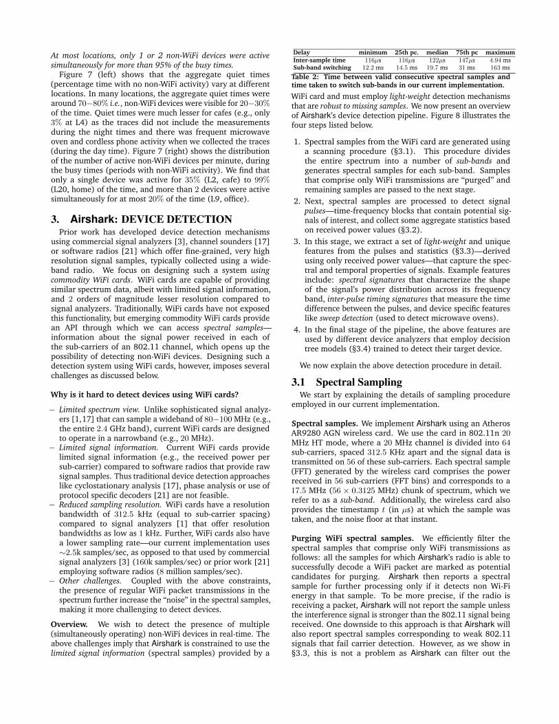
At most locations, only 1 or 2 non-WiFi devices were activesimultaneously for more than 95% of the busy times.

Figure 7 (left) shows that the aggregate quiet times(percentage time with no non-WiFi activity) vary at differentlocations. In many locations, the aggregate quiet times werearound 70�80% i.e., non-WiFi devices were visible for 20�30%

of the time. Quiet times were much lesser for cafes (e.g., only3% at L4) as the traces did not include the measurementsduring the night times and there was frequent microwaveoven and cordless phone activity when we collected the traces(during the day time). Figure 7 (right) shows the distributionof the number of active non-WiFi devices per minute, duringthe busy times (periods with non-WiFi activity). We find thatonly a single device was active for 35% (L2, cafe) to 99%

(L20, home) of the time, and more than 2 devices were activesimultaneously for at most 20% of the time (L9, office).

3. Airshark: DEVICE DETECTIONPrior work has developed device detection mechanisms

using commercial signal analyzers [3], channel sounders [17]or software radios [21] which offer fine-grained, very highresolution signal samples, typically collected using a wide-band radio. We focus on designing such a system usingcommodity WiFi cards. WiFi cards are capable of providingsimilar spectrum data, albeit with limited signal information,and 2 orders of magnitude lesser resolution compared tosignal analyzers. Traditionally, WiFi cards have not exposedthis functionality, but emerging commodity WiFi cards providean API through which we can access spectral samples—information about the signal power received in each ofthe sub-carriers of an 802.11 channel, which opens up thepossibility of detecting non-WiFi devices. Designing such adetection system using WiFi cards, however, imposes severalchallenges as discussed below.

Why is it hard to detect devices using WiFi cards?

� Limited spectrum view. Unlike sophisticated signal analyz-ers [1,17] that can sample a wideband of 80�100 MHz (e.g.,the entire 2.4 GHz band), current WiFi cards are designedto operate in a narrowband (e.g., 20 MHz).

� Limited signal information. Current WiFi cards providelimited signal information (e.g., the received power persub-carrier) compared to software radios that provide rawsignal samples. Thus traditional device detection approacheslike cyclostationary analysis [17], phase analysis or use ofprotocol specific decoders [21] are not feasible.

� Reduced sampling resolution. WiFi cards have a resolutionbandwidth of 312.5 kHz (equal to sub-carrier spacing)compared to signal analyzers [1] that offer resolutionbandwidths as low as 1 kHz. Further, WiFi cards also havea lower sampling rate—our current implementation uses⇠2.5k samples/sec, as opposed to that used by commercialsignal analyzers [3] (160k samples/sec) or prior work [21]employing software radios (8 million samples/sec).

� Other challenges. Coupled with the above constraints,the presence of regular WiFi packet transmissions in thespectrum further increase the “noise” in the spectral samples,making it more challenging to detect devices.

Overview. We wish to detect the presence of multiple(simultaneously operating) non-WiFi devices in real-time. Theabove challenges imply that Airshark is constrained to use thelimited signal information (spectral samples) provided by a

Delay minimum 25th pc. median 75th pc maximumInter-sample time 116µs 116µs 122µs 147µs 4.94 msSub-band switching 12.2 ms 14.5 ms 19.7 ms 31 ms 163 msTable 2: Time between valid consecutive spectral samples andtime taken to switch sub-bands in our current implementation.

WiFi card and must employ light-weight detection mechanismsthat are robust to missing samples. We now present an overviewof Airshark’s device detection pipeline. Figure 8 illustrates thefour steps listed below.

1. Spectral samples from the WiFi card are generated usinga scanning procedure (§3.1). This procedure dividesthe entire spectrum into a number of sub-bands andgenerates spectral samples for each sub-band. Samplesthat comprise only WiFi transmissions are “purged” andremaining samples are passed to the next stage.

2. Next, spectral samples are processed to detect signalpulses—time-frequency blocks that contain potential sig-nals of interest, and collect some aggregate statistics basedon received power values (§3.2).

3. In this stage, we extract a set of light-weight and uniquefeatures from the pulses and statistics (§3.3)—derivedusing only received power values—that capture the spec-tral and temporal properties of signals. Example featuresinclude: spectral signatures that characterize the shapeof the signal’s power distribution across its frequencyband, inter-pulse timing signatures that measure the timedifference between the pulses, and device specific featureslike sweep detection (used to detect microwave ovens).

4. In the final stage of the pipeline, the above features areused by different device analyzers that employ decisiontree models (§3.4) trained to detect their target device.

We now explain the above detection procedure in detail.

3.1 Spectral SamplingWe start by explaining the details of sampling procedure

employed in our current implementation.

Spectral samples. We implement Airshark using an AtherosAR9280 AGN wireless card. We use the card in 802.11n 20

MHz HT mode, where a 20 MHz channel is divided into 64

sub-carriers, spaced 312.5 KHz apart and the signal data istransmitted on 56 of these sub-carriers. Each spectral sample(FFT) generated by the wireless card comprises the powerreceived in 56 sub-carriers (FFT bins) and corresponds to a17.5 MHz (56 ⇥ 0.3125 MHz) chunk of spectrum, which werefer to as a sub-band. Additionally, the wireless card alsoprovides the timestamp t (in µs) at which the sample wastaken, and the noise floor at that instant.

Purging WiFi spectral samples. We efficiently filter thespectral samples that comprise only WiFi transmissions asfollows: all the samples for which Airshark’s radio is able tosuccessfully decode a WiFi packet are marked as potentialcandidates for purging. Airshark then reports a spectralsample for further processing only if it detects non Wi-Fienergy in that sample. To be more precise, if the radio isreceiving a packet, Airshark will not report the sample unlessthe interference signal is stronger than the 802.11 signal beingreceived. One downside to this approach is that Airshark willalso report spectral samples corresponding to weak 802.11signals that fail carrier detection. However, as we show in§3.3, this is not a problem as Airshark can filter out the

Spectral

samples

Pulse

Detector

new pulses Pulse Matching

Stats

extend

add new pulse

terminate

(avg. duty, avg. power, ..)

Completed

pulses

Duty

Analog Phone Analyzer

active

pulses

Spectral

signature

Sweep

analyzer

Timing

signature

FHSS Phone Analyzer

Sub-band

change

WiFi Card

(Frequency hopping device analyzers)

Microwave Analyzer

Pulse

signature

Decision tree-based device detection

CF

BW

Dura

tion

Pulse

spread

(Fixed frequency device analyzers)

Generic Feature Extraction

Tagged pulses,

statistics

Decision

Tree

Bluetooth Analyzer

3

42 Pulse detection, Stats collection

1 Spectral

sampling

(Section 3.1)

(Section 3.2)

(Section 3.3)

(Section 3.4)

Figure 8: (a) Illustration of Airshark’s detection pipeline. Spectral samples from the WiFi card are generated using a scanning procedure(§3.1). These samples are processed to detect signal pulses, and collect some aggregate statistics based on the received power values(§3.2). In the next stage, various features capturing the spectral and temporal properties of the signals are extracted (§3.3), and areused by different device analyzers that employ decision tree models (§3.4) trained to detect their target RF devices.

samples relevant to non-WiFi transmissions by employingdevice detection mechanisms. We term the samples reportedby Airshark after this purging step as valid spectral samples.

Scanning procedure. Airshark divides the entire spectrum(e.g., 80 MHz) into several (possibly overlapping) sub-bands,and samples one sub-band at a time. Our current implementa-tion uses 7 sub-bands with center frequencies correspondingto the WiFi channels 1, 3, 6, 9, 11, 13 and 14. Table 2 shows(i) inter-sample time: the time between two consecutive validspectral samples (within a sub-band) and (ii) time takento switch the sub-bands. Increased gap in the inter-sampletime for a few samples (� 150µs) is due to the nature ofthe wireless environment—in the absence of strong non-WiFidevices transmissions, intermittent interference from WiFitransmissions causes gaps due to purged spectral samples.Sampling gaps are also caused when switching sub-bands(⇠ 20 ms on an average, and 163 ms in the worst case).

To amoritize the cost of switching sub-bands, Air-

shark employs a dwell-sample-switch approach to sampling:Airshark dwells for 100 ms in each sub-band, captures thespectral samples and then switches to the next sub-band.As we show later, in spite of the increased gap for fewsamples, we find the sampling resolution of current WiFicards to be adequate in detecting devices (across differentwireless environments) with a reasonable accuracy (§4). In§4, we demonstrate the adversarial case where strong WiFiinterference coupled with weak non-WiFi signal transmissionscan affect Airshark’s detection capabilities.

3.2 Extracting signal dataWe now explain the next stage in the detection pipeline

that operates on the spectral samples to generate signal pulses,along with some aggregate statistics.

“Pulse” Detection. Each spectral sample is processed toidentify the signal “peaks”. Several complex mechanismshave been proposed for peak detection [11,16]. To keep ourimplementation efficient, we use a simple and a fairly standardalgorithm [12,14]—peaks are identified by searching for “localmaximas” that are above a minimum energy threshold �

s

.For each peak, the pulse detector generates a pulse as a set

�s

kp3

p1 p2

Pow

er

kp4

spectral sample

p4

add

peaks

t2

Frequency

t0

t1

new

pulses

Frequency

Tim

e

p3

active pulses

match

terminate

t2

extend

Figure 9: Illustration of the pulse detection and matchingprocedure. Pulse detector processes the spectral sample at timet2 to output two new pulses p3 and p4. New pulse p3 matcheswith the active pulse p1, and results in extending p1. Active pulsep2 is terminated as there is no matching new pulse, and newpulse p4 is added to the active pulse list.

of contiguous FFT bins that surround this peak. A pulsecorresponds to a signal of interest, and its start and endfrequencies are computed as explained below.

— frequency and bandwidth estimation: Let kp

denote thepeak bin and p(k

p

) denote the power received in this bin.We first find the set of contiguous FFT bins [k0

s

, k0e

] suchthat k0

s

kp

k0e

and power received in each bin is (i)above the energy threshold, �

s

and (ii) within �B

of the peakpower p(k

p

) i.e., p(k) � �s

Vp(k

p

)� p(k) < �B

8k 2 [k0s

, k0e

].The center frequency (CF) and the bandwidth (BW) of apulse corresponding to this peak bin can be characterizedby considering its mean localization and dispersion in thefrequency domain:

kc

=

1X

k

p(k)

X

k

k·p(k), k0s

k k0e

B = 2

vuuut1X

k

p(k)

X

k

(k � kc

)

2·p(k), k0s

k k0e

The center frequency bin kc

is computed as the center point ofthe power distribution, and the frequency spread around thiscenter point is defined as the bandwidth B of the pulse. Foreach peak, we restrict the bandwidth of interest to comprisebins whose power values are more than �

s

and are within�B

of the peak power p(kp

). We use this mechanism as it issimple to compute and it provides reasonable estimates as weshow in §4. Based on the computed bandwidth, the start bin(k

s

) and the end bin (ke

) are determined. The pulse detector

-105

-90

-75

-60

-45

-30

0 10 20 30 40 50 60

Sig

na

l str

en

gth

(d

Bm

)

Frequency bins (0-55)

1m2m3m5m

10m15m20m

-0.16

-0.14

-0.12

-0.1

-0.08

-0.06

-0.04

0 10 20 30 40 50 60N

orm

aliz

ed

Po

we

rFrequency bins (0-55)

1m2m3m5m

10m15m20m

Figure 10: (a) Distribution of average power vs. frequency foran analog cordless phone at different distances. (b) Spectralsignatures for the analog cordless phone are not affected for RSSIvalues of � �80 dBm.

can potentially output multiple pulses for a spectral sample.Each pulse in a spectral sample observed at time t can berepresented using the tuple [t, k

s

, kc

, ke

, [p(ks

) . . . p(ke

)]]

Pulse Matching. Airshark maintains a list of active pulses forthe current sub-band. This active pulse list is empty at thestart of the sub-band, and the first set of pulses (obtained afterprocessing a spectral sample in the sub-band) are added to thislist as active pulses. For the rest of the samples in the sub-band,a pulse matching procedure is employed: the pulse detectoroutputs a set of new pulses after processing the sample. Thesenew pulses are compared against the list of active pulses todetermine a match. In our current implementation, we use astrict criteria to determine a match between a new pulse andan active pulse: the CFs and BWs of the new pulse and theactive pulse must be equal, and their peak power values mustbe within 3 dB (to accommodate signal strength variations).Once a match is determined, the new pulse is merged with theactive pulse to extend it i.e., the duration of the active pulseis increased to accommodate this new pulse, and the powervalues of the active pulse are updated by taking a weightedaverage of power values of the new and the active pulse.

After the pulse matching procedure, any left over newpulses in the current spectral sample are added to the activepulse list. The active pulses that did not find a matching newpulse in the current sample are terminated. Active pulsesare also terminated if Airshark encounters more than onemissing spectral sample (i.e., inter-sample time � 150 µs).Once an active pulse is terminated, it is moved to the currentsub-band’s list of completed pulses. It is possible that someof the active pulses are prematurely terminated due to thestrict match and termination criteria. However, doing so helpsAirshark maintain a low false positive rate as it only operateson well-formed pulses that satisfy this strict criteria (§4).Figure 9 illustrates this pulse detection procedure.

Stats Module. The stats module operates independently ofthe above pulse logic. It processes all the spectral samples of asub-band to generate the following statistics: (i) average power:this is the average power in each FFT bin for the duration ofthe sub-band, (ii) average duty: this is the average duty cyclefor each bin in the sub-band. The duty cycle of an FFT bin kis computed as 1 if p(k)��

s

, otherwise it is 0. (iii) high dutyzones: After processing a sub-band, a mechanism similar topeak detection, followed by CF and BW estimation procedureis applied on the “average power” statistic to identify the high

duty zones in the sub-band. These are used to quickly detectthe presence of high duty devices.

Before switching to the next sub-band, all the active pulsesfor the current sub-band are terminated and pushed to thelist of the sub-band’s completed pulses. The list of completedpulses along with the aggregate statistics are then passed onto the next stage of the pipeline to perform feature extraction.

3.3 Feature ExtractionUsing the completed pulses list and statistics, we extract a

set of generic features that capture the spectral and temporalproperties of different non-WiFi device transmissions. Thesefeatures—frequency, bandwidth, spectral signature, dutycycle, pulse signature, inter-pulse timing signature, pulsespread and device specific features like sweep detection—formthe building blocks of Airshark’s decision tree-based devicedetection mechanisms. We now explain these features.

(F1) Frequency and Bandwidth. Most RF devices operateusing pre-defined center frequencies, and their waveformsoccupy a specific bandwidth. For e.g, a ZigBee device operateson one of the pre-defined 16 channels [22], and occupies abandwidth of 2 MHz. The center frequency and bandwidthof the pulses (and sub-band’s high duty zones) are used asfeatures in Airshark’s decision tree models.

(F2) Spectral signatures. Many RF devices also exhibitcertain power versus frequency characteristics. We capturethis using a spectral signature: given a set of frequency bins[k

s

. . .ke

] and corresponding power values [p(ks

). . .p(ke

)], ifwe treat the frequency bins as a set of orthogonal axes, we canconstruct a vector �!s = p(k

s

)

ˆks

+ . . .+p(ke

)

ˆke

that representsthe power received in each of the bins. We then normalizethis vector to derive a unit vector representing the spectralsignature: ˆs =

�!s

|s| . Given a reference spectral signature ˆsr

anda measured spectral signature ˆs

m

, we compute the similaritybetween the spectral signatures as the angular difference (✓):cos

�1(

ˆsr

· ˆsm

). The angular difference captures the degree ofalignment between the vectors, and is close to 0

� when therelative composition of the vectors is similar.

Spectral signatures can be computed on the average powervalues of the pulses (e.g., ZigBee pulse) or on the high dutyzones (e.g., for high duty devices like analog phones) to aidin device detection. Figure 10 shows the power distributionof an analog cordless phone at different distances, and thecorresponding spectral signatures computed at each distance.The figure shows that normalization aids in making thesignatures robust to the changes in the signal strengths of theRF devices. However, at very low signal strengths ( �90

dBm), the spectral signatures tend to deviate and result in anincreased theta, leading to false negatives (§4).

(F3) Duty cycle. The duty cycle D of a device is the fractionof time the device spends in “active” state. This can beused to identify high duty devices, e.g., analog phones andwireless video cameras have D=1, or identify devices withcharacteristic duty cycles e.g., microwave ovens have D=0.5.In reality, due to the presence of multiple devices, it is possiblefor the duty cycle of the bandwidth (FFT bins) used by a deviceto be more than its expected duty cycle. We therefore use thenotion of minimum duty cycle D

min

for devices (Dmin

=0.5for a microwave oven) as one of the features.

Protocol/Device Bandwidth Duration Frequency usage

WDCT Cordless Phone 0.892 KHz 700 µs FHSS, 90 channelsBluetooth 1 MHz 366 µs - 3 ms FHSS, 79 channelsZigBee 2 MHz < 5 ms Static, 16 channelsGame controller 500 KHz 235 µs FHSS, 40 channels

Table 3: Pulse signatures for different RF devices.

0

20

40

60

80

100

5ms 16.66ms

CD

F

Time

825us625us 10ms

Bluetooth SCOFHSS cordless phone

FHSS cordless base

XboxMicrowave

Figure 11: Inter-pulse timing signature for different devices.

0

0.0025

0.005

0.0075

0.01

0.0125

0 50 100 150 200 250 300 350 400

PD

F

Bin number

AudioTxFHSS Phone

Figure 12: Pulse distribution of FHSS cordless phone and anaudio transmitter as captured by Airshark.

(F4) Pulse signatures. Along with CF and BW, thetransmission durations of many devices conform to theirprotocol standards. For e.g., in Bluetooth, the duration of atransmission slot is 625 µs, out of which 366 µs is spent inactive transmission. Similarly, WDCT cordless phones (FHSSphones) have a pulse duration of 700 µs. Table 3 showsthese properties (frequency, bandwidth, and duration of thepulses) for different devices. Airshark combines these threeproperties together to define pulse signatures for devices thatcommunicate using pulses (e.g., ZigBee, Bluetooth) and usesthem as features in the detection process.

(F5) Inter-pulse timing signatures. Timing between thetransmissions of many devices also exhibit certain properties.In Bluetooth SCO, for example, examining the spectrumwill reveal sets of two consecutive pulses that satisfy theBluetooth pulse signature (Table 3) and are separated by atime difference of 625 µs. WDCT cordless phones and gamecontrollers (e.g., Wii) exhibit similar properties with timedifference between consecutive pulses (occuring at the samecenter frequency) in a set being 5 ms and 825 µs respectively.Similarly, microwaves exhibit an ON-OFF cycle with a periodof 16.6 ms. Figure 11 illustrates these timing properties.

Since Airshark can only sample a particular sub-band ata time, it cannot capture all the pulses of a device. This isespecially true for frequency hopping devices. Due to thenature of sampling, we cannot expect every captured pulse toexhibit the above timing property. Airshark’s device analyzerstherefore use a relaxed constraint—number of pulse setsthat satisfy a particular timing property is used as one of thefeatures in the decision tree models (§3.4).

(F6) Pulse spread. Airshark accumulates the pulses fora number of sub-bands, and extracts features from pulsesbelonging to a particular pulse signature to detect the presenceof frequency hopping devices. Together, these featuresrepresent the pulse spread across different sub-bands.

1. Pulses-per-band (mean and variance). We use the averagenumber of pulses per sub-band, and the correspondingvariance as one of the measures to characterize the pulsespread. For frequency hoppers, we can expect the averagenumber of pulses in each sub-band to be higher (and thevariance lower) compared to fixed frequency devices.

2. Pulse distribution. Pulses of many frequency hoppingdevices tend to conform to a particular distribution. Forexample, FHSS cordless phone pulses are spread uniformlyacross the entire 80 MHz band, whereas, the pulse distributionfor other frequency hoppers like audio transmitters may tendto be concentrated on certain frequencies of sub-bands, asshown in Figure 12. The X-axis shows the bin number b foreach of the seven sub-bands (b

max

= 56 ⇥ 7 = 392), andY-axis shows the fraction of the pulses that fall into each bin.2

Airshark checks whether the distribution of pulses acrossthe sub-bands conforms to an expected pulse distributionusing Normalized Kullback-Leibler Divergence (NKLD) [20],a well known metric in information theory. NKLD is simpleto compute and can be used to quantify the ‘distance’ or therelative entropy between two probability distributions. NKLDis zero when the two distributions are identical, and a highervalue of NKLD implies increased distance between the twodistributions. The definition of NKLD is assymetric, thereforewe use a symmetric version of NKLD [20] to compare twodistributions. Let r(b) be the reference pulse distributionover all the bins (b 2 B = [0, b

max

]), computed over a largeperiod of time. Let m(b) be the measured pulse distributionover a smaller time period t

m

. The symmetric NKLD for twodistributions r(b) and m(b) can be defined as:

NKLD(m(b), r(b)) =1

2

⇣D(m(b)kr(b))H(m(b))

+

D(r(b)km(b))H(r(b))

⌘

where, D(m(b)kr(b)) quantifies the divergence and is com-puted as

Pb2B m(b)

���log m(b)r(b)

���, and H(m(b)) is the entropy ofthe random variable b with distribution m(b) i.e., H(m(b)) =�P

b2B m(b) log2 m(b).While Airshark can measure the pulse distribution m(b)

over a large time scale, and check if it conforms to r(b), thiswill increase the time to detect the device. This leads to thequestion, “what is the minimum time scale t

m

at which thepulse distribution can be measured?" We chose this time scaleby empirically measuring how the NKLD values convergewith the increase in the number of samples under differentconditions. For the devices that we tested, we observed around15000 samples (around 6 scans of the entire 80 MHz band,amounting to 6�7 seconds) was sufficient. We show how thenumber of samples affect the NKLD values in §4.2.3. We notethat not all devices conform to a particular pulse distributione.g., in our experiments, we found variable pulse distributionsfor Bluetooth as it employs adaptive hopping mechanisms.

(F7) Device specific features. Detection accuracy can beimproved by using features unique to the target device. Weillustrate this using a feature specific to microwave ovens.— Sweep detector. The heating source in a residential

2Instead of measuring the actual pulse distribution over the80 MHz band, we stitch the sub-bands together (ignoringthe overlaps) and measuring the pulse distribution over thestitched sub-bands.

Frequency sweep

0 10 20 30 40 50

Frequency bins (CF: bin 28, 2452 MHz)

0

8

16

24

32

40T

ime

(m

s)

-140

-120

-100

-80

-60

-40

-20

sig

na

l str

en

gth

(d

Bm

)

Figure 13: Spectral samples from Airshark capturing the activityof a residential microwave. The plot shows (i) the ON-OFF cyclefor is around 16.6 ms and (ii) “frequency sweeps” during the ONperiods.

microwave oven is based on a single magnetron tube thatgenerates high power electromagnetic waves whenever theinput voltage is above some threshold. This results in anON-OFF pattern, typically periodic with a frequency of 60

Hz (frequency of the AC supply line). Although there mightbe differences between the emissions from ovens of differentmanufacturers, the peak operational power is mostly around2.45-2.47 GHz and during the ON periods, the radiated signalexhibits a frequency sweep of around 4�6 MHz [19,27].

Figure 13 shows the resulting 16.66 ms periodic ON-OFFpattern and the frequency sweeps during the ON periods ofa microwave oven as captured by Airshark. In the currentprototype of Airshark, the microwave oven analyzer includessweep detection, along with timing signature analysis. Wetested 6 microwaves (from different manufacturers), andAirshark was able to detect all of them using these features.

3.4 Device DetectionAirshark uses decision tree [24] based classifiers in order

to detect the presence of RF devices. A decision tree isa mapping from observations about an item (feature set)to conclusions about its target value (class). It employs asupervised learning model where a small set of labeled data,referred to as training data, is first used to build the tree andis later used to classify unlabeled data. In Airshark, we use thepopular C4.5 algorithm [24] to construct the decision trees.For further details about mechanisms to build decision treesand the classification process, we refer the readers to [24].

Airshark employs a separate analyzer for each class ofdevices. These device analyzers operate on a subset offeatures described previously, and make use of decision treeclassifiers trained to detect their corresponding RF devices.The advantages of using per-device classifiers are three-fold:(i) each classifier can use a separate feature subset, (ii)classifiers can operate at different time granularities e.g., fixedfrequency device analyzers (e.g., analog phone) can carryout the classification when Airshark finishes processing asub-band, whereas for frequency hopping device analyzerslike (e.g., Bluetooth, game controllers) the classificationdecision can only take place after enough samples havebeen processed (§3.3), (iii) classification process is moreefficient when multiple devices are simultaneously active—each classifier outputs either label 1 (indicating the presenceof the device), or label 0 (indicating the absence of thedevice). The alternative approach of using a single classifier iscumbersome as it requires training the classifier for all possibledevice combinations (each with a separate label).

Training. Before Airshark can identify a new RF device,its features have to be recorded for training. To do this,

features relevant to this device are identified, and thenextracted from spectral samples for the cases when thedevice is active in isolation (label 1), and when the deviceis inactive (label 0). For example, when adding the analogphone analyzer, we collected the spectral samples when thephone was activated in isolation and when the phone wasinactive. We then instantiated analog phone’s device analyzerto extract these features: bandwidth, spectral signature andduty cycle (measured from the recorded spectral samples)and the list of possible CFs the phone can operate on. It isworth pointing out that identifying the relevant feature set fora device and training the corresponding device analyzer is aone time overhead before adding a new RF device to Airshark.Table 1 lists the feature set employed by device analyzers inour current implementation.

Classification. We now summarize Airshark’s detectionpipeline. Each sample is processed by the first stage of thepipeline, and results in updating the completed pulse listand aggregate statistics. Device analyzers are invoked whenAirshark finishes processing a sub-band:

1. Each device analyzer operates on the completed pulses andaggregate statistics, to derive its features. The featuresmay include: CF, BW, angular difference (correspondingto its spectral signature), duty cycle, number and thespread of the pulses satisfying its pulse signature and timingsignature.

2. The device analyzer’s decision tree is invoked to outputeither label 1 or 0.

3. In case the decision tree outputs label 1, Airshark invokes amodule that tags the selected pulses (satisfying the pulsesignature and timing signature) as “owned" by this RFdevice.

An additional check is performed for frequency hoppingdevice analyzers: if there are not enough accumulated samplesto perform the classification, the classification decision isdeferred to the next sub-band.

Dealing with multiple RF devices and overlapping signals.When multiple RF devices are simultaneously active, thespectrum may be occupied by a large number of transmissions(signal pulses). If the transmissions from multiple devicesdo not overlap in time or in frequency (either because ofthe diversity in the device transmission times, or becausethe devices operate in a non-overlapping spectrum bands),Airshark’s device analyzers can proceed as is. Further, forcertain combinations of devices, transmissions may overlap inboth time and frequency, but not always. For example, this isthe case when frequency hopping devices and fixed-frequency,low duty devices are present. In our benchmarks for thesecombinations, Airshark could always find enough pulses thatdo not overlap, and therefore was able to correctly detect thedevices.

Transmissions from multiple devices that always overlapin time and frequency, however, can decrease the detectionaccuracy if the above techniques are used as is. For example,if the transmissions from a fixed-frequency, always-on device(e.g., analog phone) overlap in frequency with another fixed-frequency device (e.g., ZigBee device), features like spectralsignatures will not perform well. This is because overlappingsignals change the “shape” of the power distribution andincrease the angular difference as shown in Figure 14(a). One

-100

-90

-80

-70

-60

-50

0 27 55

Sig

na

l str

en

gth

(d

Bm

)

FFT bins (0-55)

partial analog phonepartial zigbee

0 0.02 0.04 0.06 0.08 0.1

0.12 0.14

Zigbee Analog

An

gu

lar

diff

. (r

ad

ian

s) complete-matchpartial-match

Figure 14: Overlapping signal detection. (a) partial overlapbetween ZigBee and analog signals (b) using partial matchesbetween spectral signatures reduces the angular difference inoverlapping cases.

approach to resolve such overlaps, is to use cyclostationaryanalysis [17] on raw signal samples. Such rich signalinformation (very high resolution, raw signal samples),however, is not available through WiFi cards. We extendthe basic approach used in Airshark to handle these cases asfollows: device analyzers first identify the potential peaks thatmatch their CFs. For each peak, instead of a complete matchon the signal’s bandwidth BW, a partial match of the spectralsignatures is performed. The bandwidth BW

par

for the partialmatch is decided by the bandwidth detection algorithm, and isrequired to be above a minimum bandwidth BW

min

in order tocontrol the false positives (i.e., BW

min

BWpar

BW). In ourbenchmarks, setting BW

min

to 0.6⇥BW improved the accuracywithout increasing the false positives (§4). Figure 14(b) showsthe reduction in angular difference when using a partial match.

Alternative classifiers. We also built another classifier basedon support vector machines (SVM) [5]. In our experiments, wefound that in most cases, Airshark’s SVM-based and decisiontree based classifiers had similar detection accuracies. In somescenarios involving multiple devices, SVM-based classifierperformed slightly better (§4.1.5). However, we elected touse a decision tree based classifier, as it has very low memoryand processing requirements, thus making it feasible to embednon-WiFi device detection functionality in commodity wirelessAPs and clients.

4. EXPERIMENTAL RESULTSIn this section, we evaluate Airshark’s performance under

a variety of scenarios, and present real-world applicationsof Airshark through a small scale deployment. We start bypresenting the details of our implementation and testbed setup, followed by the metrics used for evaluation.

Implementation. Our implementation of Airshark consists offew hundred lines of C code that sets up the FFT samplingfrom the Atheros AR9280 AGN based wireless card, and about4500 lines of Python scripts that implement the detectionpipeline. We used an off-the-shelf implementation of the C4.5decision tree algorithm [6] for training and classification.For the alternative SVM-based classifier, we used an SVMimplementation [5] employing a radial basis function kernelwith default parameter setting. We focus on detecting devicesin 2.4 GHz spectrum, and our current prototype has beentested with 8 classes of devices (across multiple device models)mentioned in Table 1.

Evaluation set up. We performed all our experiments in auniversity building (except those in §4.1.4). Our trainingdata was taken during the late evenings and night times tominimize the impact of external non-WiFi interference. Our

0

20

40

60

80

100

-100 -90 -80 -70 -60 -50 -40 -30

% A

ccu

racy

RSSI (dBm)

Analog PhoneAudioTx

BluetoothFHSS Phone

Video CameraMicrowave

XboxZigbee

Figure 15: Accuracy of single device detection across signalstrengths for different RF devices.

0 20 40 60 80

100

-100 -90 -80 -70 -60 -50 -40 -30

% A

ccu

racy

RSSI (dBm)

2 devices3 devices

>= 4 devices

Figure 16: Accuracy of detection across signal strengths for 2, 3,and � 4 device combinations.

evaluation experiments, however, were performed over aperiod of one week that included both busy hours and nighttimes. We also used the AirMaestro signal analyzer [3] inorder to determine the “ground truth” about the presence ofany external non-WiFi RF devices during our experiments.

Evaluation Metrics. We use the following metrics to evaluatethe performance of Airshark:1. Detection accuracy: This is the fraction of correctly identifiedRF device instances. This estimates the probability thatAirshark accurately detects the presence of an RF device.2. False positive rate (FPR): This is defined as the fractionof false positives. This estimates the probability thatAirshark incorrectly determines the presence of an RF device.

We will first evaluate Airshark’s performance in variousscenarios, and then comment on the parameters we chose.We set the energy threshold �

s

to �95 dBm, �B

to 10 dB, andfor computing NKLD we use 15000 samples. The RF devicestested and the features used are listed in Table 1.

4.1 Performance evaluationWe start by evaluating Airshark using controlled experi-

ments with different RF devices.

4.1.1 Single device detection accuracy

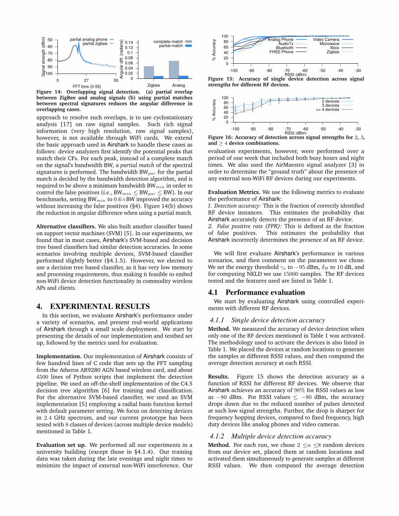
Method. We measured the accuracy of device detection whenonly one of the RF devices mentioned in Table 1 was activated.The methodology used to activate the devices is also listed inTable 1. We placed the devices at random locations to generatethe samples at different RSSI values, and then computed theaverage detection accuracy at each RSSI.

Results. Figure 15 shows the detection accuracy as afunction of RSSI for different RF devices. We observe thatAirshark achieves an accuracy of 98% for RSSI values as lowas �80 dBm. For RSSI values �80 dBm, the accuracydrops down due to the reduced number of pulses detectedat such low signal strengths. Further, the drop is sharper forfrequency hopping devices, compared to fixed frequency, highduty devices like analog phones and video cameras.

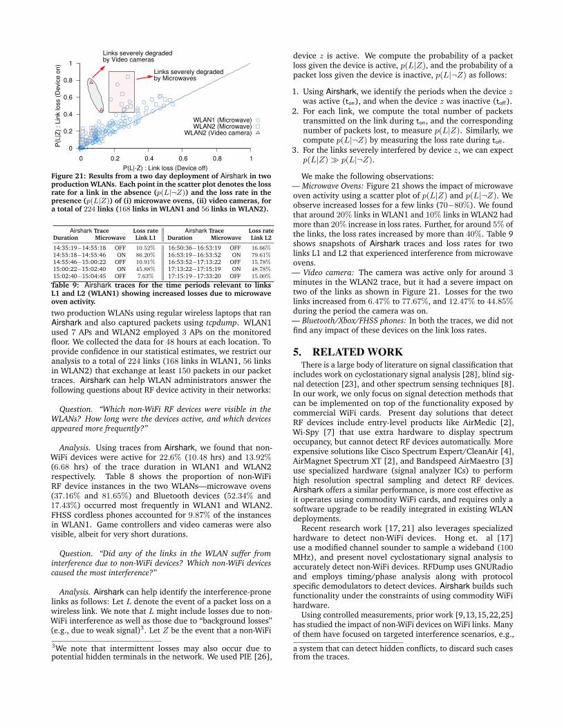
4.1.2 Multiple device detection accuracy

Method. For each run, we chose 2 n 8 random devicesfrom our device set, placed them at random locations andactivated them simultaneously to generate samples at differentRSSI values. We then computed the average detection

00.020.04

Analog Audio Bluetooth FHSSMicrowaveVideo Xbox Zigbee

FP

R

Phone Tx Phone Camera

single device

0

0.02

0.04

FP

R 2/3 devices

0

0.02

0.04F

PR

>=4 devices

Figure 17: False positive rate for different devices.

Location/environment Accuracy False +ves

Indoor offices (floor-to-ceiling walls) 98.47% 0.029%Lab environment (cubicle-style offices) 94.3% 0.067%Apartments (dormitory-style) 96.21% 0.043%

Table 4: Airshark’s performance in different environments.

accuracy at each RSSI. We repeat the experiments for differentcombinations of devices and locations. We note that ourexperiments include the “overlapping signal” cases (§3.4).

Results. Figure 16 shows the detection accuracy for 2, 3, and� 4 device combinations. We observe that even when � 4

devices are activated simultaneously, the average detectionaccuracy is more than 91% for RSSI values as low as �80 dBm.For higher RSSI values (� �60 dBm), the detection accuracywas 96%. For lower RSSI values, in the presence of multipleRF devices, we observed that features like spectral signatures,duty cycles do not perform well, and hence result in reducedaccuracy (§4.2.1). Overall, we find that Airshark is reasonablyaccurate, and as we show in §4.1.6, its performance is close tothat of signal analyzers [3] using custom hardware.

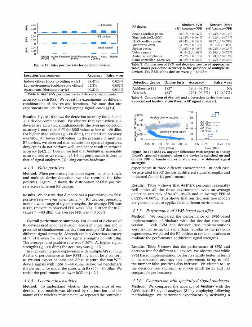
4.1.3 False positives

Method. When performing the above experiments for singleand multiple device detection, we also recorded the falsepositives. Figure 17 shows the distribution of false positiverate across different RF devices.

Results. We observe that Airshark has a particularly low falsepositive rate — even when using � 4 RF devices, operatingunder a wide range of signal strengths, the average FPR was0.39% (maximum observed FPR was 1.3%). Further, for RSSIvalues � �80 dBm, the average FPR was 0.068%.

Overall performance summary. For a total of 8 classes ofRF devices used in our evaluation, across multiple runs and inpresence of simultaneous activity from multiple RF devices atdifferent signal strengths, Airshark exhibits detection accuracyof � 91% even for very low signal strengths of �80 dBm.The average false positive rate was 0.39%. At higher signalstrengths (� �60 dBm) the accuracy was � 96%.

In a typical enterprise deployment with multiple APs runningAirshark, performance at low RSSI might not be a concernas we can expect at least one AP to capture the non-WiFidevice signals with RSSI ��80 dBm. Below, we benchmarkthe performance under the cases with RSSI � �80 dBm. Werevisit the performance at lower RSSI in §4.2.1.

4.1.4 Location insensitivity

Method. To understand whether the peformance of ourdecision tree models was affected by the location and thenature of the wireless environment, we repeated the controlled

RF device Airshark-SVM Airshark-DTree(%) Accuracy/FPR (%)Accuracy/FPR

Analog cordless phone 98.31% / 0.037% 97.73% / 0.012%Bluetooth (ACL/SCO) 92.03% / 0.094% 91.63% / 0.076%FHSS cordless phone 98.44% / 0.052% 96.47% / 0.037%Microwave oven 94.02% / 0.012% 93.16% / 0.06%ZigBee device 97.49% / 0.048% 96.23% / 0.036%Video camera 94.24% / 0.08% 92.70% / 0.072%Audio tx/headphones 92.27% / 0.016% 91.23% / 0.014%Game controller (Xbox/Wii) 90.32% / 0.064% 91.75% / 0.046%

Table 5: Comparison of SVM and decision tree based approaches.Table shows per-device accuracy in the presence of multiple RFdevices. The RSSI of the devices were � �80 dBm.

Detection device Online tests Accuracy False +ves

AirMaestro [3] 1827 1803 (98.7%) NAAirshark 1827 1761 (96.3%) 12 (0.07%)

Table 6: Comparison of Airshark and a detection device that usesa specialized hardware (AirMaestro RF signal analyzer).

0

0.05

0.1

0.15

0.2

0.25

-100 -90 -80 -70 -60 -50 -40

An

gu

lar

diff

. (r

ad

ian

s)

RSSI (dBm)

Analog phone inactive

Analog phone active

0

20

40

60

80

100

-1.5 -0.75 0 0.75 1.5

CD

F

Error (MHz)

-30 dBm-50 dBm-70 dBm-90 dBm

Figure 18: (a) RSSI vs. angular difference with respect to analogphone’s spectral signature when the device is switched on andoff (b) CDF of bandwidth estimation error at different signalstrengths.

experiments in three different environments. In each case,we activated the RF devices at different signal strengths andmeasured Airshark’s performance.

Results. Table 4 shows that Airshark performs reasonablywell under all the three environments with an averagedetection accuracy of 94.3%�98.4% and an average FPR of0.029%�0.067%. This shows that our decision tree modelsare general, and are applicable in different environments.

4.1.5 Performance of SVM-based classifier

Method. We compared the performance of SVM-basedimplementation of Airshark with the decision tree basedversion. Both SVM and decision tree implementationswere trained using the same data. Similar to the previousexperiments, we placed the RF devices at random locations toevaluate the performance at different signal strengths.

Results. Table 5 shows that the performance of SVM anddecision tree for different RF devices. We observe that whileSVM based implementation performs slightly better in termsof the detection accuracy (an improvement of up to 4%),the number false positives also increase. We elected to usethe decision tree approach as it was much faster and hascomparable performance.

4.1.6 Comparison with specialized signal analyzers

Method. We compared the accuracy of Airshark with theAirMaestro RF signal analyzer [3] by employing followingmethodology: we performed experiments by activating a

0 25 50 75

100

0 0.25 0.5 0.75 1

% A

ccu

racy

Normalized Airtime Utilization

Analog (high)Zigbee (high)

Bluetooth (high) 0

25 50 75

100

0 0.25 0.5 0.75 1

% A

ccu

racy

Normalized Airtime Utilization

Analog (low)Zigbee (low)

Bluetooth (low)

Figure 19: Stress testing Airshark with extreme WiFi interference.Detection accuracy is reduced for pulsed transmission devices(e.g., ZigBee), whereas accuracy for frequency hoppers isminimally affected.

Choice of �s �105 dBm �95 dBm �85 dBm

Accuracy (FPR) 97.3% (4.7%) 92.13% (0.041%) 89.24% (0.023%)

Table 7: Effect of different thresholds on Airshark’s performance.

combination of RF devices at different signal strengths andcollected traces from both Airshark and the AirMaestro devicesimultaneously. Table 6 shows the results.

Results. We observe that out of 1827 device instances,AirMaestro was correctly able to detect 1803 (98.7%), whereasAirshark detected 1761 (96.3%) instances. Further, out of66 instances where Airshark failed to identify the device, 48instances had RSSI values of less than �80 dBm and the restinvolved frequency hopping devices with multiple other RFdevices operating simultaneously. We observed a total of12 (0.07%) false positives and these instances occured whenoperating multiple RF devices at low signal strengths.

4.2 MicrobenchmarksAirshark’s detection accuracy is affected by low signal

strengths and increased WiFi interference. Below we investi-gate these scenarios.

4.2.1 Performance under low signal strengths

We now highlight some of the reasons for reduced accuracyat low signal strengths by examining two of the features.

— Spectral signatures. Consider a particular center frequencyand associated bandwidth where we can expect an analogphone to operate. We wish to compute the spectral signatureon this band (based on the received power in the FFT bins)and then measure the angular difference w.r.t. analog phone’sspectral signature for (i) when the analog phone is active atthis center frequency, (ii) when the phone is inactive. ForAirshark to clearly distinguish between these two cases, theremust be a clear separation between the angular differences i.e.,angular difference must be low when the phone is active,and higher when it is inactive. To understand the worstcase performance, we also activate multiple other RF devicesby placing them at random locations. Figure 18(a) showsthat even in the presence of multiple devices, the angulardifference is very low when the phone is operating at higherRSSI. However, when the phone is operating at lower signalstrengths, the angular difference increases, thereby reducingAirshark’s detection accuracy.

—Bandwidth estimation. In each run we activate a randomRF device at a random location and let Airshark compute thebandwidth of the signal. Figure 18(b) shows the error incomputed bandwidth at different RSSI values. We observethat Airshark performs very well at high RSSI values, but thebandwidth estimation error increases at low signal strengths,thereby affecting the detection accuracy.

4.2.2 Performance under extreme interference

0.3

0.6

0.9

1.2

5k 15k 45k 145k

NK

LD

Number of samples

1m3m5m7m

8m10m12m14m

0.3

0.6

0.9

1.2

5k 15k 45k 145k

NK

LD

Number of samples

AudioTxMicrowave

ZigbeeFHSS phone

XBOXBluetooth

Figure 20: NKLD values wrt. to audio transmitter’s pulsedistribution for (a) audio transmitter at different distances (b)different RF devices

Deployment Proportion of RF device instancesMicrowave Bluetooth FHSS Phone Videocam Xbox

WLAN1 37.16% 52.34% 9.87% – 0.6%WLAN2 81.65% 17.43% – 0.917% –

Table 8: Proportion of non-WiFi RF device instances in 2production WLANs. We collected data using Airshark for aduration of 48 hours.

We performed stress tests on Airshark by introducingadditional WiFi interference traffic. We placed a WiFitransmitter close to the Airshark node (distance of 1m) and letit broadcast packets on the same channel as the fixed frequencyRF devices. We changed the WiFi traffic load resultingin different airtime utilizations. We tested the detectionaccuracy of RF devices at HIGH and LOW signal strengths(�50 dBm and �80 dBm respectively). Figure 19 shows theeffect on Airshark’s detection accuracy w.r.t. normalized airtime utilization (air time utilization is maximum, when thetransmitter broadcasts packets at full throughput). Accuracyof high duty devices (analog phone) is affected only in theLOW case, when normalized airtime utilization is close to 1.For devices like ZigBee (fixed frequency, pulsed transmissions),the effect is more severe in the LOW case under increasedairtime utilization. Frequency hopping devices like Bluetooth,however, are not affected because Airshark is able to collectenough pulses from other sub-bands. It is worth pointingout that all the previous experiments were performed inthe presence of regular WiFi traffic and in different wirelessenvironments. We therefore believe that Airshark performsreasonably well under realistic WiFi workloads.

4.2.3 Parameter tuning

We now discuss the empirically established parameters ofour system. Table 7 shows the effect of using different energythresholds. The set up for the experiments was similar to thatin §4.1.2. We observe that while it is possible to improveAirshark’s accuracy at lower RSSI values by lowering thethreshold, this comes at the cost of increased false positives.Increasing the threshold reduces the number of peaks (andhence pulses) detected and reduces the detection accuracy.

We now show the effect of number of samples on the NKLDvalues. Figure 20 (left) shows how the NKLD values convergefor an audio transmitter device (placed at different distances)with the total number of samples processed by Airshark. Wefind that around 15000 samples, the NKLD values convergeto 0.3. Figure 20 (right) compares the NKLD of differentRF devices when using the pulse distribution of the audiotransmitter device as reference. We find that 15000 samplesare sufficient, as NKLD values of 0.3 can be used to indicatethe pulse distribution of the audio transmitter.

4.3 Example uses of AirsharkWe now demonstrate Airshark’s potential through example

applications. We monitored the RF activity on a single floor of

0

0.2

0.4

0.6

0.8

1

0 0.2 0.4 0.6 0.8 1

P(L

|Z)

: L

ink

loss

(D

evi

ce o

n)

P(L|-Z) : Link loss (Device off)

Links severely degraded by Microwaves

Links severely degraded by Video cameras

WLAN1 (Microwave)WLAN2 (Microwave)

WLAN2 (Video camera)

Figure 21: Results from a two day deployment of Airshark in twoproduction WLANs. Each point in the scatter plot denotes the lossrate for a link in the absence (p(L|¬Z)) and the loss rate in thepresence (p(L|Z)) of (i) microwave ovens, (ii) video cameras, fora total of 224 links (168 links in WLAN1 and 56 links in WLAN2).

Airshark Trace Loss rate Airshark Trace Loss rateDuration Microwave Link L1 Duration Microwave Link L2

14:35:19�14:55:18 OFF 10.52% 16:50:36�16:53:19 OFF 16.66%14:55:18�14:55:46 ON 86.20% 16:53:19�16:53:52 ON 79.61%14:55:46�15:00:22 OFF 10.91% 16:53:52�17:13:22 OFF 15.78%15:00:22�15:02:40 ON 45.88% 17:13:22�17:15:19 ON 48.78%15:02:40�15:04:45 OFF 7.63% 17:15:19�17:33:20 OFF 15.00%

Table 9: Airshark traces for the time periods relevant to linksL1 and L2 (WLAN1) showing increased losses due to microwaveoven activity.

two production WLANs using regular wireless laptops that ranAirshark and also captured packets using tcpdump. WLAN1used 7 APs and WLAN2 employed 3 APs on the monitoredfloor. We collected the data for 48 hours at each location. Toprovide confidence in our statistical estimates, we restrict ouranalysis to a total of 224 links (168 links in WLAN1, 56 linksin WLAN2) that exchange at least 150 packets in our packettraces. Airshark can help WLAN administrators answer thefollowing questions about RF device activity in their networks:

Question. “Which non-WiFi RF devices were visible in theWLANs? How long were the devices active, and which devicesappeared more frequently?”

Analysis. Using traces from Airshark, we found that non-WiFi devices were active for 22.6% (10.48 hrs) and 13.92%(6.68 hrs) of the trace duration in WLAN1 and WLAN2respectively. Table 8 shows the proportion of non-WiFiRF device instances in the two WLANs—microwave ovens(37.16% and 81.65%) and Bluetooth devices (52.34% and17.43%) occurred most frequently in WLAN1 and WLAN2.FHSS cordless phones accounted for 9.87% of the instancesin WLAN1. Game controllers and video cameras were alsovisible, albeit for very short durations.

Question. “Did any of the links in the WLAN suffer frominterference due to non-WiFi devices? Which non-WiFi devicescaused the most interference?”

Analysis. Airshark can help identify the interference-pronelinks as follows: Let L denote the event of a packet loss on awireless link. We note that L might include losses due to non-WiFi interference as well as those due to “background losses”(e.g., due to weak signal)3. Let Z be the event that a non-WiFi

3We note that intermittent losses may also occur due topotential hidden terminals in the network. We used PIE [26],

device z is active. We compute the probability of a packetloss given the device is active, p(L|Z), and the probability of apacket loss given the device is inactive, p(L|¬Z) as follows:

1. Using Airshark, we identify the periods when the device zwas active (t

on

), and when the device z was inactive (to↵

).2. For each link, we compute the total number of packets

transmitted on the link during ton

, and the correspondingnumber of packets lost, to measure p(L|Z). Similarly, wecompute p(L|¬Z) by measuring the loss rate during t

o↵

.3. For the links severely interfered by device z, we can expect

p(L|Z) � p(L|¬Z).

We make the following observations:— Microwave Ovens: Figure 21 shows the impact of microwaveoven activity using a scatter plot of p(L|Z) and p(L|¬Z). Weobserve increased losses for a few links (70�80%). We foundthat around 20% links in WLAN1 and 10% links in WLAN2 hadmore than 20% increase in loss rates. Further, for around 5% ofthe links, the loss rates increased by more than 40%. Table 9shows snapshots of Airshark traces and loss rates for twolinks L1 and L2 that experienced interference from microwaveovens.— Video camera: The camera was active only for around 3

minutes in the WLAN2 trace, but it had a severe impact ontwo of the links as shown in Figure 21. Losses for the twolinks increased from 6.47% to 77.67%, and 12.47% to 44.85%during the period the camera was on.— Bluetooth/Xbox/FHSS phones: In both the traces, we did notfind any impact of these devices on the link loss rates.

5. RELATED WORKThere is a large body of literature on signal classification that

includes work on cyclostationary signal analysis [28], blind sig-nal detection [23], and other spectrum sensing techniques [8].In our work, we only focus on signal detection methods thatcan be implemented on top of the functionality exposed bycommercial WiFi cards. Present day solutions that detectRF devices include entry-level products like AirMedic [2],Wi-Spy [7] that use extra hardware to display spectrumoccupancy, but cannot detect RF devices automatically. Moreexpensive solutions like Cisco Spectrum Expert/CleanAir [4],AirMagnet Spectrum XT [2], and Bandspeed AirMaestro [3]use specialized hardware (signal analyzer ICs) to performhigh resolution spectral sampling and detect RF devices.Airshark offers a similar performance, is more cost effective asit operates using commodity WiFi cards, and requires only asoftware upgrade to be readily integrated in existing WLANdeployments.

Recent research work [17, 21] also leverages specializedhardware to detect non-WiFi devices. Hong et. al [17]use a modified channel sounder to sample a wideband (100MHz), and present novel cyclostationary signal analysis toaccurately detect non-WiFi devices. RFDump uses GNURadioand employs timing/phase analysis along with protocolspecific demodulators to detect devices. Airshark builds suchfunctionality under the constraints of using commodity WiFihardware.

Using controlled measurements, prior work [9,13,15,22,25]has studied the impact of non-WiFi devices on WiFi links. Manyof them have focused on targeted interference scenarios, e.g.,

a system that can detect hidden conflicts, to discard such casesfrom the traces.

between Bluetooth-WiFi [13] or ZigBee-WiFi [22, 25], andproposed mechanisms for co-existence [10,18]. Similar to [9,15], we consider the general problem of non-WiFi interference,but specifically, we focus on the problem of making existingWiFi links better aware of non-WiFi RF devices, thereby pavingthe way for corrective actions that can be implemented intoday’s networks. Further, our mechanism is complementaryto the above solutions, and can be used in conjunction to moreeffectively tackle non-WiFi interference.

6. CONCLUSIONIn this work, we first motivated the need to detect non-

WiFi RF devices by characterizing their prevalence in typicalenvironments. We then presented Airshark, a system thatcan detect the non-WiFi devices using only the functionalityprovided by commodity WiFi cards. Airshark extracts uniquefeatures using energy samples from a WiFi card and presentsa generic, and extensible framework to accurately detectmultiple non-WiFi devices, while maintaining a low falsepositive rate. We also found its performance to be comparableto a commercial signal analyzer. Through a deployment in twoproduction WLANs, we demonstrated Airshark’s potential inunderstanding non-WiFi interference issues.

We envision embedding Airshark in commodity wirelessAPs that opens up numerous other possibilities. WLANadministrators can monitor RF device activity across thenetwork without deploying additional hardware. APs canalso employ real-time, non-WiFi interference mitigationmechanisms based on the input from Airshark (e.g., deviceRSSI/channel). Another application is to physically locatethe RF interferer. Localization can be done by correlatingthe device transmissions across samples from multiple Air-

shark nodes and then using triangulation methods.

AcknowledgementsWe thank Vishnu Katreddy for help with some of the measure-ments carried out in this paper. We would also like to thankthe anonymous reviewers, whose comments helped bring thepaper into its final form. Shravan Rayanchu, Ashish Patro,and Suman Banerjee have been supported in part by the USNational Science Foundation through awards CNS-1059306,CNS-0855201, CNS-0747177, CNS-0916955, CNS-1040648,and CNS-1064944.

7. REFERENCES[1] Agilent spectrum analyzers (signal analyzers).

http://www.agilent.com/.[2] AirMagnet AirMedic and Spectrum XT.

www.airmagnet.net/products.[3] Bandspeed AirMaestro spectrum analysis solution.

http://www.bandspeed.com/.[4] Cisco Spectrum Expert.

http://www.cisco.com/en/US/products/ps9393/index.html.[5] LIBSVM: A Library for Support Vector Machines.

http://www.csie.ntu.edu.tw/ cjlin/libsvm/.[6] The WEKA data mining software: an update. ACM

SIGKDD Explorations Newsletter.[7] Wi-Spy spectrum analyzer. www.metageek.net.[8] I. F. Akyildiz, W.-Y. Lee, M. C. Vuran, and S. Mohanty.

Next generation/dynamic spectrum access/cognitiveradio wireless networks: a survey. Comput. Netw., 2006.

[9] A. Baid, S. Mathur, I. Seskar, T. Singh, S. Jain,D. Raychaudhuri, S. Paul, and A. Das. Spectrum MRI:Towards diagnosis of multi-radio interference in theunlicensed band. In IEEE WCNC 2011.

[10] M. C.-H. Chek and Y.-K. Kwok. Design and evaluation ofpractical coexistence management schemes forBluetooth and IEEE 802.11b systems. In ComputerNetworks,’07.

[11] P. Du, W. A. Kibbe, and S. M. Lin. Improved peakdetection in mass spectrum by incorporating continuouswavelet transform-based pattern matching. InBioinformatics’06.

[12] G. Palshikar. Simple algorithms for peak detection intime-series, trddc technical report’09. In TechnicalReport, TRDDC.

[13] N. Golmie, N. Chevrollier, and O. Rebala. Bluetooth andWLAN coexistence: Challenges and solutions. IEEEWireless Communications Magazine’03.

[14] R. C. Gonzalez and R. E. Woods. Digital imageprocessing, 3rd ed. 2006.

[15] R. Gummadi, D. Wetherall, B. Greenstein, and S. Seshan.Understanding and mitigating the impact of RFinterference on 802.11 networks. In SIGCOMM ’07.

[16] K. Harmer, G. Howells, W. Sheng, M. Fairhurst, andF. Deravi. A peak-trough detection algorithm based onmomentum. In CISP’08.

[17] S. Hong and S. Katti. Wispy: Knowing your RFneighborhood. In ACM SIGCOMM 2011.

[18] X. Jing, S. Anandaraman, M. Ergin, I. Seskar, andD. Raychaudhuri. Distributed coordination schemes formulti-radio co-existence in dense spectrumenvironments. In IEEE DySpan ’08.

[19] A. Kamerman and N. Erkogevi. Microwave oveninterference on wireless Lans operating in the 2.4 GHzISM band. In PIMRC’97.

[20] Kullback, S. Information theory and statistics, 1959.[21] K. Lakshminarayanan, S. Sapra, S. Seshan, and

P. Steenkiste. RFDump: an architecture for monitoringthe wireless ether. In CoNext’09.

[22] C.-J. M. Liang, N. B. Priyantha, J. Liu, and A. Terzis.Surviving Wi-Fi interference in low power zigbeenetworks. In ACM SenSys’10.

[23] O. Zakaria. Blind signal detection and identification overthe 2.4 GHz ISM band for cognitive radio. In MS ThesisUSF’09.

[24] J. R. Quinlan. C4.5: programs for machine learning.Morgan Kaufmann Publishers Inc., 1993.

[25] S. Y. Shin, J. S. Kang, and H. S. Park. Packet error rateanalysis of zigbee under wlan and bluetoothinterferences. In IEEE Trans. Wireless Comm.’06.

[26] V. Shrivastava, S. Rayanchu, S. Banerjee, andK. Papagiannaki. PIE in the Sky: online passiveinterference estimation for enterprise WLANs. InNSDI’11.

[27] T. M. Taher, A. Z. Al-Banna, D. R. Ucci, and J. L.LoCicero. Characterization of an unintentional Wi-Fiinterference device-the residential microwave oven. InMilcom’06.

[28] W. Gardner. Exploitation of spectral redundancy incyclostationary signals. In IEEE Signal ProcessingMagazine’91.