detailed comparison of dns to pse for oblique … comparison of dns to pse for ... nism if it can...

Detailed Comparison of DNS to PSE for Oblique

Breakdown at Mach 3 (Abstract)

Christian S. J. Mayer∗ and Hermann F. Fasel†

The University of Arizona, Tucson, AZ 85721

Meelan Choudhari‡ and Chau-Lyan Chang‡

NASA Langley Research Center, Hampton, VA 23681

A pair of oblique waves at low amplitudes is introduced in a supersonic flat-plate bound-ary layer. Their downstream development and the concomitant process of laminar toturbulent transition is then investigated numerically using Direct Numerical Simulations(DNS) and Parabolized Stability Equations (PSE). This abstract is the last part of an ex-tensive study of the complete transition process initiated by oblique breakdown at Mach3. In contrast to the previous simulations, the symmetry condition in the spanwise direc-tion is removed for the simulation presented in this abstract. By removing the symmetrycondition, we are able to confirm that the flow is indeed symmetric over the entire compu-tational domain. Asymmetric modes grow in the streamwise direction but reach only smallamplitude values at the outflow. Furthermore, this abstract discusses new time-averageddata from our previous simulation CASE 3 and compares PSE data obtained from NASA’sLASTRAC code to DNS results.

I. Introduction

To date, the most dominant nonlinear mechanism that eventually transitions a laminar, supersonic bound-ary layer to turbulence is still unknown. Knowledge of the relevant nonlinear mechanisms is however manda-tory for the accurate determination of transition onset. Previous investigations1–3 of the nonlinear transitionregime discovered two main nonlinear mechanisms, “oblique breakdown” and “asymmetric subharmonic res-onance”. Recently, a series of numerical studies4–9 using direct numerical simulations (DNS) focused onseveral unresolved issues related to both mechanisms. In the first part of these studies,4, 5 the authors wereable to identify oblique breakdown in the experiments by Kosinov and his co-workers,2, 10–12 who investigatedasymmetric subharmonic resonance initiated by a wave train in a flat-plate boundary layer at Mach 2. Theidentification of oblique breakdown in these experiments is of great importance since a detailed, experimentalstudy of this mechanism has not been performed yet.

The second part of these studies8 addressed the question whether oblique breakdown or asymmetricsubharmonic resonance, is a stronger nonlinear breakdown mechanism in supersonic boundary layers. Inorder to answer this question, Mayer et al.8 investigated the early nonlinear transition regime initiated bya broad disturbance spectrum on a cone at Mach 3.5. To excite a wide range of disturbance waves, awave packet was generated by a pulse through a hole on the cone surface. The disturbance spectrum inthe frequency-azimuthal mode number plane of the wave packet exhibited traces of oblique breakdown andnew features that could be explained with new resonance triads that are composed of three boundary layermodes with three different disturbance frequencies. Furthermore, it was shown that asymmetric subharmonicresonance is a limiting case of these new resonance triads with both secondary waves having subharmonicfrequency and that oblique breakdown might be another limiting case with one secondary wave havingzero frequency. Moreover, theoretical considerations suggested that oblique breakdown might be a stronger

∗Research Assistant, Dept. of Aerospace & Mechanical Engineering, Tucson, AZ 85721, AIAA member†Professor, Dept. of Aerospace & Mechanical Engineering, Tucson, AZ 85721, AIAA member‡Aerospace Technologist, Computational Aerosciences Branch, Associate Fellow AIAA

1 of 9

American Institute of Aeronautics and Astronautics

https://ntrs.nasa.gov/search.jsp?R=20100024514 2018-06-29T09:27:16+00:00Z

nonlinear transition mechanism for two-dimensional boundary layers at supersonic speeds than any otherresonance triad.

A nonlinear transition mechanism, however, can only be considered to be an important physical mecha-nism if it can initiate the entire transition process of a laminar boundary layer to turbulence. This issue wasaddressed by the final part of the series of numerical studies,6, 7, 9 where the entire transition path of obliquebreakdown for a flat-plate boundary layer at Mach 3 was simulated. The DNS in these references, however,had one shortcoming, that is, the flow was assumed to be symmetric in the spanwise direction to reducecomputational costs. In order to ensure that this assumption is indeed valid, a new DNS has been conductedin which the artificial symmetry restriction was removed. As a first part, the final conference paper willshow results from this simulation and additional longer time-average from the original symmetric simulationof Mayer et al.7 (CASE 3). Simulations of the complete transition process as in Mayer et al.7 provide avaluable and extensive database that can be utilized for the validation of several different engineering toolsacross the various stages of transition. The second part of the final conference paper will therefore compareDNS results of the early and late nonlinear stages to data from NASA’s LASTRAC code. This code is basedon the nonlinear parabolized stability equations.

II. Simulation Setup for the DNS

The simulation setup for the DNS in this abstract follows Mayer et al.6, 7 Supersonic flow at Mach 3over a flat plate is investigated numerically using spatial DNS. The physical conditions of the simulationsmatch the Princeton wind tunnel conditions:13 the unit Reynolds number formed with the free-streamvelocity and free-stream viscosity at the inflow was Re = 2.181 × 106m−1 and the free-stream temperatureis T ∗

∞= 103.6K. In the following, details of the computational setup are given and then information on

governing equations, boundary conditions, disturbance generation and numerical method are repeated fromMayer et al.6, 7 for completeness and convenience of the reader.

A. Computational Setup

The main parameters for both DNS discussed in this abstract are summarized in table ??. The samenomenclature as in Mayer et al.6, 7 is employed. Hence, CASE 3 denotes the main case from the olderreferences while CASE 7 is the newest simulation. The overall resolution is exactly the same for both cases.The grid is clustered in the streamwise direction using a fifth-order polynomial and in the wall-normaldirection using a third-order polynomial. The computational grid in physical space consists of a total ofabout 212 million grid points for CASE 3 and 324 million grid points for CASE 7.

Table 1. Main simulation parameters that differ between cases.

Parameter Unit CASE 3 CASE 7

Domain size:

xL [m] 1.145 1.050

yH [m] 0.030 0.030

Grid size:

nx [−] 2757 2101

ny [−] 301 301

K [−] 128 256

nz [−] 255 512

nx × ny × nz [−] 211.6E6 323.8E6

Grid resolution (at outflow):

points per λ[1,1]x [−] ∼ 440 ∼ 440

FFT’s:

Symmetry in z? [−] yes no

The inflow of the domain for both cases is located at x∗

0 = 0.258m downstream of the leading edge

2 of 9


of the plate, whereas the outflow ranges from approximately 13.1 (CASE 7) to 14.5 (CASE 3) streamwisewavelengths λx of the oblique fundamental disturbance waves in the linear regime. The domain height ischosen as y∗

H = 0.030m ≈ 5 boundary layer thicknesses δ (laminar) at the outflow, such that even with thelarge increase in boundary layer thickness caused by the transition process no turbulent flow structures reachthe free-stream boundary.

Time-harmonic disturbances with a fundamental frequency of about f∗ = 6.36kHz (F = 3 × 10−5) areintroduced through a blowing and suction slot located between x∗

1 = 0.394m and x∗

2 = 0.452m (x2−x1 ≈ λx).A discrete wave pair of instability waves with equal but opposite wave angle is excited for all cases. Thespanwise wavenumber of β∗ = 211.52m−1 for the oblique wave pair is chosen such that the generatedinstability waves experience strong amplification as predicted by LST throughout the entire computationaldomain. This spanwise wavenumber determines also the domain width of all simulations, i.e. z∗W = λ∗

z =2π/β∗ = 0.03m.

B. Governing Equations

The physical problem is governed by the conservation of mass, momentum and total energy with appropriateboundary and initial conditions. The fluid was considered to be a perfect gas with constant specific heatcoefficients. The equations were cast in non-dimensional form using an arbitrary reference length (the platelength L∗ = 0.7239m) and the free-stream values of the flow quantities at the inflow boundary:

∂ρ

∂t+

∂

∂xj

(ρuj) = 0 , (1)

∂ρui

∂t+

∂

∂xj

(ρuiuj + δijp − τij) = 0 , (2)

∂Et

∂t+

∂

∂xj

([Et + p]uj − uiτij + qj) = 0 . (3)

The total energy Et and the viscous stress τij are defined as:

Et = ρ

(T

κ(κ − 1)Ma2 +ukuk

2

), τij =

µ

Re

(∂ui

∂xj

+∂uj

∂xi

−2

3δij

∂uk

∂xk

). (4)

The pressure p is computed using the equation of state and the heat flux qi is obtained from Fourier’s law:

p =ρT

κMa2 , qi = −µ

(κ − 1)Ma2RePr

∂T

∂xi

, (5)

with κ = 1.4 and Pr = 0.71. The viscosity is calculated using Sutherland’s law

µ(T ) = T3

2

1 + CT∗

∞

T + CT∗

∞

, (6)

with C = 110.4K.

C. Boundary Conditions

At the inflow, the conservative quantities ρ, ρui and Et, obtained from the similarity solution of a compressibleflat-plate boundary layer, are specified. The outflow is treated with a buffer domain technique14 to avoidreflections of disturbance waves. The buffer domain starts at x3 and ends slightly upstream of xL with alength of xL−x3 ∼ 0.5λx for all cases. At the free-stream boundary, all total flow quantities are separated intobase-flow and disturbance quantities. For the base-flow quantities, a homogeneous von Neumann condition isapplied whereas for the disturbance quantities an exponential decay condition is employed that was derivedfor compressible flow using linear stability considerations.15 In the lateral direction, periodicity is assumed.At the wall, the no-slip and no-penetration conditions are used except for the disturbance slot (see below). Inaddition, for the base flow, the wall temperature is set to the adiabatic wall temperature of the correspondinglaminar flow, i.e. the initial condition, whereas temperature fluctuations are assumed to vanish.

3 of 9


D. Disturbance Generation

The flow is forced over the disturbance slot by prescribing a time-harmonic function for the fundamentalspanwise Fourier mode of the v-velocity. During the startup of the simulation, the forcing amplitude A(β, t)is ramped up in time over one disturbance period. The velocity distribution vp over the blowing and suctionslot has the shape of a dipole and it is represented by a fifth-order polynomial that is smooth everywhereincluding at the end points:

v (xp, y = 0, β, t) = A (β, t) vp (xp) cos (−ωt + θp (β)) . (7)

xp was defined as

xp =2x − (x2 + x1)

x2 − x1, −1 ≤ xp ≤ 1 . (8)

E. Numerical Method

The governing equations are integrated in time by employing a fourth-order Runge–Kutta scheme. Thespatial derivatives are discretized using formally fourth-order split-finite differences in the streamwise andwall-normal directions.16 The spanwise direction is assumed to be periodic and therefore transformed intospectral space using Fast Fourier transforms. Moreover, the spanwise discretization is pseudo-spectral, i.e.all nonlinear terms in the governing equations are computed in physical space and then transformed backinto spectral space. Two options are implemented for the Fourier Transformations: (i) All flow variables (i.e.u-velocity, v-velocity, etc.) are assumed to be symmetric to the centerline, except for the spanwise velocityw, which is antisymmetric. Symmetric quantities are then transformed into Fourier space using a Fouriercosine transformation and antisymmetric variables (w) are transformed by a Fourier sine transformation.Thus, only one-half spanwise wave length λz has to be computed for this configuration. (ii) No symmetry isassumed and therefore, all variables are transformed using a full Fourier transformation. This option requiresthe computation of the entire wave length λz in spanwise direction.

The Fourier transformations are based on the VFFTPK library, which can be downloaded from netlib(http://www.netlib.org/vfftpack/). According to this library and its implementation in the Navier–Stokescode, a Fourier cosine transformation into spectral space and its back transformation into physical space aregiven by

physical→spectral:

φck = F (φ)c

k ∼1

2(nz − 1)

[φc

0 + 2

nz−1∑

l=1

φcl cos

(πkl

nz − 1

)](9a)

spectral→physical:

φcl = F

−1(φ)c

l∼ φc

0 + 2

K−1∑

k=1

φckcos

(πkl

nz − 1

)(9b)

for k = 0, ..., K − 1 and l = 0, ...., nz − 1, respectively. φck represent the Fourier amplitudes for mode k.

Moreover, nz indicates the number of grid points used for resolving the spanwise direction in physical spaceover the interval [0, (nz − 1)∆z] with

∆z =λz

2(nz − 1)(10)

and K represents the number of modes in Fourier space (for the simulations nz = 2K − 1).The Fourier sine transformation to spectral space and its back transformation into physical space are as

follows


φsk = F (φ)

s

k ∼ −1

(nz − 1)

nz−1∑

l=1

φsl sin

(πkl

nz − 1

)(11a)


φsl = F−1

(φ)s

l∼ −2

K−1∑

k=1

φsksin

(πkl

nz − 1

)(11b)

4 of 9


for k = 0, ..., K − 1 and l = 0, ...., nz − 1, respectively.In contrast to a symmetric simulation where only one-half of the spanwise wave length has to be calcu-

lated, an asymmetric simulation requires the entire spanwise wave length as computational domain. Hence,for symmetric simulations nz represents the number of grid points in one-half wave length, whereas forasymmetric simulations, this number depicts the grid points in one full spanwise wave length. In this case,the grid spacing in spanwise direction is therefore obtained from

∆z =λz

(nz − 1). (12)

The full Fourier transformation for an asymmetric simulation is implemented according to


φ0 ∼1

2nz

nz−1∑

l=0

φl (13a)

φck ∼

1

nz

nz−1∑

l=0

φl cos

(2πkl

nz

)(13b)

φsk ∼

1

nz

nz−1∑

l=0

φl sin

(2πkl

nz

)(13c)


φl ∼ φ0 +K−1∑

k=1

[φc

kcos

(2πkl

nz

)+ φs

ksin

(2πkl

nz

)](13d)

with k = 0, ..., K − 1 and l = 0, ...., nz − 1. As for the symmetric case, K denotes the number of Fouriermodes. The entire storage space for the Fourier modes is however 2K − 1 since the cosine modes and thesine modes have to be stored separately. More details on the numerical method as well as validation casescan be found in the theses of Harris16 and von Terzi.17

III. Results and Discussion

This section discusses some preliminary results. In order to confirm that CASE 3 from Mayer et al.7

represents a valuable database for the validation of different engineering tools across the various stagesof transition one remaining issue has to be clarified. In CASE 3, the spanwise direction was assumed tobe symmetric since so far in the literature, oblique breakdown has always been initiated by two symmetric,oblique, first-mode type instability waves. It is, however, not straight forward to determine if this assumptionis indeed justified. Hence, a final simulation where the symmetry restriction is removed is presented insection III.A. Furthermore, this section also shows some results from CASE 3 that are averaged over alonger time interval. The final section (section III.B) provides a preliminary comparison of PSE resultsobtained from NASA’s LASTRAC code to CASE 3 for the early nonlinear transition regime of obliquebreakdown.

A. New DNS results

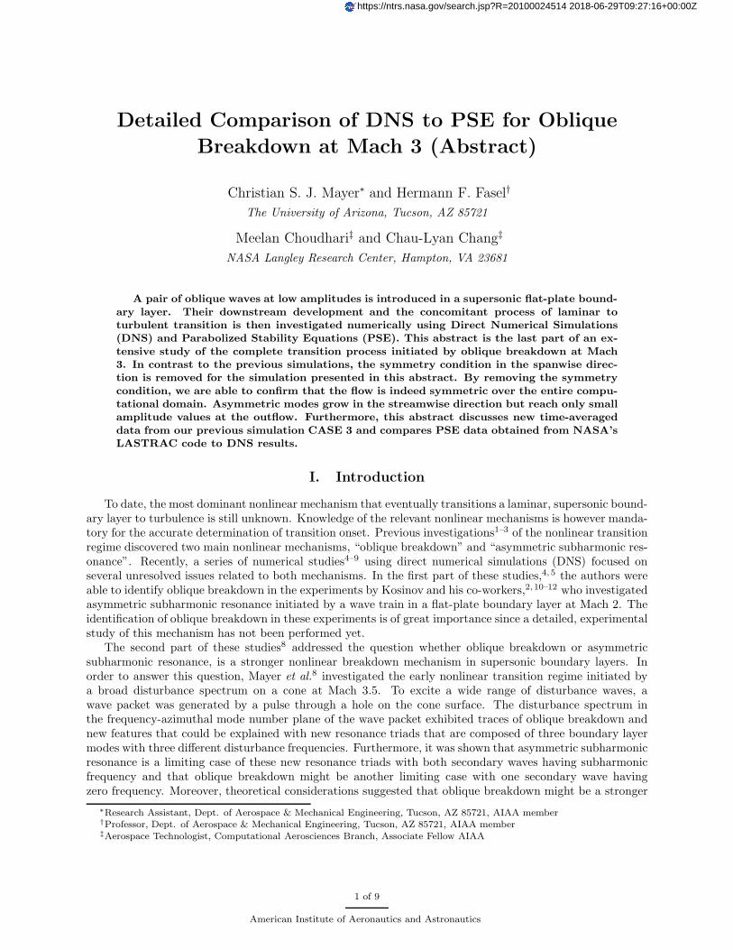
The first two figures show results from the new simulation CASE 7. Since there is no symmetry condition inthe spanwise direction, the computational domain for CASE 7 is doubled in this direction (see also Table 1and section II.E). The influence of asymmetric modes on oblique breakdown initiated by two oblique waveswith exactly the same amplitude and phase is limited since these modes are only generated by the round-offerror of the calculation. In CASE 3 from Mayer et al.,7 the streamwise position of the final breakup intosmall-scale structures denotes the location where all modes with frequency unequal to integer multiples ofthe forcing frequency are strongly amplified. In CASE 7, a similar behavior can be observed. At exactlythe same streamwise position (where the breakup into small-scale structures occurs) the asymmetric modesstart to be amplified as illustrated by figure 1a. This figure shows the streamwise velocity disturbance of thefirst higher Fourier mode in the spanwise direction for the sine and cosine modes. In CASE 3, only cosine

5 of 9


x*, m0.80 0.82 0.84 0.86 0.88 0.90 0.92 0.94 0.96

y*, m

0.02.0

*10-2

x*, m0.80 0.82 0.84 0.86 0.88 0.90 0.92 0.94 0.96

y*, m

0.02.0

*10-2

(a)

(b)

Figure 1. Contours of streamwise velocity u obtained from CASE 7 for the first higher Fourier mode in thespanwise direction: (a) sine mode, (b) cosine mode.

modes were calculated for the streamwise velocity because of symmetry and all sine modes were set to zero.Hence, the amplitude values of the sine mode in figure 1a provide a measure for the magnitude of asymmetryin CASE 7. Since the sine mode in figure 1a is more than 10 orders of magnitude smaller than the cosinemode, CASE 7 remains symmetric even after the breakup into small-scale structures. It is however clearlyvisible that the asymmetric modes are strongly amplified downstream of this position and will eventuallyreach high amplitude values in the turbulent region.

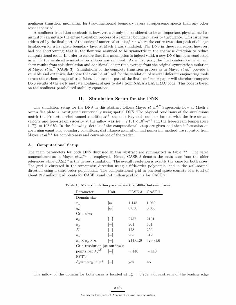
The results from figure 1 corroborate that the symmetry assumption in CASE 3 is justified. Thus, forthe rest of this section, we concentrate on CASE 3. The time average in Mayer et al.7 is calculated over only12 forcing periods. If this interval length for the time average is sufficient, is depicted in figure 2.

0 5 10 15 20 25 30t/Tforcing

0.0028

0.0029

0.0030

0.0031

c f

x*=1.051m

x*=1.087m

x*=1.104m

Figure 2. Skin-friction coefficient for CASE 3 as a function of interval length for time-averaging indicated bythe number of forcing periods Tforcing at three different streamwise positions.

Figure 2 demonstrates the skin-friction coefficient as a function of the interval length for the time averageat three different streamwise positions. For the first two positions, the skin-friction coefficient does not changesignificantly when the interval length for the time average is increased. At the last position (x∗ = 1.104m),however, a longer time average is required. A similar conclusion can be drawn from figure 3, which illustratesthe streamwise distribution of selected mean-flow properties from CASE 3 for two different time averages.The curves with 12 forcing periods as time-average interval are very close to the curves with 25.75 forcingperiods.

As can be seen in figures 2 and 3, the increase in interval length for the time average does not strongly

6 of 9


0.3 0.4 0.5 0.6 0.7 0.8 0.9 1.0 1.1x

*, m

0.000

0.001

0.002

0.003

0.004

c f

Guarini et al. (M=2.5)Maeder et al. (M=3)CASE 3 (12Tforcing)

CASE 3 (25.75Tforcing)

laminar ICWhite (1991)

(a)

0.3 0.4 0.5 0.6 0.7 0.8 0.9 1.0 1.1x

*, m

0

1000

2000

3000

Re Θ



laminar IC

(b)

Figure 3. Streamwise development of selected mean-flow properties from CASE 3 in comparison to differentvalues published in the literature for turbulent supersonic flow18,19 and theoretical models:20 (a) skin-frictioncoefficient cf , (b) Reynolds number based on momentum thickness Θ.

alter the mean values for CASE 3. However, the impact on fluctuation quantities, as for example the r.m.s.values, will be more pronounced. Hence, the final paper will discuss in more detail fluctuation quantitiesobtained from several different averaging intervals at different streamwise positions. Moreover, the finalpaper will also give a more detailed discussion of CASE 7.

B. PSE Comparison

For this abstract, only a preliminary comparison between PSE results and DNS data is provided. Figure 4shows the streamwise development of wall-normal maximum in streamwise velocity disturbance u′ for selectedFourier modes. Symbols represent PSE results and lines DNS data. For mode [1, 1], the agreement betweenPSE and DNS is excellent while for the other modes a discrepancy is visible. This discrepancy is due to thedifferent disturbance generation in both methods. Note that the notation [h, k] is used to identify a particularwave according to its frequency h and its spanwise wavenumber k. h denotes multiples of the fundamentalfrequency f∗ = 6.36kHz and k multiples of the smallest spanwise wavenumber β∗ = 211.52m−1. For thefinal paper, a detailed PSE study will be presented, in which the influence of the forcing method will beaddressed.

IV. Conclusions and Future Work

Transition to turbulence via the oblique breakdown mechanism was investigated for a supersonic flat-plateboundary layer at Mach 3. Our previous studies of the same case focused on the detailed documentationof the different transition stages and demonstrated that oblique breakdown can lead to a fully developedturbulent boundary layer. In these studies, however, the flow was assumed to be symmetric in the spanwisedirection. The verification of that assumption was an important part of the results presented in this abstract.To that end, a new simulation without the assumption of spanwise symmetry was performed. The final paperwill provide a detailed discussion on this subject. Furthermore, new time-averaged data from CASE 3 ofour previous study was shown. In the final paper, the impact of the time-averaging length on fluctuationstatistics will be illustrated. Finally, the full paper will provide a detailed comparison of our DNS data toPSE results from NASA’s LASTRAC code.

7 of 9


Figure 4. Streamwise development of wall-normal maximum in streamwise velocity disturbance u′ for selected

Fourier modes: lines DNS, symbols PSE.

Acknowledgments

This work is funded by the Air Force Office for Scientific Research under grant FA9550-08-1-0211 withDr. John Schmisseur serving as program manager. The computer hours and the technical support providedby NASA Ames are greatly acknowledged.

References

1Fasel, H., Thumm, A., and Bestek, H., “Direct Numerical Simulation of Transition in Supersonic Boundary Layer:

Oblique Breakdown,” Transitional and Turbulent Compressible Flows, edited by L. D. Kral and T. A. Zang, No. 151 in FED,

ASME, 1993, pp. 77–92.2Kosinov, A. D., Semionov, N. V., Shevelkov, S. G., and Zinin, O. I., “Experiments on the Nonlinear Instability of

Supersonic Boundary Layers,” Nonlinear Instability of Nonparallel Flows, edited by D. T. Valentine, S. P. Lin, and W. R. C.

Philips, Springer, 1994, pp. 196–205.3Corke, T. C., Cavalieri, D. A., and Matlis, E., “Boundary-Layer Instability on Sharp Cone at Mach 3.5 with Controlled

Input,” AIAA J., Vol. 40, No. 5, 2002, pp. 1015–1018.4Mayer, C. S. J., Wernz, S., and Fasel, H. F., “Investigation of Oblique Breakdown in a Supersonic Boundary Layer at

Mach 2 Using DNS,” AIAA-2007-0949, 2007.5Mayer, C. S. J. and Fasel, H. F., “Investigation of Asymmetric Subharmonic Resonance in a Supersonic Boundary Layer

at Mach 2 Using DNS,” AIAA-2008-0591, 2008.6Mayer, C. S. J., von Terzi, D. A., and Fasel, H. F., “DNS of Complete Transition to Turbulence Via Oblique Breakdown

at Mach 3,” AIAA-2008-4398, 2008.7Mayer, C. S. J., von Terzi, D. A., and Fasel, H. F., “DNS of Complete Transition to Turbulence Via Oblique Breakdown

at Mach 3: Part. II,” AIAA-2009-3558, 2009.8Mayer, C. S. J., Laible, A. C., and Fasel, H. F., “Numerical Investigation of Transition initiated by a Wave Packet on a

Cone at Mach 3.5,” AIAA-2009-3809, 2009.9von Terzi, D. A., Mayer, C. S. J., and Fasel, H. F., “The Late Nonlinear Stage of Oblique Breakdown to Turbulence in

a Supersonic Boundary Layer,” Laminar-Turbulent Transition, Springer, 2009, in press.10Kosinov, A. D., Semionov, N. V., and Shevelkov, S. G., “Investigation of Supersonic Boundary Layer Stability and

Transition Using Controlled Disturbances,” Methods of Aerophysical Research, edited by A. M. Kharitonov, Vol. 2, 1994, pp.

159–166.11Ermolaev, Y. G., Kosinov, A. D., and Semionov, N. V., “Experimental Investigation of Laminar-Turbulent Transition Pro-

cess in Supersonic Boundary Layer Using Controlled Disturbances,” Nonlinear Instability and Transition in Three-Dimensional

Boundary Layers, edited by P. W. Duck and P. Hall, Kluwer Academic Publishers, 1996, pp. 17–26.12Kosinov, A. D., Maslov, A. A., and Semionov, N. V., “An Experimental Study of Generation of Unstable Disturbances

on the Leading Edge of a Plate at M=2,” J. Appl. Mech. Tech. Phys., Vol. 38, No. 1, 1997, pp. 45–50.13Graziosi, P. and Brown, G. L., “Experiments on Stability and Transition at Mach 3,” J. Fluid Mech., Vol. 472, 2002,

pp. 83–124.

8 of 9


14Meitz, H. and Fasel, H. F., “A Compact-Difference Scheme for the Navier-Stokes Equations in Vorticity-Velocity Formu-

lation,” J. Comp. Phys., Vol. 157, 2000, pp. 371–403.15Thumm, A., Numerische Untersuchungen zum laminar-turbulenten Stromungsumschlag in transsonischen Grenzschicht-

stromungen, Ph.D. thesis, Universitat Stuttgart, 1991.16Harris, P. J., Numerical Investigation of Transitional Compressible Plane Wakes, Ph.D. thesis, The University of Arizona,

1997.17von Terzi, D. A., Numerical Investigation of Transitional and Turbulent Backward-Facing Step Flows, Ph.D. thesis, The

University of Arizona, 2004.18Guarini, S. E., Moser, R. D., Shariff, K., and Wray, A., “Direct Numerical Simulation of a Supersonic Turbulent Boundary

Layer at Mach 2.5,” J. Fluid Mech., Vol. 414, 2000, pp. 1–33.19Maeder, T., Adams, N. A., and Kleiser, L., “Direct simulations of turbulent supersonic boundary layers by an extended

temporal approach,” J. Fluid Mech., Vol. 429, 2001, pp. 187–216.20White, F. M., Viscous Fluid Flow , McGraw-Hill, 1991.

9 of 9


Detailed Comparison of DNS to PSE for Oblique

Breakdown at Mach 3

Christian S. J. Mayer∗ and Hermann F. Fasel†

The University of Arizona, Tucson, AZ 85721

Meelan Choudhari‡ and Chau-Lyan Chang‡

NASA Langley Research Center, Hampton, VA 23681

Oblique breakdown in a supersonic flat-plate boundary layer is investigated using DirectNumerical Simulations (DNS) and Parabolized Stability Equations (PSE). This paper con-stitutes an extension to our previous studies of the complete transition regime of obliquebreakdown. In these studies, the flow was assumed to be symmetric in the spanwise direc-tion. A new DNS has been performed where the symmetry condition was removed. Thissimulation demonstrates that the “classical” oblique breakdown mechanism initialized bytwo symmetric instability waves with equal disturbance amplitudes loses its symmetry latein the turbulent stage for a low-noise environment. Hence, for the streamwise extent of thecomputational domain in our studies, the symmetry condition is justified. Furthermore,new data from a longer time average of the original symmetric simulation of oblique break-down (CASE 3) are discussed. These data verify that a converged time average is reached.The final part of the paper focuses on a comparison of PSE results obtained from NASA’sLASTRAC code to the DNS results. This comparison corroborates that the nonlinear PSEapproach can successfully predict transition onset and that despite the large amplitudeforcing used to introduce the oblique mode disturbances in the DNS, the latter constitutesa generic reference case for oblique breakdown at Mach 3 and, therefore, can be used tovalidate reduced order models for the full transition zone.

Nomenclature

Latin Greek

A Disturbance amplitude, −αi Streamw. amplification rate,

cf Skin friction coefficient, αr, β Streamw., spanw. wave number,

cp Specific heat at const. pressure δ Boundary layer thickness,

Et Total energy, δij Kronecker delta,

f Frequency, ∆t Interval length for time average,

F Normalized frequency, ∆z Grid spacing in z,

i√

(−1), θ Phase in streamwise direction,

k Thermal conductivity, Θ Momentum thickness,

K Spanwise resolution (spectral), γ Ratio of specific heats,

L Reference length, λ Wavelength,

M Mach number, µ Dynamic viscosity,

nx, ny, nz Number of points in x, y, z, ν Kinematic viscosity,

nt Number of saved timesteps, ρ Density,

p Pressure, τij Stress tensor,

∗present affiliation: ExxonMobil Upstream Research Company, Houston, TX 77252, AIAA member†Professor, Dept. of Aerospace & Mechanical Engineering, Tucson, AZ 85721, AIAA member‡Aerospace Technologist, Computational AeroSciences Branch, Associate Fellow AIAA

1 of 18


Pr Prandtl number, φ A flow quantity,

qi Heat flux vector, ω Angular frequency,

Q Q-criterion,

Re Reynolds number based on L, Superscripts

ReΘ Reynolds number based on Θ, ∗ Dimensional value,

Rx Local Reynolds number, ′ Disturbance value,

ui Velocity vector, − Time-averaged quantity,

t Time, s Anti-symmetric (sine mode),

T Temperature, c Symmetric (cosine mode),

Tforcing Forcing period, ˜ In Fourier space,

xi Coordinate vector,

x, y, z Streamw., wall-normal, spanw. directions, Subscripts

x0, xL Location of inflow, outflow, [h, k] Modes in [time, spanw. direction],

x1, x2 Start, end of disturbance hole, ∞ Free-stream value,

x3 Start of buffer domain, w Wall value.

yH Domain height,

zW Domain width,

I. Introduction

Boundary layer transition has important aerodynamic design implications on supersonic and hypersonicvehicles due to the strong increase in aerothermal loads. During the design process of the Space ShuttleOrbiter, boundary layer transition was recognized to be a significant aerothermodynamic challenge.1 Foraccurate and successful prediction of transition onset, the transition process must be better understood inorder to provide the future design community reliable physical prediction models.2 These physical modelsneed to incorporate the main transition stages, namely the receptivity regime, the initial linear disturbancedevelopment and the early nonlinear regime leading to the final breakdown.

While the theoretical models governing the receptivity regime and the linear disturbance developmentare well established,3–5 the nonlinear regime has received less attention. The knowledge of the relevantnonlinear mechanisms is, however, mandatory for the accurate determination of transition onset. Previousinvestigations6–8 of the nonlinear transition regime for a two-dimensional, supersonic boundary layer discov-ered two main nonlinear mechanisms, oblique breakdown and asymmetric subharmonic resonance. Recently,a series of numerical studies9–14 using direct numerical simulations (DNS) focused on several unresolvedissues related to both mechanisms. In the first part of these studies,9, 10 the authors were able to identifyoblique breakdown in the experiments by Kosinov and co-workers,7, 15–17 who investigated asymmetric sub-harmonic resonance initiated by a wave train in a flat-plate boundary layer at Mach 2. The discovery ofoblique breakdown in these experiments is of great importance since a detailed, experimental study of thismechanism has not been performed yet.

The second part of these studies13 addressed the question whether oblique breakdown or asymmetricsubharmonic resonance is a stronger nonlinear breakdown mechanism in supersonic boundary layers. Inorder to answer this question, Mayer et al.13 investigated the early nonlinear transition regime initiatedby a broad disturbance spectrum on a cone at Mach 3.5. To excite a wide range of disturbance waves, awave packet was generated by a pulse through a hole on the cone surface. The disturbance spectrum inthe frequency-azimuthal mode number plane of the wave packet exhibited traces of oblique breakdown andnew features that could be explained with new resonant triads that are composed of three boundary layermodes with three different disturbance frequencies. Furthermore, it was shown that asymmetric subharmonicresonance can be understood as a limiting case of these new resonance triads with both secondary waveshaving subharmonic frequency and that oblique breakdown might be another limiting case with one secondarywave having zero frequency. Moreover, theoretical considerations suggested that oblique breakdown mightbe a stronger nonlinear transition mechanism for two-dimensional boundary layers at supersonic speeds thanany other resonance triad. A nonlinear transition mechanism, however, can only be considered to be animportant physical mechanism if it can initiate the entire transition process of a laminar boundary layer toturbulence. This issue was addressed by the final part of the series of numerical studies,11, 12, 14 where the

2 of 18


entire transition path of oblique breakdown for a flat-plate boundary layer at Mach 3 was simulated. Similarcomputations for first-mode type waves in a Mach 4.5 boundary layer were reported earlier by Jiang et al.18

The present paper complements the study by Mayer et al.11, 12, 14 via one additional DNS computation.In the earlier investigations, Mayer et al.11, 12, 14 assumed symmetry with respect to the spanwise directionto reduce computational costs. In order to ensure that this assumption is indeed valid, a new DNS has beenconducted in which the artificial symmetry restriction was removed. Furthermore, the original symmetricsimulation of Mayer et al.11, 12, 14 was continued and additional time-dependent data were saved in order toextend the interval for the time average and, hence, to ensure the convergence of statistical quantities.

A major theme of this paper focuses on a detailed comparison between results obtained from a parab-olized stability equation (PSE) approach using the Langley Stability and Transition Analysis Codes (LAS-TRAC)19, 20 and the DNS results. DNS results of the complete transition process as discussed in this paper,together with Mayer et al.11, 12 and von Terzi et al.,14 constitute a valuable and extensive database that canbe utilized for the validation of several different engineering tools across the various stages of transition. Withthe development of LASTRAC, NASA Langley Research Center aims to create an integrated tool kit thatcan be employed for conventional N-factor calculations (based on LST or PSE) and more sophisticated sim-ulations from the receptivity process to the early nonlinear transition stages. Thus, a successful comparisonbetween LASTRAC and the DNS results would validate LASTRAC’s nonlinear prediction capabilities.

II. Governing Equations

Supersonic flow at Mach 3 over a flat plate is investigated numerically using spatial DNS, linear, andnonlinear PSE. The governing equations are derived for a rectangular coordinate system with x as streamwise,y as wall-normal, and z as spanwise coordinates. The physical conditions of the simulations match thePrinceton wind tunnel conditions.21 The unit Reynolds number based on the free-stream velocity andfree-stream viscosity is Re = 2.181 × 106m−1 and the free-stream temperature is T ∗

∞= 103.6K. Note

that ∗ indicates dimensional values. The fluid is considered to be a perfect gas with constant specific heatcoefficients. The flow quantities are nondimensionalized by their approach-flow values, indicated by thesubscript ∞, except for the pressure and the total energy, which are scaled by the dynamic pressure ρ∗

∞U∗

∞

2.The flow evolution is governed by the conservation of mass, momentum, and total energy:

∂ρ

∂t+

∂

∂xj

(ρuj) = 0 , (1)

∂ρui

∂t+

∂

∂xj

(ρuiuj + δijp − τij) = 0 , (2)

∂Et

∂t+

∂

∂xj

([Et + p]uj − uiτij + qj) = 0 , (3)

where the symbols ρ and ui denote the fluid density and the velocity vector, respectively.The total energy Et and the viscous stress τij are defined as:

Et = ρ

(T

γ(γ − 1)M2+

ukuk

2

), τij =

µ

Re

(∂ui

∂xj

+∂uj

∂xi

−2

3δij

∂uk

∂xk

), (4)

with T as temperature. The pressure p is computed using the equation of state and the heat flux qi isobtained from Fourier’s law:

p =ρT

γM2, qi = −

µ

(γ − 1)M2RePr

∂T

∂xi

. (5)

The viscosity is calculated using Sutherland’s law

µ(T ) = T3

2

1 + CT∗

∞

T + CT∗

∞

, (6)

with C = 110.4K. Bulk viscosity is negligible.

3 of 18


The nondimensionalization of the governing equations introduces the Mach number M , the Prandtlnumber Pr, the ratio of specific heats, and the Reynolds number Re. The first three nondimensionalparameters are defined as

M =U∗

∞

a∗

∞

=U∗

∞√(γ − 1) c∗p∞T ∗

∞

= 3, P r =µ∗c∗p∞

k∗= 0.71, and γ = 1.4 . (7)

with c∗p∞, k∗, and a∗

∞being the specific heat at constant pressure, the thermal conductivity, and the speed

of sound of the approach flow, respectively. The Reynolds number,

Re =ρ∗∞

U∗

∞L∗

µ∗

∞

, (8)

is based on a reference length L∗, which is a constant for both numerical approaches. For the DNS, the plate

length in the experiment is used while for the PSE, the similarity boundary-layer length scale (L∗ =√

ν∗

∞x∗

U∗

∞

)

at the initial location x∗

0 is chosen,

L∗

DNS = 0.7239 and L∗

PSE =

√ν∗

∞x∗

0

U∗

∞

. (9)

A. Modifications for the PSE Approach

Eqs. (1) to (6) are solved directly in the DNS. For the PSE approach, the governing equations are furthersimplified as discussed in detail by Chang.19 All flow quantities φ are decomposed into the laminar meanflow solution Φ and a disturbance fluctuation φ′

φ = Φ + φ′ . (10)

The disturbance fluctuation can be represented by the following wave ansatz

φ′ = ǫφ (x, y) exp

[i

(∫ x

x0

α (ξ) dξ + βz − ωt

)], (11)

with α = αr + iαi as complex streamwise wave number, β as spanwise wave number, and ω as angularfrequency. The integral form of the streamwise wave number is used to allow for a streamwise variation ofα and to record the history effect. The shape function φ is not only dependent on the wall-normal directiony as for linear stability theory (LST), but also on the streamwise coordinate x. Thus, non-parallel effectscan be captured in the PSE approach through the variation of the streamwise wave number and the shapefunction. Substituting Eqs. (10) and (11) into Eqs. (1) to (6) and subtracting the governing equations forthe mean flow, leads to the final equation for the PSE approach

Lφ = f , with L = A∂x + B∂y + D − Uyy∂yy . (12)

Here, the diffusion terms with respect to the streamwise direction x are neglected. The forcing function fcontains the Fourier transform of the forcing applied in the PSE analysis and also the nonlinear terms forthe nonlinear PSE approach. The coefficient matrices A, B, and C are functions of all wave numbers andthe mean flow and can be found in Chang.19

For completeness, the frequency ω in Eq. (11) is usually rescaled in stability calculations according to

F =ω

Rx

, (13)

where the Reynolds number Rx is based on the similarity boundary-layer length scale L∗ =√

ν∗

∞x∗

U∗

∞

,

Rx =

√U∗

∞x∗

ν∗

∞

. (14)

4 of 18


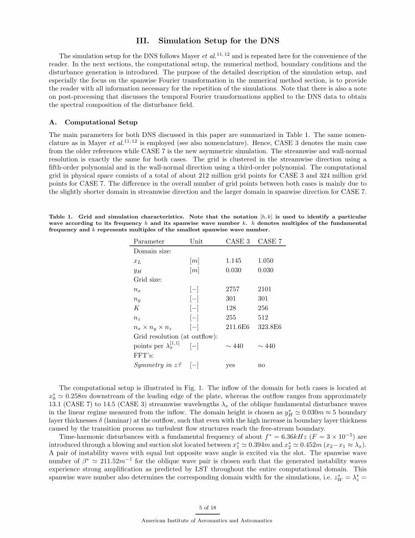
III. Simulation Setup for the DNS

The simulation setup for the DNS follows Mayer et al.11, 12 and is repeated here for the convenience of thereader. In the next sections, the computational setup, the numerical method, boundary conditions and thedisturbance generation is introduced. The purpose of the detailed description of the simulation setup, andespecially the focus on the spanwise Fourier transformation in the numerical method section, is to providethe reader with all information necessary for the repetition of the simulations. Note that there is also a noteon post-processing that discusses the temporal Fourier transformations applied to the DNS data to obtainthe spectral composition of the disturbance field.


The main parameters for both DNS discussed in this paper are summarized in Table 1. The same nomen-clature as in Mayer et al.11, 12 is employed (see also nomenclature). Hence, CASE 3 denotes the main casefrom the older references while CASE 7 is the new asymmetric simulation. The streamwise and wall-normalresolution is exactly the same for both cases. The grid is clustered in the streamwise direction using afifth-order polynomial and in the wall-normal direction using a third-order polynomial. The computationalgrid in physical space consists of a total of about 212 million grid points for CASE 3 and 324 million gridpoints for CASE 7. The difference in the overall number of grid points between both cases is mainly due tothe slightly shorter domain in streamwise direction and the larger domain in spanwise direction for CASE 7.

Table 1. Grid and simulation characteristics. Note that the notation [h, k] is used to identify a particularwave according to its frequency h and its spanwise wave number k. h denotes multiples of the fundamentalfrequency and k represents multiples of the smallest spanwise wave number.

Parameter Unit CASE 3 CASE 7

Domain size:

xL [m] 1.145 1.050

yH [m] 0.030 0.030

Grid size:

nx [−] 2757 2101

ny [−] 301 301

K [−] 128 256

nz [−] 255 512

nx × ny × nz [−] 211.6E6 323.8E6

Grid resolution (at outflow):

points per λ[1,1]x [−] ∼ 440 ∼ 440

FFT’s:

Symmetry in z? [−] yes no

The computational setup is illustrated in Fig. 1. The inflow of the domain for both cases is located atx∗

0 ≃ 0.258m downstream of the leading edge of the plate, whereas the outflow ranges from approximately13.1 (CASE 7) to 14.5 (CASE 3) streamwise wavelengths λx of the oblique fundamental disturbance wavesin the linear regime measured from the inflow. The domain height is chosen as y∗

H ≃ 0.030m ≈ 5 boundarylayer thicknesses δ (laminar) at the outflow, such that even with the high increase in boundary layer thicknesscaused by the transition process no turbulent flow structures reach the free-stream boundary.

Time-harmonic disturbances with a fundamental frequency of about f∗ = 6.36kHz (F = 3 × 10−5) areintroduced through a blowing and suction slot located between x∗

1 ≃ 0.394m and x∗

2 ≃ 0.452m (x2−x1 ≈ λx).A pair of instability waves with equal but opposite wave angle is excited via the slot. The spanwise wavenumber of β∗ ≃ 211.52m−1 for the oblique wave pair is chosen such that the generated instability wavesexperience strong amplification as predicted by LST throughout the entire computational domain. Thisspanwise wave number also determines the corresponding domain width for the simulations, i.e. z∗W = λ∗

z =

5 of 18


2π/β∗ ≃ 0.03m. For CASE 3, only half of this spanwise domain width is simulated because of symmetry,while, for CASE 7, the entire domain must be considered.

H

��

��

xy

buffe

r do

mai

n

x0 x1

y

2x xL

x3

Figure 1. Illustration of the computational domain for CASE 3 and CASE 7.

B. Numerical Method

The governing equations are integrated in time by employing a fourth-order Runge–Kutta scheme. The spa-tial derivatives are discretized using formally fourth-order split-finite differences in the streamwise and wall-normal directions. The spanwise direction is assumed to be periodic and, therefore, transformed into spectralspace using Fast Fourier Transforms (FFT). Moreover, the spanwise discretization is pseudo-spectral,22 i.e.all nonlinear terms in the governing equations are computed in physical space and then transformed backinto spectral space. Two options are available for the spanwise Fourier transformations: (i) All flow variables(i.e. streamwise velocity u, wall-normal velocity v, etc.) are assumed to be symmetric to the centerplane,except for the spanwise velocity w, which is antisymmetric. Symmetric quantities are then transformed intoFourier space using a Fourier cosine transformation and antisymmetric variables (w) are transformed bya Fourier sine transformation. Thus, only one-half spanwise wave length λz has to be computed for thisconfiguration. (ii) No symmetry is assumed and, therefore, all variables are transformed using a full Fouriertransformation. This option requires the computation of the entire spanwise wave length λz .

The Fourier transformations are based on the VFFTPK library, which can be downloaded from netlib(http://www.netlib.org/vfftpack/). According to this library and its implementation in the Navier–Stokescode, a Fourier cosine transformation into spectral space and its inverse transformation into physical spaceare given by


φck ∼

1

2(nz − 1)

[φc

0 + 2

nz−1∑

l=1

φcl cos

(πkl

nz − 1

)], (15a)


φcl ∼ φc

0 + 2

K−1∑

k=1

φckcos

(πkl

nz − 1

), (15b)

for k = 0, ..., K − 1 and l = 0, ...., nz − 1, respectively. φck represents the Fourier amplitude for mode k.

Moreover, nz indicates the number of grid points used for resolving the spanwise direction in physical spaceover the interval [0, (nz − 1)∆z] with

∆z =λz

2(nz − 1)(16)

and K represents the number of modes in Fourier space (for the simulations nz = 2K − 1).

The Fourier sine transformation to spectral space, with φsk as the Fourier amplitude, and its inverse into

6 of 18


physical space are


φsk ∼ −

1

(nz − 1)

nz−1∑

l=1

φsl sin

(πkl

nz − 1

), (17a)


φsl ∼ −2

K−1∑

k=1

φsksin

(πkl

nz − 1

), (17b)

for k = 0, ..., K − 1 and l = 0, ...., nz − 1, respectively.In contrast to a symmetric simulation where only one-half of the spanwise wave length has to be calcu-

lated, an asymmetric simulation requires the entire spanwise wave length as computational domain. Hence,for symmetric simulations nz represents the number of grid points in one-half wave length, whereas forasymmetric simulations, this number depicts the grid points in one full spanwise wave length. In this case,the grid spacing in the spanwise direction is therefore obtained from

∆z =λz

(nz − 1). (18)

The full Fourier transformations for an asymmetric simulation are


φ0 ∼1

2nz

nz−1∑

l=0

φl , (19a)

φck ∼

1

nz

nz−1∑

l=0

φl cos

(2πkl

nz

), (19b)

φsk ∼

1

nz

nz−1∑

l=0

φl sin

(2πkl

nz

), (19c)


φl ∼ φ0 +

K−1∑

k=1

[φc

kcos

(2πkl

nz

)+ φs

ksin

(2πkl

nz

)], (19d)

with k = 0, ..., K − 1 and l = 0, ...., nz − 1. As for the symmetric case, K denotes the number of Fouriermodes. The entire storage space scales by 2K − 1 since the cosine modes and the sine modes have to bestored separately. More details on the numerical method as well as validation cases for the Navier–Stokescode can be found in the theses of Harris,23 von Terzi,24 and Mayer.25

C. Boundary Conditions

At the inflow, the conservative quantities ρ, ρui, and Et, obtained from the similarity solution of a com-pressible flat-plate boundary layer, are specified. The outflow is treated with a buffer domain technique26

to avoid reflections of disturbance waves. The buffer domain starts at x3 and ends at xL with a length ofxL − x3 ∼ 0.5λx (Fig. 1). At the free-stream boundary, all total flow quantities are separated into base flowand disturbance quantities. For the base-flow quantities, a homogeneous von Neumann condition is appliedwhereas for the disturbance quantities an exponential decay condition is employed that was derived for com-pressible flow using linear stability considerations.27 Periodicity is assumed in the spanwise direction. Atthe wall, the no-slip and no-penetration conditions are used except for the disturbance slot (see below). Inaddition, for the base flow, the wall temperature is set to the adiabatic wall temperature of the correspondinglaminar flow, i.e. the initial condition, whereas temperature fluctuations are assumed to vanish.

D. Disturbance Generation

The flow is forced through the disturbance slot by prescribing a time-harmonic function for the fundamentalspanwise Fourier mode of the v-velocity. During the start-up of the simulation, the forcing amplitude A(β)

7 of 18


is ramped up in time over one disturbance period. The velocity distribution vp over the blowing and suctionslot has the shape of a dipole and it is represented by a fifth-order polynomial that is smooth everywhereincluding at the end points

v (xp, y = 0, β, t) = A (β) vp (xp) cos (−ωt + θp (β)) . (20)

xp is defined as

xp(x) =2x − (x2 + x1)

x2 − x1for − 1 ≤ xp ≤ 1 , (21)

and vp as

vp(xp) =

1.54 (1 + xp)3(3 (1 + xp)

2− 7 (1 + xp) + 4

), xp ≤ 0

−1.54 (1 − xp)3(3 (1 − xp)

2− 7 (1 − xp) + 4

), xp > 0 .

(22)

The amplitude A = 0.003 and, without any loss of generality, θp = 0 for the DNS described herein.

E. Post-processing

In order to obtain the spectral composition of the disturbance field from the DNS in a post-processing step,the physical time signal is Fourier transformed in time. The post-processing tool is based on the EAS3 tool kitfrom the Universitat Stuttgart (http://en.wikipedia.org/wiki/EAS3). In EAS3, the Fourier transformationsare given as follows


φ0 ∼1

nt

nt−1∑

n=0

φn , (23a)

φm ∼1

nt

nt−1∑

n=0

2φn exp

(−i2πmn

nt

), (23b)

for m = 1, ..., M − 1 and M = nt/2. Here, M contains the number of Fourier modes and nt the number of

sample points of the physical signal. The output data of the tool is the absolute value |φm| and the negative

phase − arg(φm) of the complex number φm. The back transformation is defined as


φn ∼ Re

[M−1∑

m=0

φm exp

(i2πmn

nt

)], (24a)

for n = 0, ..., nt − 1.

IV. Simulation Setup for the PSE Approach

In this section, the simulation setup of the PSE calculation is given. The computational domain differsfrom the DNS due to the different theoretical and numerical approaches. A short discussion on the numericalmethod, the boundary conditions and initial condition is also provided.


The Reynolds number range and the disturbance frequency of the PSE calculations and of the DNS (CASE 3)are depicted in the stability diagram of Fig. 2. Two main PSE calculations have been performed, whichvary in the starting position for the marching procedure. For one PSE calculation, from hereon abbreviatedas PSE 1, the starting position is located close to the first neutral branch at xPSE1

0 = 0.068m (Rx ≃ 385)whereas, for the second PSE calculation, PSE 2, the domain starts at xPSE2

0 = 0.6m (Rx ≃ 1144). Thereasoning behind these choices is explained in section V.2. The domain height is chosen as 200×L∗, with L∗

being the similarity boundary-layer length scale. The boundary layer is disturbed by prescribing non-paralleleigenfunctions obtained from a precursor non-parallel stability analysis (for a frequency of f∗ = 6.36kHz

8 of 18


Rx

F

0 500 1000 1500 20000.0E+00

5.0E-05

1.0E-04

1.5E-04

35

7

9

10

6

7

9

7

8

9

10

10

10

x0PSE2

xLDNSx0

DNS

x0PSE1

Rx

F

0 500 1000 1500 20000.0E+00

5.0E-05

1.0E-04

1.5E-04Level α i

10 09 -0.0002151928 -0.0004303847 -0.0006455776 -0.0008607695 -0.001075964 -0.001291153 -0.001506352 -0.001721541 -0.00193673

Figure 2. Stability diagram for β∗ ≃ 211.52m

−1 used to illustrate the computational domain for the PSEcalculations. The box between Rx = 927 and Rx = 993 indicates the position of the blowing and suction slot inthe DNS.

and a spanwise wave number of β∗ ≃ 211.52m−1) at the inflow. The spanwise direction is assumed to besymmetric and is discretized using Fourier transformations. The number of Fourier modes for the obliquebreakdown computations is selected to ensure an O(10−4) decay in amplitude from the most energetic modesto the tail of the disturbance spectrum. The wall-normal direction is resolved by 171 points with clusteringof grid points near the surface as well as the critical layer of the first-mode type waves.

B. Numerical Method

The governing linear and nonlinear PSEs are solved by a fourth-order central difference scheme in the wall-normal direction and by a first- or second-order one-sided difference scheme in the streamwise direction. Thespanwise direction is assumed to be periodic and therefore transformed into spectral space using Fouriertransforms. Furthermore, the spanwise discretization is pseudo-spectral,22 i.e. all nonlinear terms on theright-hand side of Eq. (12) are computed in physical space and then transformed back into spectral space. Asfor the DNS, the spanwise direction can be set to be symmetric in u-velocity, v-velocity, temperature, density,and pressure and antisymmetric in w-velocity reducing the computational domain to half a fundamentalspanwise wave length λ∗

z. This approach is adopted for the present paper. Details on the discretizationscheme can be found in Chang.28

C. Initialization of PSE Calculations and Boundary Conditions

To initialize the PSE analysis, mean-flow data for all streamwise positions and the disturbance informationat the starting location of the streamwise marching procedure are required. A convenient way to initializethe PSE analysis is to prescribe eigenfunctions from LST. This approach, however, would result in a “tran-sient” region where the PSE solution transitions from the LST eigenfunctions, satisfying parallel theory, atthe inflow to the solution of the non-parallel parabolized stability equations. Hence, in the present work,eigenfunctions obtained from a precursor non-parallel stability analysis are used. The mean-flow data stemsfrom a compressible similarity solution with adiabatic wall boundary condition. The differences between thesimilarity solution and the DNS mean flow were found to be negligible. At the wall, the no-slip conditionis enforced and temperature fluctuations are set to zero while at the free stream, non-reflective boundaryconditions are employed.

9 of 18


V. Results and Discussion

The results section is split into three main parts. The first part gives a summary of the main findingsfor CASE 3 in the transitional regime, which are similar to CASE 2 in Mayer et al.11 Note that CASE 3 issymmetric in spanwise direction since, so far in the literature, oblique breakdown has always been initiatedby two symmetric, oblique, first-mode type instability waves. Furthermore, the results of CASE 3 arecomplemented by discussing CASE 7, for which the symmetry restriction is removed. The second part ofthis section (section V.B) is focused on longer time averages for the turbulent regime and their comparisonwith shorter time averages from Mayer et al.12 The final part of the results section (section V.C) provides acomparison of PSE results obtained from NASA’s LASTRAC code to results from CASE 3 for the receptivityregime and the early nonlinear transition regime of oblique breakdown. This comparison provides additionalvalidation of the DNS setup and the nonlinear PSE approach of LASTRAC.

A. Removing the Symmetry Condition in the Spanwise Direction

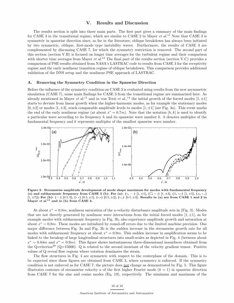
Before the influence of the symmetry condition on CASE 3 is evaluated using results from the new asymmetricsimulation (CASE 7), some main findings for CASE 3 from the transitional regime are summarized here. Asalready mentioned in Mayer et al.11 and in von Terzi et al.,14 the initial growth of the forced modes [1,±1]starts to deviate from linear growth when the higher-harmonic modes, as for example the stationary modes[0,±2] or modes [1,±3], reach comparable amplitude levels to modes [1,±1] (see Fig. 3a). This event marksthe end of the early nonlinear regime (at about x∗ = 0.7m). Note that the notation [h, k] is used to identifya particular wave according to its frequency h and its spanwise wave number k. h denotes multiples of thefundamental frequency and k represents multiples of the smallest spanwise wave number.

0.3 0.4 0.5 0.6 0.7 0.8 0.9 1.0x

*, m

1.0e-06

1.0e-04

1.0e-02

|u’| m

ax

0.3 0.4 0.5 0.6 0.7 0.8 0.9 1.0 1.1x

*, m

1.0e-04

1.0e-03

1.0e-02

1.0e-01

|u| [h

,k]m

ax

(a) (b)

Figure 3. Streamwise amplitude development of mode shape maximum for modes with fundamental frequency(a) and subharmonic frequency from CASE 3 (b): For (a): (◦, —) [1,±1], (�, - -) [1,±3], (♦, -.-) [1,±5], (△, -..)[1,±7]); For (b): (—) [0.5, 0], (- -) [0.5,±1], (-.-) [0.5,±2], (-..) [0.5,±3]. Results in (a) are from CASE 1 and 2 inMayer et al.11 and in (b) from CASE 3.

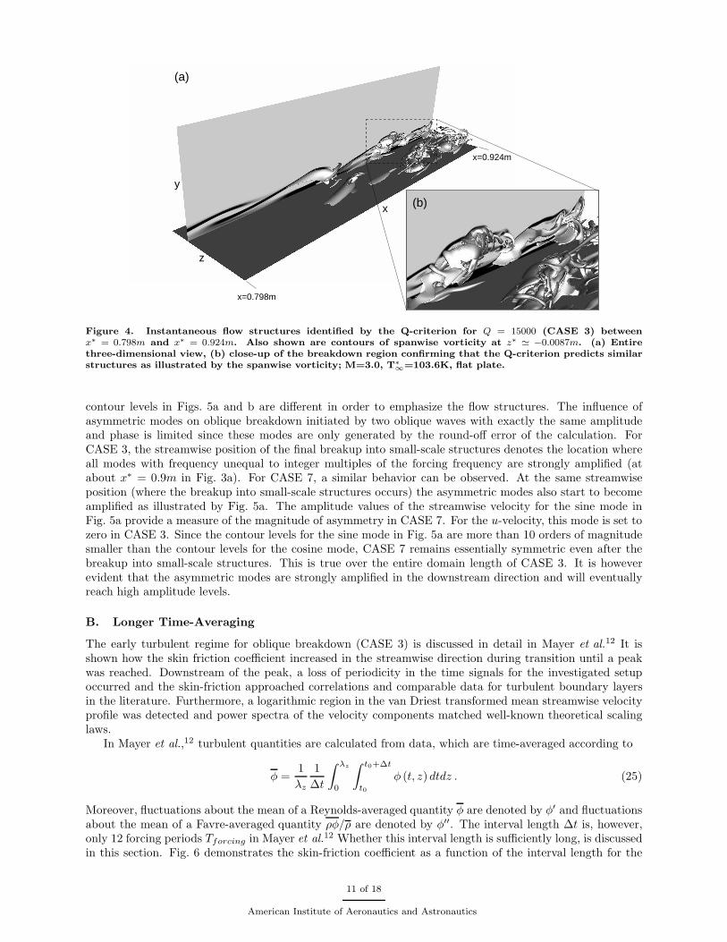
At about x∗ = 0.8m, nonlinear saturation of the u-velocity disturbance amplitude sets in (Fig. 3). Modesthat are not directly generated by nonlinear wave interactions from the initial forced modes [1,±1], as forexample modes with subharmonic frequency in Fig. 3b, also experience amplitude growth and saturation atabout x∗ = 0.8m. These modes are initialized by round-off errors due to the limited machine precision. Onemajor difference between Fig. 3a and Fig. 3b is the sudden increase in the streamwise growth rate for allmodes with subharmonic frequency at about x∗ = 0.9m. This sudden increase in amplification seems to belinked to the breakup of large longitudinal structures into small-scales as depicted in Fig. 4 (between aboutx∗ = 0.84m and x∗ = 0.9m). This figure shows instantaneous three-dimensional isosurfaces obtained fromthe Q-criterion29 (Q=15000). Q is related to the second invariant of the velocity gradient tensor. Positivevalues of Q reveal flow regions where rotation dominates the strain.

The flow structures in Fig. 4 are symmetric with respect to the centerplane of the domain. This is tobe expected since these figures are obtained from CASE 3, where symmetry is enforced. If the symmetrycondition is not enforced as for CASE 7, the picture does not change as demonstrated by Fig. 5. This figureillustrates contours of streamwise velocity u of the first higher Fourier mode (k = 1) in spanwise directionfrom CASE 7 for the sine and cosine modes (Eq. 19), respectively. The minimum and maximum of the

10 of 18


z

y

x

(a)

(b)

x=0.924m

x=0.798m

Figure 4. Instantaneous flow structures identified by the Q-criterion for Q = 15000 (CASE 3) betweenx∗ = 0.798m and x

∗ = 0.924m. Also shown are contours of spanwise vorticity at z∗ ≃ −0.0087m. (a) Entire

three-dimensional view, (b) close-up of the breakdown region confirming that the Q-criterion predicts similarstructures as illustrated by the spanwise vorticity; M=3.0, T∗

∞=103.6K, flat plate.

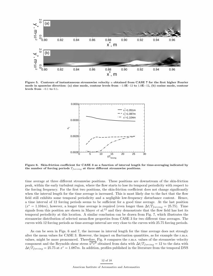
contour levels in Figs. 5a and b are different in order to emphasize the flow structures. The influence ofasymmetric modes on oblique breakdown initiated by two oblique waves with exactly the same amplitudeand phase is limited since these modes are only generated by the round-off error of the calculation. ForCASE 3, the streamwise position of the final breakup into small-scale structures denotes the location whereall modes with frequency unequal to integer multiples of the forcing frequency are strongly amplified (atabout x∗ = 0.9m in Fig. 3a). For CASE 7, a similar behavior can be observed. At the same streamwiseposition (where the breakup into small-scale structures occurs) the asymmetric modes also start to becomeamplified as illustrated by Fig. 5a. The amplitude values of the streamwise velocity for the sine mode inFig. 5a provide a measure of the magnitude of asymmetry in CASE 7. For the u-velocity, this mode is set tozero in CASE 3. Since the contour levels for the sine mode in Fig. 5a are more than 10 orders of magnitudesmaller than the contour levels for the cosine mode, CASE 7 remains essentially symmetric even after thebreakup into small-scale structures. This is true over the entire domain length of CASE 3. It is howeverevident that the asymmetric modes are strongly amplified in the downstream direction and will eventuallyreach high amplitude levels.

B. Longer Time-Averaging

The early turbulent regime for oblique breakdown (CASE 3) is discussed in detail in Mayer et al.12 It isshown how the skin friction coefficient increased in the streamwise direction during transition until a peakwas reached. Downstream of the peak, a loss of periodicity in the time signals for the investigated setupoccurred and the skin-friction approached correlations and comparable data for turbulent boundary layersin the literature. Furthermore, a logarithmic region in the van Driest transformed mean streamwise velocityprofile was detected and power spectra of the velocity components matched well-known theoretical scalinglaws.

In Mayer et al.,12 turbulent quantities are calculated from data, which are time-averaged according to

φ =1

λz

1

∆t

∫ λz

0

∫ t0+∆t

t0

φ (t, z)dtdz . (25)

Moreover, fluctuations about the mean of a Reynolds-averaged quantity φ are denoted by φ′ and fluctuationsabout the mean of a Favre-averaged quantity ρφ/ρ are denoted by φ′′. The interval length ∆t is, however,only 12 forcing periods Tforcing in Mayer et al.12 Whether this interval length is sufficiently long, is discussedin this section. Fig. 6 demonstrates the skin-friction coefficient as a function of the interval length for the

11 of 18


x*, m0.80 0.82 0.84 0.86 0.88 0.90 0.92 0.94 0.96

y*, m

0.02.0

*10-2

x*, m0.80 0.82 0.84 0.86 0.88 0.90 0.92 0.94 0.96

y*, m

0.02.0

*10-2

(a)

(b)

Figure 5. Contours of instantaneous streamwise velocity u obtained from CASE 7 for the first higher Fouriermode in spanwise direction: (a) sine mode, contour levels from −1.0E−12 to 1.0E−12, (b) cosine mode, contourlevels from −0.1 to 0.1.

0 5 10 15 20 25 30t/Tforcing

0.0028

0.0029

0.0030

0.0031

c f

x*=1.051m

x*=1.087m

x*=1.104m

Figure 6. Skin-friction coefficient for CASE 3 as a function of interval length for time-averaging indicated bythe number of forcing periods Tforcing at three different streamwise positions.

time average at three different streamwise positions. These positions are downstream of the skin-frictionpeak, within the early turbulent region, where the flow starts to lose its temporal periodicity with respect tothe forcing frequency. For the first two positions, the skin-friction coefficient does not change significantlywhen the interval length for the time average is increased. This is most likely due to the fact that the flowfield still exhibits some temporal periodicity and a negligible low-frequency disturbance content. Hence,a time interval of 12 forcing periods seems to be sufficient for a good time average. At the last position(x∗ = 1.104m), however, a longer time average is required (even longer than ∆t/Tforcing = 25.75). Timesignals from this position are shown in Mayer et al.12 and they demonstrate that the flow field has lost itstemporal periodicity at this location. A similar conclusion can be drawn from Fig. 7, which illustrates thestreamwise distribution of selected mean-flow properties from CASE 3 for two different time averages. Thecurves with 12 forcing periods as time-average interval are very close to the curves with 25.75 forcing periods.

As can be seen in Figs. 6 and 7, the increase in interval length for the time average does not stronglyalter the mean values for CASE 3. However, the impact on fluctuation quantities, as for example the r.m.s.values, might be more pronounced. Therefore, Fig. 8 compares the r.m.s. values of the streamwise velocitycomponent and the Reynolds shear stress u′′v′′ obtained from data with ∆t/Tforcing = 12 to the data with∆t/Tforcing = 25.75 at x∗ = 1.087m. In addition, profiles published in the literature from the temporal DNS

12 of 18


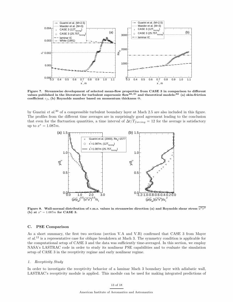
0.3 0.4 0.5 0.6 0.7 0.8 0.9 1.0 1.1x

*, m

0.000

0.001

0.002

0.003

0.004

c f



laminar ICWhite (1991)

(a)

0.3 0.4 0.5 0.6 0.7 0.8 0.9 1.0 1.1x

*, m

0

1000

2000

3000

Re Θ



laminar IC

(b)

Figure 7. Streamwise development of selected mean-flow properties from CASE 3 in comparison to differentvalues published in the literature for turbulent supersonic flow30,31 and theoretical models:32 (a) skin-frictioncoefficient cf , (b) Reynolds number based on momentum thickness Θ.

by Guarini et al.30 of a compressible turbulent boundary layer at Mach 2.5 are also included in this figure.The profiles from the different time averages are in surprisingly good agreement leading to the conclusionthat even for the fluctuation quantities, a time interval of ∆t/Tforcing = 12 for the average is satisfactoryup to x∗ = 1.087m.

0.0 1.0 2.0 3.0(ρ/ρw)

0.5(u"u")

0.5/uτ

0.0

0.5

1.0

1.5

y/δ c

Guarini et al. (2000), Reθ=1577

x*=1.087m, (12Tforcing)

x*=1.087m (25.75Tforcing)

-1.2-1.0-0.8-0.6-0.4-0.2 0.0(ρ/ρw)(u"v")/uτ

2

0.0

0.5

1.0

1.5y/

δ c(a) (b)

Figure 8. Wall-normal distribution of r.m.s. values in streamwise direction (a) and Reynolds shear stress u′′v′′

(b) at x∗ = 1.087m for CASE 3.

C. PSE Comparison

As a short summary, the first two sections (section V.A and V.B) confirmed that CASE 3 from Mayeret al.12 is a representative case for oblique breakdown at Mach 3. The symmetry condition is applicable forthe computational setup of CASE 3 and the data was sufficiently time-averaged. In this section, we employNASA’s LASTRAC code in order to study its nonlinear PSE capabilities and to evaluate the simulationsetup of CASE 3 in the receptivity regime and early nonlinear regime.

1. Receptivity Study

In order to investigate the receptivity behavior of a laminar Mach 3 boundary layer with adiabatic wall,LASTRAC’s receptivity module is applied. This module can be used for making integrated predictions of

13 of 18


receptivity and subsequent evolution of instability waves for certain simple classes of receptivity mechanisms,including the receptivity to unsteady blowing and suction at the surface (as in CASE 3). Before presentingany results for the instability wave perturbations excited by the unsteady blowing and suction slot fromEq. (20), we intend to explain the receptivity behavior of a supersonic boundary layer to this form of forcingin general. As described in the context of the DNS results, a localized blowing and suction slot excitesthe first mode-type instability wave at the frequency (and spanwise wave number) of excitation as well asother disturbances that are stable and, hence, do not influence the disturbance dynamics sufficiently fardownstream. We confine our attention to the instability wave portion of the boundary layer response andexamine how well the theoretical models (and, in particular, the model based on adjoint PSE20) can predictthe first-mode type perturbations in this specific case. The theoretical prediction for the instability waveperturbations due to the surface actuator can be expressed in the form of Eq. (11), where

ǫ =1

√2π

∫ x

x0

Λ (ξ, β) F (ξ, β) exp (−iθr (ξ, β)) dξ . (26)

Here, the efficiency function Λ represents the instability wave portion of the Green’s function associated withthe boundary layer response to this type of wall forcing, i.e., the effective initial amplitude of the instabilitywave due to a point source actuation. It characterizes the intrinsic receptivity characteristics of the localboundary layer to a specific type of forcing and is independent of the spatial distribution of the source. Thedependence on the source geometry is reflected via the convolution of the efficiency function Λ with thespanwise Fourier transfrom of the unsteady blowing and suction velocity vp from Eq. (20)

F (x, β) =1

2Avp (x) . (27)

The quantity θr in Eq. (26) denotes the phase of the velocity perturbation

θr (x, β) =

∫ x

x0

αr (ξ, β) dξ . (28)

1

1

Figure 9. Receptivity behavior of a laminar Mach 3 boundary layer with adiabatic wall due to blowing andsuction according to Eq. (20) applied in CASE 3: (a) efficiency function Λ from PSE as a function of streamwiseposition x, and (b) predicted amplitude value for modes [1,±1] from PSE (solid line) and from DNS (dot) atposition x

∗ = 0.5m as a function of starting position of disturbance slot x1. Note that the inset in (b) showsthe combined amplitudes of modes [±1,±1].

Fig. 9 illustrates the magnitude of the efficiency function Λ, plotted as a function of the streamwise sourcelocation x. The choice of normalization of the efficiency function is the same as in Chang and Choudhari.20

It can be seen in Fig. 9a that the intrinsic efficiency values vary weakly with the source location, with lessthan 33% variation over a broad range of actuator locations. Thus, the dominant effect of source locationon the amplitude of modes [1,±1] is due to the progressive reduction in the linear amplification potential

14 of 18


associated with source locations downstream of the first neutral branch. This effect is reflected in the strongreduction in the amplitude of modes [1,±1] at x∗ = 0.5m as the starting location for the blowing and suctionslot is varied along the streamwise direction in Fig. 9b. Note that, for the results plotted in this figure, themeasurement location is sufficiently downstream of the source, but still within a predominantly linear regionin terms of the fundamental mode evolution. The amplitude of the instability wave extracted from theDNS computation (shown as a dot in Fig. 9b) is within 3% of the value predicted by the theory. Thissmall discrepancy could be even further narrowed by accounting for the cumulative effects of disturbancenonlinearity between the disturbance slot and the measurement location, but was deemed unnecessary.

2. Finite Amplitude Forcing

The early nonlinear regime of oblique breakdown at Mach 3 is studied by performing PSE calculations withtwo different simulation setups. As already mentioned in section IV.A, the first setup starts at the firstneutral branch (PSE 1) while the second PSE calculation starts at x∗ = 0.6m (PSE 2). For PSE 1, theinitial disturbance amplitudes of modes [1,±1] at the neutral branch are scaled in order to match the absoluteamplitude values from the DNS farther downstream for this mode, while for PSE2, the initial amplitudes ofthe first 6 dominant modes ([1,±1], [0,±2], and [1,±3]) are scaled to the corresponding values from the DNSat x∗ = 0.6m. The reasoning for the setup PSE 1 is to examine whether the DNS results (CASE 3) can be

(a) (b)

(c)

Figure 10. Streamwise amplitude development of the wall-normal maximum (mode shape maximum) forselected modes calculated from physical data according to the Fourier transforms given in Eqs. (15) and (23):(a) (symbols) PSE 1, (dashed lines) DNS, (b) (symbols) PSE 2, (dashed lines) DNS. (c) Setup from PSE 1,but with (solid lines) and without (symbols) the suppression of modes [0,±2].

15 of 18


completely recovered by a PSE calculation starting with a very low disturbance amplitude at the first neutralbranch, which would be the case during natural transition (i.e. without an artificial disturbance source atthe plate surface as employed in the DNS). As shown in Fig. 10a, which illustrates the streamwise amplitudedevelopment of the wall-normal maximum (mode shape maximum) for selected modes, the DNS cannot becompletely recovered resulting in a discrepancy between the nonlinear generated modes from the DNS andthe nonlinear PSE analysis. This difference is mainly caused by nonlinear effects during the receptivityprocess in the DNS since the forcing amplitude of the DNS is already quite large (A=0.3%). If in a secondPSE analysis the setup is changed to PSE 2 so that the amplitudes of not just the fundamental, but alsothe most dominant nonlinearly excited modes are matched with the DNS, then the agreement between thedata from PSE and the data from DNS improves significantly as demonstrated in Fig. 10b.

We also examined the effect of suppressing modes [0,±2] to disrupt the energy cascade from modes[1,±1] to their higher-harmonic modes associated with oblique breakdown. Mode [0,±2] was canceled outby a modest stationary forcing at x∗ = 0.6m in a new PSE calculation for setup PSE 1. Fig. 10c showsthe results corresponding to this simulation. Symbols refer to the PSE results from Fig. 10a, where modes[0,±2] are not suppressed and solid lines represent the new simulation. Clearly, the influence of nonlinearwave interactions is weakend resulting in a delay of transition. While the delay in transition onset locationis approximately 5% increased, it may be less in a natural disturbance environment.

(a) (b)

Figure 11. Streamwise development of skin friction coefficient: (a) (solid line) DNS, (symbols) PSE, (b) PSEwith (solid line) and without (dashed line) suppression of modes [0,±2].

The previously mentioned findings are confirmed by the streamwise development of the skin frictioncoefficient in Fig. 11. The comparison between DNS and PSE results (PSE 2) in Fig. 11a leads to anexcellent agreement between both methods indicating that nonlinear PSE is able to predict the transitiononset correctly. In fact, the agreement extends up to the location, where the skin friction coefficient is nearlytwice the value of the underlying laminar skin friction. This suggests that (i) the PSE results could, perhaps,be bridged with a turbulence model to provide integrated predictions of transition and turbulence33 and thatsuch PSE results could be used, as a cost effective means, to initiate simulations of fully turbulent boundarylayers. For the case with suppressed modes [0,±2], the transition onset is indeed moved downstream asdepicted in Fig. 11b.

VI. Conclusions

Transition to turbulence via oblique breakdown in a Mach 3 boundary layer was investigated usingDNS and PSE. Our previous studies of the same case focused on the detailed documentation of the differenttransition stages and demonstrated that oblique breakdown can lead to a fully developed turbulent boundarylayer. In these studies, however, the flow was assumed to be symmetric in the spanwise direction. Anew DNS was performed where the symmetry condition was removed. This simulation demonstrated thatoblique breakdown, initialized by two oblique instability waves with exactly the same amplitude level, losesits symmetry late in the turbulent stage for a low-noise environment. Hence, for the streamwise extent of

16 of 18


the computational domain in this study, the symmetry condition is justified. Furthermore, new data froma longer time average of the original symmetric simulation of oblique breakdown (CASE 3) was discussed.These data confirm that a converged time average is reached. The final part of the paper focused on acomparison of PSE results obtained from NASA’s LASTRAC code to the DNS results all the way fromthe disturbance generation to the initial part of the breakdown process. Good agreement was found for alldifferent transition stages, including receptivity, linear, and nonlinear disturbance evolution, and the initialpart of the breakdown process until the mean wall shear had nearly doubled with respect to its laminarvalue. Thus, the present paper corroborates that our oblique breakdown case for Mach 3 constitutes ageneric reference case that can be successfully used to validate different engineering tools, as for examplethe PSE approach, across the different transition stages. Furthermore, the PSE approach combined withturbulence models for transitional flow might be a sophisticated solution for modeling the entire transitionprocess of a supersonic boundary layer.

Acknowledgments

This work was partially funded by the Air Force Office for Scientific Research under grant FA9550-08-1-0211 with Dr. John Schmisseur serving as program manager. The computer hours and the technical supportprovided by NASA Ames are greatly acknowledged.

References

1Berry, S. A., Hamilton, H. H., and Wurster, K. E., “Effect of Computational Method on Discrete Roughness Correlations

for Shuttle Orbiter,” Journal of Spacecraft and Rockets, Vol. 43, No. 4, 2006, pp. 842–852.2Reshotko, E., “Is Reθ/Me a Meaningful Transition Criterion?” AIAA-2007-0943, 2007.3Mack, L. M., “Boundary-Layer Stability Theory,” Internal Document 900-277, Jet Propulsion Laboratory, Pasadena,

California, 1969.4Fedorov, A. V., “Receptivity of a high-speed boundary layer to acoustic disturbances,” J. Fluid Mech., Vol. 491, 2003,

pp. 101–129.5Tumin, A., “Three-Dimensional Spatial Normal Modes in Compressible Boundary Layers,” J. Fluid Mech., Vol. 586,

2007, pp. 295–322.6Fasel, H., Thumm, A., and Bestek, H., “Direct Numerical Simulation of Transition in Supersonic Boundary Layer:

Oblique Breakdown,” Transitional and Turbulent Compressible Flows, edited by L. D. Kral and T. A. Zang, No. 151 in FED,

ASME, 1993, pp. 77–92.7Kosinov, A. D., Semionov, N. V., Shevelkov, S. G., and Zinin, O. I., “Experiments on the Nonlinear Instability of

Supersonic Boundary Layers,” Nonlinear Instability of Nonparallel Flows, edited by D. T. Valentine, S. P. Lin, and W. R. C.

Philips, Springer, 1994, pp. 196–205.8Corke, T. C., Cavalieri, D. A., and Matlis, E., “Boundary-Layer Instability on Sharp Cone at Mach 3.5 with Controlled

Input,” AIAA J., Vol. 40, No. 5, 2002, pp. 1015–1018.9Mayer, C. S. J., Wernz, S., and Fasel, H. F., “Investigation of Oblique Breakdown in a Supersonic Boundary Layer at

Mach 2 Using DNS,” AIAA-2007-0949, 2007.10Mayer, C. S. J. and Fasel, H. F., “Investigation of Asymmetric Subharmonic Resonance in a Supersonic Boundary Layer

at Mach 2 Using DNS,” AIAA-2008-0591, 2008.11Mayer, C. S. J., von Terzi, D. A., and Fasel, H. F., “DNS of Complete Transition to Turbulence Via Oblique Breakdown

at Mach 3,” AIAA-2008-4398, 2008.12Mayer, C. S. J., von Terzi, D. A., and Fasel, H. F., “DNS of Complete Transition to Turbulence Via Oblique Breakdown

at Mach 3: Part. II,” AIAA-2009-3558, 2009.13Mayer, C. S. J., Laible, A. C., and Fasel, H. F., “Numerical Investigation of Transition initiated by a Wave Packet on a

Cone at Mach 3.5,” AIAA-2009-3809, 2009.14von Terzi, D. A., Mayer, C. S. J., and Fasel, H. F., “The Late Nonlinear Stage of Oblique Breakdown to Turbulence

in a Supersonic Boundary Layer,” Seventh Symposium on Laminar-Turbulent Transition, edited by P. Schlatter and D. S.

Henningson, Springer, 2009, pp. 415–420.15Kosinov, A. D., Semionov, N. V., and Shevelkov, S. G., “Investigation of Supersonic Boundary Layer Stability and

Transition Using Controlled Disturbances,” Methods of Aerophysical Research, edited by A. M. Kharitonov, Vol. 2, 1994, pp.

159–166.16Ermolaev, Y. G., Kosinov, A. D., and Semionov, N. V., “Experimental Investigation of Laminar-Turbulent Transition Pro-

cess in Supersonic Boundary Layer Using Controlled Disturbances,” Nonlinear Instability and Transition in Three-Dimensional

Boundary Layers, edited by P. W. Duck and P. Hall, Kluwer Academic Publishers, 1996, pp. 17–26.17Kosinov, A. D., Maslov, A. A., and Semionov, N. V., “An Experimental Study of Generation of Unstable Disturbances

on the Leading Edge of a Plate at M=2,” J. Appl. Mech. Tech. Phys., Vol. 38, No. 1, 1997, pp. 45–50.18Jiang, L., Choudhari, M., Chang, C.-L., and Liu, C., “Numerical Simulations of Laminar-Turbulent Transition in Super-

sonic Boundary Layer,” AIAA-2006-3224, 2006.

17 of 18


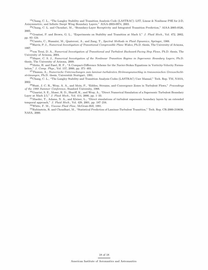
19Chang, C. L., “The Langley Stability and Transition Analysis Code (LASTRAC): LST, Linear & Nonlinear PSE for 2-D,

Axisymmetric, and Infinite Swept Wing Boundary Layers,” AIAA-2003-0974, 2003.20Chang, C. L. and Choudari, M., “Boundary-Layer Receptivity and Integrated Transition Prediction,” AIAA-2005-0526,

2005.21Graziosi, P. and Brown, G. L., “Experiments on Stability and Transition at Mach 3,” J. Fluid Mech., Vol. 472, 2002,

pp. 83–124.22Canuto, C., Hussaini, M., Quateroni, A., and Zang, T., Spectral Methods in Fluid Dynamics, Springer, 1988.23Harris, P. J., Numerical Investigation of Transitional Compressible Plane Wakes, Ph.D. thesis, The University of Arizona,

1997.24von Terzi, D. A., Numerical Investigation of Transitional and Turbulent Backward-Facing Step Flows, Ph.D. thesis, The

University of Arizona, 2004.25Mayer, C. S. J., Numerical Investigation of the Nonlinear Transition Regime in Supersonic Boundary Layers, Ph.D.

thesis, The University of Arizona, 2009.26Meitz, H. and Fasel, H. F., “A Compact-Difference Scheme for the Navier-Stokes Equations in Vorticity-Velocity Formu-

lation,” J. Comp. Phys., Vol. 157, 2000, pp. 371–403.27Thumm, A., Numerische Untersuchungen zum laminar-turbulenten Stromungsumschlag in transsonischen Grenzschicht-

stromungen, Ph.D. thesis, Universitat Stuttgart, 1991.28Chang, C. L., “The Langley Stability and Transition Analysis Codes (LASTRAC) User Manual,” Tech. Rep. TM, NASA,

2002.29Hunt, J. C. R., Wray, A. A., and Moin, P., “Eddies, Streams, and Convergence Zones in Turbulent Flows,” Proceedings

of the 1988 Summer Conference, Stanford University, 1988.30Guarini, S. E., Moser, R. D., Shariff, K., and Wray, A., “Direct Numerical Simulation of a Supersonic Turbulent Boundary

Layer at Mach 2.5,” J. Fluid Mech., Vol. 414, 2000, pp. 1–33.31Maeder, T., Adams, N. A., and Kleiser, L., “Direct simulations of turbulent supersonic boundary layers by an extended

temporal approach,” J. Fluid Mech., Vol. 429, 2001, pp. 187–216.32White, F. M., Viscous Fluid Flow , McGraw-Hill, 1991.33Rubinstein, R. and Choudhari, M., “Statistical Prediction of Laminar-Turbulent Transition,” Tech. Rep. CR-2000-210638,

NASA, 2000.

18 of 18


detailed comparison of dns to pse for oblique … comparison of dns to pse for ... nism if it can...

Documents