DESIGN OF HEADWORK FOR LOWER NAGAVALI

IRRIGATION PROJECT

A THESIS SUBMITTED IN PARTIAL FULFILLMENT OF

THE REQUIREMENTS FOR THE DEGREE OF

Bachelor of Technology

In

Civil Engineering

BY

BALKRISHNA PANGENI

ROLL NO: 109CE0055

DEPARTMENT OF CIVIL ENGINEERING

NATIONAL INSTITUTE OF TECHNOLOGY

ROURKELA 769008

MAY 2013

ii

DESIGN OF HEADWORK FOR LOWER NAGAVALI

IRRIGATION PROJECT

A THESIS SUBMITTED IN PARTIAL FULFILLMENT OF

THE REQUIREMENTS FOR THE DEGREE OF

Bachelor of Technology

In

Civil Engineering

BY

BALKRISHNA PANGENI

ROLL NO: 109CE0055

Under the guidance of

Prof. K.C Patra Department of Civil Engineering

National Institute of Technology, Rourkela

DEPARTMENT OF CIVIL ENGINEERING

NATIONAL INSTITUTE OF TECHNOLOGY

ROURKELA 769008

MAY 2013

iii

DEPARTMENT OF CIVIL ENGINEERING

NATIONAL INSTITUTE OF TECHNOLOGY

ROURKELA 769008

CERTIFICATE

This is to certify that the thesis entitled “Design of Headwork for Lower Nagavali

Irrigation Project” submitted by Balkrishna Pangeni (Roll Number: 109CE0055) in

partial fulfillment of the requirements for the award of Bachelor of Technology in the

Department of Civil Engineering, National Institute of Technology, Rourkela is an

authentic work carried out under my supervision and guidance.

To the best of my knowledge, the matter embodied in the thesis has not been submitted to

elsewhere for the award of any degree.

Place: Rourkela Prof. K.C Patra

Date: Civil Engineering Department

National Institute of Technology, Rourkela

iv

DEPARTMENT OF CIVIL ENGINEERING

NATIONAL INSTITUTE OF TECHNOLOGY

ROURKELA 769008

A C K N O W L E D G E M E N T

It gives me immense pleasure to express my deep sense of gratitude to my supervisor Prof.

K.C. Patra for his invaluable guidance, motivation, constant inspiration and above all for

his ever co-operating attitude that enabled me in bringing up this thesis in the present form.

I am extremely thankful to Prof. N. Roy, Head of Department, and Department of Civil

Engineering Department for providing all kinds of possible help and advice during the

course of this work.

I am greatly thankful to Prof. S.K. Das, all the staff members of the department and my

entire well-wishers, class mates and friends for their inspiration and help.

Place: Rourkela Balkrishna Pangeni

Date: B. Tech. (Roll: 109CE0055)

Civil Engineering Department

National Institute of Technology, Rourkela

v

ABSTRACT

This paper discuss about the design methodology of a dam and its stability against failure for a

Irrigation project. Most of the people of Rayagada district has taken agriculture as their means of

living and they are mostly dependent on seasonal rainfall for cultivation. This dependeny on direct

rainfall water for the cultivation of crop has lead to the reduction in crop yield due to lack of

rainfall.So, in this paper, I have studied the hydrological feature of the area,analysed it and a

suitable section is designed considering the design flood and the discharge that can be made

avaialabe at the downstream.The dam is then analysed using a software, PLAXIS for its stability

and suitability.Finally, a complete profile of a ogee crested spillway is drawn.Successfull

implementation of this project will facilate irrigation water for Gross Command Area(GCA) of

14,000Ha and Cultivable Command Area(CCA) of 8,500 Ha.

vi

LIST OF TABLES

Table 4.1 Material property used.

Table 5.1 Rainfall data of Kalyanisinghpur(in mm)

Table 5.2: Rainfall data of Kashipur(in mm).

Table 5.3 Final Rainfall data of Kashipur including estimated rainfall.

Table 5.4 Mean Monthly Rainfall (in mm)

Table 5.5 Flood discharge.

Table. 5.6 Various coordinates of downstream profile.

Table. 5.7 Various coordinates of downstream profile.

vii

LIST OF FIGURES

Figure 3.1 Location of Project site.

Figure 4.1 Weightage area using Thiessen Polygon.

Figure 4.2 Cross-section of the dam.

Figure 4.3 Mess generation.

Figure 4.4 Phreatic line.

Figure 4.5 Different calculation stage.

Figure 5.1 Rainfall-Rainfall corelation for June(in mm).

Figure 5.2 Rainfall-Rainfall corelation for July (in mm).

Figure 5.3 Rainfall-Rainfall corelation for August (in mm).

Figure 5.4 Rainfall-Rainfall corelation for September (in mm).

Figure 5.5 Rainfall-Rainfall corelation for October (in mm).

Figure 5.6 Syntheti Unit Hydrograph.

Figure 5.7 Design of cross section of dam.

Figure 5.8 Design of cross section of Rock toe and toe drain.

Figure 5.9 Safety factor of the design.

Figure 5.10 Active pore pressure.

Figure 5.11.Horizontal Total Stress.

Figure 5.12 Horizontal effective stress.

Figure 5.13 Vertical Strain.

Figure 5.14 Profile of Ogee Spillway

1

CHAPTER 1

INTRODUCTION

1.1 GENERAL OVERVIEW

In general,irrigation is the application of water to the soil for the purpose of supporting plant

growth.[1] Dependeny on direct rainfall water for the growth of crop may lead to reduction in

crop yield due to lack of rainfall. India with many large and small rivers, still faces the problem of

shortage of irrigation water due to the reason that people have to depend upon the seasonal rainfall

depending on the geographical location of the area. And the same river some time brings down

very high flood discharge leading to drowing down large area.Thus, requirement of irrigation water

is one problem and at the same time ,desingnig of dam and the canals for irrigation water supply.

The belief that large dams, by increasing irrigation and hydroelectricity production, can cause

development and reduce poverty has led developing countries and international agencies such as

the World Bank to undertake major investments in dam construction. By the year 2000, dams

generated 19 percent of the world's electricity supply and irrigated more than 30 percent of the

271 million hectares irrigated worldwide. However, these dams also displaced over 40 million

people, altered cropping patterns, and significantly increased salination and waterlogging of arable

land. India, which, with over 4,000 large dams, is the world's third most prolific dam builder (after

China and the United States) [2]. This is a very big number when compared to that of the word.But

still due to lack of technology and proper hydrology study and prior stability analysis, some dams

are found to be unsafe and many of them have failed.I have studied some of the dam that failed

2

and have analysed the reason for their failere which led me to design a safe dam for people of

Rayagada district who were in a real need of irrigation water for their living as most of the people

of that area are mainly dependend in agriculture for their living and source of economy.

Kaddam Project Dam, Andhra Pradesh, India, built in Adilabad ,in 1957 - 58, the dam was a

composite structure, earth fill and gravity dam. It was 30.78 m high and 3.28 m wide at its crest.

Its maximum full storage was was 1.366 * 108 𝑚3. The observed floods were 1.47 * 104 m3/s.

The dam was found to be overtopped by 46 cm of water above the crest, inspite of a free board

allowance of 2.4 m, causing a breach of 137.2 m wide that occurred on the left bank and led the

dam to fail in August 1985 right after one year of its construction.

The Kaila Dam in Kachch, Gujarat, India was constructed in between 1952 - 55 as an earthfill dam

with a height of 23.08 m above the river bed and 213.36 m crest length. Its full reservoir level was

13.98 million 𝑚3. The spillway was of ogee shaped and ungated. The depth of cutoff was 3.21 m

below the river bed. Inspite of a freeboard allowance of 3.96 m at the maximum reservoir level

the energy dissipation devices first failed and later the embankment collapsed due to the weak

foundation bed in 1959.

Similarly other dams like Kodaganar Dam constructed in Tamil Nadu, Machhu II (Irrigation

Scheme) Dam of Gujarat, Nanaksagar Dam of Punjab, Khadakwasla Dam of Maharashtra, India,

1864 - 1961) were found to be failed.[3] And the main reason behind their failure was found to be

lack of proper hydrology analysis that resulted in excess discharge in the dam than the it was

designed for and also due to improper or faulty desing and insufficient spillway.Considering these

historical fact of dam failure I have given utmost important to the hydrological analysis and then

stability check using reliable software, PLAXIS.I had collected the precipitation data from two

stations in the area namely Kalyanisinghpur and Kashipur that affects the flood discharge in the

river Nagavali.The precipitation data obtained from Kashipur station was from the year 1990-91

3

to 2009-10 and that of Kalyanisinghpur was from the year 1969-70 to 2009-10. The unknown

rainfall were then obtained by rainfall-rainfall correlation of these stations by using suitable

regression formula.

Following Hydrological and dam features were used during designing:

1.2 HYDROLOGY:

Hydrology is the study of origin, distribution and circulation of water in different forms in land

and atmosphere.In my project, I was basically concerned with collection of data and determination

of discharge with variation of time using hydrograph, being specific using Synders Synthetic Unit

Hydrograph.

1.2.1 Hydrograph

A hydrograph is a graph showing the rate of flow i.e. discharge with time in a river, or other

channel or conduit carrying flow.It is the total response or the output of a watershed beginning

with precipitation as the hydrological exciting agent or input.A hydrograph is a result three phases

namely base flow, subsurfaceand surface flow The rate of flow is usually expressed in cubic meters

or cubic feet per second.

1.2.2 Unit Hydrograph

An Unit Hydrograph (UH) or unit graph of a watershed is defined as the hydrograph of direct

runoff hydrograph resulting from a unit depth of 1 cm of excess rainfall of constant intensity

generated uniformly over the basin or drainage area occurring for a specified duration of D

hour.The term unit depth of rainfall excess means excess rainfall above and over all the losses (like

evaporation, transpiration,interception,depression storage and depression storage) in the basin for

which hydrograph is to be obtained.[4]

4

1.2.3 Snyder's Synthetic Unit Hydrograph

When a catchment is ungauged, the established empiracle formula or relation between the

catchment characteristics and unit hydrograph parameters may be used to synthesize a unit

hydrograph for a basin. A synthetic unit hydrograph has all the features of the unit hydrograph,

but it does not require rainfall-runoff data. A synthetic unit hydrograph is derived from the theory

and experience, and its purpose is to simulate basin diffusion by estimating the basin lag or lag

time based on a certain formula or procedure. The first synthetic unit hydrograph model was

developed by Snyder in 1938 [5] and is accepted as a standard practice for the derivation of a unit

hydrograph for a basin where rainfall and runoff datas are not available.

1.3 EARTHEN DAM

Any hydraulic structure that supplies water to the off-taking cannel is called a

headwork.Headworks my be divided into follwing two types :

1. Storage headwork.

2. Diversion headwork.

A diversion headwork is a hydraulic structure constructed to divert the required supply into the

canal from the river.

A storage headwork comprises the construction of a dam across a river valley so that water can be

stored during the period of excess water level in the river and release it when demand increases

above the available supplies.According to the most common type of classification a dam can be

classified into two types namely

1.Rigid Dams.

2.Non-Rigid Dams.

5

Rigid dams are those which are constructed using rigid materials like masonary,concrete,steel or

timber.They are further classified as follows:

1. Solid masonary or concrete gravity dam.

2. Arched masonary or concrete dam.

3. Concrete butress dam.

4. Steel dam.

5. Timber dam.

Non-rigid dams are those which are constructed using non-rigid materials like earth and/or rockfill

available near or away the site.They can be of following types:

a) 1.Earth dam.

b) 2.Rockfill dam.

c) 3.Combined earth and rockfill dam.

Earthen dams are the type of dam which are constructed using earth material available

economically or locally.These are the cheapest type of dam as they utilizes the locally available

materials, less skilled labour and primitive equipment.It is further divided into following three

types:

i. Homogeneous Embankment type

ii. Zoned Embankment type

iii. Diaphragm type.

We had opted for Homogeneous Embankment or Homogeneous earth dam during the construction

of which soil material is placed in thin layers(15 cm to 30 cm) and then compacted by using

rollers.It is the simplest type of an earthen dam which consists of single material and is

homogeneous throughout so it is called homogeneous type. A purely homogeneous type of dam is

6

composed of a single kind of material. Such purely homogeneous section, has now been replaced

by a modified homogeneous section in which considerable amount of pervious material is used to

control the action of seepage so as to allow much steeper slopes as compared to pure homogenous

dam. This type of dam is used when only one type of material is economically or locally available

around the site of construction. It is also used as it is economic due to requirement of less skilled

labour and primitive type of equipment during the construction.However larger dams are rarely

designed as homogeneous type because of the dam being more prone to failure due to seepage

and unstability. To overcome this problem, internal drainage system in the form of horizontal

blanket,rock toe and/or sand chimney is constructed inside the dam.

The main components of Homogeneous Earthen dams,their brief function and basic design

requrements are mentioned below;

Impervious Cut off: The cut off is located such that its centre line is within the base of

impervious core and is the upstream of centre line of dam.When the depth of the pervious

foundation strata is very large, a cutoff may be provided upto lesser depth.It is requred to

reduce the loss of stored water through foundations and to prevent sub-surface erosion by

piping of the foundation.

Internal drainage system and foundations: The water seeping through the body of earthen

dam and/or through the foundation is very harmfull as it weakens the stability of the dam

causing the softening of slopes due to the development of pore water pressure.Inorder to

control this seepage to a large extent,Internal drainge filters plays very important role.Such

drainage filters are generally provided in the form (i) rock toe (ii) horizontal blanket and

(ii) vertical or slanted sand chimney.

Drainage filter is one of the important part in the dam construction and it should be such

designe that neither embankment nor the foundation material can penetrate and clog the

7

filter.Terzaghi has given a rational approach to design the drainage filters which is given

as,

𝐷15 𝑜𝑓 𝑓𝑖𝑙𝑡𝑒𝑟

𝐷85 𝑜𝑓 𝑏𝑎𝑠𝑒 𝑚𝑎𝑡𝑒𝑟𝑖𝑎𝑙< 4 𝑡𝑜 5 <

𝐷15 𝑜𝑓 𝑓𝑖𝑙𝑡𝑒𝑟

𝐷15 𝑜𝑓 𝑏𝑎𝑠𝑒 𝑚𝑎𝑡𝑒𝑟𝑖𝑎𝑙

Base material here denotes the embankment soil or the foundation soil surrounding the

filter.

Slope protection: Due to the precipitation and water level in the reserviour,scouring of the

external slope surface can take place.In order to ensure this slope protection riprap is placed

at the outer slope in the upstream. A minimum of 300 mm thick riprap over 150 mm thick

filter layer may be generally provided upto the top of dam. In case of the downstream,slope

protection is ensured by turfing or riprap turfing on the entire downstream slope from top

of the dam to the toe.In addition, horizontal berms at suitable interval may be provided in

case of large dam to protect from the erosion action of rain and its run-off. The details on

downstream and upstream slope protection is clearly mentioned in IS 8237-1985.

1.4 STABILITY OF THE EARTHEN SLOPES

This is the most important part of this project. Designing a dam is not only of the prior

importance,designing it safe against failure criterion is the main deal. The constructed dam should

be safe against adverse materological condition and the geological feature of the location and the

dam itself. The following stability condition were taken into consideration for analysis as

mentioned below:

8

1. Stability of the downstream slope during steady seepage

2. Stability of the downstream slope under steady seepage from the consideration of

horizontal shear at base under downstream slope of the dam.

3. Stability of the foundation against shear.

4. Overall stability of the dam section.

All these stability check were done by using most popular and reliable Analysis software,

PLAXIS.

1.4.1 PLAXIS

PLAXIS is a finite element program designed for geotechnical applications in which soil models

are used to simulate the soil behaviour. In PLAXIS, stresses and strains are calculated at individual

Gaussian integration points rather than at individual nodes. The calculation stage requreis selection

of analysis type such as Plastic, dynamic, consolidation and phi-c reduction. The loads assigned

are activated here and analysed. In the post processing stage, plotting of curves between various

calculated parameters such as load vs displacement is done. Input parameters like stiffness and

poisson’s ratio of the soil influence the displacement of the slope. For stability check material

properties were first defined which we had obtained from the site of construction of the dam and

suitable soil material that were proposed to be used for the construction. The cross section of the

dam was drawn by using coordinate, after which material properties were assigned to the dam

section and the software was run to analyse the design and finally output was obtained based on

the type of construction used and the phreatic line given.

9

1.5 SPILLWAY:

Spillway is a passage constructed over or around a dam for the effective disposal of surplus water

from upstream to downstream when the reservoir itself is full. Spillways are particularly important

safety features for earth dam, protecting the dam and its foundation from erosion. They may lead

over the dam or a portion of it or along a channel around the dam or a conduit through it.[6] There

are six major types of spillway out of which we have chosen ogee crested spillway as it is improved

form of free overfall or straight drop spillway and is widely used with concrete,masonary, arch

and butress dams.

******

10

CHAPTER 2

LITERATURE SURVEY

Xu ,Y.Q.; Unami, K. and Kawachi, T. in their paper “Optimal hydraulic design of earth

dam cross section using saturated–unsaturated seepage flow model” formulated an optical

hydraulic design problem regarding an earth dam cross section for the steady model of saturated-

unsaturated seppage flows in porous media.The results showed that an inclined clay core of less

hydraulic conductivity should be located on the upstream side of the cross section and unsaturated

zone plays an inportant role in the flow field and the optimal design.

Tien-kuen,Hnang, in his paper “Stability analysis of an earth dam under steady state seepage” has

described the numerical procedure for performing stability analysis of an earth dam after the filling

of reserviour by using the piezometric heads at different points in an earth dam after filling the

reserviour.The result was analysed and sufficient factor of safety was found against the failure of

the dam. He concluded that sufficient factor of safety has to be ensured to prevent earth dam

against the failure.

Abolfazl Nazari Giglou, Taher Nazari Giglou and Afshar Minaei in their paper “Seepage through

Earth Dam” numerically analysed different homogeneous earth dams of height 5, 10, 20, 30, 40

and 50 m with a two-dimensional finite element code and they concluded that the seepage flow

rate depends on earth dam permeability coefficient (K), downstream and upstream slopes and the

total head (H) parameters.They also found that the rate of seepage discharge increase through the

earth dam with the increase of downstream slope amplitude angle.

11

Rasul Daneshfaraz1, Shabnam Vakili, Mahdi Majedi-Asl and Mohammad Rostami in their

research paper “Numerical Investigation of Upstream Face Slope and Curvature of Ogee Spillway

on Flow Pattern” concluded that the change in upstream face slope of ogee spillway causes a

change in discharge coefficient and discharge eventually. According to model results in three flow

heights, discharge has increased 0.39%-0.76% in USBR crest and 1.2%-1.62% in the elliptical

crest through making inclined upstream face.

2.2 OBJECTIVES OF THE PRESENT WORK

The main objectives of this projects are as follows:

1. To study the hydrology

2. To design the crosssection of the dam.

3. To check the stability analysis of the dam using PLAXIS software.

4. To design the Spillway Profile.

********

12

CHAPTER 3

STUDY AREA

3.1 INTRODUCTION

The River Nagavali is one of the main rivers of Southern Odisha and North Eastern Andhra

Pradesh States in India, between Mahanadiand Godavari basins.The total catchment area is 1176

Sq. Km. The project site for Lower Nagaveli Irrigation Project is situated in Bheja vilage of

Kalyanisinghpur block.It lies in Rayagada district of Orissa. The latitude of the project site is 19°-

23’ North and latitide 83°-21’-45’’ East. Distance of the project site from state

capital,Bhubaneswar is about 415 Km. Nearest rail head from the project site is at Rayagada and

nearest airport is at capital Bhubaneswar.

Figure 3.1 Location of Project site

********

13

CHAPTER 4

METHODOLOGY

4.1 HYDROLOGY

4.1.1 Precipitation data collection:

Precipitation is that part of the atmoisture which reaches the earth’s surface after condensation in

different forms. The main forms of precipitation include drizzle, rain, sleet, snow and hail.In

Rayagada district, atmospheric moisture causes good amount of precipitation during the month of

June-October and nearly dry weather during the remaining periods.Therefore we had considered

rainfall data of the month June-October for rainfall analysis and discharge measurement.The

dicharge at Nagavali river is mainly influenced by the precipiation at follwing stations;

1. Kalyanisinghpur

2. Lanjigarh

3. Thumal Rampur

4. Kashipur

Rainfall data from the station Kalyanisinghpur and Kashipur were collected from the year 1969-

70 to 2009-10 and 1990-91 to 2009-10 respectively.However,rainfall data of rest two stations

Lanjigarh and Thumal Rampur were not available so their rainfall influence were taken to be equal

to that of Kalyanisinghpur and Kashipur during the calculation of mean aerial rainfall by Thiessen

Polygon.

4.1.2 Estimation of Missing data:

Failure of any rain gauge or absence of observer from a station causes short break in the record of

rainfall at the station and in some case due to geographical location and unavailability or absence

14

of raingauge cause lack of data of the station.These gaps or missing data were estimated by rainfall-

rainfall correlation of the two station by regression fromula.We had considered linear variation of

the data.We had obtained the correlation between the rainfall of two station by using MS-EXCEL

and Coefficient of Determination (𝑅2) was also obtained . For a regression line to be nearly linear

its coefficient of Determination value can be consider to be above 0.8.

4.1.3 Mean Aaerial Rainfall:

A rain gauge records rainfall at a geographical region and for the hydrologic analysis precipitaion

has to be computed on hourly,daily,storm period,ten-day,monthly or yearly basis.There are many

methods available for computation of average precipitation over the basin as mentioned below:

1. Arithmetic Average

2. Thiessen Polygon

3. Isohyetal

4. Grid point

5. Orographic

I have used Thiessen polygon method for the determination of average rainfall as it is easy and

reliable methd.Advantage of this method over arithmetic mean is that,in this method weightag is

given to all measuring gauges on the basis of their aerial coverage on the map,thus reducing

deccrepencies in their spacing over the basin.

Procedure

1. All the gauges in and around the basin were accurately marked on a map drawn to scale as

Thumal Rampur(T), Lanjigarh(L), Kashipur(KA) and Kalyanisinghpur(K).

2. Conseecutive stations were joined by straight to for triangles.

15

3. Perpendicular bissectors were drawn to these lines such that the bisectors formed a polygon

around each stations.

4. Each stations on the map were thus enclosed by a polygon.A polygon represents an area

for which the station rainfall is the representative.

5. Area of each polygon was measured by counting the unit boxes of the graph over which

map was drawn.

6. Thiessen weights were computed by dividing the area of each polygon by the total basin

area and checked for the sum of weights of all stations to be equal to unity.

7. The precipitation data of station Thumal Rampur,Lanjigarh were not available so their

precipitation of Thumal Rampur was considered to be equal to that of nearest station

Kashipur and precipitation of Lanjigarh to that of Kalyanisinghpur.

8. Finally the average precipitation was calculated by using the relation,

𝑃𝑎𝑣 =𝐴1𝑃1 + 𝐴2𝑃2 + 𝐴3𝑃3 + 𝐴3𝑃3 + 𝐴3𝑃4

𝐴1 + 𝐴2 + 𝐴3 + 𝐴4

𝑃𝑎𝑣 = 𝑃1𝑊1 + 𝑃2𝑊2 + 𝑃3𝑊3 + 𝑃4𝑊4

Where 𝑃1, 𝑃2, 𝑃3, 𝑃4 represents precipitation and 𝐴1, 𝐴2, 𝐴3, 𝐴4 area of 4 stations respectively

and 𝑊1, 𝑊2, 𝑊3, 𝑊4 their thiessen wight given by 𝐴1

𝐴,

𝐴2

𝐴,

𝐴3

𝐴,

𝐴4

𝐴 .

16

Figure 4.1 Weightage area using Thiessen Polygon

17

4.1.4 Synders Synthetic Unit Hydrograph

In order to obtain a unit hydrograph, Snyder gave two parameters: (i) a time parameter Ct, and (ii)

a peak parameter Cp. A larger Ct meant a greater basin lag and, consequently, greater diffusion. A

larger Cp meant a greater peak flow and consequently less diffusion.

Parameters of Synder’s Approach:-

1. Lag time (tp):

It is the time from the center of rainfall – excess to the Unit Hydrograph (UH) peak and is

given by

i. tp = C

t (L.L

c)0.3

where tp = Time [in hrs];

Ct = Coefficient,a function of watershed slope,shape and ranges between 1.35~1.6 (for

steeper slope, Ct is smaller);

L = length of the longest main channel [in km];

Lc = length along the main channel from the gauging site to the point nearest to the

watershed area centroid.

2. UH Duration (tr):

It is the duration of rainfall excess for a standard storm and is given by

𝑡𝑟𝑒 = 𝑡𝑝

5.5

where tr and t

L are in hours. If the duration of UH is other than t

re, then the lag time needs

to be adjusted as

18

tnp

= tp + 0.25 (t

r - t

re)

where tnp

= adjusted lag time;

tr = desired UH duration.

3. UH Peak Discharge (qp):

It is the maximum discharge in the basin and is given by

𝑄𝑝𝑟 =2.78𝐶𝑃𝐴

𝑡𝑝

Where, Cp = coefficient of the area for flood wave and storage condition, varying between

0.56 ~ 0.69;

A= area of the basin in 𝑘𝑚2

Qpr = Peak discharge in m3/s/km2

4. Time Base (T b):

It is the time period between the starting of the direct runoff hydrograph to the end of the

runoff hydrograph due to storm and is given by,

𝑇𝑏=72+3𝑡𝑝

This equation holds good for small catchment however in case of small catchment follwing

equation propsed byTaylor and Schwartz(1952) may be followed as in case of our

catchment,

𝑇𝑏 =5(𝑡𝑛𝑝+ .5𝑡𝑟)

where Tb is in [hrs]

5. UH Widths:

19

The tentative unit hydrograph is ploted by considering the following two equations

proposed by US Army Corps of Engineers,

𝑊50 =5.87

𝑞𝑝𝑟𝑢1.08

𝑊75 =3.354

𝑞𝑝𝑟𝑢1.08

Where 𝑞𝑝𝑟𝑢 =𝑄𝑝𝑟

𝐴 is the peak discharge per unit drainage area in m3/s/km2

𝑊50 and 𝑊75 are in hours; Usually, 1/3 of the width of 𝑊50 and 𝑊75 is distributed before

UH peak and 2/3 after the peak

The volume of UH was checked to be close to 1 cm x area of the catchment in 𝑘𝑚2.The

coordinate of the UH was adjusted to make 1 cm x area of the catchment in 𝑘𝑚2.

4.1.5 Flood Estimation using Unit Hydrograph:

The ordinates obtained from the 1 hour unit hydrograph(using Synders synthetic unit hydrograph)

were tabulated alongwith the respective Time. Rainfall excess was made available from the

preliminary report on “Lower Nagavali Irrigation project” by Prof. K.C.Patra,NIT Rourkela.

Surface-Runoff was obtained by multiplying the coordinates with the various rainfall excess.A

base flow of 58.84 cumes at the rate of 0.005cumec/sq km was added to the sum of Direct Runoff

Hydrograph(DRH) obtained i.e. Surface Runoff.Finally total Runnoff was obtained by adding

surface runoff and base flow, and the maximum runoff was taken as design flood discharge.

20

4.2 DAM DESIGNING:

Dam designing is the most important for any irrigation project.Surveying result as mentioned on

the project report “Project report of Lower Nagavali Irrigation Project”, by Prof. K.C. Patra were

taken as the main source for the designing.The RL of the river bed at the site was reported to be

251.5 m and RL of Maximum Water Level(MWL) 300 m. Considering the maximam flood

discharge in the river Nagavali and IS Code recommendation (IS 8826 : 1978 Guidelines for

design of large earth and rockfill dams) for top width,free board, u/s and d/s slopes, drainage

arrangement, etc, preliminary design was selected/drawn and then stability analysis using PLAXIS

software was done.

AUTOCAD 2013 was used for drawing the design as it is the most popular and userfriendly for

designing.

4.3 ANALYSIS:

Analysis of the designed dam was done by using PLAXIS. A two-stage dam constructed is

taken.Analysis for steady seepage was done.

PROCEDURE:

INPUT STAGE

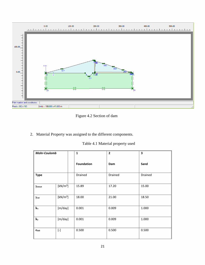
1. Section of the dam was designed by using coordinate.

21

Figure 4.2 Section of dam

2. Material Property was assigned to the different components.

Table 4.1 Material property used

Mohr-Coulomb

1

Foundation

2

Dam

3

Sand

Type Drained Drained Drained

unsat [kN/m³] 15.89 17.20 15.00

sat [kN/m³] 18.00 21.00 18.50

kx [m/day] 0.001 0.009 1.000

ky [m/day] 0.001 0.009 1.000

einit [-] 0.500 0.500 0.500

22

Mohr-Coulomb

1

Foundation

2

Dam

3

Sand

ck [-] 1E15 1E15 1E15

Eref [kN/m²] 50000.000 20000.000 20000.000

[-] 0.300 0.300 0.300

Gref [kN/m²] 19230.769 7692.308 7692.308

Eoed [kN/m²] 67307.692 26923.077 26923.077

cref [kN/m²] 32.00 38.00 2.00

[°] 15.83 12.45 35.00

[°] 0.00 0.00 0.00

Einc [kN/m²/m] 0.00 0.00 0.00

yref [m] 0.000 0.000 0.000

cincrement [kN/m²/m] 0.00 0.00 0.00

Tstr. [kN/m²] 0.00 0.00 0.00

Rinter. [-] 1.00 1.00 1.00

Interface

permeability

Neutral Neutral Neutral

23

3. Mess Generation.

Figure 4.3 Mess generation.

4. Phreatic line was drawn on the dam section.

Figure 4.4 Phreatic line.

24

CALCULATION STAGE

1. First stage of calculation was done as Plastic.

2. Second and Final stage of calculation as phi-c reduction.

Figure 4.5 Different calculation stage

POST PROCESSING

In the post processing stage, plotting of curves between various calculated parameters such

as vertical strain,shear stress,active pore water pressure,etc were obtained.It is the output

of the analysis.

4.4 SPILLWAY DESIGN:

The profile of the spillway was designed considering the discharge and the Maximum flood level.

Discharge of Ogee rested spillway is given as,

𝑄 = 𝐶. 𝐿𝑒𝐻𝑒

32⁄

25

Where, 𝐶=Coeffecient of discharge

Le=Effective length of spillway crest=120m

He=Head over the crest including velocity head and Q=Discharge

Dowstream profile:

The upstream of the spillway was asumed to be vertical and downstream face parabolic and using

WES formula,the downstream crest profile was drawan by finding the coordinate as given by,

𝑥1.85 = 2 ∗ 𝐻𝑑0.85*y

The downstream face slope was assumed to be 0.7H:1V

Upstream profile:The upstream profile was drawn by finding the coordinate using the following

formula given by U.S.Army corps,

Y=0.724(𝑥+.27𝐻𝑑)1.85

𝐻𝑑 + 0.126𝐻𝑑-0.4315𝐻𝑑

0.375(x + 0.27𝐻𝑑)0.625

Where x=-0.27𝐻𝑑

Final profile was drawn in graph by using the coordinate of upstream and downstream and was

extended to the base of the dam to give complete spillway profile.

********

26

CHAPTER 5

RESULTS AND CALCULATIONS

5.1 HYDROLOGY

5.1.1 Estimation of missing rainfall data:

The missing rainfall data were estimated by rainfall-rainfall correlation of the two station by

regression fromula in MS-EXCEL.

Table 5.1 Rainfall data of Kalyanisinghpur(in mm)

Year June July August September October

1969-70 161 420 152 126 27

1970-71 334 324 371 202 21

1971-72 216 192 278 168 151

1972-73 191 186 165 595 56

1973-74 50 404 289 83 136

1974-75 225 164 82 147 75

1975-76 328 223 242 197 40

1976-77 183 382 313 121 19

1977-78 160 528 195 268 28

1978-79 117 320 454 48 4

1979-80 270 132 117 108 37

1980-81 310 272 130 270 47

1981-82 106 148 358 380 7

27

1982-83 118 470 504 70 62

1983-84 78 164 384 414 82

1984-85 268 314 213 87 60

1985-86 215 205 334 152 60

1986-87 212 324 138 29 108

1987-88 30 177 137 120 148

1988-89 204 222 340 175 65

1989-90 397 234 282 101 10

1990-91 181 270 279 156 260

1991-92 131 561 421 175 78

1992-93 264 770 286 209 30

1993-94 169 272 136 206 48

1994-95 269 327 334 381 97

1995-96 82 331 180 155 18

1996-97 136 280 302 74 32

1997-98 181 240 357 182 17

1998-99 162 416 298 254 81

1999-00 164 172 152 239 51

2000-01 134 359 242 33 2

2001-02 375 312 220 143 32

2002-03 199 87 287 121 60

2003-04 133 311 269 218 106

28

2004-05 145 276 355 129 136

2005-06 153 213 95 343 210

2006-07 246 474 595 385 12

2007-08 357 314 666 280 56

2008-09 226 215 365 417 63

2009-10 115 651 329 184 34

Table 5.2: Rainfall data of Kashipur(in mm)

Year June July August September October

1990-91 317 389 621 189 253

1991-92 148 1262 1220 239 126

1992-93 614 924 650 345 82

1993-94 281 395 296 335 101

1994-95 634 565 839 844 137

1995-96 253 578 346 187 68

1996-97 171 418 709 111 85

1997-98 317 312 939 260 66

1998-99 262 873 695 505 127

1999-00 267 199 308 451 104

2000-01 152 495 531 183 24

2001-02 354 729 372 192 73

2002-03 149 198 585 77 129

29

2003-04 98 409 397 409 217

2004-05 459 302 747 177 103

2005-06 179 369 293 533 230

2006-07 242 968 1027 746 3

2007-08 371 306 698 420 95

2008-09 356 227 652 403 56

2009-10 30 849 814 145 152

Figure 5.1 Rainfall-Rainfall corelation for June(in mm)

y = 2.6291x - 130.8R² = 0.8132

0

100

200

300

400

500

600

700

0 50 100 150 200 250 300

Rai

nfa

ll o

f K

ash

ipu

r

Rainfall of Kalyanisinghpur

Rainfall-Rainfall corelation for june (in mm)

30

Figure 5.2 Rainfall-Rainfall corelation for July (in mm)

Figure 5.3 Rainfall-Rainfall corelation for August (in mm)

y = 1.5587x + 24.295R² = 0.706

0

200

400

600

800

1000

1200

1400

0 100 200 300 400 500 600 700 800 900

Rai

nfa

ll o

f K

ash

ipu

r

Rainfall of Kalyanisinghpur

Rainfall-Rainfall corelation for July (in mm)

y = 3.1522x - 202.99R² = 0.9686

0

200

400

600

800

1000

1200

1400

0 50 100 150 200 250 300 350 400 450

Rai

nfa

ll o

f K

ash

ipu

r

Rainfall of Kalynisinghpur

Rainfall-Rainfall corelation for August (in mm)

31

Figure 5.4 Rainfall-Rainfall corelation for September (in mm)

Figure 5.5 Rainfall-Rainfall corelation for October (in mm)

y = 2.5967x - 180.79R² = 0.9576

0

100

200

300

400

500

600

700

800

900

0 50 100 150 200 250 300 350 400 450

Rai

nfa

ll o

f K

ash

ipu

r

Rainfall of Kalyanisinghpur

Rainfall-Rainfall corelation for September(in mm)

y = 0.6502x + 78.007R² = 0.8445

0

50

100

150

200

250

300

0 50 100 150 200 250 300

Rai

nfa

ll o

f K

ash

ipu

r

Rainfall of Kalyanisinghpur

Rainfall-Rainfall corelation for October(in mm)

32

Table 5.3 Final Rainfall data of Kashipur including estimated rainfall.

Year June July August September October

1969-70 255 679 276 146 82

1970-71 971 529 966 344 77

1971-72 427 324 673 255 175

1972-73 347 314 317 1364 103

1973-74 66 654 708 35 164

1974-75 457 280 55 201 118

1975-76 940 372 560 331 91

1976-77 323 620 784 133 75

1977-78 254 847 412 515 82

1978-79 83 523 1228 6 64

1979-80 639 230 166 100 89

1980-81 847 448 207 520 97

1981-82 21 255 925 806 66

1982-83 89 757 1386 1 108

1983-84 54 280 1007 894 123

1984-85 630 514 468 45 106

1985-86 422 344 850 214 106

1986-87 411 529 232 5 143

1987-88 21 300 229 131 173

1988-89 386 370 869 274 110

1989-90 1222 389 686 81 69

1990-91 317 389 621 189 253

1991-92 148 1262 1220 239 126

33

1992-93 614 924 650 345 82

1993-94 281 395 296 335 101

1994-95 634 565 839 844 137

1995-96 253 578 346 187 68

1996-97 171 418 709 111 85

1997-98 317 312 939 260 66

1998-99 262 873 695 505 127

1999-00 267 199 308 451 104

2000-01 152 495 531 183 24

2001-02 354 729 372 192 73

2002-03 149 198 585 77 129

2003-04 98 409 397 409 217

2004-05 459 302 747 177 103

2005-06 179 369 293 533 230

2006-07 242 968 1027 746 3

2007-08 371 306 698 420 95

2008-09 356 227 652 403 56

2009-10 30 849 814 145 152

5.1.2 Mean Aerial Rainfall:

Using thiessen polygon method mean precipitation was obtained.

Influence factor or Thiessen weight for Kalyanisinghpur and Lanjigarh = 0.591+0.132= 0.723

Thiessen weight for Kashipur and Thumal Rampur =0.2045+0.072= 0.2765

This thiessen weight was used to compute the mean aerial rainfall.

34

Table 5.4 Mean Monthly Rainfall (in mm)

Year June July August September October

1969-70 187 491 186 131 42

1970-71 510 381 535 241 36

1971-72 274 228 387 192 158

1972-73 234 221 207 807 69

1973-74 54 473 405 70 144

1974-75 289 196 74 162 87

1975-76 497 264 330 234 54

1976-77 222 448 443 124 34

1977-78 186 616 255 336 43

1978-79 108 376 668 36 21

1979-80 372 159 130 106 51

1980-81 458 321 151 339 61

1981-82 82 178 515 498 23

1982-83 110 549 748 51 75

1983-84 71 196 556 547 93

1984-85 368 369 283 75 73

1985-86 272 243 477 169 73

1986-87 267 381 164 22 118

1987-88 27 211 162 123 155

1988-89 254 263 486 202 77

1989-90 625 277 394 95 26

1990-91 219 303 373 165 258

1991-92 136 755 642 193 91

35

1992-93 361 812 387 246 44

1993-94 200 306 180 242 63

1994-95 370 393 473 509 108

1995-96 129 399 226 164 32

1996-97 146 318 414 84 47

1997-98 219 260 518 203 31

1998-99 190 542 408 323 94

1999-00 192 179 195 297 66

2000-01 139 396 322 74 8

2001-02 369 427 262 156 43

2002-03 185 118 369 109 79

2003-04 123 338 304 271 137

2004-05 232 283 463 142 127

2005-06 160 256 150 395 215

2006-07 245 610 714 485 10

2007-08 361 312 675 319 67

2008-09 262 218 444 413 61

2009-10 91 705 463 173 67

5.1.3 Synthetic Unit Hydrograph:

Catchment Area= 1176 sq. km

L=78 km

Lc= 31.76 km

Ct for the catchment =1.35

36

Lag Time, tp:-

tp = C

t (L.L

c)0.3

=14.077 hours

Duration of Rainfall excess, tre

:-

tre

= tp / 5.5 =2.56<4 hours.

Modified lag time taking duration of rainfall excess, tr = 4 hours

tnp

= tp + 0.25 (t

r - t

re) =14.437 hours

Peak Discharge:-

𝑄𝑝𝑟 =2.78𝐶𝑃𝐴

𝑡𝑝

= (2.78 x .56 x 1176)/14.437

=126.81cumecs.

Time base:-

𝑇𝑏 =5(𝑡𝑛𝑝+ .5𝑡𝑟) = 79.68 hours

UH Widths:-

𝑊50 =5.87

𝑞𝑝𝑟𝑢1.08 = 65.05 ; (𝑞𝑝𝑟𝑢 =

𝑄𝑝𝑟

𝐴 =0.107 )

𝑊75 =3.354

𝑞𝑝𝑟𝑢1.08 = 37.17

Usually, 1/3 of the width is distributed before UH peak and 2/3 after the peak. The volume of

37

UH was checked and was corrected to be close to 1 cm 1 cm x area of the catchment in 𝑘𝑚2.

Thus from the above equations the synthetic unit hydrograph was drawn as shown below.

Figure 5.6 Syntheti Unit Hydrograph

0

20

40

60

80

100

120

140

0 20 40 60 80 100 120

Dis

char

ge (

in c

um

ecs)

Time (in hours)

39

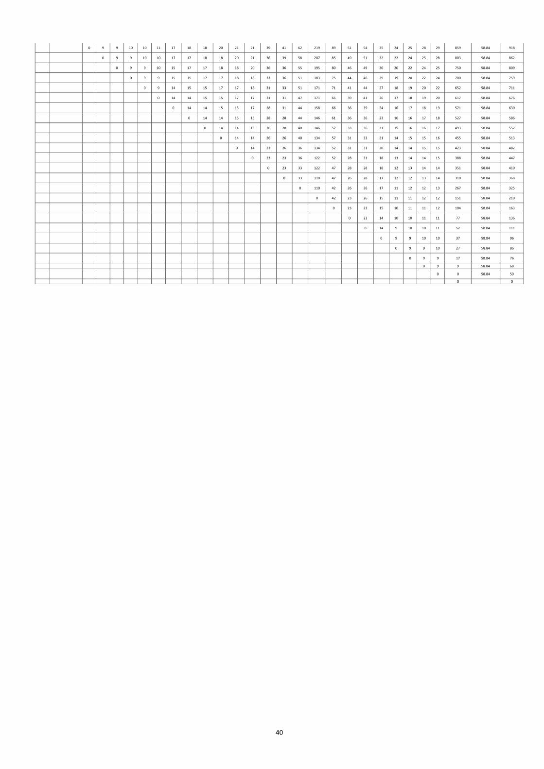
5.1.4 Flood Hydrograph or Design Flood:

Time Discharge Ordinate

RAINFALL EXCESS(mms/cms)

9.68 9.68 9.69 9.69 9.69 9.69 15.03 15.03 15.04 15.04 15.04 15.04 25.72 25.72 36.41 121.92 47.09 25.72 25.72 15.03 9.69 9.69 9.68 9.68 Surface Runoff

Base Flow @0.05

cum/sq km

Total Runoff

0.97 0.97 0.97 0.97 0.97 0.97 1.5 1.5 1.5 1.5 1.5 1.5 2.57 2.57 3.64 12.19 4.71 2.57 2.57 1.5 0.97 0.97 0.97 0.97

0 0 0 0 58.84 59

1 1 1 0 1 58.84 60

2 4 4 1 0 5 58.84 64

3 5 5 4 1 0 10 58.84 69

4 9 9 5 4 1 0 18 58.84 77

5 12 12 9 5 4 1 0 30 58.84 89

6 20 19 12 9 5 4 1 0 49 58.84 108

7 35 34 19 12 9 5 4 2 0 84 58.84 143

8 60 58 34 19 12 9 5 6 2 0 144 58.84 203

9 90 87 58 34 19 12 9 8 6 2 0 234 58.84 293

10 117 113 87 58 34 19 12 14 8 6 2 0 352 58.84 411

11 121 117 113 87 58 34 19 18 14 8 6 2 0 476 58.84 534

12 125 121 117 113 87 58 34 30 18 14 8 6 2 0 607 58.84 666

13 127 123 121 117 113 87 58 53 30 18 14 8 6 3 0 750 58.84 809

14 128 124 123 121 117 113 87 90 53 30 18 14 8 10 3 0 911 58.84 969

15 128 124 124 123 121 117 113 135 90 53 30 18 14 13 10 4 0 1089 58.84 1148

16 126 122 124 124 123 121 117 176 135 90 53 30 18 23 13 15 12 0 1296 58.84 1355

17 123 119 122 124 124 123 121 182 176 135 90 53 30 31 23 18 49 5 0 1525 58.84 1584

18 121 117 119 122 124 124 123 188 182 176 135 90 53 51 31 33 61 19 3 0 1751 58.84 1810

19 120 116 117 119 122 124 124 191 188 182 176 135 90 90 51 44 110 24 10 3 0 2016 58.84 2075

20 116 112 116 117 119 122 124 192 191 188 182 176 135 154 90 73 146 42 13 10 2 0 2306 58.84 2365

21 112 108 112 116 117 119 122 192 192 191 188 182 176 231 154 127 244 57 23 13 6 1 0 2674 58.84 2733

22 106 103 108 112 116 117 119 189 192 193 191 188 182 301 231 218 427 94 31 23 8 4 1 0 3150 58.84 3208

23 100 97 103 109 112 116 117 185 189 193 193 191 188 311 301 328 732 165 51 31 14 5 4 1 0 3734 58.84 3793

24 95 92 97 103 109 112 116 182 185 190 193 193 191 322 311 426 1097 283 90 51 18 9 5 4 1 4377 58.84 4436

25 90 87 92 97 103 109 112 180 182 185 190 193 193 327 322 441 1426 424 154 90 30 12 9 5 4 4964 58.84 5023

26 81 78 87 92 97 103 109 174 180 182 185 190 193 329 327 455 1475 551 231 154 53 19 12 9 5 5290 58.84 5348

27 77 75 78 87 92 97 103 168 174 180 182 185 190 329 329 462 1524 570 301 231 90 34 19 12 9 5522 58.84 5581

28 73 71 75 78 87 92 97 159 168 174 180 182 185 324 329 466 1548 589 311 301 135 58 34 19 12 5676 58.84 5735

29 70 68 71 75 78 87 92 150 159 168 174 180 182 316 324 466 1561 598 322 311 176 87 58 34 19 5758 58.84 5817

30 65 63 68 71 75 78 87 143 150 159 168 174 180 311 316 459 1561 603 327 322 182 113 87 58 34 5790 58.84 5849

31 59 57 63 68 71 75 78 135 143 150 159 168 174 309 311 448 1536 603 329 327 188 117 113 87 58 5769 58.84 5828

32 55 53 57 63 68 71 75 122 135 143 150 159 168 298 309 441 1500 593 329 329 191 121 117 113 87 5693 58.84 5752

33 50 48 53 57 63 68 71 116 122 135 143 150 159 288 298 437 1475 579 324 329 192 123 121 117 113 5584 58.84 5643

34 45 44 48 53 57 63 68 110 116 122 135 143 150 273 288 422 1463 570 316 324 192 124 123 121 117 5443 58.84 5502

35 42 41 44 48 53 57 63 105 110 116 122 135 143 257 273 408 1414 565 311 316 189 124 124 123 121 5263 58.84 5322

36 39 38 41 44 48 53 57 98 105 110 116 122 135 244 257 386 1366 546 309 311 185 122 124 124 123 5064 58.84 5122

37 35 34 38 41 44 48 53 89 98 105 110 116 122 231 244 364 1292 527 298 309 182 119 122 124 124 4834 58.84 4893

38 33 32 34 38 41 44 48 83 89 98 105 110 116 208 231 346 1219 499 288 298 180 117 119 122 124 4589 58.84 4648

39 30 29 32 34 38 41 44 75 83 89 98 105 110 198 208 328 1158 471 273 288 174 116 117 119 122 4349 58.84 4408

40 29 28 29 32 34 38 41 68 75 83 89 98 105 188 198 295 1097 447 257 273 168 112 116 117 119 4107 58.84 4166

41 26 25 28 29 32 34 38 63 68 75 83 89 98 180 188 280 988 424 244 257 159 109 112 116 117 3836 58.84 3895

42 25 24 25 28 29 32 34 59 63 68 75 83 89 167 180 266 939 381 231 244 150 103 109 112 116 3608 58.84 3666

43 23 22 24 25 28 29 32 53 59 63 68 75 83 152 167 255 890 363 208 231 143 97 103 108 112 3390 58.84 3449

44 21 20 22 24 25 28 29 50 53 59 63 68 75 141 152 237 853 344 198 208 135 92 97 103 108 3185 58.84 3244

45 20 19 20 22 24 25 28 45 50 53 59 63 68 129 141 215 792 330 188 198 122 87 92 97 103 2970 58.84 3028

46 19 18 19 20 22 24 25 44 45 50 53 59 63 116 129 200 719 306 180 188 116 78 87 92 97 2751 58.84 2809

47 18 17 18 19 20 22 24 39 44 45 50 53 59 108 116 182 671 278 167 180 110 75 78 87 92 2554 58.84 2613

48 17 16 17 18 19 20 22 38 39 44 45 50 53 100 108 164 610 259 152 167 105 71 75 78 87 2358 58.84 2417

49 16 15 16 17 18 19 20 35 38 39 44 45 50 90 100 153 549 235 141 152 98 68 71 75 78 2167 58.84 2226

50 15 15 15 16 17 18 19 32 35 38 39 44 45 85 90 142 512 212 129 141 89 63 68 71 75 2009 58.84 2068

51 14 14 15 16 16 17 18 30 32 35 38 39 44 77 85 127 475 198 116 129 83 57 63 68 71 1861 58.84 1920

52 14 14 14 15 16 16 17 29 30 32 35 38 39 75 77 120 427 184 108 116 75 53 57 63 68 1715 58.84 1774

53 13 13 14 14 15 16 16 27 29 30 32 35 38 67 75 109 402 165 100 108 68 48 53 57 63 1591 58.84 1650

54 12 12 13 14 14 15 16 26 27 29 30 32 35 64 67 106 366 155 90 100 63 44 48 53 57 1473 58.84 1531

55 12 12 12 13 14 14 15 24 26 27 29 30 32 59 64 95 354 141 85 90 59 41 44 48 53 1377 58.84 1436

56 11 11 12 12 13 14 14 23 24 26 27 29 30 54 59 91 317 137 77 85 53 38 41 44 48 1274 58.84 1333

57 11 11 11 12 12 13 14 21 23 24 26 27 29 51 54 84 305 122 75 77 50 34 38 41 44 1193 58.84 1252

58 10 10 11 11 12 12 13 21 21 23 24 26 27 49 51 76 280 118 67 75 45 32 34 38 41 1114 58.84 1173

59 10 10 10 11 11 12 12 20 21 21 23 24 26 46 49 73 256 108 64 67 44 29 32 34 38 1038 58.84 1096

60 9 9 10 10 11 11 12 18 20 21 21 23 24 44 46 69 244 99 59 64 39 28 29 32 34 975 58.84 1034

61 9 9 9 10 10 11 11 18 18 20 21 21 23 41 44 66 232 94 54 59 38 25 28 29 32 920 58.84 979

40

0 9 9 10 10 11 17 18 18 20 21 21 39 41 62 219 89 51 54 35 24 25 28 29 859 58.84 918

0 9 9 10 10 17 17 18 18 20 21 36 39 58 207 85 49 51 32 22 24 25 28 803 58.84 862

0 9 9 10 15 17 17 18 18 20 36 36 55 195 80 46 49 30 20 22 24 25 750 58.84 809

0 9 9 15 15 17 17 18 18 33 36 51 183 75 44 46 29 19 20 22 24 700 58.84 759

0 9 14 15 15 17 17 18 31 33 51 171 71 41 44 27 18 19 20 22 652 58.84 711

0 14 14 15 15 17 17 31 31 47 171 66 39 41 26 17 18 19 20 617 58.84 676

0 14 14 15 15 17 28 31 44 158 66 36 39 24 16 17 18 19 571 58.84 630

0 14 14 15 15 28 28 44 146 61 36 36 23 16 16 17 18 527 58.84 586

0 14 14 15 26 28 40 146 57 33 36 21 15 16 16 17 493 58.84 552

0 14 14 26 26 40 134 57 31 33 21 14 15 15 16 455 58.84 513

0 14 23 26 36 134 52 31 31 20 14 14 15 15 423 58.84 482

0 23 23 36 122 52 28 31 18 13 14 14 15 388 58.84 447

0 23 33 122 47 28 28 18 12 13 14 14 351 58.84 410

0 33 110 47 26 28 17 12 12 13 14 310 58.84 368

0 110 42 26 26 17 11 12 12 13 267 58.84 325

0 42 23 26 15 11 11 12 12 151 58.84 210

0 23 23 15 10 11 11 12 104 58.84 163

0 23 14 10 10 11 11 77 58.84 136

0 14 9 10 10 11 52 58.84 111

0 9 9 10 10 37 58.84 96

0 9 9 10 27 58.84 86

0 9 9 17 58.84 76

0 9 9 58.84 68

0 0 58.84 59

0 0

41

5.2 Cross-section of Dam:

Considering the recommendation of IS 8826 : 1978 Guidelines for design of large earth and

rockfill dams and Geotechnical properties crossection of dam was designed.

42

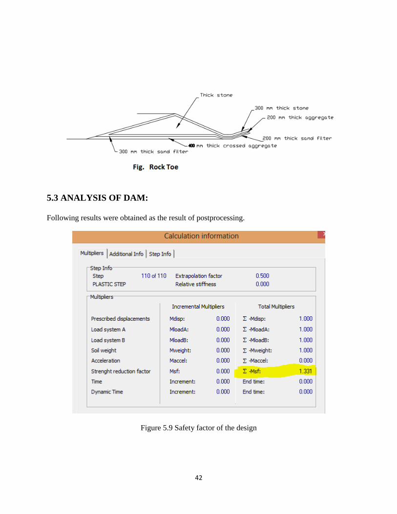
5.3 ANALYSIS OF DAM:

Following results were obtained as the result of postprocessing.

Figure 5.9 Safety factor of the design

43

Figure 5.10 Active pore pressure

Figure 5.11.Horizontal Total Stress

44

Figure 5.12 Horizontal effective stress.

Figure 5.13 Vertical Strain

45

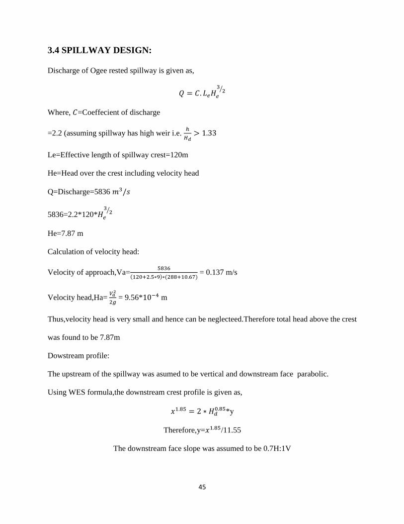
3.4 SPILLWAY DESIGN:

Discharge of Ogee rested spillway is given as,

𝑄 = 𝐶. 𝐿𝑒𝐻𝑒

32⁄

Where, 𝐶=Coeffecient of discharge

=2.2 (assuming spillway has high weir i.e. ℎ

𝐻𝑑> 1.33

Le=Effective length of spillway crest=120m

He=Head over the crest including velocity head

Q=Discharge=5836 𝑚3/𝑠

5836=2.2*120*𝐻𝑒

32⁄

He=7.87 m

Calculation of velocity head:

Velocity of approach,Va=5836

(120+2.5∗9)∗(288+10.67) = 0.137 m/s

Velocity head,Ha= 𝑉𝑎

2

2𝑔 = 9.56*10−4 m

Thus,velocity head is very small and hence can be neglecteed.Therefore total head above the crest

was found to be 7.87m

Dowstream profile:

The upstream of the spillway was asumed to be vertical and downstream face parabolic.

Using WES formula,the downstream crest profile is given as,

𝑥1.85 = 2 ∗ 𝐻𝑑0.85*y

Therefore,y=𝑥1.85/11.55

The downstream face slope was assumed to be 0.7H:1V

46

𝑑𝑦

𝑑𝑥=

1

0.7

Therefore ,x=13.12 m and y= 7.82 m.

The tangent point is at (13.12,7.82)

Table. 5.6 Various coordinates of downstream profile.

x y

1 0.08658

2 0.312121

3 0.660834

4 1.125198

5 1.700249

6 2.382308

7 3.168468

8 4.056341

9 5.043902

10 6.129401

11 7.311298

12 8.588223

13 9.958942

13.12 10.12968

Upstream profile:

Y=0.724(𝑥+.27𝐻𝑑)1.85

𝐻𝑑 + 0.126𝐻𝑑-0.4315𝐻𝑑

0.375(x + 0.27𝐻𝑑)0.625

Where x=-0.27𝐻𝑑= 2.12

Table 5.7 Various coordinates of upstream profile.

x y

-0.5 0.04943

-1 0.099253

-1.5 0.332976

-2 0.738708

-2.12 0.957947

Final profile was drawn in graph by using the coordinate of upstream and downstream and was

extended to the base of the dam to give complete spillway profile.

47

Figure 5.14 Profile of Spillway

48

CHAPTER 6

CONCLUSIONS

The dam constructed when analysed using PLAXIS gave the safety factor of 1.33 and hence the

dam was found to safe against over all stability. From this paper it can be concluded that for a

design of any dam, hydrological features must be properly studied before designing to ensure the

safety and PLAXIS softwarecan be used for the accurate analysis any Earth dam.

49

REFERENCES

[1] George H. Hargreaves; Gary P. Merkley, Irrigation Fundamentals, Water Resources

Publications, LLC, 1998, pp. 2.

[2] Duo, Esther, and Pande,Rohini,Draft :July 2005, “Dams.”

[3] Singh V. P.,Dam Breach Modelling Technology,Kluwer academic publishers,pg 88-89.

[4]Patra, K.C., Hydrology and Water Resources Engineering, 2012, Second Edition,Narosa

Publication, pp. 334.

[5] Snyder, F. F. 1938. Synthetic Unit-Graphs. Transactions, American Geophysical Union, 19,

447-454.

[6] http://www.britannica.com/EBchecked/topic/559952/spillway DOA-15th march 2013

[7] Y.Q. Xu, Unami K. and Kawachi T., January 2003, Optimal hydraulic design of earth dam

cross section using saturated–unsaturated seepage flow model.

[8] Tien-kuen Hnang, 17 March 1996 “Stability analysis of an earth dam under steady state

seepage”

[9] Abolfazl Nazari Giglou, Taher Nazari Giglou and Afshar Minaei, 2013, “Seepage through

Earth Dam”

[10] Rasul Daneshfaraz1, Shabnam Vakili, Mahdi Majedi-Asl and Mohammad Rostami, 2012,

“Numerical Investigation of Upstream Face Slope and Curvature of Ogee Spillway on Flow

Pattern”, Journal of Environmental Science and Engineering.

[11] Garg, S.K., Irrigation Engineering and Hydraulic Structures(2011), 24th edition, Khanna

Publishers.

[12] IS 10635 : 1993 Freeboard requirements in embankment dams – Guidelines

[13] IS 8826 : 1978 Guidelines for design of large earth and rockfill dams

50