design and implementation of a simulator for …paupo/publications... · design and implementation...
TRANSCRIPT

Design and Implementation of a Simulator forMeasuring the Quality of Service forDistributed Multimedia Applications
Rolf Esbjørn Kristensen
Kongens Lyngby 2009IMM-M.Sc.-2009-XX
Draft

Technical University of DenmarkInformatics and Mathematical ModellingBuilding 321, DK-2800 Kongens Lyngby, DenmarkPhone +45 45253351, Fax +45 [email protected]
IMM-M.Sc.: ISSN XXXX-XXXX

Abstract
Multimedia applications have become widespread today, from streaming over theInternet to portable music and video players. Increasingly multimedia applicationsare implemented using embedded architectures, which have very tight constraints interms of cost, performance, power consumption, size, etc. Examples of such systemsare smart-phones, an iPod or a TV set-top-box.
Designing embedded systems implementing multimedia applications is difficult be-cause of the inherent variability of functionality execution times (which depend onthe video or audio streams processed, their resolution, frame rate, etc.) and stringentQuality-of-Service (QoS) requirements on their performance (e.g., a playback of 25frames per second for a video device).
Real-time systems theory provides analysis methods that can determine if an appli-cation implemented on an embedded architecture meets its timing constraints. Thereare a lot of results for hard real-time systems, which have to meet their deadlineseven in the worst-case, otherwise something catastrophic can happen. In contrast,a multimedia application is a soft real-time system, where certain degradation ofperformance can be accepted, provided it is not below a given level of QoS.
Multimedia systems are difficult to analyse using existing schedulability analysistheory. Designing an architecture based on the worst-case leads to over design: toomuch computing power, which is seldom used. Hence, the focus of this thesis is toimplement a simulator that can support the designer in evaluating very early in thedevelopment process several embedded architecture implementations, and decidingwhich one meets the QoS requirements for a given multimedia application. This canreduce the time-to-market and development costs by avoiding building a physicalprototype, which is costly and time-consuming.
Besides evaluating hardware architectures (CPUs, dedicated hardware, buses), we arealso interested in using the simulator to evaluate several scheduling policies, whichhave a strong impact on the behaviour of the application. Our simulator, whichis based on the SystemC library, can take into account Fixed-Priority preemptivescheduling (FP), Earliest Deadline First scheduling (EDF), the Linux 2.6 schedulerand Constant-Bandwidth Server scheduling (CBS). The idea of the CBS is to dividea resource (CPU or bus) into virtual resources, which are given a certain budget.This is especially useful if several applications (both hard and soft real-time) haveto share the same architecture.
The simulator has been used to evaluate several architecture alternatives for a set-top-box application, using different hardware components and scheduling policies.
iii

Chapter 0. Abstract
As the experiments show, using the simulator we can chose very quickly the rightarchitecture and scheduling policy. The simulator can also help in deciding thescheduling parameters, such as the bandwidth for the CBS servers.
iv

Resumé
!!! Danish abstract !!!
v

Chapter 0. Resumé
vi

Preface
This master thesis was written at the department of Informatics and MathematicalModelling at the Technical University of Denmark DTU. The project was completedin the period September 2008 to March 2009, under the supervision of associateprofessor Paul Pop. The thesis is a 30 ECTS point course.
I would like to thank Paul Pop, and Ph.d. Prabhat Kumar Saraswat for guidanceand support throughout the project. I would also like to thank my father and SuneJakobsen for proofreading the thesis.
Rolf Esbjørn [email protected]
Kongens Lyngby, March 2009
vii

Chapter 0. Preface
viii

Contents
Abstract iii
Resumé v
Preface vii
Abbreviations xiii
1 Introduction 11.1 Variability in Multimedia . . . . . . . . . . . . . . . . . . . . . . . . 21.2 Motivation . . . . . . . . . . . . . . . . . . . . . . . . . . . . . . . . . 31.3 Related work . . . . . . . . . . . . . . . . . . . . . . . . . . . . . . . 31.4 My work throughout the thesis . . . . . . . . . . . . . . . . . . . . . 41.5 Structure of the thesis . . . . . . . . . . . . . . . . . . . . . . . . . . 5
2 Multimedia 72.1 Types of Multimedia . . . . . . . . . . . . . . . . . . . . . . . . . . . 7
2.1.1 MPEG . . . . . . . . . . . . . . . . . . . . . . . . . . . . . . . 72.1.2 MP3 . . . . . . . . . . . . . . . . . . . . . . . . . . . . . . . . 11
2.2 Metrics . . . . . . . . . . . . . . . . . . . . . . . . . . . . . . . . . . 132.3 Variability in multimedia . . . . . . . . . . . . . . . . . . . . . . . . . 15
2.3.1 Modelling the variability . . . . . . . . . . . . . . . . . . . . . 172.4 Distributed Multimedia . . . . . . . . . . . . . . . . . . . . . . . . . 182.5 Scheduling . . . . . . . . . . . . . . . . . . . . . . . . . . . . . . . . . 19
2.5.1 Fixed priority scheduling . . . . . . . . . . . . . . . . . . . . . 192.5.2 Earliest Deadline First . . . . . . . . . . . . . . . . . . . . . . 202.5.3 Constant bandwidth server scheduling . . . . . . . . . . . . . 202.5.4 Linux scheduler . . . . . . . . . . . . . . . . . . . . . . . . . . 222.5.5 Hypothesis . . . . . . . . . . . . . . . . . . . . . . . . . . . . 23
3 Simulators 253.1 Levels of Abstraction . . . . . . . . . . . . . . . . . . . . . . . . . . . 263.2 Design-Level Simulator . . . . . . . . . . . . . . . . . . . . . . . . . . 273.3 Existing Simulators . . . . . . . . . . . . . . . . . . . . . . . . . . . . 28
3.3.1 SimpleScalar . . . . . . . . . . . . . . . . . . . . . . . . . . . 283.3.2 Simics . . . . . . . . . . . . . . . . . . . . . . . . . . . . . . . 29
ix

Contents
3.3.3 PTLsim . . . . . . . . . . . . . . . . . . . . . . . . . . . . . . 303.3.4 SystemC . . . . . . . . . . . . . . . . . . . . . . . . . . . . . . 303.3.5 Pesimdes . . . . . . . . . . . . . . . . . . . . . . . . . . . . . 313.3.6 ARTS . . . . . . . . . . . . . . . . . . . . . . . . . . . . . . . 313.3.7 Summary . . . . . . . . . . . . . . . . . . . . . . . . . . . . . 32
4 Design of the Simulator 334.1 What needs to be simulated . . . . . . . . . . . . . . . . . . . . . . . 334.2 Requirements . . . . . . . . . . . . . . . . . . . . . . . . . . . . . . . 344.3 PESIMDES . . . . . . . . . . . . . . . . . . . . . . . . . . . . . . . . 354.4 Structure of the simulator . . . . . . . . . . . . . . . . . . . . . . . . 36
4.4.1 Scheduling . . . . . . . . . . . . . . . . . . . . . . . . . . . . . 374.4.1.1 Fixed priority scheduling . . . . . . . . . . . . . . . 394.4.1.2 Earliest Deadline First scheduling . . . . . . . . . . 404.4.1.3 Constant bandwidth server scheduling . . . . . . . . 404.4.1.4 Linux scheduler . . . . . . . . . . . . . . . . . . . . 41
4.4.2 Input and output . . . . . . . . . . . . . . . . . . . . . . . . . 42
5 Implementation of the Simulator 435.1 Communication . . . . . . . . . . . . . . . . . . . . . . . . . . . . . . 435.2 Scheduling . . . . . . . . . . . . . . . . . . . . . . . . . . . . . . . . . 46
5.2.1 Fixed-Priority . . . . . . . . . . . . . . . . . . . . . . . . . . . 485.2.2 Earliest Deadline First . . . . . . . . . . . . . . . . . . . . . . 495.2.3 Constant Bandwidth Server . . . . . . . . . . . . . . . . . . . 515.2.4 Linux O(1) . . . . . . . . . . . . . . . . . . . . . . . . . . . . 54
5.3 Output devices . . . . . . . . . . . . . . . . . . . . . . . . . . . . . . 555.3.1 Consumer . . . . . . . . . . . . . . . . . . . . . . . . . . . . . 565.3.2 Output display . . . . . . . . . . . . . . . . . . . . . . . . . . 57
5.4 Extending DiMAS . . . . . . . . . . . . . . . . . . . . . . . . . . . . 57
6 Generating traces for the simulator 596.1 Resulting trace files . . . . . . . . . . . . . . . . . . . . . . . . . . . . 61
7 Case studies 637.1 Evaluation criteria . . . . . . . . . . . . . . . . . . . . . . . . . . . . 637.2 Reading this chapter . . . . . . . . . . . . . . . . . . . . . . . . . . . 647.3 General set-up . . . . . . . . . . . . . . . . . . . . . . . . . . . . . . 647.4 Two processing elements . . . . . . . . . . . . . . . . . . . . . . . . . 66
7.4.1 Case study 1 - Periodic input . . . . . . . . . . . . . . . . . . 667.4.1.1 Test bench . . . . . . . . . . . . . . . . . . . . . . . 677.4.1.2 TC 1.0 - FP . . . . . . . . . . . . . . . . . . . . . . 677.4.1.3 TC 1.1 - EDF . . . . . . . . . . . . . . . . . . . . . 687.4.1.4 TC 1.2 - EDF+CBS . . . . . . . . . . . . . . . . . . 697.4.1.5 TC 1.3 - Linux . . . . . . . . . . . . . . . . . . . . . 707.4.1.6 Summary . . . . . . . . . . . . . . . . . . . . . . . . 70
7.4.2 Case study 2 - GUI task . . . . . . . . . . . . . . . . . . . . . 73
x

Contents
7.4.2.1 Test bench . . . . . . . . . . . . . . . . . . . . . . . 737.4.2.2 TC 2.0 - FP . . . . . . . . . . . . . . . . . . . . . . 747.4.2.3 TC 2.1 - EDF . . . . . . . . . . . . . . . . . . . . . 757.4.2.4 TC 2.2 - EDF+CBS . . . . . . . . . . . . . . . . . . 757.4.2.5 TC 2.3 - Linux . . . . . . . . . . . . . . . . . . . . . 767.4.2.6 Summary . . . . . . . . . . . . . . . . . . . . . . . . 77
7.4.3 Case study 3 - Input with jitter . . . . . . . . . . . . . . . . . 807.4.3.1 Test bench . . . . . . . . . . . . . . . . . . . . . . . 807.4.3.2 TC 3.0 - FP . . . . . . . . . . . . . . . . . . . . . . 807.4.3.3 TC 3.1 - EDF . . . . . . . . . . . . . . . . . . . . . 807.4.3.4 TC 3.2 - EDF+CBS . . . . . . . . . . . . . . . . . . 817.4.3.5 TC 3.3 - Linux . . . . . . . . . . . . . . . . . . . . . 817.4.3.6 Summary . . . . . . . . . . . . . . . . . . . . . . . . 82
7.4.4 Case study 4 - Varying CBS parameters . . . . . . . . . . . . 847.4.4.1 TC4.0 . . . . . . . . . . . . . . . . . . . . . . . . . . 857.4.4.2 TC4.1 . . . . . . . . . . . . . . . . . . . . . . . . . . 857.4.4.3 TC4.2 . . . . . . . . . . . . . . . . . . . . . . . . . . 857.4.4.4 TC4.3 . . . . . . . . . . . . . . . . . . . . . . . . . . 867.4.4.5 TC4.4 . . . . . . . . . . . . . . . . . . . . . . . . . . 867.4.4.6 Summary . . . . . . . . . . . . . . . . . . . . . . . . 86
7.5 One processing element . . . . . . . . . . . . . . . . . . . . . . . . . 887.5.1 Case study 5 - Periodic input . . . . . . . . . . . . . . . . . . 89
7.5.1.1 Test bench . . . . . . . . . . . . . . . . . . . . . . . 897.5.1.2 TC5.0 - FP . . . . . . . . . . . . . . . . . . . . . . . 897.5.1.3 TC5.1 - EDF . . . . . . . . . . . . . . . . . . . . . . 907.5.1.4 TC5.2 - EDF+CBS . . . . . . . . . . . . . . . . . . 907.5.1.5 TC5.3 - Linux . . . . . . . . . . . . . . . . . . . . . 917.5.1.6 Summary . . . . . . . . . . . . . . . . . . . . . . . . 92
7.5.2 Case study 6 - GUI task . . . . . . . . . . . . . . . . . . . . . 947.5.2.1 Test bench . . . . . . . . . . . . . . . . . . . . . . . 947.5.2.2 TC6.0 - FP . . . . . . . . . . . . . . . . . . . . . . . 947.5.2.3 TC6.1 - EDF . . . . . . . . . . . . . . . . . . . . . . 957.5.2.4 TC6.2 - EDF+CBS . . . . . . . . . . . . . . . . . . 967.5.2.5 TC6.3 - Linux . . . . . . . . . . . . . . . . . . . . . 967.5.2.6 Summary . . . . . . . . . . . . . . . . . . . . . . . . 97
7.5.3 Case study 7 - Input with jitter . . . . . . . . . . . . . . . . . 997.5.3.1 TC7.0 - FP . . . . . . . . . . . . . . . . . . . . . . . 997.5.3.2 TC7.1 - EDF . . . . . . . . . . . . . . . . . . . . . . 997.5.3.3 TC7.2 - EDF+CBS . . . . . . . . . . . . . . . . . . 1007.5.3.4 TC7.3 - Linux . . . . . . . . . . . . . . . . . . . . . 1007.5.3.5 Summary . . . . . . . . . . . . . . . . . . . . . . . . 101
7.5.4 Case study 8 - Varying CBS parameters . . . . . . . . . . . . 1037.5.4.1 TC8.0 . . . . . . . . . . . . . . . . . . . . . . . . . . 1037.5.4.2 TC8.1 . . . . . . . . . . . . . . . . . . . . . . . . . . 1047.5.4.3 TC8.2 . . . . . . . . . . . . . . . . . . . . . . . . . . 104
xi
Contents
7.5.4.4 TC8.3 . . . . . . . . . . . . . . . . . . . . . . . . . . 1047.5.4.5 TC8.4 . . . . . . . . . . . . . . . . . . . . . . . . . . 1057.5.4.6 TC8.5 . . . . . . . . . . . . . . . . . . . . . . . . . . 1057.5.4.7 Summary . . . . . . . . . . . . . . . . . . . . . . . . 105
7.6 Conclusion . . . . . . . . . . . . . . . . . . . . . . . . . . . . . . . . . 106
8 Conclusion 1098.1 Future work . . . . . . . . . . . . . . . . . . . . . . . . . . . . . . . . 110
Bibliography 111
A Developed utilities 113A.1 BreakDiff . . . . . . . . . . . . . . . . . . . . . . . . . . . . . . . . . 113A.2 mpeg2stat . . . . . . . . . . . . . . . . . . . . . . . . . . . . . . . . . 113A.3 VCD Parser . . . . . . . . . . . . . . . . . . . . . . . . . . . . . . . . 114
B Input generator class diagram 115
C Users guide 117
D Multimedia data files 123D.1 MPEG-2 files . . . . . . . . . . . . . . . . . . . . . . . . . . . . . . . 123
E Commands for generating traces 127
F Profiling two MPEG video files 129F.1 flwr_080 . . . . . . . . . . . . . . . . . . . . . . . . . . . . . . . . . . 129F.2 high_25fps_320x240 . . . . . . . . . . . . . . . . . . . . . . . . . . . 130
G CD-rom contents 133
H Case Study plots 135H.1 Variability in the MPEG video files . . . . . . . . . . . . . . . . . . . 135H.2 Case study 1 . . . . . . . . . . . . . . . . . . . . . . . . . . . . . . . 138H.3 Case study 2 . . . . . . . . . . . . . . . . . . . . . . . . . . . . . . . 146H.4 Case study 3 . . . . . . . . . . . . . . . . . . . . . . . . . . . . . . . 154H.5 Case study 4 . . . . . . . . . . . . . . . . . . . . . . . . . . . . . . . 162H.6 Case study 5 . . . . . . . . . . . . . . . . . . . . . . . . . . . . . . . 167H.7 Case study 6 . . . . . . . . . . . . . . . . . . . . . . . . . . . . . . . 175H.8 Case study 7 . . . . . . . . . . . . . . . . . . . . . . . . . . . . . . . 183H.9 Case study 8 . . . . . . . . . . . . . . . . . . . . . . . . . . . . . . . 191H.10 APE3 histogram . . . . . . . . . . . . . . . . . . . . . . . . . . . . . 197
xii

Abbreviations
API Application Programming Interface
ASIC Application-Specific Integrated Circuit
CAS Cycle-Accurate Simulator
DCT Discrete Cosine Transformation
DiMAS Distributed Multimedia Application Simulation API
FIFO First In First Out
IDCT Inverse Discrete Cosine Transformation
ISA Instruction Set Architecture
ISS Instruction Set Simulator
MP Motion compensation Prediction
MPSoC Multi Processor System-on-Chip
Pe Processing Element
RTL Register Transfer Level
SAM System Architectural Model
TLM Transaction Level Modelling
VCD Value Change Dump
vLan Virtual Local Area Network
VLC Variable Length Coding
VLD Variable Length Decoding
VoIP Voice over Internet Protocol
WiFi Wireless Fidelity
xiii

Chapter 0. Abbreviations
xiv

Chapter 1
Introduction
Distributed multimedia applications are more and more common nowadays. Dis-tributed multimedia can be many things from streaming over the Internet to a homeentertainment system and portable MP3 players.
Internet TV and radio are widely used today, multimedia is however much moredemanding in terms of service compared to ordinary Internet surfing and e-mailing.The Internet is based on a best effort service, which is not able to make any guar-antees, as to when the network packets will arrive at the destination. Therefore theInternet is far from optimal for streaming multimedia, but this is mostly a problem,when the route from source to destination is saturated, or even resource limited.
The new thing in home entertainment is that all the devices are interconnected usinga wireless network, thereby reducing all the cabling. WiFi is however far from anoptimal solution for multimedia, since the quality of the links is even worse than awired Internet. Many solutions are however built in such a way that the multimediadevices have a dedicated network, where no other devices are connected1. But thisdoes not remove interference from other wireless networks in the vicinity.
Multimedia applications consist of various tasks that are mapped onto different pro-cessing elements. The purpose of partitioning the functionality is that dedicateddecoding hardware devices can be used for doing some specific tasks in order to op-timize performance. A further advantage of this distribution is that multi purposeprocessors also can be used to reduce cost. In this thesis we look into how differentscheduling algorithms affect the Quality of Service (QoS) of multimedia. PossibleQoS metrics for video streams are for example frame rate and resolution. Section2.2 will elaborate on the various metrics, which define the QoS for multimedia ap-plications.
Multimedia covers both video, audio and a combination of the two. This can be DVDfilm, Internet radio or TV. Conferencing systems and other types of communicationlike Internet phones are also defined as being multimedia applications. Generallymultimedia is Continuous Media (CM), which differs from ordinary files, in the
1For example using a vLan for the home entertainment centre and a vLan for the rest.
1

Chapter 1. Introduction
sense that multimedia files are accessed at a specific rate throughout the playback.Multimedia therefore requires that the multimedia data is ready at the output deviceat a certain rate, in order ensure satisfactory playback.
The requirement of delivering data at a certain rate is the reason for multimediaapplications being defined as real-time systems. Real-time systems can however bedivided into two classes, there are hard real-time and soft real-time systems, wheremultimedia falls within the soft real-time systems class.
Hard real-time systems are time critical systems, where missing deadlines can havecatastrophic consequences. A typical example is the Anti-lock Braking System (ABS)in the car industry, where the breaking distance can be considerably greater if theABS tasks is not completed within the required deadlines.
Soft real-time systems are time sensitive systems, where missing deadlines do nothave catastrophic consequences, but will have a negative effect on the performance ofthe task. Clearly multimedia tasks fall into the soft real-time class, since degradationof the playback is not a catastrophe, but simply an annoyance for the end user.
1.1 Variability in Multimedia
Figure 1.1: Plot of the instruction count for decoding a film over time. Both the intra-and the inter variability is clearly seen.
The problem with multimedia is the variability in the resource demand in termsof execution times. This thesis has identified two different types of variability, oneis intra variability and the other inter variability. The intra variability is withinthe same multimedia stream, and inter variability is across different multimediastreams. Figure 1.1 shows the variability in terms of number of instructions required
2

1.2. Motivation
for decoding frames for four different MPEG2 streams. It is clear that each of thefour streams have intra variability, since they each have high peaks once in a whileduring the 100 frames. Further the inter variability is obvious since two streamsrequire less instruction counts for processing the frames. The streams that requirethe most instruction counts have motion in the video, while the other two videossimply show a still image.
Designing the system based on the worst case execution time will lead to a systemwhere the QoS is ensured. If the system on the other hand is designed based on theaverage execution times for all four streams in figure 1.1, then the performance forthe processor heavy streams will be very bad, and many frames will probably be lost.
1.2 Motivation
The variability mentioned in the previous section is the main motivator for imple-menting this simulator. Systems designers might have an idea of what the resourcerequirements are for a specific appliance, but this is often only qualified guesses. Forexample there are many factors which are in play when creating a portable MP3player. The player must not be over- or under designed in terms of resources suchas memory and processor speed. If the player is under designed the player is useless,while if the player is over designed it costs more and will consume more power. Gen-erally all portable devices must be as power efficient as possible, thereby making itpossible to either reducing the battery size or lengthening the play time. A reductionin the battery size will further reduce the weight and size of the device.
Prototyping is a way of creating the next portable MP3 player, but this is an ex-pensive process, where many prototypes might be built before the optimal device iscreated. It is further a time consuming process since it may take some time before aworking prototype is built.
Simulating a device is therefore a very efficient way of estimating the resource re-quirements needed for a specific device. This is exactly the purpose of the simulatorthat has been developed during this thesis. The simulator is able to simulate a givenset-up, with multiple tasks and multiple processing elements. The simulator canfurther simulate the processing elements using four different scheduling algorithms,being Fixed-Priority, Earliest Deadline First, Constant Bandwidth Server and theLinux O(1) scheduler.
1.3 Related work
Much work has already been done relating to defining QoS for multimedia. Themain area of interest has been in identifying the relevant metrics and how the QoSformally can be expressed. The paper [JN04] by Jin and Nahrstedt looks into variousQoS classification languages and their properties. They propose a three layer model,which also is discussed at the end of section 2.2 in this thesis.
3

Chapter 1. Introduction
A further research area related to QoS for distributed multimedia is creating a frame-work which can be used for guarantying some kind of QoS. The paper [ACH98] byAurrecoechea et al. presents a survey of some of these frameworks, that have beendeveloped in order to ensure a certain QoS for multimedia applications.
The Phd. thesis [AM05] Modeling Multimedia Workloads for Embedded System De-sign by Alexander Maksyagin looks into the variability of multimedia, and how thisvariability can be modelled using Variability Characteristics Curves (VCC). Thesecurves are created for various metrics related to a multimedia stream, which for ex-ample are production curves, execution curves and arrival curves. The productionand arrival curves relate to the token reception and dispatch at the task level, whilethe execution curves correspond to the execution time of a task. The curves basicallyrepresent best case timing and worst case timing, and are used in real-time calculusto analyse the workload of the multimedia.
Simon Perathoner developed a System level simulator Application ProgrammingInterface (API) named PErformance SIMulation of Distributed Embedded Systems(Pesimdes). This simulator API is presented in his master thesis [SP06]. Pesimdes isused for constructing a model of a multi processor embedded system at the systemlevel, using the modelling library SystemC. Pesimdes is however designed for mod-elling hard real-time systems, and not soft real-time systems. Pesimdes and othersimulators are further introduced in section 3.3.
1.4 My work throughout the thesis
This section presents some of the areas I have been working on during this thesis.
DiMAS The Distributed Multimedia Application Simulator is capable of simulat-ing various combinations of multimedia applications. The focus of this thesisis on the DiMAS. Latter sections will present more details on the design, im-plementation of this simulator.
Modified SimpleScalar The debugger which is part of the SimpleScalar tool setwas modified in order to make traces of execution times for various multimediaapplications. The debugger will halt at some user specified breakpoints, andwill at that time also write the breakpoint identifier and the execution timecounter to a user specified file. More details of the modifications is given inchapter 6.
BreakDiff A utility which reads a trace file generated by the modified SimpleScalarsimulator and takes a certain amount of arguments, depending on the number ofbreakpoints the user wishes the extract from the trace file. Using the argumentsthe user can specify sets of breakpoints and chain them to a block, the executiontimes of these blocks are then written to separate files. More details on thisutility are given in chapter 6 and the appendix A.1.
MPEG stat This application is a slight modification of the free MPEG decodersoftware which can be downloaded from the MPEG organization [MPEGOrg].
4

1.5. Structure of the thesis
The purpose of this application is to extract the most relevant attributes ofMPEG videos, which are used for the simulator. The attributes are all storedin the various headers of the MPEG video files, so the utility simply extractsthe information and prints it to a file. The application is able to extractvarious types of details, ranging from a simple summary of the most commonattributes to more detailed traces. The details of this application are elaboratedin appendix A.2.
VCDParser A small utility which parses a VCD (Value Change Dump) file andexports the data into a more readable format, which easily can be plottedusing gplot. Appendix A.3 gives a description of this utility.
1.5 Structure of the thesis
Chapter 3 starts off by introducing various classes of simulators and different typesof abstraction levels a simulator can work at. The last part of the chapter introducessome existing simulators.
Multimedia is the main topic in chapter 2, where the MPEG and MP3 coding anddecoding algorithms are introduced. This chapter further looks into the variability inmultimedia and how this can be modelled. Four scheduling techniques are introducedin the last part of the chapter, where there also is a discussion on whether or notthey are suited for scheduling multimedia applications.
Chapter 4 contains the design of the DiMAS API. The chapter starts with identifyingwhat needs to be simulated. The design of the Pesimdes simulation API, whichDiMAS is based on, is further mentioned.
The implementation is contained in chapter 5, where the main focus is on the fourdifferent scheduling techniques.
Chapter 6 describes how the variability in multimedia files is captured and stored intrace files.
Chapter 7 contains the case studies, where 8 different case studies are identified andanalysed using the DiMAS API.
Chapter 8 concludes the thesis and discusses future work.
5

Chapter 1. Introduction
6

Chapter 2
Multimedia
This chapter discusses some different types of multimedia, and especially looks intothe variability in execution time for multimedia applications, which was mentionedin the introductory part of this thesis.
2.1 Types of Multimedia
For this thesis the focus has been on the MPEG and MP3 codecs, which respectivelyare used for video and audio encoding/decoding. The following subsections willintroduce the MPEG and the MP3 codecs in more details.
2.1.1 MPEG
The Moving Picture Experts Group (MPEG) is a standard for multimedia files con-taining both audio and video. There are multiple versions of the MPEG standard,where one is widely in use today, namely MPEG-2. The MPEG-4 is a further ex-tension, which makes it possible to have 3D videos, but is not as widely in use asMPEG-2. The MPEG-2 standard is a extension of MPEG-1 where the resolution ofthe picture is higher and the audio experience is extended from stereo to 6 channelssurround sound. The MPEG-2 standard is used in digital television broadcastingand in DVDs. For the remainder of this thesis MPEG will be used interchangeablywith MPEG-2.
Typically the audio in a MPEG-1 file is MP3 format, while it for a MPEG-2 isthe Advanced Audio Coding (AAC) format, that supports up to 6 audio channels.Therefore when playing a MPEG file the player needs to demultiplex the MPEG fileinto a video and an audio part, where each part is decoded using its respective de-coding software. During playback the audio and video is then regularly synchronizedto ensure correct playback experience.
A MPEG video basically consist of a sequence of images or frames, which again aresplit into smaller parts called macroblock, that each are 16x16 pixels in size. The
7

Chapter 2. Multimedia
pictures are typically grouped into a Group of Pictures (GOP), which are groupedtogether due to similarities, this could for example be that they are all part of ascene in a film.
The macroblocks in a MPEG video are composed by luminance (Y) and chromi-nance (U,V) instead of RGB1 in a standard colour television. Luminance definesthe brightness, while the two chrominance components define the colour part ofa macroblock. The human eye is mostly sensitive to luminance, while less to thechrominance, therefore the chrominance is often subsampled, thereby reducing thebit rate of the video [TN95]. A three digit notation specifies how the subsampling ofthe chrominance is relative to the luminance. Examples of this form of notation are:
4:4:4 No subsampling is performed, each pixel has both a Y, U and V value.
4:2:2 Chrominance is horizontally subsampled by a factor of two relative to theluminance.
4:2:0 Chrominance is both horizontally and vertically subsampled by a factor of two,relative to the luminance.
The two latter are typically used in the MPEG encoding/decoding. The top formatdoes not perform any reduction of the bit rate, while the lowest performs the highestreduction of the three.
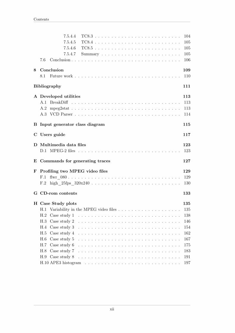
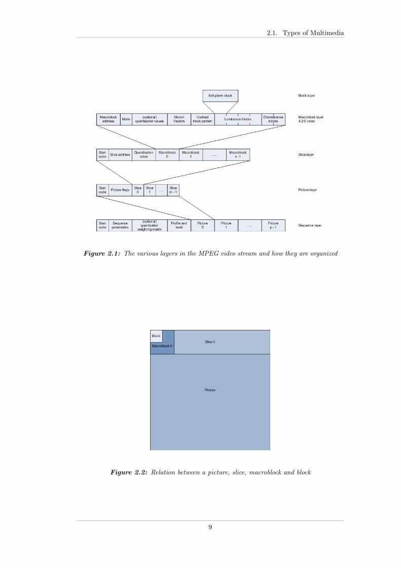
Figure 2.1 shows how the MPEG video stream is organized in the various layersaccording to the MPEG standard. Where the sequence layer contains all the pictures,and the slice layer contains a set of slices where each slice corresponds to a set ofhorizontal macroblocks. The macroblock layer contains the 8x8 pixel blocks forluminance and chrominance. The MPEG video stream in the figure uses the 4:2:0subsampling. Figure 2.2 shows how the picture, slice, macroblock and block layersare related.
The MPEG standard uses complex and computational demanding algorithms forcompressing the raw video, where the compression ratio typically is in the order of10. An example is that a video with a resolution of 720x576 and 25 fps has a rawbit rate of 166 Mbps, while the compressed MPEG will be approximate 15 Mbps[TN95]. Obviously the compression and decompression will result in a minor loss ofpicture quality, but this is often negligible.
The reduction of the bit rate can be obtained by taking advantage of the redundancyoften found in video files. There is basically two types of redundancy:
Psycho visual redundancy Details near object edges or around shot changes areless visible for the human eye, this can therefore be exploited in the reductionof the bit rate [TN95].
Spatial and temporal redundancy Most often the value of neighbouring pixelsin a frame are closely related, both within the same picture as well as acrossframes [TN95].
1Red Green Blue
8
2.1. Types of Multimedia
Figure 2.1: The various layers in the MPEG video stream and how they are organized
Figure 2.2: Relation between a picture, slice, macroblock and block
9
Chapter 2. Multimedia
In the MPEG coding algorithm the two techniques used for utilizing the redundan-cies described above are inter-frame 2-dimensional Discrete Cosine Transformation(DCT) and Motion compensation Prediction (MP).
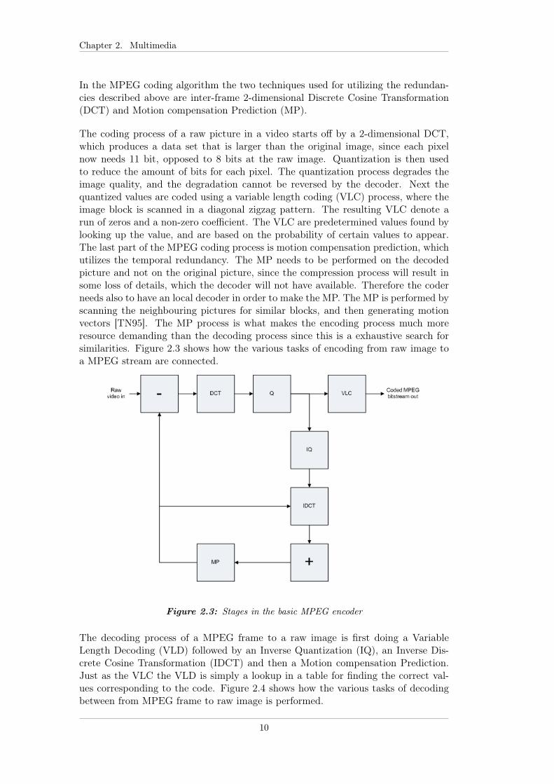
The coding process of a raw picture in a video starts off by a 2-dimensional DCT,which produces a data set that is larger than the original image, since each pixelnow needs 11 bit, opposed to 8 bits at the raw image. Quantization is then usedto reduce the amount of bits for each pixel. The quantization process degrades theimage quality, and the degradation cannot be reversed by the decoder. Next thequantized values are coded using a variable length coding (VLC) process, where theimage block is scanned in a diagonal zigzag pattern. The resulting VLC denote arun of zeros and a non-zero coefficient. The VLC are predetermined values found bylooking up the value, and are based on the probability of certain values to appear.The last part of the MPEG coding process is motion compensation prediction, whichutilizes the temporal redundancy. The MP needs to be performed on the decodedpicture and not on the original picture, since the compression process will result insome loss of details, which the decoder will not have available. Therefore the coderneeds also to have an local decoder in order to make the MP. The MP is performed byscanning the neighbouring pictures for similar blocks, and then generating motionvectors [TN95]. The MP process is what makes the encoding process much moreresource demanding than the decoding process since this is a exhaustive search forsimilarities. Figure 2.3 shows how the various tasks of encoding from raw image toa MPEG stream are connected.
Figure 2.3: Stages in the basic MPEG encoder
The decoding process of a MPEG frame to a raw image is first doing a VariableLength Decoding (VLD) followed by an Inverse Quantization (IQ), an Inverse Dis-crete Cosine Transformation (IDCT) and then a Motion compensation Prediction.Just as the VLC the VLD is simply a lookup in a table for finding the correct val-ues corresponding to the code. Figure 2.4 shows how the various tasks of decodingbetween from MPEG frame to raw image is performed.
10

2.1. Types of Multimedia
Figure 2.4: Stages in the basic MPEG decoder
The MPEG encoding and decoding processes described above are only the basic partof the MPEG standard. There are also more elaborate coding techniques which areused for enhancing the quality of the stream. These are however outside the scopeof this thesis, and the reader is referred to the official MPEG website for furtherreading [MPEGOrg]. Both the MPEG encoder and decoder are available as a simpleC implementation and can be downloaded from the MPEG homepage [MPEGOrg].It is this implementation that has been used for generating the required traces forthe DiMAS simulator.
2.1.2 MP3
The audio part of the MPEG-1 standard defines three layers of audio coding/decod-ing techniques, being MPEG layer I, II and III. The techniques rise in complexityfrom layer I to layer III, and the required bit rate for streaming audio is reduced.The MPEG layer III is typically abbreviated MP3 [RR02].
The MP3 compression algorithm utilizes a number of tricks making it possible tohave compression ratios of up to 1:12 between MP3 bit stream and Pulse CodeModulation (PCM). The human ear is not able register sounds below 20 Hz andabove 20 kHz, the top level is even reduced with the age, and most people are notable to register sounds above 16 kHz [BP00]. Therefore the audio sampling needsonly be performed within this interval. Further the human ear has 24 frequencybands, therefore masking can occur when tones within the same band are played.This can be used to reduce the bit rate, since there is no need to play the tones whichare non perceivable by the human ear.
The PCM signal is used for storing audio, and has two parameters, being samplingrate and bit rate. The sampling rate is given in Hz and and the bit rate is given asbit per second similar to the bit rate in MPEG videos. The size of the sampling ratedetermines the range of the frequencies, increasing the sampling rate will thereforepresent more tones. The bit rate determines the resolution of the sound, increasingthe bit rate will reduce the noise introduced by the MP3 coding algorithm.
The MP3 stream structure is shown in figure 2.5. A MP3 file consists of a series offrames, which each correspond to 26 ms of audio, where each frame contains 1152samples2. A frame is divided into two granules that each contain half of the samples
2Only the MPEG-1 layer 3, the layer 1 and 2 have less samples
11

Chapter 2. Multimedia
Figure 2.5: Stream structure of a MP3 file
Figure 2.6: Encoding process of a MP3 file
in a frame. For stereo audio each granule contain samples for a left and a rightchannel. The last level in the MP3 stream contains the Huffman coded bits andthe scale factors. The Huffman coded bits contain the actual data, while the scalefactors are used for reducing the quantization noise.
The MP3 encoding process is shown in figure 2.6. The filter bank samples 1152PCM signal and filters them into 32 frequency bands, that are equally spaced. Inparallel a Fast Fourier Transform module converts the PCM signals from the timedomain to the frequency domain. The psycho-acoustic module analyses the signalfrom the FFT module. Based on the human audio perception, as described earlierthe psycho-acoustic module selects a window type the MDCT should use for process-ing the incoming signals. The window type is based on the difference between thesucceeding and the proceeding frames. The quantization and scaler module is aniterative module where the sampled values are quantized and scaler values are usedfor minimizing the noise induced by the quantization. Finally the values are Huffmanencoded and the bit stream is created with side information that the decoder usesto identify the stream parameters.
Figure 2.7 shows the MP3 decoding process from MP3 bit stream to a PCM stereosignal. The decoder starts off by parsing the bit stream into header information
12

2.2. Metrics
and the actual data. The data is then decoded using the Huffman algorithm. Nextthe data is rescaled using the scaling information parsed in the bit stream, and aninverse quantization is performed. The data is split into two channels if the incomingaudio data is a stereo signal. Afterwards the IMDCT and filter bank conversion isperformed on each of the signals, which then results in the decoded PCM signals.
Figure 2.7: Decoding process of a MP3 file
The reader is referred to [RR02] for a more elaborate explanation of the MP3 encod-ing and decoding techniques.
2.2 Metrics
This section will present the general metrics that define multimedia files. Thesemetrics can be used for estimating how the quality of service for a given multimediaapplication will be. There is much literature already addressing this subject, of themost interesting are [ACH98, JN04].
The following presents the metrics that were found most relevant for describing QoSfor distributed multimedia applications. The network related parameters do not onlyapply to distributed multimedia applications, but also to locally run applications,they are however often negligible since local playback is many times faster thanplayback over a network.
Frame rate is an essential parameter for video. The frame rate needs to be suffi-ciently high in order for the video to be smooth. The frame rate is a rathersubjective value, which can vary among people. The frame rate is first of allestablished, when the encoding is performed. But some of the later parame-ters can also influence the rate while playing the video due to loss of frames.There exists standards where the frame rate is defined. The PAL format usedin Europe is 25 fps, while the NTSC format used in USA is 30 fps. Frames arealso defined for MP3 streams, here the frame rate is a static and each framecontains 26 ms of audio [RR02].
Resolution is again a very important factor for video quality, the higher the reso-lution the better quality of the video is. This is typically a static value and willnot change during playback. There could however be software that changesthe resolution, based on the performance of the network connection. Often theuser will before hand choose the resolution of the video being streamed.
13

Chapter 2. Multimedia
Sampling rate is defined for audio, and determines the span of the frequencies.More tones are available as the sampling rate is increased. The sampling rateis defined when the audio is encoded, and is typically set to 44.1 kHz, sincethis is what is used for CD audio [RR02].
Bit rate is defined for both video and audio. The bit rate is based on the frame rate,resolution and how effective the compression algorithm is. Further a video canboth be encoded using Variable Bit Rate (VBR) or Constant Bit Rate (CBR).For distributed multimedia applications it is imperative that the bandwidth ofthe network is larger than the bit rate of the file in order to ensure that framesare not lost.
Delay or response time can be interesting for distributed multimedia applications.It is however more for real-time communication like Voice of Internet Protocol(VoIP) and other phone services like Skype, Ventrilo and Teamspeak, wherethe delay must be minimal. It is crucial that the delay is low since the delayfrom one person starts talking to the other people hears him talking must below in order not to talk all at once. If the delay is more or less constant thisproblem can be overcome for ordinary multimedia applications, like video oraudio playback, by using a sufficiently large buffer.
Response time delay is similar to the delay mentioned above, but only includesthe time a stream token has spent either during transmission and the time ithas spent waiting in buffers. This is one of the metrics which are used forevaluating the performance in the case studies later in this thesis. This metricis useful due to the inter variability in multimedia, such that the performanceof two streams can be compared, regardless of the execution time needed forprocessing each of them.
Jitter is like delay a timing related parameter, which must be low for both VoIP andmore ordinary distributed multimedia applications. If the jitter is too high thequality of the sound or video may be greatly degraded due to discontinuitiesin the stream. And in worst case the application may even terminate theconnection if the jitter is too high. Again this can be overcome by usingsufficiently large buffers for ordinary multimedia applications, but it might notbe a trivial task to find this size.
Loss rate is also a central parameter that should be minimized since it greatlydegrades the quality of the stream, when packets are lost, thereby losing someof the audio or video experience. The loss of packets is most often caused bypackets not meeting the deadlines, due to congestion on the network. Loss ratecan also be seen as how many frames in a video is lost during playback.
Synchronization is also relevant for multimedia applications. For combined videoand audio applications a common synchronization is where the sound and thevideo must be synchronized correctly, this is called lip-sync. But you could alsoimagine synchronization in a distributed system, where two or more speakersneed to be synchronized in order the avoid an echo effect.
Availability is of course also an important parameter, since the media must beavailable for streaming. The media is either available or not available, so thisis not a gradient value opposed to many of the other parameters defined above.
14

2.3. Variability in multimedia
In [JN04] they propose a three layer QoS mapping, where the top layer is the Userlayer, followed by the Application layer and at the bottom the Resource layer. Theuser layer contains the subjective metrics, which are not directly measurable. Theapplication layer is said to be platform independent and contains measurable met-rics. The selected qualities selected from the user layer can be translated into someoverall metrics in the application layer. The resource layer is platform dependentand contains metrics at the hardware level. These metrics are also as the applicationlayer measurable. Figure 2.8 show how the above mentioned metrics are mappedinto this three-layer QoS model.
Figure 2.8: 3-layer model for QoS metrics
2.3 Variability in multimedia
As mentioned in the introduction, multimedia applications are examples of soft real-time tasks, which have a great variability in terms of execution time. The discussionon variability for multimedia applications is based on MPEG video since this hasbeen the main focus during this thesis.
The variability in execution time for MPEG video media sources is primarily basedon five metrics, namely frame rate, resolution, bit rate, frame type and the amountof motion. The frame rate and resolution metrics are the main contributors, andinfluences the base of execution times, while bit rate, frame type and the amount ofmotion contribute somewhat less. In general there are two types of variability, theintra variability and the inter variability.
Intra Variability is the variability within the same multimedia source. The MPEGcompression algorithm is a perfect example of this type of variability, whereexecution time depends on the type of frame that is being decoded and theamount of motion3 there is at that time.
3For MPEG video this only applies for P and B frames, not for I frames as they do not use MP
15

Chapter 2. Multimedia
Inter Variability is the variability across different multimedia sources. For theinter variability there are basically two cases. The first case is where the mediasources have the same characteristics, in terms of frame rate, resolution and bitrate, and the second where the characteristics are different. For video mediawith similar characteristics the main contributors are as in the intra variability,the frame type and the amount of motion in the video. While for video mediawith different characteristics the main contributors are resolution and framerate.
For many applications the most relevant types of variability are intra and the firsttype of inter variability. This is caused by the characteristics are often alreadypredetermined for many appliances.
The various types of variability discussed above are shown in three figures. Figure2.9 shows the intra variability in terms of execution time for a MPEG video withmotion. The top plot of the figure represents the three different types of frames inthe MPEG standard. The I-frames correspond to the value 1, P-frames correspondto 2 and the B-frames correspond to 3. It is clear from the bottom plot of figure2.9 that there is a variability in the number of instructions required for decoding aMPEG video. Further it is clear that the type of frame has a significant impact onthe variability from a intra variability point of view.
Figure 2.9: Intra variability. The top plot shows the frame type for each frame in thevideo, these are either I, P og B frames. The bottom plot show the instruction countneeded for decoding each frame.
Figure 2.10 shows the inter variability for similar MPEG videos in terms of framerate, resolution and bit rate, further the sequence of frame types is the same. Thefigure contains instruction counts per frame decoding, for four MPEG videos, wheretwo are with motion, one contains a static image and a digital watch that is countingup, and the last video is simply a static image. Again it is clear how the type of
16

2.3. Variability in multimedia
frame has an impact in terms of intra variability, but the motion in the video has aneven greater impact on the execution time in terms of inter variability.
Figure 2.10: Inter variability with similar characteristics. Number of instructionsfor four different MPEG video files. The first two data set (red and green) are MPEGvideos with motion, while the next two (blue and purple) are MPEG videos with no andminimal motion respectively.
Figure 2.11 shows the inter variability for MPEG videos with different characteristics.The characteristics that vary are bit rate, resolution and frame rate. The videos areclearly separated into three groups in terms of variability. The variability is mainlycaused by the resolution, and next the frame rate. The bit rate is the cause of thevariability within each of the three groups, and is basically and indicator of hownoisy the frames are.
2.3.1 Modelling the variability
We need a way of modelling the variability of multimedia discussed in the previoussection. The variability can be modelled using traces, these traces can either besimple ASCII files containing a list of execution times for a task or a probabilitydistribution of execution times for each task.
Retrieving the execution times from a list, is a very detailed way of simulating. Thesimulation will be performed for a very specific media file, while we often would beinterested in simulating for a broad range of media files. In order to use the simpletrace files for simulation you need to generate them, which is a time consumingprocess and the resulting trace files can be huge for long media files4. Section 6describes how the traces were generated in this thesis.
4The trace files generated for the MPEG videos, which are 15 seconds in length and have aresolution of 720x480 and 30 fps are each 30 MB in size
17

Chapter 2. Multimedia
Figure 2.11: Inter variability with different characteristics. The characteristics arebit rate (high/medium/low), fps and resolution.
The distribution describing the variability in execution times for multimedia is a niceway of providing the necessary input data for a simulation. The distributions are ofcourse based on measured execution times as the traces described above, but theyare smaller in size and can easily be altered by hand to represent a broader range ofmultimedia files. During the simulation the execution time is obtained by using thedistribution in conjunction with a random number generator.
The large variability in multimedia files is unavoidable, therefore special consider-ation must be taken, as to what the characteristics are of the target media, whenrunning the simulations. Both forms of traces discussed above can be used duringsimulation, but the distribution is the most dynamic, and can give a broader rangeof execution times. The DiMAS API does however only provide tracing functionalityusing a list of values.
2.4 Distributed Multimedia
The variability discussed in the previous section was towards multimedia run bothlocally and in a distributed manner. There is additional variability for distributedmultimedia, which is caused by the communication. The communication can both bein terms of networked applications over traditional Ethernet and in Multi ProcessorSystem-on-Chip (MPSoC) devices where the communication is performed over a bus.For distributed multimedia the variability is mainly caused by limited bandwidth,too high latency and jitter on the channel.
Ethernet is a best effort service, and it is not possible to provide any guaranties thatthe network packets will arrive at a certain time. So the arrival time of multimediabeing streamed over a network is likely to have a very high variability, depending onthe distance and the load of the channels from sender to receiver.
18

2.5. Scheduling
Modelling the variability in distributed multimedia is done in the same way as dis-cussed in section 2.3.1. Again there are the two possible ways of using traces, eithera full trace of when each packet will arrive, or using a random number generatortogether with a probability distribution.
2.5 Scheduling
Many multimedia systems have multiple tasks to perform. For example a set-top boxneeds to decode both the video and the audio of a film. At the same time it mustbe able to handle input from the user and display a Graphical User Interface (GUI)on the TV. In order to keep the expenses low, the set-top box will have a generalpurpose processor and dedicated ASICs for some of the more demanding functions.These tasks need to be performed concurrently, therefore we need a scheduler, whichcan schedule the various tasks onto the processor.
Some of the most common scheduling policies for embedded systems with hard real-time tasks are Fixed-Priority (FP) and Earliest Deadline First (EDF). These schedul-ing policies do however require that the WCET of the tasks are known. Schedulabilityanalysis techniques can then be used to guarantee that the timing constraints arerespected. As we have already seen in the previous section the execution times varya great deal depending on the multimedia file being processed, and using the WCETwill lead to over designing the system, so that it is idle most of the time.
The following sections introduce four different scheduling schemes and looks into howthey perform for multimedia applications. These schemes have all been implementedin the simulator, and will be the base of the case stories presented in section 7. FPand EDF are only lightly introduced as these are simple and well know schedulingalgorithms.
2.5.1 Fixed priority scheduling
Fixed Priority scheduling is widely used in real-time operating systems. It is one ofthe simplest scheduling techniques, where each task is given a unique priority. Thetask with the highest priority is scheduled onto the processor. FP scheduling canbe either preemptive or non-preemptive. The preemptive scheduling is based on thepriority, so a higher priority task can always preempt a lower priority task runningon the processor, and thereby gain access to the processor.
Equation 2.1 is used for making a schedulability analysis for a number of tasks beingscheduled using the FP algorithm. The symbols in the equation are given as: ci :WCET and ti : period of task i.
N∑i
citi≤ 2 · (2
1n − 1) (2.1)
This type of scheduling is probably not very suited for multimedia where tasks arecomputational heavy. Further there will always be one process which has precedenceover another, which can leave to starvation if the system is under designed.
19

Chapter 2. Multimedia
2.5.2 Earliest Deadline First
The Earliest Deadline First (EDF) scheduling algorithm is a dynamic algorithm,which also is used in embedded real-time systems. The EDF is typically used as apreemptive algorithm where the priorities are based on the deadlines of the activetasks. The task with the earliest deadline is assigned the highest priority and isscheduled onto the processor. For periodic tasks the scheduling analysis is doneusing equation 2.2, where Ci is the WCET and ti is the period of the task i.
N∑i
citi≤ 1 (2.2)
Multimedia applications are basically periodic tasks with jitter and scheduling thiskind of tasks using EDF will probably be slightly better than for FP, since the priorityof the tasks are assigned dynamically.
2.5.3 Constant bandwidth server scheduling
The Constant Bandwidth Server (CBS) is a resource reservation algorithm, whichensures that aperiodic soft real-time tasks can be scheduled together with hard real-time tasks, without jeopardizing the deadlines of the hard real-time tasks. Resourcereservation servers both exist for fixed priority and dynamic priority schedulers. TheCBS is used in conjunction with a dynamic priority scheduler as EDF.
Resource reservation algorithms are generally characterized by having a budget Q,and a period P, much like hard real-time tasks having an WCET C and a periodT. The budget specifies how much time the resource reservation server at most canassign to aperiodic tasks, within the period P. There exist both soft and hard resourcereservation techniques, [BLAC05] presents the definitions of these two types.
Definition 2.5.1. A hard reservation is an abstraction that guarantees the reservedamount of time to the served task, but allows such task to execute at most for Qi
units of time every Pi.
Definition 2.5.2. A soft reservation is a reservation guaranteeing that the taskexecutes at least for Qi time units every Pi, allowing it to execute more if there issome idle time available.
The CBS implements soft reservation, that uses tasks deadlines to optimize processorutilization, while providing temporal protection, so hard real-time tasks do not missdeadlines. The CBS controls the deadlines of soft real-time tasks, which the EDFscheduler then uses to find the next task to execute. A CBS server has a bandwidthUs = Qs
Psthat can be used for traditional scheduling analysis using equation 2.2.
When a soft real-time task goes to a running state, then it is queued into a FIFOqueue on the CBS. The tasks will be assigned a deadline if the queue is empty, orit will wait until the previous tasks have been served. The server keeps track of theserver deadline dk, which also is assigned as the deadline of the currently runningsoft real-time task.
The CBS algorithm is defined in the following
20

2.5. Scheduling
• The server bandwidth is defined as Us = Qs
Ps, which is used in scheduling
analysis.
• The server has a deadline ds, which the active CBS task is assigned.
• The server budget is decreased by the same amount of time a CBS task isrunning.
• When the server budget is depleted it is replenished, and the server deadlineis incremented as: ds = ds + Ps. The budget will never be zero for a finiteinterval in time.
• The server is said to be active if there are pending jobs.
• A job is enqueued in the server queue as it arrives at time ri. The queue isimplemented as a FIFO queue.
• If the server is idle as a job arrives, then the deadline is updated ifds ≤ ri + ( ci
Qs) ∗ Ps the new deadline is ds = ri + Ps and the budget qs is
replenished to Qs. If not then the arriving job is served with the current serverdeadline and budget.
• When a job terminates then the next in queue is served using the current serverdeadline and budget. The server becomes idle if the queue is empty.
Listing 2.1: CBS pseudo code1 When job t_j arrives at time r_j2 enqueue the request in the server queue3 n = n + 14 if(n == 1) // the server is idle5 if(r_j + (q_s / Q_s) * T_s >= d_s)6 d_s = r_j + P_s7 q_s = Q_s8 else // nothing else is done if the server is active9 When job t_j terminates
10 dequeue t_j from server queue11 n = n - 112 if(n != 0)13 serve the next job with current server deadline and budget14 When job t_j executes for a time unit15 q = q - 116 When (q == 0)17 // server bandwidth exhausted18 d_s = d_s + P_s19 q = Q_s
The purpose of the CBS is to provide temporal protection for hard real-time tasksnot to miss their deadlines, while still serving soft real-time tasks as much as pos-sible. The strength of the CBS is that it can ensure that a task is not hugging theprocessor thereby starving other tasks. This type of scheduling is specifically aimedat continuous media tasks, and will therefore probably be an effective schedulingalgorithm.
The CBS algorithm can be used in a couple of different ways for systems wheremultiple soft real-time tasks need to be scheduled onto a processor:
• One CBS can schedule all soft real-time tasks
21

Chapter 2. Multimedia
• One CBS for each soft real-time task can be used
If the first approach is used then the scheduling will more or less be done as plainFP scheduling for the soft real-time tasks, since the CBS unit provides a dynamicdeadline for the first task in the queue. Only when the first task in the queueterminates, will the next task in the queue gain access to the processor.
The second approach is much more suited for soft real-time tasks, since this providesa degree of fairness, where all tasks are given processor time. The scheduling willprobably look much like a time division multiple access algorithm, since the serverbandwidth basically corresponds to a time quantum.
For more details on the CBS the reader is referred to the Soft Real-Time systemsbook [BLAC05].
2.5.4 Linux scheduler
Two different scheduling algorithms are used in the Linux 2.6 kernel. In this thesiswe will look at the scheduling algorithm used in the kernels up to 2.6.23, since this iswhat the Windriver linux 5 kernel uses. The scheduler used in the 2.6.23 and upwardsis the Completely Fair Scheduler (CFS), more information can be found at [MH07].For the remainder of this section the 2.6 kernel will refer to kernels below 2.6.23. Thescheduler for this kernel is is named O(1), since it runs in constant time regardlessof the number of tasks.
The Linux kernel 2.6 works with two classes of tasks, real-time tasks and normaltasks. Every task is given a priority, in the range of 0 to 140, where 0 to 99 areassigned to real-time tasks, while 100 to 140 (the nice range) are assigned to normaltasks. The scheduler uses a preemptive, priority based time-sharing algorithm. Thetasks are assigned time quanta according to their priority, the high priority taskshave the largest time slice [SGG09].
The scheduler works with two queues, one for tasks which are runnable and one fortasks that have spent their time quantum. Normal tasks are only considered runnablein the case that they have not already spent their time slice, whereas real-time tasksare runnable until they are done. When all the tasks in the runnable queue havebeen moved to the expired queue the counters are reset and execution starts over. Atthe reset the priorities are further dynamically incremented or decremented with amaximum value of 5, depending on how much time each task has spent sleeping. Thisis however not performed for the real-time tasks [SGG09]. The reason for assigningtasks with high idle time higher priorities is that they often are interactive tasks, andthey should therefore have a high priority, so the user has a good experience usingthe system.
The real-time tasks are not influenced by the time sharing and will run to completionbefore any of the normal tasks will have a chance to acquire the processor. The real-time tasks are scheduled with preemptive fixed-priority, where the highest priority
5The Windriver linux is widely used in embedded systems.
22

2.5. Scheduling
Figure 2.12: Linux scheduling queue for active and expired tasks within the sameepoch. The scheduler in this example is assigned 4 real-time tasks and 9 non real-timetasks.
task is scheduled onto the processor. For real-time tasks with the same priority, thescheduling is performed either using a First-Come-First-Served (FCFS) or a Round-Robin (RR) algorithm. FCFS is a FIFO style algorithm, were the active task keepsthe processor until it is done. RR is a time sharing algorithm, where each task isassigned a time quantum, and when it is expired, the task is put at the end for thequeue and the time quantum is replenished. Real-time tasks are only moved fromthe active queue to the expired queue once they have completed [SGG09].
Multimedia applications are defined as soft real-time tasks and can therefore beassigned as real-time tasks in the Linux operating system and have the highest pri-orities. Assuming the system is not under designed, then the large variability in themultimedia tasks will make it possible for the normal tasks also getting some proces-sor time. The multimedia tasks are however probably the most processing intensivetasks in the system, while some of the normal tasks might be shorter. With theLinux scheduling the short normal task will have to wait for the long real-time tasksto finish, before it can be scheduled.
Next there is the FCFS and RR scheduling algorithms which are used for real-time tasks that have the same priority. Both algorithms serve the task, which hasbeen waiting the longest time in the queue. This kind of scheduling seems to be agood choice for soft real-time tasks like multimedia, since some deadline misses areacceptable.
2.5.5 Hypothesis
The Fixed-Priority and the Earliest Deadline First scheduling algorithms are bothhard real-time scheduling algorithms, and are not well suited for soft real-time sys-tems where the resources are scarce. The FP is probably the worst, since systemswith limited resources can end with starvation of the lower priority tasks.
Scheduling using the Linux O(1) scheduler will be similar to the FP scheduler formultimedia tasks that are scheduled as real-time tasks. As already mentioned thiscan lead to very poor performance for other applications that for example providea user interface. Therefore it is more interesting to look at how the multimediaperforms when assigned as user tasks, and have a lower priority than the user in-terface application. This makes sense under the assumption that the user interfaceapplication is only seldom active.
23

Chapter 2. Multimedia
The Constant Bandwidth Sever is a resource reservation service, which ensures thathard real-time tasks can operate on the same processor as soft real-time tasks, whilenot jeopardizing the deadlines of the hard real-time tasks. The CBS is however nota scheduling algorithm in itself, the CBS works on top of another deadline orientedscheduler like EDF. Having one or more CBSs controlling the deadlines of soft real-time tasks on a processor, where no hard real-time tasks are running, might not turnout to be much different from an ordinary EDF. It should however ensure that onlythe tasks which have very high variability suffer for this, while the rest are unaffected.
24

Chapter 3
Simulators
Figure 3.1: Classification of simulators
Generally simulators can be classified into two groups, one being architectural andanother being micro-architectural, these are respectively concerned with functionaland performance simulation. A micro-architectural simulator is more or less a soft-ware implementation of a microprocessor with instruction set, cache and pipelineemulation.
The micro-architectural simulators can further be classified into scheduler and cycletime simulators. The scheduler simulators are the simplest of the two, in the sensethat the instructions are executed in-order according to resource availability. Thistype is called an Instruction Set Simulator (ISS). The cycle time simulators are cycleaccurate and emulates the processor into details with cache hits and misses andpipeline stages. This type of simulator is also called a Cycle Accurate Simulator(CAS).
In addition to the ISS and CAS we also have Full System Simulators (FSS), the threetypes are elaborated below [MY07, ALE02]:
ISS An Instruction Set Simulator (ISS) is a simulator which emulates a processorat the micro architectural level. An application is run on the simulator where
25

Chapter 3. Simulators
each instruction is executed in-order and the simulator can thereby simulatethe functionality of the applications. This leads to fairly accurate simulations,but performance measurements are however not that reliable.
CAS A cycle-accurate simulator is a software implementation of a hardware device,typically a processor. Here cache hit and misses, branch predictions and theflow of every instruction through the various pipeline stages is simulated. Acycle-accurate simulator basically simulates all the internal states of the micro-architecture. Therefore it is even able to simulate out-of-order instructions,where instructions can be delayed for several machine cycles for example dueto floating point operations. This kind of simulator is able to make very detailedperformance measurements of the processor, but it has a cost in terms of thetime required for running simulations.
FSS Full System Simulators typically include an ISS or preferably a CAS, and com-bines it with peripheral entities like memory and disc I/O. Typically a FSS isbuilt as a virtual machine, which makes it possible also to run the applicationson top of a real operating system. Obviously a FSS is a very resource demand-ing simulator, and it is able to present very detailed performance metrics.
As seen in figure 3.1 the architectural simulators can also be classified into variousgroups and subgroups. At the first level we have trace driven opposed to the ex-ecution driven simulators. The trace driven simulators uses traces recorded fromprevious program execution for measuring performance of an application. This wayall functionality of the application has been saved and the simulator need not worryabout the functional execution or the I/O devices. Therefore similar simulations us-ing a trace driven simulator will always end up with the same performance measure-ments. The execution driven simulation is more complex than the trace driven sincethe functionality of the application is simulated as it is executed. Further the simu-lator needs to supply the various I/O devices that the simulated application mightneed. Specially execution driven simulators using networked devices can have vary-ing performance measurements, since the performance of the network can vary fromsimulation to simulation. This variation can however be dealt with using traces forthe I/O devices while running the execution driven simulation [ALE02, SSTutorV4].
Finally an execution driven simulator can either be performed using emulation ordirect execution. Simulators which use emulation for simulating an application typ-ically requires some kind of ISS. While a direct execution simulator utilizes the hostarchitecture for executing the application, this is often referred to as co-simulation.Obviously direct execution requires that the host architecture is similar to the targetarchitecture of the application which is simulated [MY07].
3.1 Levels of Abstraction
As seen in the previous section simulators vary a great deal in levels of abstraction.The abstraction pyramid in figure 3.2 shows the connection between accuracy, costand abstraction of a model. The accuracy and cost of the simulation is low at the highabstraction levels, while it is high at the low levels of abstraction. Accuracy is meant
26

3.2. Design-Level Simulator
as the level of details in the model which is simulated, meaning how accurate themodel is compared to the architecture. Cost covers how much resources are neededfor the simulation both in terms of the simulation time and amount of memory usage.Further the abstraction pyramid shows how the design space for very abstract modelsis large, whereas the design space is narrowed as the abstraction of the model islowered [ZL02].
Figure 3.2: The Abstraction Pyramid [ZL02]
The micro-architectural simulators which were mentioned in the previous section areat the low level of abstraction and therefore reside in the area around approximatemodels and cycle-accurate models. The architectural simulators are at a somewhatmore abstract level and reside around executable behavioural models and approximatemodels. As we will see in section 3.2 the architectural simulators can also reside atthe top level of the abstraction pyramid namely back-of-the-envelope.
For prototyping it is preferable to have a model of high abstraction, since the modelmust be fairly simple and quick to create, further the simulation must be done withina reasonable time. Once the target architecture and the application code is written itis interesting to have a more detailed model, which can be used for extracting variousforms of performance metrics like WCET, power consumption or code verification.
3.2 Design-Level Simulator
The previous section presented the various forms of simulators shown in figure 3.1and the abstraction pyramid in figure 3.2. However there is still one missing piecenamely the top level of the abstraction pyramid the back-of-the-envelope model. Thiskind of simulator is an architectural model, but does not use executable code for thetarget architecture during simulation. Instead the emulator can be seen as a highlevel description of how the architecture works and the user application as code
27

Chapter 3. Simulators
describing what needs to be done. This type of simulation is referred to as Design-Level Simulation.
As mentioned in section 3.1 the resulting design space for models of high levels ofabstraction is large, this is what is needed at the design-level simulation. Since thesimulations are merely conceptual to see how it would be possible to construct agiven system. Later on in the design and implementation process it will be inter-esting to create more accurate models, in order to get more reliable performancemeasurements.
The DiMAS API that is developed in this thesis is used for creating design-levelsimulators, which are trace driven. The traces are used both for generating tokensfrom input devices, while other traces are used for reading the execution times foreach request.
3.3 Existing Simulators
This section will present some of the existing simulators, which are able to simulateboth at the architectural and the micro architectures level. These simulators arewell known and are used both commercially and academically. Likewise some arecommercial while others are open source projects. Many of the simulators can beconfigured to simulate applications at various levels of abstraction, and thus notbound to one area of the abstraction pyramid in figure 3.2.
3.3.1 SimpleScalar
SimpleScalar from SimpleScalar LLC is an open source project, which dates back to1994 and is still under development. The simulator is highly used in the academicworld and is often used in research papers for performance evaluation.
The SimpleScalar is a complete tool set with a series of different simulators whichvary in the level of details. The simulators range from very simple ISS, which onlyemulates the instructions to simulators which take cache hit and misses, pipelinestages and even branch prediction into account. Figure 3.3 summarizes the varioussimulators which are part of the SimpleScalar tool chain.
Only the sim-outorder simulator is a CAS, which therefore can simulate a processorwith relative high accuracy. The simulation is however very time consuming and asimulation, which takes a couple of hours using a simpler simulator like sim-profilecan take a day with the sim-outorder simulator.
As part of the tool chain is a simple text driven debugger dlite!. Only the sim-safesimulator is not able to use the debugger. Simulation is done interactively whenusing the debugger, where the user can specify breakpoints for either instructions orfor global variables. The simulation is then performed either by stepping over eachinstruction or by running until a breakpoint is hit.
28

3.3. Existing Simulators
Figure 3.3: The Various Simulators within the SimpleScalar Tool chain [SSTutorV4]
The simulator source code is very modular and can therefore easily be customized tosupport specific features like tracing. During the work on this thesis the debugger wasextended to implement a tracing feature based on breakpoints, section 6 elaborateshow this extension is implemented.
The reader is referred to [SShome, SSTutorV4] for more details on the SimpleScalartool chain.
3.3.2 Simics
Simics from Virtutech is a commercial simulator, which supports PowerPC, x86,ARM and MIPS architectures. The Simics simulator is a FSS, which emulates achosen hardware device, both with the processor as well as various types of I/Odevices. Basically the simulator is a virtual machine. The virtualization makes itpossible to execute the same binaries in the simulator as on the physical hardware.A further advantage of the virtualization is that the simulation can be run with anoperating system and multiple applications [SimicsDS].
Simics is an execution-driven simulator that even is able to emulate multi core pro-cessors and other types of System on Chip (SoC) hardware. The simulator is de-terministic in the sense that the same execution can be performed multiple timeswith the same timing parameters, thereby making it easier to debug timing relatedbugs. When using breakpoints during simulation the whole system is halted, in-cluding timers and interrupts. The user is then able to extract debug informationof the system, and continue the simulation without the simulated applications andoperating system noticing the delay [SimicsWP].
Simics can capture detailed information regarding the target hardware architecturefor making cache analysis or general performance analysis. It is also possible toperform network simulations using Simics.
29

Chapter 3. Simulators
3.3.3 PTLsim
PTLsim is a cycle accurate simulator, the PTLsim/X is an extension making it afull system simulator, which incorporates a virtual machine environment like Simics.The details of the simulator range from Register Transfer Level (RTL) up to fullspeed execution on the host architecture, which is done through co-simulation. Agreat advantage of PTLsim over Simics is that the simulator source code is publiclyavailable, and can therefore be altered to suit the users needs.
The PTLsim simulator is restricted to 32/64-bit x86 Instruction Set Architectures,but with PTLsim/X the simulator can simulate 64-bit multiprocessor architectureswith up to 32 processors [MY07].
3.3.4 SystemC
SystemC is an API for C++ which features classes that can be used for modellingboth software and hardware. It can therefore also be used for modelling systems asa combination of software and hardware. SystemC is capable of modelling systemsat multiple abstraction levels and can even model complete systems, where variouscomponents within the same system are modelled at different levels of abstraction.
Figure 3.4 show various modelling languages and what they can model ranging fromtransistor level to system requirements. SystemC is both capable of modelling as lowas the Register Transfer Level (RTL) like VHDL and Verilog and through functionaland up to architectural level. This makes SystemC a very attractive language, andseeing that the language simply is a set of C++ classes most C++ programmers willbe able to learn the language fairly easily.
Figure 3.4: Comparison of SystemC and other design languages [BD04]
SystemC includes a simulation engine, which is capable of running a simulation of themodel. The engine is able to simulate timing constraints if the various modules in themodel are augmented. A specialized class sc_time is used for representing time in
30

3.3. Existing Simulators
the models. Logic in the modules are performed in zero time1, unless augmentation isinserted to give a notion of time. The engine can use delta cycles2 in the case, wheremodules are performing logic operations within the same time window. This can beused by the user for making sure that the simulation of the model is deterministic.
Since SystemC is written in C++ it is possible to incorporate application code writ-ten in C/C++ into the simulator and run it as part of the simulation. This makesit a very flexible tool for implementing simulators.
SystemC is however simply an API, so building a simulator requires some moreelaborate programming compared to some of the other simulators presented in thissection.
The basic idea of SystemC is to create various modules, the modules communicateusing channels which typically are signals or FIFO buffers. Customized channels canalso be created, where specific behaviour is required. This could for example be aspecific communication bus, like the CAN bus. The modules can have a notion oftime, which can be implemented either as a global clock signal or simply using waitstatements.
There are many books about SystemC and how it can be used for creating simulators,for more elaborate description of SystemC the reader is referred to [BD04, GLMS02].
3.3.5 Pesimdes
Pesimdes is a simulation library, which is an extension of SystemC. Pesimdes is de-signed for creating simulators that can simulate distributed hard real-time embeddedsystems. The maximum backlog3 in buffers is analysed after a simulation and usedfor evaluating if deadlines were missed. Further the response time4 for task communi-cation can be analysed. Multiple tasks can be mapped onto one processing element,and the user can choose which scheduling policy the processing element should use.
Pesimdes does not use an ISS as part of the simulation, but uses WCET, whichtypically is obtained using static analysis techniques with programs like aiT fromAbsInt. The simulation is therefore performed at a higher level of abstraction, andno functional user code is required for the simulation.
Pesimdes is implemented in SystemC and will be the base of implementation for thesimulator in this thesis. Section 4.3 will elaborate further on specific details of thesimulator.
3.3.6 ARTS
ARTS is a system level simulation framework, which has been developed at theTechnical University of Denmark (DTU). The framework is implemented in SystemC
1No time is passed in the simulation environment. This is not the actual time it takes to performa simulation.
2There can be multiple delta cycles within the same simulation time window.3Backlog defines how much space is occupied in a buffer4Time from the token is generated until it arrives at the final destination
31

Chapter 3. Simulators
and is used for both modelling and simulation of Multi Processor System-on-Chip(MPSoC). The framework makes it possible to analyse different layers and theirinteraction in a system. This could for example be the application, middleware andarchitectural layer.
The framework uses a set of input files containing the application models and theplatform models, which are expressed in the ARTS scripting language. The appli-cation model file describe the various tasks in each application and how they areconnected using task graphs. The platform model file describes processing elementsand network components. For simulation another file is used for making the mappingbetween applications and platform.
ARTS is very complex and is capable of collecting a large amount of statistics,examples of these are peak memory usage, average and maximum utilization ofprocessing elements and deadline misses. For a more in-depth explanation of ARTSthe reader is referred to [MVM07].
3.3.7 Summary
The six simulators presented in this chapter, range from cycle accurate simulators tosystem-level simulators, equivalent to the bottom and top of the abstraction pyramid,seen in figure 3.2. The simulators have been summarized in table 3.1, where the twomain categories micro-architectural and architectural from the classification tree infigure 3.1 are included. The table has been divided into two parts, a lower partwith simulators for doing performance analysis at a low level of abstraction, and theupper part for system-level simulators, which are located in the top of the abstractionpyramid.
The SystemC simulator is a special case, in the sense that it is not a pre-built simu-lator, but rather an API for modelling both hardware and software. But SystemC istypically used for modelling systems at the architectural level, and often as system-level simulators, therefore it has been included in the upper part of the table. ButSystemC could just as well be implemented using an instruction set simulator, oreven modelling a microprocessor at the register transfer level.
Name Micro- Architectural Type LicenseArchitectural
Pesimdes No Yes System-level Open SourceSystemC (Yes) (Yes) All Open SourceARTS No Yes System-level Open Source
SimpleScalar Yes Yes ISS/CAS Open SourceSimics Yes Yes ISS/CAS/FSS CommercialPTLsim Yes Yes ISS/CAS/FSS Open Source
Table 3.1: Short summary of the simulators from this chapter
Pesimdes was chosen to be the base of the DiMAS simulation API, due to the modularand simplistic design. Pesimdes can therefore easily be extended to support soft real-time tasks, instead of only supporting hard real-time tasks.
32

Chapter 4
Design of the Simulator
This chapter presents the design of the DiMAS simulation API. The first sectionpresents a overview of what should be simulated. Next the requirements for the sim-ulator are presented in section 4.2. Section 4.3 elaborates on the design of Pesimdes,while section 4.4 contains the actual design of the DiMAS API, where the main focusis on the scheduling techniques.
4.1 What needs to be simulated
It was made clear in chapter 2 that multimedia is highly variable in terms of executiontimes. Multimedia is a continuous media, which due to its variability is characterizedas aperiodic. The purpose of the simulator is to simulate multimedia and otherminor tasks for example user interface applications, which are highly aperiodic. Thesimulator therefore needs to simulate aperiodic tasks, which vary in execution times.
The multimedia that needs to be simulated is both video, audio and other generalapplications. Basically the simulator must be able to simulate both soft and nonreal-time tasks. It might however be valuable if hard real-time tasks also can be apart of the simulation.
A key objective for the simulator is the ability to simulate distributed multimediaapplications. Therefore the simulator must be able to model a system with multipleprocessing elements and multiple tasks running on each processing element. Furtherit must be possible to model the variability on the input side for example from anetwork connection, where jitter and burst of data can occur.
The purpose is to create a model of a given multimedia system, and check howpowerful the processing elements needs to be in order for the system to obtain asufficient QoS. Task mappings, processor scheduling algorithms, processor speedsand buffer sizes can be customized in order to obtain the best result.
The end result is a system-level simulator, that presents a good estimate of how wellthe system will perform. The performance details are narrowed into only the most
33

Chapter 4. Design of the Simulator
vital metrics, and the input data can be qualified guesses of the resource require-ments for the various tasks. This high abstraction level is desired both in order forsimulation speeds to be kept low, but also due to the high variability in the multi-media. The high variability is the source of why the simulation must be done at ahigh level of abstraction, since lowering the abstraction level only will result in moredetail performance estimates for a specific set-up with a specific set of input.
The metrics that are used for evaluating the QoS for a system model are given inthe following.
Lost frames This is probably the most obvious metric of them all. Frame lossboth for video and audio is a central part of the QoS metrics. It is crucialthat the loss of frames is kept at a minimum, in order to deliver a good userexperience. Recall that this metric is at the user layer in the three-layer QoSmodel presented in section 2.2.
Response time is a measure of how much time the token has spent waiting from itwas generated until it arrived at the output. The response time is a very goodmeasure for comparing the schedulers on similar set-ups, where parametershave been customized.
Buffer backlog is the third metric, and it gives an idea of whether there are anyserious bottlenecks in the model. If this is the case, then the parameters needto be changed in order to have a satisfactory system.
4.2 Requirements
A fully functional simulator requires a number of different modules, namely inputdevices, processing elements, tasks and output devices. All but the processing ele-ment modules need a notion of time in order to function during a simulation. Thisnotion is given as input data and summarized in the following.
Input rate determines how often a token should be generated in the test bench.For MPEG video files, a token corresponds to a macroblock. The input rate isrelated to the input devices for a simulation test bench.
Consumption rate is similar to the input rate, but this is however the rate at whichthe tokens should be consumed at the output end of the test bench. This ratecan however in some situation be unnecessary if there are not constraints as tothe consumption.
Execution times is a central parameter for this simulator, since the focus is onscheduling techniques and how they perform. The execution time can both bespecified in time units or in cycle counts, the latter requires a processor speedfor the processing element.
The input rate can both be strictly periodic, periodic with jitter, or aperiodic usingtraces from a text file. It is assumed that the consumption is constant both in terms
34

4.3. PESIMDES
of period and amount. Further if there is no interest in comparing the performanceof the system relative to a specific consumption, then this part can be disregarded.
The various tasks that are running in the system must be assigned an executiontime. This can either be a static execution time as in hard real-time systems, wherethe WCET typically is used, or it might be some kind of trace. When running asimulation care must be taken as to the timing specified in all three types of inputin order to avoid either buffer over- or underflow.
Processing elements are in this simulator referred to as resources. All resources ina simulator test bench are associated with a scheduling technique of some kind.The scheduling techniques that are part of the DiMAS framework have already beenintroduced section 2.5, being Fixed-Priority, Earliest Deadline First, Linux O(1) andConstant Bandwidth Scheduler.
The output files which the simulator can generate are buffer backlog for specificbuffers in the system, response time for the various input tokens and logging oflost frames. Performance analysis of the simulated set-up can then be based onthese three output, where graphs can be generated, but the minimum, average andmaximum values are also useful for a quick overview of the performance.
The DiMAS simulator is basically an extension to the Pesimdes simulation API, andis like wise an API. Therefore a simulation requires a test bench, which is createdusing the various modules supplied in the API, and a C++ compiler is used in orderto create the final simulator.
4.3 PESIMDES
PErformace SIMulator for Distributed Embedded Systems is a simulator written bySimon Perathoner in 2006 at the Swiss Federal Institute of Technology. The simulatoris able to simulate hard real-time distributed embedded systems, and can be usedfor analysing the maximum backlog in buffers and the response times for tokens sentthrough the system. The Pesimdes simulator is basically an API, and the user usesvarious components to construct a test bench. The API is based on the SystemClibrary, which was introduced in section 3.3.4. Therefore the simulator requires thatthe SystemC library has been compiled successfully. The SystemC library is thenlinked into the users simulator at compile time. The basic components of Pesimdesare described below.
Input stream generators The purpose of these modules are to generate tokens,which simulate communication between two tasks. Pesimdes include four typesof input generators, these are periodic, periodic with jitter, periodic burst withjitter, and using a trace file. All generators generate a token with a time stamp.
Resources These are the actual processing elements. The resources have embeddeda scheduler, which either can be, Fixed-Priority (FP), Earliest Deadline First(EDF), or Time Division Multiple Access (TDMA), which are typical hard real-time scheduling algorithms. The scheduling algorithms are both implementedas preemptive and non-preemptive.
35

Chapter 4. Design of the Simulator
Tasks can be run on a resource, and are mapped onto this resource at compile time.A task is only assigned to one resource. The tasks can have multiple inputdependencies and can send multiple tokens each time they are executed.
Buffers An extension to the standard sc_fifo channel has been implemented inorder to register the maximum backlog that was registered in the buffer.
Display A class which consumes the tokens and is used for calculating the responsetimes of the tokens, that is the time from the token was generated until it wasconsumed by the output_display object.
A test bench is constructed in a C++ file, where the Pesimdes header file is included.A tasks object needs be be created for each task in the system. Further the variousresources are initialized, where the number of tasks each resource needs to serve ispart of the parameters. WCET, period, deadline and priority of a task is assignedwhen the tasks is mapped onto a resource. The parameters depend on which typeof scheduling algorithm a resource use, for example the FP needs WCET, periodand priority, while the EDF needs WCET and dead line. The communication be-tween tasks are performed using FIFO buffers, which have been extended to createstatistical information as mentioned earlier.
Pesimdes is an API for creating system-level simulators, where no functional codeis needed. The resulting simulators can be used for analysing the memory andtiming requirements of a distributed system. The tokens that the tasks in the systemcommunicate with use a data structure for storing the generation time of a token,and the last time a token was processed. These data are used for the timing analysisand for the EDF scheduler.
For further details on the Pesimdes API the reader is referred to the master thesis[SP06] by Simon Perathoner.
The previous sections have already discussed what the purpose of the DiMAS simu-lator is, and specifically what the requirements are, the next section will clarify whatadditional functionality is added and outlines how this is designed.
4.4 Structure of the simulator
The general modules, which are part of the DiMAS simulator API are show in figure4.1. The modules which are encapsulated in a green box are modules from thePesimdes API, which have been altered in the DiMAS API. The modules, which areencapsulated in a red box are new modules, which were implemented for the DiMASAPI.
The Resources in figure 4.1 correspond to processing elements with different schedul-ing techniques. All resources can be assigned a finite number of tasks which theyneed to schedule according to their scheduling algorithm. The whole resource grouphas also been encapsulated in a red box, since all of the resources inherit from a
36

4.4. Structure of the simulator
new abstract class, which has tracing functionality. The design of each resource iselaborated further in section 4.4.1.
The input stream devices include periodic, periodic with jitter, periodic with burstand input from a trace file. These are the same input types that are used in thepesimdes simulation API and no additional input devices are required for the DiMASAPI.
The output devices are generally devices which consume tokens, and record statisticalinformation from a simulation, which can be logged to output files. The Displayand Display and write modules calculate the response time information for eachtoken, further the display and write module writes the tokens to a buffer for furtherprocessing. The Consumer module is a module, which consumes a given amount oftokens at a given rate. The module logs an error if the input buffer did not containsufficient tokens, and then flushes the buffer.
The various group contains modules which have no other related modules, but arejust as important. The Pesimdes simulation API introduced an extension to thestandard FIFO buffers in SystemC. These buffers record the maximum backlog thebuffer has experienced. These buffers are further extended in the DiMAS API withthe ability to trace the backlog into a trace file. A crucial part of the API is thetask module, which corresponds to a single task. The task module can have multipleinputs and outputs for communicating. The Time status module is module thatcan be used for printing the simulation time progress to standard output duringsimulation. This is useful when running long simulations, where no other output ispresented. The last module in the various group is the Constant Bandwidth Serverwhich is a module that can be used in unison with the EDF scheduler to scheduleboth hard and soft real-time tasks on the same processing element. The CBS hasnot been included in the resources group since it is not a scheduler in it self. TheCBS module is designed such that it also can be used with other deadline orientedscheduling techniques.
The simulators which are created using the DiMAS API are very modular, and asseen in the previous consist of only a few different types of modules. The general ideais that each task is mapped onto a single resource, and buffers are used in betweentasks to model the communication flow. Figure 4.2 shows the general idea of howa test bench can be constructed with multiple tasks mapped onto a resource, andwhere buffers are put in between the communicating tasks. Further one of the tasksin the test bench requires two inputs before this task is ready for execution.
The communication between input, task and output devices is done using the sametoken structure as in Pesimdes, this token contains a sequence number, ID for whichinput generated it, time of generation and the time of when it last was processed.Specifically the generation time, and last processed time in the tokens are used bythe various output devices to generate the statistical information.
4.4.1 Scheduling
This section continues the discussion in section 2.5, and describes how the schedulingalgorithms are designed. The resources are similarly structured, but with some vari-ations which are required for their specific functionality. The following describes the
37

Chapter 4. Design of the Simulator
Figure 4.1: The general modules which are part of the DiMAS API. The moduleswhich are encapsulated in a green box are classes from the Pesimdes library, which havebeen altered in the DiMAS library. The modules that are encapsulated in a red box arenew classes in the DiMAS library.
Figure 4.2: Example of connections between the various modules in the DiMAS API.
38

4.4. Structure of the simulator
Figure 4.3: Resources contain one thread for the scheduler and one thread for eachtask. Each task thread is connected to the corresponding task module.
basic design, which is the same for all resources, and each subsection will elaborateon how each of the scheduling algorithms are structured.
All resources relies on a set of threads, one thread for the scheduling algorithm andone thread for each of the tasks that are assigned to the resource. The task threadsare connected with the task modules as shown in figure 4.3, where each task threadhas both an input and an output. When a task module detects a token on the inputport, a request is sent to the task thread, which then signals the scheduler. This ishowever only performed if the task thread is idle. If the task is active the task modulewill wait until the task thread is done before signalling the new request. The taskmodules and task threads communicate using channels, where the token structure issent back and forth, while the task threads and scheduler thread communicate usingsignalling in terms of global variables.
The design of the EDF and the FP resources have not changed significantly in termsof the scheduling algorithm. There is however a need for modelling the variabilityin execution time, and therefore the assignment of execution time for each task hasbeen extended so that it can be based on an input trace file as well as a constantvalue.
4.4.1.1 Fixed priority scheduling
The scheduler uses a global list containing the remaining execution times for all thetasks assigned the resource, and selects the next task to be run by looping throughthe list in priority order and selecting the first task that has not finished execution.The task is signalled to start, and the scheduler will wait for a new event from thetasks. This event is either due to the running task finishing the execution, or anothertask trying to pre-empt the running task, due to it getting a new request from thetask module. The task threads are each responsible for updating the remainingexecution time in the list before the scheduler is activated. The design of the FPscheduler has not changed significantly from Pesimdes.
39

Chapter 4. Design of the Simulator
4.4.1.2 Earliest Deadline First scheduling
Similarly to the FP scheduler there is also a list containing the remaining executiontime for each task assigned the resource. An additional list is used for the EDFscheduler, which contains the relative deadlines of each task. Every time the sched-uler is woken up, either by the running task completing, or another task receiving arequest, the scheduler starts by updating the relative deadlines for each task. Thetask with the smallest relative deadline is then signalled to run by the scheduler.
The EDF scheduling algorithm is typically used for hard real-time applications,where deadline misses are not tolerated. The DiMAS simulation API is howeveralso concerned with simulating soft real-time applications where deadline misses areacceptable. Therefore all tasks assigned to an EDF resource must specify if it is ahard or soft real-time task. For hard real-time tasks the simulation will terminate ifdeadlines are missed, while for soft real-time tasks the deadline will be set to zero,and simulation will continue.
4.4.1.3 Constant bandwidth server scheduling
The CBS requires a EDF scheduler to do the actual scheduling. A processing elementcan have some tasks which are scheduled only using the EDF, but also some taskswhich are scheduled by a CBS. Often there will be multiple CBSs, which have oneor more tasks assigned. The basic idea is that each time the EDF scheduler needs toupdate the relative deadlines for the tasks, the CBS is used for assigning the deadlinesof each task that is assigned the CBS. Figure 4.4 shows how the EDF scheduler can becombined with CBSs for scheduling four tasks. The figure is slightly misleading sinceit does not show that the task threads and the scheduler thread also communicateas is the case.
The EDF scheduling resource is modified in such a way that it can communicatewith one or more CBS modules, thereby realizing the CBS scheduling algorithm.
The only addition to the scheduler thread is that the CBS modules must all updatethe relative deadlines for the tasks that they are assigned to, when the EDF sched-uler updates the relative deadlines of ordinary tasks. The modifications in the taskthreads are some what more elaborate. Each time a request from the task module isreceived, the task thread adds a request to the CBS queue if the task is a CBS task.Every time the task thread receives a notification from the scheduler thread to startexecution the task thread notifies the correct CBS that execution has started. Andonce the task execution is halted, the task thread notifies the CBS of this. Once atask is terminated the task thread removes the task from the CBS queue.
The CBS modules contain a list containing tokens that corresponds to task request.This list is utilized as a First Come First Served (FCFS) list, where a task tokenis not removed from the list until it has terminated its execution. The CBS threadwaits for a task thread to signal that it has begone execution. Once started the CBSserver waits either for the task thread to notify that the task has stopped executionor until the server bandwidth has exhausted. If the bandwidth was exhausted, theCBS notifies both the running task and the scheduler thread and updates the CBSdeadline accordingly. The CBS thread now waits for a notification from one of theassigned tasks, that it is starting execution.
40

4.4. Structure of the simulator
Figure 4.4: Example of a processing element with two CBSs and four tasks.
4.4.1.4 Linux scheduler
Only the non real-time scheduling part of the Linux O(1) scheduler is part of theDiMAS simulation API. The scheduler uses a time sharing algorithm, where the sizeof the time slots vary depending on priorities. The scheduler uses two queues forseparating tasks depending on whether they have spent their assigned time quantumor not. These queues are called active and expired.
A structure for containing the ID, and the remaining time quantum for a task is usedas member in the active and expired queues. It is these tokens that the scheduleruses every time it is activated. Each of the two queues are structured as an array ofqueues, since each part of the array characterizes the priority that all tasks at thatindex has. This structure is what is shown in figure 2.12 on page 23.
The tasks with the highest priority in the active queue is always scheduled ontothe processing element, and scheduler removes the task token from the active queuetemporarily. The running task is pre-empted either if the time quantum is expired,if the task terminates or if another task receives a request from the task module. Ifthe time quantum of the running task has depleted, the remaining time quantum isupdated and the task token is put in the expired queue. If the time quantum is notspent the remaining time quantum is updated and the token in reinserted into theactive queue. If the active task terminates, the scheduler signals the task with thehighest priority in the active queue. Once the active queue contains no more tasktokens, the active and the expired queues are switched.
In this resource the scheduler thread does not know the remaining execution timesfor the tasks, only the individual task threads knows this. Once a task terminatesa global variable is set by the task and the scheduler is notified. The task threadsinsert the task token into the active queue every time there is a request from the taskmodule. The task thread will only receive a new task request from the task modulesif the task thread is idle, which is similar to the FP and EDF algorithms.
41

Chapter 4. Design of the Simulator
4.4.2 Input and output
This section will present details on the information contained in the input and outputfiles and how these files are to be structured.
All input and output files are simple text based ASCII files. The files follow theusual rule, that lines beginning with a # are assumed to be comments and will notbe read. The # must however be put as the first character in the line.
As stated in section 4.2 the simulation API can use input trace files for token gen-eration and for retrieving the execution time of a task. The trace files are of courseonly interesting when variability needs to be modelled. The token generators canonly work with files where the first column contains the delta value for when the nexttoken should be generated. The value is an integer and the time base is specifiedwhen the input generator module is initialized.
The various resource modules have three different ways of retrieving the executiontime. The first is a static value that is set when the task is assigned the resource,another option is using a trace file containing the execution time, and the thirdoption is a trace file containing the processor cycle count. The two latter, whichuse a trace file are able to read a predefined column in a trace file, and use this forsimulation. Retrieving the execution time from a trace file requires that the timebase is specified before the simulation is begun. Likewise if the cycle count from atrace file is used, the processor speed must be specified before simulation is begun.
Section 4.1 stated that the three output that the DiMAS simulation API can provideare buffer backlog, response times and lost frames. The buffer backlog is output intoa Value Change Dump (VCD) file, which can be read either using a wave viewerlike GTKwave for Linux, or using the VCDParser1 application developed during thisthesis. One vcd file is created, where all the traces are stored in.
The response times can be logged using the two output modules display and displayand write, the file contains four columns being a sequence number, the total latencythrough the system, the time of arrival and the total execution time spent on thetoken. One file is created for each input generator in the system.
The last output file is used for logging the frame loss, this is done by the outputmodule Consumer. The file contains three columns, where the first is a countercorresponding to the frame number, the second column contains the number of tokensin the buffer, and the last column contains the time at which the frame loss wasregistered. Notice that the file only contains entries for lost frames, so if no framesare lost, the file will be empty. The Consumer module can further print a summary atthe end of the simulation, where the total frames lost and frames not lost is written.
1See appendix A.3 for more information
42

Chapter 5
Implementation of the Simulator
This section presents the implementation of the DiMAS simulation API, primarilybased on class diagrams. Some parts of the DiMAS API are unmodified modulesfrom the Pesimdes API. The unmodified modules from the Pesimdes are only lightlydescribed, and the reader is referred to the master thesis [SP06] by Simon Perathonerfor more details.
5.1 Communication
Each Task module has one or more input ports and one or more output ports. Theports are each connected to a buffer, either being of the type sc_fifo or my_sc_fifo.The latter is the buffer that was introduced in Pesimes, which has additional sta-tistical features. The task class is the original from the Pesimdes API and has notbeen changes. The task class contains three constructors, where one is used for oneinput and one input port. The second constructor is used if the task should sendthe tokens to more than one receiver. The third constructor is used for task objects,which has multiple input- and multiple output ports.
The task modules wait for an input token from the input port and forwards thetoken to the resource that it is assigned, once it receives a token. Tasks which havemultiple input ports either use a join operation where they wait for tokens on allthe input ports before forwarding the tokens, or just forward the tokens as they arereceived. The resource returns a token to the task module once it has completed theexecution. The task module then writes the token to the output port and is readyfor reading a new token from the input port. These operations are handled by theactivation functions, which are implemented as threads. The threads do blockingreads from the in port and writes the token to the internal buffer, which then sendsthe token to the resource. The class diagram for the task module is shown in figure5.1.
The my_sc_fifo class from the Pesimdes API has further been extended in the Di-MAS API to support tracing using the tracing functionality in SystemC. The object
43

Chapter 5. Implementation of the Simulator
Figure 5.1: Class diagram of the task class from Pesimdes, which is used unmodifiedin the DiMAS API.
is capable of tracing the buffer backlog, the amount of free space and an overflow flag.The variables free, usage and overflow were added to the class. These variables areupdated in the protected function update, which is a special function which is part ofthe primitive channel object, that the sc_fifo and my_sc_fifo classes inherits from.This function is executed at the end of each time step during simulation.
The function logger_trace has also been added and is used for adding the buffervariables to a trace file. The function takes three arguments. The first argument is apointer to an open sc_trace_file object. The second argument is a string containingthe name that should identify the variable in the trace file. The third argument isa string representing 3 bits, where each of the three variables from the buffer canbe added to the trace file by setting the character to 1. The bit order is as given below:
"<free><usage><overflow>"
The bit string "111" will add all three variables, while the string "100" only adds thefree variable to the trace file. Figure 5.2 contains the class diagram of the my_sc_fifomodule.
A set of structures are used as tokens in the communication. The structure event_tokenis the main token, which the task and the resource modules communicate with.
44

5.1. Communication
Figure 5.2: Class diagram of the modified my_sc_fifo class, which is used instead ofthe standard SystemC FIFO buffer.
All the buffers in the test bench that are used for connecting the various inputgenerators, tasks and output devices need to be of the type event_token. Theevent_token structure contains three elements being generation_info, last_processedand task_list_element. The generation_info is an additional structure, that the in-put generator creates. The structure is a linked list, where additional generating in-formation is appended if there are joins in the test bench. The event_generation_infostructure contains the name of the input generator, the generation time and a se-quence number. The structure further contains the variable total_execution_time,which contains the total amount of time the tasks have spent executing the token.The task_list_element is simply a linked list containing the names of the tasks,which have processed the token. Figure 5.3 contains the class diagram of the threestructures.
Figure 5.3: Class diagram of the three structures which are a central part of thecommunication between the various modules in a test bench.
The input generators from the Pesimdes API are used in the DiMAS API and havenot been modified. The class diagram for the seven types of generators are in theappendices B on page 115. The classes are implemented as SystemC modules thatall have a function main. This function is a thread, and simply calls the SystemCfunction wait with the time that the tread should wait as parameter. Once theperiod has passed the module creates a new even_token with the name of the inputgenerator, a sequence number and the time the token is generated.
All seven input modules takes a string representing a file name. The input_from_trace
45

Chapter 5. Implementation of the Simulator
uses this to read the delays that it should wait before generating a new event. Therest of the input modules on the other hand prints the time that they wait everytime to the file. This is useful when running tests with random periods, if two ormore scheduling algorithms need to be compared. The first test is used for generat-ing the delays in a trace file, and the remaining of the tests are performed using theinput_from_trace module, in order to ensure that the resources are presented withthe same input data.
5.2 Scheduling
The greatest difference between Pesimdes and DiMAS are the schedulers, where thealgorithms have been modified in order to support soft real-time tasks as well as hardreal-time tasks. Further the resources are able to extract varying execution timesfrom a trace file, and thereby not restricting simulation to a static execution time1 asin Pesimdes. The feature of extracting the execution time is performed in the samemanner for all the resources. Therefore polymorphism has been implemented where abase class resource_n_tasks has included the common variables and methods. Thisclass can however not function as a regular resource, since the core functionalityhas been excluded. Figure 5.4 is the class diagram for the resource_n_tasks class.The object uses various arrays as data structure, where the indices in these arraysdetermine which task the data is related to.
Figure 5.4: Class diagram for the resource class all the scheduling class inherit fromin the DiMAS simulation API.
Since the resource_n_tasks class is used as an abstract class all variables are definedwith the protected keyword in order for the inheriting classes to gain access to them.Each resource contains an array of input ports and an array of output ports. These
1This is typically the WCET for hard real-time applications.
46

5.2. Scheduling
ports are mapped onto the individual tasks that are assigned the resource. Thisassignment is performed with the assign function in the individual scheduling classes.The variable n defines the number of tasks that are assigned to the resource, and isassigned once the object is initialized. The tasks_wcet array is only used for taskswhich use a static execution time during simulation.
Three sc_event variables are used in all of the resources namely sched, interrupt andrun. The sched variable is used by the running task to signal the scheduler that anevent has occurred. This is either caused by the task terminating or by another taskrequesting access to the resource. The interrupt variable is used by tasks that arewoken up to preempt the running task. The run variable is an array, and is used bythe scheduler to signal a task, that it is scheduled onto the processing element andcan start executing. The communication between the various threads is shown infigure 5.5.
Figure 5.5: Synchronization mechanisms between the scheduler and the tasks usingthe three sc_event variables sched, interrupt and run.
The main functionality in the resource_n_tasks class is the ability to retrieve execu-tion times from trace files, either being a trace file containing time values or a tracefile containing processor cycle counts. This can be chosen individually for each taskassigned the resource. The setRunMode function is used for specifying for each taskwhich way the execution times should be obtained. Table 5.1 shows the possible runmodes that can be used during simulation. The setTraceTimeUnit function must becalled for tasks using the execution time trace in order to specify which time unit thevalues in the trace files are stored as. For tasks using processor cycle count tracesthe function setProcessorSpeed and optionally setCycleMultiplier must be used, inorder for the resource to be able to calculate the correct execution times. The func-tion setInputTraceFile is used for specifying the name of the trace file, and in which
47

Chapter 5. Implementation of the Simulator
column the trace data is located. This function must be called for each of the tasksthat retrieves the execution time information from a trace file. When this functionis called the corresponding ifstream pointer in the traceFile array is opened.
Value Description0 Static execution time, based on the WCET specified when
the task is assigned a resource.1 Execution time is based on a trace file, where the values are
given as time. The default time unit is NS.2 Execution time is based on a trace file, where the values are
given as processor cycles.
Table 5.1: Possible run modes for the resources, which are specified using the setRun-Mode function.
The resource_n_tasks uses the FileAccess class which given a pointer to an openfile and a column number, can extract the next number from the file. The numberin the file must be a valid integer.
The resource_n_tasks class contains three additional functions, main, task_ andscheduler. These are just empty functions, which each of the resources inheritingfrom this class must implement. The scheduler function is a thread and contains thescheduling algorithm. The task_ represents a task, and basically reads a token fromthe in port, and once it is scheduled by the scheduler it runs until it is preemptedor until the task terminates. When the task terminates the token is written to theout port, and the thread is suspended waiting for a new input request on the inport. The main function is a thread which only is run at the start of the simulation,where there is generated a task thread for each task, that is assigned the simulator.This is done in a dynamic way using the sc_spawn function call, which is part ofthe SystemC library.
5.2.1 Fixed-Priority
Figure 5.6 shows the class diagram for the Fixed-Priority preemptive resource. Theresource inherits from the resource_n_tasks class as all the other resources in Di-MAS. The resource_n_tasks_fixed_priority_preemptive class adds an array con-taining the remaining execution times and an array containing the priority order ofthe tasks assigned the resource. Each array element corresponds to a task, wherethe index is determined at the elaboration phase2 using the assign_task function.
The assign_task function sets the WCET and the priority of a given task, where thepos field is used for identifying which index in the various arrays3 the task is locatedat. The highest priority starts at 1 and upwards, while the pos field starts at 0. Thewcet field can simply be set to SC_ZERO_TIME, if the task is to retrieve executiontimes from a trace file.
2SystemC defines the elaboration phase as the time where the test bench is constructed, beforeany simulation is commenced.
3These are: executing_times_left, run, in, out, task_wcet, task_names, cycleMultipliers, mode,traceFile, column, input_count and output_count.
48

5.2. Scheduling
Figure 5.6: Class diagram for the Fixed-Priority Scheduling scheme in the DiMASsimulation API
The scheduler thread is activated every time a task either receives a request on thein port or when a task terminates. The scheduler decides which task that should beassigned the processing elements by starting with the top priority task and checkingwhether it has any remaining execution time and working downwards until thereis a task, that can be scheduled. This operation is performed using the execut-ing_times_left array in conjunction with the task_priorities array.
The main and the task_ threads both perform as described earlier. Every timethe task receives a request on the in port, the task_ thread updates the execut-ing_times_left array. The new execution time is found using the getRunTime func-tion inherited from the parent object resource_n_tasks. It is the task_ thread thatupdates the executing_times_left every time the task has been scheduled onto theprocessor.
5.2.2 Earliest Deadline First
Figure 5.7 shows the class diagram for the EDF preemptive scheduling resource.The resource is constructed such that it can be used in conjunction with one or moreCBSs as is described in section 5.2.3. This section will only describe the EDF relatedvariables and functions.
The variables which are related to the EDF scheduling resource are task_rel_deadlines,executing_times_left, remaining_times, update_remaining_times and real_time_type.
49

Chapter 5. Implementation of the Simulator
Figure 5.7: Class diagram for the Earliest Deadline First scheduling scheme in theDiMAS simulation API
All of the mentioned variables are arrays, where each array index corresponds to atask assigned the resource. The task_rel_deadlines contains the period for eachtask, which is specified in the elaboration phase using the assign_task function.The executing_times_left contains the remaining execution time for each task, sim-ilarly to that in the FP resource. If a task is not active or have any pending re-quests the time will simply be SC_ZERO_TIME. The remaining_times and up-date_remaining_times are related to the deadlines, where the remaining_times ar-ray contains the relative deadline for each task. The update_remaining_times arrayis used for ensuring that the deadline is not updated the for the task which is pre-empting the running task.
When tasks are assigned the resource using the assign_task the WCET and relativedeadlines are specified for each task. TheWCET can simply be set to SC_ZERO_TIMEif the execution times are retrieved using a trace file. Further the task is either definedas a soft or a hard real-time task.
Every time the scheduler thread is activated it updates the remaining time of therelative deadlines for all tasks, except those that have been flagged4 not to be up-dated. In addition the scheduler checks for all tasks if there are deadline misses. The
4This is relating to the update_remaining_times array.
50
5.2. Scheduling
scheduler writes an error message to the terminal, and terminates the simulation forhard real-time tasks, while it only prints the error message for soft real-time tasks.Once the deadlines have been updated, the scheduler searches for the task with theearliest deadline and signals this using the run variable with the corresponding taskindex.
5.2.3 Constant Bandwidth Server
The Constant Bandwidth Server (CBS) scheduling algorithm uses an additional mod-ule, which is used in conjunction with a deadline oriented scheduling scheme as EDF.The EDF resource has been extended to support the CBS scheduling module. Figure5.8 contains the class diagram for the CBS module and the EDF resource.
A CSB module is initialized for each CBS that needs to be scheduled. The CBSmodule uses a cbs_queue, which is a linked list where requests from tasks that areassigned the CBS are queued.
The cbs_queue is sorted according to the time a task has been waiting5, thereforewhen a task is added to the queue, the task ID and the time is was last processed mustbe given as arguments to the function queue_new_task. The remove_from_queuefunction in the queue data structure, takes the task ID as argument and removes thefirst item in the queue if the ID of the task in the queue is equal to the argument.The peek function returns the tasks ID of the first element in the queue.
The CBS class contains a series of pointers which are used to reference some of thedata structures in the EDF resource. The cbs_tasks points to the cbs_task arrayin the EDF resource, which contain boolean elements defining whether or not a taskis a CBS task. The cbs_task_ids points to the cbs_mappings array, that defineswhich CBS server a given task is assigned to. The task_deadlines points to theremaining_times array, which contain the relative deadlines of the tasks that areassigned the EDF/CBS resource. The CBS updates the deadlines of the tasks thathave been assigned to it using the task_deadlines pointer, where the cbs_mappingsarray is used by each CBS for identifying which task deadlines to update.
The last three pointers are used for synchronizing the CBS, EDF scheduler threadand all of the task threads assigned the resource. These are cbs_sched, sched andtask_interrupt. The sched and the task_interrupt respectively point to the schedand interrupt variables in the resource_n_tasks class. The cbs_sched is also of typesc_event and is used for synchronizing the CBS and its corresponding task_ threads.
The variable n specifies the number of tasks queued in the CBS queue. The cbs_idis the ID of the CBS, and the variables Q and T respectively correspond to theserver bandwidth and period. The variable bandwidth_left is the remaining serverbandwidth and the server_deadline is the absolute deadline of the CBS. Note thatthe CBS itself uses absolute deadlines, where the scheduler threads in the EDFresource use relative deadlines.
5The first element in the list is the task that has been waiting for the longest time.
51

Chapter 5. Implementation of the Simulator
Figure 5.8: Class diagram for the Constant Bandwidth Server scheduling scheme inthe DiMAS simulation API.
The function main in the CBS module is a thread, and simply waits for an eventon the cbs_sched variable from one of the tasks assigned the CBS. The threadthen waits until the server bandwidth is depleted or that the running thread stopsexecuting. This can either be caused by the task terminating or by another taskpreempting it. When the running task stops execution it signals the main threadusing the cbs_sched variable. Once the server bandwidth is exhausted the mainthread signals the running task to stop execution using the task_interrupt variable.
52
5.2. Scheduling
It then replenishes the server bandwidth and updates the server deadline by addingthe server period to the current server deadline. Finally it signals the schedulerthread using the cbs_sched variable, which then determines which task should berun next.
The function queue_new_task adds a task to the CBS queue. The execution timeand the request time of the task is passed as arguments in order to calculate whetheror not the server deadline needs to be updated. This is done as described in section2.5.3. The update_task_remaining_time is the function that updates the deadlinesof the tasks that are assigned the CBS server. The EDF scheduler calls this functionwhen the deadlines for all the tasks assigned the resource are updated. The functiontakes a parameter of type sc_time and this time is assigned to all the tasks whichare assigned the CBS server, except for the first task in the CBS queue, which isassigned the server deadline. This ensures that only the task that is the first elementin the queue is served with the server deadline, while the rest must have a higherdeadline in order not to be scheduled.
The six additional variables that have been added to the EDF resource are cbs,cbs_no, active_cbs, cbs_task, cbs_mapping and cbs_sched. The cbs variable is anarray of pointers to the CBS modules which are assigned the resource. The numberof CBSs is given when the resource is initialized, this is stored in the variable cbs_no.The active_cbs variable is an array of boolean elements, which specify whether ornot any tasks have been assigned to the corresponding CBS. The cbs_sched is at theEDF resource class an array of sc_event elements, where each element correspondsto the cbs_sched variable the CBS module.
Two functions have been added to the EDF resource in order for it to supportthe CBS, these are add_cbs and assign_cbs_task. The add_cbs function is usedfor adding a CBS to the EDF resource. The function takes the server bandwidthand period as arguments. Further the position in the CBS related arrays mustbe specified as argument. The function will initialize the CBS module, where theaddresses of the relevant data structures in the EDF resource are given as arguments.Further the ID, name, server deadline and period of the CBS is parsed on to the CBSmodule. A CBS task must first be assigned the EDF resource using the functionassign_task and afterwards assigned a CBS using the assign_cbs_task function. Theassign_cbs_task takes two arguments being the array positions of the task in thetask related arrays, and the array position in the CBS related arrays6 correspondingto the CBS that the task is assigned.
The scheduler thread is extended with a few features in order to support one ormore CBSs. First of all the scheduler does not update the relative deadlines of thetasks which are assigned a CBS. This is avoided using the boolean array cbs_tasks.Further once the deadlines have been updated for the tasks not assigned a CBS,the scheduler calls the update_task_remaining_time function for each of the CBSsassigned the EDF resource.
CBS specific functionality has also been added to the task_ threads. Once a task_thread receives a request on the in port, the event token is read. The field last_processed
6These are: cbs, active_cbs and cbs_sched.
53

Chapter 5. Implementation of the Simulator
in the event token is used as the request time, when the task is added to the corre-sponding CBS queue, using the function call queue_new_task.
The task_ thread signals the CBS that it is assigned, once the scheduler signalsthe thread to start execution. The cbs_sched pointer array is used in conjunctionwith the cbs_mapping in order for the task_ thread to signal the correct CBS.The remove_task function is called on the CBS object when a task has terminated,thereby removing the task from the CBS queue.
Note that the CBS scheduling implementation is not exactly as seen in figure 4.4 fromthe design section, where the tasks only seem be to registered at the CBS module.Tasks which are scheduled using a CBS is registered both at the EDF resource andat one CBS module. The EDF resource thereby know all tasks which are assignedthe resource, and not only one task per CBS module, as you might interpret fromthe figure.
5.2.4 Linux O(1)
As seen in the class diagram in figure 5.9 the Linux resource has an additional datastructure which is a linked list. This data structure is used for the task queues, whereeach priority level from 0 to 139 has a queue containing tokens representing a taskrequest.
The variables which are used in the resources are queue_1, queue_2 that representthe actual priority queues. The active and expired variables are the pointers to thetwo queues that switch each time all tasks in the active queue have exhausted theirtime quantum or have terminated. The variable _slots is an array containing thetime quanta for each priority queue.
The scheduler thread implements the priority oriented time sharing algorithm thatthe Linux O(1) scheduler uses. This scheduling technique is based on the activepointer, where the task with the highest priority7 is scheduled onto the processingelement. Once the scheduler has signalled the task to run, it waits for either thetime quantum to deplete, another task making a request or for the running taskto terminate. When there are no more task request in the active queue array, theactive and the expired pointers are switched. The time quantum of a task tokenis replenished and the token put into the expired queue, if a task is not completedwithin the given time quantum.
The task_ thread has an internal variable defining the remaining execution time.This is updated every time the task receives a new request on the in port, or whenthe task stops execution either due to task termination or another task preempting it.When a request is received the task_ thread further adds a token to the active queue,using the add_to_queue function in the linux_queue object. The task_mappingsarray is used to find the correct index in the active array where the function shouldbe called.
7lowest value in the range [0:139]
54

5.3. Output devices
Figure 5.9: Class diagram for the Linux O(1) scheduling scheme in the DiMAS sim-ulation API.
The priority of the task is specified in the assign_task function. This value is in therange [0:139]. As for the two previous resources, the WCET can also be given, inthe case that a task is using a static execution time during simulation.
The function set_slot_time_distribution must be called during the elaboration phasein order for the resource to assign the correct time quanta to each priority queue.This function takes the max, mean and min time quanta the resource should use,which respectively corresponds to priority 0, 99 and 139 8.
5.3 Output devices
Figure 5.10 shows the class diagram for the three classes which are the sinks that canbe used in the DiMAS test benches. The Consumer class is used for emulating an
8Priority 0 is the highest priority, and has the largest time quantum.
55

Chapter 5. Implementation of the Simulator
output device such as a screen, which reads a certain amount of tokens from the bufferat a specific rate. The output_display class is modified version from the PesimdesAPI. The output_display class is used for collecting statistical information regardingresponse times. The output_display_write class has the same functionality as theoutput_display class, but further writes the tokens to an output port for furtherprocessing.
Figure 5.10: Class diagram for the output devices which are part of the DiMAS sim-ulation API.
5.3.1 Consumer
The Consumer class reads a fixed amount of tokens from the input port at a fixedrate, both of which are specified once the object is initialized. The Consumer moduleuses themain thread, where the tokens are read. The period is implemented using thewait function that is part of SystemC, where the parameter is the period of the reads.
56

5.4. Extending DiMAS
Initially the thread suspends waiting for the first token to arrive on the input port.Once this is received, the thread starts an initial buffering by waiting for the timeequal to two times the period before reading any tokens. If there are not sufficienttokens in the buffer connected to the input port, the object will log an error to theterminal. The object will further log the error to a file if the function setTraceFilehas been called. Every time the object tries to read the specified amount of tokensfrom the buffer, one of the two counter variables success or fail are incremented,depending on whether or not there are sufficient tokens in the buffer.
The traceSummary function is used at the end of simulation and will print a summaryof the values of the success and fail variables to the trace file. The function getSuccessand getFails are respectively used for retrieving the number of successful frame readsand the number of failed frame reads. Note that the total number of frames whichthe Consumer has attempted to read during the simulation is the sum of the twovariables.
5.3.2 Output display
The two classes output_display and output_display_write are almost identical, savethe out port in output_display_write.
The objects each contain a linked list max_latency_element which contains sta-tistical information, where each element in the list is identified by the name ofthe input generator which generated the token. The output_display and the out-put_display_write uses the main thread, which waits for a token on the input port.When a token is received, the thread searches through the max_latency_elementlist for the element corresponding to the generator which generated the token. Themaximum, minimum and total latency information from the token is recorded intothe corresponding max_latency_element. Further the total execution time is storedin the max_latency_element corresponding to the input generator, which generatedthe token. The output_display_write object then further writes the token from thein to the out port and then suspends waiting for a new input token similar to theoutput_display object.
Getter functions are available for retrieving the maximum, average and minimumlatencies. Further there are getter functions for retrieving the sequence number ofthe tokens which had the maximum and minimum latencies. All the getter functionstake one parameter, being the name of the input generator of the stream. The reasonfor using the name of the input generator to track the statistical information, is thatthere can be joins in a test bench, thereby have input tokens from two or moredifferent input generators.
The output_display class in Pesimdes was only able to record maximum latencies.The minimum and average values are added in the DiMAS API. Further the sum ofthe execution times for all the tokens belonging to a stream are recorded.
5.4 Extending DiMAS
Other types of scheduling techniques can be implemented in the DiMAS API, thisis done by implementing a new resource. The new resource should inherit from the
57

Chapter 5. Implementation of the Simulator
resource_n_tasks class, and must implement the functions scheduler, tasks_ andmain. Where the main function simply provides a dynamic way of creating a task_thread for each task that is assigned the resource. The scheduler thread containsthe logic for invoking one task_ thread into the running mode. The task_ threadwaits for an input token from the in port, and once it receives a token it gets theexecution time for that specific token, using the getRunTime function. The task_thread can now start the cycle where it waits for the scheduler thread to signal it tostart executing and either stop due to termination or to another task_ preemptingit.
The variables run*, sched and interrupt are used for synchronizing the variousthreads in the resource as show in figure 5.5 on page 47. The new resource willthen be able use the trace files in order to determine the execution time of each taskrequest, as the four resources which have already been implemented.
The resources typically also implement a function assign_task, which is used foradding a task to the resource. The function typically takes a pointer to the taskmodule, and an array index which is used for internal mappings in the resource.Parameters like deadline, priority and others are typically also assigned the task asarguments in this function.
58

Chapter 6
Generating traces for thesimulator
The traces play a central role in the simulator since we need some good traces to basethe analysis on. For the simulator we need traces for the execution time of variousmultimedia tasks. These traces have been created using the SimpleScalar simulator.This chapter will present how the traces are generated, and what modifications inthe SimpleScalar toolset are needed.
Basically the traces are generated using breakpoint sets and logging the number ofcycles or instructions at each breakpoint. The log file is further processed where thebreakpoints are paired and the difference is calculated and logged to the final tracefile. Generation of traces requires four things:
• Global variables inserted into the code that needs augmenting
• Address of the breakpoints in the object file
• Modifying the SimpleScalar to log breakpoint data into text files
• Post processing of the log file to generate the final trace files
The SimpleScalar debugger provides breakpoint functionality for either instructionsor for data. In this thesis data breakpoint was found as an optimal solution. The codesegments that we are interested in measuring the execution time of, is surrounded bytwo global variables which are incremented. It is imperative that the global variablesare put in such a way that there will always be a start followed by an end breakpoint.This is a manual task and will need some code analysis from the users side in orderto place the variables the correct places.
As mentioned in section 3.3.1 the SimpleScalar tool set contains a very simple interac-tive text based debugger. The debugger already implements breakpoint functionality,but there is however currently no tracing support. The whole SimpleScalar tool setis however very modular, and adding new features is rather easy. The debugger candetect both read, write and executions of data breakpoints.
Three new commands have been added to the debugger:
59

Chapter 6. Generating traces for the simulator
tracefile This command is followed by the name of the trace file. The file namemust not contain any spaces, other characters must be used if word separationsare required.
tracecomm This command is used for adding comments the the trace file. Thiscommand suffers the same problem of the comments not being able to containspaces. This command can only be used at the beginning before the actualsimulation has begun, and requires that the tracefile command has been called.
quietTrace This command is used for enabling and disabling the breakpoint databeing written to the terminal1. It is nice to have it enabled for debuggingpurposes, but is too resource demanding when long simulations are performed.The parameters are either on, off or show where the last displays the currentstate.
The commands are added to the debugger in a command data structure found in thedlite.c file. Here the command name, type of arguments and a short description forthe help option are added for each command. Further a handle is provided to thefunction which should be called when the command is executed.
Listing 6.1: Part of the command array in the dlite! debugger.1 static struct dlite_cmd_t cmd_db [] =2 {3 ...4 { "tracefile", { "s", NULL }, dlite_traceFile ,5 "Specify the name of the tracefile" },6 { "tracecomm", { "s", NULL }, dlite_traceComment ,7 "Write a comment in the trace file. Use ’_’ instead of spaces" },8 { "quietTrace", { "s", NULL }, dlite_quiteTraceToggle ,9 "Toggle on or off is debug output should be printed to the console.
Parameters are on/off/show" },10 }
For logging the actual breakpoint data, an additional main function was implementedfor the debugger, where the only difference is that it is not interactive and thereforedoes not wait for a command. The original main function is accessed at the start ofthe simulation, but once the simulation is initiated the new main function is calledinstead of the original. The new main function is then accessed every time a breakpoint is encountered, at which point the break point number and number of cyclesare logged to the trace file. The new main function requires that the simulator2
which is used for creating the traces must be altered slightly in the sense that thedebugger main function is called twice, once during initialization and once througheach iteration of the simulation loop. It is the call in the main simulation loop, wherethe new main function is called instead of the original.
Before the simulation can commence, the addresses of the global variables need tobe identified since the breakpoints are added based on the address. These addressesare found using the objdump command and grep for quickly finding the address.The global variables are located in the symbols table, which is accessed using the -tparameter for the objdump utility. The following command is used for extractingthe addresses3:
1stdout.2being sim-outorder, sim-profile, sim-cache, sim-cheetah or sim-fast.3This is a Linux command.
60

6.1. Resulting trace files
objdump -t <executable> | grep global_
In this example all the global variable names have been prefixed with global_. Notethat the variables might be assigned new addresses if the source code has beenmodified and recompiled.
Once the trace files with all the breakpoint data have been generated it is time forpost processing where the absolute cycle counts for the breakpoints are turned intocycle counts from the start to the end breakpoint of each breakpoint set. For this thesimple breakDiff application has been implemented, which can parse a file with upto 10 breakpoint sets. A new trace file is generated for each breakpoint set, wherethe name of the breakpoint set is used as extension. Section A.1 presents moreinformation about the breakDiff application.
The commands that were used in the SimpleScalar debugger, when measuring theexecution time of MPEG video files are listed in Appendix E.
6.1 Resulting trace files
The trace files which were created for the DiMAS simulator are all based on thesim-profile simulator. Therefore the values are given as instruction counts and notprocessor cycles, as we would like to have. Two additional simulations were thereforeperformed using the sim-outorder on a file with motion and one without motion. Asalready mentioned in section 3.3.1, the sim-outorder simulator present much moreaccurate result since it is able to simulate pipelines and caches. The results showedthat there is a more or less constant ratio of about 1:0.7 meaning 1 instructionis processed in 0.7 processor cycles. This obviously shows how the pipeline has apositive effect on the decoder.
The processor cycle counts obtained are rather large, since it seems some what un-likely that there is need for a 3 GHz processor for decoding a film with a resolution of720x480. The traces in this thesis was performed using the SimpleScalar simulatorwhere the ARM architecture was given as the target architecture. Therefore thecycle counts can not be compared with a normal processor, which has many timesmore pipeline stages and on chip support for multimedia decoding.
In order to have test benches where the processor requirements are not well out ofthe current processor speeds a simple profiling was performed using gprof on theMPEG decoder. The profiling was performed on each of the multimedia files usedin the test benches4. The accuracy of the profiler is however very limited sincethe measurements are given as seconds with two decimals. The purpose is howeversimply to get an estimate of a ratio in order to get more reliable results, thereforethis is accepted since the variability still will be intact.
The profiling is again split into the VLD/IQ and the IDCT/MP tasks for decoding.The results are summarized in table 6.1.
4The two files are: flwr_080.m2v and high_25fps_320x240.m2v
61

Chapter 6. Generating traces for the simulator
Video VLD/IQ IDCT/MPflwr_080 0.557 0.139high_25fps_320x240 0.891 0.244
Table 6.1: Resulting ratios from profiling between instruction counts from trace filesand actual processor cycle counts. The values in the table are multiplied with the valuesfrom the trace files in order to obtain more accurate processor cycle counts.
The table shows that the VLD/IQ tasks result in more or less the same multiplierfactor as was found using the sim-outorder simulator. This makes sense since theVLD/IQ basically are table lookups and multiplications. The profiling informationreveal that the IDCT/MP has a much smaller multiplier than found with the sim-outorder. It is the IDCT/MP that is the resource demanding process, it thereforeseems likely that on chip support and advanced pipelining has increased the per-formance for these operations. Appendix F contains the profiling information andcalculations on how the multipliers were obtained.
When applying the multipliers specified in table 6.1 the required processors speeds fordecoding the flwr_080 video file is reduced from approximately 3 GHz to 800 MHz,and for the high_25fps_320x240 video file the requirements go from approximately900MHz to 300 MHz, which for both cases seems more reasonable.
62

Chapter 7
Case studies
There are 8 case studies in this chapter. These are divided into two groups. Thefirst four cases use a test bench with two processing elements, while the next fouruse a test bench with only one processing element. The four cases studies, which arepresent in each of the two groups examine the performance of the simulator underdifferent scenarios which are summarized in the following.
TC1 The input streams are periodic, where the period is based on the parametersof the video being simulated.
TC2 There are two periodic input streams and one highly aperiodic stream, whichcorresponds to a GUI task, which for example is activated when the user needsto access the menu on the device being simulated.
TC3 Jitter is now applied to the two input streams. The jitter is in the area of±40%.
TC4 This test bench is similar to TC2. The focus in this test is to optimize the per-formance of the CBS scheduling algorithm. Five sub tests have been created,where different values are applied to the CBS parameters.
TC5 This is the same test as TC1, with two periodic input streams. All four tasksare however scheduled onto a single processing element.
TC6 This is the same test as TC2, with the fifth task corresponding to a GUI task.All five tasks are however scheduled onto a single processing element.
TC7 This is the same test as TC3, where jitter is applied to the two periodic inputs.All four tasks are however scheduled onto a single processing element.
TC8 This is a similar test to TC4, six different set-ups for the CBS parameters aresimulated. All five tasks are however scheduled on one processing element.
7.1 Evaluation criteria
The test cases in this chapter are evaluated based on frame losses, response time,buffer backlog and response time delays. Graphs of the buffer backlog and response
63

Chapter 7. Case studies
times delays have been created for each case study and are included in the appendices.There is a summary section for each case study, where the results are summarizedand briefly discussed.
7.2 Reading this chapter
This chapter is a rather large part of the report, and many of the test cases only showredundant information. All case studies but TC4 and TC8, have been performed bothusing a system which meets the average resource requirements, and an over designedsystem. The sections for the subtests are respectively called the slow processingelement(s) and the fast processing element(s). All of the test cases with the fastprocessing element(s) show more or less the same pattern, where there are neitherbuffer over- or underflow, and the response times are also more or less the same nomatter which scheduling policy was used.
The summary sections for each of the case studies presents the most interestingresults from the various test cases within the case study. The summary sections aretherefore good for getting an overview of the results from each of the case studieswithout reading every test case.
Section 7.6 concludes the results found in the eight case studies.
7.3 General set-up
This section contains common information relating to the case studies that are pre-sented in this chapter. All case studies use the same two stream for modelling thecontinuous media. The files which have been selected are chosen due to their highvariability, where both inter- and intra variability are present. The files are summa-rized in table 7.1. Plots of the variability for the two streams are included in theappendices H.1 and H.2.
Stream File name Frame rate ResolutionAPE1 flwr_080.m2v 30 720x480APE2 high_25fps_320x480.m2v 25 320x480
Table 7.1: Summary of the MPEG video files, which the inputs to the simulator arebased on.
The initial inputs are periodic streams for all the test cases except for test case 3 and7, where jitter is added on the inputs. For APE1 the period is 1
30x1320 = 25.252µs,while the period for APE2 is 1
25x300 = 133.332µs, these periods are based on theframes per second and the amount of macroblocks in each file.
The Consumers are set-up to consume tokens corresponding to the fps and resolutionof the video streams they are consuming tokens from.APE1: 1320 tokens every 1
30s = 33.332 ms.APE2: 300 tokens every 1
25s = 40 ms.
64

7.3. General set-up
Task# min avg max1 2,115 7,618 46,2552 2,699 14,957 46,2053 109,250 116,875 118,6494 109,381 114,860 128,158
Table 7.2: Instruction count for the various tasks, which are found using the techniquedescribed in chapter 6.
Table 7.2 contains the min, avg, and max instruction counts, which were found usingthe technique described in chapter 6.
The cycle multipliers are those specified in section 6.1. Table 7.3 is similar to theone found in the generating traces chapter.
Stream VLD/IQ IDCT/MPAPE1 0.557 0.139APE2 0.891 0.244
Table 7.3: Resulting ratios from profiling between instruction counts from trace filesand actual processor cycle counts. The values in the table are multiplied with the valuesfrom the trace files in order to obtain more accurate processor cycle counts.
The minimum resource requirements for each task are given in table 7.4. Thesevalues are based on the average execution times for each task in table 7.2 and themultipliers given in table 7.3.
Task Processor speed1 168 MHz2 100 MHz3 635 MHz4 210 MHz
Table 7.4: Minimum processor speed requirements for the four tasks based on theaverage cycle count, and the corresponding cycle multipliers.
65

Chapter 7. Case studies
7.4 Two processing elements
Processor speed Pe1 Pe2Slow 270 MHz 860 MHzFast 860 MHz 1.5 GHz
Table 7.5: Processor speeds used in the following cases stories, unless otherwise spec-ified.
Task Stream Processing DescriptionElement
1 Pe1 APE1 flwr VLD/IQ2 Pe1 APE2 high VLD/IQ3 Pe2 APE1 flrw IDCT/MP4 Pe2 APE2 high IDCT/MP
Table 7.6: Mapping of the various task onto the two processing elements.
Table 7.7 shows the actual min, avg and max execution times in µs. These times arebased on the cycle counts given in table 7.2, the cycle multipliers given in table 7.3and the processor speeds given in table 7.5.
Task Slow processors Fast processors Periodmin avg max min avg max
1 4.4 µs 15.7 µs 95.4 µs 1.4 µs 4.9 µs 30.0 µs 25.3 µs2 8.9 µs 49.4 µs 152.5 µs 2.8 µs 15.5 µs 47.9 µs 133.3 µs3 17.7 µs 18.9 µs 19.2 µs 10.1 µs 10.8 µs 11.0 µs 25.3 µs4 31.0 µs 32.6 µs 36.4 µs 17.8 µs 18.7 µs 20.8 µs 133.3 µs
Table 7.7: Actual execution times given as min, avg and max for both the slow andthe fast processor. Note that the period column specifies how often a token is generated,and it is this time that the task should complete within.
7.4.1 Case study 1 - Periodic input
This test case has four sub tests, which each are run with a set of slow processingelements and a set of fast processing elements. There is a test for each of thescheduling schemes implemented in the DiMAS API, being FP, EDF, EDF+CBSand Linux O(1). These four scheduling schemes are tested where the two processingelements just have sufficient processing power, and another test where the processingelements are over powered. There are no tests where the processing elements areunderpowered, since this only leads to the buffers overflowing. Table 7.5 containsthe processor speeds that are used in the following test cases.
The table 7.12 in section 7.4.1.6 summarizes the results, where frame loss and averageresponse times are listed.
66

7.4. Two processing elements
All the figures which are referred to in the section are located in the appendicessection H.2, which starts on page 138.
7.4.1.1 Test bench
The token generator trace files are:APE1: TC1_ape1_input.traAPE2: TC1_ape2_input.traWhere the values are stored in picoseconds.
The execution times for each task are stored in the traces as specified in table 7.8. Thetrace information specifies the instruction counts that was logged using SimpleScalaras described in chapter 6.
Task File name column1 TC1_ape1_0_exect.tra 22 TC1_ape2_0_exect.tra 23 TC1_ape1_1_exect.tra 24 TC1_ape2_1_exect.tra 2
Table 7.8: Traces specifying the instruction counts for each of the four tasks.
Figure 7.1: Test bench for Test case 1 - Periodic input
All the tests simulate 15 seconds of processing, which is equivalent to the length ofthe videos the execution time traces are based on. This leads to the APE1 outputting449 frames and APE2 outputting 373 frames.
7.4.1.2 TC 1.0 - FP
The priorities are given such that the tasks that process the APE1 stream are giventhe highest priority in each of the resources.
67

Chapter 7. Case studies
Slow processing elements Both figures H.3 and H.4 show the impact of the tasksprocessing the APE1 stream having the highest priority. The APE1 display bufferis seldom beneath the initial buffering level. The reason for the display buffer goingbeneath the initial buffering is that the system is designed based on the averageexecution times, and will therefore at times be too slow due to the intra variability.The APE2 buffer is however often below the initial buffering, and frame losses arealso seen once in a while. Figure H.4 shows the time the tokens for each of thestreams have spent waiting in the buffers or on gaining access to the processingelement. Again it clearly shows the impact of the priority scheduling where tokensfor the APE2 stream wait much longer that the APE1 stream tokens.
TheAPE1 stream lost 0 frames, while theAPE2 lost 17 frames during the simulation.
Fast processing elements This test shows that the priority does not have anyimpact on the buffer backlog once the processing elements are fast enough, since theprocessing elements are idle much of the time. Both display buffers are constantlyabove the initial buffering level as seen in figure H.5. The delays for the stream tokensare considerably smaller compared to the test with the slow processing elements. Thedelay of the tokens for the APE2 stream are however still greater than for APE1,which is as expected. The delays for this test are plotted in figure H.6.
No frame losses was detected during the simulation.
7.4.1.3 TC 1.1 - EDF
The deadlines which are used for the tasks in the EDF resource are equal to theperiod of the input tokens. The deadlines are given in table 7.9.
Task Deadline1 25 µs2 132 µs3 25 µs4 132 µs
Table 7.9: Deadlines for the tasks in TC1.1 that uses the EDF scheduling scheme.
Slow processing elements The simulation results are similar to those found usingthe FP scheduling, where the APE1 stream is more or less optimal, at the expenseof the APE2 stream. This is caused by the two streams having different periods,where APE1 has a much smaller period than APE2. Therefore the initial deadlinesare most of the time smaller for APE1, which leads to APE1 having the highestpriority. Figure H.7 shows the buffer backlog, while figure H.8 shows the delay ofthe tokens for each of the streams.
The APE1 stream has no frame losses, while APE2 has 18 frame losses.
68

7.4. Two processing elements
Fast processing elements Again both the buffer backlog and the token delaysare very similar to those found for the FP scheduling.
Both of the streams have no frame losses.
7.4.1.4 TC 1.2 - EDF+CBS
The typical parameters for continuous media running on a CBS serving only a singletask are respectively setting the bandwidth and period equal to the average executiontime and period. The CBS parameters for this test are given in table 7.10. Notethat the parameters are the same for both the slow and the fast processing elements,where the average values are based on those from the slow processing elements.
Task Bandwidth Period Utilization1 15 µs 25 µs 0.602 50 µs 133 µs 0.383 15 µs 25 µs 0.604 50 µs 133 µs 0.38
Table 7.10: CBS parameters for the CBSs running on the two processing elements.Note that tasks 1 and 2 are assigned Pe1 and tasks 3 and 4 are assigned Pe2. Thereforethe total CBS utilization is 0.98 for both the processors.
Slow processing elements The buffer backlog seen in figure H.11 is somewhatdifferent than for the two previous tests with FP and EDF. The display buffer forthe APE1 stream is not favoured over the APE2. This is exactly what the propertyof the CBS scheduling algorithm should do, by providing temporal protection. Thisis used in order to provide a more fair scheduling, where the tasks only suffer themselves, when they have a high intra variability. The response times shown in figureH.12 are also somewhat different, where we now see how the tokens for the twostreams are more or less equal in terms of the delays. The APE2 stream tokens dohowever still have a tendency to have a slightly greater delay, but the server periodsfor this stream are also greater than those for the APE1 stream.
The frame loss for the APE1 stream is 8, while it for APE2 is 15. We see an increasein the total number of frame losses, but this time the losses are shared among thetwo streams, which is caused by the temporal protection, that the CBS schedulingalgorithm provides.
Fast processing elements For the test with the fast processing elements, thebuffer backlog and the response time delays are very similar to the two previoustests. This is caused by the tasks completing within the boundaries of the CBSparameters.
Both APE1 and APE2 have 0 frame losses.
69

Chapter 7. Case studies
7.4.1.5 TC 1.3 - Linux
The Linux resources have been initialized with time quanta for the nice level 0 of 1ms, nice level 99 of 200 µs and the nice level 139 of 5 µs. This leads to the fourtasks being assigned the time slots given in table 7.11.
Task Nice level Time quantum1 120 102.5 µs2 130 53.8 µs3 120 102.5 µs4 130 53.8 µs
Table 7.11: The nice level and the time quanta that are assigned the tasks in the Linuxscheduler.
Slow processing elements Both the buffer backlog and the response time delaysplots are very similar to those for the FP scheduling resources. This is caused by theAPE1 stream still having the highest priority, and the time quanta being sufficientlylarge for most of the tokens to be processed within the given time frame. The backlogis shown in figure H.15, and the response time delays are given in figure H.16.
The APE1 stream had 0 frame losses, while the APE2 had 18 frame losses.
Fast processing elements Again the over powered system shows that the schedul-ing has no problems servicing all the tokens, since the buffer backlog is above theinitial buffering level. The backlog is shown in figure H.17, and the response timedelays are given in figure H.18.
None of the streams have any frame losses.
7.4.1.6 Summary
Table 7.12 summarizes the results from case study 1. Two tests were performed foreach of the scheduling policies. The first system was designed to service the averageload of the two continuous media streams. The second test was an over designedsystem, which simply showed for all the scheduling schemes that the streams wereserviced without any frame losses, and with more or less the same response times oneach of the processing elements.
The results from the scheduling algorithms FP, EDF and Linux were very similar,both in terms of frame losses and in terms of the tendencies of the buffer backlogand the response time delays. The CBS scheduling algorithm did however show howthe temporal protection ensured that streams that have high intra variability did notnecessarily steal the processor time from other tasks, which for some reason had alower priority. This can be seen since the the APE1 stream also had frame losses.
70

7.4. Two processing elements
TC Speed Frame Loss (%) Average Response timeAPE1 APE2 APE1 APE2
1.0 Slow 0 4.6 2,478 µs 114,051 µsFP Fast 0 0 16 µs 52 µs1.1 Slow 0 4.8 2,733 µs 131,282 µsEDF Fast 0 0 16 µs 53 µs1.2 Slow 1.8 4 19,130 µs 82,125 µsCBS Fast 0 0 16 µs 53 µs1.3 Slow 0 4.8 2,634 µs 131,585 µs
Linux Fast 0 0 16 µs 53 µs
Table 7.12: Summary of the various sub test cases for TC1. APE1 sends a total of449 frames, while APE2 sends 373 frames.
Buffer backlogStream Buffer name
FP EDF CBS LinuxAPE1 t1_input 957 960 1,481 1,101
t1_t3_input 736 759 2141 868t3_output 1 1 1 1ape1_con 2,649 2,645 3,463 2,649
APE2 t2_input 1,394 1,392 1,394 1,394t2_t4_input 979 1,267 1,046 1,302t4_output 1 1 1 1ape2_con 1,464 1,297 1,498 1,335
Table 7.13: Buffer backlog for case study 1 with the slow processors.
The CBS algorithm did however result in an overall larger number of total framelosses for the system that was designed based on the average resource requirements.
From table 7.13 it is seen how the temporal protection influences the maximum bufferbacklog for the APE1 stream, which in all of the test cases has a tendency to havethe highest priority, and therefore lower buffer size requirements.
It is also clear from the maximum buffer backlog in ape1_con, that the tasks process-ing the APE1 stream have the highest priority in FP, EDF and the Linux schedulers,since the backlog is close to the initial buffering of approximate 2,640 tokens. Whilethe backlog in the ape2_con is much higher than the initial buffering of approximate600 tokens.
Table 7.14 shows how the system with the fast processing elements is over designed,since there the buffer backlog is very low. Further the backlog in the two consumerbuffers are very close to the initial buffering.
71

Chapter 7. Case studies
Buffer backlogStream Buffer name
FP EDF CBS LinuxAPE1 t1_input 2 2 2 2
t1_t3_input 2 2 2 2t3_output 1 1 1 1ape1_con 2,648 2,648 2,648 2,648
APE2 t2_input 2 2 2 2t2_t4_input 2 2 2 2t4_output 1 1 1 1ape2_con 603 603 603 603
Table 7.14: Buffer backlog for case study 1 with the fast processing elements.
72

7.4. Two processing elements
7.4.2 Case study 2 - GUI task
This test bench has four semi periodic tasks and one aperiodic task distributed overtwo processing elements. The five tasks corresponds to two MPEG decoders andone GUI task. This test case uses the same two semi periodic tasks as describedin section 7.3. A fifth task is added to the test bench which processes an aperiodicstream APE3. The APE3 stream is not a continuous media stream as opposed toAPE1 and APE2. The fifth task is assigned to Pe1.
The execution times for each of the aperiodic tasks are based on the following:
APE1 flwr_080.m2v
APE2 high_25fps_320x480.m2v
APE3 GUI (Random periods manually generated)
7.4.2.1 Test bench
Figure 7.2: Test bench for Test case 2 - GUI task.
The token generator trace files are:APE1: TC2_ape1_input.traAPE2: TC2_ape2_input.traAPE3: TC2_ape3_input.traThe values for APE1 and APE2 are stored in picoseconds, while the values for APE3
are stored in µs.
The execution times for each task are stored in the traces as specified in table 7.15.The trace information specifies the instruction counts measured using SimpleScalaras described in chapter 6.
The instruction counts for tasks 1-4 use the multiplier factors given in table 7.3,while task 5 uses the default multiplier of 1, leading to no scaling.
73

Chapter 7. Case studies
Task File name column1 TC2_ape1_0_exect.tra 22 TC2_ape2_0_exect.tra 23 TC2_ape1_1_exect.tra 24 TC2_ape2_1_exect.tra 25 TC2_ape3_exect.tra 1
Table 7.15: Traces specifying the instruction counts for each of the five tasks in TC2.
The APE3 stream contains bursts of data with high processor cycle counts. The totalprocessor cycle count for APE3 during the 15 seconds is 216,164,500. On averagethe processor must be at least 14.4 MHz in order to service the stream within the 15seconds. Figure H.121 in the appendices shows a histogram of the processor cyclesrequired for each task request. It is apparent that most of the request only requirefew cycles, while there are some which require up to 40M cycles.
The APE3 streams performs 58 request during the 15 seconds, which results in anaverage processor cycle count of 3,726,974. The average execution time of APE3
within the 15 seconds is then 12,851 µs and the average period is 214,874 µs.
The processor speed of Pe1 is increased from 270 MHz to 290 MHz in order toaccommodate task 5, without having an under designed system.
All the tests simulate 15 seconds of processing, which is equivalent to the length ofthe videos the execution time traces are based on. This leads to the APE1 outputting449 frames and APE2 outputting 373 frames.
The plots of the buffer backlog and the response time delays, which are referred toin this section are found in the appendices H.3 starting at page 146.
7.4.2.2 TC 2.0 - FP
The GUI task (APE3) is given the highest priority, followed by APE1 and APE2
with the lowest priority. The reason for this is that the task is not a continuousmedia stream, and the task will therefore be idle much of the time. Further the GUImust react instantly in order not to annoy the user, even though it has a negativeimpact on the playback of the two video streams.
Slow processing elements It is clear from the plot of the buffer backlog in figureH.19 that the high intra variability in task 5 has a negative influence on the tasksprocessing the two streams APE1 and APE2, due to the large fluctuations in thebacklog.
The response time delay plot in figure H.20 further show how the task processing theAPE3 stream influence the the tasks processing the streams APE1 and APE2. TheAPE3 stream does however also have a negative impact on the tokens belonging toit self, since they also have some delays.
The APE1 stream lost 8 frames, while the APE2 lost 28 frames.
74

7.4. Two processing elements
Fast processing elements The buffer backlog in figure H.21 shows that the sys-tem is for the most time sufficiently fast for processing the three streams, but thetwo display buffers are at times below the initial buffering, which is caused by burstfrom the APE3 stream.
The burstiness of APE3 is more visible in the response time delay plot in figure H.22,where the delay for the most time is low, but there are some peaks where all threestreams experience large delays.
The APE1 stream lost 2 frames, while the APE2 stream lost 3 frames.
7.4.2.3 TC 2.1 - EDF
The deadlines for the five tasks are based on the periods of the tasks. Note that theperiod for task five is in ms and not µs as for the four other tasks.
Task Deadline1 25 µs2 132 µs3 25 µs4 133 µs5 215 ms
Table 7.16: Deadlines for various tasks in test case 2.1 that uses the EDF schedulingscheme.
Slow processing elements The EDF scheduling algorithm does also create largefluctuations in the buffer backlog, which are caused by the APE3 stream.
The large deadlines for the APE3 stream tasks has the impact that the responsetime delay for the stream is much higher than was the case in the FP schedulingalgorithm, since the APE1 and APE2 tasks will in most cases have a higher priority.
The APE1 stream lost 4 frames, while the APE2 stream lost 16 frames.
Fast processing elements Both the buffer backlog and the response time delayplots are very similar for the EDF and the FP.
2 frames was lost for the APE1 stream, while the APE2 stream lost 3 frames.
7.4.2.4 TC 2.2 - EDF+CBS
The total utilization factor for Pe1 is 1, while it for Pe2 is 0.99. The CBS parametersfor task 5, were found in case story 4. The CBS parameters that are used for thistest case are given in table 7.17.
75

Chapter 7. Case studies
Parameter Tasks 1 Tasks 2 Task 3 Task 4 Task 5Budget 15 µs 49 µs 16 µs 50 µs 12 µsPeriod 26 µs 134 µs 26 µs 133 µs 215 µsUtilization 0.58 0.37 0.62 0.38 0.06
Table 7.17: This table contains the CBS parameters for each of the tasks that are inthe test bench for TC2.2. Note that the utilization factors in the table are rounded downto two decimals and will therefore not sum as specified.
Slow processing elements The true power of CBS in terms of temporal protec-tion is seen in the plots of the buffer backlog and the response time delays in figuresH.27 and H.28, where the backlog in the APE1 stream display buffer is most of thetime at the initial buffering level. The backlog is reduces due to the intra variabilityof the APE1 stream itself. Likewise the buffer backlog of the APE2 stream is moreconstant compared to the two previous test cases using FP and EDF schedulingalgorithms.
The APE1 stream lost 0 frames, while the APE2 stream lost 8 frames.
Fast processing elements The CBS algorithm ensures that the task for theAPE3 does not steal processing time from the tasks for the APE1 and APE2 streams.This is seen in figure H.29, where the backlog in the display buffers are similar tothe initial buffering. Further figure H.30 shows that the response time delays for theAPE1 and APE2 streams are low, while they are somewhat higher for the APE3
stream. This is caused by the APE3 having some tokens that require long compu-tation time, and therefore not able to complete within the budget of the CBS thatthe APE3 task is assigned.
7.4.2.5 TC 2.3 - Linux
The Linux resources have been initialized with time quanta for the nice level 0 of 1ms, nice level 99 of 200 µs and the nice level 139 of 5 µs. This leads to the four tasksbeing assigned the time slots given in table 7.18.
Task Nice level Time quantum1 120 102.5 µs2 130 53.8 µs3 120 102.5 µs4 130 53.8 µs5 110 151.3 µs
Table 7.18: The nice level and the time quanta that are assigned the tasks in the Linuxscheduler for case study 2.
Slow processing elements The buffer backlog in figure H.31 shows how the tasksfor the APE1 stream are serviced sufficiently often even though task 5 has a higher
76

7.4. Two processing elements
priority. This is caused by the fairness of the Linux O(1) algorithm. The timeslots assigned for the APE1 stream tasks are 102.5 µs, which is much larger thanthe average execution time of each token in the stream. The tasks for the APE2
stream are however only assigned timeslots of 53.8 µs, which does cover the averageexecution time, but will in many cases lead to the tasks not completing within thetime slot. This leads to the APE1 display buffer having a nice buffer backlog, whichmost of the time is similar to the initial buffering. The APE2 stream does howevernot get sufficient time to execute especially in the beginning and at the end of thesimulation.
The response time delay for the APE2 stream tokens are very high compared tothose for the APE1. This is caused by the time slots being too small for the APE2
stream tasks, and the assigned priorities.
No frames were lost for the APE1 stream, while the APE2 stream lost 27 frames.
Fast processing elements It is apparent from the buffer backlog in figure H.33,that the time slots for the APE2 stream tasks are sufficiently large in this test sincethe backlog is similar to the initial buffering.
The response time delays for the APE1 and APE2 streams are significantly reduced,which again is caused by the tasks completing within the time slots that they areassigned. The response time delay for the APE3 stream is also significantly lower, butthe time slots are not large enough to accommodate some of the resource demandingrequest, which lead to high response time delays.
No frames were lost for either of the APE1 and APE2 streams.
7.4.2.6 Summary
TC Speed Frame Loss (%) Average Response timeAPE1 APE2 APE1 APE2 APE3
2.0 Slow 1.8 7.5 17,150 µs 769,788 µs 33,996 µsFP Fast 0.4 0.7 524 µs 1,164 µs 10,797 µs2.1 Slow 1.3 0.4 11,203 µs 339,511 µs 1,088,612 µsEDF Fast 0.4 0.6 478 µs 1,055 µs 13,872 µs2.2 Slow 0 2.1 2,275 µs 87,035 µs 1,212,623 µsCBS Fast 0 0 16 µs 53 µs 15,946 µs2.3 Slow 0 7.2 1,903 µs 381,169 µs 230,640 µs
Linux Fast 0 0 19 µs 58 µs 15,908 µs
Table 7.19: Summary of the various sub test cases for case study 2. APE1 consist of449 frames, while APE2 consist of 373 frames.
The EDF scheduling scheme had the least frame loss, closely followed by the CBSalgorithm. The response times are however relative high for both APE2 and APE3
for the EDF, this is caused by the fact that the deadlines of the tasks processing
77

Chapter 7. Case studies
these streams are larger than for the tasks processing the APE1 stream. The re-sponse times for both the EDF and CBS scheduling algorithms are however veryhigh compared to both the FP and Linux scheduling.
For the fast processors there are some few frame losses for the FP and EDF schedulingalgorithms, while the CBS and Linux scheduling algorithms have no frame losses atall. Further the response times are lowest for the CBS and Linux scheduling, whichis caused by the fairness built into each of the two algorithms.
The average response time for theAPE3 stream of 1.2 seconds using the CBS schedul-ing algorithm seems a bit high. This could be decreased by assigning a greater band-width for task five on the cost of less bandwidth for the other tasks. Overall theLinux scheduling algorithm seems to be a fairly good choice for both the slow andthe fast case, even though the frame loss is quite high using the slow processing ele-ments. But the low over all response time is a critical factor for the APE3 stream,and this is fairly low.
Buffer backlogStream Buffer name
FP EDF CBS LinuxAPE1 t1_input 10,318 5,211 864 809
t1_t3_input 5,833 2,890 680 652t3_output 1 1 1 1ape1_con 11,476 6,389 2,641 2,642
APE2 t2_input 5,234 2,439 468 3,879t2_t4_input 6,813 3,734 875 3,245t4_output 1 1 1 1ape2_con 5,534 3,589 851 2,520
APE3 t5_input 5 19 20 7t5_output 1 1 1 1
Table 7.20: Buffer backlog for case study 2 with the slow processors.
Buffer backlogStream Buffer name
FP EDF CBS LinuxAPE1 t1_input 1,842 1,841 9 21
t1_t3_input 1,441 1,438 5 17t3_output 1 1 1 1ape1_con 2,828 2,835 2,642 2,642
APE2 t2_input 432 432 3 6t2_t4_input 610 610 2 5t4_output 1 1 1 1ape2_con 741 741 603 603
APE3 t5_input 5 5 5 5t5_output 1 1 1 1
Table 7.21: Buffer backlog for case study 2 with the fast processors.
The buffer requirements are very high for both FP and EDF both using the slowand the fast processing elements. The lowest buffer sizes requirements are seen for
78

7.4. Two processing elements
the CBS scheduling algorithm, especially for the slow processing elements, while therequirements for the CBS and Linux scheduling algorithms are more or less the samefor the fast processing elements.
79

Chapter 7. Case studies
7.4.3 Case study 3 - Input with jitter
The purpose of this test case is to have jitter on the input in order to simulate theMPEG videos streamed over a network connection as Ethernet.
The figures containing the buffer backlog and response time delays that are referredto in this section are in the appendices section H.4 and start on page 154.
7.4.3.1 Test bench
The test bench is similar to the one in test case 1, where there are two MPEG videostreams running on two processing elements. The only difference is that there isjitter on the input, which is set as approximate ±40% of the period. Table 7.22summarizes the input trace files used in the following test cases.
Stream File name Period JitterAPE1 TC3_ape1_input.tra 25.252 µs 10 µsAPE2 TC3_ape2_input.tra 133.332 µs 60 µs
Table 7.22: Input trace file and the period and jitter on the token generators.
7.4.3.2 TC 3.0 - FP
The tasks processing the APE1 stream have the highest priorities, and the tasksprocessing the APE2 stream have the lowest priorities, similar to case study 1.
Slow processing elements Both the buffer backlog and the response time delaygraphs in figures H.35 and H.36 are very similar to the graphs found in TC1. TheAPE1 stream is favoured over the APE2 stream, since the display buffer for theAPE1 stream is most of the time above the initial buffer. Further the response timedelays for APE1 are constantly lower than those for APE2.
No frames were lost for the APE1 stream, while the APE2 stream lost 17 frames.
Fast processing elements The buffer backlog and response time delay graphs inthe figures H.37 and H.38 show an over designed system, since the buffer backlog inthe display buffers are constantly above the initial buffering, and the backlog in theremaining buffers are negligible. Further the response time delays are very low, andeven non existent much of the time for the APE1 stream.
There are no frame losses for any of the streams.
7.4.3.3 TC 3.1 - EDF
The deadlines used in this test are the same as for case study 1 ad are given in table7.9.
80

7.4. Two processing elements
Slow processing elements The buffer backlog and response time delays given infigures H.39 and H.40 are similar to those found using the FP scheduling algorithm.Again this is caused by the APE1 tasks have the lowest deadlines, thereby gettingthe highest priority.
The APE1 stream did not lose any frames, while the APE2 stream lost 18 frames.
Fast processing elements The buffer backlog and response time delays againshows an over designed system, where the backlog is above the initial buffering, andthe response time delays are low. The buffer backlog and the response time delaygraphs are found in figure H.41 and H.42 respectively.
No frames were lost for either of the two streams.
7.4.3.4 TC 3.2 - EDF+CBS
The budget and period for each of the CBSs are the same as used in case study 1,and are found in table 7.10.
Slow processing elements The buffer backlog has very large fluctuations similarto those found in case study 1. These are caused by fairness of the CBS algorithmand therefore the tasks do not always complete within their corresponding CBSsbudget. The response time delays for the APE2 stream are at times also lower thanfor the APE1 stream.
The APE1 stream lost 8 frames, while the APE2 lost 10 frames, which again showshow the fairness ensures that the streams with high intra variability are punishedinstead of potentially stealing processing time from another task.
Fast processing elements Again the buffer backlog and response time delaysshow an over designed system. The delays for the APE1 stream are however greaterthan seen in the EDF and FP scheduling algorithms, which is caused by the APE1
tasks not always completing within the CBS budgets.
There are not frame losses for either of the streams.
7.4.3.5 TC 3.3 - Linux
The priorities and time slots are for this test similar to those in case study 1, andcan be found in table 7.11.
Slow processing elements The buffer backlog and response time delays are verysimilar to those found in case study 1, where the APE1 stream is favoured over theAPE2 stream, which is caused by the tasks processing the APE1 stream having thehighest priorities.
There are no frame losses for the APE1 stream, and 17 frame losses for the APE2
stream.
81

Chapter 7. Case studies
Fast processing elements Not surprisingly the buffer backlog and the responsetime delay graphs show an over designed system in figures H.49 and H.50.
No frame losses are registered for either of the streams during the simulation.
7.4.3.6 Summary
The jitter has very little effect on the system in terms of frame losses. Further thebuffer backlog and response time graphs are very similar to those found in case study1, where there was no jitter on the input.
TC Speed Frame Loss (%) Average Response timeAPE1 APE2 APE1 APE2
2.0 Slow 0 4.6 2,479 µs 114,064 µsFP Fast 0 0 16 µs 52 µs2.1 Slow 0 4.8 2,713 µs 131,289 µsEDF Fast 0 0 16 µs 52 µs2.2 Slow 1.8 2.7 24,700 µs 67,360 µsCBS Fast 0 0 16 µs 52 µs2.3 Slow 0 4.6 2,881 µs 132,320 µs
Linux Fast 0 0 16 µs 52 µs
Table 7.23: Summary of the various sub test cases for case study 3. APE1 consist of449 frames, while APE2 consist of 373 frames.
Both the frame losses registered in this test and the average response times are verysimilar to those found in case study 1. This leads to the conclusion that jitter of±40% only has a slight influence the the performance of the system.
Buffer backlogStream Buffer name
FP EDF CBS LinuxAPE1 t1_input 957 960 1,791 1,101
t1_t3_input 736 759 2,141 868t3_output 1 1 1 1ape1_con 2,649 2,646 3,100 2,648
APE2 t2_input 1,394 1,394 1,394 1,394t2_t4_input 980 1,267 944 1392t4_output 1 1 1 1ape2_con 1,465 1,298 1,397 1,337
Table 7.24: Buffer backlog for case study 3 with the slow processors.
Even the maximum buffer backlogs are almost identical to those found in case study1. The CBS scheduling algorithm has the biggest differences in the size of the bufferbacklog of 10% to 20%. This difference is however only for the initial input buffersand the display buffers.
82

7.4. Two processing elements
Buffer backlogStream Buffer name
FP EDF CBS LinuxAPE1 t1_input 2 2 2 2
t1_t3_input 2 2 2 2t3_output 1 1 1 1ape1_con 2,648 2,648 2,648 2648
APE2 t2_input 2 2 2 2t2_t4_input 2 2 2 2t4_output 1 1 1 1ape2_con 603 603 603 603
Table 7.25: Buffer backlog for case study 3 with the fast processors.
83

Chapter 7. Case studies
7.4.4 Case study 4 - Varying CBS parameters
This test is based on the set-up from case study 2 with two periodic inputs, whichare continuous media streams. Further an aperiodic task, which represents a GUItask. This task has been assigned to the first processing element.
The third aperiodic stream APE3 needs on average 14.4 MHz of processing power,therefore Pe1 is upgraded to a 290 MHz processor, in order to be able to service thetasks without encountering a buffer overflow.
TC4.0 TC4.1 TC4.2 TC4.3 TC4.4Task Parameter
Budget 15 µs 30 µs 8 µs 15 ns 15 µs1 Period 26 µs 51 µs 14 µs 26 ns 25 µs
Utilization 0.58 0.59 0.57 0.58 0.60Budget 49 µs 98 µs 25 µs 49 ns 10 µs
2 Period 134 µs 269 µs 68 µs 134 ns 25 µsUtilization 0.37 0.37 0.37 0.37 0.40Budget 16 µs 31 µs 8 µs 16 ns 15 µs
3 Period 26 µs 50 µs 13 µs 26 ns 25 µsUtilization 0.62 0.62 0.62 0.62 0.60Budget 50 µs 99 µs 25 µs 50 ns 10 µs
4 Period 133 µs 267 µs 67 µs 133 ns 25 µsUtilization 0.38 0.37 0.37 0.38 0.40Budget 12 ms 20 ms 6.5 ms 13 µs 1.5 µs
5 Period 215 ms 432 ms 107.5 ms 215 µs 25 µsUtilization 0.06 0.05 0.06 0.06 0.06
Table 7.26: This table contains the various parameters for budget and period, whichwere tested in order to find an optimal set-up in case study 4. Note that the time unitsfor task 5 differ from those for tasks 1-4. Further note that the time units in TC 4.3are in ns instead of µs for tasks 1-4, as the other tests. Not all the utilization factorsin the table adds up to the total, due to rounding of 2 decimals.
Processing Total Utilizationelement TC4.0 TC4.1 TC4.2 TC4.3 TC4.4Pe1 1.00 1.00 0.99 1.00 1.00Pe2 0.99 0.99 0.99 0.99 1.00
Table 7.27: Total bandwidth utilization factor of the processing elements for each ofthe test cases.
Table 7.26 summarizes the CBS parameters, budget and period for each of the testcases. In order for the five tasks to be schedulable, the total utilization factor of thetasks in each test case must be less than or equal to one. Table 7.27 contains thesummed utilization factors of the tasks.
TC4.0 In this test the budget and period are set to the average execution time andthe average period respectively, as proposed by Buttazzo et al. in [BLAC05].
84

7.4. Two processing elements
TC4.1 The budget and the period for each CBS have been doubled compared toTC4.0.
TC4.2 The budget and the period have for each CBS been halved campared toTC4.0.
TC4.3 The budget and the period have been divided by 1000 in each test.
TC4.4 The period for each of the CBSs has been set to 25 µs. The budget for eachof the CBSs has been updated accordingly, in order for the total utilizationfactor to remain less than or equal to one, making the tasks schedulable.
All of the test cases in this section have only been performed using the slow processingelements, since the fast processing elements have only shown a marginal differencein the previous case studies.
7.4.4.1 TC4.0
The CBS parameters budget and server period are in this test set equal to theaverage execution time and the period of each stream. For the APE3 stream whichis aperiodic the average execution time and period from section 7.4.2 is used.
The buffer backlog and the response time delay plots show that the APE1 streamtasks have difficulties in the beginning of executing the tasks within the given budget.The APE1 stream is however back at the initial buffering level after a quarter waythrough the simulation time. The APE2 stream tasks are regularly not completingwithin the deadlines throughout the whole simulation.
The APE1 stream lost 1 frame, while the APE1 stream lost 28 frames.
7.4.4.2 TC4.1
The CBS parameters, budget and period, are in this test doubled compared to theaverage values used in the previous test.
Both the APE1 and the APE2 stream tasks are not completing within their dead-lines, which leads to frame losses, and some large fluctuations in the buffers. Thisis seen in figure H.53. The response time delays are however lower for the APE2
stream, which indicates that there is a greater sharing between the stream tasks.
The APE1 stream lost 16 frames, and the APE2 lost 23 frames.
7.4.4.3 TC4.2
In this test the budget and the period of each of the CBSs are halved.
This leads to high fluctuations in the buffer backlog as seen in figure H.55. TheAPE1 stream tasks are do however perform better than the APE2 stream tasks.
3 frames were lost for the APE1 stream, while the APE1 stream lost 12 frames.
85

Chapter 7. Case studies
7.4.4.4 TC4.3
The budget and period have in this test been divided by 1000. This test will see howwell the scheduling performs if the CBSs forces the tasks to scheduled and unsched-uled often. Note however that the scheduling latency is not simulated, therefore theresponse times would in practice be higher.
The APE1 stream tasks are much more efficient, since the backlog for the APE1
stream is most of the time at the initial buffering level. The APE2 stream tasks alsoseem to be meeting more deadlines. The buffer backlog is shown in figure H.57.
The response time delay graph in figure H.58 shows how the APE1 stream tasks arefavoured over the APE2 stream tasks. The response times for the APE3 stream arein most cases above both the APE1 and the APE2 streams.
As indicated in the buffer backlog graph, the APE1 and APE2 streams have ex-perienced a very large improvement, since there are no frame losses for the APE1
stream, and only 8 frame losses for the APE2 stream.
7.4.4.5 TC4.4
In this test case the periods are set to 25 µs for all the tasks, and the budgets areupdated accordingly.
In this test there are high fluctuations in all the buffers in the test bench. The backlogin the APE1 display buffer is however much of the time at the initial buffering level.The backlog in the APE2 display buffer is not as constant as the APE1 displaybuffer, but seems to be most of the time large enough for not loosing frames.
The response time delays in figure H.60 shows that the APE1 stream tasks are stillfavoured over the APE2 stream tasks.
The APE1 stream lost 5 frames, while the APE2 stream lost 9 frame.
7.4.4.6 Summary
The five tests performed in this case study show that the CBS parameters have alarge impact on the performance of the overall system, when the system is undermore or less constant load. Using the average execution time and average period of atask respectively as the budget and period of a CBS server, does not necessarily leadto the optimal performance. In these five tests the optimal performance in terms offrame losses was found to be TC 4.3, where the budget and period was divided bya factor of 1000. The frame losses and average response times of the five tasks aregiven in table 7.28
The maximum buffer backlogs in the tests further showed that dividing the budgetand period by a factor also had an improvement in terms of the required buffer sizes
86

7.4. Two processing elements
TC Frame Loss (%) Average Response timeAPE1 APE2 APE1 APE2 APE3
4.0 0.2 7.5 6,451 µs 166,036 µs 1,076,465 µs4.1 3.6 6.2 26,144 µs 106,748 µs 1,061,776 µs4.2 0.7 3.2 12,084 µs 88,249 µs 1,231,334 µs4.3 0 2.1 2,364 µs 87,342 µs 1,212,623 µs4.4 1.1 2.4 12,359 µs 78,724 µs 1,211,215 µs
Table 7.28: Summary of the various sub test cases for case study 4. APE1 sends atotal of 449 frames, while APE2 sends 373 frames.
Buffer backlogStream Buffer name
TC4.0 TC4.1 TC4.2 TC4.3 TC4.4APE1 t1_input 1,214 1,214 1,506 907 1,971
t1_t3_input 1,404 4,052 1,488 716 1,621t3_output 1 1 1 1 1ape1_con 2,726 5,260 2,836 2,649 3,081
APE2 t2_input 4,256 4,313 1,583 458 351t2_t4_input 2,948 2,660 924 893 1,126t4_output 1 1 1 1 1ape2_con 996 2,545 1,107 868 1,424
APE3 t5_input 20 20 20 20 20t5_output 1 1 1 1 1
Table 7.29: Buffer backlog for case study 4 with the slow processors.
in the system. The optimal result for the five test was once more found by dividingthe budget and period by 1000. The maximum backlog for the buffers in the fivetests are summarized in table 7.29.
The results found in this case study does point out that the optimal CBS parametersare not necessarily the average execution time and period of a task, but rather somesmaller values. The scheduling latency has however not been simulated, thereforethere is a limit of how large a value the parameters can be divided by. Further theparameters in these five test were based on the average execution time and period.This might not be the optimal choice since it can lead to a task receiving a verysmall utilization factor, as is the case for the APE3 stream task.
87

Chapter 7. Case studies
7.5 One processing element
The section contains similar set-ups as in case studies 1-4, except for the system onlycontaining one processing element, where all the tasks are scheduled onto.
The test cases are performed both with a slow and a fast processing element. Theslow processing element has sufficient processing power to accommodate the averageexecution times, while the fast processing element is fast enough to process theWCET for all the tasks at once.
Processor speed Pe1Slow 1.12 GHzFast 1.5 GHz
Table 7.30: Processor speed used in the case studies with one processing element.
Table 7.31 shows the actual min, avg and max execution times in µs. These timesare based on the cycle counts given in table 7.2, the cycle multipliers given in table7.3 and the processor speeds given in table 7.30.
Task Slow processor Fast processor Periodmin avg max min avg max
1 1.0 µs 3.8 µs 23.0 µs 0.8 µs 2.8 µs 17.2 µs 25 µs2 2.1 µs 11.9 µs 36.8 µs 1.6 µs 8.9 µs 27.4 µs 133 µs3 13.5 µs 14.5 µs 14.7 µs 10.1 µs 10.8 µs 11.0 µs 25 µs4 23.8 µs 25.0 µs 27.9 µs 17.8 µs 18.7 µs 20.8 µs 133 µs
Table 7.31: Actual execution times given as min, avg and max for both the slow andthe fast processor. Note that the period column specifies how often a token is generated,and it is this time that the task should complete within.
88

7.5. One processing element
7.5.1 Case study 5 - Periodic input
This case study has four tasks which process two MPEG streams, and are scheduledonto one processing element.
The figures containing the buffer backlog and response time delays are located in theappendices H.6 starting at page 167.
7.5.1.1 Test bench
Figure 7.3 shows the test bench with the two input streams and four tasks, two foreach stream. The periods of the streams are the same as in case study 1, see section7.4.1.1 for more details on the trace files.
Figure 7.3: Test bench for TC5, where all the tasks are scheduled onto one processingelement.
Both the input trace files and the execution time trace files from case study 1 areused in this case study.
7.5.1.2 TC5.0 - FP
Table 7.32 shows the priorities, which each of the tasks in the test bench are assigned.
Task Description Priority1 APE1 VLD/IQ 12 APE2 VLD/IQ 23 APE1 IDCT/MP 34 APE2 IDCT/MP 4
Table 7.32: Priorities of the four tasks for the Fixed-Priority scheduling algorithm inTC5.0. Priority 1 corresponds to the highest priority.
Slow processing element The buffer backlog graph in figure H.61 shows that theAPE1 stream tasks are scheduled very well since the backlog in the APE1 display
89

Chapter 7. Case studies
buffer is at the initial buffering level. The APE2 stream does however not performoptimally. It is quite clear that task 4, which has the lowest priority is the causeof this, since the buffer backlog in the intermediate buffer between task 2 and 4 israther large.
The response time delays in figure H.62 clearly shows how the APE1 stream tasksare favoured over the APE2 stream tasks.
No frames were lost for stream APE1, while stream APE2 lost 29 frames.
Fast processing element The buffer backlog in figure H.63 shows an over de-signed system, where all the tasks complete within their deadlines. Figure H.64 doeshowever show that the tokens are delayed, but this is not sufficient to have an impacton the buffer backlog in the display buffers.
No frames are lost for either stream APE1 or APE2.
7.5.1.3 TC5.1 - EDF
The deadlines for each of the tasks in this test case are the same as in case study 1,since they are based on the period of the streams. Table 7.9 on page 68 contains thedeadlines for each of the tasks in the this test case.
Slow processing element The buffer backlog is very similar to that found usingthe FP scheduling algorithm, which is caused by the APE1 stream having a smallerperiod than the APE1 stream. This leads to the APE1 stream tasks having a higherpriority most of the time.
The response time delay in figure H.66 also shows how the APE1 stream is favouredover the APE2 stream.
The APE1 stream lost no frames, while the APE2 stream lost 29 frames.
Fast processing element The buffer backlog and the response time delay graphsshow a very efficient system, where the delay for the APE1 stream is almost nonexistent.
No frames are lost for either of the streams.
7.5.1.4 TC5.2 - EDF+CBS
The CBS parameters for each of the four CBSs that the tasks are assigned to aregiven in table 7.33.
90

7.5. One processing element
Task Bandwidth Period Utilization1 4 µs 25 µs 0.162 12 µs 133 µs 0.093 14 µs 25 µs 0.564 24 µs 133 µs 0.18
Table 7.33: CBS parameters for the CBSs running on the processing element. Thetotal CBS utilization factor is 0.99.
Slow processing element The buffer backlog in figure H.69 shows how the bud-gets of the APE1 stream tasks are in many cases too low, resulting in a bad perfor-mance. The APE2 stream tasks do however seem to complete within the deadlinessufficiently often, in order to not suffer a degradation in the QoS for the stream. Theinitial input buffer for the APE1 stream has a rather large backlog, which indicatesthat the problem lies with task 1.
The response time delay graph in figure H.70 also shows how the APE2 stream isfavoured over the APE1 stream.
The APE1 stream lost 11 frames, while the APE2 did not lose any frames.
Fast processing element The buffer backlog in figure H.71 shows that the tasksall complete fast enough for the backlog in the display buffers to stay at the initialbuffering.
The response time delay further shows how the fairness ensures that the streams areserviced more or less equally.
No frames are lost for either of the two streams.
7.5.1.5 TC5.3 - Linux
The priorities that each of the tasks are assigned are given in table 7.34. The tasksprocessing the APE1 stream are given higher priorities than the other two tasks.
Task Nice level Time quantum1 120 102.5 µs2 130 53.8 µs3 121 97.6 µs4 131 48.9 µs
Table 7.34: The nice level and the time quanta that are assigned the tasks in the Linuxscheduler.
Slow processing element The buffer backlog in figure H.73 is more or less iden-tical to that found in the FP scheduling. This is caused by time slots being larger
91

Chapter 7. Case studies
than the actual execution times, thereby ending with a system that basically is usinga fixed-priority based approach.
The response time delay graph also shows that the APE1 stream is favoured overthe APE2 stream.
The APE1 stream did not lose any frames, while the APE2 stream lost 29 frames.
Fast processing element The buffer backlog in this test case is constantly abovethe initial buffering level for both of the streams, as seen in figure H.75. The responsetime delays seen in figure H.76 shows how both of the APE1 stream tasks have higherpriority than the APE2 stream tasks, since there is almost no delay for the APE1
stream.
None of the streams lost any frames.
7.5.1.6 Summary
TC Speed Frame Loss (%) Average Response timeAPE1 APE2 APE1 APE2
5.0 Slow 0 7.8 87 µs 78,108 µsFP Fast 0 0 15 µs 62 µs5.1 Slow 0 7.8 159 µs 77,734 µsEDF Fast 0 0 14 µs 62 µs5.2 Slow 2.4 0 20,311 µs 43 µsCBS Fast 0 0 20 µs 30 µs5.3 Slow 0 7.8 19 µs 78,108 µs
Linux Fast 0 0 14 µs 62 µs
Table 7.35: Summary of the various sub test cases for case study 5. APE1 consist of449 frames, while APE2 consist of 373 frames.
The CBS scheduling algorithm is the most efficient algorithm in this test case, bothin terms of frame loss and the total average response time. The results from FP, EDFand Linux are very similar due to the APE1 stream having a shorter period thanthe APE2 stream, which leads to the APE1 stream tasks having shorter deadlines,and therefore in most cases having a higher priority.
The fairness of the Linux scheduler did not show, since all the tasks were completedwell within the time slots. Only the CBS scheduler could provide the needed fairness.
The CBS parameters were not optimal for the slow processing element, since thebuffer backlog was very high in the initial input buffer of the APE1 stream. Thebuffer backlogs for the slow processing element is shown in figure 7.36.
The maximum buffer backlogs for the fast processing element are shown in table7.37. There is only a minimal difference between the four scheduling algorithms.
92

7.5. One processing element
Buffer backlogStream Buffer name
FP EDF CBS LinuxAPE1 t1_input 1 3 2,138 1
t1_t3_input 133 135 1 7t3_output 1 1 1 1ape1_con 2,648 2,646 2,642 2,648
APE2 t2_input 1 2 1 184t2_t4_input 1,537 1,533 1 1,537t4_output 1 1 1 1ape2_con 1,008 1,008 603 1,008
Table 7.36: Buffer backlog for case study 5 with the slow processors.
Buffer backlogStream Buffer name
FP EDF CBS LinuxAPE1 t1_input 1 1 4 1
t1_t3_input 3 1 1 2t3_output 1 1 1 1ape1_con 2,648 2,648 2,648 2,648
APE2 t2_input 1 2 1 2t2_t4_input 3 2 1 3t4_output 1 1 1 1ape2_con 603 603 603 603
Table 7.37: Maximum buffer backlog for case study 5 with the fast processors.
93
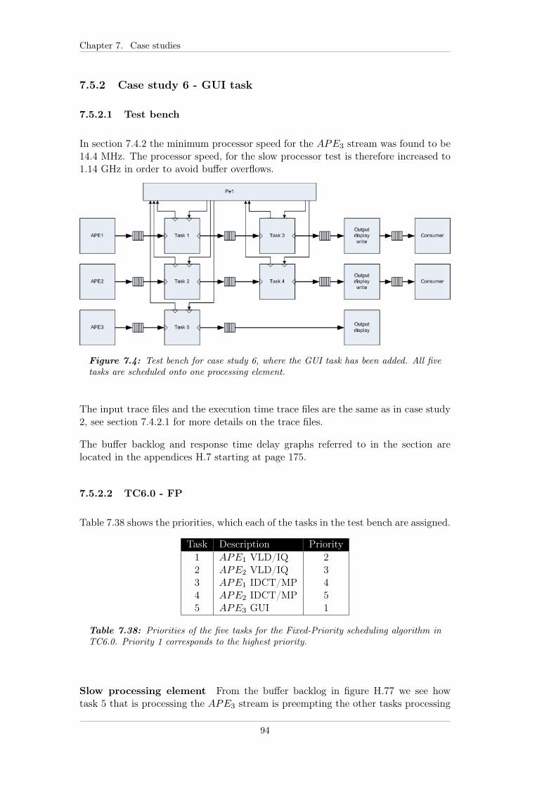
Chapter 7. Case studies
7.5.2 Case study 6 - GUI task
7.5.2.1 Test bench
In section 7.4.2 the minimum processor speed for the APE3 stream was found to be14.4 MHz. The processor speed, for the slow processor test is therefore increased to1.14 GHz in order to avoid buffer overflows.
Figure 7.4: Test bench for case study 6, where the GUI task has been added. All fivetasks are scheduled onto one processing element.
The input trace files and the execution time trace files are the same as in case study2, see section 7.4.2.1 for more details on the trace files.
The buffer backlog and response time delay graphs referred to in the section arelocated in the appendices H.7 starting at page 175.
7.5.2.2 TC6.0 - FP
Table 7.38 shows the priorities, which each of the tasks in the test bench are assigned.
Task Description Priority1 APE1 VLD/IQ 22 APE2 VLD/IQ 33 APE1 IDCT/MP 44 APE2 IDCT/MP 55 APE3 GUI 1
Table 7.38: Priorities of the five tasks for the Fixed-Priority scheduling algorithm inTC6.0. Priority 1 corresponds to the highest priority.
Slow processing element From the buffer backlog in figure H.77 we see howtask 5 that is processing the APE3 stream is preempting the other tasks processing
94

7.5. One processing element
the streams APE1 and APE2. The APE3 stream has some very processing heavyrequest once in a while, which have a clear impact on the two other stream. TheAPE2 stream does however suffer the most, since the tasks processing this streamhave lower priorities.
The response time delay graph in figure H.78 shows how the APE3 stream task hasthe highest priority, and therefore have fairly low delays.
The APE1 stream lost 3 frames, while the APE2 stream lost 9 frames.
Fast processing element The buffer backlog graph in figure H.79 shows a systemthat is capable of servicing the APE1 and APE2 stream sufficiently even for theWCET. The processing heavy request from the APE3 stream does however have anegative impact on the APE1 and APE2 stream.
The response time delays in figure H.80 clearly shows how the APE3 stream hasthe highest priority, followed by the APE1, while the APE2 stream has the lowestpriority.
The APE1 stream did not lose any frames, while the APE2 stream lost 3 frames.
7.5.2.3 TC6.1 - EDF
The deadlines for each of the tasks are set corresponding to their periods as in casestudy 2. Table 7.16 on page 75 contains the deadlines.
Slow processing element The buffer backlog in figure H.81 shows the effect of thefifth task not meeting the deadlines, since the display buffers for both the APE1 andthe APE2 streams at times only are read from. This is caused by the implementationof the EDF scheduler, where the deadline of a task is set to 0 seconds, thereby givingit exclusive rights to the processor until it terminates.
The response time delay in figure H.86 shows how the deadlines of the APE1 streamtasks are shorter, and therefore the scheduler favours the APE1 stream tasks.
The APE1 stream lost 1 frame, while the APE2 stream lost 6 frames.
Fast processing element The buffer backlog and the response time delays inthe figures H.83 and H.84 respectively, show a system that is not fully capable ofservicing the large variability in the APE3 stream. But it does however regain fast.The response time delays for the APE1 are very low, and mostly above 0 when theAPE3 stream sends the processing heavy tokens.
The APE1 stream did not lose any frames, while the APE2 stream lost 2 frames.
95

Chapter 7. Case studies
Parameter Tasks 1 Tasks 2 Task 3 Task 4 Task 5Budget 4 µs 12 µs 15 µs 25 µs 33 msPeriod 26 µs 135 µs 27 µs 135 µs 215 msUtilization 0.15 0.09 0.56 0.19 0.02
Table 7.39: This table contains the CBS parameters for each of the tasks that are inthe test bench. Note that the utilization factors in the table are rounded down to twodecimals.
7.5.2.4 TC6.2 - EDF+CBS
The total utilization factor is 1.14 for the five tasks. The CBS parameters were foundin case study 8.
Slow processing element From the buffer backlog in figure H.85 we see that theCBS parameters are sufficient in order to ensure that the APE2 stream tasks areserviced perfectly. The APE1 stream tasks do however have some problems whenthe APE3 has some processing intensive requests. This is both caused by the APE3
task having a rather large budget, and the APE1 having a small budget.
The response time delay graph in figure H.86 also shows how the APE2 stream tasksare serviced quite well, while the APE1 stream tasks are delayed quite often.
The APE1 stream lost 5 frames, while the APE2 did not lose any frames.
Fast processing element The buffer backlog in figure H.87 shows how both theAPE1 and APE2 stream tasks are serviced very well. The backlog in the APE1
display buffer seldom falls below the initial buffering.
The response time delay graph in figure H.88 shows how the temporal protectionensures that the APE1 and APE2 stream tasks are serviced more or less equally,which is caused by the tasks completing within the given budgets.
Neither the APE1 or APE2 streams lost any frames.
7.5.2.5 TC6.3 - Linux
The task priorities and time slots are the same in this test case as in TC2.3. Table7.18 on page 76 lists the priority and resulting time quanta for the five tasks.
Slow processing element The buffer backlog in figure H.89 shows a very nicescheduling, where the APE1 stream tasks are favoured, but the APE2 stream tasksare also serviced sufficiently often.
Neither stream APE1 or APE2 lost any frames.
96

7.5. One processing element
Fast processing element The buffer backlog in figure H.91 shows that the fourtasks processing the APE1 and APE2 streams are serviced perfectly. The responsetime delays in figure H.92 shows that the APE1 stream tasks have the highest pri-orities, and are in most cases serviced instantly at arrival.
7.5.2.6 Summary
TC Speed Frame Loss (%) Average Response timeAPE1 APE2 APE1 APE2 APE3
6.0 Slow 0.7 2.4 1,485 µs 142,923 µs 8,053 µsFP Fast 0 0.8 304 µs 1,312 µs 6,030 µs6.1 Slow 0.2 1.3 1,041 µs 46,380 µs 1,828,211 µsEDF Fast 0 0.5 281 µs 924 µs 18,076 µs6.2 Slow 1.1 0 37,797 µs 42 µs 15,771 µsCBS Fast 0 0 309 µs 30 µs 12,033 µs6.3 Slow 0 0 21 µs 8,037 µs 1,996,082 µs
Linux Fast 0 0 15 µs 70 µs 25,316 µs
Table 7.40: Summary of the various sub test cases for case study 6. APE1 consist of449 frames, while APE2 consist of 373 frames.
The CBS and the Linux schedulers are the most promising schedulers in this testcase, when looking at the tests with the slow processing element. The CBS schedulinghas a 1.1 % loss of frames, but with very low response time for all the three streams.The Linux scheduler had no frame losses at all, but the response time for the APE3
task i very high, at nearly 2 seconds.
Tables 7.41 and 7.42 shows that the Linux scheduling requires significantly smallerbuffers than the other three scheduling techniques. Two second response time for theAPE3 stream does however seem somewhat long compared to the 16 ms that theCBS scheduling algorithm can deliver. So the final choice is a trade off between chiparea and responsiveness of a task. Changing the priorities in the Linux schedulermight reduce the response time and make this even more attractive.
97

Chapter 7. Case studies
Buffer backlogStream Buffer name
FP EDF CBS LinuxAPE1 t1_input 1,390 1,377 3,648 16
t1_t3_input 2,733 1,800 1 18t3_output 1 1 1 1ape1_con 3,971 3,025 4,934 2,641
APE2 t2_input 312 305 1 148t2_t4_input 2,632 1,410 1 273t4_output 1 1 1 1ape2_con 2,874 1,651 603 603
APE3 t5_input 5 5 5 25t5_output 1 1 1 1
Table 7.41: Buffer backlog for case study 6 with the slow processors.
Buffer backlogStream Buffer name
FP EDF CBS LinuxAPE1 t1_input 1,056 1,055 1,338 14
t1_t3_input 1,305 1,301 1 15t3_output 1 1 1 1ape1_con 2,641 2,641 2,641 2,641
APE2 t2_input 230 231 1 6t2_t4_input 846 495 1 7t4_output 1 1 1 1ape2_con 973 741 603 603
APE3 t5_input 5 5 5 5t5_output 1 1 1 1
Table 7.42: Buffer backlog for case study 6 with the fast processors.
98

7.5. One processing element
7.5.3 Case study 7 - Input with jitter
The test bench from case study 5 is reused, but in this test there is jitter on theinput token generators. Table 7.22 from case study 3 contain the parameters for thetwo input generators.
7.5.3.1 TC7.0 - FP
The four tasks have the same priorities as in TC5.0, and are given in table 7.32 onpage 89.
Slow processing element The buffer backlog in figure H.93 shows how task 1,which is processing the APE1 stream, has the highest priority since the APE1 streamdisplay buffer for the most time at the initial buffering level. The buffer backlog inthe APE2 stream display buffer fluctuates since the tasks processing this streamhave lower priorities.
From the response time delay graph in figure H.94 we see how the APE1 streamtasks have higher priorities and therefore have lower response time delays.
Neither of the two streams lost any frames.
Fast processing element The buffer backlog in figure H.95 shows that the tasksare serviced sufficiently often, since the backlog is never beneath the initial bufferinglevel.
The response time delay again shows that the APE1 stream tasks are favoured overthe APE2 stream tasks, since the response time delay for the APE1 stream is lowest.
No frames were lost in either of the two streams.
7.5.3.2 TC7.1 - EDF
The tasks have the same deadlines as in TC1.1 and are given in table 7.9.
Slow processing element The buffer backlog in figure H.97 shows that the APE1
stream tasks are favoured over the APE2 stream tasks. The APE2 are even servicedworse than when using the FP scheduling algorithm. This is caused by the twoAPE1 stream tasks having the highest priorities, since they have the shortest initialdeadlines, while the two tasks processing the APE2 have the lowest priorities. Thisis not the case for the FP scheduling algorithm where the first tasks processing thetwo streams had higher priorities than the second tasks processing the streams.
The response time delay graph in figure H.98 also shows that the APE1 stream taskshave higher priorities than the APE2 stream tasks.
The APE1 stream did not lose any frames, while the APE2 stream lost 29 frames.
99

Chapter 7. Case studies
Fast processing element The buffer backlog in figure H.99 again simply showsthat the tasks are serviced often enough to maintain the backlog in the display buffersat the initial buffering level.
It is clear from the response time delay graph in figure H.100 that the two tasksprocessing the APE1 stream are favoured over the APE2 stream tasks, since thedelay is much lower than for the APE2 stream. There is even no delay at all forsome of the tokens in the APE1 stream.
No frames were lost for either of the streams.
7.5.3.3 TC7.2 - EDF+CBS
The CBS parameters in this test are based on the average execution time and theperiod of the tasks. Table 7.33 from TC5.2 contains the parameters.
Slow processing element From the buffer backlog in figure H.101 it is clear thatthe CBS parameters for the APE1 do not cover the high intra variability in thestream, while the CBS parameters for the APE2 are sufficient to keep the backlogin the display buffer at the initial buffering level. The graph further indicate thatthe problem is concerned with task 1, since the backlog in the input buffer for theAPE1 stream fluctuates quite at bit.
The response time delay graph in figure H.102 also shows how the delay for theAPE1 stream is significantly larger than for the APE2 stream, which is caused bythe temporal protection that is provided by the CBSs.
None of the streams lost any frames, even though the APE1 stream was close.
Fast processing element The buffer backlog in figure H.103 shows how the CBSparameters are sufficient for the four tasks to complete, since the backlog is constantlyabove the initial buffering level.
The response time delay in figure H.104 shows how the temporal protection ensuresthat the two tasks are more equal, since the APE1 stream also has low delays.
None of the streams lost any frames.
7.5.3.4 TC7.3 - Linux
The tasks priorities in this test case are the same as in TC5.3 and are given in table7.34 on page 91.
100

7.5. One processing element
Slow processing element The buffer backlog in figure H.105 is very similar tothat found when using the EDF scheduling algorithm. This is caused by the timeslots being much larger than the actual processing time, therefore the fairness in thealgorithm is not seen. Further the two tasks processing the APE1 stream have thehighest priorities, as was the case in the EDF algorithm.
The response time delay graph is also very similar to the one found using the EDFalgorithm.
The APE1 stream did not lose any frames, while the APE2 stream lost 29 frames,which is the same as for the EDF scheduling algorithm.
Fast processing element Again both the buffer backlog and the response timedelay graphs in figures H.107 and H.108 are similar to those found using the EDFscheduling algorithm. The APE1 stream tasks are favoured over the APE2 streamtasks, which is caused by the APE1 stream tasks having the highest priorities.
No frame were lost for either of the two streams.
7.5.3.5 Summary
TC Speed Frame Loss (%) Average Response timeAPE1 APE2 APE1 APE2
7.0 Slow 0 0 133 µs 13,487 µsFP Fast 0 0 15 µs 62 µs7.1 Slow 0 7.8 160 µs 77,731 µsEDF Fast 0 0 14 µs 62 µs7.2 Slow 2.4 0 20,311 µs 43 µsCBS Fast 0 0 20 µs 30 µs7.3 Slow 0 7.8 20 µs 78,104 µs
Linux Fast 0 0 14 µs 62 µs
Table 7.43: Summary of the various sub test cases for case study 7. APE1 consist of449 frames, while APE2 consist of 373 frames.
Of the four tests the FP has actually performed best in this case study when usingthe slow processing element. But the CBS might perform better if the budget andperiod are altered. Further the Linux scheduling algorithm will probably also performequally well as the FP, if the priorities of the tasks are set in the same way as in theFP scheduling algorithm.
It is quite clear how the EDF and Linux scheduling algorithms have very similarresults, which is caused by the deadlines in the EDF prioritising the APE1 streamtasks higher than the APE2 stream tasks. This then results in the tasks beingprioritised in more or less the same way, except that the Linux always prioritisestask 3 over task 1, where the EDF is more random. Further the APE2 stream taskswill also have higher priorities using the EDF, once they get near their deadlines.
101

Chapter 7. Case studies
Buffer backlogStream Buffer name
FP EDF CBS LinuxAPE1 t1_input 2 3 2,138 2
t1_t3_input 180 135 1 7t3_output 1 1 1 1ape1_con 2,649 2,646 2,642 2,649
APE2 t2_input 1 2 2 184t2_t4_input 350 1,533 1 1,537t4_output 1 1 1 1ape2_con 603 1,009 604 1,009
Table 7.44: Buffer backlog for case study 7 with the slow processors.
When the fast processing element is used there is no mentionable difference betweenthe four scheduling algorithms.
When evaluating the requirements of the buffer sizes the FP is again preferred, whenusing the slow processing element, while the requirements are more or less the samewhen using the fast processing element.
Buffer backlogStream Buffer name
FP EDF CBS LinuxAPE1 t1_input 1 2 4 1
t1_t3_input 3 2 1 2t3_output 1 1 1 1ape1_con 2,648 2,648 2,648 2,648
APE2 t2_input 1 2 1 2t2_t4_input 7 2 1 4t4_output 1 1 1 1ape2_con 603 603 603 603
Table 7.45: Buffer backlog for case study 7 with the fast processors.
102

7.5. One processing element
7.5.4 Case study 8 - Varying CBS parameters
The six tests in this case study have only been performed using the slow processingelement, since there is very little or no difference, when using the fast processingelement. This test is performed using the test bench in figure 7.4 from case study 6.The speed of the processing element is therefore increased to 1.14 GHz, in order toaccommodate the third stream.
The average processor cycle count for the 58 task request during the 15 secondsperiod is 3,726,974. With the 1.14 GHz processor this will result in an averageexecution time of 3,269 µs. The CBS parameters which are tested in this case studyare based on the average execution time and the average period of the stream APE3.
TC8.0 TC8.1 TC8.2 TC8.3 TC8.4 TC8.5Task Parameter
Budget 4 µs 8 µs 2 µs 4 ns 4 µs 4 µs1 Period 26 µs 52 µs 13 µs 26 ns 26 µs 26 µs
Utilization 0.15 0.15 0.15 0.15 0.15 0.15Budget 12 µs 24 µs 6 µs 12 ns 2.3 µs 12 µs
2 Period 135 µs 270 µs 67.5 µs 135 ns 26 µs 135 µsUtilization 0.09 0.09 0.09 0.09 0.09 0.09Budget 15 µs 30 µs 7.5 µs 15 ns 15 µs 15 µs
3 Period 27 µs 54 µs 13.5 µs 27 ns 27 µs 27 µsUtilization 0.56 0.56 0.56 0.56 0.56 0.56Budget 25 µs 50 µs 12.5 µs 25 ns 4.8 µs 25 µs
4 Period 135 µs 270 µs 67.5 µs 135 ns 26 µs 135 µsUtilization 0.19 0.19 0.19 0.19 0.19 0.19Budget 3.3 ms 6.6 ms 1.65 ms 3.3 µs 399 ns 33 ms
5 Period 215 ms 430 ms 107.5 ms 215 µs 26 µs 215 msUtilization 0.02 0.02 0.02 0.02 0.02 0.15
Table 7.46: This table contains the various parameters for budget and period, whichwere tested in order to find an optimal set-up in case study 8. Note that the time unitsfor task 5 differ from those for tasks 1-4. Further note that the time units in TC 8.3are in ns instead of µs for tasks 1-4, as the other tests. Not all the utilization factorsin the table add up to the total, due to rounding, with only 2 decimals.
The total utilization factors for all the tasks in each of the sub tests 0-4 are 1.00,thus making the system schedulable. The utilization factor for TC8.5 is however1.14, which technically makes the system unschedulable, but since all tasks are softreal-time tasks and the APE3 is not a continuous media stream, this is acceptable.
7.5.4.1 TC8.0
The CBS parameters, budget and period, in this test correspond to the averageexecution times and the average periods of the tasks.
The buffer backlog in figure H.109 shows how the CBS parameters are sufficient forthe APE2 stream, while the intra variability in the APE1 as usual has a negativeeffect, which reduces the performance of the tasks processing the stream.
103

Chapter 7. Case studies
The response time delay in figure H.110 clearly shows how the parameters for theAPE2 stream tasks are acceptable, while the APE1 stream has large delays. TheAPE3 also has some high delays, which is caused by the low utilization factor forthe task that is processing the APE3 stream.
The APE1 stream lost 9 frames, while the APE2 did not lose any frames.
7.5.4.2 TC8.1
Doubling the budget and period of the CBSs did not have any positive effect on thebuffer backlog for the APE1 display buffer. This is caused by the utilization factorstill being the same, and the increased period simply makes the APE1 stream taskswait for a longer time before they are granted access to the processing element again.
The response time delays are better for the APE3 stream, while they are slightlyworse for the APE1 stream, compared to TC8.0.
The frame loss for the APE1 stream is 13, while the APE2 once again did not loseany frames.
7.5.4.3 TC8.2
Halving the budget and period of the CBSs has a positive impact on the bufferbacklog in the APE1 display buffer, while it has a negative effect on the bufferbacklog in the APE2 display buffer.
This is also seen in the response time delay in figure H.114, where the delays are lowfor the APE1 stream, while they are larger for the APE2 stream.
The APE1 stream did not lose any frames, while the APE2 stream lost 29 frames.
7.5.4.4 TC8.3
In this test the budget and period of the CBSs are divided by 1000, which shouldmake the scheduler reschedule the tasks much more often.
The rescheduling of the task causes high fluctuations in the buffers as seen in figureH.115. The scheduler does however have a positive effect, since it provides fairnessthereby giving all the tasks access to the processing element more often.
This is also seen in the response time delays in figure H.116. The delays are howeveron average higher than before, which is caused by the fairness, where the tasks haveto wait quite often for the other tasks also gaining access to the processing element.
None of the streams lost any frames.
104

7.5. One processing element
7.5.4.5 TC8.4
All five tasks have the same period, namely 26 µs. The budgets of each of the taskshave then been scaled in order for the utilization factors to remain the same.
As we have seen in most of the previous tests, the APE1 stream still suffers fromtask 1 having too small an utilization factor, which then makes it unstable. TheAPE2 has a utilisation factor which is sufficient, and therefore has a constant bufferbacklog at the initial buffering level. The buffer backlog graph is given in figureH.117.
The response time delay graph in figure H.118 also shows how the APE2 stream isfavoured over the APE1 stream.
The APE1 stream lost 10 frames, while the APE2 stream did not lose any frames.
7.5.4.6 TC8.5
This is a special case, where the sum of the utilisation factors for the five CBSsis 1.14 which is above 1, and the tasks will therefore not be schedulable accordingto the schedulability analysis. The tasks are aperiodic soft real-time tasks and willtherefore not always spend all of the budget before terminating. With this reasoningwe accept that the summed utilization factor is above 1.
The tasks processing the APE1 and APE2 streams all use the same CBS parametersas in TC8.0, which correspond to the average execution time and period. The fifthtask, which is processing the APE3 stream is given a bandwidth which is a factorof 10 larger than the average execution time. The period of the CBS remains as theaverage period of the APE3 stream. The purpose is to lessen the response time delayof the APE3 stream, without lessening the budget and period of the other tasks.
The buffer backlog in figure H.119 shows how the APE1 tasks are not servicedregularly, due to the APE3 stream. The APE2 stream is however relative unaffected,which probably is caused by the stream having a larger period, and therefore moretolerable to the bursts from the APE3 stream.
The higher bandwidth for the APE3 stream has further resulted in the stream havinga considerably lower response time delay than in the previous tests. The responsetime delay graph is shown in figure H.120.
The APE1 stream lost 5 frames, while the APE2 did not lose any frames.
7.5.4.7 Summary
The six tests performed in this case study produce very different results. The bestresult from the tests is a subjective matter, where the user either must choose to
105

Chapter 7. Case studies
prefer the least amount of frames losses or low response time of the tasks. The TC8.3produced no frame losses, but this was at the expense of the APE3 stream, whichhad an average response time of 2 seconds, which is very high.
The TC8.5 seems like the over all winner, since it has a very low amount of framelosses, and the average response time for the APE3 is also very low. A static schedul-ing analysis would however conclude that the system is unschedulable. But we acceptthis based on the fact that the APE3 stream is highly aperiodic, and that all of thefive tasks are soft real-time tasks.
TC Frame Loss (%) Average Response timeAPE1 APE2 APE1 APE2 APE3
8.0 2.0 0 19,643 µs 42 µs 1,126,809 µs8.1 2.9 0 36,249 µs 184 µs 70,675 µs8.2 0 7.8 35 µs 124,573 µs 230,709 µs8.3 0 0 1,128 µs 2,905 µs 2,014,329 µs8.4 2.2 0 16,089 µs 41 µs 1,498,562 µs8.5 1.1 0 37,797 µs 42 µs 15,771 µs
Table 7.47: Summary of the various sub test cases for case study 8. APE1 sends atotal of 449 frames, while APE2 sends 373 frames.
In terms of the buffer requirements TC8.3 requires the least buffer sizes, while TC8.5is among the set-ups which require the largest buffers. The TC8.5 is however seenas the test which has the best performance.
Buffer backlogStream Buffer name
TC8.0 TC8.1 TC8.2 TC8.3 TC8.4 TC8.5APE1 t1_input 3,275 3,275 228 362 2,912 3,648
t1_t3_input 1 1 5 274 1 1t3_output 1 1 1 1 1 1ape1_con 3,252 4,253 2,641 2,641 2,890 4,934
APE2 t2_input 1 264 972 147 1 1t2_t4_input 1 291 2,261 227 1 1t4_output 1 1 1 1 1 1ape2_con 603 604 972 603 603 603
APE3 t5_input 20 5 7 25 23 5t5_output 1 1 1 1 1 1
Table 7.48: Buffer backlog for case study 8 with the slow processor.
7.6 Conclusion
The general conclusion from the case studies is that the CBS is an efficient schedulingalgorithm for soft real-time systems, when the system just meets the average resourcerequirements. This is caused by the fairness, which the CBS provides due to the
106

7.6. Conclusion
Case Study Response time BufferSlow Fast Slow Fast
1 CBS - FP -2 CBS CBS CBS CBS3 CBS - FP -5 CBS CBS FP/EDF -6 CBS CBS CBS Linux7 FP CBS FP -
Table 7.49: This table shows the preferred scheduling algorithm from each of the casestudies, except for case study 4 and 8. The cases where there is no name in the cellsimply means that there is very little difference.
temporal protection characteristics. The fairness of the Linux O(1) scheduler wasnot really experienced, since the task execution times in most cases, are below thewindow sizes that they were assigned.
Table 7.49 shows the scheduling techniques which performed best for each of the testcases. This is based both on the frame losses, buffer backlog and response times ofthe streams. Most of the test cases with the fast processing elements did not showany notable difference in the QoS, and either of the four scheduling schemes could beused. The buffer size requirements did however in many cases, for the fast elements,favour one scheduling scheme over the others.
Case studies 4 and 8 did not show any definitive answer to finding the optimalvalues for the CBS parameters budget and period. Case study 4 resulted with thebest parameters in TC4.3, where the budget and period are 1000 times shorter thanthe average execution time and period for each task. Case study 8 did on the otherhand show that the best values for the parameters are setting the budget 10 timeslonger than the average execution time, while the period was unchanged.
The CBS parameters in case studies 1, 3, 5 and 6 all use the standard parameters,where the budget and period are respectively assigned as the average execution timeand the average period of the tasks. The results for the CBS test cases in thesecase studies are likely to be further improved with more optimal values for the CBSparameters.
107

Chapter 7. Case studies
108

Chapter 8
Conclusion
This thesis presented two types of variability for multimedia in terms of executiontime. These are intra and inter variability, where intra variability is within eachstream, while inter variability is across different streams. The inter variability isgreatest for media streams with different characteristics in terms of resolution andframe rate.
The DIstributed Multimedia Application Simulator (DiMAS) was implemented, whichis a C++ library. DiMAS is used for creating a design level simulator, which modelsa given multimedia system. This could for example be a set-top box or a DVD player.The simulator can be used when designing new multimedia appliances, where theresources must be kept low, in order to limit cost or power consumption. The costlyand time consuming prototyping process can therefore be postponed or completelyremoved in the design phase.
The DiMAS library is able to model processing elements with four different types ofscheduling techniques. These four techniques are Fixed-Priority, Earliest DeadlineFirst, Constant Bandwidth Server and the Linux O(1) schedulers. The DiMAS li-brary is an extension of the Pesimdes library, which is a simulation framework forhard real-time systems. The Fixed-Priority and the Earliest Deadline First schedul-ing techniques were already part of the Pesimdes library. The Constant BandwidthServer and the Linux O(1) schedulers are new implementations.
The variability in terms of execution time for a multimedia stream is modelled usinga trace file, which either contains the processor cycles or the actual execution timesgiven in a user specified time unit.
The MPEG video stream was chosen as the main multimedia stream to be used inthe examples and discussions throughout the thesis. This was partly caused by theobvious partitioning of tasks in the decoding algorithm, and partly by video havinga strong association towards multimedia.
Eight case studies were created to show some examples of how the DiMAS librarycan be used. The examples are kept simple with two multimedia streams, and insome cases with an additional stream, which is highly aperiodic. The case studieseither use test benches with one and two processing elements.
109

Chapter 8. Conclusion
The case studies showed a great difference between the four scheduling algorithms.This was especially visible when the processing elements were designed based on theaverage execution times of the tasks. The over designed test benches did howeverresult in very similar results for each of the four scheduling algorithms. In generalthe Constant Bandwidth Server scheduling algorithm performed in most cases betterthan the other three. The performance was evaluated based both on frame lossesand the average response times. The temporal protection in the CBS schedulingalgorithm ensured that all tasks were given a fair share of the processing element.The Linux O(1) scheduling algorithm was in most cases not able to provide thefairness it should, since the tasks finished within the assigned time slots.
Case studies 4 and 8 showed that the parameters budget and period of the CBSshave a big influence on the performance. And simply using the average values of theexecution time and period for each task is not necessarily the best choice. The twotests ended with one performing best with very low budget and period, while thethe other performed best with a high value for the budget while the value for theperiod was unchanged. There is from these tests no way of saying how the optimalparameters are determined without performing many simulations.
8.1 Future work
An obvious extension of the simulation library, would be adding new schedulingalgorithms. The modularity of the library makes this a fairly easy task.
Modelling a multimedia system can be very complicated using DiMAS, if there aremany tasks in the system. An abstraction from the C-code would therefore bepreferable, either using a graphical user interface with drag and drop functionality,or using a description file for example in xml format.
The current version of the simulator library is able to model the variable executiontime using trace files, where each line in the file correspond to a task request. Itwould however be preferable to also have the possibility of modelling the variabilitybased on a probability distribution.
Currently network connections are modelled at the input generators. This couldhowever also be modelled in the test bench, in order to be able to model a full dis-tributed multimedia system, where amplifier, dvd, speakers, television and speakersall communicate using a wireless connection.
110

Bibliography
[ZL02] Vladimir D. Zivković, Paul Lieverse: An Overview of Method-ologies and Tools in the Field of System-Level Design, 2002.
[SSTutorV4] SimpleScalar LLC: Simple Tutorial v4, Cited: 25-6-08, http://www.simplescalar.com/docs/simple_tutorial_v4.pdf.
[SShome] SimpleScalar LLC: SimpleScalar homepage, http://www.simplescalar.com/
[MY07] Matt T. Yourst: PTLsim: A Cycle Accurate Full System x86-64 Microarchitectural Simulator, 2007, http://www.ptlsim.org/papers/PTLsim-ISPASS-2007.pdf.
[ALE02] Todd Austin, Eric Larson, Dan Ernst: SimpleScalar: An In-frastructure for computer System Modeling, IEEE 2002.
[BD04] David c. Black, Jack Donovan: SystemC: From the Ground Up,Springer 2004
[GLMS02] Thorsten Grötker, Stan Liao, Grant Martin, Stuart Swan:System Design with SystemCtm, Springer 2002
[ML05] Marco Lohse: Network-Integrated Multimedia Middleware, Servicesand Applications, Saarbrücken University, 2005
[MPEGOrg] MPEG Organization: http://www.mpeg.org/
[TN95] Tudor P. N.: MPEG-2 VIDEO COMPRESSION, 1995, http://www.bbc.co.uk/rd/pubs/papers/paper_14/paper_14.shtml
[SimicsDS] Virtutech: Simics: Virtualized Software Development - Data Sheet,http://www.virtutech.com/
[SimicsWP] Virtutech: Virtualized Software Development, http://www.virtutech.com/files/whitepapers/wp_simics.pdf
[ACH98] Christina Aurrecoechea, Andrew T. Campbell, LindaHauw: A Survey of QoS Architectures, Columbi University, Springer-Verlag, 1998.
[JN04] Jin Jingwen, Klara Nahrstedt: QoS Specification Languages forDistributed Multimedia Applications: A Survey and Taxonomy, Uni-versity of Illinois at Urbana-Champaign, IEEE, 2004.
111
Bibliography
[MVM07] Shankar Mahadevan, Kashif Virk, Jan Madsen: ARTS: ASystemC-based frame work for multiprocessor System-on-Chip mod-elling, Technical University of Denmark, 2007.
[BMP98] Andy C. Bavier, A. Brady Montz, Larry L. Peterson: Pre-dicting MPEG Execution Times, The University of Arizona, 1998.
[SGG09] Abraham Silberschatz, Peter Baer Galvin, Greg Gagne:Operating System Concepts, Eighth Edition, John Wiley & Sons inc.,2009
[BLAC05] Giorgio Buttazzo, Giuseppe Lipari, Luca Abeni and MarcoCaccamo: Soft Real-Time Systems - Predictability vs. Efficiency,Springer, 2005
[SP06] Simon Perathoner: Evaluation and Comparison of PerformanceAnalysis Methods for Distributed Embedded Systems, Swiss Federal In-stitute of Technology, Zürich, 2006
[MH07] Max Hailperin: Operating Systems and Middleware: SupportingControlled Interaction, 2007. Online resource to update information inthe book: http://gustavus.edu/+max/os-book/updates/CFS.html
[RR02] Rassol Raissi: The Theory Behind MP3, 2002, http://www.mp3-tech.org/programmer/docs/mp3_theory.pdf
[BP00] Karlheinz Brandenburg, Harald Popp: An Introduction toMPEG Layer-3, Fraunhofer Instittut Für Integrierte Schaltungen(IIS), 2000
[AM05] Alexander Maksyagin: Modeling Multimedia Workloads for Em-bedded System Design, phd. thesis, Institut für Technishe Informaticund Kommunikationsnetze, Eidgenössische Technische HochschuleZürich, 2005.
112

Appendix A
Developed utilities
A.1 BreakDiff
The breakDiff utility is used for extracting the cycle counts between up to 10 break-point sets from the trace files generated by the modified SimpleScalar tool set pre-sented in section 6. The purpose of the utility is to calculate the time differencebetween the two breakpoints in each breakpoint set. The difference is stored in anew file, and is a number for either the instruction count or the cycle count betweenthe two breakpoints. The sim-outorder simulator from SimpleScalar generates traceswith processor cycle counts, while the rest of the simulators generate the traces basedon the instruction count.
The utility takes a file name and a sequence of numbers defining the breakpointsas parameters. The program then outputs a file for each breakpoint set and anadditional file which contains all the breakpoint data, and a summary section at theend. The parameters are structured as follows:
breakDiff <file name> <# breakpoint sets> <start> <end> <name>[<start> <end> <name>]
A.2 mpeg2stat
The MPEG stat application is based on the MPEG open source implementationof the MPEG decoder at [MPEGOrg]. The open source implementation is alreadyable to extract the header information in the various parts of an MPEG video file.The mpeg2stat application can either print a summary table containing the mostinteresting characteristics of a file to the terminal, or create a trace file where thetype of frame each macroblock is part of. The frame type can either be I, P or Bframes as explained in section 2.1.1. The last option is to make a full trace containingmost of the header information in the MPEG video file.
The command for the mpeg2stat application is:mpeg2stat -b <mpeg video filename> -v<level>
113

Appendix A. Developed utilities
Where
-v0 Prints a summary of the MPEG video file to the terminal
-v1 Prints the same short summary as for the -v0 option. Further the applicationgenerates a trace file, where the type of each of frame is logged. The valuesrange from 1-3 corresponding to I, P and B frames. The summary table isappended to the trace files, which is based on the input file name and suffixedwith .FrameTrace.
-v2 Prints out many details regarding a video file to the terminal. No additionaltrace file is created. This is only useful if very specific information is required.
A.3 VCD Parser
The VCDParser parses a vcd (Value Change Dump) file and writes a new morereadable file, which easily can be plotted using gplot. The parser can either be usedsimply with the file name as input thereby extracting all the variables in the file, orthe specific variables can be specified as parameters thereby only extracting a subsetof the variables in the file.
The first column in the output file is the time, while the consecutive columns eachrepresent a variable. There is a row of data for all variables each time just one ofthe variables changes value. If events for the variables are important then the utilityneeds to be run once for each variable, and then saving one file for each variable.This is not a feature of the VCDParser, but can easily be done using a script.
114

Appendix B
Input generator class diagram
115

Appendix B. Input generator class diagram
Figure
B.1:
Class
diagramof
thevarious
inputtoken
generatorsthat
canbe
usedin
theDiM
ASAPI.
116

Appendix C
Users guide
The DiMAS API requires that the SystemC library is compiled and working correctly.SystemC is downloaded for free at the official home page: http://www.systemc.org/downloads/standards/.
The DiMAS API has only been tested on the Linux platform, but should also work onWindows platforms. The DiMAS library was implemented with the KDevelopmentprogramming environment, using an automake project. The SystemC library mustbe referenced as described in the KDevelop documentation, in order for the DiMASto compile correctly.
Alternative the DiMAS library can be compiled in the terminal. In order for thisto be possible the include paths in the two files /Makefile.am and /src/Makefile.ammust be updated. These lines must be either the absolute or the relative path tothe folder containing the header files for SystemC. Further the LDFLAGS must beused in the make command, where the path to the compiled SystemC library file islocated1.
Test benches are typically created in the main.cpp file.
It can be quite complicated to create a large test bench with many tasks and pro-cessing elements. Therefore it is advisable to make a diagram, where all the modulesin the test bench are named, and use a suitable naming convention.
A test bench typically include the following modules.
• Input generators
• Tasks
• Resources (Processing elements with a specific scheduling algorithm)
• Buffers1There is definitely an easier way, but this is not known by the author.
117

Appendix C. Users guide
• Display devices
• Consumers
If a specific multimedia set-up is tested using different types of resources, it is advis-able to partition the test bench into three parts.
Physical test bench Here the modules that are common for the tests are created.These include input generators, tasks, buffers, display devices and Consumers.Further the connections between tasks and buffers are done here.
Resource This part is created for each of the scheduling techniques which shouldbe tested. The resources that should be used in the test are initialized, andthe tasks in the test bench are assigned the resources. Further resource specificoperations are performed. This could for example be assigning the correct tracefiles, and processor speeds. If the buffer tracing should be used the trace file isopened and the buffers are added to the trace file. Further all the output filesfor the display and consumer modules are given in this part.
Post processing This part contains all the operations, which should be performedafter simulation. These include closing the vcd file. Further calling the func-tions write_latencies and traceSummary for the display and Consumer mod-ules respectively.
Listings C.1 shows an example of a test bench, where the three partitions are in-cluded. The code in the listing correspond to the test bench in figure C.1.
Figure C.1: Example of a test bench with two processing elements and two continuousmedia streams.
Listing C.1: Example of a test bench1 #define MAXBUFFER 200002
3 bool verbose = false;4
5 int sc_main (int argc , char *argv []) {6 // initialize the random number generator7 // srand (-24);8
9 /* ===============================================10 Test bench for TC111 ===============================================
118

12 2 processing elements13 2 multimedia files14 =============================================== */15
16 // Token generators17 // input_periodic ape1_generator (" ape1_input", sc_time (25252 , SC_NS), "
TC1_ape1_input_tracer.tra");18 // input_periodic ape2_generator (" ape2_input", sc_time (133332 , SC_NS), "
TC1_ape2_input_tracer.tra");19 input_from_trace ape1_generator("ape1_input", "TC1_ape1_input_tracer.tra",
SC_PS); // ~30 fps *1320mb /second20 input_from_trace ape2_generator("ape2_input", "TC1_ape2_input_tracer.tra",
SC_PS); // ~25 fps *300mb / second21
22 // Processing Element 1 with two tasks23 task t1("ape1_vldIq");24 task t2("ape2_vldIq");25 // Processing Element 2 with two tasks26 task t3("ape1_idctMp");27 task t4("ape2_idctMp");28
29 // Buffers30 my_sc_fifo <event_token > t1_input(MAXBUFFER);31 my_sc_fifo <event_token > t2_input(MAXBUFFER);32 my_sc_fifo <event_token > t1_t3_input(MAXBUFFER);33 my_sc_fifo <event_token > t2_t4_input(MAXBUFFER);34 my_sc_fifo <event_token > t3_output(MAXBUFFER);35 my_sc_fifo <event_token > t4_output(MAXBUFFER);36 my_sc_fifo <event_token > ape1_consume(MAXBUFFER);37 my_sc_fifo <event_token > ape2_consume(MAXBUFFER);38
39 // Statistics40 output_display_write ape1_display("ape1_O");41 output_display_write ape2_display("ape2_O");42
43 // Consumers44 Consumer ape1_con("ape1_consumer", 1320, sc_time (33332 , SC_US));45 Consumer ape2_con("ape2_consumer", 300, sc_time (40, SC_MS));46
47 // Buffer Mappings48 // ape1 - Short period multimedia task49 cout << "Connecting ape1 streams ...";50 ape1_generator.out(t1_input);51 t1.in[0]( t1_input);52 t1.out [0]( t1_t3_input);53 t3.in[0]( t1_t3_input);54 t3.out [0]( t3_output);55 ape1_display.in(t3_output);56 ape1_display.out(ape1_consume);57 ape1_con.in(ape1_consume);58 cout << "Success" << endl;59
60 // ape2 - Long period multimedia task61 cout << "Connecting ape2 streams ...";62 ape2_generator.out(t2_input);63 t2.in[0]( t2_input);64 t2.out [0]( t2_t4_input);65 t4.in[0]( t2_t4_input);66 t4.out [0]( t4_output);67 ape2_display.in(t4_output);68 ape2_display.out(ape2_consume);69 ape2_con.in(ape2_consume);70 cout << "Success" << endl;71
72 timeStatus timer("TimeStatus", sc_time(1, SC_SEC));73
74 time_t timeStart , timeEnd;75 struct tm * timeInfo;76
77 /* ===============================================
119

Appendix C. Users guide
78 Test 10 TC1.079 ===============================================80 Fixed Priority Scheduling81 2 multimedia files82 =============================================== */83
84 // IDs for Pe185 #define T1_ID 086 #define T2_ID 187 // IDs for Pe288 #define T3_ID 089 #define T4_ID 190
91 // Fixed -Priority scheduling for Pe192 resource_n_tasks_fixed_priority_preemptive pe_1("CPU1", 2); // Two tasks93 pe_1.setProcessorSpeed (270000000.0); // 270 MHz / 860 MHz94 pe_1.assign_task(t1 , T1_ID , SC_ZERO_TIME , 1);95 pe_1.assign_task(t2 , T2_ID , SC_ZERO_TIME , 2);96
97 pe_1.setRunMode(T1_ID , 2); // Cycle time trace98 pe_1.setInputTraceFile(T1_ID , "TC1_ape1_0_exect.tra", 1); // Trace data in
second column99 pe_1.setCycleMultiplier(T1_ID , 0.557); // ~inst to cycles
100 pe_1.setRunMode(T2_ID , 2); // Cycle time trace101 pe_1.setInputTraceFile(T2_ID , "TC1_ape2_0_exect.tra", 1); // Trace data in
second column102 pe_1.setCycleMultiplier(T2_ID , 0.891); // ~inst to cycles103
104
105 // Fixed -Priority scheduling for Pe2106 resource_n_tasks_fixed_priority_preemptive pe_2("CPU2", 2); // Two tasks107 pe_2.setProcessorSpeed (860000000.0); // 860 MHz / 1.5 GHz108 pe_2.assign_task(t3 , T3_ID , SC_ZERO_TIME , 1);109 pe_2.assign_task(t4 , T4_ID , SC_ZERO_TIME , 2);110
111 pe_2.setRunMode(T3_ID , 2); // Cycle time trace112 pe_2.setInputTraceFile(T3_ID , "TC1_ape2_1_exect.tra", 1); // Trace data in
second column113 pe_2.setCycleMultiplier(T3_ID , 0.139); // ~inst to cycles114 pe_2.setRunMode(T4_ID , 2); // Cycle time trace115 pe_2.setInputTraceFile(T4_ID , "TC1_ape2_1_exect.tra", 1); // Trace data in
second column116 pe_2.setCycleMultiplier(T4_ID , 0.244); // ~inst to cycles117
118 // Trace file119 sc_trace_file *tracefile;120 tracefile = sc_create_vcd_trace_file("TC1_0_buffers");121
122 t1_input.logger_trace(tracefile , "t1_input", "010");123 t2_input.logger_trace(tracefile , "t2_input", "010");124 t1_t3_input.logger_trace(tracefile , "t1_t3_input", "010");125 t2_t4_input.logger_trace(tracefile , "t2_t4_input", "010");126 t3_output.logger_trace(tracefile , "t3_output", "010");127 t4_output.logger_trace(tracefile , "t4_output", "010");128 ape1_consume.logger_trace(tracefile , "ape1_con", "010");129 ape2_consume.logger_trace(tracefile , "ape2_con", "010");130
131 ape1_display.setOutputTraceFile("TC1_0_ape1_display.tra");132 ape2_display.setOutputTraceFile("TC1_0_ape2_display.tra");133
134 ape1_con.setTraceFile("TC1_0_ape1_con.tra");135 ape2_con.setTraceFile("TC1_0_ape2_con.tra");136
137 time(& timeStart);138 timeInfo = localtime (& timeStart);139
140 cout << "Starting simulation @ " << asctime(timeInfo) << endl;141 sc_start (15, SC_SEC);142
143 ofstream sumFile("TC1_0_sum_270M_860M.txt");
120

144 // ofstream sumFile (" TC1_0_sum_860M_1500M.txt");145 sumFile << "Simulation summary for test case TC1_0" << endl;146 sumFile << "Pe1: 270 MHz\t Pe2: 860 MHz" << endl << endl;147 // sumFile << "Pe1: 860 MHz\t Pe2: 1.5 GHz" << endl << endl;148
149
150 /* ===============================================151 Post processing152 =============================================== */153
154 time(& timeEnd);155 timeInfo = localtime (& timeEnd);156 cout << "Simulation ended @ " << asctime(timeInfo) << endl;157 cout << "Simulation time was: "158 << (difftime(timeEnd , timeStart) / 60) << " minutes" << endl;159
160 sc_close_vcd_trace_file(tracefile);161
162 ape1_display.write_latencies("ape1_input");163 ape2_display.write_latencies("ape2_input");164
165 cout << "Lost frame for ape1: " << ape1_con.getFails () << " / "166 << ape1_con.getSuccess () + ape1_con.getFails () << endl;167 cout << "Lost frame for ape2: " << ape2_con.getFails ()168 << " / " << ape2_con.getSuccess () + ape2_con.getFails () << endl;169
170 ape1_con.traceSummary ();171 ape2_con.traceSummary ();172
173 cout << "count from ape1: " << ape1_generator.getCount () << endl;174 cout << "count from ape2: " << ape2_generator.getCount () << endl;175
176 cout << "Task 1: " << t1.input_count << "/" << t1.output_count << endl;177 cout << "Task 2: " << t2.input_count << "/" << t2.output_count << endl;178 cout << "Task 3: " << t3.input_count << "/" << t3.output_count << endl;179 cout << "Task 4: " << t4.input_count << "/" << t4.output_count << endl;180
181 pe_1.printCounts ();182 pe_2.printCounts ();183
184 sumFile << "Lost frames" << endl;185 sumFile << "Lost frame for ape1: " << ape1_con.getFails ()186 << " / " << ape1_con.getSuccess () + ape1_con.getFails () << endl;187 sumFile << "Lost frame for ape2: " << ape2_con.getFails ()188 << " / " << ape2_con.getSuccess () + ape2_con.getFails () << endl;189
190 sumFile << endl << "Latencies" << endl;191 sumFile << "APE1: "192 << "\tmin: " << ape1_display.getminlatency("ape1_input")193 << "\tavg: " << ape1_display.getavglatency("ape1_input")194 << "\tmax: " << ape1_display.getmaxlatency("ape1_input")195 << endl;196 sumFile << "APE2: "197 << "\tmin: " << ape2_display.getminlatency("ape2_input")198 << "\tavg: " << ape2_display.getavglatency("ape2_input")199 << "\tmax: " << ape2_display.getmaxlatency("ape2_input")200 << endl;201
202 sumFile << endl << "Token counts" << endl;203 sumFile << "Task 1: " << t1.input_count << "/" << t1.output_count << endl;204 sumFile << "Task 2: " << t2.input_count << "/" << t2.output_count << endl;205 sumFile << "Task 3: " << t3.input_count << "/" << t3.output_count << endl;206 sumFile << "Task 4: " << t4.input_count << "/" << t4.output_count << endl;207
208 sumFile << endl << "Max. buffer backlogs" << endl;209 sumFile << "t1_input: " << t1_input.getmaxbacklog () << endl;210 sumFile << "t1_t3_input: " << t1_t3_input.getmaxbacklog () << endl;211 sumFile << "t3_output: " << t3_output.getmaxbacklog () << endl;212 sumFile << "ape1_con: " << ape1_consume.getmaxbacklog () << endl;213 sumFile << "t2_input: " << t2_input.getmaxbacklog () << endl;
121

Appendix C. Users guide
214 sumFile << "t2_t4_input: " << t2_t4_input.getmaxbacklog () << endl;215 sumFile << "t4_output: " << t4_output.getmaxbacklog () << endl;216 sumFile << "ape2_con: " << ape2_consume.getmaxbacklog () << endl;217 sumFile.close();218
219 return 0;220 }
122

Appendix D
Multimedia data files
D.1 MPEG-2 files
Presents a table with the most interesting characteristics of the various MPEG filesused in this thesis.
123
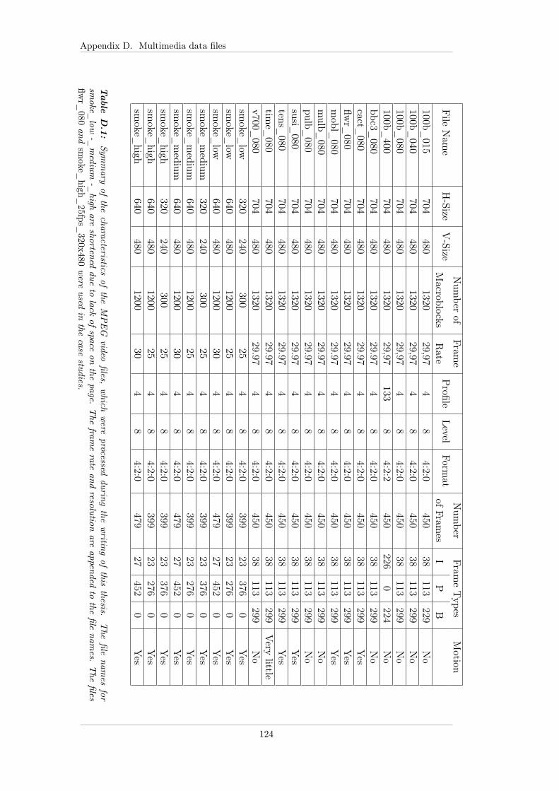
Appendix D. Multimedia data files
Num
berof
Frame
Num
berFram
eTypes
Motion
File
Nam
eH-Size
V-Size
Macroblocks
Rate
Profile
LevelForm
atof
Frames
IP
B100b_
015704
4801320
29,974
84:2:0
45038
113229
No
100b_040
704480
132029,97
48
4:2:0450
38113
299No
100b_080
704480
132029,97
48
4:2:0450
38113
299No
100b_400
704480
132029,97
1338
4:2:2450
2260
224No
bbc3_080
704480
132029.97
48
4:2:0450
38113
299No
cact_080
704480
132029.97
48
4:2:0450
38113
299Yes
flwr_
080704
4801320
29.974
84:2:0
45038
113299
Yes
mobl_
080704
4801320
29.974
84:2:0
45038
113299
Yes
mulb_
080704
4801320
29.974
84:2:0
45038
113299
No
pulb_080
704480
132029.97
48
4:2:0450
38113
299No
susi_080
704480
132029.97
48
4:2:0450
38113
299Yes
tens_080
704480
132029.97
48
4:2:0450
38113
299Yes
time_
080704
4801320
29.974
84:2:0
45038
113299
Very
littlev700_
080704
4801320
29.974
84:2:0
45038
113299
No
smoke_
low320
240300
254
84:2:0
39923
3760
Yes
smoke_
low640
4801200
254
84:2:0
39923
2760
Yes
smoke_
low640
4801200
304
84:2:0
47927
4520
Yes
smoke_
medium
320240
30025
48
4:2:0399
23376
0Yes
smoke_
medium
640480
120025
48
4:2:0399
23276
0Yes
smoke_
medium
640480
120030
48
4:2:0479
27452
0Yes
smoke_
high320
240300
254
84:2:0
39923
3760
Yes
smoke_
high640
4801200
254
84:2:0
39923
2760
Yes
smoke_
high640
4801200
304
84:2:0
47927
4520
Yes
Table
D.1:
Symmary
ofthe
characteristicsof
theMPEG
videofiles,
which
were
processedduring
thewriting
ofthis
thesis.The
filenam
esfor
smoke_
low-_
medium
-_high
areshortened
dueto
lackof
spaceon
thepage.
The
framerate
andresolution
areappended
tothe
filenam
es.The
filesflw
r_080
andsm
oke_high_
25fps_320x480
were
usedin
thecase
studies.
124

D.1. MPEG-2 files
File
Nam
eDecod
eFram
eVLD
/IQ
IDCT/M
PMin
Max
Min
Max
Min
Max
100b
_01
515
0.54
0.16
015
2.25
2.80
92.69
912
.029
109.27
411
8.87
210
0b_04
015
0.58
9.96
915
2.81
7.21
32.69
912
.029
109.27
412
0.88
410
0b_08
015
0.58
9.96
915
2.11
6.25
62.69
912
.029
109.27
411
3.22
410
0b_40
020
0.23
3.12
920
2.06
3.08
93.39
716
.023
145.08
214
8.28
8bb
c3_08
015
0.62
0.66
217
4.83
0.13
42.69
941
.785
109.06
912
4.77
8cact_08
015
6.41
8.24
617
2.07
8.66
52.70
043
.129
109.46
412
8.11
2flw
r_08
015
9.33
1.31
717
3.08
5.53
62.69
946
.205
109.38
112
8.15
8mob
le_08
015
1.79
3.18
417
4.48
0.84
52.69
940
.561
109.27
412
8.09
5mulb_
080
150.58
5.28
916
1.19
6.21
92.69
914
.137
109.24
211
6.58
9pu
lb_08
015
0.35
7.31
915
0.62
2.58
02.69
911
.849
109.25
811
3.21
6susi_08
016
0.52
7.65
017
7.30
6.07
32.70
341
.292
109.42
112
8.11
9tens_08
015
6.83
3.90
817
1.95
3.94
32.69
946
.759
109.33
812
8.15
4time_
080
156.83
3.90
817
1.95
3.94
32.69
946
.759
109.33
812
8.15
4sm
oke_
low_25
fps_
320x
240
35.130.922
38.579
.820
2.11
535
.880
108.74
211
8.69
0sm
oke_
low_25
fps_
640x
480
138.07
0.27
915
1.19
1.18
92.11
530
.421
108.39
711
8.71
2sm
oke_
low_30
fps_
640x
480
137.81
6.20
315
1.19
1.18
92.11
530
.421
108.39
711
8.71
2sm
oke_
medium_25
fps_
320x
240
36.040.717
38.643
.062
2.11
540
.813
109.25
311
8.65
2sm
oke_
medium_25
fps_
640x
480
139.62
4.37
015
1.19
1.18
92.11
530
.330
108.76
511
8.73
6sm
oke_
medium_30
fps_
640x
480
138.87
3.69
815
1.19
1.18
92.11
530
.330
108.39
711
8.74
6sm
oke_
high
_25
fps_
320x
240
36.968.720
39.910
.160
2.11
546
.255
109.25
011
8.64
9sm
oke_
high
_25
fps_
640x
480
142.08
4.29
215
2.25
9.56
52.11
530
.579
108.95
211
8.71
7sm
oke_
high
_30
fps_
640x
480
141.44
3.69
515
1.19
1.18
92.11
530
.330
108.49
311
8.72
3
125

Appendix D. Multimedia data files
126

Appendix E
Commands for generating traces
The commands below are used in the interactive debugger to configure the debuggerto log three breakpoint sets, as described in section 6.
1 tracefile profile_block_xxx.txt2 dbreak 0x0204b528 w3 dbreak 0x0204b52c w4 dbreak 0x0204b530 w5 dbreak 0x0204b534 w6 dbreak 0x0204b538 w7 dbreak 0x0204b53c w8 tracecomm trace_performed_19 .01.09 _by_Rolf_Kristensen9 tracecomm breakpoint1 :0 x0204b528_global_start_decodePic
10 tracecomm breakpoint2 :0 x0204b52c_global_end_decodePic11 tracecomm breakpoint3 :0 x0204b530_global_start_vldIq12 tracecomm breakpoint4 :0 x0204b534_global_end_vldIq13 tracecomm breakpoint5 :0 x0204b538_global_start_idctMp14 tracecomm breakpoint6 :0 x0204b53c_global_end_idctMp15 tracecomm bp1_and_bp2_encapsulates_decoding_of_one_frame.16 tracecomm bp3_and_bp4_encapsulates_the_VLD/IQ_part_of_the_decoding_process17 tracecomm bp5_and_bp6_encapsulates_the_IDCT/MP_part_of_the_decoding_process18 tracecomm simulation_is_performed_using_the_sim -profile_simulator19 tracecomm simulation_is_performed_on_the_file_xxx20 quietTrace on21 cont
Where xxx is the name of the multimedia file.
127

Appendix E. Commands for generating traces
128
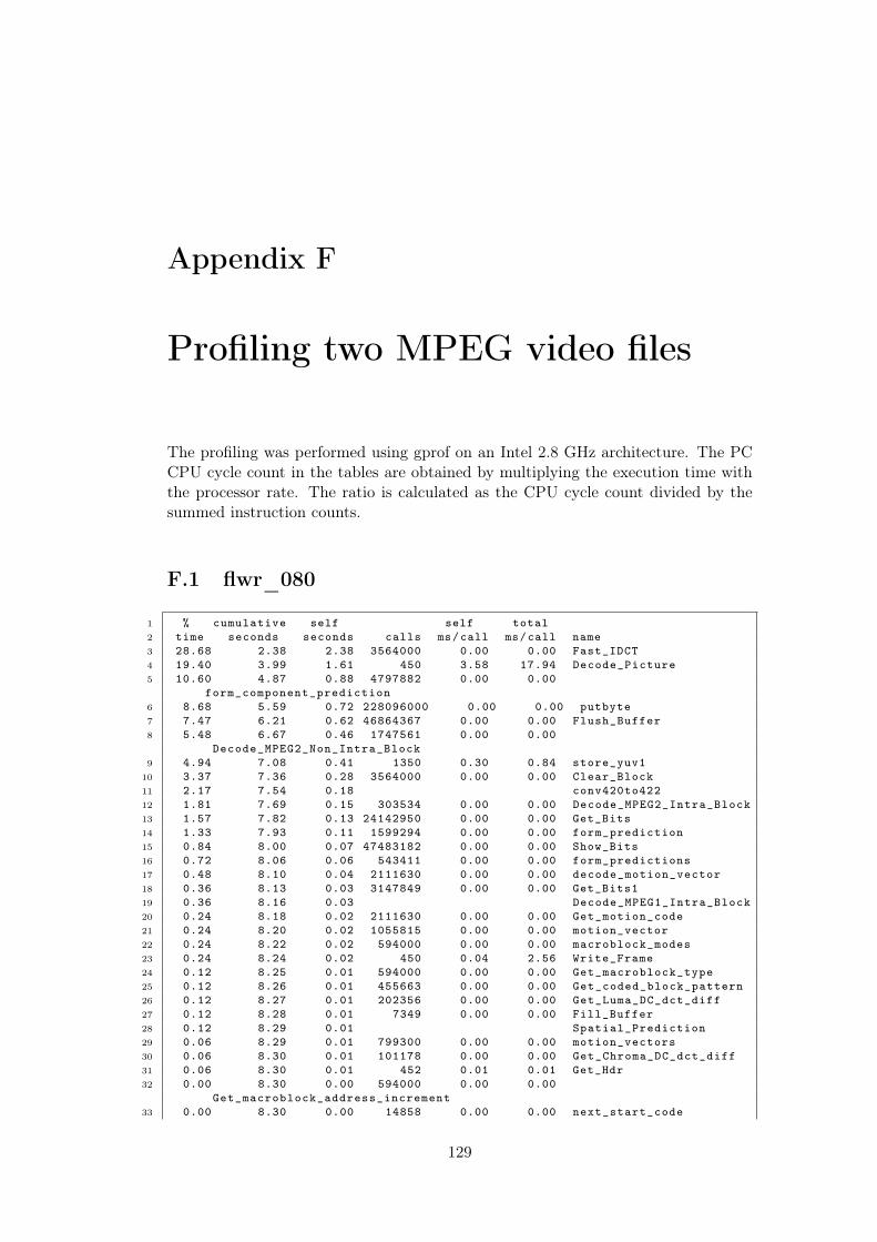
Appendix F
Profiling two MPEG video files
The profiling was performed using gprof on an Intel 2.8 GHz architecture. The PCCPU cycle count in the tables are obtained by multiplying the execution time withthe processor rate. The ratio is calculated as the CPU cycle count divided by thesummed instruction counts.
F.1 flwr_080
1 % cumulative self self total2 time seconds seconds calls ms/call ms/call name3 28.68 2.38 2.38 3564000 0.00 0.00 Fast_IDCT4 19.40 3.99 1.61 450 3.58 17.94 Decode_Picture5 10.60 4.87 0.88 4797882 0.00 0.00
form_component_prediction6 8.68 5.59 0.72 228096000 0.00 0.00 putbyte7 7.47 6.21 0.62 46864367 0.00 0.00 Flush_Buffer8 5.48 6.67 0.46 1747561 0.00 0.00
Decode_MPEG2_Non_Intra_Block9 4.94 7.08 0.41 1350 0.30 0.84 store_yuv1
10 3.37 7.36 0.28 3564000 0.00 0.00 Clear_Block11 2.17 7.54 0.18 conv420to42212 1.81 7.69 0.15 303534 0.00 0.00 Decode_MPEG2_Intra_Block13 1.57 7.82 0.13 24142950 0.00 0.00 Get_Bits14 1.33 7.93 0.11 1599294 0.00 0.00 form_prediction15 0.84 8.00 0.07 47483182 0.00 0.00 Show_Bits16 0.72 8.06 0.06 543411 0.00 0.00 form_predictions17 0.48 8.10 0.04 2111630 0.00 0.00 decode_motion_vector18 0.36 8.13 0.03 3147849 0.00 0.00 Get_Bits119 0.36 8.16 0.03 Decode_MPEG1_Intra_Block20 0.24 8.18 0.02 2111630 0.00 0.00 Get_motion_code21 0.24 8.20 0.02 1055815 0.00 0.00 motion_vector22 0.24 8.22 0.02 594000 0.00 0.00 macroblock_modes23 0.24 8.24 0.02 450 0.04 2.56 Write_Frame24 0.12 8.25 0.01 594000 0.00 0.00 Get_macroblock_type25 0.12 8.26 0.01 455663 0.00 0.00 Get_coded_block_pattern26 0.12 8.27 0.01 202356 0.00 0.00 Get_Luma_DC_dct_diff27 0.12 8.28 0.01 7349 0.00 0.00 Fill_Buffer28 0.12 8.29 0.01 Spatial_Prediction29 0.06 8.29 0.01 799300 0.00 0.00 motion_vectors30 0.06 8.30 0.01 101178 0.00 0.00 Get_Chroma_DC_dct_diff31 0.06 8.30 0.01 452 0.01 0.01 Get_Hdr32 0.00 8.30 0.00 594000 0.00 0.00
Get_macroblock_address_increment33 0.00 8.30 0.00 14858 0.00 0.00 next_start_code
129

Appendix F. Profiling two MPEG video files
34 0.00 8.30 0.00 14405 0.00 0.00 Flush_Buffer3235 0.00 8.30 0.00 13500 0.00 0.00 slice_header36 0.00 8.30 0.00 454 0.00 0.00 Get_Bits3237 0.00 8.30 0.00 452 0.00 0.01 Headers38 0.00 8.30 0.00 452 0.00 0.00 extension_and_user_data39 0.00 8.30 0.00 450 0.00 0.00 extra_bit_information40 0.00 8.30 0.00 450 0.00 2.51 store_one41 0.00 8.30 0.00 3 0.00 0.00 Initialize_Buffer42 0.00 8.30 0.00 3 0.00 0.00 marker_bit43 0.00 8.30 0.00 1 0.00 0.00 Initialize_Fast_IDCT44 0.00 8.30 0.00 1 0.00 2.56
Output_Last_Frame_of_Sequence
Block Description valueVLD/IQ Sum instruction counts 4.52521e9
PC execution time 0.9sPC CPU cycles 2.52e9
Ratio 0.557IDCT/MP Sum instruction counts 6.94239e10
PC execution time 3.45sPC CPU cycles 9.66e9
Ratio 0.139
Table F.1: Summary of profiling calculations for flwr_080
F.2 high_25fps_320x240
1 % cumulative self self total2 time seconds seconds calls ms/call ms/call name3 32.64 0.94 0.94 718200 0.00 0.00 Fast_IDCT4 14.58 1.36 0.42 633492 0.00 0.00
Decode_MPEG2_Non_Intra_Block5 11.11 1.68 0.32 399 0.80 6.92 Decode_Picture6 10.77 1.99 0.31 22715738 0.00 0.00 Flush_Buffer7 7.64 2.21 0.22 666834 0.00 0.00
form_component_prediction8 4.86 2.35 0.14 45964800 0.00 0.00 putbyte9 3.47 2.45 0.10 1197 0.08 0.20 store_yuv1
10 3.13 2.54 0.09 conv420to42211 2.43 2.61 0.07 11020727 0.00 0.00 Get_Bits12 2.43 2.68 0.07 718200 0.00 0.00 Clear_Block13 2.08 2.74 0.06 22845348 0.00 0.00 Show_Bits14 1.39 2.78 0.04 222278 0.00 0.00 form_prediction15 1.04 2.81 0.03 51366 0.00 0.00 Decode_MPEG2_Intra_Block16 0.69 2.83 0.02 203584 0.00 0.00 Get_motion_code17 0.69 2.85 0.02 4236 0.00 0.00 Fill_Buffer18 0.69 2.87 0.02 Decode_MPEG1_Intra_Block19 0.35 2.88 0.01 445 0.02 0.02 extension_and_user_data20 0.00 2.88 0.00 312616 0.00 0.00 Get_Bits121 0.00 2.88 0.00 203584 0.00 0.00 decode_motion_vector22 0.00 2.88 0.00 119645 0.00 0.00
Get_macroblock_address_increment23 0.00 2.88 0.00 119645 0.00 0.00 Get_macroblock_type24 0.00 2.88 0.00 119645 0.00 0.00 macroblock_modes25 0.00 2.88 0.00 111139 0.00 0.00 form_predictions26 0.00 2.88 0.00 111030 0.00 0.00 Get_coded_block_pattern27 0.00 2.88 0.00 101792 0.00 0.00 motion_vector28 0.00 2.88 0.00 101792 0.00 0.00 motion_vectors29 0.00 2.88 0.00 34244 0.00 0.00 Get_Luma_DC_dct_diff30 0.00 2.88 0.00 17122 0.00 0.00 Get_Chroma_DC_dct_diff
130

F.2. high_25fps_320x240
31 0.00 2.88 0.00 7300 0.00 0.00 next_start_code32 0.00 2.88 0.00 6854 0.00 0.00 Flush_Buffer3233 0.00 2.88 0.00 5985 0.00 0.00 slice_header34 0.00 2.88 0.00 447 0.00 0.00 Get_Bits3235 0.00 2.88 0.00 401 0.00 0.03 Get_Hdr36 0.00 2.88 0.00 401 0.00 0.03 Headers37 0.00 2.88 0.00 399 0.00 0.60 Write_Frame38 0.00 2.88 0.00 399 0.00 0.00 extra_bit_information39 0.00 2.88 0.00 399 0.00 0.60 store_one40 0.00 2.88 0.00 69 0.00 0.00 marker_bit41 0.00 2.88 0.00 3 0.00 0.00 Initialize_Buffer42 0.00 2.88 0.00 1 0.00 0.00 Initialize_Fast_IDCT43 0.00 2.88 0.00 1 0.00 0.60
Output_Last_Frame_of_Sequence
Block Description valueVLD/IQ Sum instruction counts 1.79033e9
PC execution time 0.57sPC CPU cycles 1.596e9
Ratio 0.891IDCT/MP Sum instruction counts 1.37487e10
PC execution time 1.2sPC CPU cycles 3.36e9
Ratio 0.244
Table F.2: Summary of profiling calculations for high_25fps_320x240
131

Appendix F. Profiling two MPEG video files
132

Appendix G
CD-rom contents
133

Appendix G. CD-rom contents
134

Appendix H
Case Study plots
H.1 Variability in the MPEG video files
135

Appendix H. Case Study plots
Figure
H.1:
The
variabilityin
theAPE
1stream
:flw
r_080.m
2v
136

H.1. Variability in the MPEG video files
Fig
ure
H.2
:The
variability
intheAPE
2stream
:high_25fps_
320x480.m2v
137

Appendix H. Case Study plots
H.2 Case study 1
Figure H.3: Buffer backlog for TC1.0 with the slow processing elements. Time isplotted in ps along the 1. axis, and the number of macro blocks in the buffer is plottedalong the 2. axis.
Figure H.4: Idle response times for TC1.0 with the slow processing elements. Thetime in ps is plotted along the 1. axis, and the idle time in ps is plotted along the 2.axis.
138
H.2. Case study 1
Figure H.5: Buffer backlog for TC1.0 with the fast processing elements. Time isplotted in ps along the 1. axis, and the number of macro blocks in the buffer is plottedalong the 2. axis.
Figure H.6: Idle response times for TC1.0 with the fast processing elements. Thetime in ps is plotted along the 1. axis, and the idle time in ps is plotted along the 2.axis.
139

Appendix H. Case Study plots
Figure H.7: Buffer backlog for TC1.1 with the slow processing elements. Time isplotted in ps along the 1. axis, and the number of macro blocks in the buffer is plottedalong the 2. axis.
Figure H.8: Idle response times for TC1.1 with the slow processing elements. Thetime in ps is plotted along the 1. axis, and the idle time in ps is plotted along the 2.axis.
140

H.2. Case study 1
Figure H.9: Buffer backlog for TC1.1 with the fast processing elements. Time isplotted in ps along the 1. axis, and the number of macro blocks in the buffer is plottedalong the 2. axis.
Figure H.10: Idle response times for TC1.1 with the fast processing elements. Thetime in ps is plotted along the 1. axis, and the idle time in ps is plotted along the 2.axis.
141
Appendix H. Case Study plots
Figure H.11: Buffer backlog for TC1.2 with the slow processing elements. Time isplotted in ps along the 1. axis, and the number of macro blocks in the buffer is plottedalong the 2. axis.
Figure H.12: Idle response times for TC1.2 with the slow processing elements. Thetime in ps is plotted along the 1. axis, and the idle time in ps is plotted along the 2.axis.
142
H.2. Case study 1
Figure H.13: Buffer backlog for TC1.2 with the fast processing elements. Time isplotted in ps along the 1. axis, and the number of macro blocks in the buffer is plottedalong the 2. axis.
Figure H.14: Idle response times for TC1.2 with the fast processing elements. Thetime in ps is plotted along the 1. axis, and the idle time in ps is plotted along the 2.axis.
143

Appendix H. Case Study plots
Figure H.15: Buffer backlog for TC1.3 with the slow processing elements. Time isplotted in ps along the 1. axis, and the number of macro blocks in the buffer is plottedalong the 2. axis.
Figure H.16: Idle response times for TC1.3 with the slow processing elements. Thetime in ps is plotted along the 1. axis, and the idle time in ps is plotted along the 2.axis.
144

H.2. Case study 1
Figure H.17: Buffer backlog for TC1.3 with the fast processing elements. Time isplotted in ps along the 1. axis, and the number of macro blocks in the buffer is plottedalong the 2. axis.
Figure H.18: Idle response times for TC1.3 with the fast processing elements. Thetime in ps is plotted along the 1. axis, and the idle time in ps is plotted along the 2.axis.
145

Appendix H. Case Study plots
H.3 Case study 2
Figure H.19: Buffer backlog for TC2.0 with the slow processing elements. Time isplotted in ps along the 1. axis, and the number of macro blocks in the buffer is plottedalong the 2. axis.
Figure H.20: Idle response times for TC2.0 with the slow processing elements. Thetime in ps is plotted along the 1. axis, and the idle time in ps is plotted along the 2.axis.
146
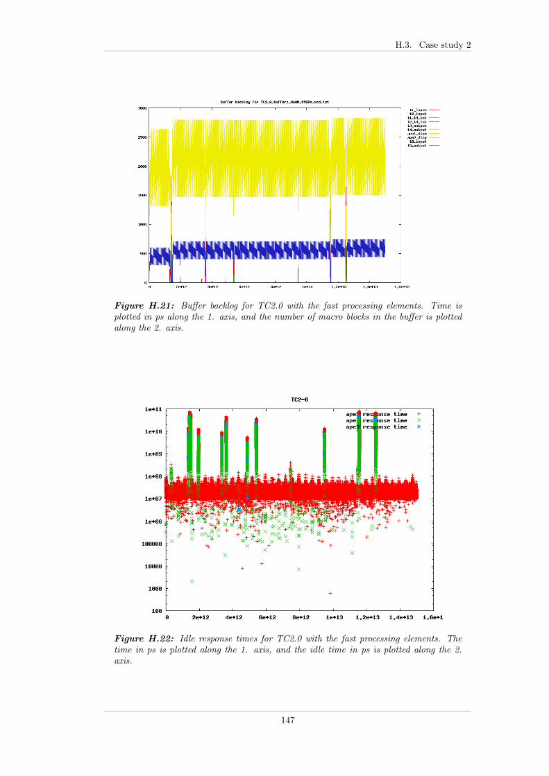
H.3. Case study 2
Figure H.21: Buffer backlog for TC2.0 with the fast processing elements. Time isplotted in ps along the 1. axis, and the number of macro blocks in the buffer is plottedalong the 2. axis.
Figure H.22: Idle response times for TC2.0 with the fast processing elements. Thetime in ps is plotted along the 1. axis, and the idle time in ps is plotted along the 2.axis.
147

Appendix H. Case Study plots
Figure H.23: Buffer backlog for TC2.1 with the slow processing elements. Time isplotted in ps along the 1. axis, and the number of macro blocks in the buffer is plottedalong the 2. axis.
Figure H.24: Idle response times for TC2.1 with the slow processing elements. Thetime in ps is plotted along the 1. axis, and the idle time in ps is plotted along the 2.axis.
148

H.3. Case study 2
Figure H.25: Buffer backlog for TC2.1 with the fast processing elements. Time isplotted in ps along the 1. axis, and the number of macro blocks in the buffer is plottedalong the 2. axis.
Figure H.26: Idle response times for TC2.1 with the fast processing elements. Thetime in ps is plotted along the 1. axis, and the idle time in ps is plotted along the 2.axis.
149

Appendix H. Case Study plots
Figure H.27: Buffer backlog for TC2.2 with the slow processing elements. Time isplotted in ps along the 1. axis, and the number of macro blocks in the buffer is plottedalong the 2. axis.
Figure H.28: Idle response times for TC2.2 with the slow processing elements. Thetime in ps is plotted along the 1. axis, and the idle time in ps is plotted along the 2.axis.
150

H.3. Case study 2
Figure H.29: Buffer backlog for TC2.2 with the fast processing elements. Time isplotted in ps along the 1. axis, and the number of macro blocks in the buffer is plottedalong the 2. axis.
Figure H.30: Idle response times for TC2.2 with the fast processing elements. Thetime in ps is plotted along the 1. axis, and the idle time in ps is plotted along the 2.axis.
151

Appendix H. Case Study plots
Figure H.31: Buffer backlog for TC2.3 with the slow processing elements. Time isplotted in ps along the 1. axis, and the number of macro blocks in the buffer is plottedalong the 2. axis.
Figure H.32: Idle response times for TC2.3 with the slow processing elements. Thetime in ps is plotted along the 1. axis, and the idle time in ps is plotted along the 2.axis.
152

H.3. Case study 2
Figure H.33: Buffer backlog for TC2.3 with the fast processing elements. Time isplotted in ps along the 1. axis, and the number of macro blocks in the buffer is plottedalong the 2. axis.
Figure H.34: Idle response times for TC2.3 with the fast processing elements. Thetime in ps is plotted along the 1. axis, and the idle time in ps is plotted along the 2.axis.
153
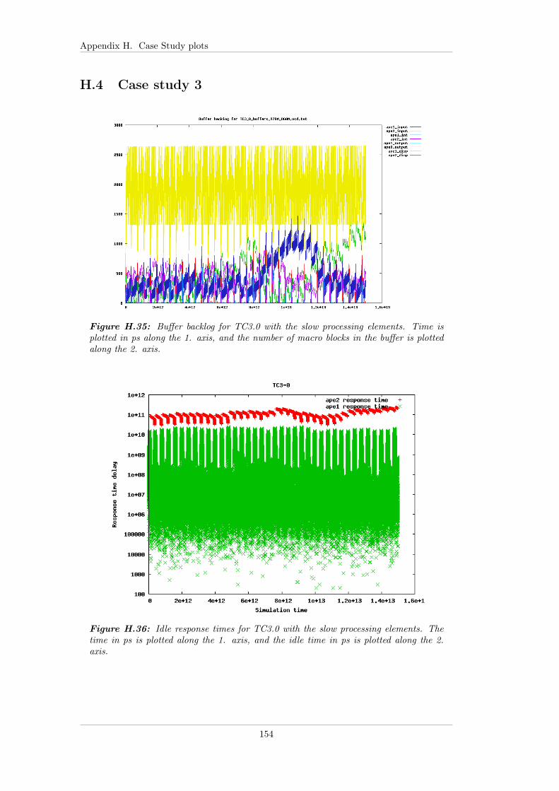
Appendix H. Case Study plots
H.4 Case study 3
Figure H.35: Buffer backlog for TC3.0 with the slow processing elements. Time isplotted in ps along the 1. axis, and the number of macro blocks in the buffer is plottedalong the 2. axis.
Figure H.36: Idle response times for TC3.0 with the slow processing elements. Thetime in ps is plotted along the 1. axis, and the idle time in ps is plotted along the 2.axis.
154

H.4. Case study 3
Figure H.37: Buffer backlog for TC3.0 with the fast processing elements. Time isplotted in ps along the 1. axis, and the number of macro blocks in the buffer is plottedalong the 2. axis.
Figure H.38: Idle response times for TC3.0 with the fast processing elements. Thetime in ps is plotted along the 1. axis, and the idle time in ps is plotted along the 2.axis.
155

Appendix H. Case Study plots
Figure H.39: Buffer backlog for TC3.1 with the slow processing elements. Time isplotted in ps along the 1. axis, and the number of macro blocks in the buffer is plottedalong the 2. axis.
Figure H.40: Idle response times for TC3.1 with the slow processing elements. Thetime in ps is plotted along the 1. axis, and the idle time in ps is plotted along the 2.axis.
156

H.4. Case study 3
Figure H.41: Buffer backlog for TC3.1 with the fast processing elements. Time isplotted in ps along the 1. axis, and the number of macro blocks in the buffer is plottedalong the 2. axis.
Figure H.42: Idle response times for TC3.1 with the fast processing elements. Thetime in ps is plotted along the 1. axis, and the idle time in ps is plotted along the 2.axis.
157

Appendix H. Case Study plots
Figure H.43: Buffer backlog for TC3.2 with the slow processing elements. Time isplotted in ps along the 1. axis, and the number of macro blocks in the buffer is plottedalong the 2. axis.
Figure H.44: Idle response times for TC3.2 with the slow processing elements. Thetime in ps is plotted along the 1. axis, and the idle time in ps is plotted along the 2.axis.
158

H.4. Case study 3
Figure H.45: Buffer backlog for TC3.2 with the fast processing elements. Time isplotted in ps along the 1. axis, and the number of macro blocks in the buffer is plottedalong the 2. axis.
Figure H.46: Idle response times for TC3.2 with the fast processing elements. Thetime in ps is plotted along the 1. axis, and the idle time in ps is plotted along the 2.axis.
159

Appendix H. Case Study plots
Figure H.47: Buffer backlog for TC3.3 with the slow processing elements. Time isplotted in ps along the 1. axis, and the number of macro blocks in the buffer is plottedalong the 2. axis.
Figure H.48: Idle response times for TC3.3 with the slow processing elements. Thetime in ps is plotted along the 1. axis, and the idle time in ps is plotted along the 2.axis.
160

H.4. Case study 3
Figure H.49: Buffer backlog for TC3.3 with the fast processing elements. Time isplotted in ps along the 1. axis, and the number of macro blocks in the buffer is plottedalong the 2. axis.
Figure H.50: Idle response times for TC3.3 with the fast processing elements. Thetime in ps is plotted along the 1. axis, and the idle time in ps is plotted along the 2.axis.
161

Appendix H. Case Study plots
H.5 Case study 4
Figure H.51: Buffer backlog for TC4.0 with the slow processing elements. Time isplotted in ps along the 1. axis, and the number of macro blocks in the buffer is plottedalong the 2. axis.
Figure H.52: Idle response times for TC4.0 with the slow processing elements. Thetime in ps is plotted along the 1. axis, and the idle time in ps is plotted along the 2.axis.
162

H.5. Case study 4
Figure H.53: Buffer backlog for TC4.1 with the slow processing elements. Time isplotted in ps along the 1. axis, and the number of macro blocks in the buffer is plottedalong the 2. axis.
Figure H.54: Idle response times for TC4.1 with the slow processing elements. Thetime in ps is plotted along the 1. axis, and the idle time in ps is plotted along the 2.axis.
163

Appendix H. Case Study plots
Figure H.55: Buffer backlog for TC4.2 with the slow processing elements. Time isplotted in ps along the 1. axis, and the number of macro blocks in the buffer is plottedalong the 2. axis.
Figure H.56: Idle response times for TC4.2 with the slow processing elements. Thetime in ps is plotted along the 1. axis, and the idle time in ps is plotted along the 2.axis.
164

H.5. Case study 4
Figure H.57: Buffer backlog for TC4.3 with the slow processing elements. Time isplotted in ps along the 1. axis, and the number of macro blocks in the buffer is plottedalong the 2. axis.
Figure H.58: Idle response times for TC4.3 with the slow processing elements. Thetime in ps is plotted along the 1. axis, and the idle time in ps is plotted along the 2.axis.
165

Appendix H. Case Study plots
Figure H.59: Buffer backlog for TC4.4 with the slow processing elements. Time isplotted in ps along the 1. axis, and the number of macro blocks in the buffer is plottedalong the 2. axis.
Figure H.60: Idle response times for TC4.4 with the slow processing elements. Thetime in ps is plotted along the 1. axis, and the idle time in ps is plotted along the 2.axis.
166

H.6. Case study 5
H.6 Case study 5
Figure H.61: Buffer backlog for TC5.0 with the slow processing elements. Time isplotted in ps along the 1. axis, and the number of macro blocks in the buffer is plottedalong the 2. axis.
Figure H.62: Idle response times for TC5.0 with the slow processing elements. Thetime in ps is plotted along the 1. axis, and the idle time in ps is plotted along the 2.axis.
167

Appendix H. Case Study plots
Figure H.63: Buffer backlog for TC5.0 with the fast processing elements. Time isplotted in ps along the 1. axis, and the number of macro blocks in the buffer is plottedalong the 2. axis.
Figure H.64: Idle response times for TC5.0 with the fast processing elements. Thetime in ps is plotted along the 1. axis, and the idle time in ps is plotted along the 2.axis.
168

H.6. Case study 5
Figure H.65: Buffer backlog for TC5.1 with the slow processing elements. Time isplotted in ps along the 1. axis, and the number of macro blocks in the buffer is plottedalong the 2. axis.
Figure H.66: Idle response times for TC5.1 with the slow processing elements. Thetime in ps is plotted along the 1. axis, and the idle time in ps is plotted along the 2.axis.
169

Appendix H. Case Study plots
Figure H.67: Buffer backlog for TC5.1 with the fast processing elements. Time isplotted in ps along the 1. axis, and the number of macro blocks in the buffer is plottedalong the 2. axis.
Figure H.68: Idle response times for TC5.1 with the fast processing elements. Thetime in ps is plotted along the 1. axis, and the idle time in ps is plotted along the 2.axis.
170

H.6. Case study 5
Figure H.69: Buffer backlog for TC5.2 with the slow processing elements. Time isplotted in ps along the 1. axis, and the number of macro blocks in the buffer is plottedalong the 2. axis.
Figure H.70: Idle response times for TC5.2 with the slow processing elements. Thetime in ps is plotted along the 1. axis, and the idle time in ps is plotted along the 2.axis.
171

Appendix H. Case Study plots
Figure H.71: Buffer backlog for TC5.2 with the fast processing elements. Time isplotted in ps along the 1. axis, and the number of macro blocks in the buffer is plottedalong the 2. axis.
Figure H.72: Idle response times for TC5.2 with the fast processing elements. Thetime in ps is plotted along the 1. axis, and the idle time in ps is plotted along the 2.axis.
172

H.6. Case study 5
Figure H.73: Buffer backlog for TC5.3 with the slow processing elements. Time isplotted in ps along the 1. axis, and the number of macro blocks in the buffer is plottedalong the 2. axis.
Figure H.74: Idle response times for TC5.3 with the slow processing elements. Thetime in ps is plotted along the 1. axis, and the idle time in ps is plotted along the 2.axis.
173

Appendix H. Case Study plots
Figure H.75: Buffer backlog for TC5.3 with the fast processing elements. Time isplotted in ps along the 1. axis, and the number of macro blocks in the buffer is plottedalong the 2. axis.
Figure H.76: Idle response times for TC5.3 with the fast processing elements. Thetime in ps is plotted along the 1. axis, and the idle time in ps is plotted along the 2.axis.
174
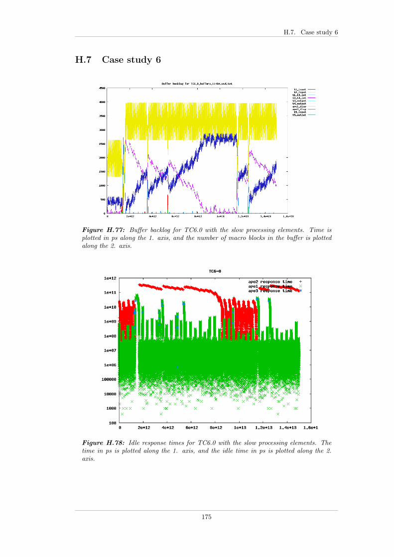
H.7. Case study 6
H.7 Case study 6
Figure H.77: Buffer backlog for TC6.0 with the slow processing elements. Time isplotted in ps along the 1. axis, and the number of macro blocks in the buffer is plottedalong the 2. axis.
Figure H.78: Idle response times for TC6.0 with the slow processing elements. Thetime in ps is plotted along the 1. axis, and the idle time in ps is plotted along the 2.axis.
175

Appendix H. Case Study plots
Figure H.79: Buffer backlog for TC6.0 with the fast processing elements. Time isplotted in ps along the 1. axis, and the number of macro blocks in the buffer is plottedalong the 2. axis.
Figure H.80: Idle response times for TC6.0 with the fast processing elements. Thetime in ps is plotted along the 1. axis, and the idle time in ps is plotted along the 2.axis.
176

H.7. Case study 6
Figure H.81: Buffer backlog for TC6.1 with the slow processing elements. Time isplotted in ps along the 1. axis, and the number of macro blocks in the buffer is plottedalong the 2. axis.
Figure H.82: Idle response times for TC6.1 with the slow processing elements. Thetime in ps is plotted along the 1. axis, and the idle time in ps is plotted along the 2.axis.
177

Appendix H. Case Study plots
Figure H.83: Buffer backlog for TC6.1 with the fast processing elements. Time isplotted in ps along the 1. axis, and the number of macro blocks in the buffer is plottedalong the 2. axis.
Figure H.84: Idle response times for TC6.1 with the fast processing elements. Thetime in ps is plotted along the 1. axis, and the idle time in ps is plotted along the 2.axis.
178

H.7. Case study 6
Figure H.85: Buffer backlog for TC6.2 with the slow processing elements. Time isplotted in ps along the 1. axis, and the number of macro blocks in the buffer is plottedalong the 2. axis.
Figure H.86: Idle response times for TC6.2 with the slow processing elements. Thetime in ps is plotted along the 1. axis, and the idle time in ps is plotted along the 2.axis.
179

Appendix H. Case Study plots
Figure H.87: Buffer backlog for TC6.2 with the fast processing elements. Time isplotted in ps along the 1. axis, and the number of macro blocks in the buffer is plottedalong the 2. axis.
Figure H.88: Idle response times for TC6.2 with the fast processing elements. Thetime in ps is plotted along the 1. axis, and the idle time in ps is plotted along the 2.axis.
180
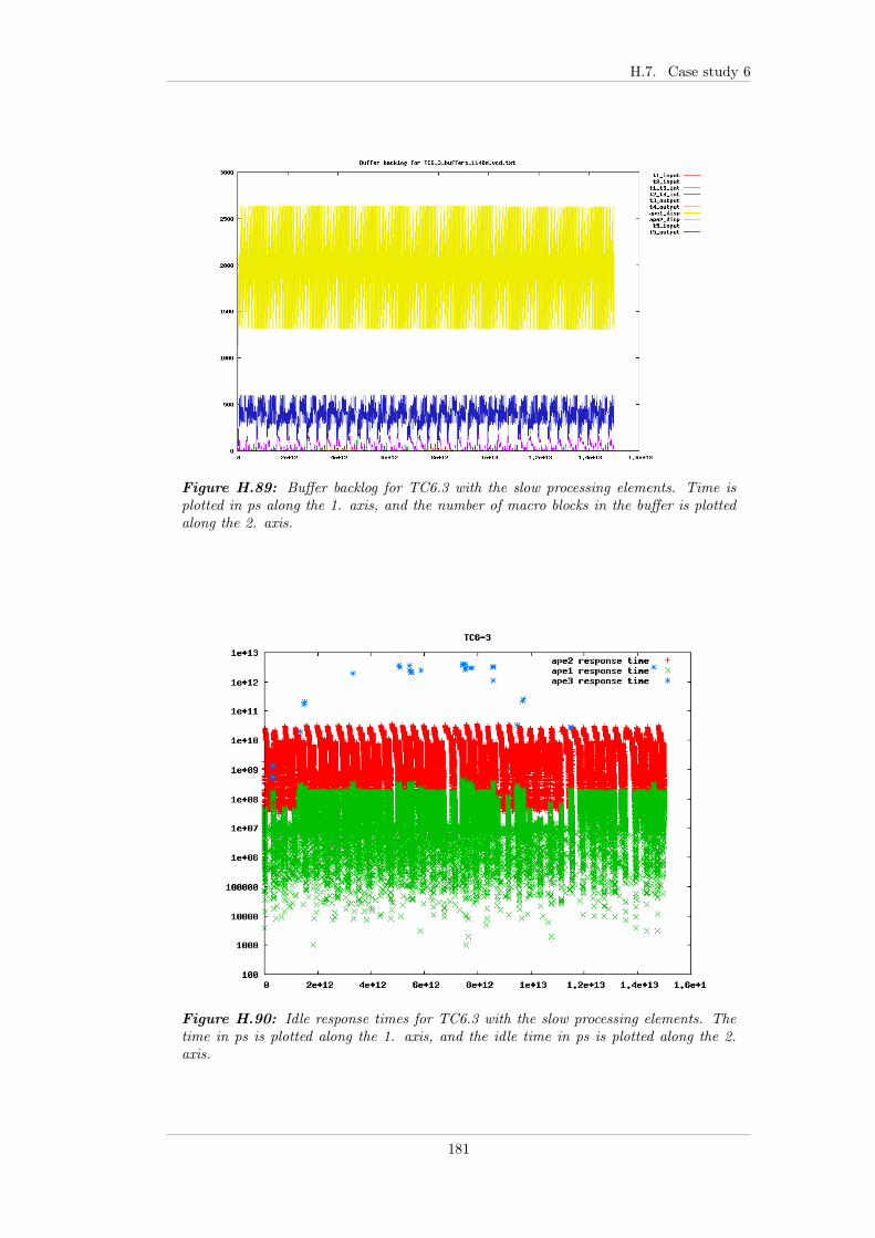
H.7. Case study 6
Figure H.89: Buffer backlog for TC6.3 with the slow processing elements. Time isplotted in ps along the 1. axis, and the number of macro blocks in the buffer is plottedalong the 2. axis.
Figure H.90: Idle response times for TC6.3 with the slow processing elements. Thetime in ps is plotted along the 1. axis, and the idle time in ps is plotted along the 2.axis.
181

Appendix H. Case Study plots
Figure H.91: Buffer backlog for TC6.3 with the fast processing elements. Time isplotted in ps along the 1. axis, and the number of macro blocks in the buffer is plottedalong the 2. axis.
Figure H.92: Idle response times for TC6.3 with the fast processing elements. Thetime in ps is plotted along the 1. axis, and the idle time in ps is plotted along the 2.axis.
182

H.8. Case study 7
H.8 Case study 7
Figure H.93: Buffer backlog for TC7.0 with the slow processing elements. Time isplotted in ps along the 1. axis, and the number of macro blocks in the buffer is plottedalong the 2. axis.
Figure H.94: Idle response times for TC7.0 with the slow processing elements. Thetime in ps is plotted along the 1. axis, and the idle time in ps is plotted along the 2.axis.
183
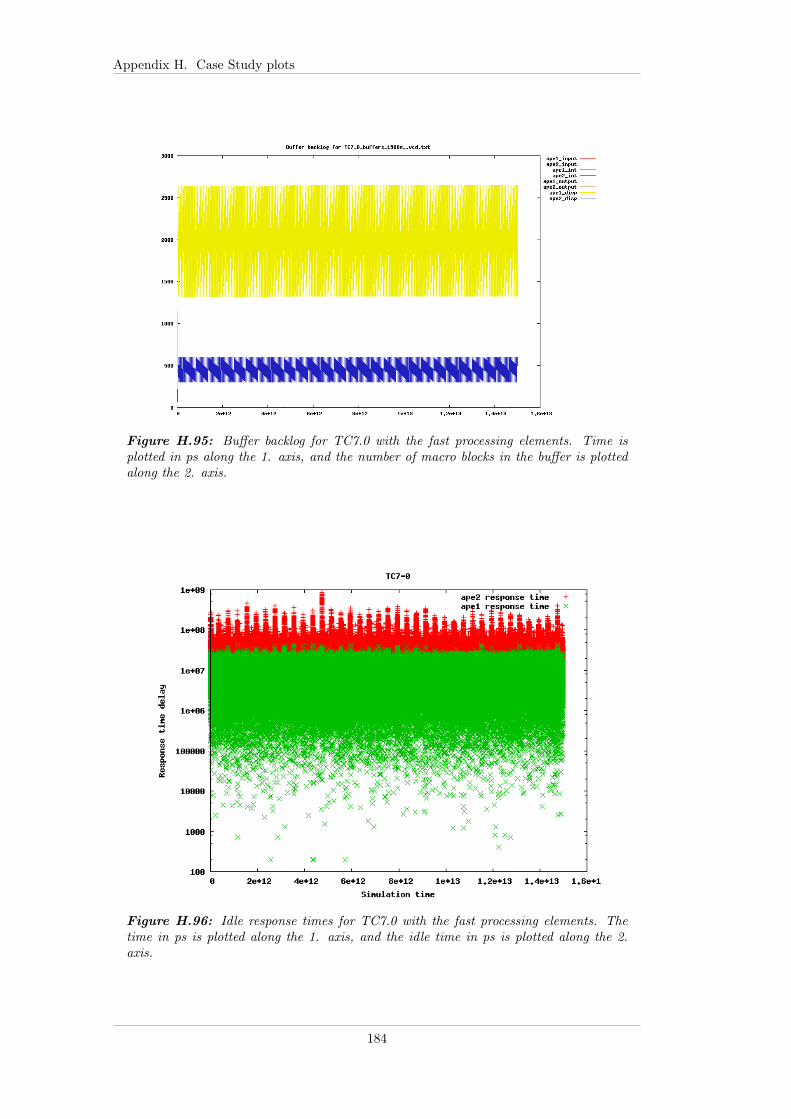
Appendix H. Case Study plots
Figure H.95: Buffer backlog for TC7.0 with the fast processing elements. Time isplotted in ps along the 1. axis, and the number of macro blocks in the buffer is plottedalong the 2. axis.
Figure H.96: Idle response times for TC7.0 with the fast processing elements. Thetime in ps is plotted along the 1. axis, and the idle time in ps is plotted along the 2.axis.
184
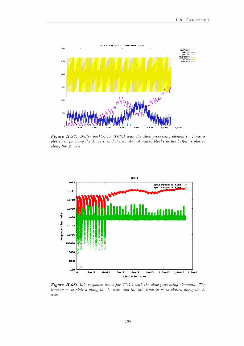
H.8. Case study 7
Figure H.97: Buffer backlog for TC7.1 with the slow processing elements. Time isplotted in ps along the 1. axis, and the number of macro blocks in the buffer is plottedalong the 2. axis.
Figure H.98: Idle response times for TC7.1 with the slow processing elements. Thetime in ps is plotted along the 1. axis, and the idle time in ps is plotted along the 2.axis.
185

Appendix H. Case Study plots
Figure H.99: Buffer backlog for TC7.1 with the fast processing elements. Time isplotted in ps along the 1. axis, and the number of macro blocks in the buffer is plottedalong the 2. axis.
Figure H.100: Idle response times for TC7.1 with the fast processing elements. Thetime in ps is plotted along the 1. axis, and the idle time in ps is plotted along the 2.axis.
186

H.8. Case study 7
Figure H.101: Buffer backlog for TC7.2 with the slow processing elements. Time isplotted in ps along the 1. axis, and the number of macro blocks in the buffer is plottedalong the 2. axis.
Figure H.102: Idle response times for TC7.2 with the slow processing elements. Thetime in ps is plotted along the 1. axis, and the idle time in ps is plotted along the 2.axis.
187

Appendix H. Case Study plots
Figure H.103: Buffer backlog for TC7.2 with the fast processing elements. Time isplotted in ps along the 1. axis, and the number of macro blocks in the buffer is plottedalong the 2. axis.
Figure H.104: Idle response times for TC7.2 with the fast processing elements. Thetime in ps is plotted along the 1. axis, and the idle time in ps is plotted along the 2.axis.
188

H.8. Case study 7
Figure H.105: Buffer backlog for TC7.3 with the slow processing elements. Time isplotted in ps along the 1. axis, and the number of macro blocks in the buffer is plottedalong the 2. axis.
Figure H.106: Idle response times for TC7.3 with the slow processing elements. Thetime in ps is plotted along the 1. axis, and the idle time in ps is plotted along the 2.axis.
189

Appendix H. Case Study plots
Figure H.107: Buffer backlog for TC7.3 with the fast processing elements. Time isplotted in ps along the 1. axis, and the number of macro blocks in the buffer is plottedalong the 2. axis.
Figure H.108: Idle response times for TC7.3 with the fast processing elements. Thetime in ps is plotted along the 1. axis, and the idle time in ps is plotted along the 2.axis.
190

H.9. Case study 8
H.9 Case study 8
Figure H.109: Buffer backlog for TC8.0 with the slow processing elements. Time isplotted in ps along the 1. axis, and the number of macro blocks in the buffer is plottedalong the 2. axis.
Figure H.110: Idle response times for TC8.0 with the slow processing elements. Thetime in ps is plotted along the 1. axis, and the idle time in ps is plotted along the 2.axis.
191
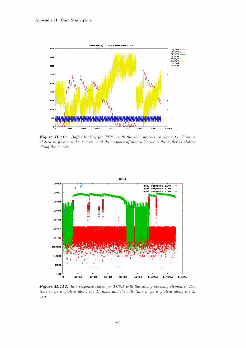
Appendix H. Case Study plots
Figure H.111: Buffer backlog for TC8.1 with the slow processing elements. Time isplotted in ps along the 1. axis, and the number of macro blocks in the buffer is plottedalong the 2. axis.
Figure H.112: Idle response times for TC8.1 with the slow processing elements. Thetime in ps is plotted along the 1. axis, and the idle time in ps is plotted along the 2.axis.
192

H.9. Case study 8
Figure H.113: Buffer backlog for TC8.2 with the slow processing elements. Time isplotted in ps along the 1. axis, and the number of macro blocks in the buffer is plottedalong the 2. axis.
Figure H.114: Idle response times for TC8.2 with the slow processing elements. Thetime in ps is plotted along the 1. axis, and the idle time in ps is plotted along the 2.axis.
193

Appendix H. Case Study plots
Figure H.115: Buffer backlog for TC8.3 with the slow processing elements. Time isplotted in ps along the 1. axis, and the number of macro blocks in the buffer is plottedalong the 2. axis.
Figure H.116: Idle response times for TC8.3 with the slow processing elements. Thetime in ps is plotted along the 1. axis, and the idle time in ps is plotted along the 2.axis.
194

H.9. Case study 8
Figure H.117: Buffer backlog for TC8.4 with the slow processing elements. Time isplotted in ps along the 1. axis, and the number of macro blocks in the buffer is plottedalong the 2. axis.
Figure H.118: Idle response times for TC8.4 with the slow processing elements. Thetime in ps is plotted along the 1. axis, and the idle time in ps is plotted along the 2.axis.
195

Appendix H. Case Study plots
Figure H.119: Buffer backlog for TC8.5 with the slow processing elements. Time isplotted in ps along the 1. axis, and the number of macro blocks in the buffer is plottedalong the 2. axis.
Figure H.120: Idle response times for TC8.5 with the slow processing elements. Thetime in ps is plotted along the 1. axis, and the idle time in ps is plotted along the 2.axis.
196

H.10. APE3 histogram
H.10 APE3 histogram
Figure H.121: Histogram of the processor cycles required for the APE3 stream (GUI).Most of the below task request require below 20.000 cycles, but some require up to40.000.000 cycles.
197