Implementation of a Symbolic Circuit Simulator forTopological Network Analysis*

Weiwei Chen and Guoyong ShiSchool of Microelectronics

Shanghai Jiao Tong UniversityShanghai 200030, China

{chenweiwei, shiguoyong}@ic. sj tu. edu. cn

Abstract- Many topological approaches to symbolic network analysishave been proposed in the literature, but none are implemented ultimatelyas a simulator for large network analysis due to their complexity andexponentially increasing number of terms. A novel methodology adoptedin this paper uses a graph reduction approach based on a set ofgraph reduction rules developed recently. Furthermore, a Binary DecisionDiagram is used in the implementation of a symbolic simulator that iscapable of analyzing large analog circuit blocks. Implementation detailsand experimental results are reported.Keywords-admissible term, BDD, graph reduction, symbolic

analysis

I. INTRODUCTION

Symbolic network analysis is a formal technique to calculate thebehavior or the characteristics of a circuit in terms of symbolicparameters. In contrast to numerical simulators such as SPICE [11],symbolic simulators can provide insights to the circuit behavior,showing performance trade-offs and sensitivities to parameter vari-ation and offering advantages in optimal topology selection, designspace exploration and fault detection [1]. Symbolic network analysisfrom topological perspective has been studied extensively in theliterature in the early 1950's [2], [3], [4] and recently [9]. One canfind a comprehensive review on this approach in the textbook [5].

Despite the intensive research in the past decades on symbolicnetwork analysis, most results did not come into practical simulators.The main difficulty arises from the exponential growth of the productterms with the number of nodes and elements in the circuit. A goodsymbolic simulator for exact analysis of large integrated circuit musthave efficient ways to generate and store the product terms.The simulator implemented in this paper is based on a graph

reduction algorithm developed recently [7], together with an efficientstorage scheme using Binary Decision Diagram (BDD) [6]. Witha good symbol ordering heuristic, the graph reduction process canbe represented by a BDD without exhausting the computer memoryand it is no longer needed to explicitly enumerate the exponentialnumber of terms. Furthermore, numerical analysis can be carried outefficiently due to the efficient implementation mechanism based onthe BDD.The work of this paper and [7] is based on the earlier work of [9]

where a valid tree pair idea was proposed, but without a fully devel-oped theory and a working implementation. This key contribution ofthis paper is on the implementation techniques based on an innovativegraph reduction idea. The graph reduction algorithms are introducedin Section II. Implementation details on the symbolic simulator arepresented in Section III. Experimental results are reported in SectionIV. Conclusion is made in Section V.

*This work was supported by the National Natural Science Foundation ofChina, Grant No. 60572028.

II. GRAPH REDUCTION ALGORITHMSA graph reduction algorithm is presented with an example in this

section. The circuits to be analyzed are allowed to contain elementssuch as impedances (Z), admittances (Y), four types of dependentsources (VCVS, CCCS, VCCS, CCVS), and independent source. Tosimplify formulation, the following assumptions are introduced:

Basic Assumptions. A controlling branch only controls one branch.. A controlled branch is controlled by only one branch.. There is only one independent source in the circuit under

analysis.The assumptions are not restrictive; complex circuits can be

remodeled to satisfy the assumptions in one way or another. For agiven circuit satisfying the basic assumptions, it can be converted to agraph according to the following rules (see Fig. 1 for an illustration.)

Graph Construction Rules(i) The edges associated with sources are directed, with voltage

(ii)

(iii)(iv)

edges from + to - and current edges along the current directionassigned.Add an edge for each controlling voltage. Each controllingcurrent takes a single edge.All edges are identified by their edge names.The input-output is modeled by an appropriate dependentsource.

R1 2~- 19 R 21c

Vs c 1 Vo C c

(a) (b)

Fig. 1. A circuit example.

S tadgG -pha

LFG 2 t oGraph Rt D-ph

Fig. 2. Construction of Graph Reduction Diagram.

1368

1-4244-0387-1/06/$20.00 ©g2006 IEEE

The graph construction rules basically assign a symbol to one

independent edge or a pair of two dependent edges. In our graphreduction approach, the input-output pair is always modeled as a

virtual dependent source, such as a VCVS (UO controls V, ) forthe example in Fig. l(b), with the corresponding symbol solvedsymbolically as the unknown.We continue to use the example in Fig. 1(a) to illustrate the

construction of a decision diagram based on a graph reductionprocess. Because of the presence of dependent sources, splitting thegraph into two subgraphs satisfying certain constraints would greatlysimplify the topological analysis. Fig. 2 shows the splitting of thegraph in Fig. l(b) into two subgraphs, called L-graph and R-graph.According to definition of admissible term given in the Appendix,the V, edge is only allowed in the R-graph.The L-graph and R-graph are then reduced edge-by-edge following

the Graph Reduction Algorithm until no further reduction is neces-

sary. We choose an order for the symbols to be manipulated, X < R< C, where symbol X is associated with the VCVS pair and X < Rmeans manipulating symbol X before symbol R. Each symbol hastwo operations in the graph reduction process, one for adding thissymbol into an admissible term (i.e., include the symbol) and theother for ignoring it (i.e., exclude the symbol). We begin with thesymbol X which refers to a VCVS pair associated with the input-output. At the beginning, the initial L-graph and R-graph are intact(see Fig. 3).The operations on the edges associated with different types of

symbols are summarized in Table I, which are derived from thedefinition of admissible terms (see the Appendix).

TABLE I

BINARY OPERATIONS FOR GRAPH REDUCTION

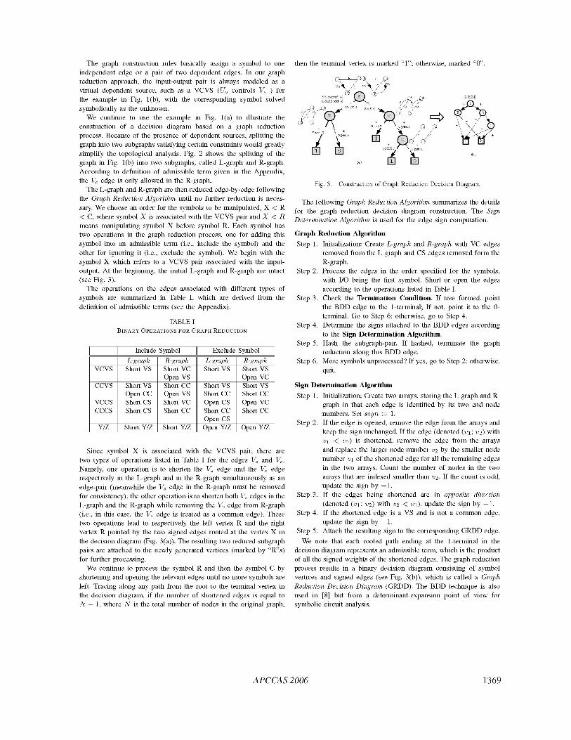
Since symbol X is associated with the VCVS pair, there are

two types of operations listed in Table I for the edges V, and Vc.Namely, one operation is to shorten the V, edge and the V, edgerespectively in the L-graph and in the R-graph simultaneously as an

edge-pair (meanwhile the V, edge in the R-graph must be removedfor consistency); the other operation is to shorten both V, edges in theL-graph and the R-graph while removing the VK edge from R-graph(i.e., in this case, the V, edge is treated as a common edge). Thesetwo operations lead to respectively the left vertex R and the rightvertex R pointed by the two signed edges rooted at the vertex X inthe decision diagram (Fig. 3(a)). The resulting two reduced subgraphpairs are attached to the newly generated vertices (marked by "R"s)for further processing.We continue to process the symbol R and then the symbol C by

shortening and opening the relevant edges until no more symbols are

left. Tracing along any path from the root to the terminal vertex inthe decision diagram, if the number of shortened edges is equal toN -1, where N is the total number of nodes in the original graph,

then the terminal vertex is marked "1"; otherwise, marked "O".

IXR(V ,V s) v s, V s) ., /C lc

ShortR OpenR (

I ~ ~ p I

(a) 1

=:> +P° +

/I\ +E2>'

Fig. 3. Construction of Graph Reduction Decision Diagram.

The following Graph Reduction Algorithm summarizes the detailsfor the graph reduction decision diagram construction. The SignDetermination Algorithm is used for the edge sign computation.

Graph Reduction AlgorithmStep 1. Initialization: Create L-graph and R-graph with VC edges

removed from the L-graph and CS edges removed form theR-graph.

Step 2. Process the edges in the order specified for the symbols,with I/O being the first symbol. Short or open the edgesaccording to the operations listed in Table 1.

Step 3. Check the Termination Condition. If tree formed, pointthe BDD edge to the 1-terminal; If not, point it to the 0-terminal. Go to Step 6; otherwise, go to Step 4.

Step 4. Determine the signs attached to the BDD edges accordingto the Sign Determination Algorithm.

Step 5. Hash the subgraph-pair. If hashed, terminate the graphreduction along this BDD edge.

Step 6. More symbols unprocessed? If yes, go to Step 2; otherwise,quit.

Sign Determination AlgorithmStep 1. Initialization: Create two arrays, storing the L-graph and R-

graph in that each edge is identified by its two end nodenumbers. Set sign := 1.

Step 2. If the edge is opened, remove the edge from the arrays andkeep the sign unchanged. If the edge (denoted (vi; V2) withVi < V2) is shortened, remove the edge from the arraysand replace the larger node number V2 by the smaller nodenumber vi of the shortened edge for all the remaining edgesin the two arrays. Count the number of nodes in the twoarrays that are indexed smaller than V2. If the count is odd,update the sign by -1.

Step 3. If the edges being shortened are in opposite direction(denoted (vi; V2) with V2 < vi), update the sign by -1.

Step 4. If the shortened edge is a VS and is not a common edge,update the sign by -1.

Step 5. Attach the resulting sign to the corresponding GRDD edge.We note that each rooted path ending at the 1-terminal in the

decision diagram represents an admissible term, which is the productof all the signed weights of the shortened edges. The graph reductionprocess results in a binary decision diagram consisting of symbolvertices and signed edges (see Fig. 3(b)), which is called a GraphReduction Decision Diagram (GRDD). The BDD technique is alsoused in [8] but from a determinant-expansion point of view forsymbolic circuit analysis.

APCCAS 2006

l_____ II Include Symbol if Exclude SymbolL-graph R-graph L-graph R-graph

VCVS Short VS Short VC Short VS Short VSOpenVS OpenVC

CCVS Short VS Short CC Short VS Short VSOpen CC Open VS Short CC Short CC

VCCS Short CS Short VC Open CS Open VCCCCS Short CS Short CC Short CC Short CCY/Z_ Short_Y/Z ShortY/Z Open CS

Y/Z Short Y/Z Short Y/Z Open Y/Z Open Y/Z

1369

In the graph reduction process, we shorten the edges by collapsingthe larger end node into the smaller one meanwhile relabel theremaining edge nodes that have been collapsed in the subgraphs.The node renumbering is needed for the determination of GRDDedge signs, which is based on a recursive processing of the incidencematrices of a subgraph pair.We refer the reader to [7] for a theoretical justification of the

algorithms listed in this section. The correctness of the algorithms isalso justified from implementation reported in the following sections.

III. SYMBOLIC SIMULATOR IMPLEMENTATION

Our symbolic simulator consists of a netlist parser, a symbolicanalysis engine (containing the GRDD) and a numerical analyzer.The netlist parser reads the standard SPICE netlist and converts itto a directed graph stored in the computer memory according to theGraph Construction Rules.The symbolic analysis engine processes the graph and constructs

a binary decision diagram in the computer memory, in which theunknown symbol X is at the root vertex. For the circuit in Fig. 1,the symbols are ordered as X > R > C and the GRDD constructedis shown in Fig. 3(b) with X being the virtual dependent pair(VCVS). The symbolic analysis engine generates the three productterms (rooted paths ending at the vertex 1) satisfying the homogenousequation (Theorem 1):

-X R-1 + R-1 + Cs = (1)

where X is the unknown. The transfer function from Vs to U0 is thenT(s) = IIX, where X is solved symbolically from (1) by sortingthe terms.

In the GRDD, all terms involving the X symbol are stored as the1-edge sub-diagram and those terms not involving the X symbol arestored as the 0-edge sub-diagram of the GRDD root. The analyzerevaluates the product terms stored in the GRDD with all symbolssubstituted by their (complex) numerical values (with the Z valuesinverted) and divides the value of 1-edge by that of the 0-edge atthe root to get the one-point frequency response. The analyzer alsocalculates the statistics of the decision diagram, including the numberof vertices created and the number of terms it represents, etc.The GRDD construction details have been articulated in the

previous section. Described below are the implementation details thatare critical for GRDD efficiency.

A. Symbol Ordering HeuristicThe symbol processing order strongly affects the size of GRDD.

In the current implementation, the symbols of the circuit elementsare ordered starting from the I/O port, then the elements directlyconnected to it, and then the elements connect to the previouslyordered elements until all of the symbols are ordered. This processof ordering is easily implemented in a breadth first fashion. Wedefine some priorities for those equivalent elements (elements thatare all connected to the previously ordered ones). The impedances(admittances) are assigned the higher priority but ordered at random.This ordering heuristic is from the consideration of early termination,namely, graph disconnectivity can be detected early. We believe otherbetter good orderings exist by exploring the circuit topology.

B. GRDD SharingAs usual, the efficiency of BDD implementation comes from the

sub-diagram sharing. In the same vein, the GRDD sharing is consid-ered in our implementation as well. The sub-GRDD sharing comesfrom the fact that in the graph-pair reduction process, some later

reduced graph-pairs will find themselves identical or topologicallyisomorphic to the earlier reduced graph-pairs.

In GRDD construction, we always merge two end nodes of an edgeby retaining the smaller node number. This convention would endup with certain reduced subgraphs (from different reduction paths)having the same topology but different node numberings. We callsuch reduced subgraphs isomorphic subgraphs (see Fig. 4(a) for anexample). Furthermore, as shown in Fig. 5, although the two subgraphpairs have different topologies, they lead to two identical sub-GRDDs.We call such reduced subgraphs term-equivalent subgraphs.

It is easy to observe that both isomorphic and term-equivalentsubgraphs would result in the same set of admissible sub-terms (seeFig. 4(b) and Fig. 5 for examples), regardless of the node numberingand even the subgraph topologies.

Subgraph isomorphism and term-equivalence could possibly leadto sub-GRDD sharing. In our implementation, identical subgraphpairs are shared first, followed by considering whether the associatedGRDD vertices can be shared. GRDD vertices are shared whentheir attached reduced subgraph pairs, symbol indexes and the signsattached to their incident edges are all identical to each other. Thetwo sharings are implemented by hash functions. The hash key forthe identical subgraph sharing is determined by the topology of thesubgraph pair, while the hash key for the vertex sharing is determinedby the attached reduced subgraph pair, symbol index and the signof the incident edge. Hash tables are used to keep each reducedsubgraph-pair and GRDD vertex unique.

Note that the vertex sharing implemented above did not considerthe possible sharing resulting from isomorphic and term-equivalence.For better efficiency, this part of vertex sharing is implementedin the second phase called GRDD reduction explained in the nextsubsection.

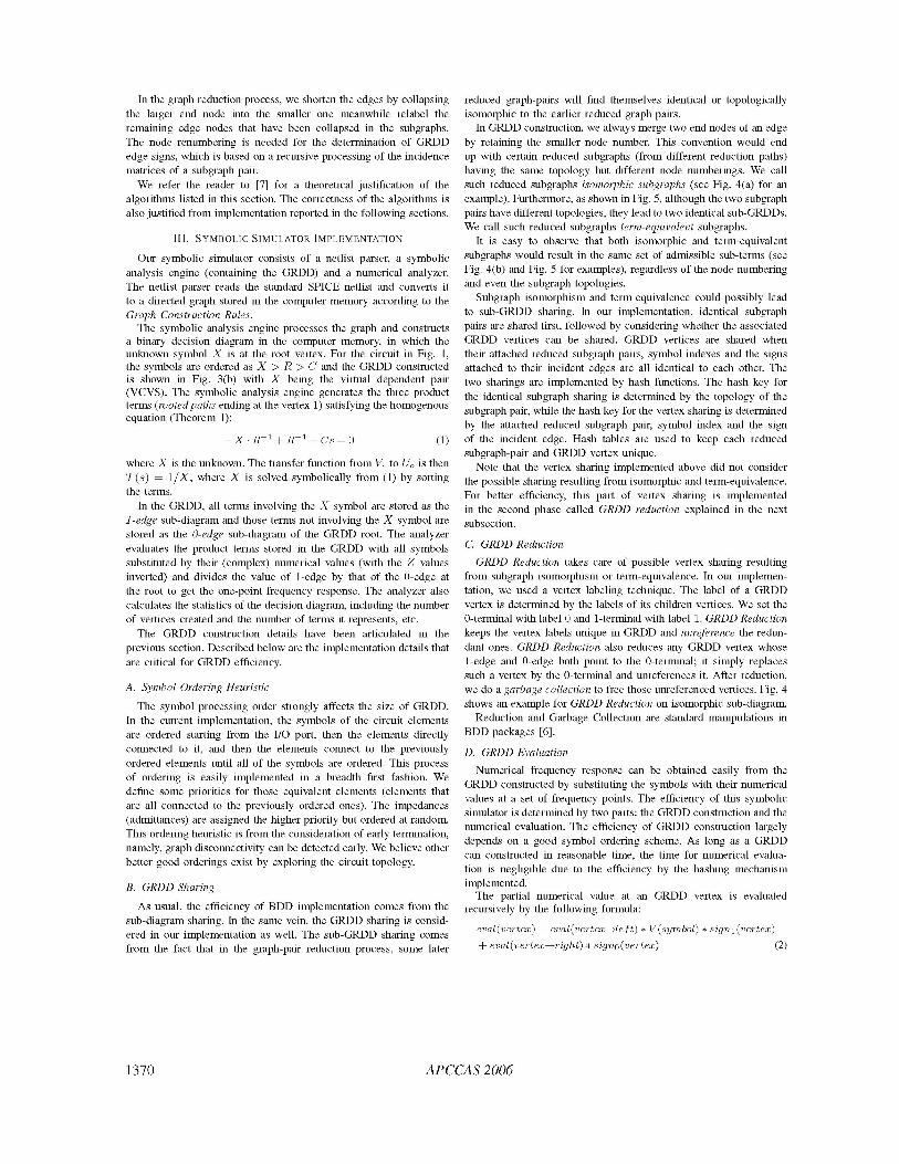
C. GRDD ReductionGRDD Reduction takes care of possible vertex sharing resulting

from subgraph isomorphism or term-equivalence. In our implemen-tation, we used a vertex labeling technique. The label of a GRDDvertex is determined by the labels of its children vertices. We set the0-terminal with label 0 and 1-terminal with label 1. GRDD Reductionkeeps the vertex labels unique in GRDD and unreference the redun-dant ones. GRDD Reduction also reduces any GRDD vertex whose1-edge and 0-edge both point to the 0-terminal; it simply replacessuch a vertex by the 0-terminal and unreferences it. After reduction,we do a garbage collection to free those unreferenced vertices. Fig. 4shows an example for GRDD Reduction on isomorphic sub-diagram.

Reduction and Garbage Collection are standard manipulations inBDD packages [6].

D. GRDD EvaluationNumerical frequency response can be obtained easily from the

GRDD constructed by substituting the symbols with their numericalvalues at a set of frequency points. The efficiency of this symbolicsimulator is determined by two parts: the GRDD construction and thenumerical evaluation. The efficiency of GRDD construction largelydepends on a good symbol ordering scheme. As long as a GRDDcan constructed in reasonable time, the time for numerical evalua-tion is negligible due to the efficiency by the hashing mechanismimplemented.

The partial numerical value at an GRDD vertex is evaluatedrecursively by the following formula:

eval(vertex) = eval(vertex-seft) * V(symbol) * signi(vertex)+ eval(vertex-sright) * signo(vertex) (2)

APCCAS 20061370

IV. EXPERIMENTAL RESULTS

----------------------------. r*., IF..... ... * .

*9 I"%)II____p-------------------------------,

/1/ -Op-C Sh-t OpeC Sh-tC S \ 1

GFRgDD BeeRoeductrn GRDD AiorReductn(c) GRDD Reduct:bn

Fig. 4. An example for GRDD reduction.

wabG RDbD1 ab-

Fig. 5. Identical sub-GRDDs generated by topologically different graph pairs.

where vertex is any GRDD vertex, eval(vertex) is the complexvalue calculated at vertex vertex, vertex-left points to the childvertex connected by the 1-edge and vertex--right points to the childvertex connected by the 0-edge, sign, and signo are respectivelythe signs attached to the 1-edge and 0-edge, and V(symbol) is thenumerical value of the symbol at the GRDD vertex (with the Zvalue inverted). With hashing techniques, the complexity of recursivenumerical evaluation is linear in the GRDD size.

E. Strategies for Efficiency1) Lumping parallel branches: The circuit to be analyzed usually

contain parallel elements that appear as parallel edges in the con-verted graph. Lumping these parallel branches to one branch meansmultiple symbols are combined into one symbol, by which the graphcomplexity and the number of product terms are reduced remarkably.

2) Early Disconnectivity Detection: Part of the Termination Con-dition in the GRDD Construction Algorithm is by detecting the graphdisconnectivity as early as possible. We count the number of the edgesin the reduced graph by counting those parallel edges as one edge andignoring those self-looped edges. If the number of edges is less thanthe number of the vertices of the reduced graph minus one, then thereduced graph is disconnected and the current GRDD vertex shouldbe pointed to the 0-terminal.

Our simulator was implemented in C++ and run on Intel Pentium1.73GHz processor with 1G memory. Three benchmark circuits usedin our experiment are:

,ua741, a bipolar opamp containing 24 transistors (same circuitused in [8], Fig. 15.),ua725, a bipolar opamp containing 26 transistors (same circuitused in [10], Fig. 13.)MOSopamp, a MOS cascode opamp containing 22 transistors(same circuit used in [10], Fig. 8.)

The small signal models for the MOSFET and bipolar transistors arethe same as that used in [8], Fig. 14, or in [10], Fig. 4.

Table II shows the simulator performance of the sample circuits.edge lump is the number of edges after the parallel elements arelumped. IGRDDI is the size of GRDD. Note that for the /ia725circuit we used a different ordering heuristic than the one describedbefore. A universally applicable ordering heuristic is still underinvestigation.

Table II also shows the effects of GRDD Sharing and GRDDReduction. The number of GRDD vertices is much less after GRDDreduction comparing to that before GRDD reduction. GRDD Sharinghappens frequently during the construction.Shown in Fig. 6 is a set of frequency responses produced by our

symbolic simulator and HSPICE. The results of our simulator matchexactly those obtained from HSPICE [12]. These results provides partof justification for the correctness of our symbolic simulator.The experimental results show that our symbolic simulator is

capable of generating the exact network functions of large analogcircuits, such as ,ua741 and ,ua725, in the scale of seconds. (Note thatin [10] the authors use approximate techniques to analyze ,ua725.)

ua741 Frequency Response100 200

hspice hspicegrdd 100 grdd

10 105 10 10° 101%frequency(Hz) frequency(Hz)

ua725 Frequency Response

10 10"' 10 10frequency(Hz) frequency(Hz)

Fig. 6. Frequency responses of the benchmark circuits (hspice vs. grdd).

APCCAS 2006

... ...

0

---------;--

1371

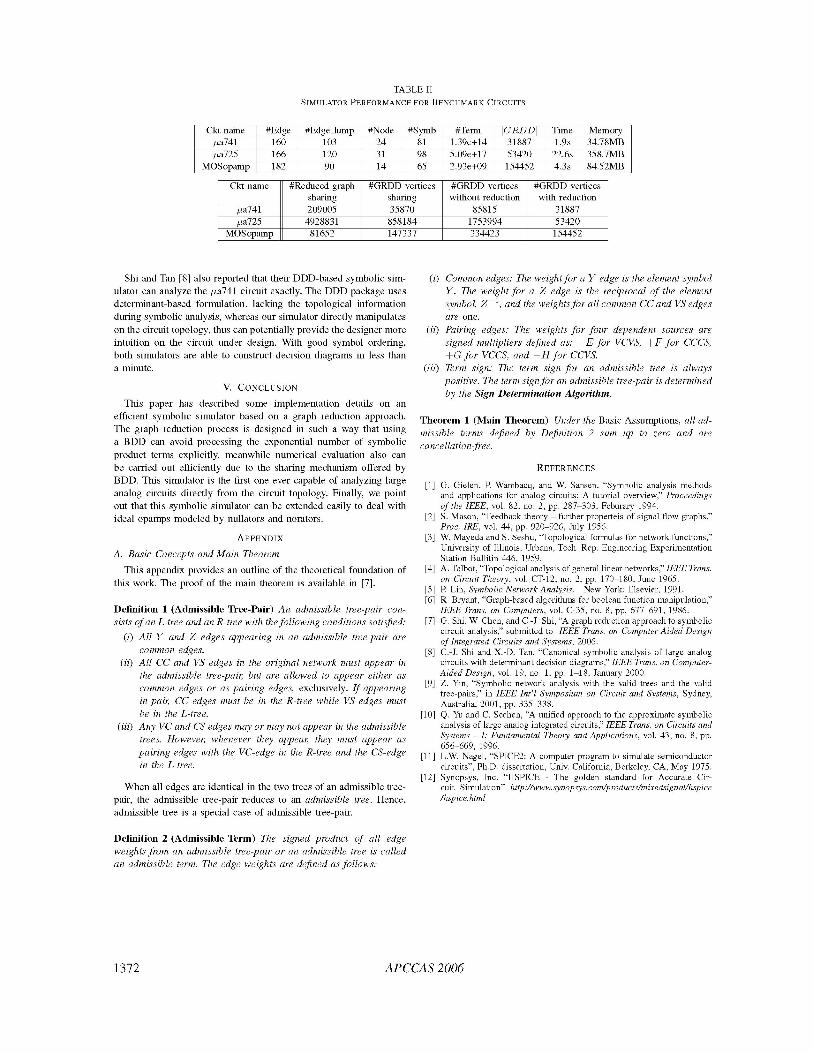
TABLE IISIMULATOR PERFORMANCE FOR BENCHMARK CIRCUITS

Cikt name

pta741pta725

MOSopamp

I#Edge160166182

#Edge-lump10312090 F

#Node #Symb24 8131 9814 65 F

#Tlerm1.39e+145.09e+172.93e+09

IGRDDI3188753420154452

Tlime1.9s22.6s4.3s

Memory34.78MB358.7MB84.52MB

Ckt name #Reduced graph #GRDD vertices #GRDD vertices #GRDD verticessharing sharing without reduction with reduction

pta741 209005 35870 85815 31887pia725 4928831 858184 1753994 53420

MOSopamp 81652 147337 334423 154452

Shi and Tan [8] also reported that their DDD-based symbolic sim-ulator can analyze the pta741 circuit exactly. The DDD package usesdetermiinant-based formulation, lacking the topological informationduring symbolic analysis, whereas our simulator directly manipulateson the circuit topology, thus can potentially provide the designer moreintuition on the circuit under design. With good symbol ordering,both simulators are able to construct decision diagrams in less thana minute.

V. CONCLUSIONThis paper has described some implementation details on an

efficient symbolic simulator based on a graph reduction approach.The graph reduction process is designed in such a way that usinga BDD can avoid processing the exponential number of symbolicproduct terms explicitly, meanwhile numerical evaluation also canbe carried out efficiently due to the sharing mechanism offered byBDD. This simulator is the first one ever capable of analyzing largeanalog circuits directly from the circuit topology. Finally, we pointout that this symbolic simulator can be extended easily to deal withideal opamps modeled by nullators and norators.

APPENDIXA. Basic Concepts and Main Theorem

This appendix provides an outline of the theoretical foundation ofthis work. The proof of the main theorem is available in [7].

Definition 1 (Admissible Tree-Pair) An admissible tree-pair con-sists ofan L-tree and an R-tree with the following conditions satisfied:

(i) All Y and Z edges appearing in an admissible tree-pair arecommon edges.

(ii) All CC and VS edges in the original network must appear inthe admissible tree-pair, but are allowed to appear either ascommon edges or as pairing edges, exclusively. If appearingin pair, CC edges must be in the R-tree while VS edges mustbe in the L-tree.

(iii) Any VC and CS edges may or may not appear in the admissibletrees. However, whenever they appear, they must appear aspairing edges with the VC-edge in the R-tree and the CS-edgein the L-tree.

When all edges are identical in the two trees of an admissible tree-pair, the admissible tree-pair reduces to an admissible tree. Hence,admiissible tree is a special case of admissible tree-pair.

(i) Common edges: The weightfor a Y edge is the element symbolY. The weight for a Z edge is the reciprocal of the elementsymbol, Z 1,and the weights for all common CC and VS edgesare one.

(ii) Pairing edges: The weights for four dependent sources aresigned multipliers defined as: FE for VCVS, -HF for CCCS,-HG for VCCS, and -H for CCVS.

(iii) Term sign: The term sign for an admissible tree is alwayspositive. The term signfor an admissible tree-pair is determinedby the Sign Determination Algorithm.

Theorem 1 (Main Theorem) Under the Basic Assumptions, all ad-missible terms defined by Definition 2 sum up to zero and arecancellation-free.

REFERENCES

[1] G. Gielen, P. Wambacq, and W. Sansen, "Symbolic analysis methodsand applications for analog circuits: A tutorial overview," Proceedingsof the IEEE, vol. 82, no. 2, pp. 287 303, Feburary 1994.

[2] 5. Mason, "Feedback theory -further properteis of signal flow graphs,"Proc. IRE, vol. 44, pp. 920 926, July 1956.

[3] W. Mayeda and S. Seshu, "Topological formulas for network functions,"University of Illinois, Urbana, Tech. Rep. Engineering ExperimentationStation Bullitin 446, 1959.

[4] A. Talbot, "Topological analysis of general linear networks," IEEE Trans.on Circuit Theory, vol. CT 12, no. 2, pp. 170 180, June 1965.

[5] P. Lin, Symbolic Network Analysis. New York: Elsevier, 1991.[6] R. Bryant, "Graph-based algorithms for boolean function manipulation,"

IEEE Trans. on Computers, vol. C-35, no. 8, pp. 677-691, 1986.[7] G. Shi, W. Chen, and C.-J. Shi, "A graph reduction approach to symbolic

circuit analysis," submitted to IEEE Trans. on Computer-Aided Designof Integrated Circuits and Systems, 2006.

[8] C.-J. Shi and X.-D. Tan, "Canonical symbolic analysis of large analogcircuits with determinant decision diagrams," IEEE Trans. on Computer-Aided Design, vol. 19, no. 1, pp. 1-18, January 2000.

[9] Z. Yin, "Symbolic network analysis with the valid trees and the validtree-pairs," in IEEE Int'l Symposium on Circuit and Systems, Sydney,Australia, 2001, pp. 335-338.

[10] Q. Yu and C. Sechen, "A unified approach to the approximate symbolicanalysis of large analog integrated circuits," IEEE Trans. on Circuits andSystems I:- Fundamental Theory and Applications, vol. 43, no. 8, pp.656-669, 1996.

[11] L.W. Nagel, "SPICE2: A computer program to simulate semiconductorcircuits", Ph.D. dissertation, Univ. California, Berkeley, CA, May 1975.

[12] Synopsys, Inc. "HSPICE- The golden standard for Accurate Cir-cuit Simulation" htp-lwsnpy.oiprdcsmxdinlhpc/hspice.html

Definition 2 (Admissible Term) The signed product of all edgeweights from an admissible tree-pair or an admissible tree is calledan admissible term. The edge weights are defined as follows:

1372 ~~~~~~~APCCAS 2006

- 11- . 11- . 11 I 11 - 11- - - - -

I

i

1372