definition, implementation, and calibration of ... -...
TRANSCRIPT

Definition, Implementation, and Calibration of theSwarmbot3D Simulator
Giovanni C. [email protected]
Ivo W. [email protected]
Luca M. [email protected]
Technical Report No. IDSIA-21-03December 16, 2003
IDSIA / USI-SUPSI*
Instituto Dalle Molle di studi sull’ intelligenza artificialeGalleria 2CH-6900 Manno, Switzerland
* IDSIA was founded by the Fondazione Dalle Molle per la Qualita della Vita and is affiliated with both the Universita della Svizzera italiana (USI)and the Scuola unversitaria professionale della Svizzera italiana (SUPSI) in Lugano. This research is funded by European Union and the SwissGovernment under grant 01.0012

Definition, Implementation, and Calibration of theSwarmbot3D Simulator
Giovanni C. [email protected]
Ivo W. [email protected]
Luca M. [email protected]
December 16, 2003

Abstract
This Technical Report describes the final version of the simulating software Swarmbot3d implementing theswarm-bot simulator as outlined in Workpackage 3, ”Simulator Prototype”.
The document presents all the simulator’s features and acts as a developer’s manual. It describes theimplementation choices and software components. It is complemented with the simulator software in itsfinal version, and the Simulator User Manual for its quick use. The simulator presented here is basedon the hardware specifications described in Deliverable 3 (”Simulator Design”) and Deliverable 5 (”UserManual”) of Workpackage 3 of the SWARMBOTS Project.
The development of the simulator Swarmbot3d was intended to address the following supporting rolesduring this project:
1. To be able to predict accurately both kinematics and dynamics of a single s-bot and swarm-bot in3D;
2. To evaluate hardware design options for different components;
3. To design swarm-bot experiments in 3D worlds; and
4. To investigate different distributed control algorithms.

Contents
1 Introduction 31.1 Simulator Taxonomy . . . . . . . . . . . . . . . . . . . . . . . . . . . . . . . . . . . . . 31.2 Survey of Existing Simulator Software . . . . . . . . . . . . . . . . . . . . . . . . . . . . 41.3 Characteristics of Swarmbot3d . . . . . . . . . . . . . . . . . . . . . . . . . . . . . . . . 71.4 Development Notes . . . . . . . . . . . . . . . . . . . . . . . . . . . . . . . . . . . . . . 71.5 Presentation of Published Work on Swarmbot3d . . . . . . . . . . . . . . . . . . . . . . . 8
2 Modeling and Design 92.1 Simulator Design . . . . . . . . . . . . . . . . . . . . . . . . . . . . . . . . . . . . . . . 9
2.1.1 Modular design . . . . . . . . . . . . . . . . . . . . . . . . . . . . . . . . . . . . 92.1.2 Multi-level modeling . . . . . . . . . . . . . . . . . . . . . . . . . . . . . . . . . 92.1.3 Dynamic model exchange . . . . . . . . . . . . . . . . . . . . . . . . . . . . . . 10
2.2 S-Bot Modeling . . . . . . . . . . . . . . . . . . . . . . . . . . . . . . . . . . . . . . . . 102.2.1 Treels Module . . . . . . . . . . . . . . . . . . . . . . . . . . . . . . . . . . . . 122.2.2 Turret Module . . . . . . . . . . . . . . . . . . . . . . . . . . . . . . . . . . . . 162.2.3 Front Gripper Module . . . . . . . . . . . . . . . . . . . . . . . . . . . . . . . . 182.2.4 Flexible Side Arm Module . . . . . . . . . . . . . . . . . . . . . . . . . . . . . . 222.2.5 Camera Module . . . . . . . . . . . . . . . . . . . . . . . . . . . . . . . . . . . . 242.2.6 Proximity Sensor Module . . . . . . . . . . . . . . . . . . . . . . . . . . . . . . 262.2.7 Ground IR Sensor Module . . . . . . . . . . . . . . . . . . . . . . . . . . . . . . 292.2.8 Light Ring Module . . . . . . . . . . . . . . . . . . . . . . . . . . . . . . . . . . 312.2.9 Inclinometer Module . . . . . . . . . . . . . . . . . . . . . . . . . . . . . . . . . 342.2.10 Sound Module . . . . . . . . . . . . . . . . . . . . . . . . . . . . . . . . . . . . 352.2.11 Temperature and Humidity Sensors Module . . . . . . . . . . . . . . . . . . . . . 382.2.12 Battery Voltage Meter Module . . . . . . . . . . . . . . . . . . . . . . . . . . . . 39
2.3 Swarm Modeling . . . . . . . . . . . . . . . . . . . . . . . . . . . . . . . . . . . . . . . 402.4 Environment Modeling . . . . . . . . . . . . . . . . . . . . . . . . . . . . . . . . . . . . 42
2.4.1 Terrain Modeling . . . . . . . . . . . . . . . . . . . . . . . . . . . . . . . . . . . 422.4.2 Light and light sensors . . . . . . . . . . . . . . . . . . . . . . . . . . . . . . . . 44
3 Reference Models 463.1 Fast Model . . . . . . . . . . . . . . . . . . . . . . . . . . . . . . . . . . . . . . . . . . 463.2 Simple Model . . . . . . . . . . . . . . . . . . . . . . . . . . . . . . . . . . . . . . . . . 463.3 Medium Model . . . . . . . . . . . . . . . . . . . . . . . . . . . . . . . . . . . . . . . . 473.4 Detailed Model . . . . . . . . . . . . . . . . . . . . . . . . . . . . . . . . . . . . . . . . 48
1

Technical Report No. IDSIA-21-03 2
4 Validation Experiments 514.1 Validation Against Hardware . . . . . . . . . . . . . . . . . . . . . . . . . . . . . . . . . 51
4.1.1 Real vs. Simulated Slope Climbing . . . . . . . . . . . . . . . . . . . . . . . . . 514.1.2 Real vs. Simulated Gap Passing . . . . . . . . . . . . . . . . . . . . . . . . . . . 514.1.3 Real vs. Simulated Step Climbing . . . . . . . . . . . . . . . . . . . . . . . . . . 53
4.2 S-Bot Abstraction Evaluation . . . . . . . . . . . . . . . . . . . . . . . . . . . . . . . . . 554.2.1 Efficiency Tests . . . . . . . . . . . . . . . . . . . . . . . . . . . . . . . . . . . . 554.2.2 Hierarchical Models’ Comparison Tests . . . . . . . . . . . . . . . . . . . . . . . 554.2.3 Gap Passing . . . . . . . . . . . . . . . . . . . . . . . . . . . . . . . . . . . . . . 564.2.4 Slope Tackling . . . . . . . . . . . . . . . . . . . . . . . . . . . . . . . . . . . . 58
4.3 Simulation of Navigation on Composite Terrain using Dynamic Model Switching . . . . . 58
A Standard S-Bot API 65
B Class Diagrams 70

Chapter 1
Introduction
This chapter introduces the reader to the simulator Swarmbot3d and reviews the research context. It startswith a brief taxonomy overview (Section 1.1) and a brief survey of close existing software (Section 1.2).Section 1.3 summarizes the main features of Swarmbot3d with respect to the above mentioned taxonomy,and briefly points out both the benefits gained by these specific features and the limitations which they stillimpose on the environment. Some development notes are briefly synthesized in Section 1.4. The last partof this chapter, finally, reports the work which has so far been published on the simulator software hereinanalysed (Section 1.5).
1.1 Simulator Taxonomy
Simulation is a powerful tool for scientists and engineers for the analysis, study, and assessment of real-world processes too complex to be treated and viewed with traditional methods such as spreadsheets orflowcharts ([3]). Indeed, thanks to the ever increasing computational capability of modern computers,simulation has nowadays become an indispensable aid for answering the what if type of questions. Thesehave become increasingly common for engineers during the development stage of a new product as well asfor scientists during the validation of new working hypotheses of given physical phenomena.
To understand better how simulators can be classified the first step is to consider what they actuallyare. Basically, a simulation consists in defining an formal description of a real system (model) and inempirically investigating its different behaviours with respect to changing environmental conditions. Sincethese models could be either static or dynamic in nature, it is plain to draw a first cut here.
Static vs. Dynamic Simulation
Dynamic simulations compute the future effect of a parameter into their model by iteratively evolving themodel through time. Static simulations, instead, ascertain the future effect of a design choice by means ofa single computation of the representing equations. This means that simulators employing static modelsignore time-based variances, and therefore they can not for instance be used to determine when somethingoccurs in relation to other incidents. Moreover, because static models hide transient effects, further insightsin the behaviour of a system are usually lost.
With the considerable increase of computing power and the consequent decrease of computational cost,the use of simulation has more and more leaned towards the widespread employment of dynamic models.This kind of use has therefore pushed more and more the development of a wide spectrum of simulatingtools ranging from specialized applications to general purpose ones. In this respect, two different trendshave been shaping: the definition of dedicated simulator languages and the enhancement of those computer
3

Technical Report No. IDSIA-21-03 4
programming languages already commonly used. Whatever the case is, a crucial further classificationmight be drawn with respect to how they let their models evolve.
Continuous, Discrete and Hybrid Simulation
By definition, a dynamic simulation requires its simulated world model to evolve through time. However,the evolution of a simulated system does not necessarily have to be linked directly to the mere passing oftime. There are indeed some systems whose evolution could be fully described in terms of the occurrenceof a series of discrete events. Because of this, it is possible to distinguish three possible ways of lettingtime evolve: continuously, discretly, or hybridly between the previous two cases.
1. Continuous simulation. The values of a simulation here reflect the state of the modeled system atany particular time, and simulated time advances evenly from one time-step to the next. A typicalexample is a physical system whose description is dependent on time, such as a water tank beingfilled with water on one side and releasing water on the other.
2. Discrete simulation. Entities described in this sort of simulation change their state as discrete eventsoccur and the overall state of the described model changes only when those events do occur. Thismeans that the mere passing of time has no direct effect, and indeed time between subsequentevents is seldom uniform. A typical example here is the simulation of a train station where eacharrival/departure of a train is an event.
3. Hybrid simulation. This type joins some characteristics of the aforementioned two categories.Hybrid simulators can deal with both continuous and discrete events. Such a capability makes themparticularly indicated for simulating those systems which have a delay or wait time in a portion ofthe flow. Such systems might in fact be described either as discrete or continuous events dependingon the level of detail required. An example of this type is the simulation of a factory process in whichsome stages are dependent on the time taken to carry them out.
Swarmbot3d falls in the first category, thus the rest of this document considers just this type of simula-tors.
Kinematics vs. Dynamics Simulation
At the level of continuous simulation, a further classification refinement can be drawn by examining thetype of physics employed.
As mentioned earlier, since continuous simulations evolve their simulated physical world, they need todefine mathematical models of it. In this respect, two types of simulators can be distinguished: those usingthe laws of kinematics only, and those using also the laws of dynamics.
The difference between the two of them is that the former treats every object as a massless pointlikeparticle and directly modifies its velocity, whereas the latter takes into account both geometry and mass ofan object and modifies its velocity only indirectly by applying forces. A simulation involving dynamics is,therefore, more complete however it carries the drawback of a considerable increase in computations.
As clarified later, Swarmbot3d is a physics based simulator, that is it uses the laws of dynamics forevolving its physical systems.
1.2 Survey of Existing Simulator Software
This section surveys some of the most relevant software environments currently available either commer-ically or as freeware. In this regard, although there exists a great deal of robot simulators, the survey

Technical Report No. IDSIA-21-03 5
is primarily centred on those that allow simulation of 3D dynamics, that is, those which can handle thephysical interaction of multiple robots.
Swarm is a software simulation package for multi-agent simulation of complex systems [6], originallydeveloped at the Santa Fe Institute. Swarm is a discrete event simulator (Section 1.1), also referredto as a dynamic scheduler. The basic architecture of Swarm is the simulation of collections ofconcurrently interacting agents. Each agent has a to-do list and a reportoire of actions that it canperform. The scheduling machinery of Swarm then decides who may take actions and when.
Information on this package is available at its web page:www.swarm.org .
Webots is a commercial 3D simulation package for the Kephera mini-robot as well as for the Koala all-terrain robot family [5]. A recent release has extended its capabilities from pure kinematics simula-tion to full dynamics ones1. It can now also handle any type of robot.
The company selling it provides information at their web page:www.cyberbotics.com .
Darwin2K is a free open-source 3D software package for dynamic simulation and automated design syn-thesis for robotics. Darwin2K includes a distributed evolutionary algorithm for automated synthesis(and optimization). Its limitation is that currently it only supports a single robot.
The project web page can be found at:darwin2k.sourceforge.net .
Sigel is a development package of control programs for any kind of walking robot architectures usingGenetic Programming (GP), a principle which tries to mimic natural evolution combined with theconcepts of automatic programming. Its drawback is that it currently supports a single robot onlyand just GP based learning algorithms.
The software is available at its web address:ls11-www.cs.uni-dortmund.de/˜sigel .
Dymola is an object oriented tool for modeling and simulating continuous systems. It is employed ma-inly in two particular fields: robotics and mechanical systems. The version currently available hasbeen fully integrated with the modelling language Modellica (www.modellica.org), which allows theintegration and re-use of code developed in different modeling and simulation environments.
The package can be downloaded from:www.dynasim.se .
Dynamechs is a short name for Dynamics of Mechanisms and it is a full multi-body dynamics simulator.The package is a cross-platform object-oriented software developed in order to support dynamicssimulation for a large class of articulated mechanisms. Code computing approximate hydrodynamicforces is also available for simulating underwater robotic systems such as submarines, remote op-erated vehicles (ROVs), autonomous undersea vehicles (AUVs), etc. with one or more robotic ma-nipulators. Joint types supported include the standard revolute and prismatic classes, as well as anefficient implementations (using Euler angles or quaternions) for ball joints.
Work is still ongoing (mainly at the Ohio State University) to extend the capabilities of DynaMechsand develop a user-friendly front-end (called RobotBuilder) which is a useful educational tool forteaching engineering classes both at the undergraduate and graduate level. Further work is alsounderway for adding the ability to simulate other joint types like the 2 revolute degree of freedom
1This is possible thanks to the open source software libraries ODE.

Technical Report No. IDSIA-21-03 6
universal (Hooke) joint, and to develop more accurate contact force models to aid in the developmentof walking machines.
The project provides all the information concerning its current state as well as the software itself atits web page:dynamechs.sourceforge.net .
Havok Game Dynamics SDK is a simulating package built and optimized specifically for video gamedevelopers. It is currently one of the most powerful real time physical simulation solution commer-cially available. It offers an integrated rigid body, soft body, cloth, and rope dynamics with one ofthe fastest collision detection algorithms and one of the most robust constraints across all consumerlevel hardware platforms.
All the information concerning its features and the licenses costs can be found at the company’s webpage:www.havok.com .
Mirtich and Kuffner’s Multibody Dynamics is a software package based on Dr. Mirtich doctoral re-search. Its main characteristic is that its libraries compute the forward dynamics of articulated tree-like structures of rigid links by using Featherstone’s algorithm. The user specifies the inertial prop-erties of each link, as well as the connectivity between links. In this version of the package, however,only prismatic, revolute, and floating joint types are supported.
Further information can be found at:www.kuffner.org/james/software .
MuRoS is a simulating environment fully developed at the University of Pennsylvania [2]. It allows thesimulation in 2D of several multi-robot applications such as cooperative manipulation, formationcontrol, foraging, etc. . Overall it is a good package but its restriction to a bi-dimensional worldgreatly limits its predictions to simple environments.
Details on the project can be found at:http://www.grasp.upenn.edu/∼chaimo/muros download.html .
ODE is a free, industrial quality library for simulating articulated rigid body dynamics, such as groundvehicles, legged creatures, and moving objects in VR environments. It is fast, flexible, robust andplatform independent. Among other characteristics it possesses advanced joints, contact with fric-tion, and built-in collision detection.
Differently from similar packages, its stability is not sensitive to the size of each time step. Moreover,it supports real hard constraints and it has no difficulties in simulating articulated systems. This is dueto the fact that the package is neither a purely Lagrange Multiplier based technique, which facilitatesthe flexible management of hard constraints at the expense of the simulating performance for largearticulated systems, nor is it a purely Fetherstone based method, which, despite its high simulatingspeed, does only allow tree structured systems and does not support hard contact constraints.
The software and further information about it can be found at the project’s web page:www.q12.org/ode .
Vortex is a commercial physics engine for real-time visualization and simulation currently released atits 2.1 version. Providing a set of libraries for robust rigid-body dynamics and collision detection,Vortex is unsurpassed for any 3D interactive simulation requiring stable and accurate physics.
Among the various characteristics of the software in its current state is a new more stable solverdelivering dynamics with rotational effects generated by the shape and mass of the simulated objects.Worth noticing, it is also the availability of a new scalable friction model with better accuracy for

Technical Report No. IDSIA-21-03 7
stacked objects and for situations that require a closer approximation to Coulomb friction. Anotherimportant point is the significant speed improvements in its latest version, which allows developersto simulate larger numbers of objects and more complex environments.
The software does not impose any restrictions on the number of simulated objects: the size of asimulation is basically dependent just on the speed of the CPU and the amount of memory available.
The company provides all the information concerning the specific features of the software and thecosts of its license at their web page:www.cm-labs.com .
1.3 Characteristics of Swarmbot3d
Using the taxonomy overview discussed in Section 1.1 and the research and technological context shownin Section 1.2, it is now possible to introduce the main features of Swarmbot3d:
• Continuous 3D dynamics. Swarmbot3d is a continuous 3D dynamics simulator of a multi-agentsystem (swarm-bot) of cooperating robots (s-bots). The simulator has at its core the physics solverprovided by VortexTM.
• Hardware s-bot compatibility. All hardware functionalities of the s-bot have been implemented inSwarmbot3d. The simulator is capable of simulating different sensor devices such as IR proximitysensors, an omni-directional camera, an inclinometer, sound, and light sensors.
• Software s-bot compatibility. Programs that are developed using Swarmbot3d can be ported di-rectly to the hardware s-bot due to a common application programming interface.
• Interactive control. Swarmbot3d provides online interactive control during simulation useful forrapid prototyping of new control algorithms. Users can try, debug and inspect simulation objectswhile the simulation is running.
• Multi-level models. Most robot simulation modules have implementations of different levels ofdetail. Four s-bot reference models with increasing level of detail have been constructed. Dynamicmodel switching is an included feature that allows switching between representation models in real-time. This allows the user to switch between a coarse and detailed level of simulation model toimprove simulation performance in any moment.
• Swarm handling. The capability of handling a group of robots either as independent units or in aswarm configuration, that is an entity made of s-bots which have established connection with otherpeers. These connections are created dynamically during a simulation and can deactivated when thecomponents disband. Connections may also be of rigid nature giving to the outcoming structure thesolidity of a whole entity. This feature is unique with respect to other existing robot simulators.
1.4 Development Notes
Swarmbot3d is a complex project. The simulator consist of more than 10,000 lines of C++ code, coveringmore than 50 classes. Besides that, it uses the VortexTMSDK (for the physics), OpenGL (for the viewer),C/C++ (core coding), Python (for the embedded interpreter), XML (file format).
Concerning the main programming tools, we have used Swig (to generate Python wrappers), PHP (togenerate some parts of the XML files), CVS (for the code repository), umbrello and medoosa (for UMLdiagrams), Latex and Doc++ (for the documentation).
The developments have been done on Intel based workstations (1.8 GHz, dual Pentium) with hardwareaccelerated graphics card (NVidia Quadro Pro) using Linux (Debian 3.0).
Technical Report No. IDSIA-21-03 8
1.5 Presentation of Published Work on Swarmbot3d
The development work carried out on the simulator software herein analysed has been initially introducedin two previous project deliverables (Deliverable 3, ”Simulator Design” and Deliverable 5, ”SimulatorPrototype” of Workpackage 3).
A first public presentation of the whole software environment has been carried out in the 33rd Inter-national Symposium on Robotics of the International Federation of Robotics [9]. This work briefly showshow, with the aid of Swarmbot3d, it is possible to design service applications of swarm robotics.
A second work carried out on the simulator and published in Autonomous Robots shows how thedetailed model of one s-bot compares with its real counterpart [7]. This work also shows how the variouss-bot abstractions compare with the detailed one.
A final work lately submitted to the IEEE International Conference on Robotics and Automation(ICRA) shows the application of a simulation technique specifically developed in Swarmbot3d. Such atechnique allows to reduce the simulation time by employing always the robot model which best suits theterrain environment onto which it has to move [8].

Chapter 2
Modeling and Design
This chapter examines the design details characterizing the simulation environment Swarmbot3d. Thechapter starts by presenting an outline of the designing principles onto which the development of thesimulator has been based (Section 2.1). The next section presents the different simulation models ofthe s-bot that have been created (Section 2.2) and gives a detailed description of each of the functionalmodules of the simulated robot. Section 2.3 presents the architecture implementing an artificial swarm.Finally, Section 2.4 describes the modeling of the simulated environment adopted by the simulator.
2.1 Simulator Design
Swarmbot3d has been designed having three main features in mind:
1. modular design
2. multi-level modeling, and
3. dynamic model exchange.
As clarified later, such a multi-featured design philosophy allows to build a flexible and efficient simulator.
2.1.1 Modular design
Modularity was deemed to be a necessary characteristic because it allows users to have a large freedom incustomizing their own swarm according to their specific research goals. This revealed to be very usefulduring the early prototype stages of the robot hardware when its specifications often changed.
Since it was necessary to keep the simulation models parallel to the hardware developments of theprototype, the use of modularity allowed not only to remodel a specific s-bot geometry but also to extendSwarmbot3d with new mechanical parts or new sensor devices which became available throughout thehardware development.
This section will describe the different s-bot simulation modules that have been implemented in Swarm-bot3d.
2.1.2 Multi-level modeling
This was deemed an important characteristic too, because, by providing different approximation modelsfor the same part, an end-user is given the possibility to load the most efficient and functionally equivalentabstraction model among those available to represent the real s-bot.
9

Technical Report No. IDSIA-21-03 10
Following this line of reasoning, one s-bot may be loaded for instance as a detailed model for an accu-rate simulation or it may be loaded as a crude abstraction for big swarm evaluation, where the accuracy ofa single robot is not a crucial research element. People working with learning techniques or emerging in-telligence might in fact be more interested in simple coarse s-bot models. Conversely, those experimentingwith the interaction within a relatively small group of units (between 5 and 10) might instead be more keenon using a more refined s-bot model.
Viewed in this sense, the possibility of having different levels of abstraction greatly extends the types ofusers who might employ Swarmbot3d as a useful research tool. The advantage provided by the availabilityof a hierarchical abstraction for a robot is twofold: it frees users from the programming details of creatingan appropriate model for the robot and it allows them to concentrate their efforts on a much higher researchlevel.
Next chapter (Chapter 3) expands this discussion by introducing 4 reference models (Fast, Simple,Medium and Detailed) which allow to represent one s-bot at different levels of detail.
2.1.3 Dynamic model exchange
Using the hierarchical abstraction levels as introduced above, a way to change the s-bot representationduring simulation has been implemented. The availability of such a feature allows, for example, a user tostart a simulation with the most simple abstraction level for one s-bot when the terrain onto which it movesis flat and switch to a more refined model representation when the environment or interaction among s-botsrequire a more detailed treatment. Dynamic model changing allows Swarmbot3d to be as fast as possibleby introducing complexity only when it is needed.
A requisite, though, is that all representation models need to be compatible with each other, i.e., allmodels need to show a similar behaviour when a particular robot command is issued. It is therefore im-portant to adjust each model so that speed, mass, and geometry are calibrated to ensure compatibility witheach other, even if they differ in representation detail.
Chapter 4 presents some validation experiments which show the compatibility among the aforemen-tioned reference models.
2.2 S-Bot Modeling
An artificial swarm of robots (swarm-bot) may be viewed as a very complex entity made of a large col-lection of units (s-bots). One s-bot, if viewed in all its details, is quite a complex system, and simulatingit at that level would very easily lead to a very high level of complexity without necessarily adding anyparticular insights.
To avoid this problem, the first step is to identify the most important characteristics for the differenttypes of users envisioned, and then extract them into a data structure. By doing so, it is possible to build acomplete description of the state in which one s-bot may find itself in and at the same time to allow usersto customize opportunely an entire swarm.
The robot prototype’s functionalities have been thoroughly studied and the relevant functional moduleshave been identified. Table 2.1 lists the breakdown of one simulated s-bot into its functional modules.
As reported later (Chapter 3), 4 simulation reference models have been chosen to represent one s-botat increasing levels of detail. These models are made out of an opportune composition of various moduleswith increasing levels of detail. Since this chapter will indicate which module implementation belongs towhich s-bot model, the reference models are shortly listed below.
• Fast: a very simple s-bot abstraction. It is a miniature robot in an artificially low-gravity simulationenvironment which allows fast computations. It has a rotating turret and sample based sound andinfrared sensors.

Technical Report No. IDSIA-21-03 11
Table 2.1: Breakdown of one s-bot simulation model by functional module. The right column indicates thetype of the module.
module typeTreels Module actuatorTurret Module actuatorFront Gripper Module actuatorFlexible Side Arm actuatorCamera Module sensorProximity Sensor Module sensorGround IR Sensor Module sensorSound Module actuator/sensorLight Ring Module actuator/sensorInclinometer Module sensorTemperature and Humidity Sensor sensorBattery Voltage Meter sensor
Figure 2.1: Real s-bot (left) and the four simulation models representing the real s-bot (right).
• Simple: a properly scaled-up version of the previous model roughly approximating hardware dimen-sions in a simulated environment with real gravity pull.
• Medium: a more detailed version of the Simple model using a 6-wheel locomotion system and arotating turret featuring all supported sensors (sound, light, infrared, camera).
• Detailed: the most detailed version of the simulated s-bot with teethed wheels and flexible side-armgripper. This model replicates in details the geometrical blue prints of the real hardware (Figure 3.4)as well as masses, centre of masses, torques, acceleration, and speeds (cf. Deliverable 4, ”HardwareDesign”).
Figure 2.1 shows a prototype of the hardware s-bot and the 4 simulation models. Clearly, the morerefined and detailed the model of each s-bot is, the more CPU demanding a simulation gets as the numberof robots increases. This particular topic is clarified later on in this document. A more thorough descriptionof these models is deferred to Chapter 3.
Modularity has been enforced by designing the software using strict object oriented programming prin-ciples. Each functional module is implemented by its own class (in the simulation/modules/ sub-folder).For modules which have more than one implementation (e.g., a simple and a more detailed approxima-tion), a base class hierarchy has been defined to ensure compatibility among the different implementations.Most modules are composed of several sensor and actuator devices, such as torque sensors, light sen-sors, servo motors or LED’s. These components are implemented as separate devices in the sub-foldersimulation/devices/.

Technical Report No. IDSIA-21-03 12
The remaining of this section describes each module in detail according to the following points:
• Description: it reports shortly the functionality of the module;
• Modeling: it describes how this part is modeled in the simulator;
• Comparison with hardware: it compares and describes the differences of the simulated modulewith its hardware counterpart;
• Simulation parameters: it lists the main parameters used in the module;
• State variables: it provides a synopsis of the functionality of the module in terms of its abstractstate;
• Class description: it provides a short description of the program class implementing the module;
• User programming interface: it lists the user programming functions available in the module.
2.2.1 Treels Module
Description
One s-bot employs as its own means of locomotion a tracks system typical of the track-laying vehicles. Therubber caterpillar tracks provide good traction in rough terrain situations, while the slightly larger centralwheels enable good on-the-spot turning capability. This peculiar system has been patented by the LSI labat the EPFL with the name of Treels c©.
Modeling
It is clear that the simulation of a detailed geometrical representation of the real treels system is too cumber-some. The solution adopted to approximate the wheels with the simulator is to define it by a set of 6 wheelsevenly distributed on each robot side with the middle wheels slightly outward and larger than the others.Depending on the type of terrain used, 3 different treels approximating models have been implemented (thelabels in bold refer to the reference s-bot model that employs that particular implementation):
1. Fast/Simple: Only the two central wheels are simulated. This means that this treels abstraction isreduced to a 2-wheeled robot. However, two passive caster wheels are placed in front and on theback of the treels body to provide balancing support.
2. Medium: The treels are in this case approximated by 6 spherical wheels. This abstraction has thecentral wheels modeled slightly larger than the remaining 4 wheels, thus it is geometrically closer tothe real s-bot.
3. Detailed: The treels system is in this case modeled very accurately: the model is defined with 6teethed cylindrical wheels which replicate those of the real s-bot. The teeth provide the additionaltraction and grip not available with the spherical wheels.
The Treels model can be viewed in Figure 2.2 where the three approximation models for this subsystemare shown.

Technical Report No. IDSIA-21-03 13
Figure 2.2: Simulation models of the s-bot’s tracks system (treels) in isometric view. From left to right:Fast/Simple, Medium, and Detailed models.
Comparison with hardware
It has been experimentally observed for the detailed treels model with 6 teethed wheels that, in situationswhere a sharp edge falls just perpendicular between the front and central wheels, the simulation modellooses grip. This would not occur with the real robot, since the presence of a rubber band joining theinner wheels would still provide contact with the surface. Except this specific case, however, this modelabstraction using 6-teethed wheels seems to approximate sufficiently well the macro-behaviour of the realtreels system in almost all situations.
The reference position of the treels is defined at the geometric center of the the treels main body. Thecenter-of-mass is defined in relation to this reference point. The real s-bot has its center of mass placedslightly forward from the center mainly due to the asymmetry of the placement of the front gripper motors.Such an asymmetry causes one s-bot to ”lean forward” in its stable position. Except for the Fast and Simplemodels, all other abstractions implement this shift of the center-of-mass.
Simulation parameters
Table 2.2 summarizes the main simulation parameters of the Treels module. These parameters are basedon hardware data as provided in ”Hardware Analysis” of Milestone 5. The table also indicates where theseparameters are defined: some of the parameters are solely defined in the XML file, whereas others aredefined in the code.
State variables
Taking into account the description of the Treels simulation module, the state of the track system can beidentified by the following tuple (Figure 2.3)
〈~x,~p,vl ,vr〉 (2.1)
where
~x is the treels reference position,~p is a unit vector pointing in the heading direction, andvl ,vr are the velocities of left and right tracks, respectively.
Notice that these state variables are not meant to be directly manipulated by the user. The physics enginekeeps track of them and updates their values at each time step. The application user interface (API) and theTreelsModule class provide methods for accessing these variables.

Technical Report No. IDSIA-21-03 14
Table 2.2: Simulation parameters of simulated treels module.
Parameter Value Defined intreels body type sphere (fast/simple) * treels.me
detailed geometry (medium/detailed) * treels.mejoint type hinge * treels.menumber of wheels 2 (fast/simple) * treels.me
6 (medium/detailed) * treels.mecenter wheel radius 2.2 cm * treels.mefront/back wheel radius 2.0 cm * treels.meback-front axle distance 8.0 cm * treels.mefront wheels separation 4.2 cm * treels.mecenter wheels separation 8.2 cm * treels.meCOM1: (x,y,z) (0,-0.5,0) cm * treels.meMOI2: (mxx,myy,mzz) (338.5, 1943, 1771) * treels.memass 250 g * treels.megear ratio 150:1 -torque unit3 24412 dyne·cm (=2.4412 mNm) * treels.memaximum torque 2.1971 ·106 dyne·cm (=90 units) * treels.mespeed unit 0.28 cm/s TreelsModule.hmaximum speed 20.0 cm/s (=70 units) TreelsModule.hfriction4 12 ·104 dyne World Settings.me
1) Center of mass relative to body origin2) Moment of inertia matrix.3) Measured at wheel axle, after 150:1 gear reduction.4) Isotropic friction due to limitations in physics engine.
Figure 2.3: Track system and global frame system.

Technical Report No. IDSIA-21-03 15
Class description
The treels module is implemented by the TreelsModule class. Because TreelsModule is derived fromthe class VortexObject, it inherits all methods from this base class. The behaviour of the treels can bemonitored or modified by directly accessing the class methods available. For example, one can get thecurrent position, or get current direction by using the commands:
void TreelsModule::getPosition(double pos[3]);void TreelsModule::getDirection(double dir[3], int axis);
or to set the wheels passive one can usevoid TreelsModule::setPassive();
A UML class diagram for the TreelsModule and related modules are given in Appendix B.
User programming interface
Users should access the treels module using the high-level user interface as defined in the standard s-botAPI (see Appendix A). The API is implemented by the class VirtualSBot. Below we describe the APIfunctions for the treels module.
void setSpeed(int left, int right);
This command sets the speed of the robot tracks. It has the same effect both on the realhardware and on the simulated s-bot. It takes two arguments:
left Left motor speed.
right Right motor speed.
According to the various combination of values (vleft, vright), it is possible to performstraight motion, rotation about the central axis, and smooth route along a curved path. No-tice that because of limited motor torque, the requested speed is never achieved immediately.Furthermore, this is just a requested speed, thus if for some reason the wheels get blockedexternally, then the requested speed will not be achieved at all.
Both left and right can be any integer values within the range [−127;127]. Notice, however,that because of physical limits of the motor torques, the maximum speed a real s-bot can reachis no more than 200 mm/s. Since a speed unit correspond to 2.8 mm/s, the maximum speedreachable is equivalent to about 70 units. With the real hardware the robot speed is softwarelimited at 90 units, although users should never use speeds higher than 70. Because of thisspeed is software limited within Swarmbot3d at 70 units.
void getSpeed(int *left, int *right);
This command reads the current speed of each track. It takes two arguments:
left Left motor speed pointer.
right Right motor speed pointer.
The values returned by this reading are within the range of [−127;127].
void getTrackTorque(int *left, int *right);
This command reads the current torque of each track. It takes two arguments:
left Left track torque pointer.
right Right track torque pointer.
The values returned by this reading are within the range of [−127;127]. See Table 2.2 forunits.

Technical Report No. IDSIA-21-03 16
Figure 2.4: 3D Simulation model of s-bot’s turret. From left to right: Fast/Simple, Medium, and Detailedmodels.
2.2.2 Turret Module
Description
The Turret of one s-bot is a cylindrically shaped part rotating about a central axis on top of the underlyingtreels system, which has been discussed in the previous section. The turret of the real s-bot houses allthe electronic boards and it includes most sensor modules, such as the infrared proximity sensors, lightsensors, sound sensors etc. A semi-transparent ring surrounding the turret can act as a gripping target forother s-bots using either the front or the side-arm gripper.
Modeling
The rotating Turret has 3 implementations available in Swarmbot3d, which differ only in their level ofgeometric detail and in the type of sensors they can support (the labels in bold refer to the reference s-botmodel employing that implementation):
1. Fast/Simple: The model for the Simple s-bot has a single cylinder with roughly the height anddiameter of the real turret. The model for the Fast s-bot is simply a half sized version of it. In bothcases, just a sample based look-up table for infrared sensors and an effort sensor are available.
2. Medium This approximation is similar to the detailed model. It replicates the turret in very finedetail but it does not support a side arm. It provides all sensors available on the real robot (sound,light, LED ring, infrared, force/torque sensors, effort sensor, omni-directional camera).
3. Detailed This model adds to the real turret replica presented for the Medium model a side arm. Itincorporates, besides the sensors listed above, the IR optical barrier on the side arm gripper jaws.
Figure 2.4 shows the three abstraction models for the s-bot Turret.In terms of dynamics, all turret simulation models have the same complexity, i.e., a single dynamic
body fixed to the treels using a motorized hinge. This means that as far as the dynamics computation isconcerned, there is no efficiency gain (or loss) among the various turret models presented above. However,the differences in efficiency among them become evident when their geometric and functional descriptionis considered. These differences are due to the collision handling, 3D rendering, and sensor simulationimplied by their use.
Comparison with hardware
No major differences have been observed with the mechanical behaviour.
Technical Report No. IDSIA-21-03 17
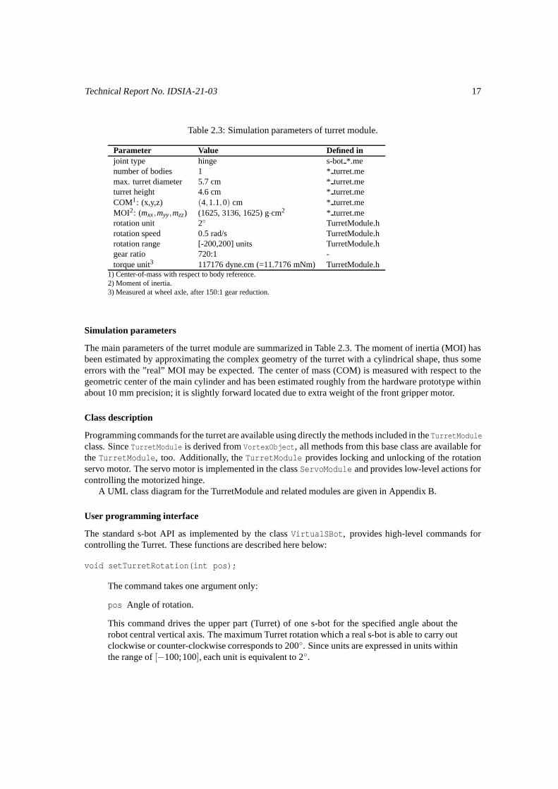
Table 2.3: Simulation parameters of turret module.
Parameter Value Defined injoint type hinge s-bot *.menumber of bodies 1 * turret.memax. turret diameter 5.7 cm * turret.meturret height 4.6 cm * turret.meCOM1: (x,y,z) (4,1.1,0) cm * turret.meMOI2: (mxx,myy,mzz) (1625, 3136, 1625) g·cm2 * turret.merotation unit 2◦ TurretModule.hrotation speed 0.5 rad/s TurretModule.hrotation range [-200,200] units TurretModule.hgear ratio 720:1 -torque unit3 117176 dyne.cm (=11.7176 mNm) TurretModule.h
1) Center-of-mass with respect to body reference.2) Moment of inertia.3) Measured at wheel axle, after 150:1 gear reduction.
Simulation parameters
The main parameters of the turret module are summarized in Table 2.3. The moment of inertia (MOI) hasbeen estimated by approximating the complex geometry of the turret with a cylindrical shape, thus someerrors with the ”real” MOI may be expected. The center of mass (COM) is measured with respect to thegeometric center of the main cylinder and has been estimated roughly from the hardware prototype withinabout 10 mm precision; it is slightly forward located due to extra weight of the front gripper motor.
Class description
Programming commands for the turret are available using directly the methods included in the TurretModuleclass. Since TurretModule is derived from VortexObject, all methods from this base class are available forthe TurretModule, too. Additionally, the TurretModule provides locking and unlocking of the rotationservo motor. The servo motor is implemented in the class ServoModule and provides low-level actions forcontrolling the motorized hinge.
A UML class diagram for the TurretModule and related modules are given in Appendix B.
User programming interface
The standard s-bot API as implemented by the class VirtualSBot, provides high-level commands forcontrolling the Turret. These functions are described here below:
void setTurretRotation(int pos);
The command takes one argument only:
pos Angle of rotation.
This command drives the upper part (Turret) of one s-bot for the specified angle about therobot central vertical axis. The maximum Turret rotation which a real s-bot is able to carry outclockwise or counter-clockwise corresponds to 200◦. Since units are expressed in units withinthe range of [−100;100], each unit is equivalent to 2◦.

Technical Report No. IDSIA-21-03 18
The invocation of this command instructs a low-level controller thread (called by the classServoModule) to rotate the simulated turret to a desired position indicated by pos. Noticethat, as it happens with the real s-bot, it may take some time to reach the desired positionbecause of the finite rotation speed.
int getTurretRotation(void);
This command reads the angle about which the s-bot turret has rotated with respect to thedefault zero rotation. This particular position corresponds to the robot turret aligned with theunderlying treels and with its front gripper right on top of ground sensor 0.
It does not take any argument but it returns the turret rotation angle in units within the rangeof [−100;100].
int getTurretRotationTorque(void);
This command reads the rotation torque of the robot turret. It does not take any argumentand it returns an integer within the range of [−127;127] expressing the torque read. Refer toTable 2.3 for the units.
2.2.3 Front Gripper Module
Description
The front gripper enables one s-bot to grasp an object or another fellow s-bot, in which case s-bots build aphysical connection. Connections can be rigid enough to allow one robot to lift the gripped s-bot.
Modeling
The simulated Front Gripper has been implemented in three increasing levels of detail:
1. Fast/Simple: The Fast and Simple s-bot models do not explicitly incorporate a Front Gripper modelbut connection between two s-bots can still be achieved by creating a static joint in the XML filedescription. Note that this approximation is static, i.e. new connections cannot be made duringsimulation. This is the preferred connection model for the Fast and Simple reference models.
2. Medium: The Front Gripper is approximated in this case by a ”sticking element”, a rectangular boxwhich is able to attach to other s-bots in a ”magnet-like” fashion. The box is hinged on the turretand can be elevated up and lowered down. This extra degree of freedom is important for coordinatedmotion tasks on rough terrain. Since this implementation model is defined as a separate geometricmodel connected to the Turret with a hinge, it introduces one extra dynamical body. Note that thisapproximation is dynamic, i.e. connections can be turned on/off during simulation. It is intended tobe used for the Medium reference model.
3. Detailed This Front Gripper model approximates the hardware gripper in very fine detail. It ischaracterized by
• a hinge for elevating or lowering the gripper arm,
• two jaw elements (upper and lower) with which to realize the gripping (opening and closing),
• integrated optical light barrier.
This gripper implementation introduces 3 extra dynamical bodies: one for the arm body and two forthe jaws. This approximation is dynamic by nature, i.e. connections can be created and cancelled byopening and closing the jaws. It is intended to be used for the Detailed reference model.

Technical Report No. IDSIA-21-03 19
Figure 2.5: Simulated models of Front Gripper. Left to right: Medium Front Gripper side and ISO view;Detailed Front Gripper side and ISO view.
Table 2.4: Simulation parameters of front gripper module.
parameter value defined injoint type hinge * turret.menumber of bodies 1 (medium) Front Arm/Coarse,, 3 (detailed) Front Arm/Detailedgrasping force at jaw 15 N Front Arm/Detailed/front-arm.mearm elevation torque 0.5 Nm * turret.mezero set point 15◦ -jaw element speed 1 rad/s GripperModule.cpprotation speed 0.87 rad/s GripperModule.cpplight barrier max sensitivity 40 mm GripperModule.cpplight barrier min sensitivity 1 mm GripperModule.cpp
Figure 2.5 shows the three simulation models for the s-bot Front Gripper.Using any of the gripper simulation models, a user can create connections between s-bots. during
simulation. The sizes of the different gripper approximations have been adjusted, so that the distancebetween two connected s-bots using any of the gripper models are the same.
Comparison with hardware
The detailed version of the Front Gripper has been calibrated with the elevation speed of the arm and theopening/closing speed of the jaws. In this respect, the simulation model shows a similar “time-delay” bet-ween issuing, for example, the gripper command “close” and the actual time that the gripper has “closed”.This “time-delay” is not present in the Simple and Medium representations as the sticking element sets itsstate immediately.
Simulation parameters
The simulation parameters for the gripper models are summarized in Table 2.4.
State variables
Abstracting from the particular model selected, the simulation state of the s-bot gripper can be characterizedby the following (implicit) state variables:
〈elevation,aperture,grippedBody〉 (2.2)
where

Technical Report No. IDSIA-21-03 20
elevation the elevation angle of the gripper armaperture the opening angle of jaw elementsgrippedBody the body ID of the connected object
Class description
The Simple, Medium and Detailed Front Gripper models are implemented as derived classes (GripperModuleSticky, GripperModuleWithArm and GripperModuleWithJaws) of the common base class GripperModule andprovide extra methods that are not available through the standard s-bot API (Appendix A). Developers whoneed to extend or modify the default simulated gripper functionalities need to access these classes directly.
Notice that the ID of the connected object in the state variable grippedBody (Eq. 2.2) is not availablein the real robot: it is only present in simulation. For this reason, the standard API does not allow accessto grippedBody and its value can only be accessed through the class GripperModule. The MdtBodyID ofthe gripped body (state variable grippedBody in Eq. 2.2) may be retrieved using the command
GripperModule*::getGrippedBody().
The connection between one robot’s front gripper and the other robot’s light ring attachment is in thehardware s-bot purely mechanical. Ideally the Detailed Gripper model using the jaws should replicate thisbehaviour but, because of the large forces involved in simulation, such a tight grip can not be reproduced.An alternative implementation realizing a rigid grip uses dynamic joints. This technique allows to createa rigid joint between the gripper and the other s-bot every time a rigid connection between two s-bots isrequested. The dynamic connection of the sticky elements (in the simple and medium gripper models)works exactly in this way.
Sticky elements (with MATERIAL ID=5) can only stick to “stick-able” objects (with MATERIAL ID=4)and these are determined by setting the appropriate material ID in the model section of the XML file. A con-nection, i.e., the creation of a dynamic joint, can only occur when a “sticking-element” is in contact with a“stick-able” object and at the same time a closing command is issued to the gripper (setGripperAperture(0)).If the element is not in contact with a “stick-able” object, a dynamic joint is not created. The sticky elementis implemented in the class StickyElement.
A UML class diagram for the GripperModule and related modules are given in Appendix B.
User programming interface
End-users should control the gripper using gripper commands as defined by the standard s-bot interfacethrough the class VirtualSBot. All gripper implementations accept these commands but return a voidaction if a command is irrelevant. The Simple and Medium Gripper models overload the jaw commandswith equivalent commands to control their sticky elements.
void setGripperElevation(int elevation);
This command sets the elevation of the robot Front Gripper Arm expressed in sexagesimaldegrees.
It takes one argument:
elevation Angle of elevation in degrees.
Because of physical constraints, the real gripper arm elevation is limited within the range of[−90;90]. Within Swarmbot3d, any value outside such a range is automatically cut to thenearest end. This means, for instance, that requesting an elevation of 100◦ would result instopping the arm actuation as soon as 90◦ is reached.

Technical Report No. IDSIA-21-03 21
The actual action is performed by a low-level background thread (in the class ServoModule)that implements the control of the elevation actuator. Notice that it takes a finite time to reachthe desired elevation position. If the gripper arm is obstructed in some way, and the elevationposition cannot be reached, the thread is killed after a timeout period. For the Minimal Gripper,elevation actions result in a void action and any return value is undefined.
int getGripperElevation(void);
This command reads the current gripper arm elevation with respect to the zero elevation whichoccurs when the arm and the Turret are aligned. It does not take any argument but it returns aninteger within the range of [−90;90].
void setGripperAperture(int aperture);
This command sets the aperture of the Front Gripper Arm jaws. The value specified corre-sponds to the sexagesimal angle between one jaw and the Front Arm central axis.
It takes one argument:
aperture Angle of aperture in degrees.
The maximum angle a real jaw can reach is 45◦. This means that the maximum bite widthreachable is 90◦. Hence, aperture can be any integer within the range of [0;45].
As shortly mentioned above, the aperture command also controls the ”sticking-elements” ofthe Medium Gripper model. Although this last does not have jaw elements, setting the apertureto any non-zero value results in ”unsticking” any previous connection, and setting aperture=0results in creating a dynamic joint if the element is in contact with some stick-able object.
int getGripperAperture(void);
This command reads the current elevation of one Front Gripper Arm jaw, which doubled be-comes the overall aperture of the gripper. It does not take any argument and it returns aninteger within the range of [0;45].
int getGripperElevationTorque(void);
This command reads the gripper torque. It does not take any argument and it returns a valuewithin the range of [−127;127]. It may be used, for example, to estimate the weight of grippedobjects.
void getGripperOpticalBarrier(unsigned *internal,unsigned *external,unsigned *combined);
This command reads the optical barrier of the front gripper arm. The readings are withinthe range of [0;700] with 0 representing total obstruction and 700 representing open emptygripper.
It does not take any input parameter, but it returns three values:
internal This is a pointer to the reading representing the internal barrier sensor.
external This is a pointer to the reading representing the external barrier sensor.
combined This is a pointer to the reading representing the internal and external combinedbarrier sensor reading.

Technical Report No. IDSIA-21-03 22
Figure 2.6: The Side Arm is modeled as a 3D extendible/retractable scissor-like mechanism. From left toright: side, top and isometric view.
2.2.4 Flexible Side Arm Module
Description
The hardware design specifications (Workpackage 2, Milestone 3) describe the Flexible Side Arm as a 3Dextendible/retractable scissor-like mechanism actuating three inner joints. An extra gripping device is alsolocated at the utmost tip of this structure. The connection to other s-bot occurs by closing this extra gripper,whereas, conversely, a disconnection occurs by opening it.
Compared to the Front Gripper Arm, the Side Arm is intended for a different purpose. While theformer is rigid and powerful enough to lift another s-bot, the latter is flexible and it allows links extendedover bigger distances. The Flexible Arm is not rigid nor strong enough to lift or push objects and it ismainly intended to be used, when fully extended, either to pull objects or to provide fellow s-bots withlateral support for creating stable connected swarm structures. Also the gripping force is reduced to 1 N (itis 15 N for the rigid Front Gripper Arm).
Modeling
The only simulation model of the Side Arm is a fully detailed one which replicates all elements of thescissor-like structure including a detailed jawed gripper element (Figure 2.6). This is mechanically speak-ing the most complex part of the simulated s-bot: featuring 11 dynamical bodies and using 12 joints. Theimplementation of the Flexible Arm with this level of detail introduces a fair amount of computationaloverhead in the simulator and can greatly affect the efficiency of the overall simulator. The use of theFlexible Arm simulation module should therefore only be included for experiments using the Flexible SideArm explicitly.
As far as control is concerned, the Side Arm module simulates 5 servo motors: three independentservo-motors for controlling the extension of the arm, and two controlling the jaws.
Simulation parameters
The simulation parameters for the Side Arm are summarized in Table 2.5. The elevation torque of theside-arm (0.04 Nm) is much less compared to that of the rigid front gripper (0.5 Nm). Also the grippingforce is reduced to 1 N from the 15 N of the rigid gripper.
State variables
The state of a side arm might be synthesized with the following tuple
〈φs,γs,ds,ψs〉, (2.3)

Technical Report No. IDSIA-21-03 23
Table 2.5: Simulation parameters of flexible Side Arm module.
parameter value defined innumber of motors 5 side arm.menumber of joints 12 side arm.menumber of bodies 11 Side Arm/horizontal torques 0.07 Nm side arm.mevertical torque 0.04 Nm side arm.meunit 0.458◦ SideArmModule.cppgrasping force at jaw 1 N side-arm-gripper.me
where φs,γs are the elevation and rotation of the Side Arm structure relative to its rest position, ds is thecurrent depth of the Side Arm, and ψs is the current aperture angle of the jaws.
Class description
The Side Arm is implemented in the class SideArmModule that contains 5 simulated servo-motors, threefor controlling the arm position and two synchronized simulated servos that control the gripper jaws. Theservos are accessible as members of the class ServoModule which provides low-level threaded actionsfor controlling the motorized hinges to rotate to a specific angular position (similar to the hardware PICcontrollers).
A UML class diagram for the SideArmModule and related modules are given in Appendix B.
User programming interface
The state of the simulated Side Arm can be controlled and read out using the standard API commands(Appendix A):
void setSideArmPos(int elevation, int rotation, int depth);
This command positions the Flexible Side Arm in space by setting the elevation and rota-tion angle of the main Side Arm axis, and by setting the outward/inward depth it has to pro-trude/retract, respectively.
It takes three input parameters:
elevation This represents the tilting angle in sexagesimal degrees with respect to the hori-zontal Flexible Arm resting position.
rotation This represents the rotating angle in sexagesimal degrees with respect to the Flex-ible Arm resting position which is 110◦ from the Front Gripper Arm main axis.
depth This is the depth to which the gripper at the end tip of the arm has to be protruded orretracted.
Notice that the command does not directly modify the state variables as described in Eq. 2.3but use the three servo motors to position the Side Arm. Inverse kinematic control is needed tomap servo-motor positions elevation, rotation and depth to the corresponding state variables.
void getSideArmPos(int *elevation, int *rotation, int *depth);
This command reads the current position of the Flexible Side Arm.
It does not take any input parameters but it returns three values:

Technical Report No. IDSIA-21-03 24
elevation Tilting angle of the arm main axis with respect to the horizontal rest position.
rotation Rotating angle of the main axis with respect to the resting position (110◦ spacefrom the Front Gripper Arm main axis).
depth Protruding or retracting depth to which the gripper of the Flexible Arm has to be lo-cated.
void getSideArmTorque(int *elevation, int *rotation, int *depth);
This command reads the current torque to which the Flexible Arm motors are subjected.
It takes no input parameters and it returns three values:
elevation This is a pointer to the torque reading of the elevating actuator.
rotation This is a pointer to the average torque reading of the actuators performing horizon-tal rotations.
depth This is a pointer to the difference between the torque of the actuators performing hori-zontal actuation.
void setSideArmOpened(void);
This command actuates the Side Arm Gripper so as to open up completely its jaws. It does nottake any input parameters nor it returns any value.
As opposed to the Front Gripper, the user API does not allow to control the aperture of theSide Gripper by specifying an angle: in case it is necessary, the user should refer to the theimplementation class.
void setSideArmClosed(void);
This command actuates the Side Arm Gripper so as to close completely its jaws. It does nottake any parameters, nor returns anything.
void getSideArmOpticalBarrier(unsigned *internal,unsigned *external,unsigned *combined);
This command reads the optical barrier of the Flexible Gripper Arm. The readings are withinthe range of [0;700] with 0 representing total obstruction and 700 representing open emptygripper.
It does not take any input parameters and it returns three values:
internal This is a pointer to the reading representing the internal optical barrier sensor read-ing.
external This is a pointer to the reading representing external optical barrier sensor reading.
combined This is a pointer to the reading representing the internal and external combinedoptical barrier sensor reading.
2.2.5 Camera Module
Description
The real s-bot has an omni-directional camera mounted at the top of the Turret which provides a fish-eyeview of the surrounding environment. The camera looks at a spherical mirror suspended above it at the topof a vertical transparent tube. The camera is mainly intended to monitor the surrounding environment andto detect the colors of the light-ring of other s-bots.

Technical Report No. IDSIA-21-03 25
Figure 2.7: From left to right: (a) The simulated Camera is place on top of the center pole. (b). ISO-viewof scene. (c). Simulated fish-eye camera view seen from center s-bot.
Modeling
Two simulation models are available for the camera.
1. Fast/Simple: A high-level Camera implementation (FakeCamera) which simulates methods forhigh-level recognition of observable objects. The fake camera senses all LED’s that can be seenin a certain scope maximum distance and vertical sensing angle. It is placed on top of the s-bot andfixed to the body with a vertical offset. It is a 360◦ camera. The LEDs are placed around the s-botsbody radius and they can have different color.
This implementation skips resource-intensive low-level image processing computation and may bemuch more efficient if only high-level cognition function of object is required. It is intended to beused for the Fast and Simple reference models.
2. Medium/Detailed: A low-level Camera implementation (RawCamera) which returns an array ofvalues representing color values of a CCD camera (as in the real s-bot). This camera has beenimplemented in the simulator by placing the OpenGL camera at the position of the spherical mirrorat the top of the tube. Because the OpenGL libraries do not provide a command to generate an omni-directional view directly, 4 snapshots are taken, each covering a 90◦ field of view. The 4 snapshotsare stitched and mapped to polar coordinates to simulate a fish-eye view. It is intended to be used forthe Medium and Detailed reference models.
The cameras are instantiated by the constructor of the robot/VirtualSBot class. Figure 2.7 showsthe camera fixture (the center pole structure), an arbitrary scene, and the omni-directional camera view asseen from the central s-bot.
Comparison with hardware
The stitching procedure of the RawCamera is not perfect and leaves some artifacts at the stitched boundaries.These artifacts are known to be more pronounced at inclined postures of the s-bot.
Simulation parameters
The simulation parameters for the two simulated types of Camera are summarized in Table 2.6 and 2.7.
State variables
The simulation state describes the current camera view and comprises the list of viewable objects for theFakeCamera, or the entire video buffer for the RawCamera.

Technical Report No. IDSIA-21-03 26
Table 2.6: Simulation parameters of raw camera module.
parameter value defined invertical offset 11.85 cm * turret.mebuffer size 640×448 (window size)
Table 2.7: Simulation parameters of the fake camera module.
parameter value defined invertical offset 5.0 cm FakeCamera.hmaximum sensor distance 1000 cm FakeCamera.hsensing vertical angle 70◦ FakeCamera.h
Class description
This raw camera module is only available by default for the medium and detailed s-bot models, and is imple-mented in the class devices/RawCamera. The fake camera is implemented in the class devices/FakeCameraand can be used on all reference s-bot models.
A UML class diagram for the CameraModule and related modules are given in Appendix B.
User programming interface
Currently, there is no camera command defined in the standard API yet and the use of the camera must bedone using the class implementations directly.
The high-level FakeCamera implementation will probably not be compatible with the standard s-botAPI and should not be used when portability to the real s-bot is in mind.
For the RawCamera, the current camera view can be read by accessing the contents of the camera bufferthrough a pointer to an array of type char (8 bits). The size of the array is 640× 448× 3, repeating thethree RGB values for each pixel of the camera pixel array.
2.2.6 Proximity Sensor Module
Description
The s-bot has 15 infra-red (IR) Proximity Sensors that can detect obstacles in the immediate neighbourhoodof one s-bot. The sensors are placed at the lower part of the Turret with angular distance of 1/18 of afull circle, but 3 sensors in front of the s-bot (where the Front Gripper is placed) are ”missing”. This isimportant, because one s-bot cannot sense its vicinity using the IR sensors along the direction of the FrontGripper.
Infrared sensors detect the amount of reflected infrared light emitted by the robot IR LED. The sensi-tivity of such sensors on the real s-bot has a sensitivity volume which can be approximated by a cone withan angle of about 40◦ and a range of about 200 mm.
Modeling
The simulator provides two implementations of the infrared proximity sensors.

Technical Report No. IDSIA-21-03 27
Figure 2.8: From left to right: (a) A single IR sensor is modeled using 5 probing rays. (b) ISO-view ofs-bot using Proximity Sensors. (c) GUI frame showing Proximity Sensor values.
1. Fast/Simple: A sample-based implementation using a look-up-table (LUT) is available. This classimplements sampling techniques applied to generic sensors which depends only on the relative posi-tions of s-bots (no walls, obstacles, or shadowing is taken into account in this first implementation).The LUT values need to be measured separately performing robotic experiments. Because currentlyonly 2D LUT values are available, this type of proximity sensor is mainly meant for simulationsemploying the Fast and Simple reference models on flat plane.
2. Medium/Detailed: The ray-tracing based Proximity Sensor simulation module models each infraredsensor using 5 rays that are distributed in the cone sensitivity volume: 1 central ray, and 4 peripheralrays on a cone surface (Figure 2.8). Proximity is detected by monitoring the intersection of each linewith other bodies (e.g. other s-bot or walls). This type of proximity sensor can be used independentlyfrom terrain type, and has been integrated in the Medium and Detailed reference models.
Because of its general validity in complex situations, the ray-tracing based sensing model is preferredabove the sample-based implementation in all but simple environments. For these last, the sample basedapproach may be more efficient. The rest of this section discusses only the ray-tracing based proximitysensor model.
Comparison with hardware
In the ray-tracing based implementation, for each sensor, 5 rays detect any intersection of nearby objectsand compute an average distance value which is then converted to an integer sensor response. Such aresponse has been calibrated using linear regression (in a log-log space) using measured distance responsesof 3 different IR sensors using a total of 33 measured values.
Based on the experimental data, a linear fit in log-log space appeared sufficient to provide an adequatefit using the regression function:
y = exp(a+b∗ log(x)) (2.4)
where y is the Proximity Sensor response, x is the distance value, and a and b are the regression parameters.The best fit was found using a nonlinear least squares Marquardt-Levenberg algorithm. The final set ofregression parameters and their asymptotic standard errors found were:
a = 8.44352 ± 0.2134 (2.528%)
b = −0.777545 ± 0.05392 (6.935%). (2.5)
One difference between the simulated IR sensors and the real ones is that while the latter detect anyobject within a sensitivity cone, the former suffer from the so-called ”dead spot”, i.e., the space in which

Technical Report No. IDSIA-21-03 28
Table 2.8: Simulation parameters of the Proximity Sensor module.
Parameter Value Defined innumber of sensors 15 modules/ProximitySensorModuleminimum sensing distance 0.2 cm modules/ProximitySensorModulemaximum sensing distance 20 cm modules/ProximitySensorModuleray-tracing cone angle 30◦ devices/IRSensorray-tracing per sensor 5 devices/IRSensornoise level uniform 10 % devices/IRSensor
small objects remain undetected because they lie just in between rays. Although the sensitivity field ofthe IR sensor was measured to be about 40◦, it was decided to place the peripheral ray-tracing rays at 30◦
angles around the center ray. The dead spot is in this way reduced. Indeed, it could be reduced even furtherby using more probing rays at an increase of computational costs.
Another difference which has been observed is that real sensors are sensitive to the color of the reflect-ing surface, whereas the simulated ones (solely based on intersection distance) are not.
Uniform noise of 10% has been added to the distance measurements in order to simulate sensor noise.Additionally, the hardware IR sensors seem to suffer from noise due to cross-talk with the power supply butthis is expected to get improved in future designs. Thus, such a contribution to the noise in the simulatorhas not been modeled.
Simulation parameters
The simulation parameters for the simulated IR Proximity Sensors are summarized in Table 2.8.
State variables
The simulation state of the Proximity Sensor describes the current proximity sensor values and can berepresented by
〈 sensor[15] 〉, (2.6)
where sensor[i] is the sensor reading of the i-th proximity IR sensor.
Class description
The IR proximity module is implemented by the class ProximitySensorModule. The sensor objects areimplemented by the class devices/IRSensor. The position of the sensor is determined by the IR SENSOR xxtags in the * turret.me XML file. The x-axis of its model geometry determines the normal (sensing) di-rection of the sensor.
A UML class diagram for the ProximitySensorModule is given in Appendix B.
User programming interface
The standard s-bot interface provides commands to read the value of the Proximity Sensors. To read asingle IR sensor use the command
unsigned getProximitySensor(unsigned sensor);

Technical Report No. IDSIA-21-03 29
Figure 2.9: Left: Capsized robot showing 4 Ground Sensors at the bottom of the Treels. Right: S-Bot usingFront Ground Sensor to detect a step.
This command reads the current value of the specified IR Proximity Sensor. It takes one inputparameter and it returns one unsigned integer encoding the distance to the hit target within therange of [0;8191]:
sensor IR labelling number within the range of [0;14].
The distance encoded is not linearly proportional to the actual distance. One object 150 mmaway produces a reading of 20, another one at 50 mm away induces a reading of 50, yet anotherone at 10 mm produces a reading of 1000, and finally one at 5 mm away produces a readingof 3700.
void getAllProximitySensors(unsigned sensors[15]);
This command reads the value of all IR Proximity Sensors and dumps them into an array. Allreadings are within the range of [0;8191]. It does not take input parameters but it returns itsreadings in an array of 15 locations:
sensors Array of distances to objects.
void setProximitySamplingRate(SamplingRate rate);
This command sets the IR Proximity Sensor sampling rate but for the simulator this commandis irrelevant because in the simulator the IR values are calculated in real time. It takes oneinput parameter:
rate Sampling rate expressed in terms of SAMPLING RATE xx values.
2.2.7 Ground IR Sensor Module
Description
Four IR sensors are placed at the bottom of the Treels body looking downward to the ground. These GroundSensors can be used to detect terrain conditions such as holes or edges. The left image in Figure 2.9 showscap-sized s-bot showing its 4 ground sensors at the bottom. The right image in Figure 2.9 shows the use ofthe front ground sensor to detect a step during navigation.
Technical Report No. IDSIA-21-03 30
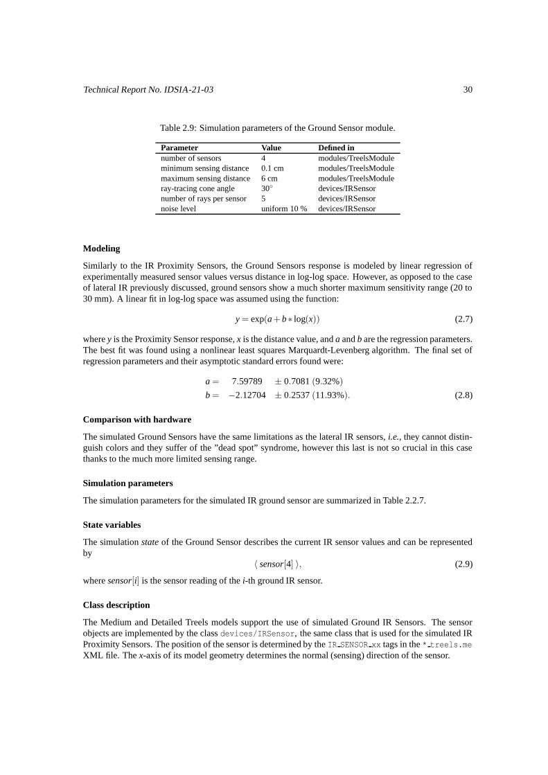
Table 2.9: Simulation parameters of the Ground Sensor module.
Parameter Value Defined innumber of sensors 4 modules/TreelsModuleminimum sensing distance 0.1 cm modules/TreelsModulemaximum sensing distance 6 cm modules/TreelsModuleray-tracing cone angle 30◦ devices/IRSensornumber of rays per sensor 5 devices/IRSensornoise level uniform 10 % devices/IRSensor
Modeling
Similarly to the IR Proximity Sensors, the Ground Sensors response is modeled by linear regression ofexperimentally measured sensor values versus distance in log-log space. However, as opposed to the caseof lateral IR previously discussed, ground sensors show a much shorter maximum sensitivity range (20 to30 mm). A linear fit in log-log space was assumed using the function:
y = exp(a+b∗ log(x)) (2.7)
where y is the Proximity Sensor response, x is the distance value, and a and b are the regression parameters.The best fit was found using a nonlinear least squares Marquardt-Levenberg algorithm. The final set ofregression parameters and their asymptotic standard errors found were:
a = 7.59789 ± 0.7081 (9.32%)
b = −2.12704 ± 0.2537 (11.93%). (2.8)
Comparison with hardware
The simulated Ground Sensors have the same limitations as the lateral IR sensors, i.e., they cannot distin-guish colors and they suffer of the ”dead spot” syndrome, however this last is not so crucial in this casethanks to the much more limited sensing range.
Simulation parameters
The simulation parameters for the simulated IR ground sensor are summarized in Table 2.2.7.
State variables
The simulation state of the Ground Sensor describes the current IR sensor values and can be representedby
〈 sensor[4] 〉, (2.9)
where sensor[i] is the sensor reading of the i-th ground IR sensor.
Class description
The Medium and Detailed Treels models support the use of simulated Ground IR Sensors. The sensorobjects are implemented by the class devices/IRSensor, the same class that is used for the simulated IRProximity Sensors. The position of the sensor is determined by the IR SENSOR xx tags in the * treels.meXML file. The x-axis of its model geometry determines the normal (sensing) direction of the sensor.

Technical Report No. IDSIA-21-03 31
User programming interface
The standard s-bot API (Appendix A) defines three commands with regard to ground sensors:
unsigned getGroundSensor(unsigned sensor);
This command reads the value of one of the specified Ground Sensor. It takes one inputparameter and it returns one unsigned integer within the range of [0;255]:
sensor Ground IR Sensor number within the range of [0;3].
The distance to the ground encoded in the reading of one ground IR sensor is not linearlyproportional to the actual distance. A ground 6 mm away provides a reading of 1, one at 2 mmproduces a reading of 25, and one at 1 mm distance generates a reading of 100.
void getAllGroundSensors(unsigned sensors[4]);
This command reads the value of all Ground Sensors and dumps them into an array of 4elements. It takes no input parameters and it returns the Ground Sensor readings into thespecified array:
sensors Array of distances to objects.
void setGroundSamplingRate(SamplingRate rate);
This command sets the sampling rate of the IR Ground Sensors. However for the simulatorthis command is irrelevant because the IR values are calculated within the simulator in realtime. It takes one input parameter and it does not return anything:
rate Sampling rate expressed in terms of SAMPLING RATE xx values.
2.2.8 Light Ring Module
Description
Around one s-bot’s Turret, there is a semi-translucent ”light ring” which serves multiple purposes.
1. It can act as a gripper attachment for the Front and Side Arm grippers of other robots so as to createfixed or flexible swarm-bot structures,
2. It features 8 colored light groups that can display patterns of color. Each group can be controlledindependently to blink and its color can be specified independently using RGB values. The light ringis primarily intended for communication between other s-bots that can recognize the colors using theomni-directional camera.
3. Each sector also includes a Light Sensor that can measure the intensity of (green) ambient light.Using these Light Sensors, one s-bot can measure the direction and intensity of the light in its envi-ronment, for example for navigation tasks.

Technical Report No. IDSIA-21-03 32
Figure 2.10: Left to right: Detailed s-bot model showing red, green and blue lights, respectively
Table 2.10: Simulation parameters of Light Ring module.
Parameter Value Defined innumber of LED 8×3 modules/LEDModuleLED unit 0.8 mCd modules/LEDModulemaximum LED intensity 12 mCd (= 15 units) modules/LEDModulenumber of sensors 8 modules/LEDModulesensor unit 0.1685 mCd/cm2 modules/LEDModulemaximum sensor unit 700 units modules/LEDModulemaximum blink frequency 5 Hz controllers/LEDController
Modeling
The simulated Light Ring is available in the Medium and Detailed s-bot reference models. It is modeledas part of a <COMPOSITE GEOMETRY> in the Turret XML description: this avoids creating an additionaldynamic body to define it.
The light intensity of the elements composing a ring are visualized by modifying the graphics color ofthe objects. Light calculations are based on intensity variables defined in the class devices/Light. Theclass provides methods for calculating the illuminance due to the light source at a some relative positionby weighing the source intensity by its inverse squared distance from illuminance position to the source.Light intensities are calculated using milli-candela (mCd) as the unit of computation.
Comparison with hardware
Although the hardware light ring module has a maximum blinking frequency of 10 Hz (see standard s-botAPI, Appendix A), the simulated Light Ring can only handle a maximum blinking frequency of 5 Hz.
Simulation parameters
The simulation parameters of the Light Ring module are summarized in Table 2.10. The sensor and LEDparameters are based from specifications of the hardware.
State variables
Taking into account the description of the Light Ring module, the simulation state of the Light Ring canbe identified with the following tuple
〈 r[8],g[8],b[8],blink[8] 〉 (2.10)

Technical Report No. IDSIA-21-03 33
where
r[i] is the red value of LED group i,g[i] is the green value of LED group i,b[i] is the blue value of LED group i,blink[i] is the blink frequency of LED group i
Class description
The Light Ring module is implemented by the class LightRingModule (defined in modules/LEDModule).Light blinking is controlled by a single thread for all 8 groups and it is implemented by the class controllers/LightRingBlinkAction.
A UML class diagram for the LightRingModule is given in Appendix B.
User programming interface
A user can control and read the simulation state of the Light Ring using the following functions as definedin the standard s-bot API (Appendix A):
unsigned getLightSensor(unsigned sensor);
This command reads the value of the specified light sensor within the range of [0;700] with 0representing full darkness and 700 representing full light. It takes one input parameter and itreturns one unsigned integer:
sensor Light sensor number within the range of [0;7].
void getAllLightSensors(unsigned sensors[8]);
This command reads the value of all light sensors and dumps them into one array of 8 elements.It takes no input parameters and it returns one array of unsigned integers:
sensor Array of light intensities.
void setLightColor(unsigned light, unsigned r, unsigned g,unsigned b, BlinkingRate blink);
This command sets the color of a light emitter with a specified blinking rate. It takes 5 inputparameters and it does not return anything:
light Light sensor number within the range of [0;7].
r Red light intensity within the range of [0;15].
g Green light intensity within the range of [0;15].
b Blue light intensity within the range of [0;15].
blink Blinking rate expressed in terms of BLINKING RATE xx values.
void setAllLightColor(unsigned r[8], unsigned g[8], unsigned b[8],BlinkingRate blink[8]);
This command sets the color of all light emitters. It takes 4 input parameters and it returnsnothing:

Technical Report No. IDSIA-21-03 34
r Array of red light intensities with each value expressed within the range of [0;15].
g Array of green light intensities with each value expressed within the range of [0;15].
b Array of blue light intensities with each value expressed within the range of [0;15].
blink Array of blinking rates with each value expressed in terms of BLINKING RATE xx val-ues (see interface/sbot.h).
void setSameLightColor(unsigned r, unsigned g, unsigned b,BlinkingRate blink);
This command sets the same color for all light emitters. It takes 4 input parameters and itreturns nothing:
r Red light intensity expressed within the range of [0;15].
g Green light intensity expressed within the range of [0;15].
b Blue light intensity expressed within the range of [0;15].
blink Blinking rate expressed in terms of BLINKING RATE xx values (see interface/sbot.h).
void setLightSamplingRate(SamplingRate rate);
This command sets the sampling rate of the light sensors. It takes one input parameter and itreturns nothing:
rate Sampling rate expressed in terms of SAMPLING RATE xx values (see interface/sbot.h).
In the simulator this command is irrelevant as (for efficiency reasons) the light sensors areupdated only when a reading command is issued.
2.2.9 Inclinometer Module
Description
The Inclinometer allows reading of the s-bot pose. Such a device provides information needed for stablenavigation on rough terrain.
Modeling
The inclination is defined as the pitch (i.e., forward inclination) and roll (i.e., lateral inclination) of thetracks system.
Comparison with hardware
No comparison has yet been performed.
Simulation parameters
No model parameters.

Technical Report No. IDSIA-21-03 35
State variables
The inclination state of the s-bot can be identified as the following tuple:
〈roll, pitch〉 (2.11)
where
roll is the lateral inclination andpitch is the forward inclination.
Class description
The Inclinometer is implemented by the class devices/inclinometer and it simply returns the pitch/rollvalues based on the MdtBody orientation. The orientation of the MdtBody is read using Vortex librariesdirectly.
User programming interface
Currently, the standard s-bot API (Appendix A) defines two commands regarding the inclination state ofthe s-bot:
void getSlope(int *pitch, int *roll);
This command reads the slope pitch and roll angles of a robot. It takes no input parametersand it returns two values:
pitch Pointer to the pitch angle expressed within the range of [−180;180].
roll Pointer to the roll angle expressed within the range of [−180;180].
void setSlopeSamplingRate(SamplingRate rate);
This command sets the sampling rate of the slope sensor. It takes one input parameters and itdoes not return anything:
rate Sampling rate expressed in terms of SAMPLING RATE xx values.
In the simulator this command does not perform anything because the inclination values arenot buffered, but read in real-time from the simulation state.
2.2.10 Sound Module
Description
A real s-bot hosts on top of its Turret and at the base of the camera fixture three microphones placed aboutthe central pole at 120◦ apart from each other. A speaker is available to produce sound. The sound moduleis intended for simple communication and localization.

Technical Report No. IDSIA-21-03 36
Figure 2.11: At the bottom of the camera pole, three microphones are placed 120◦ from each other aboutthe central pole.
Modeling
A rigorous sound implementation based on wave PCM is not suitable because the nominal simulation timestep 10 ms would only be able to simulate sinusoidal waves with a maximum frequency of 50Hz.
A simplified frequency-based sound module has been implemented in alternative within Swarmbot3d.Each virtual microphone computes its sound intensity by summing up all sound source contributions withina frequency band weighted by the inverse squared distance between microphone and sound source. Theimplementation is the same as the one discussed in another project publication [1], using the (single source)sound amplitude function
A = ∑s
1−0.9αS/π1+D2
S/p0(2.12)
where αS is the angle between the microphone direction and the direction of the sound source S, and DS isthe geometric distance between microphone and source. The total perceived amplitude (TPA), accordingto this model is computed using
T PA = ∑s
21+ exp(−∑i Ai)
−1 (2.13)
where ∑i sums over all sound contributions Ai from the other robots i (excluding itself).Lower and upper frequency limits can be set to determine the band width. Currently, speaker is limited
to emit sound of a certain intensity at one single frequency at a time.
Comparison with hardware
At the time of writing the present document, the hardware sound module is still in the early testing phase(Milestone 5, ”Hardware Analysis”). Implementation and API changes of the simulated Sound module areexpected as soon as the hardware design is completed.
Simulation parameters
The simulation parameters of the Sound module are summarized in Table 2.11.

Technical Report No. IDSIA-21-03 37
Table 2.11: Simulation parameters of sound module.
Parameter Value Defined innumber of microphones 3 modules/SoundModule*number of speakers 1 modules/SoundModule*uniform noise 10% modules/SoundModule*
State variables
Taking into account the description of the simple frequency-based Sound module, the simulation state ofthe Sound module can be identified with the following tuple
〈center, intensity, f requency〉 (2.14)
where
center is the center position of the sound source,intensity is the current sound intensity,f requency is the frequency of the sound.
Class description
The Sound module is specified by a base class modules/SoundModule and it is implemented by the de-rived classes SoundModuleSimple and SoundModuleComplex. The first implementation includes a binary,omni-directional speaker and a number of uni-directional microphones placed in a circle with a radial offsetabout the s-bot. Currently, only s-bots are checked as sources of sound.
The second implementation in SoundModuleComplex allows specification of the placement of micro-phones and sound sources based on the model descriptions specified in the XML file. Microphone andspeaker objects are implemented using the classes devices/SoundSource and devices/SoundSensor.The functionality is the same as the one offered by the simple implementation.
User programming interface
Currently, the standard s-bot API defines two commands for streaming audio files to the integrated speaker:
void playMusic(const char *filename);
This command plays the sound specified in filename. It takes one input parameter and it doesnot return anything:
filename String of characters representing the music file name.
void stopMusic(void);
This command has the effect of simply stopping emitting any music being played. In case nomusic file is being played, the command has no effect. It does not take input parameters and itreturns nothing.
To read the current sound intensity the following function can be used:

Technical Report No. IDSIA-21-03 38
int getIntensity(int k);
This command reads the current sound intensity at microphone k = 1,2,3. This function is notyet adopted in the standard API, but is planned in future versions. Details on this interface willbe deferred until hardware specifications are known .
2.2.11 Temperature and Humidity Sensors Module
Description
The s-bot hardware has two Temperature Sensors and two Humidity Sensors on each side of the frontgripper. The Humidity Sensor provides humidity readings with a time lag of about 4 seconds.
Modeling
Temperature and humidity simulation are outside the capabilities of the current simulator engine, andtherefore they have not been modeled in Swarmbot3d. However, these sensors are shortly mentioned inthis section for the sake of completeness.
User programming interface
The standard s-bot API provides two commands for reading the temperature and humidity sensors on theleft and right sides respectively:
void getTemperatureAndHumidityLeft( float *temperature,float *humidity);
This command in case of a real s-bot reads the left Temperature and Humidity Sensors. Such acommand is currently not implemented in the simulated s-bot, thus its use has no effect withinSwarmbot3d. It takes no input parameters and it returns two values:
temperature Pointer to the reading of the current sensed temperature expressed in degreeCelsius within the range of [−40;123].
humidity Pointer to the relative humidity reading within the range of [0;100].
void getTemperatureAndHumidityRight( float *temperature,float *humidity);
This command in case of a real s-bot reads the right Temperature and Humidity Sensors. Sucha command is currently not implemented in the simulated s-bot, thus its use has no effectwithin Swarmbot3d. It takes no input parameters and it returns two values:
temperature Pointer to the reading of the current sensed temperature expressed in degreeCelsius within the range of [−40;123].
humidity Pointer to the relative humidity reading within the range of [0;100].

Technical Report No. IDSIA-21-03 39
Table 2.12: Simulation parameters of the Battery module.
Parameter Value Defined innominal voltage 7.2 V devices/Battery.hcapacity 1400 mAh devices/Battery.h
2.2.12 Battery Voltage Meter Module
Description
The s-bot hardware is going to be powered by a lithium-ion battery that is placed between the trackswithin the Treels body. This battery provides a nominal 7.2V at 1.4 Ah, giving a total capacity of 10Wh(see Deliverable D4, ”Hardware design”). Power consumption of the robot is estimated to be below 5W,ensuring a minimal battery life of two hours.
An accurate battery voltage meter simulation may be useful to develop robot strategies that minimizepower consumption. An indication to the current power consumption may be used as a reinforcementfeed-back signal for learning algorithms.
Modeling
A simulated Battery Voltage Meter has not yet been fully implemented in the simulator but it has beenplanned for a future release. To calibrate correctly a Battery Meter, power consumption of each type ofactions need to be experimentally measured.
Comparison with hardware
In progress.
Simulation parameters
The simulation parameters of the Battery module are taken from the hardware specifications (DeliverableD4, ”Hardware design”) and they are summarized in Table 2.12.
State variables
Taking into account the description of the Battery module, the simulation state of the Battery module canbe identified with the following tuple
〈V,c〉 (2.15)
where
V is the current battery voltage,c is the battery capacity.
Class description
A rudimentary battery implementation is provided by the class devices/Battery but it has not yet beencalibrated against the real hardware specifications.

Technical Report No. IDSIA-21-03 40
User programming interface
Currently, the standard s-bot API defines a single command related to the Battery Voltage Meter:
unsigned getBatteryVoltage(void);
This command in case of a real s-bot has the effect of providing the current battery voltageexpressed in Volts. Such a command is not currently implemented within Swarmbot3d, thusits use has no effect at the moment.
It takes no input parameters and it returns one unsigned integer within the range of [0;255]encoding the current potential available from the batteries. A reading of 0 corresponds to 0Volts and a reading of 255 corresponds to 10 Volts.
2.3 Swarm Modeling
Description
Up to this point the discussion has considered just one isolated s-bot, however Swarmbot3d has beendesigned to handle simulations dealing with groups of s-bots. This section is devoted to show how tomonitor the status of an entire group of s-bots.
Notice that according to the principles of the swarm intelligence, a swarm should not be modeled asan explicit entity: swarm behaviours should emerge only as a property of the interaction among the unitscomposing a swarm.
Modeling
While a variety of statistical indicators may be used to characterize a group of robots, it is enough at thelowest level to return individual robot positions and headings together with the connectivities of the s-botswithin a swarm.
Having this in mind, it is useful to abstract the group of s-bots as a connected graph which showsthe current swarm configuration. Such a graph is constructed by enquiring all positions, headings andinterconnections holding among the s-bots. Figure 2.12 shows such an abstraction of a group of semi-connected s-bots.
Comparison with hardware
Practically, the global robot positions can be very simply monitored using an overhead camera to track therobots and compute their positions and headings. Often special markers on top of a robot are used to easeimage processing, e.g., [4].
All robot positions and headings are directly available within the simulator, thus such an approach isnot necessary. However, that could be mimicked by placing a simulated camera above a scene. This couldbe the method to test tracking algorithms developed for the real s-bot.
Simulation parameters
There are no swarm-bot parameters available because a swarm, according to the basic principles of swarmintelligence, is simply a collection of single s-bots.

Technical Report No. IDSIA-21-03 41
Figure 2.12: Left: Screenshot of multiple s-bots in semi-connected swarm configuration. Right: swarmabstraction using directed graphs.
State variables
Using the abstraction of a connected graph to represent the swarm, the swarm state can be identified withthe following tuple
〈 N, pos[N],dir[N],connection[N,N] 〉 (2.16)
where
N represents the number of s-bot units,pos[i] the position of s-bot i,dir[i] the heading of s-bot i, andconnection[i, j] the connection state between s-bot i and s-bot j.
Class description
A swarm-bot is implemented in the class robots/SwarmBot but it is a minimal class that is only intendedfor monitoring and simulation control of a swarm.
User programming interface
Based on what stated above, the current status of a swarm can be retrieved by using the following twocommands
void SwarmGetPositions (double* pos[3]);void SwarmGetHeadings (double* dir[3]);
The first command returns a list of the positions of all the s-bots whereas the second one returnsa list of all heading directions.
int SwarmGetConnectivity (int i, int j);

Technical Report No. IDSIA-21-03 42
Figure 2.13: Different simulated terrain models. From left to right: (a) s-bot on simple flat plane; (b) s-boton composite-plane terrain; (c) s-bot on true rough terrain (3D mesh).
This command returns the connection state between two s-bots. It returns 0 if s-bot i and jare not connected, 1 if they are connected using the front gripper, and 2 if they are connectedusing the flexible arm.
2.4 Environment Modeling
Besides s-bots, a simulation needs to have environments modeled, too. This last section is dedicated toshow how that is achieved within Swarmbot3d.
2.4.1 Terrain Modeling
Description
It was mentioned in an earlier section of this document that Swarmbot3d is designed to deal specially withoutdoor rough terrains. It is therefore necessary in a simulation to model simple flat planes as well as roughterrains.
Modeling
To model different environments, it can be employed either a description of a 3D mesh, or that of a simplesmooth flat plane. Notice that the latter can also be used to define a piecewise uneven terrain composed ofsmooth planes at different heights. This is useful for defining terrains with cliffs and sharp falling holes.
A 3D mesh can be realized by loading into the simulator a grey scale bitmap image of 128x128. Noticethat the grey scale worked in this case as a sort of depth map whose absolute values were constrained withina given range. Since any grey scale image of the same size can be applied, a user is given the possibility ofloading any type of terrain, whose roughness can be increased or decreased by acting on the constrainingrange mentioned above.
It should be pointed out, though, that the simulation performance is affected by the type of landscapeemployed. Indeed, it was observed that a swarm simulation using rough terrains gets much slower thanthe same simulation employing smooth planes. The reason of this behaviour is the increase of collisionchecking overhead caused by the more complex and uneven geometry of the terrain.
Figure 2.13 shows three terrain models: a simple flat plane, an uneven terrain made of a compositionof planes, and a true rough terrain based on a 3D mesh.

Technical Report No. IDSIA-21-03 43
Table 2.13: Simulation parameters of a terrain model.
Parameter Value Defined interrain type 〈plane,composite,rough〉 Resources/Ground/〈terrain〉.meheight range1 user defined Ground/rough terrain.medefault size 500×500 cm Ground/〈terrain〉.megravity (fast model) 0.0981 m/s2 World/Fast World Settings.megravity (others) 9.81 m/s2 World/World Settings.mewheel friction 12 ·104 dyne World/World Settings.me
1) Only for rough terrain type; it determines the ”roughness” of a terrain.
Comparison with hardware
The friction forces between wheels and ground have been experimentally measured by pulling one s-botusing a force meter (”Hardware Analysis”, Milestone 5).
Simulation parameters
Many environment parameters, such as gravity, material properties, and friction, need also to be correctlyset in order to have a realistic behaviour. Table 2.13 summarizes the simulation parameters of the terrainmodel. Parameter values for the simulated gravity have been set to 1/100 of the real gravity for the Fastsimulation model, and to real gravity acceleration of 9.81 m/s2 for all other models. The friction values arebased on measured experimental values.
State variables
Synthesizing the discussion outlined above, the parameters describing an environment can be organizedinto the following tuple:
〈type,roughness,gravity, friction〉 (2.17)
where
type is the type of landscape (i.e.either smooth or rough terrain),roughness describes the percentage of roughness,gravity is the gravity pull, andfriction is the coefficient of friction.
Class description
The terrain is implemented using McdRGHeightField.h as defined in the standard Vortex libraries.
User programming interface
The terrain model has no user interface. All parameterization must be specified in the XML file.Notice that if rough terrain is specified, then the current default grey scale bitmap is going to be used.
If a different one is required, then a new name has to be specified into the XML code describing the worldscene.

Technical Report No. IDSIA-21-03 44
2.4.2 Light and light sensors
Description
Because of the relative ease and simplicity, a variety of robotic experiments use lights in an environment inorder to provide directional information to a robot. Thus, it was necessary to include a light model in thesimulator.
Modeling
Rigorous light modeling, which also includes shadowing, reflection, and diffusion, is a very complex matterand it has not been implemented in Swarmbot3d. A simplified model is adopted instead. Such a modeluses the following assumptions:
• Lights are modeled as isotropic point sources (except for ambient light);
• Sensors are modeled as points;
• Light fall-off is proportional to the inverse squared distance between light and sensor;
• Light shadowing is simplified, i.e., only the direct line of sight is considered;
• No reflection of diffusion is considered;
• Light sensors can define angular sensitivity.
Note that 3D graphics rendering engines, such as OpenGL, do already implement complex lightingcalculations. However, only illumination in the visible part of the scene is calculated and therefore this isnot suitable for Swarmbot3d because the light needs to be calculated throughout the whole scene for alls-bots.
The point light illumination at a certain position is calculated by summing up contributions of all lightsources weighted by the inverse squared distance to the source. The sensor response is then calculated bymultiplying the illumination value with an angular sensitivity function. The simulator supports a maximumnumber of 512 point light objects but many light objects are already being used to model the LED of thelight ring of one s-bot.
Additionally, ambient light is modeled by adding a constant value to the illumination calculations.Care must be taken not to set the light intensities too high, because it has been observed that light
sensors (LightSensor) are over-saturated quite easily.
Comparison with hardware
Not yet calibrated with the real robot hardware.
Simulation parameters
Table 2.14 summarizes the simulation parameters of the light model.
State variables
The simulation state of a light object can be represented by the following tuple:
〈color,max intensity, intensity〉 (2.18)
where

Technical Report No. IDSIA-21-03 45
Table 2.14: Simulation parameters of a lighting model.
Parameter Value Defined inmaximum nr. of point lights 512 devices/Light.hnr. of ambient light 1 devices/Light.h (AmbientLight)intensity unit milli-candela (mcd) devices/Light.hpropagation model inverse square devices/Light.cppshadowing yes devices/LightSensor.cppsensor unit mcd/cm2 devices/LightSensor.cppdiffusion/scattering no -reflection no -
color represents the RGB color of the light,max intensity the maximum light intensity,intensity the current light intensity,
Class description
The light is implemented by the class devices/Light but part of the shadowing calculations are performedby the class devices/LightSensor. The latter defines also the angular sensitivity of a sensor.
User programming interface
Obviously, the standard s-bot API does not provide functions to control the environment lights because therobots are not supposed to take control of the light functions.
Ambient and point light have to be controlled directly using the Light objects which are accessiblethrough interface functions provided by the class VortexWorld:
void setLampIntensity(int nr, float intensity);double getLampIntensity(int nr);void setAmbientLight(float intensity);double getAmbientLight();

Chapter 3
Reference Models
This chapter, by using the modules extensively discussed in the previous chapter, presents 4 different s-botmodels (Fast, Simple, Medium, Detailed) to be used as reference (Figure 3.1). Each of them has to beviewed as a different approximation of the real robot in the hierarchy of multi-level simulation models.The following sections describe each of them in detail.
3.1 Fast Model
The Fast Model (on left in Figure 3.2) is an extremely simple abstraction of the most salient characteristicsdescribing one s-bot. Its sizes are halved and its mass is 1/20th with respect to its nearest s-bot description(simple model). It is a description meant for simple tests in environment with 1/50th of the real gravity pull.The reduced masses and artificial gravity enables the use of a large simulation time step without gettingunstable simulations, at least as along as terrains are defined as planes or at most as composite planes. Sucha high time step allows to increase the simulation speed up to 10 times.
Since it implies very little overhead in computation time, its use is mainly intended for quick evaluationsrequiring large amounts of calculations.
The main characteristics of this model are:
• A robot chassis spherically shaped with two hinged spherical driving wheels and two ball socketjointed caster wheels for maintaining mechanical stability. The chassis and wheels are meant torepresent the treels system of a real s-bot.
• A cylindrical turret hinged on top of the chassis equipped with a simple form of IR sensing (samplebased look up table) and two spherical wheels hinged to the chassis.
3.2 Simple Model
The Simple Model (second on the left in Figure 3.2) captures like the Fast one just the most importantfeatures of a real s-bot while still keeping the simulation speed as fast as possible. Its sizes and its massapproximate sufficiently enough those of a real s-bot.
The Simple Model similarly to the Fast one has the following features:
• A robot chassis spherically shaped with two ball socket jointed caster wheels for maintaining me-chanical stability. Even in this case the chassis and wheels are meant to represent just functionallythe treels system of the real hardware.
46

Technical Report No. IDSIA-21-03 47
Figure 3.1: All s-bot model approximations: from left to right, Fast, Simple, Medium, Detailed models,respectively.
• A cylindrical turret hinged on top of the chassis and equipped with a simple form of IR sensing(sample based look up table) and two spherical wheels hinged to the chassis.
3.3 Medium Model
The Medium Model (right in Figure 3.2) represents s-bots in a more accurate fashion. The addition ofdetails with respect to the Simple model is particularly important in the case of navigation on rough terrain.
Similarly to the Simple Model, the Medium one is made up of two sub-systems (Treels and Turret),however each of them is defined in a more accurate and detailed fashion. The main characteristics of thismodel description are:
• A detailed s-bot chassis (Treels subsystem).
Figure 3.2: Fast/Simple S-Bot Model (left) and Medium S-Bot Model (right).

Technical Report No. IDSIA-21-03 48
Figure 3.3: Real S-Bot (left) and Detailed Model (right).
Figure 3.4: Real s-bot blueprint.
• Six spherically shaped wheels hinged to the chassis as in the real robot.
• A detailed description of the Turret subsystems comprehensive of IR, sound, and camera sensors.
• A magnet-like gripper shaped as a box capable of dynamically realizing connection and disconnec-tion.
3.4 Detailed Model
The Detailed Model (Figure 3.3) provides an accurate representation of a real s-bot. This model descriptionis used in situations where a close interaction between two robots is required as in the case of gripping.
This model replicates in details the geometrical blue prints of the real hardware (Figure 3.4) as well asmasses, centre of masses, torques, acceleration, and speeds (cf. Deliverable 4, ”Hardware Design”).
The Detailed Model is made up of four mechanical modules: Treels, Turret, Front Gripper Arm, andFlexible Gripper Arm. Its main characteristics are as follows:

Technical Report No. IDSIA-21-03 49
Figure 3.5: Detailed S-Bot Model navigating on rough terrain using the lateral IR sensors and emitting bluelight.
• A detailed chassis description comprehensive of 4 IR sensors (2 at the bottom, 1 in front and 1 onthe back).
• Six teethed wheels, three on each side, with the two middle ones located slightly outward as in thehardware s-bot.
• Detailed Turret representation as in the Medium Model.
• One Gripper Arm hinged on the front of the turret and endowed with two teethed jaws.
• One scissors-like Flexible Gripper Arm attached through three hinges to the s-bot’s body and en-dowed with two teethed jaws.
The Detailed Model closely matches the s-bot hardware, however it lacks the caterpillar-like rubber teethedband joining the internal wheels of each track. The simulation of this track proved to be too computationallyexpensive providing only a negligible gain in the realism of simulating the real hardware.
The rotating Turret sub-system consists of a cylindrical disc encasing the gears driving its own rotationabout its central axis and the gears driving Front and Flexible Gripper Arms. Within the Turret, there arealso 15 lateral IR sensors which have been modeled as an array of probing rays, each with a given direction(Figure 3.5).
The surrounding ring geometry acts as a passive attachment device for the fixed grippers on the FrontArm. The three RGB colours of each of the 8 light sensors can be controlled independently so as to act asa light emitting signalling device for other s-bots, e.g., see Figure 3.5.
Each s-bot is provided with an omni-directional camera system placed within the tube protruding fromthe centre of the Turret. The base is equipped with three sound detectors (Figure 3.3). A virtual omni-directional camera approximates the spherical mirroring viewed by the real camera placed at the bottomof the protruding tube. The sound detectors at the base of the tube are modelled as point-like microphoneswith a cardioid sensitivity pattern.
The Front Gripper sub-system is a accurate model of a jaw gripper with protruding teeth. The ge-ometry of these gripper teeth matches exactly the geometry of the light ring of the s-bot Turret so that aphysical connection can be achieved by opening and closing these jaws (Figure 3.6). The lower jaw hastwo simulated optical barrier sensors which can be used for detecting objects in its close proximity.
The Flexible Side Arm sub-system is modeled as a scissor-like geometry extendible in 3D by using itsthree inner joints (Figure 3.7). At the utmost tip of such a structure is located the second s-bot’s grippingdevice. Connection to other s-bots occurs simply by closing such a gripper.

Technical Report No. IDSIA-21-03 50
Figure 3.6: Detailed s-bot model in the act of gripping a fellow s-bot.
Figure 3.7: Flexible arm extending out from a detailed s-bot model.

Chapter 4
Validation Experiments
This chapter presents the experiments carried out for validating the simulation environment Swarmbot3dagainst the real hardware (Section 4.1) and for evaluating the various levels of abstractions of one s-botwith respect to the aforementioned validation (Section 4.2). The last part of the chapter shows how thesehierarchical abstractions can become useful for simulating the navigation of one s-bot on a compositeterrain made of smooth planes, gaps, slopes, and rough surfaces using a dynamic model changing technique(Section 4.3).
Notice that part of these experiments have already been presented in an earlier document of this project(Deliverable D8, “Swarm-bots Prototype and Evaluation”), however they are reported here too for the sakeof completeness.
4.1 Validation Against Hardware
This section describes three experiments carried out to calibrate the behaviour of the simulated s-bot withthat of the real one [7]. The first concerns climbing a slope (Section 4.1.1), the second passing a gap(Section 4.1.2), whereas the last one concerns climbing a step with two connected robots (Section 4.1.3)
4.1.1 Real vs. Simulated Slope Climbing
To achieve a climbing calibration both real and simulated s-bots were placed on a similar inclined surfacewith the same friction and both of them were tested against the ability first to stay still and then to moveuphill.
The purpose of this test was to match the ability of one simulated s-bot with that of the real one eitherby successfully climbing hills and slopes or by failing the task altogether exactly as it would happen inreality. This is crucial in view of navigation tasks to be performed on rough terrain. The test was thenrepeated with two s-bots connected into a chain by means of the front gripper of the second s-bot.
By experimenting with different slopes, it emerged that the maximum inclination angle manageable bya group of connected s-bots is considerably larger than that reachable by a single s-bot (Table 4.1).
To simulate the real experiments reported above, a rigid polystyrene plastic has been used. The groundfriction within the simulator was set to the same value measured in reality (1.2 N).
4.1.2 Real vs. Simulated Gap Passing
This experiment was set up in order to calibrate how s-bots manage to deal with gaps of various widths.By running experiments with the real robots, it was established that a single s-bot was able to carry out a
51
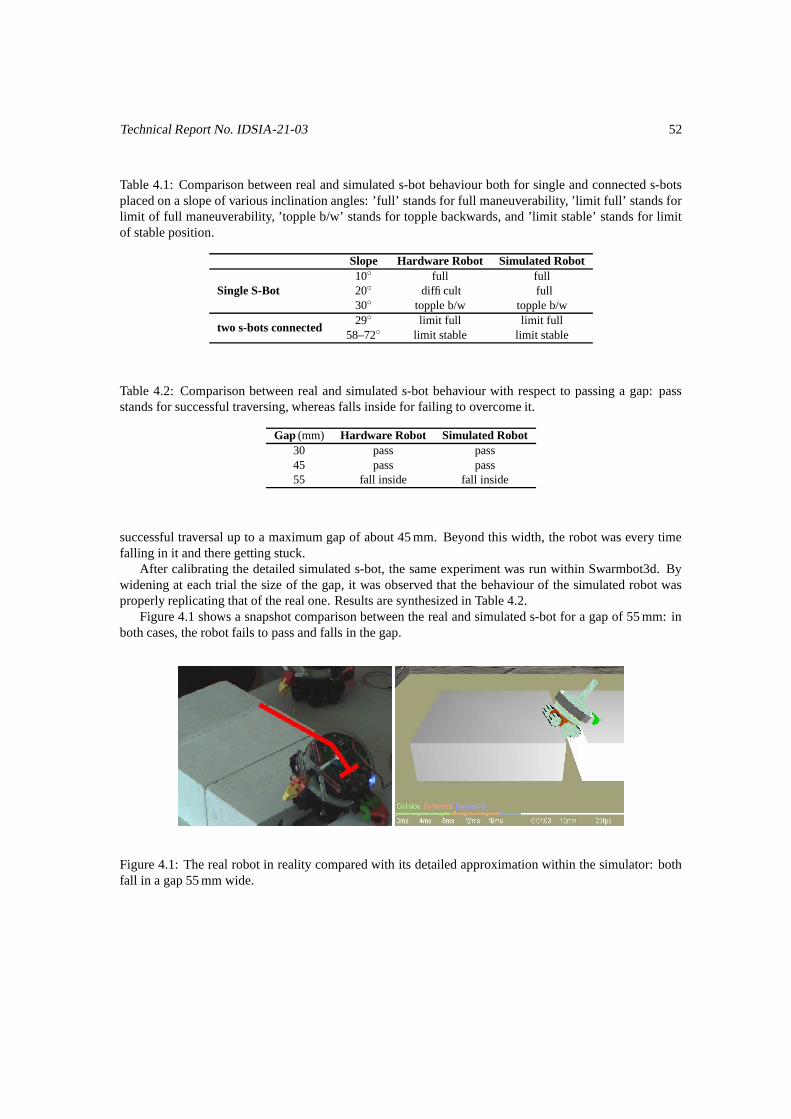
Technical Report No. IDSIA-21-03 52
Table 4.1: Comparison between real and simulated s-bot behaviour both for single and connected s-botsplaced on a slope of various inclination angles: ’full’ stands for full maneuverability, ’limit full’ stands forlimit of full maneuverability, ’topple b/w’ stands for topple backwards, and ’limit stable’ stands for limitof stable position.
Slope Hardware Robot Simulated Robot
Single S-Bot10◦ full full20◦ difficult full30◦ topple b/w topple b/w
two s-bots connected29◦ limit full limit full
58–72◦ limit stable limit stable
Table 4.2: Comparison between real and simulated s-bot behaviour with respect to passing a gap: passstands for successful traversing, whereas falls inside for failing to overcome it.
Gap (mm) Hardware Robot Simulated Robot30 pass pass45 pass pass55 fall inside fall inside
successful traversal up to a maximum gap of about 45 mm. Beyond this width, the robot was every timefalling in it and there getting stuck.
After calibrating the detailed simulated s-bot, the same experiment was run within Swarmbot3d. Bywidening at each trial the size of the gap, it was observed that the behaviour of the simulated robot wasproperly replicating that of the real one. Results are synthesized in Table 4.2.
Figure 4.1 shows a snapshot comparison between the real and simulated s-bot for a gap of 55 mm: inboth cases, the robot fails to pass and falls in the gap.
Figure 4.1: The real robot in reality compared with its detailed approximation within the simulator: bothfall in a gap 55 mm wide.

Technical Report No. IDSIA-21-03 53
Table 4.3: Maximum step climbing width for one single s-bot going backward and forward.
step height (mm)simulated s-bot real s-bot
backward forward backward forward≤ 15 pass pass pass pass16 fail ” fail ”23 ” ” ” ”24 ” fail ” fail
Figure 4.2: Equivalent behaviour of simulated and real s-bot with respect to a step size of 32 mm.
4.1.3 Real vs. Simulated Step Climbing
This experiment was set up in order to calibrate the behaviour of one simulated s-bot with that of the realone with respect to the task of climbing a step.
The step climbing experiment was split in two different parts: the first one calibrates a single s-bot,whereas the second one calibrates two s-bots connected in a chain.
Single S-Bot
One robot was placed close to a step and then moved towards it. The operation was carried out with bothforward and backward motion. Each time the test was performed, the step height was increased of 5 mm.
At the end of this sequence of tests, it emerged that the maximum step size which a single s-bot wasable to cope with was 15 mm going backward and 23 mm going forward (Table 4.3).
The difference between the two behaviours both in the simulated robot and in the real one is due to thecenter of mass of the turret which is 4 cm off centered towards the gripper. The reason for this stems fromthe mass of the gripper motors which are placed right behind it. It is in any case interesting to notice thatboth simulated and real s-bots produce equivalent response.
Figure 4.2 shows that at a step of 32 mm, which is the height at which two connected robot can pass(see next section), one single s-bot going backward topples over both in the simulated world and in reality.
Two Connected S-Bots with Gripper
The second part of the step passing experiment was carried out with two s-bots connected in a chain. To dothis, two disconnected s-bots were first placed one after the other along an orthogonal direction with respect

Technical Report No. IDSIA-21-03 54
Figure 4.3: From left to right: the different phases of the step passing for the limit step of 32 mm. Thepictures on the first column refer to the simulated s-bot and those on the second column to the actual s-bots.

Technical Report No. IDSIA-21-03 55
Table 4.4: Comparison of features among Fast, Simple, Medium, and Detailed s-bot simulation models.Yes and no respectively indicate the presence or absence of a particular feature in the model.
Model Fast1 Simple Medium Detaileddriving wheels # 2 2 6 6IR proximity sensors yes2 yes2 yes yesground sensors no no yes yescamera no no yes yessound module yes2 yes2 yes yesfront gripper no3 no3 yes4 yesflexible side arm no no no yesdynamical bodies # 6 6 8 23typical RTM 9501 94 31 3time step 1001 10 10 10
1) Measurement taken with 1/50th of gravity and 1/20th of mass.2) Using sample-based look-up table.3) No physical gripper model: connections are possible using virtual links.4) Coarse version, i.e. sticking box.
to the step, and then let them connect and move backward towards the step. By varying the height of thestep at each climbing, it was observed that the two robots were able to overcome up to 32 mm, exactly inaccordance with what experienced with the real s-bot.
Figure 4.3 shows four stages in passing the limit step of 32 mm. First, the two s-bots approach the stepin backward formation. Second, as soon as the first robot senses the step with its back-facing ground sensor,it starts lifting itself using its connected front gripper arm. During traversal, the robot bends its gripper armin opposite direction (downward) pushing itself up. Finally, the first robot continues its backward motionand pulls in this way the second one over the step to complete the procedure.
4.2 S-Bot Abstraction Evaluation
This section evaluates the different abstraction levels available for representing one simulated s-bot. Thesedifferent approximations (Fast, Simple, Medium, and Detailed) are ordered in an increasing level of refine-ment.
4.2.1 Efficiency Tests
The first test reported here establishes the computational overheads introduced by the use of a specificabstraction. Table 4.4 summarizes the differences among the models tested with a single s-bot on a flatplane. These results are indicated in Real Time Multiplier (RTM) values which represent how fast realtime can be simulated (e.g., RTM = 100 means that a simulation is 100 times faster than real time). RTMvalues depend, of course, on the available computing hardware; specifically the tests reported below werecarried out on a dual 3.06GHz Xeon PC with one nVidia QuadroFx 1000 graphics card.
4.2.2 Hierarchical Models’ Comparison Tests
The second series of tests reported in this section shows how the various s-bot abstractions compare withthe Detailed model which is used as a reference, given its established calibration with the real robot.

Technical Report No. IDSIA-21-03 56
Figure 4.4: Comparison of linear motion errors of the three s-bot simulation models with respect to differentterrain roughness.
Motion Comparison
This experiment compares how different models differ during forward linear motion on terrains with dif-ferent levels of roughness. To do so, each simulation model was placed randomly on a terrain and thenassigned a random heading. The terrain roughness was controlled within the simulator by specifying aheight range (HR) parameter. The HR values correspond to descriptive values: 1 for almost flat, 2 forminimally rough, 4 for little rough, 8 for mildly rough, 16 for rough, and 32 for very rough.
Given the reduced size of the Fast model, the terrain used for that s-bot abstraction was scaled down byhalf from its original size in order to retain comparable conditions.
Figure 4.4 shows the motion errors which are obtained by letting each s-bot model run at mediumspeed (15.24 cm/s) for 10 seconds. The vertical axis plots the projection of the travelled distance onto therandomly selected initial direction. Depending on the terrain roughness this distance decreases becausethe s-bot is not able to retain a straight course. The small differences in distance on flat terrain are causedby calibration errors of the velocity due to differences in the wheel diameter among the various s-botapproximations.
Figure 4.4 shows that the rough terrain motion of the Medium model closely follows the behaviour ofthe Detailed s-bot model: the constant offset is due to differences in wheel size (see above). Both Simpleand Fast models quickly fail to retain linear motion even on minimally rough terrains. Since the Detailedmodel replicates quite closely the behaviour observed on the real robot, this suggest that also the Mediumone can reasonably approximate it, at least as far as pure locomotion on rough terrain is concerned. TheFast and Simple Models should not be used for experiments using rough terrain.
4.2.3 Gap Passing
This particular experiment examines the problem of gap passing (Figure 4.5). The various s-bot approxi-mations are compared with the detailed one, which, given its close similarity with the real robot, is usedalso in this case as a reference.
The gaps are defined by means of two planar surfaces placed at a given distance. Table 4.5 summarizes

Technical Report No. IDSIA-21-03 57
Figure 4.5: From left to right, and from top to bottom: the 3 s-bot models while traversing a gap of 8, 9, 40and 60mm, respectively.

Technical Report No. IDSIA-21-03 58
Table 4.5: Gap passing comparison of the four s-bot approximations used.
Gap (cm) Fast Simple Medium Detailed3.0 pass pass pass pass4.0 “ “ “ “
4.5 “pass (70%) pass (90%)
“stuck (30%) stuck (10%)
5.0 “ stuck stuck “
5.7 “ “ “pass (50%)stuck (50%)
6.0 “ “ “ “6.5 stuck “ “ “
the tests obtained by varying the size of such a gap. Each table entry corresponds to the modal value of 12observations. All experimental tests were carried out by using a low speed of 2.8 cm/s in order to excludeeffects from finite inertia, i.e. that the robot would pass the gap merely due to a high speed.
4.2.4 Slope Tackling
This experiment reports how the various s-bot models compare when they encounter a slope (Figure 4.6).The navigation skills of the detailed model are once again used as a reference.
To quantify how the 4 models behave with respect to a sudden change in the evenness of the ground,three simulated s-bots, each expressed at a different level of refinement (Detailed, Medium, and Simple),were placed on a plane and then let them move forward until an uphill slope was encountered. The fastmodel had to be tested separately and alone, since it was meant to run in an environment with 1/50th ofgravity pull and with a time step 10 times higher (100ms).
The ability of each s-bot model to cope with a slope was observed as soon as each of them encountereda variation in the ground.
The maximum tilting angle each model was able to cope with was measured by progressively changingthe inclination angle of the slope with respect to the ground plane. The speed of all s-bots was also in thiscase set to 2.8 cm/s for the same reason pointed out in the gap passing experiment. Results are summarizedin Table 4.6: each entry corresponds to the modal value of 12 observations.
Downhill slopes are much less of a problem, since gravity, by forcing contact between s-bots andground, provides a mechanical aid to the motion. All models, in fact, successfully managed this type ofhindrance test up to about 0.5 radians. When slopes become steeper, all s-bots topple forward exactly asthe real robot does.
4.3 Simulation of Navigation on Composite Terrain using DynamicModel Switching
The aim of this experiment is to show a practical use of the hierarchy of models representing one s-bot.The problem considered here is the navigation of a single s-bot onto a complex terrain presenting differentlevels of difficulty in different stages. The hurdles are represented by three gaps, one slope, and two ruggedareas.
For this experiment, a variant of the Simple Model, called Basic Model, is introduced. This modeldiffer from the Simple one in the following points: (a) presence of a magnetic-like sticking device similarto that available for the Medium model, (b) ray traced IR sensors, (c) offset center of mass matching that

Technical Report No. IDSIA-21-03 59
Figure 4.6: From left to right: the 3 s-bots models tested for upward slope with inclination angle 0.1, 0.2,0.8 and 1.0 radians, respectively.
Table 4.6: Slope climbing comparison of the three s-bot approximations used: ’climb’ stands for successfulclimb, ’c/c’ stands for change course at the foot of the slope, and ’topple’ means the s-bot toppled overbackwards.
Angle (rad) Fast1 Simple medium detailed0.02 climb2 climb3 climb climb
0.04 “stuck (60%)
“ “c/c (40%)
0.20 c/c stuck climb climb0.70 “ “ “ “0.80 topple “ slipping slipping0.90 topple “ slide back topple1.00 stuck “ topple topple
1) Measurement taken in low gravity environment and with a high time step.2) Slope is overcome but course is changed slightly.3) Slope is taken but the initial direction is lost: s-bot changes course randomly.

Technical Report No. IDSIA-21-03 60
of the higher level approximations, and finally (d) a more accurately calibrated treels system. The intentionis to use the Basic model instead of the Simple one in future experiments involving connected swarmconfigurations. The characteristics of this model allow it to replace quite well the Medium and DetailedModels on the fly, that is during a simulation [8].
The simulation of this task is first carried out using the Detailed Model and then repeated using a tech-nique of dynamic model exchange. Such a simulation technique consists in letting one s-bot navigate alonga path and in switching its model representation on-the-fly according to the kind of terrain encountered(Figure 4.7).
The simulation starts with the Basic model on a flat plane. As long as the s-bot moves on flat ground,this simple robot representation is retained. As soon as a harder terrain is encountered (e.g., smaller gaps upto 5 cm, a slope, or medium rough terrain), the representation is switched to the Medium model. When alsothis one is not sufficient anymore (e.g., gaps larger than 5 cm, or very rough terrain situations), the Detailedmodel description is then used. As soon as a smooth plane is detected again, the simulator switches s-botrepresentation back to the Basic model, and so on. The gain obtained using the model changing techniqueis expressed as a reduction of total simulation time.
The diagram at the top in Figure 4.8 plots the aforementioned complex path followed by the detailedmodel repeated 10 times. The diagram at the bottom in the same figure plots the same path carried outusing the model switching technique. The two plots show that using model switching the simulated robotreaches the final position of the detailed robot within an acceptable range. It can be observed that thedetailed model is not very accurate in making right angle turns due to occasional slipping of the teethedwheels. The other two models do not have this problem, thus the plots using model switching show a morecompact clustering.
The simulated real time for completing complex navigation task was 59 real world seconds. The totalsimulation time required using the detailed model alone was about 64 seconds, whereas using the modelswitching technique was less than 28 seconds. This means that using model switching allows to reducesimulation time by more than half.
It should be pointed out, however, that any gain using the technique presented here is obviously depen-dent on the combination of terrain types. In the example discussed above, the more the environment allowsto use the simpler models, the more gain is expected in terms of simulation time.

Technical Report No. IDSIA-21-03 61
(a) (b)
(c) (d)
(e) (f)
(g) (h)
Figure 4.7: Simulation of one s-bot navigating onto different terrains while switching its model representa-tion. (a) The simulation starts with the Simple model; (b) at the trench the model switches to the Medium;(c) right after the trench it switches back to Simple; (d) just before the slope the switch from Simple, (e) toMedium; (f) on the slope the Medium representation; (g) switch to Detailed at the large trench; (h) remainDetailed on the rough terrain.

Technical Report No. IDSIA-21-03 62
Figure 4.8: Tracked path of the simulation using just the detailed s-bot model (top) and that of the simula-tion using the model switching technique (bottom).

Technical Report No. IDSIA-21-03 63
Acknowledgments
The work presented here is part of the SWARM-BOTS project, which is funded by the Future and EmergingTechnologies programme (IST-FET) of the European Community under grant IST-2000-31010 and by theSwiss Government under grant 01.0012.
The information provided is the sole responsibility of the authors and does not reflect the Community’sopinion. The Community is not responsible for any use that might be made of data published here.

Bibliography
[1] G. Baldassarre, S. Nolfi, and D. Parisi. Evolving mobile robots able to display collective behaviour.Artificial Life, 9:255–267, 2003.
[2] Luiz Chaimowicz, Mario Campos, and Vijay Kumar. Simulating Loosely and Tightly Coupled Multi-Robot Cooperation. In Anais do V Simposio Brasileiro de Automacao Inteligente (SBAI), Canela, RS,Brazil, September 2001.
[3] Bob Diamond. Concepts of Modeling and Simulation. http://www.imaginethatinc.com/pages/sim concepts paper.html,2002.
[4] H. Lund, E. Cuenca, and J. Hallam. A Simple Real-Time Mobile Robot Tracking System. TechnicalPaper 41, Department of Artificial Intelligence, University of Edinburgh, 1996.
[5] O. Michel. Webots: Symbiosis between Virtual and Real Mobile Robots. In Proceedings of the FirstInternational Conference on Virtual Worlds, VW’98, pages 254–263, Paris, France, 1998. SpringerVerlag.
[6] N. Minar, R. Burkhart, C. Langton, and M. Askenazi. The Swarm Simulation System, a Toolkit forBuilding Multi-Agent Simulations, 1996.
[7] Francesco Mondada, Giovanni C. Pettinaro, Andre Guignard, Ivo W. Kwee, Dario Floreano, Jean-Louis Deneubourg, Stefano Nolfi, Luca Maria Gambardella, and Marco Dorigo. SWARM-BOT: aNew Distributed Concept. Autonomous Robots, 2003. To appear soon.
[8] Giovanni C. Pettinaro, Ivo W. Kwee, and Luca M. Gambardella. Acceleration of 3D Dynamics Sim-ulation of S-Bot Mobile Robots using Multi-Level Model Switching. In Submitted to the IEEE Inter-national Conference on Robotics and Automation (ICRA ’04), New Orleans, Louisiana, U.S.A., 26thApril–1st May 2004.
[9] Giovanni C. Pettinaro, Ivo W. Kwee, Luca M. Gambardella, Francesco Mondada, Dario Floreano,Stefano Nolfi, Jean-Louis Deneubourg, and Marco Dorigo. Swarm Robotics: a Different Approach toService Robotics. In Proceedings of the 33rd International Symposium on Robotics (ISR ’02), pages71–76, Stockholm, Sweden, 7th–11th October 2002.
64

Appendix A
Standard S-Bot API
/*sbot.h : c interface to the s-bot robot(c) 2003 Stephane Magnenat, LSA 2, EPFL, SwarmBot Project*/
#ifndef __SBOT_H#define __SBOT_H
/* Set up for C function definitions, even when using C++ */#ifdef __cplusplusextern "C" {#endif
/** Sample sensor 50 times per second (50 Hz) */#define SAMPLING_RATE_50 1/** Sample sensor 33 times per second (33 Hz) */#define SAMPLING_RATE_33 2/** Sample sensor 20 times per second (20 Hz) */#define SAMPLING_RATE_20 3/** Sample sensor 10 times per second (10 Hz) */#define SAMPLING_RATE_10 4/** Sample sensor 5 times per second (5 Hz) */#define SAMPLING_RATE_5 5/** Sample sensor 2 times per second (2 Hz) */#define SAMPLING_RATE_2 6/** Sample sensor one time per second (1 Hz) */#define SAMPLING_RATE_1 7/** Sample sensor every two seconds (0.5 Hz) */#define SAMPLING_RATE_0_5 8
/** The sampling rate. Can take values SAMPLING_RATE_xx */typedef unsigned SamplingRate;
/** Do not blink leds*/#define BLINKING_RATE_NO_BLINK 0/** Blink leds 10 times per second (10 Hz) */#define BLINKING_RATE_10 1/** Blink leds 5 times per second (5 Hz) */#define BLINKING_RATE_5 2/** Blink leds 3.3 times per second (3.3 Hz) */#define BLINKING_RATE_3_3 3/** Blink leds 2.5 times per second (2.5 Hz) */#define BLINKING_RATE_2_5 4/** Blink leds 2 times per second (2 Hz) */#define BLINKING_RATE_2 5/** Blink leds one time per second (1 Hz) */#define BLINKING_RATE_1 6/** Blink leds every two seconds (0.5 Hz) */
65

Technical Report No. IDSIA-21-03 66
#define BLINKING_RATE_0_5 7/** Blink leds every three seconds (0.33 Hz) */#define BLINKING_RATE_0_33 8/** Blink leds every four seconds (0.25 Hz) */#define BLINKING_RATE_0_25 9/** Blink leds every five seconds (0.2 Hz) */#define BLINKING_RATE_0_2 10
/** The blink rate. Can take values BLINKING_RATE_xx */typedef unsigned BlinkingRate;
/** Initialize the s-bot. Request I2C low level interface and setdefault values. This function takes two arguments : they arethe callback function when an error (critical problem) or awarning (non-critical problem) is encountered.
\param errorHandler a pointer to the error function whichtakes the string describing the error in argument.
\param warningHandler a pointer to the warning function whichtakes the string describing the error in argument.*/void initSwarmBot(void (*errorHandler)(const char *errorString),void (*warningHandler)(const char *warningString));
/** Shutdown the s-bot. This function free the low level interfaces to I2C */void shutdownSwarmBot(void);
/** Set the speed of the tracks.\param left Left motor speed. [-127;127]\param right Right motor speed. [-127;127]*/void setSpeed(int left, int right);
/** Read the speed of the tracks.\param left Left motor speed pointer. [-127;127]\param right Right motor speed pointer. [-127;127]*/void getSpeed(int *left, int *right);
/** Read the torque of the tracks.\param left Left track torque pointer. [-127;127]\param right Right track torque pointer. [-127;127]*/void getTrackTorque(int *left, int *right);
/** Set the rotation angle of the turret.\param pos Angle of rotation. +/- 0.75 turn. [-100;100]*/void setTurretRotation(int pos);
/** Read the rotation angle of the turret.\return Angle of rotation. +/- 0.75 turn. [-100;100]*/int getTurretRotation(void);
/** Read the rotation torque of the turret.\return pos Torque on turret rotation motor. [-127;127]*/int getTurretRotationTorque(void);

Technical Report No. IDSIA-21-03 67
/** Set the elevation of the gripper.\param elevation Angle of elevation in degree. [-90;90]*/void setGripperElevation(int elevation);
/** Read the elevation of the gripper.\return Angle of elevation in degree. [-90;90]*/int getGripperElevation(void);
/** Set the aperture of the gripper.\param aperture Angle of aperture in degree. [0;40]*/void setGripperAperture(int aperture);
/** Read the aperture of the gripper.\return Angle of aperture of the gripper in degree. [0;40]*/int getGripperAperture(void);
/** Read the torque of the gripper.\return Angler of aperture of the gripper in degree. [-127;127]*/int getGripperElevationTorque(void);
/** Read the optical barrier of the gripper.\param internal Internal barrier pointer. 0 is obstructed, ˜700 is empty. [0;700]\param external External barrier pointer. 0 is obstructed, ˜700 is empty. [0;700]\param combined Combined barrier pointer. 0 is obstructed, ˜700 is empty. [0;700]*/void getGripperOpticalBarrier(unsigned *internal, unsigned *external,
unsigned *combined);
/** To be measured */void setSideArmPos(int elevation, int rotation, int depth);
/** To be measured */void getSideArmPos(int *elevation, int *rotation, int *depth);
/** To be measured */void getSideArmTorque(int *elevation, int *rotation, int *depth);
/** Fully open the side-arm’s gripper. */void setSideArmOpened(void);
/** Fully close the side-arm’s gripper. */void setSideArmClosed(void);
/** Read the optical barrier of the side arm.\param internal Internal barrier pointer. 0 is obstructed, ˜700 is empty.[0;700]\param external External barrier pointer. 0 is obstructed, ˜700 is empty.[0;700]\param combined Combined barrier pointer. 0 is obstructed, ˜700 is empty.[0;700]*/void getSideArmOpticalBarrier(unsigned *internal, unsigned *external,
unsigned *combined);
/** Read the value of a proximity sensor.\param sensor Number of sensor. [0;14]\return Distance to object. 20 is 15 cm, 50 is 5 cm, 1000 is 1 cm, 3700is 0.5 cm. [0;8191]*/unsigned getProximitySensor(unsigned sensor);

Technical Report No. IDSIA-21-03 68
/** Read the value of all proximity sensors.\param sensors Array of distances to objects. For each value, 20 is 15 cm,50 is 5 cm, 1000 is 1 cm, 3700 is 0.5 cm. [0;8191]*/void getAllProximitySensors(unsigned sensors[15]);
/** Set the sampling rate of the proximity sensors.\param rate Sampling rate. Can take values SAMPLING_RATE_xx.*/void setProximitySamplingRate(SamplingRate rate);
/** Read the value of a ground sensor.\param sensor Number of sensor. [0;3]\return Distance to object. 1 is 6mm, 25 is 2mm, 100 is 1mm. [0;255]*/unsigned getGroundSensor(unsigned sensor);
/** Read the value of all ground sensors.\param sensors Array of distances to objects. For each value, 1 is 6mm,25 is 2mm, 100 is 1mm. [0;255]*/void getAllGroundSensors(unsigned sensors[4]);
/** Set the sampling rate of the ground sensors.\param rate Sampling rate. Can take values SAMPLING_RATE_xx.*/void setGroundSamplingRate(SamplingRate rate);
/** Read the value of a light sensor.\param sensor Number of sensor. [0;7]\return Intensity. 0 is full dark, ˜700 is full light.[0;700]*/unsigned getLightSensor(unsigned sensor);
/** Read the value of all light sensors.\return Array of intensities. For each value, 0 is full dark, ˜700 is fulllight. [0;700]*/void getAllLightSensors(unsigned sensors[8]);
/** Set the color of a light.\param light Number of light. [0;7]\param r Red intensity. [0;15]\param g Green intensity. [0;15]\param b Blue intensity. [0;15]\param blink Blinking rate. Can take values BLINKING_RATE_xx.*/void setLightColor(unsigned light, unsigned r, unsigned g, unsigned b,
BlinkingRate blink);
/** Set the color of all lights.\param r Array of red intensities. For each value [0;15]\param g Array of green intensities. For each value[0;15]\param b Array of blue intensities. For each value [0;15]\param blink Array of blinking rates. For each value, can take valuesBLINKING_RATE_xx.*/void setAllLightColor(unsigned r[8], unsigned g[8], unsigned b[8],
BlinkingRate blink[8]);
/** Set the same color for all lights.\param r Red intensity. [0;15]\param g Green intensity. [0;15]

Technical Report No. IDSIA-21-03 69
\param b Blue intensity. [0;15]\param blink Blinking rate. Can take values BLINKING_RATE_xx.*/void setSameLightColor(unsigned r, unsigned g, unsigned b, BlinkingRate blink);
/** Set the sampling rate of the light sensors.\param rate Sampling rate. Can take values SAMPLING_RATE_xx.*/void setLightSamplingRate(SamplingRate rate);
/** Read the left temperature and humditiy sensor.\param temperature Temperature in degree pointer. [-40;123]\param humidity Relative humidity in % pointer. [0;100]*/void getTemperatureAndHumidityLeft(float *temperature, float *humidity);
/** Read the right temperature and humditiy sensor.\param temperature Temperature in degree pointer. [-40;123]\param humidity Relative humidity in % pointer. [0;100]*/void getTemperatureAndHumidityRight(float *temperature, float *humidity);
/** Read the slope pitch & roll angles of the robot\param pitch Pitch in degree pointer. [-180;180]\param roll Roll in degree pointer. [-180;180]*/void getSlope(int *pitch, int *roll);
/** Set the sampling rate of the slope sensor.\param rate Sampling rate. Can take values SAMPLING_RATE_xx.*/void setSlopeSamplingRate(SamplingRate rate);
/** Read the current battery voltage\return Return the current battery voltage 0-10V [0;255]*/unsigned getBatteryVoltage(void);
/*TODO :- v4l abstraction for camera*/
/** TO BE DEFINED */void playMusic(const char *filename);
/** TO BE DEFINED */void stopMusic(void);
/* Ends C function definitions when using C++ */#ifdef __cplusplus}#endif
#endif

Appendix B
Class Diagrams
This appendix presents UML class diagrams of the main modules of the Swarmbot3dsimulator software.
70

Technical Report No. IDSIA-21-03 71
Figure B.1: Class diagram of TreelsModule and related classes.

Technical Report No. IDSIA-21-03 72
Figure B.2: Class diagram of TurretModule and related classes.

Technical Report No. IDSIA-21-03 73
Figure B.3: Class diagram of GripperModule and related classes.

Technical Report No. IDSIA-21-03 74
Figure B.4: Class diagram of LightRingModule and related classes.

Technical Report No. IDSIA-21-03 75
Figure B.5: Class diagram of ProximitySensorModule and related classes.

Technical Report No. IDSIA-21-03 76
Figure B.6: Class diagram of CameraModule and related classes.

Technical Report No. IDSIA-21-03 77
Figure B.7: Class diagram of SideArmModule and related classes.
Figure B.8: Class diagram of SoundModule and related classes.

Technical Report No. IDSIA-21-03 78
Figure B.9: Class diagram of SBot and related classes.

Technical Report No. IDSIA-21-03 79
Figure B.10: Class diagram of VortexWorld and related classes.