design and concrete material requirements for ultra …

DESIGN AND CONCRETE MATERIAL REQUIREMENTS FOR ULTRA-THIN

WHITETOPPING

Prepared By

Jeffery Roesler Amanda Bordelon

University of Illinois at Urbana-Champaign

Anastasios Ioannides University of Cincinnati

Matthew Beyer

Dong Wang University of Illinois at Urbana-Champaign

Research Report FHWA-ICT-08-016

A report of the findings of

IHR-R27-3A Design and Concrete Material Requirements for Ultra-Thin Whitetopping

Illinois Center for Transportation

June 2008

CIVIL ENGINEERING STUDIES Illinois Center for Transportation Series No. 08-016

UILU-ENG-2008-2003 ISSN: 0197-9191

Technical Report Documentation Page 1. Report No.

FHWA-ICT-08-016

2. Government Accession No. 3. Recipient's Catalog No.

4. Title and Subtitle 5. Report Date

June 2008

DESIGN AND CONCRETE MATERIAL REQUIREMENTS FOR ULTRA-THIN WHITETOPPING

6. Performing Organization Code

8. Performing Organization Report N o. 7. Author(s)

J. Roesler, A. Bordelon, A. Ioannides, M. Beyer, D. Wang

FHWA-ICT-08-016 UILU-ENG-2008-2003

9. Performing Organization Name and Address 10. Work Unit ( TRAIS)

University of Illinois at Urbana Champaign 205 North Mathews Ave. – MC 250

11. Contract or Grant No.

Urbana, Illinois 61866

13. Type of Report and Period Covered

12. Sponsoring Agency Name and Address

Illinois Center for Transportation University of Illinois at Urbana Champaign 1611 Titan Drive Rantoul, Illinois 61866

14. Sponsoring Agency Code

15. Supplementary Notes

16. Abstract

The objectives of this research were to provide the Illinois Department of Transportation (IDOT) with an ultra-thin whitetopping (UTW) thickness design method and guidelines for UTW design, concrete material selection, and construction practices. A new mechanistic-empirical design method was proposed based on a modified version of the American Concrete Pavement Association (ACPA) design method for UTW. This proposed guide calculates the required UTW thickness based on traffic level, pavement layer geometry, climate, materials, and the pre-existing HMA condition. Laboratory testing of UTW concrete mixtures suggested many proportions and constituents can be successfully used as long as consideration is made to minimize the concrete’s drying shrinkage (e.g., limited cement content) and maintain the concrete- HMA bond.

The laboratory testing coupled with previous fiber-reinforced concrete (FRC) slab tests suggested that structural fibers should be utilized in future UTW projects in order to reduce the required slab thickness without increasing the concrete strength, limit the crack width, expand the required slab size, and to extend the functional service life of fractured slabs and potentially extend the performance of non-reinforced concrete joints. A residual strength ratio ( 150

150R ) was proposed to characterize the performance of any FRC mixture to be used in UTW systems. This residual strength ratio can be calculated based on measured parameters from ASTM C 1609-07 and has been incorporated into the design guide to account for the structural benefits of using FRC. Finally, recommendations for saw-cut timing and construction techniques are also presented in this report.

17. Key Words

Pavement, ultra-thin whitetopping, fibers, design

18. Distribution Statement

No restrictions. This document is available to the public through the National Technical Information Service, Springfield, Virginia 22161.

19. Security Classif. (of this report)

Unclassified

20. Security Classif. (of this page)

Unclassified

21. No. of Pages

22. Price

Form DOT F 1700.7 (8-72) Reproduction of completed page authorized

i

ACKNOWLEDGMENT This publication is based on the results of ICT-R27-3A Design and Concrete Material Requirements for Ultra-Thin Whitetopping. ICT-R27-3A was conducted in cooperation with the Illinois Center for Transportation; the Illinois Department of Transportation, Division of Highways; and the U.S. Department of Transportation, Federal Highway Administration.

Members of the Technical Review Panel are: James Krstulovich, IDOT (TRP Chair) Kevin Burke, IDOT Doug Dirks, IDOT Mark Gawedzinski, IDOT Scott Lackey, IDOT Dave Lippert, IDOT Dan Tobias, IDOT Tom Winkelman, formerly of IDOT Randell Riley, ACPA DISCLAIMER

The contents of this report reflect the view of the author(s), who is (are) responsible for the facts and the accuracy of the data presented herein. The contents do not necessarily reflect the official views or policies of the Illinois Center for Transportation, the Illinois Department of Transportation, or the Federal Highway Administration. This report does not constitute a standard, specification, or regulation.

ii

EXECUTIVE SUMMARY

The objectives of this research were to provide the Illinois Department of Transportation (IDOT) with an ultra-thin whitetopping (UTW) thickness design method and guidelines for UTW design, concrete material selection, and construction practices. During this study, existing UTW projects were reviewed with the focus on the concrete mixture designs and field distress data to assist in generating an optimal state-of-the-art design method. The UTW projects studied that had premature distresses were typically thin or highly distressed hot mix asphalt (HMA) sections and high cement content mixtures. In order to evaluate the in-situ properties of UTW, falling weight deflectometer (FWD) tests were performed on some of the projects. Due to the variability in the HMA thickness and stiffness, unbound material support layers, and UTW slab size, back-calculation of the layer properties was difficult and was not included at this time. However, FWD testing allowed for an in-depth look at the joint load transfer efficiency and was an indicator of the concrete-HMA bond condition and the condition of the UTW support layers.

A new mechanistic-empirical design method was proposed based on a modified version of the American Concrete Pavement Association (ACPA) design method for UTW. This proposed guide calculates the required UTW thickness based on traffic level, pavement layer geometry, climate, materials, and the pre-existing HMA condition. Laboratory testing of UTW concrete mixtures suggested many proportions and constituents can be successfully used as long as consideration is made to minimize the concrete’s drying shrinkage (e.g., limited cement content) and maintain the concrete- HMA bond.

The laboratory testing coupled with previous fiber-reinforced concrete (FRC) slab tests suggested that structural fibers should be utilized in future UTW projects in order to reduce the required slab thickness without increasing the concrete strength, limit the crack width, expand the required slab size, and to extend the functional service life of fractured slabs and potentially extend the performance of non-reinforced concrete joints. A residual strength ratio ( 150

150R ) was proposed to characterize the performance of any FRC mixture to be used in UTW systems. This residual strength ratio can be calculated based on measured parameters from ASTM C 1609-07 and has been incorporated into the design guide to account for the structural benefits of using FRC. Finally, recommendations for saw-cut timing and construction techniques are also presented in this report.

iii

CONTENTS Acknowledgment ............................................................................... i Disclaimer .......................................................................................... i Executive Summary ......................................................................... ii Chapter 1. Introduction .................................................................... 1 Chapter 2. Evaluation and Testing .................................................. 3 Chapter 3. Design Procedure ........................................................ 10 Chapter 4. Design Charts ............................................................... 25 Chapter 5. Design Tables ............................................................... 34 Chapter 6. Conclusions ................................................................. 36 Chapter 7. Recomendations .......................................................... 37 References ...................................................................................... 38 Appendix A. Existing UTW Pavement Condition ....................... A-1 Appendix B. FWD Deflection Results ......................................... B-1 Appendix C. Concrete Material Testing ...................................... C-1 Appendix D. Fiber-Reinforced Concrete Test Results .............. D-1 Appendix E. Past Design Guides ................................................. E-1 Appendix F. Thermal Stress Analysis ......................................... F-1

1

CHAPTER 1. INTRODUCTION

1.1 BACKGROUND

Ultra-thin whitetopping (UTW) is a concrete pavement overlay alternative to hot mix asphalt (HMA) overlay. UTW can be used to rehabilitate and extend the service life of existing HMA pavement structures which have failed from rutting, local surface distresses, fatigue cracking, and low-temperature cracking.

1.1.1 History of UTW Projects

Between 1918 and 1991, approximately 200 thin whitetopping (TWT) projects had been documented. Since 1991, the American Concrete Pavement Association (ACPA) has been tracking the use of UTW in the United States and has documented more than 300 additional projects during this period. The first UTW project in the United States was constructed in Louisville, Kentucky, in 1991 (Cole and Mohsen, 1993). The Louisville UTW consisted of two concrete thicknesses [2-in. (51-mm) and 3.5-in. (89-mm)] and two slab sizes [2 x 2 ft (0.6 x 0.6 m) and 4 x 4 ft (1.2 x 1.2 m)]. Since the Louisville project, the use of UTW and TWT has exhibited significant growth in the United States. Rehabilitation projects have been completed in many locations throughout the United States such as California, Colorado, Iowa, Florida, Louisiana, Kansas, Virginia, Missouri, Minnesota, New Jersey, Oklahoma, and Tennessee. The Illinois Department of Transportation (IDOT) has also experimented with whitetopping since 1974 and with UTW since 1998. An excellent summary of TWT and UTW basic design factors and pavement projects is provided in NCHRP Synthesis 338 (Rasmussen and Rozycki, 2004).

Other countries have also experimented with UTW and TWT. In 1993, Sweden constructed four test sections of TWT and evaluated their performance under heavy traffic for 18 months (Silfwerbrandt and Petersson, 1993). Mexico has constructed a UTW research project on an urban arterial in Tijuana (Salcedo 1998). Other countries reporting recent UTW projects include Brazil (Balbo 2003), in which six experimental sections of UTW employing high strength concrete were monitored until failure; Japan (Nishizawa et al. 2003), in which a test UTW pavement was constructed on a yard in a cement plant in 1999; and South Korea (Cho and Koo, 2003), where load tests were conducted in 2000. Based on studies such as these, it has been observed that for specific applications and service life requirements, well-designed and well-constructed UTW and TWT appear to provide satisfactory performance.

1.1.2 UTW Design

UTW has traditionally been defined to be within the range of 2 to 4 in. (51 to 102 mm) of concrete slab thickness (ACPA 1998). UTW consists of smaller slab sizes because of their high surface to volume ratio, and to reduce the moisture and temperature curling and load stresses on the surface of the concrete slabs. The exact thickness of the slab is dependent on the soil support layer, stiffness and thickness of the HMA support layer, bonding condition with the HMA, traffic level, concrete strength, and slab size. Many agencies and engineers designing UTW have used the ACPA procedure for the thickness determination (ACPA 1998).

The slab size, saw-cut timing, and bonding are important design parameters that must be addressed during construction of UTW pavements. The fracture properties of

2

the concrete mixture can be used to understand the mechanisms behind the UTW pavement performance, especially load carrying capacity, load transfer efficiency at joints, and how quickly the system may fail if it de-bonds from the existing HMA layer.

Currently no quantitative condition assessment of the existing HMA pavement exists and there are limited guidelines as to appropriate constituents and proportions in the concrete mixture designs required to assure adequate performance of this concrete overlay strategy.

1.2 OBJECTIVES

The objectives of this research project were to provide IDOT with an enhanced UTW thickness design method and guidelines for UTW design, concrete material selection, and construction practices specific to UTW. The specific tasks of this project are to evaluate the effects of fibers and concrete material properties on slab size and thickness requirements. Factors such as existing condition of the HMA, HMA thickness, interface preparation and strength, and saw-cut timing and depth will be evaluated and guidelines established. Existing procedures for UTW will be reviewed and a simple design tool to determine UTW thickness based on the concrete mixture design, traffic, and existing pavement conditions will be developed.

3

CHAPTER 2. EVALUATION AND TESTING

The majority of the IDOT UTW projects have been successful with minimal distresses such as cracked slabs (Winkelman 2005a and 2005b). However a few of the projects performed by IDOT demonstrated early-age distresses. Similarly, projects in Brazil and Taiwan (Balbo 2003; Lin and Wang, 2005) were found to have severely cracked slabs at early ages. It was discovered that the common factor in the early-age cracking occurred with mixtures which contained high cement contents or low water-cement ratios and possibly thin HMA support layer. Appendix A is a summary of the performance of UTW projects by IDOT, Brazil, and several projects monitored at the University of Illinois at Urbana-Champaign (UIUC) campus.

2.1 DISTRESS SURVEY SUMMARY

The primary distresses exhibited on the selected projects were corner breaks frequently but not always proceeded by areas of de-bonding, as described in Appendix A. The corner breaking being the primary distress supports the original UTW research assumptions that the critical stress location for design of the UTW thickness is the corner stress.

The design life of UTW has typically not been specified as in other facilities, such as highways, but only the allowable number of design ESALs. IDOT is targeting the service life of UTW to be 15 years. With this service life considered in the design, UTW sections should provide adequate functional service even with the occurrence of distresses, and should not be thought of as a failed section due to an appearance of a crack. UTW may require some maintenance throughout its service life, but overall it should provide functionality through its service life despite the existence of some level of structural distress.

The observation from distress surveys of field UTW sections in Illinois and in other countries has demonstrated that the existing condition of the HMA layer, bonding at the PCC/HMA interface, and concrete mixture proportions can affect the early-age performance of the UTW section. In projects with early-age failures, de-bonding of the concrete layer from the HMA layer occurred. In all cases studied herein, the concrete mixtures for these sections had significantly higher cement contents, resulting in more shrinkage that likely contributed to the potential for de-bonding at the PCC/HMA interface. In several of the failures found in projects around the world, thin HMA layers [less than 2-in. (51-mm)] were also a factor in development of early-age cracking, especially when high shrinkage mixtures were utilized.

2.2 FWD EVALUATION

Several UTW projects with IDOT and on the UIUC campus were tested using a falling weight deflectometer (FWD). Four sites in the state of Illinois, where FWD data was available, were analyzed and the details of the testing and analysis are presented in Appendix B. The specific projects tested with the FWD were the UIUC E-15 parking lot, Piatt County Highway 4, Tuscola US Highway 36, and the Schanck Avenue project near Chicago (Mundelein, IL).

4

2.2.1 FWD Drop Procedure

The initial intent of the FWD testing was to characterize the individual UTW system layers, joint load transfer efficiency (LTE), and stiffness of the existing distressed HMA layer. Five consecutive slabs were tested using the FWD for the IDOT projects; fifteen consecutive slabs were tested on the E-15 parking lot project. The joint performance was evaluated by comparing deflections on either side of the transverse joints with the theoretical performance of a continuous slab without joints (center slab case). To determine maximum load transfer efficiency, the deflection taken at a center slab drop was compared with the deflection at a 12-in. (302-mm) offset from the center. The load drops were at 6, 9, and 12 kips (27, 40, and 53 kN). Details on the drop procedure can be found in Appendix B. The structural capacity of the UTW system was assessed with the AREA and AUPP (Area Under Pavement Profile) parameters.

2.2.2 FWD Results

The FWD results were primarily used to assess the variation in surface deflections along the project and to characterize performance of the joints. In pavements where a strong support condition and good PCC/HMA interface bond existed, load transfer efficiency values were between 80 and 90 percent. UTW pavements where the structural condition of the underlying support layer is poor or deteriorated bond may have existed, the load transfer at the joint and center slab was significantly reduced. The IDOT project in Tuscola contained an asphalt overlay of a brick road which was already significantly distressed, and a smooth surface texture existed prior to the UTW. Therefore, the measured load transfer efficiency values for the UTW system after construction were lower for the Tuscola project. Another observation was that thin HMA layers [less than 2.5-in. (63.5-mm)] tended to crack full-depth when the concrete joint cracked. The load transfer at the locations of the full-depth crack through the concrete and HMA was significantly lower than other joints. Finally, it was difficult to assess if all joints had cracked in the field since LTE greater than 80 percent could indicate excellent support condition and bond or indicate that the crack had not propagated at that saw-cut location.

2.2.3 Existing HMA Backcalculation

FWD results were useful in providing information on how the joints were performing in the field, as well as information regarding variation in the support conditions. The deflections from the FWD can also be used to back-calculate the existing conditions (elastic modulus and thickness of the asphalt) of the existing pavement structure prior to placement of the UTW layer. Due to the limited FWD data that existed on the distressed HMA layer and uncertainty in the HMA layer stiffness and thickness, and the exact thickness of the UTW thickness, back-calculation of the individual layer properties was not successful. Furthermore, back-calculation procedures are based on the assumption that the slab size is large enough that infinite dimensions can be assumed, which is an invalid assumption with UTW systems. Thus, a mechanistic method to back-calculate the effective stiffness of the existing distressed HMA was not included in this research, but is of great interest for future work.

5

2.2.4 FWD Summary

The FWD testing has shown that a program to monitor UTW sections over time will be beneficial in determining the performance of the joints, interface bond condition, and the structural capacity of the section (condition of the HMA and underlying support layers). In the short term, the FWD program has demonstrated that not all saw-cut joints have propagated cracks through the slab. The use of early-entry saws must continue to be used to assure cracks are going to occur at regular intervals. With cracks every 20 to 30 ft (6 to 9 m) occurring initially in UTW sections, significant crack widths exist at these locations, which may result in the distress developing at these locations. An alternative technique to create joints rapidly and cost effectively at all saw-cut locations is advantageous. A technique to dynamically fracture the joints (Cockerell 2007) without damaging the slabs is one option that could reduce the joint formation cost and yet provide a superior performing joint over the long-term.

2.3 CONCRETE TESTING

With distresses in field pavement sections occurring where inadequate support, de-bonding, or high strength concrete mixtures existed, a laboratory study was performed to investigate the influence of the mixture design proportioning and constituents on potential UTW performance. In order to analyze the link between the performance of UTW field test sections in Illinois with the concrete materials used on the projects, laboratory testing was performed using the same mixture proportions as those described in Appendix A.

Beam fracture testing and composite beam testing was performed on the UTW mixtures to evaluate the concrete material performance before, during, and after cracking given a set of boundary conditions, loading configuration, and specimen geometry. Specifically, simply-supported notched three-point bend specimens and fully-supported composite beams (PCC and HMA) were cast and tested. Fresh property and strength tests were also performed on each mixture at different ages. These tests included slump, unit weight, air content, split tensile and compressive strength and drying shrinkage. A summary of the tests and significant findings are provided in this section.

2.3.1 Fracture Testing 2.3.1.1 Test Procedure

The fracture properties of the UTW concrete mixture are important to describe the concrete’s resistance to cracking and its potential service life in UTW applications, especially when the potential for de-bonding at the PCC/HMA interface exists or the old HMA surface exhibits cracking. A RILEM procedure developed by Jenq and Shah (1985) and Shah et al. (1995) using a single-edge notched beam [SEN(B)] was employed to determine the fracture properties of the concrete. Any improvement in the concrete mixture’s fracture properties was hypothesized to improve the cracking resistance of UTW or to extend the service life of the UTW. The SEN(B) is configured for three-point bending with the load (P) and crack mouth opening displacement (CMOD) being measured.

An analysis technique known as the Two-Parameter Fracture Model (TPFM) was used to determine initial fracture properties: the critical stress intensity factor (KIC) and

6

critical crack tip opening displacement (CTODC) of a beam based on an effective elastic crack approach. The initial fracture properties were calculated from the loading and unloading compliance, the peak load (Pc), the beam weight, and the initial notch depth. These initial fracture properties of the concrete predict the concrete resistance to crack initiation and crack growth.

The testing data from the SEN(B) concrete specimen can also be used to calculate the area under the load-CMOD curve which can be related to the concrete’s total fracture energy (GF) using the Hillerborg (1985) method. The total fracture energy is beneficial in assessing the total amount of work required to completely separate two concrete surfaces. Details on the geometry recommendations, testing procedure, and analysis methods can be found in Appendix C.

2.3.1.2 Age Effect of Fracture Test

Similar to strength testing, concrete fracture properties are dependent on age at testing. On average for all the mixtures tested, 75 percent of the fracture and strength properties were realized by 7 days, and 85 percent by 28 days. The initial fracture energy of the E-15 Parking Lot mixture containing fiber-reinforced concrete (FRC) doubled between 7 and 28 days. The total fracture energy of FRC increased almost seven times between 7 and 28 days, for the same mixture.

For the un-reinforced concrete mixtures, the total fracture energy did increase with age and ranged in values between 83 N/m to 141 N/m. Bazant and Becq-Giraudon (2002) determined in a statistical study for non-reinforced concrete that the coefficient of variability (COV) for initial and total fracture energy were on the order of 18 and 30 percent, respectively. It was determined that an age of 28 days would be more appropriate to use as a reference time since the COV after this point in time was reduced, and little change occurred between 28 and 90 days.

2.3.1.3 Mixture Design Parameters

A variety of materials and proportions can be used in UTW. The concrete material constituents and proportions selected should prevent premature de-bonding and increase the material’s fracture resistance so that the service life of the UTW can be maximized. FRC can offer fracture resistance, reflective crack resistance, and reduce the probability of immediate failure from de-bonding as compared to plain concrete. Using the SEN(B) test, the total fracture energy parameter can be used to emphasize the benefit of using FRC compared to plain concrete especially for establishing the load capacity of the concrete structure after cracking has occurred. The influence of FRC in terms of proportioning and toughness is described in a subsequent section.

The influence of aggregate type on fracture properties was investigated by comparing the crushed limestone primarily used with other coarse aggregates such as recycled concrete aggregate and river gravel. The quality of the coarse aggregate was linked to the strength and fracture properties of the concrete. With the river gravel coarse aggregate, the concrete was more brittle for the initial fracture properties, but the total fracture energy was greater after 28 days compared to concrete containing crushed limestone coarse aggregate. With at least 50 percent replacement with crushed limestone aggregate, the recycled coarse aggregate concrete specimens resulted in roughly the same fracture properties as virgin coarse aggregate concrete.

The choice in material proportioning can affect some of these hardened properties. For example, higher cement contents tend to increase shrinkage within the concrete, although it may also aid in increasing the compressive and tensile strength

7

and initial fracture energy of the concrete as well. The high cost of cement and the potential of the hydration products to shrink should be considered so that specifications minimize the amount of cement in the mixture. Cementitious contents for the studies shown in Appendix C ranged from approximately 560 to 808 lb/yd3 (332 to 479 kg/m3). No correlation was found between the total fracture energy and proportioning of cement or aggregates in this study.

2.3.2 Composite Beam Testing

Full-scale fiber-reinforced concrete (FRC) slabs have clearly demonstrated that fibers increase the flexural and ultimate load capacity of plain concrete slabs (Roesler et al. 2004; 2006), decrease the width of surface cracks, should provide reflective cracking resistance relative to plain concrete, and should extend the functional service life of distressed UTW. In order to further evaluate the efficacy of fibers in UTW concrete mixtures, a laboratory investigation of a two-dimensional composite beam specimen supported by a soil foundation was conducted. A comparison of seven selected IDOT mixture designs used in the UTW projects around the state of Illinois (see Appendix A) were replicated in the laboratory.

Through iterations on the geometry and set-up of the composite beam test, a finalized test was developed. This test was comprised of a concrete beam cast directly onto an aged asphalt beam (the asphalt beam was notched full-depth to represent a crack in the HMA) sitting on a clay soil foundation. The concrete specimen was loaded above the cracked asphalt to force a stress concentration in the concrete material. Details of the test setup and iterations for development of the composite beam test can be found in Appendix C.

The peak load capacity of the composite beam was closely linked to the compressive strength of the concrete. The immediate drop in post-peak load was estimated to represent the structural integrity of the UTW once a crack formed. The magnitude of the immediate load drop can be associated with the performance of UTW in the field after some initial cracking has occurred. Recent research predicted the load carrying capacity of slabs based on the equivalent flexural strength ratio ( 150

150R ) of fiber-reinforced concrete beams, which is based on the magnitude of the post-peak load drop (Altoubat et al. 2008). Similar to the poorer performance in the field, the Anna mixture showed a large drop in load (54 percent) after cracking in the composite beam test setup. On the other hand, the FRC mixtures containing 0.26 and 0.40 percent volume fraction of fiber-reinforcement had the two lowest load drops at 29 and 42 percent respectively. Further details of the composite beam test results are in Appendix C.

In summary, the composite beam tests demonstrated that fibers would enhance the performance of UTW especially in the post-crack initiation stage. This testing also demonstrated that higher strength mixtures can provide a higher peak load at failure as long as bond is maintained between the PCC/HMA interface. However, post-peak behavior of some higher strength mixtures could pose problems in the field (rapid loss in load carrying capacity) if cracking initiates from reflective cracking or as a result of de-bonding. Overall, the 2-D composite beam test still was not as effective as it was anticipated to be in terms of differentiating performance of various concrete mixtures. In the future, a limited set of full-scale UTW slabs with different concrete mixtures should be load tested to further verify the composite beam results.

8

2.3.3 Free Drying Shrinkage

Excessive concrete drying shrinkage can cause de-bonding between the concrete and existing asphalt pavement. Higher strength concrete mixtures were typically more susceptible to this behavior due to their higher total cementitious material content. After conducting laboratory shrinkage tests on selected UTW mixtures (see Appendix C), the Anna mixture containing the highest cement content of 755 lb/yd3 (448 kg/m3) and a low water cement ratio of 0.36 represented the greatest free drying shrinkage. The Schanck Avenue mixture containing fiber-reinforcement and 515 lb/yd3 (306 kg/m3) of cement, 140 lb/yd3 (83 kg/m3) fly ash, and water to cementitious ratio 0.41 had the lowest free drying shrinkage potential. Although the magnitude of the free shrinkage strains can indicate the potential for early-age cracking or de-bonding, it is also important to know the rate of its occurrence relative to the strength gain, the field curing conditions, and the shrinkage differential through concrete layer.

2.4 FIBER-REINFORCED CONCRETE (FRC) TESTING 2.4.1 Fiber Type

The following types of structural fibers were studied in the lab: straight synthetic, crimped synthetic, twisted synthetic, two hooked end steel, and two crimped steel fibers. Volume fractions ranging from 0.19 to 1.56 percent were studied for fracture and flexural strength properties. Appendix D describes the testing and properties found for the different FRC mixtures. The laboratory testing conducted in this research project and previous test results from other authors (Lange and Lee, 2005; Rieder 2002; Huntley 2007; Donovan and Strickler, 2007) determined the volume fraction or dosage rate cannot be used to predict the post-cracking performance of FRC materials. Testing must be performed to determine the exact performance of each fiber type and the respective dosage rate required for a given level of performance (e.g., equivalent flexural strength or toughness).

2.4.2 Test Methods

The 4-point bending flexure test (ASTM C 78)—modulus of rupture (MOR)— can be used to determine the peak strength of the concrete for various types and volume fractions of fibers. Three standard methods were evaluated to describe the post-peak performance or residual strength of FRC: ASTM C 1018, ASTM C 1609, and JCI-SF4. In addition, the fracture energy testing previously mentioned was performed on some of the fiber types to compare the post-peak residual performance with the total fracture energy.

The equivalent residual flexural strength ratio ( DR150 ) is computed as the ratio of the post-peak flexural strength of the FRC mixture ( Df150 ) at a given net deflection to the concrete MOR. The residual properties of each standard were compared and it was found the residual strength ratio obtained using the ASTM C 1609 method produces a more conservative design than the JCI-SF4 method. It is recommended that the ASTM C 1609 test be run to measure the appropriate toughness parameters needed to calculate the DR150 value for the design and specification of concrete materials for UTW systems.

9

2.5 THERMAL STRESS ANALYSIS

An investigation of temperature stress distribution within UTW pavements was performed to determine joint crack behavior, saw-cut timing, and optimal slab sizes. Six concrete mixtures were tested in the laboratory to determine early age (6 to 24 hour) properties of the concrete. In addition, a UTW parking lot section at the University of Illinois was instrumented with thermocouples to monitor the temperature profile development in the first 72 hours after placement of the concrete. An equivalent linear temperature gradient was calculated from the measured UTW profile data and used in the computation of time dependent thermal stresses. The maximum axial stresses, using a bilinear slab-base restraint model developed by Roesler and Wang (2008), and Westergaard’s curling stresses (Westergaard 1926) were computed for various joint spacing based on the measured laboratory concrete properties and the field measured thermal gradients. Optimal saw-cut depth and timing tables were generated, as shown in Appendix F, for each concrete mixture studied, based on equating the nominal strength of the concrete at any time with the corresponding maximum thermal stress (tensile). Based on this study and assumptions, early-age thermal stresses will only propagate cracks at approximately 20 to 30 ft spacing. Therefore, a panel size of 6 x 6 ft spacing rather than 4 x 4 ft is more desired from an economical perspective. This analysis does not necessarily recommend extremely large panel sizes. Excessive slab sizes are not desired since they contribute to higher shear stresses at the concrete-asphalt interface and increase later age curling and loading stresses.

10

CHAPTER 3. DESIGN PROCEDURE

3.1 CURRENT DESIGN GUIDES

Several design procedures have been proposed for whitetopping overlays. Design procedures were reviewed during this research project specifically from the Colorado Department of Transportation (Tarr et al. 1998; Sheehan et al. 2004), the New Jersey Department of Transportation (SWK Pavement Engineering 1998), the American Concrete Pavement Association (ACPA 1998), the American Association of State Highway and Transportation Officials (AASHTO 1993), and the Federal Highway Administration (Transtec Group 1999). The strengths and weaknesses of these design procedures are described in detail in Appendix E with respect to traffic, climatic, material characterization, bonding, geometry, performance, and reliability considerations. These design procedures and methodologies are evolving as new information, tools, and field performance data becomes increasingly available.

Of the currently available design guides, the culmination of the design procedure proposed herein began with the modification of the existing ACPA design guide developed by Riley (2005). Documentation of the modified ACPA design guide proposed by Riley is given in Appendix E.

3.2 RECOMMENDED CHANGES

The modified ACPA procedure (Riley 2005), which was coded into a spreadsheet but had no document summarizing its content, called for inputs on material, geometry, and load spectra and resulted in a number of allowable ESALs before failure is reached. In the new proposed design procedure, the number of ESALs was used as an input and the required thickness of the pavement structure is determined.

3.2.1 Asphalt Fatigue

Although the ACPA design guide incorporated the Asphalt Institute’s fatigue equation, the fatigue equation chosen is based on newly constructed asphalt pavements. UTW is an overlay option that is primarily placed on old and/or partially distressed asphalt pavements. Since the HMA support layer is never new, it is difficult to assess its remaining life or the extent it will be fatigue damaged once the concrete layer is placed over it. Therefore it was decided to eliminate the asphalt fatigue failure criterion from the design calculations.

3.2.2 Climatic Effects

The temperature profiles through thinner concrete slabs are not necessarily equivalent to thicker slabs such as conventional jointed and continuously reinforced concrete pavement sections. Past research (Zollinger and Barenberg, 1989) for these types of conventional concrete pavements found that the 35 percent of the time a -0.65 °F/in. temperature gradient existed in the slab while 25 percent of the time had an effective +1.65 °F/in. temperature gradient. A zero gradient was assumed to occur approximately 40 percent of the time. The Enhanced Integrated Climatic Model (EICM) version 3 was run to verify the magnitude of temperature gradients expected for thinner slabs and the percentage of time that the temperature gradients occurs.

11

3.2.2.1 Time Percentage

Locations (Champaign, Carbondale, and Rockford) in Illinois were investigated and shown in Figure 1 along with different underlying asphalt thicknesses (4 and 8 inches). The thickness of the underlying asphalt had negligible effect on the temperature gradient distribution occurring in the UTW pavement section. Although there was some slight differences in the temperature gradient frequency distribution between the three locations, a fatigue damage analysis showed similar magnitudes for all locations and therefore only a single location, Champaign, was selected for the design of the UTW pavements in Illinois.

The model was run for various concrete thicknesses and absorptivity levels. Absorptivity is the relative amount of solar radiation heat from sunlight that is transferred into the pavement surface, where 1.0 is all solar radiation is absorbed. Default values for concrete are sometimes a value of 0.8; however once a white sealant is applied, a value of 0.65 is more appropriate to describe the surface absorption.

Figure 2 shows a frequency distribution of various concrete thicknesses (3, 4 and

8 inches) and absorptivity levels (0.65 and 0.8). Thinner pavements and higher absorptivity values produced greater negative temperature gradient magnitudes.

The temperature distribution data for Champaign at 4 inches of concrete with an absorptivity of 0.65 and with 8 inches of asphalt below were used to compute the new climatic factors for the design guide. The negative temperature gradient is what generates additional stresses from the temperature curling of the concrete. Using the data from the EICM, it was found that 58 percent of time negative temperature gradients occurred (i.e., negative gradients are more common than positive).

0%

2%

4%

6%

8%

10%

12%

14%

16%

18%

less t

han -

3.5

-3.5

to -3

-3 to

-2.5

-2.5

to -2

-2 to

-1.5

-1.5

to -1

-1 to

-0.5

-0.5

to 0

0 to 0

.5

0.5 to

1

1 to 1

.5

1.5 to

2

2 to 2

.5

2.5 to

3

3 to 3

.5

3.5 to

4

4 to 4

.5

4.5 to

5

5 to 5

.5

5.5 to

6

greate

r than

6

Temperature Gradient (deg F/in.)

Perc

ent T

ime

at T

empe

ratu

re G

radi

ent

Champaign,4 in. PCC on 8 in. HMAChampaign,4 in. PCC on 4 in. HMACarbondale,4 in. PCC on 8 in. HMARockford,4 in. PCC on 8 in. HMA

Figure 1. Histogram of location throughout Illinois and thickness of the underlying HMA

on temperature gradient distribution. All plots have a 0.8 absorptivity value.

12

0%

2%

4%

6%

8%

10%

12%

14%

16%

18%

20%

less t

han -

3.5

-3.5

to -3

-3 to

-2.5

-2.5

to -2

-2 to

-1.5

-1.5

to -1

-1 to

-0.5

-0.5

to 0

0 to 0

.5

0.5 to

1

1 to 1

.5

1.5 to

2

2 to 2

.5

2.5 to

3

3 to 3

.5

3.5 to

4

4 to 4

.5

4.5 to

5

5 to 5

.5

5.5 to

6

greate

r than

6

Temperature Gradient (deg F/in.)

Perc

ent T

ime

at T

empe

ratu

re G

radi

ent

4 in. PCC, absorptivity 0.84 in. PCC, absorptivity 0.653 in. PCC, absorptivity 0.658 in. PCC, absorptivity 0.65

Figure 2. Histogram of PCC thickness and absorptivity value on temperature gradient distribution. All plots have 8 in. of HMA below the PCC layers and Champaign location.

3.2.2.2 Equivalent Temperature Gradient

An equivalent temperature gradient was determined using the EICM data and the stress and fatigue equations for the new design guide described later in section 3.3. Only negative temperature gradients were studied since they are what produce tensile curling stresses on the top of the slab at the corner loading case. One note is the temperature curling stress equation, described later in section 3.3.2.2, can produce negative stress levels (compression at the top of the slab) even with zero or slightly positive gradients due to the linear regression equation developed by Mack et al. (1997). Temperature gradients were separated into bins of 0.1 °F/in. The amount of fatigue damage at each temperature gradient value was computed, using the curling and load induced stresses, and multiplied by the percentage of time occurrence. The total damage was computed from the sum of the fatigue at each temperature gradient level. An equivalent temperature gradient of -1.4 °F/in. occurring 58 percent of the time was determined to produce the same amount of fatigue damage as the sum of all the individual temperature gradient damages.

3.2.3 Traffic Inputs 3.2.3.1 ESALs versus Load Spectra

The existing ACPA design guide requires a distribution of traffic loads or load spectra. These load spectra can be converted to equivalent single axle loads (ESALs)

13

for simplification of design guide calculations. Figure 3 is a plot of the allowable ESALs until failure computed based on the load spectra for an “Industrial Subdivision” with the original climatic factors (-0.65 °F/in. for 35 percent, +1.65 °F/in. for 25 percent, and 0 °F/in. for 40 percent) compared to a direct ESAL traffic input with the effective temperature gradient climate factor discussed in the previous section. A variety of UTW thicknesses (3 to 6 inches), asphalt conditions (100, 350, and 650 ksi asphalt elastic modulus with 2.5 or 4 inches of asphalt thickness), and slab sizes (4 or 6 feet) are shown in Figure 3. Although thickness design using load spectra and the original climatic factors produces more conservative allowable ESALs, the use of an equivalent temperature gradient and equivalent 18-kip loads can simplify the calculation. The results shown in Figure 3 demonstrate load spectra is not needed in design if a fatigue damage and percent cracking calculation is employed in the design process.

1E+00

1E+01

1E+02

1E+03

1E+04

1E+05

1E+00 1E+01 1E+02 1E+03 1E+04 1E+05

Allowable ESALs computed based on Load Spectra withOriginal Climate Inputs

Allo

wab

le E

SALs

for 1

8-ki

p Lo

ads

with

Eq

uiva

lent

Tem

pera

ture

Gra

dien

t -1.

4 de

g F/

in.,

58%

6 ft, 4 in. HMA at 600,000 psi4 ft, 4 in. HMA at 350,000 psi4 ft, 4 in. HMA at 100,000 psi4 ft, 2.5 in. HMA at 100,000 psi

UTW 3 - 6 inches85% Reliability 20% crackingE c = 3,600 ksiMOR = 650 psiR 150

150 = 0%k = 100 pci

Figure 3. Allowable Repetitions (ESALs) based on Load Spectra Analysis versus ESALs

computed for different slab sizes, HMA thicknesses and EAC values.

3.2.3.2 Wander

Wander in traffic loading reduces the rate of fatigue damage accumulation on slabs, thus decreasing required slab thickness. In the proposed design approach, the impact of wander is not included and channelized traffic loading along the edge is assumed. This is consistent with the development of the original UTW design procedure and introduces an additional level of conservatism.

14

3.2.4 Fiber-Reinforcement

The addition of structural fibers has been shown to be beneficial to the flexural capacity of concrete slabs and ultra-thin whitetopping. Slab thickness design can be modified to take into account the added structural benefit of fibers. The modified ACPA procedure began correcting slab thickness for the use of structural fibers by slightly increasing the effective concrete strength based on the quality and quantity of fibers being added to the concrete mixtures, based on work by Altoubat et al. (2008). In the proposed procedure, the contribution of structural fibers is introduced through the residual strength ratio ( 150

150R ), which proportionally increases concrete strength as presented in Altoubat et al. (2008). Further information about residual strength ratio, how it can be measured, and determining fiber-reinforcement amounts for design can be found in Appendix D.

3.2.5 Bonding Calculation

The modified ACPA design process includes calculations for interface bonding and is presented herein in section 3.3.5. Although some theory is used to calculate the bending stress at the PCC/HMA bond, this calculation is mostly empirical and should be modified in the future to directly account for the shear stress at the interface not the bending stress. The modified ACPA bonding plane calculation was not found to alter the required concrete thickness in the designs considered in this report. The bonding equations remain in the design spreadsheet but are not used as a constraint in the design.

3.3 DESIGN GUIDE EQUATIONS

The following sub-sections present the primary equations used in the proposed design methodology. The majority of these equations are the same as in the modified ACPA procedure.

3.3.1 Allowable Fatigue 3.3.1.1 Concrete Fatigue

The amount of allowable load repetitions, NPCC for a given cracking level is determined using Equation 1. This fatigue equation was developed for the new ACPA design guide called StreetPave (Riley et al. 2005) for a user defined level of reliability,

217.024.10

0112.0*)log(

log⎥⎥⎦

⎤

⎢⎢⎣

⎡−=

− RSRN total

PCC (1)

where SRtotal is the stress ratio as defined in Equation 2, and R* is the effective reliability as defined in Equation 9.

3.3.1.2 Stress Ratio

The stress ratio is computed as the total stresses divided by the flexural strength or modulus of rupture (MOR) of the concrete, and the residual strength ratio 150

150R which characterizes the contribution of the fiber-reinforcement.

15

)RMOR(σSR TOTAL

total 1501501+

= (2)

3.3.2 Stress Equations

Previous research by Wu et al. (1999) and Mack et al. (1997) developed the load and temperature stress equations for UTW systems based on 2-D and 3-D finite element analysis. These stress equations are based on 18-kip ESAL applied at the corner of the slab. 36-kip tandem axle loads applied at the mid-slab edge were also studied, but not utilized in this design procedure since ESALs are being used. The range of parameters studied to generate the stress equations for load and temperature curling stresses included the following: 24- or 50-in. slab size; 2 to 4 inches concrete thickness; 3 to 9 inches asphalt thickness; 50 to 2,000 ksi for asphalt modulus; +15, +5 or -10 °F temperature differential in the concrete slab; and 75 to 800 psi/in for the modulus of subgrade reaction.

3.3.2.1 Mechanical Load stress

The corner tensile bending stress in a slab for an ESAL load σ18 (psi) is given by Equation 3,

)log(2911log6860)log(46500255)log( 18 ee

l.lL.k..σ −⎟

⎠⎞

⎜⎝⎛+−= (3)

where k is the modulus of subgrade reaction (pci) , L is the slab length (assuming square slabs) (in.), and le is the effective radius of relative stiffness (in.). Note that these stresses were determined from a 2-D finite element analysis and a 36 percent stress increase factor was included to account for partial bonding at the interface of the PCC/HMA layers.

3.3.2.2 Temperature Curling Stress

The temperature curling stress σT (psi) at the top of the slab in the same location as Equation 3 is described by Equation 4,

⎟⎠⎞

⎜⎝⎛−Δ×−=

eT l

L.TCTE..σ 38218)(496303728 (4)

where CTE is the coefficient of thermal expansion (10-6 in./in. °F), ΔT is the slab’s temperature differential (°F). Corner tensile stresses are positive at the top of the slab, which occurs for negative or nighttime temperature gradients.

3.3.2.3 Total Slab Stress

The total stress σTOTAL is the sum of the load and temperature curling stress as shown in Equation 5. Note that superposition of the load and temperature curling stresses are assumed for this proposed design recognizing there is some level of error with this assumption if the slabs do not remain in contact with the support condition.

TTOTAL σσσ += 18 (5)

16

3.3.3 Geometric Equations

The geometry of the composite concrete and asphalt pavement structure is used in the computation of critical bending stresses. Since the interface is assumed to be bonded, the following equations enable calculation of the equivalent moment of inertia of the concrete and HMA layer.

3.3.3.1 Neutral Axis

The neutral axis NA (in.) of the composite pavement measured from the top of the concrete layer is described by Equation 6,

acACcc

accacAC

cc

hEhE

hhhEhE

NA+

⎟⎠⎞

⎜⎝⎛ ++

=22

)( 2

(6)

where Ec is the concrete elastic modulus (psi), EAC is the asphalt elastic modulus (psi), hc is the concrete overlay thickness (in.), and hac is the asphalt thickness after milling (in.).

3.3.3.2 Composite Section Moment of Inertia

The moment of inertia (Ie) calculation is shown in Equation 7. 2323

212)(

212)(

⎟⎠⎞

⎜⎝⎛ +−++⎟

⎠⎞

⎜⎝⎛ −+= ac

cacACacACc

cccc

ehNAhhE

hEhNAhEhE

I (7)

3.3.3.3 Effective Radius of Relative Stiffness

The effective radius of relative stiffness (le) for a fully bonded composite pavement is computed using the moment of inertia and the modulus of subgrade reaction as described by Equation 8.

250

2 )1501(

.e

e k.I

l ⎥⎦

⎤⎢⎣

⎡

×−= (8)

3.3.4 Reliability 3.3.4.1 Failure Criteria

In this design method, the failure criterion is defined as the percent of slabs with cracked panels Pcr. A reliability R factor is then applied to this failure criterion to increase the level of confidence.

3.3.4.2 Effective Reliability

The effective reliability R* is computed using Equation 9 with the assumption that the reliability (R) is the effective reliability when 50 percent of the slabs are cracked.

5.0)1(

1* crPRR

×−−= (9)

17

3.3.5 Bond Equations 3.3.5.1 Zscore Adjustment

A term called the Zscore Adjustment is computed as the absolute value of the inverse normal Φ-1 of one minus the reliability R as shown in Equation 10.

)1(t AdjustmenZscore 1 R−Φ= − (10)

3.3.5.2 Bonding Stress

The bonding stress σb (psi) at the PCC/HMA interface occurs at the maximum load stress σmax (psi) location. Since the critical stresses are calculated at the surface of the concrete (corner stress), the calculation of this delaminating stress is transformed to the bottom of the concrete layer as shown in Equation 11.

t)) Adjustmene0.32(Zscor1.573601max +×××+= (h-NA)(h

).-()σ(σσc

cTb (11)

3.3.5.3 Bonding Shear Limit

A significant amount of test data from the Iowa Shear test method was used to empirically derive the following equation for the bonding shear limit τb based on the reliability, R (Riley 2006).

)1(687.1201)1(377.6642)1(985.17387)1(412.15032 234 RRRRb −+−−−+−−=τ (12)

3.3.5.4 Bonding Limit

The bonding plane limit BL represents the likelihood of delamination that may occur based on the applied interface stress to strength. If BL is greater than 100%, then delamination will potentially occur. Equation 13 shows the computation of BL,

100××

=bb

b

PBL

τσ

(13)

where Pb is the percent bonding (1.0 is perfect bonding, 0.0 is unbonded) based on the surface preparation of the distressed HMA layer.

3.4 DESIGN GUIDE INPUTS 3.4.1 Material Properties 3.4.1.1 Flexural Strength

The 2005 design practice for ultra-thin whitetopping in Illinois required a minimum 550 psi flexural strength (using a center-point bending test) by 14 days. This strength value must also be met if the roadway is to be opened to traffic prior to 14 days. With this minimum strength and 90 percent confidence level, the mean strength at 14 days needs to be between 680 and 740 psi for a coefficient of variation (COV) of 15 and 20 percent, respectively (e.g., 550psi = 680 psi*(1-COV*1.28). Based on existing projects of UTW, the actual mean flexural strength (from center-point bending) obtained is 902 psi at 14 days (see Appendix A). It is recommended that the design manual continue to

18

specify the same minimum strength levels for UTW, i.e., 550 psi, to avoid excessive strength which can lead to higher shrinkage and brittleness potential. However, the design charts are plotted with the mean design strength, not the minimum specified strength.

A MOR equal to 550 psi is not a representative mean value for use in the design procedure where reliability is employed. A more realistic mean design strength should be 750 psi determined with 4-point loading at 90 days. Previous work by Zollinger and Barenberg (1989) found the MOR at 14 day center-point loading is equivalent to a 90-day 4-point loading MOR value. Inputting mean design strengths as high as 902 psi produces extremely thin concrete slabs. Furthermore, higher strength concrete for UTW should not be overly encouraged due to its potential for higher drying shrinkage. Therefore, a mean 750 psi 4-point MOR value is recommended in the design charts, which is relatively consistent with IDOT’s current assumptions in the their mechanistic-empirical jointed plain concrete pavement design method. In summary, the design charts should use the 750 psi mean strength 4-point loading while the specified strength and opening to traffic should remain the same at 550 psi center-point loading at or before 14 days.

3.4.1.2 Fiber Reinforcement

Structural fibers are highly recommended for UTW projects were concrete thickness values are less than or equal to 4 inches and should be considered for slab thickness values between 4 and 6 inches. Residual strength ratios ( 150

150R ) of 0 (containing no fibers) and 20 percent will be plotted on the design charts. See Appendix D for the methodology to determine 150

150R , from the flexural strength test of a 6 in. (150 mm) beam depth,, and an estimation of fiber dosages relating to these residual strength ratios. It is recommended that the majority of UTW use a residual strength ratio of 20 percent which is similar to IDOT’s currently specified value in their 2005 UTW special provisions. Note, that excessive flexural strength values especially for synthetic fiber reinforced concrete can reduce the effectiveness of the fibers, i.e., reduce the 150

150R value.

3.4.1.3 Elastic Modulus

The average compressive strength 'cf at 14 days based on field data was

4,359 psi. For a 4,000 psi compressive strength concrete, the elastic modulus according to standard ACI correlation (57,000 '

cf ) would be approximately 3,600 ksi. This elastic modulus value was used and fixed in all the design charts.

3.4.1.4 Coefficient of Thermal Expansion

A typical coefficient of thermal expansion (CTE) for concretes produced in Illinois is 5.5 x 10-6 in./in./°F. This value was kept constant for all the charts. If the geology of the coarse aggregates varies dramatically from the typical limestone/dolomite composition, then new charts should be generated with the alternative CTE value.

19

3.4.2 Reliability Recommendations

Current jointed plain concrete pavement design thickness is based on a 20 percent slabs cracked failure criteria for ESALs greater than 10 million. With UTW, more slab panels exist per mile and therefore the number of slabs cracked over the entire project will increase at the equivalent failure level. It is recommended that this failure criterion (20 percent) be maintained until further UTW performance data is available linking the percentage of slabs cracked with a functional serviceability requirement.

According to the AASHTO design, 80 percent is the minimum recommended reliability for a rural interstate, while 85 percent is the minimum recommended reliability for an urban interstate. Although UTW are not being built on interstates, a conservative reliability R of 85 percent and a 20 percent cracking Pcr were selected for this design procedure until further performance data is generated to better define the optimal cracking reliability levels. Note that changes in the reliability (Equations 1 and 9) will result in different UTW thickness requirements. 3.4.3 Traffic

The expected design ESAL range for UTW pavements will be between 50,000 and 5,000,000. It is anticipated that design ESAL levels would occur over a 10 to 20 year time frame with 15 year being the mean expected service life for UTW designs. 3.4.3.1 Design Verification

Accelerated pavement test (APT) performed in Florida on whitetopping pavement

sections was recently completed (Tapia et al. 2007). The APT study found that after 4.4 million ESALs on 4 inches of concrete (over 4 inches of HMA) corner cracking began to develop. However, for 5 inches of concrete with 5.9 million ESALs and 6 inches of concrete with 2.5 million ESALs, there were no structural failures observed in the pavement sections.

Another UTW study performed by the FHWA built sections with 2.5 or 3.5 in. concrete thickness with 3, 4, and 6 ft panel sizes over an existing HMA layer (Rasmussen and Rozycki, 2004). Concrete mixtures were made with and without non-structural fibers. The accelerated loading facility (ALF) applied 0.7 to 3.2 million ESALs on the sections. From the test results, corner cracking was the most prevalent distress, 6 out of 8 lanes had no loss in ride quality, and sections cast on softer HMA layer showed significantly more distresses.

An APT project done in Indiana investigated combinations of adding fiber-reinforcement and using high strength concrete mixtures on 2.5 in. thick UTW for various bonding and existing pavement conditions (Newbolds and Olek 2008). The study found that debonding occurred around 460,000 ESALs and longitudinal cracking initiated around 840,000 ESALs. For sections cast over a stiff existing pavement structure (HMA over reinforced concrete), no cracking was found after 550,000 repetitions of a 40 kN load. The UTW sections containing fiber-reinforced concrete exhibited less cracking; more cracking was seen in the sections were the HMA was initially unbonded.

Overall, the accelerated load testing has shown that the fatigue life of UTW pavements are longer than the current design methods would predict. Therefore the fatigue algorithm shown in Section 3.3.1 should produce reasonable and possibly conservative thickness values. Furthermore, the APT results have shown that UTW can adequately service corridors where the design lane ESALs is between 0.05 and 5 million.

20

3.4.4 Existing Condition Assessment 3.4.4.1 Elastic Modulus

One of the inputs required for structural analysis is the existing asphalt elastic modulus, EAC (see Equations 6 to 8). Initial attempts were made to characterize the stiffness of the distressed HMA layer with FWD, but these were unsuccessful with the limited data sets available. Furthermore, the temperature condition at the time of testing also affects the backcalculated values. For the proposed design guide, three categories of elastic modulus were chosen to represent the existing asphalt condition. An elastic modulus of 100,000 psi represents a poor condition of asphalt pavement, such as an old HMA pavement with significant cracking. An elastic modulus of 350,000 psi represents a moderate condition of the asphalt with some level of structural distresses. An elastic modulus of 600,000 psi represents a good asphalt pavement with only surface distresses such as rutting, shoving, or weathering that can be mostly eliminated by cold milling. A good asphalt pavement rating would not necessarily be required to contain structural cracking.

3.4.4.2 Modulus of Subgrade Reaction

The modulus of subgrade reaction (k) incorporates any type of material below the asphalt pavement and therefore can be considered a composite value. The k value has been found to have negligible effects (from 50 pci to 200 pci) on the design of UTW (see Figure 4) and therefore a default value of 100 pci was selected for the design charts.

3

3.5

4

4.5

5

5.5

6

1.E+04 1.E+05 1.E+06 1.E+07

ESALs

Con

cret

e Th

ickn

ess

hc (i

nche

s)

50 pci100 pci150 pci200 pci500 pci

Figure 4. Plot of the effect of k value (from 50 to 500 pci) on concrete thickness.

21

3.4.5 Climatic Effects 3.4.5.1 Percent Time

In order to rapidly determine the effect of climate on the UTW temperature curling stresses, a negative temperature gradient was defined to occur 58 percent of the time in the design charts based on the results shown in Section 3.2.2.

3.4.5.2 Effective Temperature Gradient

In order to consider how climate affects structural design in a simple manner, an equivalent temperature gradient approach was implemented. The temperature gradient frequency distribution for Champaign, Illinois was separated into bins of 0.1 °F/in. The amount of fatigue at each temperature gradient value was computed and multiplied by the percent of time occurrence. A temperature gradient of -1.4 °F/in. occurring at 58 percent of the time was determined to produce the same amount of fatigue damage as the sum of all the individual negative temperature curling plus load stresses.

3.4.6 Bonding Plane

Bonding plane factors are not included in the design charts. The modified ACPA design guide (Riley et al. 2005) method for computing bonding plane limits is included in the proposed UTW design software.

3.4.6.1 Surface Type

According to the 1998 ACPA design guide, a milled and clean surface results in a bonded structure even though the stress calculations assumes a 36 percent increase due to partial bond measured in the field (Mack et al. 1997; Wu et al. 1999). To consider less ideal bonding situations for the bond plane calculation, a partially bonded case of 0.8 percent bonding is suggested which is similar to a swept surface.

3.4.6.2 Maximum Traffic Load Stress

In order to effectively assess the bond plane limit between the HMA and PCC layer, the maximum single axle load expected on the roadway should be input (e.g., 18 kips or 20 kips). This maximum single axle load stress will be used with the curling stress to determine the approximate maximum bending stress at the interface.

3.5 GEOMETRY RECOMMENDATIONS 3.5.1 Concrete Thickness

The range of UTW thicknesses for structural design is suggested to be between 3 and 6 inches. Although it is possible for calculations to compute concrete thicknesses less than 3 inches, a minimum of 3 inches will be used. When this minimum thickness requirement is utilized, the concrete is essentially acting only as a wearing surface. For practical reasons, 3.5 in. thickness may be used more readily since standard 2 x 4 in. wood forms can be employed for small projects.

22

3.5.2 Asphalt Thickness

Guidelines from other studies suggest a minimum asphalt thickness of 2 to 3 inches (National Concrete Pavement Technology Center 2007; Pereira et al. 2006; Lin and Wang, 2005). The minimum HMA thickness for each project will also depend on the amount and severity of observed distresses and the expected loading conditions. It is recommended that the minimum asphalt thickness for UTW project be at least 2.5 inches. The proposed design charts will be plotted for 2.5, 4 and 6 inches of asphalt thickness.

3.5.3 Slab Size

The typical slab sizes for field construction are 4 and 6 feet. Several field observation studies have shown that 6 x 6 ft panels are more advantageous since 4 x 4 ft slab sizes result in the longitudinal joint located near the wheel path (Vandenbossche and Fagerness, 2002; Vandenbossche 2003). In addition, studies based on thermal stresses in the concrete pavement show that longer slab sizes, such as 6 x 6 feet, don’t negatively affect the saw-cut timing and early age performance (see Appendix F). However, for severely distressed HMA pavements and where there is concern about de-bonding, shorter panel sizes may be desired (i.e., 4 x 4 ft). The proposed design charts are plotted for both 4 and 6 ft square slabs.

3.6 MIXTURE DESIGN RECOMMENDATIONS 3.6.1.1 Cement Content

The cement content of the mixture will affect the strength of the concrete and the magnitude of free dry shrinkage (along with the water content). The strength is controlled by the MOR test at 14 days. There is still no limit placed on concrete free shrinkage (e.g., ASTM C 157 maximum allowable shrinkage at 28 days). The main issue with excessive cement is moisture curling, surface shrinkage cracks, and de-bonding of the concrete from the HMA especially at early ages. A minimum cement content should be selected to meet the strength and workability requirements of a specific project. Note that cement contents of 755 lb/yd3 in concrete have demonstrated higher shrinkage potential and exhibited early cracking (see Appendix A). Therefore a minimum limit on the cement content of 575 lb/yd3 with a water-reducer is recommended in order to achieve the assumed mean design strength (750 psi) and to meet the specified 550 psi flexural strength (by center-point bending) at 14 days. Other mixture design adjustments should be made if higher cement contents are required such as moist curing, additional fiber dosage, and shorter panel sizes.

3.6.1.2 Water-Cementitious Ratio

It is recommended the water to cementitious materials ratio, w/cm, fall between 0.40 and 0.42. Superplasticizers may be needed in the mixture to achieve a desired workability and slump when using structural fibers.

3.6.1.3 Maximum Coarse Aggregate Size

23

The maximum coarse aggregate size is suggested to be the slab thickness divided by three (Mindess et al. 2003). For a concrete thickness of 3 inches, this is one inch maximum aggregate size.

3.6.1.4 Fiber Reinforcement

It is recommended that the 4-point bending flexural strength test following ASTM C 1609-07 be performed to determine and verify the fiber-reinforcement residual strength ratio ( DR150 ) for the concrete mixture. The equivalent flexural strength of the beam at the span S/150 midspan deflection ( Df150 ) is computed according to ASTM C 1609,

2150

150 bDSPf

DD = (14)

where DP150 is the residual load capacity at S/150 deflection [for a beam depth D of 6 inches (150 mm), the load should be measured at 0.12 in. (3 mm) deflection] and S,b, and D are the span, width, and depth of the beam, respectively. An average of 3 or 4 replicates shall be made to determine the equivalent and peak flexural strengths Df150 and MOR of the mixture. The residual strength ratio ( DR150 ) is then calculated based on the following equation:

100150150 ×=

MORfR

DD (15)

With the aforementioned specification for fiber reinforcement toughness, it is not

necessary to specify the amount of fibers, type of fiber, or mixing procedure. Instead, only the mean residual strength ratio, (testing procedure details found in Appendix D), must be met from an average of 3 or 4 replicates of the same concrete batch. A mean residual strength ratio of 20 percent is a recommended minimum for all UTW mixtures. A higher residual strength ratio should be considered for highly distressed HMA layers, heavily trafficked areas, and thinner support layers.

3.7 CONSTRUCTION RECOMMENDATIONS

The construction of a whitetopping consists of four fundamental steps (Mack et al. 1998): prepare surface by milling and cleaning, cast the concrete, finish and texture concrete surface, and finally cure the UTW section as long as possible. Joints are sawn as soon as cutting operations will not spall the concrete surface. Saw-cutting and PCC/HMA bonding are additional factors, besides the structural and materials design, which affect the performance of the UTW.

3.7.1 Curing and Opening Strength

UTW pavements can be open to traffic as soon as the minimum flexural strength of 550 psi (center-point loading) is achieved. In order to reach the specified strength and limit the amount of moisture curling, proper curing techniques should take place, either with wet/moist curing (burlap, ponding, fog spray) or with an effective membrane curing compound. The high surface-to-volume ratio of UTW makes it especially prone to plastic and dry shrinkage. Differential shrinkage between the surface and the bottom of

24

the UTW will increase the likelihood of the concrete layer de-bonding from the HMA layer at early-ages when bond strength has not fully developed.

3.7.2 Saw-Cut Timing and Depth

The timing of sawing joints is critical in preventing early-age distress. Sawing joints too early can cause concrete to ravel excessively. Conversely, sawing too late may allow tensile stresses to build-up and lead to uncontrolled cracking in the slabs. Concrete joints are usually saw-cut between 4 and 12 hours after placement. The timing depends on many factors such as ambient conditions, temperature of the concrete mixture, and rate of the cement hydration. Early-entry saws are recommended for practice with thin blades (e.g., 1/8-in. blades). With this technology, joints can be cut while the concrete is still “green,” which minimizes the potential for uncontrolled cracking. Appendix F contains tables showing saw-cut timing and notch depths based on the specific concrete mixture and joint spacing for a set of measured field temperature profiles at early ages. The findings of the saw-cut timing model suggest that little difference exist at early ages between 4, 6, and 12 slab lengths. In fact, the thermal stress model and field observation have shown crack spacing during the first several days to be 20 to 40 ft. Therefore, no differences in the UTW should be expected at early ages whether it has 4 ft or 6 ft panel sizes.

3.7.3 Surface Preparation and Bonding

Several studies have investigated bonding conditions. One study found milling of the surface to provide the best PCC/HMA bond (Cable 2005) while others have concluding that cleaning of the surface is sufficient for similar bond strength and performance (Akers and Warren, 2005; and Cable et al. 2006). Shear testing performed by Cable et al. (2006) found that although shear strength decreases with time, the values were insensitive to the base preparation and adequate bonding still existed in all cases even with the decrease.

Milling or scarification prior to cleaning the surface is the best alternative for surface preparation. Milling the surface improves bond because it exposes the rough, fresh fractured aggregate and creates a rough surface essential to the development of mechanical bond. Milling also helps remove any rutting in the existing asphalt surface and restores the proper grade and cross slope. If the surface is highly distressed, patching should be done prior to any milling. A clean surface is paramount for proper bond. This can be achieved by either a low pressure wash or a mechanical broom. Once a surface is cleaned it is extremely important to keep it clean until paving commences. If the surface is cleaned more than a few hours prior to paving, air cleaning may be required again just before paving in order to remove any dust, dirt, or debris falling or blowing onto it. If traffic is allowed on the milled surface, the surface must be cleaned again before paving. Care should also be taken to ensure QC/QA operations are not conducted on the cleaned surface.

25

CHAPTER 4. DESIGN CHARTS

UTW design charts were generated by inputting the structural design equations (Section 3.3) and the suggested inputs (Section 3.4) into an EXCEL spreadsheet (see Figure 5). For each design chart listed in this section, slab length and residual strength ratio (fiber-reinforcement level) curves are plotted. All of the design charts shown in Sections 4.1 to 4.3 are plotted showing both 4 and 6 ft slab sizes and residual strength ratios ( 150

150R ) of either 0 (no reinforcement) and 20 percent (recommended fiber-reinforcement) determined from ASTM C1609-07.

26

Des

ign

ES

ALs

Allo

wab

le

ESA

Ls N

PC

C

Stre

ss

Rat

io

SR

tota

l

Allo

wed

To

tal S

tress

σ

TOTA

L (p

si)

Tem

pera

ture

S

tress

σT

(psi

)Lo

ad S

tress

σ

18 (p

si)

Act

ual T

otal

St

ress

σTO

TAL

(psi

)le

(in.

)N

A (i

n.)

I e (l

b-in

.)h

c (in

.)B

ondi

ng

Stre

ss σ

b

(psi

)

Bond

ing

Lim

it

BL

5E+0

450

,000

0.55

641

6.7

11.0

140

5.7

416.

721

.65

1.81

121

,465

,776

0.88

acce

ptab

le-1

42.0

-217

%1E

+05

100,

000

0.

540

404.

716

.61

388.

140

4.7

22.1

41.

783

23,4

89,2

86

1.

06ac

cept

able

-89.

2-1

36%

2.E+

0520

0,00

0

0.52

539

3.7

22.8

737

0.8

393.

722

.66

1.77

925

,755

,413

1.25

acce

ptab

le-5

2.0

-79%

5.E+

0550

0,00

0

0.50

738

0.5

32.2

034

8.3

380.

523

.39

1.80

829

,233

,698

1.56

acce

ptab

le-1

9.2

-29%

1.E

+06

1,00

0,00

0

0.

495

371.

440

.05

331.

437

1.4

23.9

81.

857

32,3

34,1

48

1.

81ac

cept

able

-2.8

-4%

2.E

+06

2,00

0,00

0

0.

484

363.

048

.58

314.

436

3.0

24.6

31.

929

35,9

57,4

68

2.

09ac

cept

able

8.6

13%

5.E

+06

5,00

0,00

0

0.

470

352.

860

.98

291.

835

2.8

25.5

82.

056

41,8

25,3

78

2.

51ac

cept

able

18.5

28%

Bon

d In

puts

Zsco

re A

djus

tmen

t =

1.03

6433

CTE

5.50

E-0

6in

./in.

/°F

Max

imum

Sin

gle

Axle

Loa

d =

50ki

pB

ondi

ng S

hear

Lim

it τ b

=

81.8

7386

k10

0pc

iP

erce

nt B

ondi

ng P

b =

0.

8(1

.0 b

onde

d, 0

unb

onde

d)M

OR

750

psi

R15

015

00%

Clim

ate

Inpu

tsE

c3,

600,

000

psi

Pcr

20%

% T

ime

58%

EA

C35

0,00

0ps

iR

85%

ΔT

-1.4

°F/in

.h

ac6.

0in

.R

*94

%L

48in

.

Rel

iabi

lity

Inpu

ts

Pave

men

t Inp

uts

Figu

re 5

. S

cree

nsho

t of t

he E

XC

EL

shee

t for

com

putin

g th

e de

sign

cha

rts.

27

4.1 POOR ASPHALT PAVEMENT CONDITION (EAC = 100,000 PSI)

Figures 6 through 8 represent the different concrete thicknesses required when the asphalt thickness hac is 2.5, 4 or 6 inches, respectively.

3.0

3.5

4.0

4.5

5.0

5.5

6.0

0.01 0.10 1.00 10.00Traffic Factor (1 million ESALs)

Con

cret

e Th

ickn

ess

(inch

es)

4 ft joint spacing,R150 = 0%



Figure 6. Design chart of required concrete thickness for 2.5 inches HMA thickness and

100,000 psi stiffness, where R150 is the residual strength ratio ( 150150R ).

28

3.0

3.5

4.0

4.5

5.0

5.5

6.0


Con

cret

e Th

ickn

ess

(inch

es)




Figure 7. Design chart of required concrete thickness for 4 inches of HMA thickness and


3.0

3.5

4.0

4.5

5.0

5.5

6.0


Con

cret

e Th

ickn

ess

(inch

es)





Figure 8. Design chart of required concrete thickness for 6 inches HMA thickness and


29

4.2 FAIR ASPHALT PAVEMENT CONDITION (EAC = 350,000 PSI)

Figures 9 through 11 represent the different concrete thicknesses required when the asphalt thickness hac is 2.5, 4 or 6 inches, respectively.

3.0

3.5

4.0

4.5

5.0

5.5

6.0


Con

cret

e Th

ickn

ess

(inch

es)




Figure 9. Design chart of required concrete thickness for 2.5 inches HMA thickness and


30

3.0

3.5

4.0

4.5

5.0

5.5

6.0


Con

cret

e Th

ickn

ess

(inch

es)





Figure 10. Design chart of required concrete thickness for 4 inches HMA thickness and


31

3.0

3.5

4.0

4.5

5.0

5.5

6.0


Con

cret

e Th

ickn

ess

(inch

es)

6 ft joint spacing,R150 = 0%4 ft joint spacing,R150 = 0%6 ft joint spacing,R150 = 20%4 ft joint spacing,R150 = 20%

Figure 11. Design chart of required concrete thickness 6 inches HMA thickness and


4.3 GOOD ASPHALT PAVEMENT CONDITION (EAC = 600,000 PSI)

Figures 12 through 14 represent the different concrete thicknesses required when the asphalt thickness hac is 2.5, 4 or 6 inches, respectively. A good HMAC condition means no structural cracking distress.

4 feet joint spacing at 150150R = 0 and 20% and

6 feet joint spacing at 150150R = 20% require

minimum thickness.

32

3.0

3.5

4.0

4.5

5.0

5.5

6.0


Con

cret

e Th

ickn

ess

(inch

es)





Figure 12. Design chart of required concrete thickness 2.5 inches HMA thickness and


3.0

3.5

4.0

4.5

5.0

5.5

6.0


Con

cret

e Th

ickn

ess

(inch

es)







Minimum thickness

33

3.0

3.5

4.0

4.5

5.0

5.5

6.0


Con

cret

e Th

ickn

ess

(inch

es)







Minimum thickness

34

CHAPTER 5. DESIGN TABLES

In addition to design charts shown in Chapter 4, a variety of recommended design tables were also created. These design tables have been generated by using the same basic inputs for material properties (MOR = 750 psi; Ec = 3,600 ksi; EAC = 350,000 psi; CTE = 5.5e-6 in./in./°F; k = 100 pci), reliability level (Pcr = 20% and R = 85%), and climatic temperature gradient (ΔT = -1.4 °F/in. for 58% of the time). These tables show the recommended maximum traffic factor and maximum joint spacing L at each concrete thickness hc for a given amount of remaining asphalt thickness hac. In addition, these tables include the design values published in the 2005 IDOT UTW design guide (Winkelman 2005b) and include values for non-reinforced UTW design ( 150

150R = 0%) and for fiber-reinforced UTW design ( 150

150R = 20%). Tables 1 to 5 show the design tables generated for 2.5, 3, 4, 5, and 6 in. remaining asphalt thicknesses, respectively. The traffic factor is capped at 5 for the design tables even though the allowable traffic factor may be much higher.

Table 1. Recommended UTW Geometry, Traffic Factor and Fiber-Reinforcement for 2.5 in. Remaining Asphalt.

hac = 2.5 in. Original Design New Design Recommendations*

150150R = 0% 150

150R = 0% 150150R = 20%

PCC Thickness hc

(in.)

Traffic Factor L (in.) Traffic

Factor Maximum

L (in.) Traffic Factor

Maximum L (in.)

3 - - Not recommended < 0.01 48 4 - - < 0.01 48 < 0.7 48 5 - - < 0.16 48 < 5 48 6 - - < 1.0 48 < 4.6 72

* Design Inputs: EAC = 350,000 psi; Ec = 3,600 ksi; MOR = 750 psi; k = 100 pci; CTE = 5.5e-6 in./in./°F: Pcr = 20%; R = 85%; ΔT = -1.4 °F/in.; % Time = 58%.

Table 2. Recommended UTW Geometry, Traffic Factor and Fiber-Reinforcement for 3 in. Remaining Asphalt.

hac = 3 in. Original Design New Design Recommendations*

150150R = 0% 150

150R = 0% 150150R = 20%

PCC Thickness hc

(in.)


Factor Maximum


Maximum L (in.)

3 < 0.1 36 Not recommended < 0.03 48 4 < 0.3 48 < 0.02 48 < 2.6 48 5 < 0.6 72 < 0.3 48 < 5 48 6 < 1.7 72 < 1.7 48 < 5 72


35



150150R = 0% 150

150R = 0% 150150R = 20%

PCC Thickness hc

(in.)


Factor Maximum


Maximum L (in.)

3 < 0.1 36 < 0.01 48 < 0.01 72 4 < 0.3 48 < 0.19 48 < 0.2 72 5 < 0.6 72 < 1.7 48 < 4.5 72 6 < 1.7 72 < 5 48 < 5 72



hac = 5 in. Original Design New Design Recommendations

150150R = 0% 150

150R = 0% 150150R = 20%

PCC Thickness hc

(in.)


Factor Maximum


Maximum L (in.)

3 < 0.6 36 < 0.3 48 < 0.2 72 4 < 1.0 48 < 2.7 48 < 4.2 72 5 < 1.6 72 < 5 48 < 5 72 6 < 4.0 72 < 5 48 < 5 72




150150R = 0% 150

150R = 0% 150150R = 20%

PCC Thickness hc

(in.)


Factor Maximum


Maximum L (in.)

3 < 0.6 36 < 0.06 72 < 12 72 4 < 1.0 48 < 0.3 72 < 5 72 5 < 1.6 72 < 1.1 72 < 5 72 6 < 4.0 72 < 1.9 72 < 5 72


36

CHAPTER 6. CONCLUSIONS

Ultra-thin whitetopping is a concrete pavement overlay/inlay option for distressed asphalt concrete pavements. A structural and material design procedure has been proposed based on previous work documented in the literature and new research. The structural analysis and design was based on the 1998 ACPA procedure and a modified version by Riley (2005, 2006). The failure criterion for the UTW thickness is concrete fatigue cracking at the corner loading position. The new ACPA fatigue algorithm is used for fatigue analysis given 85 percent reliability at 20 percent slabs cracked. The mean design concrete flexural strength of 750 psi was selected based on the review of past IDOT strength data. Structural fibers are recommended for the concrete material design especially for UTW thickness less than 4 inches. Since the modulus of subgrade reaction did not affect the thickness design significantly, a value of 100 pci was used for all design charts. The ESAL concept was selected instead of load spectra for traffic characterization for its simplicity and because it generates similar designs in comparison to load spectra designs. The proposed design guide can handle traffic levels between 0.05 and 5 million ESALs. The designer can select three levels of asphalt concrete stiffness to characterize the condition of the existing distressed flexible pavement. The recommended concrete thickness ranges between 3 and 6 inches. The minimum asphalt concrete thickness after surface preparation is recommended to be 2.5 inches.

37

CHAPTER 7. RECOMENDATIONS

It is recommended that structural fiber-reinforcement be used to reduce the required concrete slab thickness or increase the required joint spacing to reasonable and economical limits (e.g., 6 x 6 feet). Structural fibers added to plain concrete increase the UTW slab capacity, reduce the rate of crack propagation, maintain continuity across surface cracks, and extend the service life of cracked slabs. Any structural fiber type can be used, but laboratory testing should be performed to find the proper dosage amount to guarantee a specified performance criteria. An average residual strength ratio 150

150R of 20 percent for UTW is proposed based on the testing results of ASTM C 1609-07. Structural fibers may be optional if the asphalt concrete layer is in “good” condition and the required concrete thickness is greater than 4 inches. A minimum of 550 psi flexural strength (center-point loading) at or before 14 days is required for new UTW pavement.

For construction of UTW, a milled and cleaned surface is the most preferred option with moist or membrane curing to assure development of the PCC/HMA bond. Saw-cutting should be performed as soon as possible after final set. A variety of concrete mixtures can be acceptable for UTW projects. However cementitious contents should remain as low as possible (minimum 575 lb/yd3) to prevent early age shrinkage cracking and de-bonding issues. Thickness design charts have been proposed based on the design algorithms with the minimum allowable thickness of three inches.

38

REFERENCES Akers, D. and R. Warren, “UTW in California And Nevada – A 13-Year Performance Perspective of Performance Based on Joint Spacing, Thickness, and Traffic Loading,” Proceedings from the International Conference on Best Practices for Ultrathin and Thin Whitetoppings, Denver, CO, April 12-15, 2005, pp. 59-70. Altoubat, S.A., J.R. Roesler, D.A. Lange, and K.-A. Rieder, “Simplified Method for Concrete Pavement Design with Discrete Structural Fibers,” Construction and Building Materials, Vol. 22, No. 3, 2008, pp. 384-393. Alzate, S., Crack Depth Detection in Concrete Pavements using Non Destructive Tests, CEE 506 Pavement Design and Analysis II Term Project, 2007. American Association of State Highway and Transportation Officials, “AASHTO Guide for Design of Pavement Structures,” American Association of State Highway and Transportation Officials, Washington, D.C. 1993. American Concrete Pavement Association, Guide to Concrete Overlay Solutions, Publication TB021P, American Concrete Pavement Association, Skokie, IL, 2007. American Concrete Pavement Association, Whitetopping—State of the Practice, Publication EB210P, American Concrete Pavement Association, Skokie, IL, 1998. ASTM, Annual Book of ASTM Standards, Section 4 Construction. American Society for Testing and Materials International: Philadelphia, Pennsylvania, 2007. Anderson, T.L., Fracture Mechanics Fundamentals and Applications, Third Edition. Taylor and Francis Group: Boca Raton, FL, 2005. Balaguru, P.N. and S.P. Shah, Fiber Reinforced Cement Composites, McGraw-Hill: New York, NY, 1992. Balbo, J., “Performance in Fatigue Cracking of High-Strength Concrete as Ultra-Thin Whitetopping,” Presented at the 82nd Annual Meeting of the Transportation Research Board, Washington, D.C., January 12–16, 2003. Bazant, Z.P. and E. Becq-Giraudon, “Statistical Prediction of Fracture Parameters of Concrete and Implications for Choice of Testing Standard,” Cement and Concrete Research, Vol. 32, 2002, pp. 529-556. Bazant, Z.P. and J. Planas, Fracture and Size Effect in Concrete and Other Quasibrittle Materials, CRCP Press: New York, NY, 1998. Bazant, Z.P., Q. Yu, and G. Zi, “Choice of Standard Fracture Test for Concrete and Its Statistical Evaluation,” International Journal of Fracture, Vol. 118, No. 4, 2002, pp. 303-337.

39

Beckett, D. and J. Humphreys, Comparative Tests on Plain, Fabric Reinforced and Steel Fibre Reinforced Concrete Ground Slabs, Report No. TP/B/1, Thames Polytechnic School of Civil Engineering, Dartford, 1989. Beckett, D. “Comparative Tests on Plain, Fabric Reinforced and Steel Fibre Reinforced Concrete Ground Slabs,” Concrete, Vol. 24, No. 3, 1990, pp.43-45. Beckett, D. “Thickness Design of Concrete Industrial Ground Floors,” Concrete, Vol. 29, No. 4, 1995, pp. 21-23. Beckett, D. “Thickness Design Methods for Concrete Industrial Ground Floors,” Concrete, Vol. 32, No. 6, 1998, pp. 12-16. Bentur, A. and S. Mindess, Fibre Reinforced Cementitious Composites, Elsevier Applied Science: New York, NY, 1990. Braham, A., The Investigation of Asphalt Interlayers Between Existing Portland Cement Concrete Pavements and Portland Cement Concrete Overlays, CEE 506 Pavement Design and Analysis II Term Project, Spring 2006. Bordelon, A.C., Fracture Behavior of Concrete Materials for Rigid Pavement Systems, M.S. Thesis, University of Illinois at Urbana-Champaign, Urbana, IL, December 2007, 152 p. Burden, R.L. and J.D. Faires, Numerical Analysis, Seventh Edition, Brooks/Cole, 2001. Cable J.K., J.L. Morud, and T.R. Tabbert, Evaluation of Composite Pavement Unbonded Overlays: Phase III, Technical Report FHWA DTFH61-01-X-0042 (Project 2), Center for Transportation Research and Education, Iowa State University, 2006. Cable, J.K., F.S. Fanous, and H. Ceylan, Design and Construction Procedures for Concrete Overlay and Widening of Existing Pavements, Technical Report FHWA DTFH61-01-X-00042, Center for Transportation Research and Education, Iowa State University, 2005. Cervantes, V., J.R. Roesler, and A.C. Bordelon, “Fracture and Drying Shrinkage Properties of Concrete Containing Recycled Concrete Aggregate,” CEAT Technical Note, No. 29, 2007. Cho, Y.H. and H.M. Koo, “A Behavior Analysis of Concrete Overlay Based on the Characteristics of Asphalt Pavements,” Presented at the 82nd Annual Meeting of the Transportation Research Board, Washington, D.C., January 12-16, 2003. Chupanit, P. and J.R. Roesler, “Fracture Energy Approach to Characterize Concrete Crack Surface Roughness and Shear Stiffness,” approved for 2005 publication in the ASCE Journal of Materials in Civil Engineering, 2005. Cockerell, A., Method and Apparatus for Forming Cracks in Concrete, U.S. Patent No. 7,308,892, 2007.

40

Cole, L.W. and J.P. Mohsen, “Ultrathin Concrete Overlays on Asphalt,” Presented at the TAC Annual Conference, Ottawa, ON, Canada, 1993. Donovan, P. and M. Strickler, Comparison of Fiber Reinforced Concretes Using ASTM C1018 and C1609, CEE 506 Pavement Design and Analysis II Term Project, Spring 2007. Falkner, H., Z. Huang, and M. Teutsch, “Comparative Study of Plain and Steel Fibre Reinforced Concrete Ground Slabs,” Concrete International, Vol. 17, No.1, 1995, pp. 45-51. Gaedicke, C., S. Villalobos, J. Roesler, and D. Lange, “Fracture Mechanics Analysis for Saw Cutting Requirements of Concrete Pavements,” Transportation Research Record 2020, Transportation Research Board, National Research Council, Washington, D.C., 2007, pp. 20-29. Gucunski, N., Development of a Design Guide for Ultra-Thin Whitetopping (UTW), SWK Pavement Engineering, Princeton, N.J., January 1998. Hannant, D.J., Fibre Cements and Fibre Concretes, John Wiley & Sons: New York, NY, 1978.

Hill, H.J., Early Life Study of the FA409 Full-Depth Asphalt Concrete Pavement Sections, Ph.D. Thesis, Department of Civil and Environmental Engineering, University of Illinois, Urbana, IL, 1988. Hillerborg, A. “The Theoretical Basis of a Method to Determine the Fracture Energy GF of Concrete,” Material and Structures, RILEM, Vol. 16, 1985, pp. 291-296. Huang, Y.H., Pavement Analysis and Design Second Edition, Pearson Pretice Hall, Upper Saddle River, NJ, 2004, 775 p. Huntley, G. Testing Fiber Reinforced Concrete, CEE 406 Pavement Design I Term Project, Fall 2007. Hutchinson, R.L., “Resurfacing with Portland Cement Concrete,” NCHRP Synthesis of Highway Practice 99, National Cooperative Highway Research Program, National Research Council, Washington, D.C, 1982. Ioannides, A.M., and L. Khazanovich, “Nonlinear Temperature Effects on Multilayered Concrete Pavements,” ASCE Journal of Transportation Engineering, Vol. 124, No. 2, 1998. pp. 128-136. Jansen, D.C., W.J. Weiss, and S.H.F. Schleuchart, “Simplification of the Testing and Analysis Procedure for the Two Parameter Fracture Model,” Proceedings from the 14th Engineering Mechanics Conference Proceedings, 2000. Japan Concrete Institute, “Standard Test Method for Flexural Strength and Flexural Toughness of Fiber Reinforced Concrete,” Japan Concrete Institute, Standard SF4, 1983, pp. 45-51.

41

Jenq, Y. and S.P. Shah, “Two Parameter Model for Concrete,” Journal of Engineering Mechanics, Vol. 111, No. 10, 1985, pp. 1227-1241. Karihaloo, B.L., and P. Nallathambi, “Notched Beam Test: Mode I Fracture Toughness,” from RILEM Report 5 Fracture Mechanics Test Methods for Concrete, edited by S.P. Shah and A. Carpinteri. Chapman and Hall: New York, 1991, pp. 1-86. Lange, D.A. and C.J. Lee, Evaluation of Six Fiber Reinforced Concrete Materials, Internal Report, Department of Civil and Environmental Engineering, University of Illinois Urbana-Champaign, June 24, 2004. Leung, C.K.Y., R.Lai, and A.Y.F. Lee, “Properties of Wet-mixed Fiber Reinforced Shotcrete and Fiber Reinforced Concrete with Similar Composition,” Cement and Concrete Research, Vol. 35, No. 4, 2005, pp.788-795. Lin, D.-F., and H.-Y. Wang, “Forensic Investigation of Ultra-Thin Whitetopping Failures in Taiwan,” Journal of Performance of Constructed Facilities, Vol. 19, No. 2, 2005, pp. 165-171. Mack, J.W., L.D. Hawbaker, and L.W. Cole. “Ultrathin Whitetopping State-of-the-Practice for Thin Concrete Overlays of Asphalt,” Transportation Research Record 1610, Transportation Research Board, National Research Council, Washington, D.C., 1998, pp. 39–43. Mack, J.W., C.L. Wu, S. Tarr, and T. Refai, “Model Development and Interim Design Procedure Guidelines for Ultra-thin Whitetopping Pavements,” Proceedings of the Sixth International Conference on Concrete Pavement Design and Materials for High Performance, Vol. 1, Purdue University, West Lafayette, IN, 1997, pp. 231-256. Mindess, S., J. F. Young, and D. Darwin, Concrete, 2nd edition. Prentice Hall: Upper Saddle River, NJ, 2003. National Concrete Pavement Technology Center, “Guide to Concrete Overlay Solutions,” National Concrete Pavement Technology Center (CP Tech Center), Iowa State University, ACPA publication TB021P, January 2007, 28 p. Newbolds, S.A., and J. Olek, “Evaluation of factors influencing distress development in ultra-thin whitetopping,” Pavement Cracking: Mechanisms, Modeling, Detection, Testing, and Case Histories, edited by I.L. Al-Qadi, T. Scarpas & A. Loizos. Taylor & Francis Group: London, 2008, pp. 167-177. Nishizawa, T., Y. Murata, and K. Kokubo, “Mechanical Behavior of Ultra-Thin Whitetopping Structure Under Stationary and Moving Loads,” Transportation Research Record 1823, Transportation Research Board, National Research Council, Washington, D.C., 2003, pp. 102-109. Park, K., G.H. Paulino, A. Bordelon, and J.R. Roesler, “Experimental Based Softening Model for Fiber Reinforced Concrete,” (To be submitted for journal publication), 2007.

42

Pereira, D.D.S., J.T. Balbo, and L. Khazanovich. “Theoretical and Field Evaluation of Interaction Between Ultra-thin Whitetopping and Existing Asphalt Pavement,” International Journal of Pavement Engineering, Vol. 7, No. 4, 2006, pp. 251-260. Rasmussen, R.O., and D.K. Rozycki, “Characterization and Modeling of Axial Slab-support Restraint,” Transportation Research Record 1778, Transportation Research Board, National Research Council, Washington, D.C., 2001, pp. 26-32. Rasmussen, R.O. and D.K. Rozycki, “Thin and Untra-Thin Whitetopping,” NCHRP Synthesis of Highway Practice 338, National Cooperative Highway Research Program, National Research Council, Washington, D.C, 2004. Rasmussen, R.O., G.K. Chang, J.M. Ruiz, M.J. Wilde, P.K. Nelson, J. Dick, and D.K. Rozycki, “New Software Promises to Put Whitetopping on the Map,” http://www.tfhrc.gov/pubrds/02jul/09.htm, accessed March 2007, 2002. Riley, R.C., L. Titus-Glover, J. Mallela, S. Waalkes, and M. Darter, “Incorporation of Probabilistic Concepts Into Fatigue Analysis of Ultrathin Whitetopping as Developed for the American Concrete Pavement Association,” Proceedings from the Best Practices in Ultra Thin and Thin Whitetopping, Denver, Colorado, April 12-15, 2005, pp.288-317. Riley, R., Modified ACPA Ultra-Thin Whitetopping Design Software, 2006. Risser, R.J., S.P. Lahue, G.F. Voigt, J.W. Mack, “Ultra-Thin Concrete Overlays on Existing Asphalt Pavement,” Proceedings, Fifth International Conference on Concrete Pavement Design and Rehabilitation, Vol. 2, Purdue University, West Lafayette, IN, 1993, pp. 247-254. Roesler, J.R., D.A. Lange, S.A. Altoubat, K.-A. Rieder, and G.R. Ulreich, “Fracture of Plain and Fiber-Reinforced Concrete Slabs under Monotonic Loading,” Journal of Materials in Civil Engineering, Vol. 16, No. 5, 2004, pp. 452-460. Roesler, J.R., S.A. Altoubat, D.A. Lange, K.-A. Rieder, and G.R. Ulreich, “Effect of Synthetic Fibers on Structural Behavior of Concrete Slabs-on-Ground,” ACI Materials Journal, Vol. 103, No. 1, 2006, pp. 3-10. Roesler, J.R. and D. Wang, “An Analytical Approach to Computing Joint Opening in Concrete Pavements,” To be published in the Proceedings of Sixth RILEM International Conference on Cracking in Pavement, June 2008. Salcedo, M.A., “Ultra-Thin Whitetopping Applications in Mexico,” Proceedings, Eighth International Symposium on Concrete Roads, Lisbon, Portugal, 1998. Shah, S.P., S.E. Swartz and C. Ouyang. Fracture Mechanics of Concrete: Applications of Fracture Mechanics of Concrete, Rock and Other Quasi-Brittle Materials. Wiley-Interscience: New York, NY, 1995. Sheehan, M.J., S.M. Tarr, and S. Tayabji, Instrumentation and Field Testing of Thin Whitetopping Pavement in Colorado and Revision of the Existing Colorado Thin Whitetopping Procedure, Colorado Department of Transportation Report No. CDOT-DTD-R-2004-12, Denver, CO, 2004.

43

Silfwerbrand, J. and O. Petersson, “Thin Concrete Inlays on Old Concrete Roads,” Proceedings, Fifth International Conference on Concrete Pavement Design and Rehabilitation, Vol. 2, Purdue University, West Lafayette, IN, 1993, pp. 255-260. SWK Pavement Engineering, Development of a Design Guide for Ultra-Thin Whitetopping, SWK Pavement Engineering, Princeton, NJ, 1998. Tarr, S.M., M.J. Sheehan, and A. Ardani, “Mechanistic Design of Thin Whitetopping Pavements in Colorado,” Transportation Research Record 1730, Transportation Research Board, National Research Council, Washington, D.C., 2000, pp. 64-72. Tarr, S.M., M.J. Sheehan, and P.A. Okamoto, Guidelines for the Thickness Design of Bonded Whitetopping in the State of Colorado, Colorado Department of Transportation Report No. CDOT-DTD-R-98-10, Denver, CO, 1998. Timm, D.H., A Phenomenological Model to Predict Thermal Crack Spacing of Asphalt Pavements, University of Minnesota, Ph.D. Thesis, University of Minnesota, 2001. Timoshenko, S.P. and J.N. Goodier, Theory of Elasticity, Third Edition. McGraw-Hill: New York, NY, 1970. Tapia, P., M.W. Kumara, M. Tia, and B. Choubane, “Analysis, Testing and Verification of the Behavior of Composite Pavements Using a Heavy Vehicle Simulator,” Proceedings from the International Workshop on Best Practices for Concrete Pavements, Recife, Brazil, 2007. Transtec Group, “Whitetopping – Design,” Whitetopping Systems Analysis Tool, http://www.whitetopping.com/design.asp, 1999, accessed 03/01/2007. Tursun, D., Ultra Thin White Topping Testing Effort, CEE 506 Pavement Design and Analysis II Term Project, Spring 2006. Vandenbossche, J.M., The Construction and Performance of Ultra-thin Whitetopping Intersections on US-169 – Final Report, Minnesota Department of Transportation, St. Paul, MN, 2002. Vandenbossche, J.M. and A.J. Fagerness, “Performance, Analysis, and Repair of Ultrathin and Thin Whitetopping at Minnesota Road Research Facility,” Transportation Research Record 1809, Transportation Research Board, National Research Council, Washington, D.C., 2002, pp. 191-198. Vandenbossche, J.M., “Performance Analysis of Ultrathin Whitetopping Intersections on US-169: Elk River, Minnesota,” Transportation Research Record 1823, Transportation Research Board, National Research Council, Washington, D.C., 2003, pp. 18-27. Westergaard, H.M., “Analysis of Stresses in Concrete Pavements Due to Variations of Temperature,” Proceedings of the Highway Research Board, Vol. 6, 1926, pp. 201-215.

44

Wimsatt, A.W., B.F. McCullough, and N.H. Burns, Methods of Analyzing and Factors Influencing Frictional Effects of Subbases, Center for Transportation Research, Report 495-2F, University of Texas at Austin, 1987. Winkelman, T. “Illinois’ Whitetopping Experience, A Practical Approach,” International Conference on Best Practices for Ultrathin and Thin Whitetoppings Conference Proceedings, April 12-15, 2005a, pp. 77-105. Winkelman, T., Whitetopping Performance in Illinois, Illinois Department of Transportation Final Report, Physical Research Report No. 148, January 2005b. Wu, C.L, S.M. Tarr, T.M. Refai, M.A. Nagi, and M.J. Sheehan, “Development of Ultra-Thin Whitetopping Design Procedure,” PCA Research and Development, Serial No. 2124, Portland Cement Association, 1999. Zhang, J. and V.C. Li, “Influence of Supporting Base Characteristics on Shrinkage-induced Stresses in Concrete Pavements,” ASCE Journal of Transportation Engineering Vol. 127, No.6, 2001, pp. 455-462. Zollinger, D.G. and E.J. Barenberg, Background for Development of Mechanistic Based Design Procedure for Jointed Concrete Pavements. FHWA/IL/UI 224. University of Illinois at Urbana-Champaign, IL, May 1989. Zollinger, D.G., T. Tang, and R.H. Yoo, “Fracture Toughness of Concrete at Early Ages,” ACI Materials Journal, Vol. 90, No. 5, 1993, pp. 463-471.

A-1

APPENDIX A. EXISTING UTW PAVEMENT CONDITION

Several whitetopping projects have been performed in Illinois since 1974 and ultra-thin whitetopping (UTW) since 1998. Other projects have been performed around the United States, Sweden, Mexico, Brazil, Taiwan, Japan, and South Korea. The key factors in the design of and performance of UTW are the structural design of the concrete slab, the concrete mixture design selected, and construction techniques. The mixture proportioning, strength and distresses recorded from specific UTW projects in Illinois are described in this appendix.

A.1. IDOT PROJECTS

The Illinois Department of Transportation (IDOT) project information, construction, and distress detail were collected at the Bureau of Materials and Physical Research (BMPR) and reported in a paper published by Winkelman (2005).

A.1.1. Mixture Designs

The seven IDOT mixtures studied ranged in cement contents from 515 to 755 lb/yd3, some contained fly ash (type C) as supplementary cementitious material, some contained macro-fibers (straight synthetic) as reinforcement, and water to cementitious ratios from 0.30 to 0.46. The mixture proportions and material constituents used are shown in Table A.1.

A.1.2. Measured Properties

The fresh concrete properties and various strengths were measured and presented in Table A.2 for selected field projects. Air contents ranged from 5 to 8 percent which is typically desired for concrete subjected to freeze-thaw cycles. The average compressive and flexural strengths (determined from center-point bending) at 14 days of the IDOT mixtures were 4,350 psi (for Schanck Avenue project) and 902 psi (average from Tuscola, Cumberland County and Piatt County projects), respectively. These strengths are higher than the current IDOT specified minimum strength of 650 psi at 14 days.

A.1.3. Distresses

IDOT has periodically performed distress crack mapping surveys for selected UTW projects. Based on these maps, the distresses (longitudinal, transverse, and corner cracking, and delamination/debonding) were calculated and tabulated on certain sections studied herein based on the number of slabs surveyed (and percent of the total slabs for the project). Other UTW project details such as slab size, size of test section, and date of the survey were recorded when available.

A.1.3.1. Schanck Avenue

The Schanck Avenue project was constructed in 2005 near Chicago in Mundelein, Illinois. The mixture was a structural fiber-reinforced concrete (FRC) and no distress survey information has been recorded to date.

A-2

Scha

nck

Aven

ueIn

t. of

Vie

nna

and

Mai

n In

t. of

US

Hw

y 45

and

IL R

t. U

S H

wy

36In

t. of

US

Hw

y 36

with

In

t. of

US

Hw

y 51

and

C

umbe

rland

C

ount

y M

acon

Cou

nty

Hi g

hway

27

Piat

t Cou

nty

Hi g

hway

4C

lay

Cou

nty

Hi g

hway

3D

istri

ct 1

, M

unde

lein

Dis

trict

9,

Anna

Dis

trict

9,

Har

risbu

rgD

istri

ct 5

, Tu

scol

aD

istri

ct 5

, D

ecat

urD

istri

ct 9

, C

arbo

ndal

eD

istri

ct 5

, To

ledo

Dis

trict

5,

Har

risto

wn

Dis

trict

5,

Mon

ticel

loD

istri

ct 7

, Lo

uisv

illelb

/yd3

1972

1805

1847

1704

1713

1805

1836

1910

1957

1814

type

020C

AM11

022C

AM11

022C

AM11

022C

AM11

022C

AM16

022C

MM

1102

2CM

M11

022C

AM07

022C

AM07

022C

MM

11lb

/yd3

1001

1008

959

1035

1210

1008

1256

1313

1220

1286

type

027F

AM02

027F

AM01

027F

AM01

027F

AM01

027F

AM01

027F

AM01

027F

AM01

027F

AM01

027F

AM01

027F

AM01

Cem

ent (

Type

I)lb

/yd3

515

755

755

755

705

755

575

534

534

534

Wat

erlb

/yd3

267

273

292

255

239

273

197

162

179

244

Fly

Ash

(Cla

ss C

)lb

/yd3

140

00

00

00

00

0Sy

nthe

tic F

iber

slb

/yd3

4*3

30

03

00

00

Air E

ntra

inm

ent

type

Dar

avai

r 140

0D

arav

air 1

400

Dar

avai

r 140

0D

arav

air 1

400

Dar

avai

r 140

0D

arav

air 1

400

Dar

avai

r 140

0D

arav

air 1

400

Dar

avai

r 140

0D

arav

air 1

400

Wat

er R

educ

erty

peW

RD

A 82

Dar

acem

65

Dar

acem

65

Dar

acem

65

Dar

acem

65

/ W

RD

A 19

Dar

acem

65

-D

arac

em 6

5D

arac

em 6

5W

RD

A 82

Ret

arde

rty

pe-

(Dar

atar

d 17

, H

ot D

a ys)

--

-(D

arat

ard

17,

Hot

Da y

s)D

arat

ard

17-

--

w/c

mw

t rat

io0.

410.

360.

390.

340.

340.

360.

340.

300.

340.

46co

arse

/fine

w

t rat

io1.

971.

791.

931.

651.

421.

791.

461.

451.

601.

41%

agg

rega

tew

t rat

io76

.3%

73.2

%72

.8%

73.1

%75

.6%

73.2

%80

.0%

82.2

%81

.7%

79.9

% *

The

Scha

nck

Ave

nue

IDO

T m

ixtu

re c

onta

ined

stru

ctur

al p

olyp

ropy

lene

/pol

yeth

ylen

e bl

ende

d fib

ers

whi

le o

ther

mix

ture

s co

ntai

ntin

g fib

ers

used

non

-stru

ctur

al p

olyp

ropy

lene

fibe

rs.

Loca

tion

Dis

trict

Coa

rse

Aggr

egat

e

Fine

Agg

rega

te

Tabl

e A

.1. S

elec

ted

IDO

T co

ncre

te m

ixtu

res

for U

TW p

roje

cts

thro

ugho

ut Il

linoi

s

A-3

Table A.2. Fresh and hardened properties of the IDOT UTW mixtures Location

DistrictAve Min Max Ave Min Max Ave Min Max Ave Min Max Ave Min Max

Slump (in) 2.93 2.50 3.00 3.33 2.50 4.00 2.04 1.25 3.50 1.00 1.00 1.00 1.28 1.00 1.50

Air (%) 5.71 5.50 6.00 7.20 5.80 7.90 5.20 4.60 6.40 6.11 5.00 7.40 6.77 6.10 7.50

Temperature (°F) 78.7 48.0 85.0 85.3 83.0 88.0 75.0 73.0 79.0 66.5 37.0 74.0 72.7 67.0 80.0

7 day Compressive Strength (psi) 3516 3185 3770 3553 3255 3850 - - - - - - - - -

14 day Compressive Strength (psi) 4359 3580 5015 - - - - - - - - - - - -

3 day Flexural Strength (psi) - - - - - - 780 780 780 731.5 715 748 701.5 688 715

7 day Flexural Strength (psi) - - - - - - - - - 818 670 881 805 745 895

14 day Flexural Strength (psi) - - - - - - 917 880 952 891 760 987 934 870 970

Piatt County Highway 4

District 5, Monticello

Cumberland County Highway 2

District 5, Toledo

US Hwy 36

District 5, Tuscola

Int. of Vienna and Main Streets

District 9, Anna

Schanck Avenue

District 1, Mundelein

A.1.3.2. Anna

The Anna project was cast in 2001 over a severely rutted asphalt pavement at an intersection of Vienna and Main Streets. There were some sections of exposed brick in addition to the milled asphalt sections which were bonded to the new 3 inch concrete overlay. The number of slabs with various types of cracking or de-bonding is tabulated in Table A.3. Slabs were saw-cut into roughly 3 feet square panels. This intersection carried an average daily traffic of 14,000 with 7 to 9 percent trucks. The approximate annual ESAL count is 200,000. After 3 years, the Anna County project showed a few localized high severity corner breaks and de-bonding or delamination zones, especially in locations where the concrete was placed directly on top of the underlying brick pavers.

Table A.3. Anna Project Distress Surveys

Project Anna note: over exposed brick

Date Cast

Date of Survey

Time of Survey (days) 153 365 882 1216

Stage 1 1 1 1

Length of survey stage - - - -

Width (# slabs) - - - -

Slab sizes (ft) - % - % - % - %

# Slabs 1750 1750 1750 1750 1750 1750 1750 1750

# Slabs Corner Breaks 71 71 3.53 128 128 6.37 203 203 10.1 256 256 12.7

# Slabs Diagonal Cracks 6 6 0.30 5 5 0.25 5 5 0.25 9 9 0.45

# Slabs Debonding 15 15 0.75 119 119 5.92 44 44 2.19 35 35 1.74

# Slabs Longitudinal Cracks 8 8 0.40 13 13 0.65 31 31 1.54 55 55 2.74

# Slabs Transverse Cracks 16 16 0.80 32 32 1.59 51 51 2.54 64 64 3.18

# Slabs patched 0 0 0.00 0 0 0.00 0 0 0.00 0 0 0.00

6/14/02

6/15/01

11/15/01 11/14/03 10/13/04

A-4

A.1.3.3. US Highway 36 in Tuscola

The Tuscola project also showed several distresses at an early age. This concrete pavement (varied from 4 to 7 inches in thickness) was placed over 3 to 4.25 inches of HMA over brick, concrete or granular material base. No milling was performed prior to concrete placement; the surface before placement of the overlay appeared smooth which may have led to some of the de-bonding issues. Three surveys have been recorded as of 2005 and the details of each distress type and the number of slabs with the distress per surveyed section are shown in Table A.3. Joints were cut every 5.5 feet in the transverse direction and 5.0 feet in the longitudinal direction. The highway has roughly 5,000 average daily traffic loads with 11 to 16 percent trucks or up to 160,000 ESALs per year.

Table A.3. US Highway 36 in Tuscola Project Distress Surveys

Project

Date Cast

Date of Survey

Time of Survey (days) 96 700 1866

Stage 1 2 3 4 1 2 3 4 1 2 3 4

Length of survey stage 470 467 334 332 470 467 334 332 470 467 334 332

Width (# slabs) 3 3 3 3 3 3 3 3 3 3 3 3

Slab sizes (ft) - - - - % - - - - % - - - - %

# Slabs 1410 1401 1002 996 3813 1410 1401 1002 996 3813 1410 1401 1002 996 3813

# Slabs Corner Breaks 17 0 5 5 27 0.71 31 0 8 19 58 1.52 76 3 20 46 145 3.80

# Slabs Diagonal Cracks 3 0 0 0 3 0.08 22 1 1 1 25 0.66 43 2 1 2 48 1.26

# Slabs Debonding 0 0 0 0 0 0.00 0 0 0 0 0 0.00 34 35 2 27 98 2.57

# Slabs Longitudinal Cracks 0 0 0 0 0 0.00 2 0 0 1 3 0.08 7 2 2 4 15 0.39

# Slabs Transverse Cracks 0 0 0 0 0 0.00 6 0 2 2 10 0.26 32 4 6 8 50 1.31

# Slabs patched 0 0 0 0 0 0.00 0 0 0 0 0 0.00 11 2 6 3 22 0.58

Tuscola

5/21/99

8/25/99 4/20/2001 6/29/2004

A.1.3.4. Cumberland County

Cumberland County Highway 2 project was cast in the summer of 2001 and after one year of service, the project showed relatively no cracking, only 6 slabs out of 1440 in the project had transverse cracking as seen in Table A.4. This was a 5.75 inch thick whitetopping over 3.5 inches of hot-mixed asphalt (HMA) (after milling) over a 10 inch aggregate base. Joints were 5.5 feet by 6 feet cut with a skew. The average daily traffic was roughly 2,000 with roughly 70,000 ESALs per year. A.1.3.5. Piatt County

The project in Piatt County along County Highway 4 also had minor distresses after 4 years of service. This project consisted of 5 inch thick whitetopping on 4 inches of HMA (after milling) over a cement aggregate base with sections of different skewed joint spacings (5.5 feet or 11 feet square slabs). Table A.5 shows the distressed slab

A-5

breakdown for Piatt County with about 2,000 average daily traffic volume and 20,000 ESALs per year. Slabs were not checked for de-bonding.

Table A.4. Cumberland County Project Distress Survey Project Cumberland

Date Cast

Date of Survey

Time of Survey (days) 256

Stage 1

Length of survey stage 360

Width (# slabs) 4

Slab sizes (ft) 6x5.5 %

# Slabs 1440 1440

# Slabs Corner Breaks 0 0 0.00

# Slabs Diagonal Cracks 0 0 0.00

# Slabs Debonding 0 0 0.00

# Slabs Longitudinal Cracks 0 0 0.00

# Slabs Transverse Cracks 6 6 0.42

# Slabs patched 0 0 0.00

9/15/01

5/29/02

Table A.5. Piatt County Project Distress Survey

Project Piatt

Date Cast

Date of Survey

Time of Survey (days) 1330

Stage 1 2

Length of survey stage 478 49

Width (# slabs) 4 2

Slab sizes (ft) 5.5x5.5

11x 11 %

# Slabs 1912 98 2010

# Slabs Corner Breaks 4 0 4 0.20

# Slabs Diagonal Cracks 0 1 1 0.05

# Slabs Debonding NA NA NA -

# Slabs Longitudinal Cracks 0 0 0 0.00

# Slabs Transverse Cracks 6 0 6 0.30

# Slabs patched 0 0 0 0.00

9/20/00

5/12/04

A-6

A.2. ADDITIONAL PAVEMENT MIXTURE DESIGNS A.2.1. Brazil

UTW has been experimented with in pavement projects throughout the world. For example, a study in Brazil investigated two UTW pilot projects using high strength concrete (Pereira et al. 2006). The University of São Paulo campus roadway has performed well with few distresses even after 6 years of service, while a nearby UTW on SP-280 highway was severely distressed almost immediately after opening to traffic (after 1 month). The UTW project on SP-280 highway was placed on a thick but severely distressed HMA section. The mixture designs used for two UTW projects in Brazil can be seen in Table A.6.

A.2.2. Dan Ryan

Although the Dan Ryan concrete mixture (shown in Table A.6) was designed for a highly trafficked CRCP highway (with express and local lanes for traffic control) near Chicago, IL, it was re-created in the laboratory to evaluate its fracture properties relative to other UTW mixtures. The Dan Ryan mixture was also unique in that it contained low cement content and ground granulated blast furnace slag as a supplementary mineral admixture.

Table A.6. Concrete Mixture Designs of Field Concrete Pavement Projects

Express Lanes Local Lanes SP-280 USP campus

lb/yd3 1894 1887 2013 1734type 022 CM 07 022 CM 11 Crushed Granite Crushed Granite

lb/yd3 1258 1230 831 1082type 029 FMM 20 027 FM 02 Round Quartz Round Quartz

Cement lb/yd3 435 435 742 802Water lb/yd3 230 230 298 340Silica Fume lb/yd3 0 0 74 48GGBF Slag lb/yd3 110 110 0 0

type Excel AEA (3523-01)

Daravair 1400 N/A none

fl.oz/yd3 N/A N/A 3 0

type Redi-set (767-01) WRDA 82 N/A N/A

fl.oz/yd3 N/A N/A 43 37type none none N/A N/A

fl.oz/yd3 0 0 140 62

w/cm wt ratio 0.42 0.42 0.37 0.40coarse/fine wt ratio 1.51 1.53 2.42 1.60% agg wt ratio 80.3% 80.1% 71.9% 70.3%

Fine Aggregate

Superplasticizer

Water Reducer

Air Entrainment

Dan RyanLocation

Coarse Aggregate

Brazil

A-7

A.2.3. UIUC Parking Lots

The University of Illinois at Urbana-Champaign (UIUC) researchers had the opportunity to study intimately two UTW projects during this research. Two parking lots were rehabilitated with UTW on the University of Illinois campus: E-15 located on the southeast corner of Pennsylvania and 4th Streets in Champaign, and McKinley located behind McKinley Hall along Lincoln Avenue in Urbana. These pavements consisted of distressed and aged HMA roughly 2.5 inches thick on the E-15 parking lot and 3.5 to 4.5 inches thick on the McKinley parking lot. The concrete mixture contained 3 lb/yd3 of a straight synthetic fiber and 24 percent fly ash replacement of the cement. The mixture design for the parking lots is described in detail in Table C.3. The concrete was placed nominally at 3.5 inches thick and jointed every 4 feet. Photos of the E-15 parking lot before, during construction, and with the saw-cutting pattern can be seen in Figure A.1.

(a) (b) (c)

Figure A.1. Photographs of the E-15 parking lot (a) before, (b) during construction, and (c) saw-cutting pattern of the UTW.

Several observations were made about the behavior of the UTW parking lot

sections. In both locations, joint cracks appeared every 5 to 8 joints (20 to 32 feet spacing between cracks). This was later verified with a falling weight deflectometer (FWD) testing (see Appendix B) and ultrasonic tests on parking lot E-15. In addition, it was noticed that the bonding between the new UTW layer and the existing thin HMA layer was so strong that these joint cracks actually continued to propagate through the asphalt layer. Only one early-age distress was noted for both projects. One pavement strip at the McKinley Parking Lot developed a crack at 4 hours after casting mainly due to the high heat of the summer-time placement, wind conditions, and the effects of the hydrating concrete. The contractor solved this problem by being more diligent in applying the curing compound and grooving a joint every 6 slabs (24 ft) in order to relieve any potential excessive surface stresses generated before the regular saw-cutting could take place. A.2.4. Taiwan

An ultra-thin whitetopping project was studied by Lin and Wang (2005) which exhibited premature failure. They used an extremely high cement content of 1011 lb/yd3, an extremely low water-cement ratio of 0.27, crushed river gravel coarse aggregate, and obtained a compressive strength of 11,170 psi after 28 days. The UTW sections (3 inch UTW thickness on roughly 1 to 2 inch existing asphalt thickness) were subjected to heavy truck traffic loads (3.3 million ESALs annually) as early as 48 hours after paving. In addition, the study found that the sections paved during the daytime (with high

A-8

ambient temperatures) exhibited early shrinkage cracking and distresses after 2 months of service. Saw-cutting occurred after 12 to 24 hours and was too late for such an early strength development curve. The severe cracking found in these thin concrete sections in Taiwan is shown in Figure A.2.

Figure A.2. Severe distresses at 2 months for UTW projects in Taiwan [from Lin and

Wang (2005)].

A.3. SUMMARY

The amount of traffic seen with the IDOT projects ranged from 10,000 to 250,000 ESALs per year according to Winkelman (2005). These projects also were constructed with at least 3 inches of remaining HMA after milling. Of the IDOT mixtures, the Schanck Avenue is the only project containing structural fiber-reinforcement but no distress data has been collected on the performance of this FRC section to date. The Harrisburg and Carbondale UTW projects both used non-structural fibers. With the Anna county and US Highway 36 in Tuscola projects, a larger amount of distresses were seen and at earlier ages of the pavement life. These projects contained higher cement contents of 755 lb/yd3 and it is likely that the shrinkage from the high cement mixtures may be attributed to the de-bonding and thus early age cracking seen. UTW projects in Cumberland and Piatt County contained low cement contents around 530 to 575 lb/yd3 and demonstrated little to no distresses at ages up to 4 years. High cement content has been proven in literature to be associated to high shrinkage of concrete (Mindess et al. 2003). The pre-existing condition of the pavement likely contributed to the early age distresses or debonding in the pavement as well as the thickness of the HMA layer for the Taiwan and Brazil projects.

B-1

APPENDIX B. FWD DEFLECTION RESULTS B1. INTRODUCTION

UTW does not contain dowels or tie bars; therefore shear load is transferred across joints through aggregate interlock and fiber bridging. The aggregate interlock is a function of the aggregate size and type, as well as the size of the joint opening. Fiber bridging depends on the fiber geometry, stiffness of the fiber, and volume fraction of fibers. This study examines the use of falling weight deflectometer (FWD) testing to assess load transfer efficiency across UTW joints and the bond between the concrete overlay and the existing asphalt pavement.

B2. TEST LOCATIONS

Four separate UTW projects from across the state of Illinois were examined for this study. The first site tested was the E-15 parking lot on the campus of the University of Illinois at Urbana-Champaign (UIUC). The original parking lot consisted of 2.5 inches of hot-mix asphalt on top of a variable thickness granular subbase over a fine-grained soil. During the summer of 2006, the parking lot was overlaid with 3.5 inches of fiber-reinforced concrete. The hot-mixed asphalt (HMA) surface was not milled prior to placement of the whitetopping. Longitudinal and transverse joints were cut into the overlay at 4 ft intervals.

The second site tested was a portion of Piatt County Highway 4 near Monticello. The remaining pavement structure consisted of a 4-in. milled HMA surface on a 7 in. cement aggregate base over the subgrade. The concrete overlay was nominally 5 inches. Longitudinal and transverse joints were spaced at 5.5 ft intervals within the concrete overlay section tested by the FWD. The transverse joints for this location are skewed at an angle of approximately 10 to 15 degrees right hand forward.

The third site tested was a portion of U.S. Highway 36 near Tuscola in Douglas County. The eastbound lane of the highway consisted of a 3 in. HMA surface on 6 inches of concrete and subgrade. The westbound lane consisted of a 3 in. HMA surface on 6 inches of brick pavers and subgrade. In 1999, a concrete overlay was placed over both lanes. The whitetopping varied from 7 inches at centerline to 4 inches at the edge of pavement. The HMA surface was not milled prior to placement of the whitetopping. Longitudinal and transverse joints were spaced at 4 ft intervals within the overlay.

The final test site was Schanck Avenue, located in the Chicago suburb of Mundelein. The pavement consisted of HMA surface over an old concrete pavement on top of a granular base and subgrade. The HMA surface varied in thickness from 2.25 to 6.25 inches, while the supporting concrete pavement thickness varied from 4.75 to 9.25 inches. The depth of the granular subbase material is unknown. In 2005, the HMA surface was milled and overlaid with 4 inches of fiber-reinforced concrete. Longitudinal and transverse joints were cut into the overlay at 4 ft intervals.

The mixture designs used at all four locations can be found in Table B.1. The mixtures for the E-15 parking lot and Schanck Avenue contained synthetic macro-fibers, dosed at 0.20 and 0.26 percent, respectively. These two mixtures also contained Class C fly ash and had the highest water-cementitious ratios (0.39 and 0.41, respectively) of the four ultra-thin mixtures. The mixture for Piatt County Highway 4 was identified by the Illinois Department of Transportation (IDOT) as having a low cement content, while the mixture for U.S. Highway 36 was classified as a high early strength mixture. Both

B-2

mixtures had water-cementitious ratios of 0.34. Air entraining (AEA) and water reducing admixtures were used for all four mixtures.

Table B.1. IDOT UTW concrete mixture designs

Location UIUC E-15 Parking Lot

Piatt County Highway 4

U.S. Highway 36

Schanck Avenue

District District 5 - Champaign

District 5 - Monticello

District 5 - Tuscola

District 1 - Mundelein

Material Amount (lb/yd3) Cement (type I) 428 534 755 515

Fly Ash (class C) 133 0 0 140 Water 219 179 255 267

Coarse Aggregate 1903 1957 1704 1972 Fine Aggregate 1214 1220 1035 1001

Strux Fibers 3 0 0 4 AEA Daravair 1400 Daravair 1400 Daravair 1400 Daravair 1400

Other Admixture Daracem 65 Daracem 65 Daracem 65 WDRA 82 w/c ratio 0.51 0.34 0.34 0.52

w/cm ratio 0.39 0.34 0.34 0.41 B3. FWD TESTING

The Illinois Department of Transportation (IDOT) conducted FWD testing on all four UTW projects during the summer and fall of 2006. For Piatt County Highway 4, U.S. Highway 36, and Schanck Avenue, five test sections (A, B, C, D, and E) were tested. The test sections, which each contained five consecutive slabs, were evenly spaced throughout each project. Sections A, B, and C of U.S. Highway 36 were located in the eastbound lanes of the pavement; sections D and E of U.S. Highway 36 were located in the westbound lanes of the pavement. The UIUC E-15 parking lot contains three parking bays. Initial FWD testing was conducted on the northern parking bay (Bay 1); testing on all three parking bays occurred two months later. Approximately fifteen consecutive slabs and joints were tested in each parking bay.

Five locations on each slab were tested as shown in Figure B.1. Testing at drop locations 1 and 2 was used to evaluate joint performance, with testing at drop location 3 used to assess center slab performance. Data collected at drop locations 4 and 5 were not considered as part of this study. At each test location, loads of 6, 9, and 12 kips were applied and the resulting slab deflections measured with velocity transducers located around the loading plate. One transducer was located directly below the loading plate with the remaining transducers positioned radially from the loading plate as shown in Figure B.2.

B-3

Figure B.1. FWD drop pattern.

Figure B.2. Location of velocity transducers around FWD loading plate.

B4. LOAD TRANSFER EFFICIENCY

Load transfer efficiencies were calculated at the transverse contraction joint locations. The load transfer was also theoretically calculated at the center of the UTW panels to evaluate load transfer at locations with no cracking. The calculation of the center slab load transfer efficiency (LTE) compared with the joint LTE would give an idea if the joint had actually produced a full-depth crack. Load transfer efficiency was calculated as seen in equation B1,

FWD Drop

123

45

123

45

123

45

123

45

123

45

#2 #3

#5

#0

Loading Plate

Velocity Transducer

#6

#1 #4

B-4

L

ULLTEΔΔ

= (B1)

where ΔUL is the deflection of the unloaded slab and ΔL is the deflection of the loaded slab. The load transfer efficiency across each transverse joint was calculated as the average of six separate load transfer calculations at a single joint. For example, an average of the three load drops on the approach side of the joint and an average of three drops on the leave side of the joint, i.e., location 1 and 2 for an approach and leave slab (see Figure B.1). Likewise, the load transfer efficiency at the center of each slab was calculated as the average of six separate load transfer calculations at test location 3 on the same slab (sensor #4/#0 and #1/#0).

The average center slab and joint load transfer values for each test section of Piatt County Highway 4, U.S. Highway 36 in Tuscola, and Schanck Avenue are shown in Table B.2. Figures B.3 through B.17 show the center slab and joint load transfer efficiencies for these locations. Table B.2. Center Slab and Joint Load Transfer Efficiencies for Piatt County Highway 4,

U.S. Highway 36, and Schanck Avenue

Location Testing Date

Test Section

Average Center Slab

LTE

Average Joint LTE

Difference in

LTE % % %

Piatt County

Highway 4 August-2006

A 88.7 91.0 -2.3 B 89.0 90.8 -1.8 C 86.4 88.3 -1.9 D 86.2 88.3 -2.1 E 88.8 89.2 -0.4

U.S. Highway 36 in Tuscola

September-2006

A 76.1 52.4 23.7 B 74.9 67.9 7.0 C 83.0 83.0 0.0 D 70.2 63.4 6.8 E 69.0 60.0 9.0

Schanck Avenue September-2006

A 79.5 79.6 -0.1 B 86.3 86.7 -0.4 C 92.4 86.6 5.8 D 89.7 88.3 1.4 E 84.3 83.7 0.6

B-5

Load Transfer Efficiency vs Station (Section A)

48.056.064.072.080.088.096.0

1 2 3 4 5

Station

LTE

(%)

JointCenter

Figure B.3. Load Transfer Efficiencies for Piatt County Highway 4 – Section A.

Load Transfer Effiecieny vs Station (Section B)

48.056.064.072.080.088.096.0

1 2 3 4 5

Station

LTE

(%)

JointCenter

Figure B.4. Load Transfer Efficiencies for Piatt County Highway 4 – Section B.

Load Transfer Effiecieny vs Station (Section C)

48.056.064.072.080.088.096.0

1 2 3 4 5

Station

LTE

(%)

JointCenter

Figure B.5. Load Transfer Efficiencies for Piatt County Highway 4 – Section C.

B-6

Load Transfer Effiecieny vs Station (Section D)

48.056.064.072.080.088.096.0

1 2 3 4 5

Station

LTE

(%)

JointCenter

Figure B.6. Load Transfer Efficiencies for Piatt County Highway 4 – Section D.

Load Transfer Effiecieny vs Station (Section E)

48.056.064.072.080.088.096.0

1 2 3 4 5

Station

LTE

(%)

JointCenter

Figure B.7. Load Transfer Efficiencies for Piatt County Highway 4 – Section E.

Load Transfer Effiecieny vs Station (Section A)

48.056.064.072.080.088.096.0

1 2 3 4 5

Station

LTE

(%)

JointCenter

Figure B.8. Load Transfer Efficiencies for U.S. Highway 36 – Section A.

B-7

Load Transfer Effiecieny vs Station (Section B)

48.056.064.072.080.088.096.0

1 2 3 4 5

Station

LTE

(%)

JointCenter

Figure B.9. Load Transfer Efficiencies for U.S. Highway 36 – Section B.

Load Transfer Effiecieny vs Station (Section C)

48.056.064.072.080.088.096.0

1 2 3 4 5

Station

LTE

(%)

JointCenter

Figure B.10. Load Transfer Efficiencies for U.S. Highway 36 – Section C.

Load Transfer Efficiency vs Station (Section D)

48.056.064.072.080.088.096.0

1 2 3 4 5

Station

LTE

(%)

JointCenter

Figure B.11. Load Transfer Efficiencies for U.S. Highway 36 – Section D.

B-8

Load Transfer Effiecieny vs Station (Section E)

48.056.064.072.080.088.096.0

1 2 3 4 5

Station

LTE

(%)

JointCenter

Figure B.12. Load Transfer Efficiencies for U.S. Highway 36 – Section E.

Load Transfer Efficiency vs Station (Section A)

48.056.064.072.080.088.096.0

1 2 3 4 5

Station

LTE

(%)

JointCenter

Figure B.13. Load Transfer Efficiencies for Schanck Avenue – Section A.

Load Transfer Efficiency vs Station (Section B)

48.056.064.072.080.088.096.0

1 2 3 4 5

Station

LTE

(%)

JointCenter

Figure B.14. Load Transfer Efficiencies for Schanck Avenue – Section B.

B-9

Load Transfer Efficiency vs Station (Section C)

48.056.064.072.080.088.096.0

1 2 3 4 5

Station

LTE

(%)

JointCenter

Figure B.15. Load Transfer Efficiencies for Schanck Avenue – Section C.

Load Transfer Efficiency vs Station (Section D)

48.056.064.072.080.088.096.0

1 2 3 4 5

Station

LTE

(%)

JointCenter

Figure B.16. Load Transfer Efficiencies for Schanck Avenue – Section D.

Load Transfer Efficiency vs Station (Section E)

48.056.064.072.080.088.096.0

1 2 3 4 5

Station

LTE

(%)

JointCenter

Figure B.17. Load Transfer Efficiencies for Schanck Avenue – Section E.

B-10

All five test sections of Piatt County Highway 4 that were tested had high load transfer efficiencies across the joints and at center slab, with both types of load transfer efficiencies ranging between 85 and 92 percent for all panels tested. Good to excellent load transfer efficiency was also observed for most of Schanck Avenue. Load transfer efficiencies between 82 and 92 percent were observed for Sections B, D, and E. Similar results were seen for Section C, with the exception of one joint load transfer efficiency of 67 percent. Lower joint and center slab load transfer efficiencies were found for Section A of Schanck Avenue. For this section, joint load transfer efficiencies ranged from 71 to 85 percent, while center slab load transfer efficiencies varied between 74 and 90 percent.

The lowest load transfer efficiencies and the greatest differences between center slab and joint load transfer efficiencies were observed for US Highway 36. Center slab load transfer efficiencies ranging between 67 and 77 percent and joint load transfer efficiencies ranging between 51 and 69 percent were observed for Sections A, B, D, and E. Higher values were found for Section C, with both types of load transfer efficiencies ranging between 82 and 85 percent. The results for Section C are similar to those observed for all five test sections of Piatt County Highway 4 and most of the Schanck Avenue sections.

The average center slab and joint load transfer efficiencies for the three parking bays of the UIUC E-15 parking lot are shown in Table B.3. Figures B.18 through B.21 show the center slab and joint load transfer efficiencies for these locations. All three parking bays exhibited high center slab load transfer efficiencies, with values ranging between 83 and 95 percent. Significantly lower joint load transfer efficiency was observed at several locations within each test section. These results indicate the location of joint cracking, roughly every 5th joint. Table B.3. Center Slab and Joint Load Transfer Efficiencies for UIUC E-15 Parking Lot


Parking Bay

Average Center Slab

LTE

Average Joint LTE

Difference in

LTE % % %

UIUC E-15

Parking Lot

August-2006 1 90.1 87.0 3.1

October-2006 1 89.8 83.5 6.3 2 88.9 84.6 4.3 3 89.6 84.2 5.4

B-11

Load Transfer Efficiency vs Station

48.0

56.0

64.0

72.0

80.0

88.0

96.0

1 2 3 4 5 6 7 8 9 10 11 12 13 14 15 16 17

Station

LTE

(%)

JointCenter

Figure B.18. Load Transfer Efficiencies for UIUC E-15 Parking Lot – Parking Bay 1

(August 2006).


48.0

56.0

64.0

72.0

80.0

88.0

96.0

1 2 3 4 5 6 7 8 9 10 11 12 13 14 15 16 17

Station

LTE

(%)

JointCenter


(October 2006).


48.0

56.0

64.0

72.0

80.0

88.0

96.0

1 2 3 4 5 6 7 8 9 10 11 12 13 14 15

Station

LTE

(%)

JointCenter


(October 2006).

B-12


48.0

56.0

64.0

72.0

80.0

88.0

96.0

1 2 3 4 5 6 7 8 9 10 11 12 13 14 15

Station

LTE

(%)

JointCenter


(October 2006). A correlation between load transfer efficiency and visual surveys was found for

the three roadway test sites. Reports from IDOT indicate that Schanck Avenue and Piatt County Highway 4 appear to not have full-depth joint cracks at many of the transverse joint locations. Recall that both of these locations had high joint load transfer efficiencies (average joint LTE ≥ 80 percent). Note, it is difficult to fully assess from FWD alone if the transverse joints have cracked full-depth since a strong (continuous) support structure beneath the joint will result in high load transfer efficiency. The low center slab and joint load transfer efficiencies observed for US Highway 36 suggest a deteriorated supporting pavement at this test site. Visual assessments of these sections confirm that this test section has begun showing signs of distress.

High center slab load transfer efficiencies are believed to be indicative of good bonding between the concrete overlay and asphalt pavement and of good quality asphalt below the concrete. Conversely, low center slab load transfer efficiencies appear to be the result of a deteriorating asphalt layer (or other support layers) and possibly a loss of PCC/HMA bond. An examination of a pavement’s deflection basin parameters has been proposed as one method of characterizing the underlying support and the condition of the PCC/HMA bond.

Recall that under the UTW overlay, the eastbound lane of US Highway 36 consists of a HMA layer over concrete and subgrade and the westbound lane consists of a HMA layer over brick pavers. When HMA is placed over concrete and brick pavers, reflective cracking can occur above the joints. If reflective cracking has occurred, the condition of the asphalt has likely deteriorated. It is also probable that the joints in the UTW do not match those of the underlying layers. These conditions could explain the lower center slab and joint load transfers observed for US Highway 36.

For thin asphalt concrete pavements, such as the UIUC E-15 parking lot, low load transfer efficiencies at the joint are an indication of crack propagation from the concrete joint through the thickness of the concrete and HMA layer (see Figure B.22). As seen in Figure B.18, low load transfer efficiencies were observed at the joints for stations 5, 10, and 17 of Parking Bay 1. A visual inspection of the parking lot at the time of the construction revealed that the joints at these locations were indeed cracked full-depth. Joint crack propagation is likely the reason for the lower load transfer efficiencies seen for some of the joints tested on the U.S. Highway 36 and Schanck Avenue test sections. Further field verification testing is required to determine which joints have

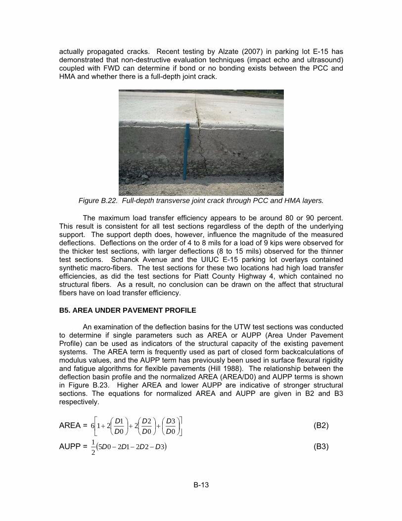
B-13

actually propagated cracks. Recent testing by Alzate (2007) in parking lot E-15 has demonstrated that non-destructive evaluation techniques (impact echo and ultrasound) coupled with FWD can determine if bond or no bonding exists between the PCC and HMA and whether there is a full-depth joint crack.

Figure B.22. Full-depth transverse joint crack through PCC and HMA layers.

The maximum load transfer efficiency appears to be around 80 or 90 percent.

This result is consistent for all test sections regardless of the depth of the underlying support. The support depth does, however, influence the magnitude of the measured deflections. Deflections on the order of 4 to 8 mils for a load of 9 kips were observed for the thicker test sections, with larger deflections (8 to 15 mils) observed for the thinner test sections. Schanck Avenue and the UIUC E-15 parking lot overlays contained synthetic macro-fibers. The test sections for these two locations had high load transfer efficiencies, as did the test sections for Piatt County Highway 4, which contained no structural fibers. As a result, no conclusion can be drawn on the affect that structural fibers have on load transfer efficiency.

B5. AREA UNDER PAVEMENT PROFILE

An examination of the deflection basins for the UTW test sections was conducted to determine if single parameters such as AREA or AUPP (Area Under Pavement Profile) can be used as indicators of the structural capacity of the existing pavement systems. The AREA term is frequently used as part of closed form backcalculations of modulus values, and the AUPP term has previously been used in surface flexural rigidity and fatigue algorithms for flexible pavements (Hill 1988). The relationship between the deflection basin profile and the normalized AREA (AREA/D0) and AUPP terms is shown in Figure B.23. Higher AREA and lower AUPP are indicative of stronger structural sections. The equations for normalized AREA and AUPP are given in B2 and B3 respectively.

AREA = ⎥⎦

⎤⎢⎣

⎡⎟⎠⎞

⎜⎝⎛+⎟

⎠⎞

⎜⎝⎛+⎟

⎠⎞

⎜⎝⎛+

03

022

01216

DD

DD

DD (B2)

AUPP = ( )322120521 DDDD −−− (B3)

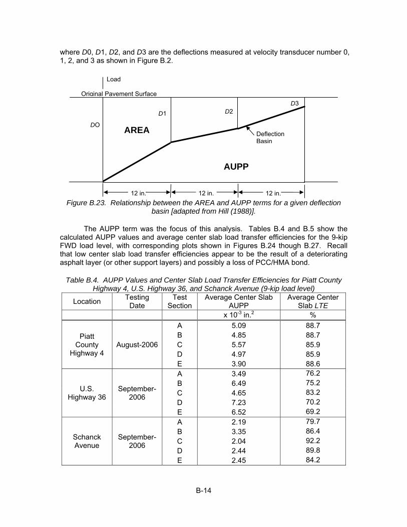
B-14

where D0, D1, D2, and D3 are the deflections measured at velocity transducer number 0, 1, 2, and 3 as shown in Figure B.2.

Figure B.23. Relationship between the AREA and AUPP terms for a given deflection

basin [adapted from Hill (1988)].

The AUPP term was the focus of this analysis. Tables B.4 and B.5 show the calculated AUPP values and average center slab load transfer efficiencies for the 9-kip FWD load level, with corresponding plots shown in Figures B.24 though B.27. Recall that low center slab load transfer efficiencies appear to be the result of a deteriorating asphalt layer (or other support layers) and possibly a loss of PCC/HMA bond.

Table B.4. AUPP Values and Center Slab Load Transfer Efficiencies for Piatt County Highway 4, U.S. Highway 36, and Schanck Avenue (9-kip load level)


Test Section

Average Center Slab AUPP

Average Center Slab LTE

x 10-3 in.2 %

Piatt County

Highway 4 August-2006

A 5.09 88.7 B 4.85 88.7 C 5.57 85.9 D 4.97 85.9 E 3.90 88.6

U.S. Highway 36

September-2006

A 3.49 76.2 B 6.49 75.2 C 4.65 83.2 D 7.23 70.2 E 6.52 69.2

Schanck Avenue

September-2006

A 2.19 79.7 B 3.35 86.4 C 2.04 92.2 D 2.44 89.8 E 2.45 84.2

DO

D2D3

D1

AREA Deflection Basin

AUPP

Original Pavement Surface

12 in. 12 in. 12 in.

Load

B-15

Table B.5. AUPP Values and Center Slab Load Transfer Efficiencies for UIUC E-15 Parking Lot (9-kip load level)


Parking Bay

Average Center Slab

AUPP

Average Center Slab

LTE x 10-3 in.2 %

UIUC E-15

Parking Lot

August-2006 1 7.83 90.0

September-2006 1 7.08 89.6 2 5.14 88.6 3 5.61 89.4

60.0

64.0

68.0

72.0

76.0

80.0

84.0

88.0

92.0

96.0

0.00 1.00 2.00 3.00 4.00 5.00 6.00 7.00 8.00 9.00 10.00

AUPP (x 10-3 in2)

Cen

ter S

lab

LTE

(%)

Section ASection BSection CSection DSection E

Figure B.24. Center Slab Load Transfer Efficiencies versus AUPP values for Piatt

County Highway 4 (9-kip load level).

60.0

64.0

68.0

72.0

76.0

80.0

84.0

88.0

92.0

96.0

0.00 1.00 2.00 3.00 4.00 5.00 6.00 7.00 8.00 9.00 10.00

AUPP (x 10-3 in2)

Cen

ter S

lab

LTE

(%)


Figure B.25. Center Slab Load Transfer Efficiencies versus AUPP values for U.S.

Highway 36 (9-kip load level).

B-16

60.0

64.0

68.0

72.0

76.0

80.0

84.0

88.0

92.0

96.0

0.00 1.00 2.00 3.00 4.00 5.00 6.00 7.00 8.00 9.00 10.00

AUPP (x 10-3 in2)

Cen

ter S

lab

LTE

(%)


Figure B.26. Center Slab Load Transfer Efficiencies versus AUPP values for Schanck

Avenue (9-kip load level).

60.0

64.0

68.0

72.0

76.0

80.0

84.0

88.0

92.0

96.0

0.00 1.00 2.00 3.00 4.00 5.00 6.00 7.00 8.00 9.00 10.00

AUPP (x 10-3 in2)

Cen

ter S

lab

LTE

(%)

Parking Bay 1 (August)Parking Bay 1 (October)Parking Bay 2 (October)Parking Bay 3 (October)

Figure B.27. Center Slab Load Transfer Efficiencies versus AUPP values for UIUC E-15

Parking Lot (9-kip load level).

These plots show a lack of correlation between AUPP values and load transfer efficiencies at the center of the UTW slabs, indicating that the magnitude of the AUPP value at a given location may not be able characterize the underlying support after placement of the UTW. However, it is hypothesized that the change in AUPP over time for a given section may be able to provide an indication of loss of bond or structural deterioration. As the PCC/HMA bond weakens, the support provided by the underlying layers is expected to decrease, resulting in higher AUPP values. It is recommended that FWD tests be conducted on distressed pavements prior to whitetopping and over regular time intervals once the overlay has been placed in order to provide the data necessary to examine the change in AUPP values over time as a means of characterizing the underlying support and the condition of the PCC/HMA bond.

B-17

B6. SUMMARY

FWD testing and analysis of the results indicate that high load transfer efficiencies mean the PCC overlay has good bond with the AC and strong support. High LTE could also indicate that joint cracking has not occurred but this would need to be visually confirmed or through other non-destructive evaluation techniques. Low load transfer efficiencies at the joint relative to the center of the slab LTE calculation means a full-depth joint crack has likely occurred. Low center slab load transfer efficiencies likely indicate a deteriorated support condition. Low load transfer efficiencies values may also indicate a loss of PCC/HMA bond. The maximum load transfer efficiency appears to be around 80 or 90 percent, regardless of the depth of the underlying support.

An examination was conducted to determine if deflection basin parameters can be used as indications of the structural capacity of the pavement systems. The results indicate that the magnitude of AUPP values may not be able to characterize the underlying support especially with the UTW layer present. However, the change in deflection profile parameters over time is suggested as a means of indicating the structural capacity of the underlying support and the condition of the PCC/HMA bond. The deflection basin parameter may be able to be used to indicate the structural condition of the existing distressed HMA layer prior to the concrete overlay but this must be further examined in the future.

C-1

APPENDIX C. CONCRETE MATERIAL TESTING

Evaluation of various concrete mixture designs used in ultra-thin whitetopping (UTW) pavement projects was undertaken to determine the influence of the material selection and proportioning on the performance of these pavements. The mixtures used in this study were found throughout Illinois as part of the Illinois Department of Transportation (IDOT) projects, projects found on the University of Illinois at Urbana-Champaign (UIUC) campus, a continuously reinforced concrete pavement used on the Dan Ryan expressway in Chicago, IL, or a project performed in Brazil. These projects were all evaluated for their fresh and hardened concrete properties, specifically investigating the fracture energy, composite concrete-asphalt section behavior, and shrinkage. Further information on test procedures and results are described in this appendix. C.1. MIX DESIGNS CHOSEN FROM EXISTING PROJECTS

A summary of the mixture designs chosen for the concrete material study are shown below in Table C.1 for the IDOT projects or in Table C.2 for other projects. The mixture proportioning, strength and distress levels are described in Appendix A.

Table C.1. Mixture Designs for the IDOT Projects

Location Schanck Avenue Int. of Vienna and Main Streets US Hwy 36 Cumberland County

Highway 2Piatt County Highway 4

District District 1, Mundelein District 9, Anna District 5, Tuscola District 5, Toledo District 5, MonticelloCoarse Agg 1972 1805 1704 1836 1957

Fine Agg 1001 1008 1035 1256 1220

Cement 515 755 755 575 534

Water 267 273 255 197 179

Fly Ash C 140 0 0 0 0

Strux Fibers 4 0 0 0 0AEA Daravair 1400 Daravair 1400 Daravair 1400 Daravair 1400 Daravair 1400Other admix WRDA 82 Daracem 65 Daracem 65 Daratard 17 Daracem 65

7 day Compressive Strength (psi) 3516 3553 - - -

14 day Flexural Strength (psi) - - 917 891 934

Time of Survey (yrs) - 3.3 5 0.7 3.6% Corner-Break Slabs - 14.63% 3.02% 0.00% 0.20%

%Transverse Cracks - 3.66% 1.04% 0.42% 0.30%

%Longitudinal Cracks - 3.14% 0.31% 0.00% 0.00%

% Debonded Slabs - 2.00% 2.04% 0.00% 0.00%

Distresses

Strengths

C-2

Table C.2. Other UTW Projects

Express Lanes Local Lanes SP-280 USP campus

lb/yd3 1894 1887 2013 1734type 022 CM 07 022 CM 11 Crushed Granite Crushed Granite

lb/yd3 1258 1230 831 1082type 029 FMM 20 027 FM 02 Round Quartz Round Quartz

Cement lb/yd3 435 435 742 802Water lb/yd3 230 230 298 340Silica Fume lb/yd3 0 0 74 48GGBF Slag lb/yd3 110 110 0 0

type Excel AEA (3523-01)

Daravair 1400 N/A none

fl.oz/yd3 N/A N/A 3 0

type Redi-set (767-01) WRDA 82 N/A N/A

fl.oz/yd3 N/A N/A 43 37type none none N/A N/A

fl.oz/yd3 0 0 140 62

w/cm wt ratio 0.42 0.42 0.37 0.40coarse/fine wt ratio 1.51 1.53 2.42 1.60% agg wt ratio 80.3% 80.1% 71.9% 70.3%

Fine Aggregate

Superplasticizer

Water Reducer

Air Entrainment

Dan RyanLocation

Coarse Aggregate

Brazil

C.2. CONCRETE FRACTURE TESTING

Fracture mechanics is a growing field of interest within pavement engineering. All of the research initiatives presented in this report utilized fracture mechanics theory and testing methods. Other concrete material properties (such as strength) were also measured for further evaluation of the material behavior. This appendix chapter summarizes the background behind using fracture mechanics in concrete pavement material characterization, explains the specific testing and analysis procedure used to determine fracture properties of the concrete mixtures, and presents and discusses the measured concrete fracture properties.

C.2.1. Background

The current design of rigid pavements relies on hardened concrete properties such as compressive, tensile and flexural strengths. Although these properties have been used successfully for years, the existing design inputs do not capture the entire cracking behavior of the pavement structure. By quantifying additional failure properties of the concrete, a better grasp of how the concrete pavement performs throughout its life can be ascertained. Through fracture mechanics, material parameters indicating the initiation and growth of cracks and the nominal load capacity of initial cracked structures can be derived. The fracture toughness has been used to describe the rate of crack propagation through the concrete. The use of fracture energy with a cohesive zone model can quantify the load capacity of a beam or slab (Park et al. 2007) or indicate the ability of a concrete material to transfer load across a crack or joint (Chupanit and Roesler, 2005).

Concrete is often considered a brittle material, which alludes to the possibility of analyzing it with linear elastic fracture mechanics. In reality, concrete is a quasi-brittle material which exhibits a significant amount of nonlinear behavior especially after the

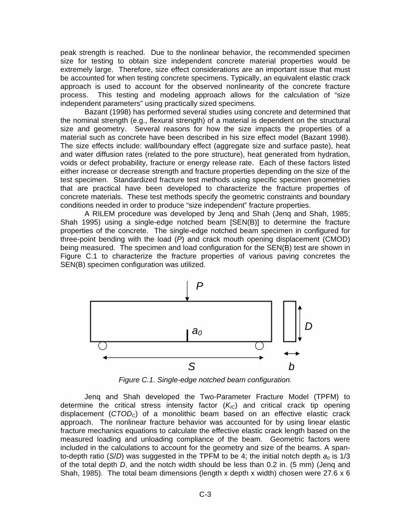
C-3

peak strength is reached. Due to the nonlinear behavior, the recommended specimen size for testing to obtain size independent concrete material properties would be extremely large. Therefore, size effect considerations are an important issue that must be accounted for when testing concrete specimens. Typically, an equivalent elastic crack approach is used to account for the observed nonlinearity of the concrete fracture process. This testing and modeling approach allows for the calculation of “size independent parameters” using practically sized specimens.

Bazant (1998) has performed several studies using concrete and determined that the nominal strength (e.g., flexural strength) of a material is dependent on the structural size and geometry. Several reasons for how the size impacts the properties of a material such as concrete have been described in his size effect model (Bazant 1998). The size effects include: wall/boundary effect (aggregate size and surface paste), heat and water diffusion rates (related to the pore structure), heat generated from hydration, voids or defect probability, fracture or energy release rate. Each of these factors listed either increase or decrease strength and fracture properties depending on the size of the test specimen. Standardized fracture test methods using specific specimen geometries that are practical have been developed to characterize the fracture properties of concrete materials. These test methods specify the geometric constraints and boundary conditions needed in order to produce “size independent” fracture properties.

A RILEM procedure was developed by Jenq and Shah (Jenq and Shah, 1985; Shah 1995) using a single-edge notched beam [SEN(B)] to determine the fracture properties of the concrete. The single-edge notched beam specimen in configured for three-point bending with the load (P) and crack mouth opening displacement (CMOD) being measured. The specimen and load configuration for the SEN(B) test are shown in Figure C.1 to characterize the fracture properties of various paving concretes the SEN(B) specimen configuration was utilized.

Figure C.1. Single-edge notched beam configuration.

Jenq and Shah developed the Two-Parameter Fracture Model (TPFM) to

determine the critical stress intensity factor (KIC) and critical crack tip opening displacement (CTODC) of a monolithic beam based on an effective elastic crack approach. The nonlinear fracture behavior was accounted for by using linear elastic fracture mechanics equations to calculate the effective elastic crack length based on the measured loading and unloading compliance of the beam. Geometric factors were included in the calculations to account for the geometry and size of the beams. A span-to-depth ratio (S/D) was suggested in the TPFM to be 4; the initial notch depth a0 is 1/3 of the total depth D, and the notch width should be less than 0.2 in. (5 mm) (Jenq and Shah, 1985). The total beam dimensions (length x depth x width) chosen were 27.6 x 6

b

a0D

P

S

C-4

x 3.1 in. (700 x 150 x 80 mm) with a span of 23.6 in. (600 mm) and an initial notch depth of 2 in. (50 mm). It was recommended that four replicates of each beam be tested (Karihaloo and Nallathambi, 1991).

C.2.2. Fracture Testing Procedure

The Two-Parameter Fracture Model beams were cast in steel molds and a notch was saw cut 24 hours before testing using a block saw with a diamond blade. Prior to testing two aluminum knife edges were placed 0.5 in. (10 mm) apart with a quick-set epoxy. An INSTRON clip gauge measuring opening displacement up to 0.18 in. (4 mm) range was clipped onto the knife edges to measure the crack mouth opening displacement (CMOD). An 11-kip (50-kN) MTS machine applied the monotonic load to the specimens. Cyclic compliance testing was useful for describing the deformation and crack propagation in a material. A LABVIEW program was developed to remotely control the testing of the concrete specimen through the clip gauge readings.

During testing a seating load of 0.011 kips (0.05 kN) was placed on each specimen followed by a constant opening displacement rate of 0.0254 in./sec (0.001 mm/sec). After the load decreased to 95 percent of the peak load, the data acquisition program automatically unloads the specimen over a 10 second period. The specimen was then again re-loaded and unloaded at 95 percent of the second peak load. The program was designed to continue this process for n-cycles. A plot of loading and unloading cycles is shown in Figure C.2. For the majority of the experiments tested in this research, on the 3rd cycle, the opening displacement rate was increased to 0.0012 in./sec (0.005 mm/sec) and the program manually adjusted to not unload (i.e. continue constant displacement control) until the clip gauge went out of range or the load reached zero, whichever was first.

Figure C.2. Loading and Unloading Cycles for SEN(B) concrete specimen.

C.2.2.1. Run-out test for FRC

For some of the concrete materials, such as fiber-reinforced concrete (FRC), the clip gauge generally went out of range before the failure of the beam. Therefore a yo-yo gauge (a string extender linear transducer) with a 2 in. (50 mm) range was attached to

0

0.5

1

1.5

2

2.5

3

3.5

4

0 0.2 0.4 0.6 0.8 1

CMOD (mm)

Load

(kN)

C-5

one side of the beam with epoxy before the test (see Figure C.3 for a photograph of the yo-yo gauge and clip gauge on the beam). The testing procedure for the FRC beams was still the same for the two initial cycles. A desktop computer controlled the test for the first two cycles. After the first two cycles were completed, the control of the test was switched over to a user-defined position ramping speed of 0.12 in./min (1 mm/min) vertical machine position control using the 8800 Instron controls until failure was reached [determined manually when the load fell below 0.011 kips (0.05 kN)]. An additional laptop computer was used for data recording of all cycles and the run-out beyond the range of the clip gauge. Figure C.4 shows the 8800 Instron control machines and computers used.

Yo-yo gauge

Clip gauge

Loading pin

NotchYo-yo gauge

Clip gauge

Loading pin

Notch

Figure C.3. Photograph of the single-edge notched beam during testing.

(a) (b) (c)

Figure C.4. Testing equipment for fracture testing: (a) Instron control tower, (b) Instron panels, and (c) data acquisition computers.

C-6

C.2.3. Data Calculation Analysis

In order to plot the load-CMOD curve for each specimen, the clip gauge and yo-yo gauge data were correlated to each other and the change (based on the initial gauge reading) in corrected displacement is the CMOD. Figure C.5 shows a schematic of the first and second loading cycles of the SEN(B).

Pc

CMODcP CMODc

e

Ci

P

CMOD

Cu

Pc

CMODcP CMODc

e

Ci

P

CMOD

Cu

Figure C.5. Schematic of loading and unloading cycles of a SEN(B) specimen used to

compute initial compliance Ci and unloading compliance Cu. C.2.3.1. Analysis Inputs

The initial fracture properties were calculated from the loading and unloading compliance, the peak load (Pc), the beam weight, and the initial notch depth. The beam weight was determined by multiplying the beam volume by the fresh concrete unit weight of the mixture measured during casting. The initial notch depth sometimes varied within a specimen due to the rate at which the beams were cut under the saw; a0 was measured from the bottom surface of the beam to the top of the rounded notch tip.

The loading compliance (Ci) was calculated as the inverse of the slope from 10 percent of the peak load until 50 percent of the peak load. This was estimated to be the linear elastic range and ignored any initial seating load discontinuities in the curve. The unloading compliance (Cu) was the inverse of slope of the unloading curve. It was estimated that Cu should be calculated between 10 percent of the peak load and 80 percent of the peak load on the unloading curve. Since the calculation of Cu was dependent on the points chosen on the unloading curve other methods to determine of Cu were investigated and presented below.

C-7

C.2.3.1. Compliance Determination

The definition of loading and unloading compliance is shown in Figure C.5. The compliances could be difficult to determine from the load versus CMOD curves since it involved some user subjectivity to determine the elastic part of the unloading compliance. The initial loading compliance for an elastic material was assumed to be roughly the inverse of the material loading stiffness. However, different methods exist for determining the initial slope such as tangent, secant, or chord stiffness. Computing the unloading compliance was even more difficult due to the inherent nonlinear elastic and inelastic response of the material during unloading. Ideally the test should be set up to unload immediately after the peak load was reached for the determination of the unloading compliance. Due to uncertainty in when the peak load level has been reached, the RILEM method proposed by Jenq and Shah (1985) suggested unloading the specimen at 95 percent of the peak load with the assumption that the unloading slope at this load level was assumed to be similar to that from the actual peak load. This unloading technique also assumed there is no additional crack propagation from the peak load to the 95 percent peak value, which can lead to an error in the critical crack length calculation.

In order to eliminate operator controlled error, Jansen et al. (2000) performed a study that implemented a focal point method for computing the unloading compliance. By extrapolating slopes (determined from the unloading curve) from several load/unload cycles back to a focal point; the need to unload a beam at 95 percent of the peak load was no longer required. A diagram of this process can be seen in Figure C.6. In the paper by Jansen et al. (2000), little information was provided on how the actual compliance values for each unloading cycles were determined (tangent, chord, or secant compliance).

Figure C.6. Focal point method for compliance determination [from Jansen et al. (2000)].

C-8

Computing the critical crack length could be determined by drawing a line between the focal point and the peak load and then calculating the unloading compliance. The critical crack length determined using the peak load compliance was always smaller than a compliance taken at any load after the peak load had been reached (when the crack has propagated beyond the critical length). Smaller critical crack lengths led to smaller critical stress intensity factor, critical crack tip opening displacement, and initial fracture energy values. In other words, Jansen et al. (2000) found that the KIC and CTODC values determined with the focal point method were consistently reduced by 12 and 38 percent, respectively, compared to just computing the unloading compliance from 10 and 80 percent of the peak load.

A specific feature that was noticed between specimens was that the duration or displacement at which the 95 percent post-peak unloading load was highly variable. Some specimens demonstrated a long gradual softening curve initially after the peak and the 95 percent load was not reached until a larger CMOD value; other specimens demonstrated almost instantaneous load reduction after the peak and thus the unloading began much sooner at smaller CMOD values. Either a manual unloading response or the focal point method may be desired in order to reduce the variability from those specimens exhibiting the more gradual post-peak curve.

The variability of the calculated KIC and CTODC values using the focal point method was determined to be similar to the traditional TPFM, according to Jansen et al. (2000). For example, the coefficient of variation on KIC with the focal point method was 6.5 percent and was 5.1 percent for the TPFM; similarly, the coefficient of variation on CTODC was 37 percent using the focal point method and 21 percent using the TPFM. The focal point method was developed to supplement the TPFM to allow users to unload at any load level and still compute the relevant initial fracture properties. The focal point method may provide a more accurate result on fracture parameters however based on the larger variation reported in Jansen et al. (2000), it may not be as precise. For the studies performed in this report, the TPFM with unloading from 95 percent of the peak load was used because the computer running the test was able to precisely detect the load level for automatic unloading at this level of loading. Due to the lack of improved accuracy for the focal point method, the loading and unloading compliances were respectively found by manually selecting specific data points along the loading (at 10 and 50 percent of the peak load) and unloading (at 80 and 10 percent of the peak load) curve as stated in the previous section.

C.2.3.1. Calculation of Initial Fracture Properties

The two fracture parameters determined through the TPFM were the critical stress intensity factor (KIC) and the critical crack tip opening displacement (CTODC) (Jenq and Shah, 1985; Shah 1995). These were computed by first obtaining the critical effective crack length (ac). By equating, the concrete’s modulus of elasticity from the loading and unloading curves (E = Ei = Eu) as shown in equations C1a and C1b, the critical effective crack length could be determine as follows:

bDCgSaE

ii 2

020 )(6 α= (C1a)

bDCgSaE

u

ccu 2

2 )(6 α= (C1b)

where (S) was the span, (D) the depth, (b) the width, (a0) the initial notch depth of the beam α0 the initial notch/depth ratio, αc the critical notch/depth ratio and g2(α) the opening displacement geometric factor for the SEN(B) specimen given by equation C2.

C-9

232

2 )1(66.004.287.328.276.0)(α

αααα−

+−+−=g (C2)

Once the ac was computed, then the critical stress intensity factor (KIC) could be

calculated from the following (equation C3),

bDDagaS

LSWPcK ccIC 2

10 2

)/()/5.0(3

π+= (C3)

where (Pc) was the peak load, W0 was the weight of the specimen, L was the length of the specimen and (g1) was the stress intensity factor geometric function for the beam specimen defined as follows (equation C4).

[ ]2/3

2

1)]/(1)][/(21[

)/(70.2)/(93.315.2)/1)(/(99.1)(

DaDaDaDaDaDa

Da

gcc

ccccc

−+

+−−−=

π (C4)

Finally, the CTODC could be computed using equation C5.

2/12

002

22

0

])/()/[(*)](149.1081.1[))/(1(

*)/(

*)/5.0(6

⎥⎦

⎤⎢⎣

⎡ −−+−

+=

aaaaDa

aa

bEDDagSa

LSWPCTOD

ccc

oc

cccc

(C5)

By using a thin SEN(B), plane stress was assumed and the critical energy

release rate (Gf), or also known as the initial fracture energy, was related to KIC and the modulus of elasticity, E, by equation C6.

EK

G ICf

2

= (C6)

C.2.3.1. Total Fracture Energy

The testing data from the SEN(B) concrete specimen could also be used to calculate the area under the load-CMOD curve which can be related to the concrete total fracture energy (GF). Monotonic loading until specimen failure was usually employed instead of a cyclical load-unload testing process for determining the total fracture energy. Therefore the static cycles of the tested data were manually removed such that an envelope curve was drawn using the following: the initial loading data till the peak load, the data from the peak load to 95 percent of the peak load on each cycle, the remaining curve after cycles were complete until failure (at 0.05 kN).

According to Hillerborg (1985), the total fracture energy (GF) or work of fracture was determined as the total energy (Wt), normalized to the fracture area baD )( 0− . The total energy (Wt) was calculated using the sum of the area under the load (P) vs. CMOD envelope curve (Wr), and Pwδf, where Pw was the equivalent self weight force, and δf was the CMOD displacement corresponding to the applied load (zero) at failure. The equivalent self weight force and total fracture energy were calculated using equations C7 and C8, respectively.

LSW

Pw 20= (C7)

baDPW

baDW

G fwrtF )(

2)( 00 −

+=

−=

δ (C8)

C-10

The total fracture energy has more variability, especially compared to the initial fracture energy. Bazant et al. (2002) described that much of the scatter in GF calculation comes from: 1) inherent randomness in the tail end of the load-CMOD curve, 2) uncertainty in extrapolating the tail end of the curve to zero load, and 3) difficulty eliminating non-fracture sources of energy dissipation.

There is little information in the research literature as to the exact cut off criterion for the total fracture energy computation as it pertains to fiber-reinforced concrete (FRC) materials. The Hillerborg method was created for computing the fracture energy of plain concrete specimens that undergo complete specimen failure. With plain concrete, the area under the load-displacement curve from 0.05 kN to 0.0 kN load at failure is almost negligible. However, for such materials, like FRC, which have long post-peak curves and large displacements, the area under the load-displacement curve depended highly on the load to cut-off the area calculation. If the point of complete failure was determined to be at the same load as the initial seating load, the fracture energy would be drastically lower for some FRC mixtures than if the point of failure were determined when the load reached a zero value with the testing apparatus. See Figure C.7 for a schematic example of the area differences for FRC mixtures. For the FRC mixtures used in this report, the GF was consistently computed as the area under the load-CMOD curve till 0.05 kN load (which was the applied load corresponding to the seating load). The Hillerborg method may still be a valid for determining the fracture energy. Clarification should be made for future testing to determine whether a load of zero or the initial seating load should be used as the cut-off criterion for the total fracture energy.

0

0.5

1

1.5

2

2.5

3

3.5

4

4.5

5

0 10 20 30 40 50

CMOD (mm)

Load

(kN

)

G F = area under Load verses CMOD Fracture area

up to Load P = 0.05 kN

up to Load P = 0 kN

Figure C.7. GF calculation for a straight synthetic FRC specimen.

C-11

C.2.3.1. Summary

All of the fracture testing for projects presented in this report utilized the SEN(B) specimens for determining fracture properties. The fracture properties were all calculated using the same equations as described earlier. These fracture properties were used to evaluate the effectiveness of different concrete materials for their post-peak performance.

C.3. FRACTURE PROPERTIES OF PAVING MIXTURES

Laboratory research has been performed for this report to understand how age of testing, concrete material proportioning and constituent selection affect the concrete fracture properties. Concrete mixtures presented in this section originated from other existing pavement projects (see Appendix A). The predictions of concrete fracture properties made by other researchers were also evaluated with the measured data presented herein. C.3.1. Background C.3.1.1. Past Studies

Several researchers have attempted to predict fracture properties with respect to age or material properties. Mindess et al. (2003) have reported that the fracture energy did not vary with age, compressive strength, or w/cm ratio but instead depended on the strength of the coarse aggregate. Bazant and Becq-Giraudon (2002) performed a statistical study of fracture properties. They used a database of fracture and strength properties for different specimen types and mixture designs reported in the literature. An equation was developed based on the compressive strength of the concrete f’c, the maximum coarse aggregate size da, and the water-cement ratio, to compute the initial fracture energy Gf and total fracture energy GF. Similar equations developed by other researchers were also reported in the Bazant and Becq-Giraudon paper, but are not included here. Bazant and Becq-Giraudon described an equation to compute the fracture energy of concrete, shown here as equations C9a and C9b. They reported coefficients of variation of 18 and 30 percent for the initial fracture energy and total fracture energy, respectively.

30.022.046.0

)/(27.11

1051.0'

44.1 −⎟⎟⎠

⎞⎜⎜⎝

⎛+⎟⎟

⎠

⎞⎜⎜⎝

⎛= cmw

dfG ac

f (C9a)

GF = 2.5 Gf (C9b)

Zollinger et al. (1993) conducted age effect testing (at 1, 7, and 28 days) with

Texas concrete paving mixtures containing various coarse aggregate sources of crushed limestone or river gravel. The study concluded that the critical stress intensity factor KIC and the fracture process zone size increased with the age for each concrete mixture. The brittleness of the concrete (computed as the specimen depth divided by the critical effective crack length) was also determined to be greatest at the early ages (before 28 days). For concrete specimens containing river gravel, the critical stress intensity factor was plotted against age, normalized to 28 days, and shown in Figure C.8. An empirical formula shown in equation C10 was developed by Zollinger et al. to predict the critical stress intensity factor at different ages (t in days) based on a 28-day test (KIC

28).

C-12

4/1

28 28⎟⎠⎞

⎜⎝⎛=

tKK

IC

IC (C10)

C.3.1.1. Motivation

The results in this section used the concrete mixture designs primarily from the UTW field mixtures (see Table C.1) to evaluate the specific influences of age, aggregate type, and cement content on the measured fracture properties. In addition, the equations proposed by Bazant and Becq-Giraudon and by Zollinger et al. to determine fracture properties will also be evaluated. A standardized age for testing fracture properties was also determined in this section for paving mixtures used in Illinois.

Figure C.8. Stress intensity factor versus age both normalized at 28 days [from Zollinger

et al. 1993]. C.3.2. Age Effect Studies

It is well known that conventional concrete hardened properties such as strength and elastic modulus increase with age. The material properties of a pavement will vary with time as the concrete continues to hydrate and as climate and traffic loading alters the stresses or strains within the concrete. The strength gain and hydration of concrete are greatly impacted by factors such as temperature, moisture or relative humidity, geometry of the specimen, and microstructure of the concrete. An age effect study was undertaken to verify the evolution of concrete paving mixtures fracture properties for a variety of material constituents and proportions. In addition, it was necessary to analyze concrete paving mixtures with age independent fracture properties. Therefore a standard age should be determined for further fracture testing of concrete mixtures.

C-13

The current study included a wide a variety of mixtures, shown in Table C.1, using low and high cement contents, a fiber-reinforced concrete mixture, and mixtures containing slag, fly ash, or silica fume. The age effect fracture testing analyzed specimens cured from 7 to 90 days. The Anna and Low Cement mixtures were derived from IDOT ultra-thin whitetopping (UTW) field projects for the intersection project at Vienna and Main Streets in District 9 and the Piatt County Highway 4 project in District 5 (field mixtures shown in Table C.1), respectively. The Parking Lot mixture was sampled directly from a field project on the University of Illinois at Urbana-Champaign parking lot E-15. No air entraining agent was added to the Parking Lot mixture in the field according to the ready-mix supplier. The Brazil 1 Mixture is based on SP-280 highway mixture proportions (shown in Table C.2) with an adjustment in the coarse-to-fine aggregate blending and without any water-reducing admixture. The mixture proportions shown in Table C.3 have all been normalized to one cubic yard batches of concrete.

The same coarse aggregate type and maximum size of 1 in. (25 mm) was used for all mixtures in this age effect study. Other researchers found the coarse aggregate type and maximum size to control the post-peak fracture behavior (Bazant and Becq-Giraudon, 2005; Mindess et al. 2003; Zollinger et al. 1993); a small research study is described later in this appendix to compare coarse aggregate effects.

Table C.3. Age Effect Concrete Mixture Designs

Anna Low Cement Parking Lot Dan Ryan Brazil 1

Cement lb/yd3 774 561 434 447 735Fly Ash lb/yd3 0 0 135 0 0Slag lb/yd3 0 0 0 113 0Silica Fume lb/yd3 0 0 0 0 73Water lb/yd3 280 246 222 236 295Coarse Aggregate lb/yd3 1851 1924 1929 1939 1761Fine Aggregate lb/yd3 1034 1282 1231 1264 1084Fibers lb/yd3 0 0 3 0 0Air Entrainer ml/yd3 114 83 0 66 271Water-Reducer ml/yd3 172 498 770 397 0Super Plasticizer ml/yd3 0 0 0 0 2391

0.36 0.44 0.39 0.42 0.37w/cm ratio

All mixtures for the age effect study were tested with the SEN(B), compressive strength, split-tensile strength, and elastic modulus at 7, 28 and 90 days with the exception of the Parking Lot mixture, which came directly from the field and properties were only measured at 7 and 28 days. All mixtures were tested in with the standard beam flexural specimen (ASTM C 78) at the following ages: Low Cement, Dan Ryan and Brazil 1 mixtures at 28 days; Anna County mixture at 14 days; Parking Lot mixture at 7 days. The Anna mixture was tested as part of the composite beam studies (see section C.4) and therefore also was tested at 14 days for fracture properties. Two specimen replicates were tested for each hardened property realizing that this would increase the

C-14

variability in the results but it was important to cast all specimens for one age in one batch.

C.3.2.1. Age Effect Results

The hardened property testing plan of for each mixture and batch at the various ages (7, 28 or 90 days) is shown in

Table C.4. The fresh concrete properties for each concrete batch are presented

in Table C.4. Each batch of the same mixture proportions produced similar fresh

concrete properties which meant that these batches should produce similar hardened properties.

C.3.2.1. Load versus CMOD curves

The loads versus CMOD curves for the SEN(B) specimens of each mixture in the age effect study are shown in Figures C.9 through C.11 at 7, 28 and 90 days, respectively. The Brazil 1 mixture contained a high amount of entrained air which caused the consistently low peak load compared to other mixtures. The post-peak behaviors of all curves, with the exception of the FRC (Parking Lot) mixture, were similar.

Table C.4. Age Effect Batch Testing Plan and Fresh Properties

Parking Lot

batch 1 2 1 2 1 1 2 1 27 28, 90 7, 90 28 7, 28 7, 90 28 7, 90 287 28, 90 7, 90 28 7, 28 7, 90 28 7, 90 287 28, 90 7, 90 28 7, 28 7, 90 28 7, 90 28- 28, 90 7, 90 28 7, 28 7, 90 28 7, 90 287 28 - 28 - - 28 - 28

2.75 2.50 5.25 5.00 - 1.00 1.50 9.50 9.75148 147 144 144 - 148 150 129 1363.8 3.7 6.0 6.3 - 3.7 2.8 13.3 10.3

Unit Weight Air Content

Anna

Fresh Properties of BatchMOR

Slump (in.)

SEN(B)CompressionSplit-TensionElastic

Low Cement Dan Ryan Brazil 1

Age(s) tested

C-15

0

0.5

1

1.5

2

2.5

3

3.5

4

4.5

0 0.2 0.4 0.6 0.8 1CMOD (mm)

Load

(kN

)AnnaLow CementParking LotDan RyanBrazil 17 days

Figure C.9. Load versus CMOD curves for SEN(B) specimen at 7 days.

0

0.5

1

1.5

2

2.5

3

3.5

4

4.5

0 0.2 0.4 0.6 0.8 1CMOD (mm)

Load

(kN

)

AnnaLow CementParking LotDan RyanBrazil 128 days

Figure C.10. Load versus CMOD curves for the SEN(B) specimen at 28 days.

C-16

0

0.5

1

1.5

2

2.5

3

3.5

4

4.5

5

0 0.1 0.2 0.3 0.4 0.5 0.6 0.7 0.8 0.9 1

CMOD (mm)

Load

(kN

)Anna Low CementDan RyanBrazil 190 days

Figure C.11. Load versus CMOD curves for the SEN(B) specimen at 90 days.

The CMOD value at the specimen peak load decreased with age from about 0.04

in. (1 mm) to 0.024 in. (0.6 mm) seen in Figures C.9 and C.11, respectively. This behavior corresponded to an increase in peak strength and toughness of the specimens and an opening width reduction with age. The reason the CMOD at failure decreased with age was the interfacial transition zone became stronger with time and therefore the concrete began fracturing through the bulk matrix and aggregates. Specimens at 90-days all showed a flat fracture plane through the aggregate and bulk matrix, while 7-day specimens showed a tortuous fracture path around the aggregates.

C.3.2.1. Measured Properties

A summary of the strengths and fracture properties (averaged from two specimens) of the age effect study can be seen in Table C.5. The coefficient of variation (COV) is also presented in Table C.5 for each measured property. Overall the fracture and strength properties increased with specimen age as expected. A comparison between compressive strength to split-tensile strength, peak load and initial fracture energy is shown in Figure C.12. There were a few discrepancies in strength gain such as Brazil 1 specimens had a higher average compressive strength at 28 days and the Low Cement specimens had a higher average split-tensile strength at 28 days. For both of these cases, the 28-day specimens were cast in a separate batch than the 7- or 90-day specimens which could be impacted by the altered air contents or consolidation differences used to cast the specimens from each batch. The Brazil 1 mixture had very high air contents and there was 3 percent less air in the 28-day specimens which likely led to the increased compressive strength.

C-17

Table C.5. Age Effect Strength and Fracture Properties

COV COV COV COV COV7 5.60 0% 4.17 6% 3.65 12% 4.41 6% 3.65 9%

28 6.46 10% 4.90 5% 5.22 3% 6.17 4% 5.93 0%90 7.28 5% 5.90 3% - - 7.16 5% 5.26 1%

7 513 33% 360 9% 436 17% 520 0% 338 24%28 549 15% 536 14% 573 5% 524 3% 508 14%90 662 4% 512 10% - - 640 8% 541 11%

7 3.46 17% 3.51 14% 2.98 5% 3.27 22% 2.26 0%28 3.69 10% 2.98 3% 3.94 10% 4.00 9% 3.04 2%90 4.20 1% 3.95 5% - - 28.23 * 2.63 8%

7 0.023 16% 0.017 30% 0.010 11% 0.016 30% 0.019 16%28 0.016 13% 0.018 41% 0.015 21% 0.029 13% 0.013 1%90 0.024 40% 0.022 7% - - 0.025 * 0.023 13%

7 1.07 16% 0.966 15% 0.74 5% 0.93 7% 0.67 8%28 1.05 1% 0.910 16% 1.14 0% 1.37 1% 0.79 1%90 1.32 14% 1.21 2% - - 1.42 * 0.78 7%

7 50 32% 43 40% 22 3% 35 10% 28 8%28 40 7% 34 22% 47 2% 68 2% 32 4%90 60 32% 54 14% - - 72 * 40 11%

7 83 22% 127 23% 164 19% 99 14% 83 6%28 115 2% 89 13% 1,140 20% 135 5% 102 11%90 102 20% 131 12% - - 141 * 92 20%

* one beam was omitted due to testing errors.

G F (N/m)

Dan Ryan Brazil 1

CTOD C

(mm)

Anna Low Cement Parking LotAge (day)

P c (kN)

K IC

(MPa m1/2)

G f (N/m)

Compressive Strength (ksi)

Split-Tensile Strength (psi)

C.3.2.1. Initial Fracture Properties

In general, the peak loads obtained in the fracture testing show a similar trend with age as the compressive strengths, see Figure C.12b. Based on the data in Table C.5, little difference could be seen in the magnitude of initial fracture property results (Gf, KIC, CTODC) between mixtures at any age. On average for all the mixtures, 75 percent of the fracture and strength properties were realized by 7 days and 85 percent by 28 days. The initial fracture energy of the Parking Lot mixture (containing fiber reinforcement) doubled between 7 and 28 days.

C-18

300350400450500550600650700

3,000 5,000 7,000 9,000

f'c (psi)

f't (p

si)

2

2.5

3

3.5

4

4.5

5

3,000 5,000 7,000 9,000

f'c (psi)

P c (k

N) 7 days

28 days90 days

(a) (b)

0

10

20

30

40

50

60

70

80

3,000 5,000 7,000 9,000

f'c (psi)

Gf

(N/m

)

7 days28 days90 days

(c)

Figure C.12. (a) Split-tensile strength and (b) SEN(B) specimen peak loads and (c) initial fracture energies compared to compressive strength.

C.3.2.1. Total Fracture Energy

For the non-reinforced (plain) concrete mixtures, the total fracture energy did increase with age and ranged in values between 83 N/m to 141 N/m. The total fracture energy of the FRC mixture (Parking Lot) increased by almost seven times between 7 and 28 days. The FRC mixture used in the Parking Lot was significantly higher in total fracture energy than other non-reinforced concrete mixtures at 28 days. Slight variation in crack propagation seen in the load-CMOD curves may produce the variation in total fracture energy seen in Table C.5; again porosity caused from air voids or large aggregates found in the fracture plane may also contribute to variation in the total fracture energy.

C.3.2.1. Stress Intensity Factor

For the mixtures studied in this report, a plot to compare stress intensity factor versus age is shown in Figure C.13. The study previously mentioned by Zollinger et al. (1993), proposed that equation 10 be used to determine the critical stress intensity factor

C-19

at different ages. This trend line (raised to the 0.25 power) fit the river gravel data from the Zollinger et al. study shown in Figure C.8, but does not match all the mixtures tested in this age effect study for the age range of 7 to 90 days. The change in properties after 7 days is much less than Zollinger’s model would predict. A shallow trend was plotted against the Zollinger et al. trend line in Figure C.13 to more accurately match some of the data here; the shallow trend line proposed altered equation 10 such that the ratio of (t/28) was raised to a value between 0.05 rather than 0.25. It should be noted that Zollinger’s equation was originally based on fracture toughness data at 1, 7, 14, 21, and 28 days, which was different than the time horizon used in this testing program.

0.0

1.0

2.0

0 20 40 60 80 100

Age (days)

K IC

/ K

IC28

AnnaLow CementParking LotDan RyanBrazil 1(t/28)^0.25(t/28)^0.05

Figure C.13. Stress intensity factor verses age for various mixtures.

C.3.2.1. Sample Preparation and Variability

Specimens from different batches often demonstrated different fracture properties. For example, the 7-day Anna specimens showed higher initial fracture property results than the 28- or 90-day specimens. Opposite of the strength gain seen in the Low Cement specimens, the 28-day fracture properties such as Gf, KIC, and GF decreased from the 7-day results (possibly driven by the increased air voids or some casting issue). The Brazil 1 mixture 28-day specimens also showed higher KIC, and GF values than at 90 days.

Bazant and Becq-Giraudon (2002) determined in a statistical study that the COV for initial and total fracture energy were on the order of 18 and 30 percent, respectively. Table C.5 supports previous researcher findings that fracture properties have large COV (Bazant and Becq-Giraudon, 2002; Bazant et al. 2002). In fact, the CTODC values had the greatest average COV, followed by Gf and GF. The 7-day fracture test results demonstrated high coefficients of variability (see Table C.5) for the material properties desired, compared to the 28- and 90-day testing. These results support other research literature findings that fracture properties can have larger coefficients of variability, especially at early ages.

C-20

C.3.2.1. Summary

One of the main goals of the age testing with the SEN(B) specimens was to determine the optimum age for fracture testing of concrete materials. Like strength testing, fracture properties increase with age, and therefore some change in properties with time was expected. It was determined that an age such as 28 days would be more appropriate to use as a reference time since the coefficient of variability after this point in time was relatively lower and little change occurred between 28 and 90 days.

C.3.3. Mixture Proportioning Effects

The choice in material proportioning can affect some of these properties; for example, higher cement contents tend to increase shrinkage within the concrete, although it may also aid in increasing the compressive and tensile strength and initial fracture energy of the concrete as well. Material type selection can also be important, for example, coarse aggregate type, proportion, and maximum size will have an effect on the hardened concrete properties and can even have a larger impact on the fracture behavior of the concrete pavement.

In this research, no specific mixture proportioning factorial was designed to examine the optimum mixture design proportions for maximum fracture properties for rigid paving mixtures. However, the various mixtures used in this research were chosen based on their diversity in mixture constituents and/or proportioning and the fact that they had been used for some type of rigid pavement project in the field. For example, the Anna mixture was selected to compare fracture properties with higher cement contents relative to lower cement contents (see Table C.1 for Anna and Low Cement mixture proportions). The Brazil 1 mixture contained silica fume and it was derived from the SP-280 highway project (Sao Paulo, Brazil), which required high early strength concrete. The Dan Ryan mixture provided an alternative comparison with its use of slag to replace a percentage of cement with a similar total cementitious content as the Low Cement mixture. The Parking Lot mixture incorporated fly ash as a supplementary cementitious material and included fiber-reinforcement. The following sub-sections describe the mixture proportioning effects.

C.3.3.1. Cement content

There should be enough cement to cover all of the aggregates or fibers in the mixture and to meet the design and opening strength. However, the high cost of cement and the hydration products potential to shrink upon drying typically results in specifications to minimize the amount of cement in the mixture. Cementitious contents for these studies ranged from approximately 560 to 570 lb/yd3 for the Dan Ryan, Low Cement and Parking Lot mixtures up to 774 lb/yd3 and 808 lb/yd3 for the Anna and Brazil 1 mixtures, respectively.

Based on the results presented in Table C.5, the Anna mixture showed higher strengths and initial fracture properties than most of the lower cementitious content mixtures (Low Cement, Dan Ryan, and Parking Lot mixtures) especially at the 7 day age. A plot of the compressive strength and initial fracture energy versus cement content shown in Figure C.14 emphasizes that no correlation was found between these properties. The total fracture energy was also unaffected by the cement content. The impact of cement content and shrinkage is explained later in section C.4.6. The affect of

C-21

the supplementary cementitious materials was not specifically studied, thus no conclusion on their impact on fracture properties can be drawn here.

0

10

20

30

40

50

60

200 300 400 500 600 700 800 900

Cement Content (lb/yd3)

f' c (M

Pa)

0

10

20

30

40

50

60

70

80

Gf (

N/m

)

Compressive StrengthInitial Fracture Energy

Figure C.14. Compressive strength and initial fracture energy versus cement content.

C.3.3.1. Coarse-Fine Aggregate Ratio

The coarse and fine aggregates could be volumetrically optimized for maximum packing density. Ideally, the maximum packing density was the most economically viable to obtain the minimum volume of required cementitious material to fill voids (cement was the most expensive component). This optimized packing density was impacted by the gradation curves and aggregate surface texture (Mindess et al. 2003). For the mixtures examined here, the coarse-to-fine aggregate volume ratio ranged from 1.46 in the Low Cement mixture to 2.00 in the Brazil 1 mixture (as a note, the original Brazil SP-280 mixture suggested a high coarse-to-fine aggregate volume of roughly 2.37). A value around 1.50 of the coarse-to-fine volume ratio was determined to be a typical optimum value for crushed limestone and natural sand available in the laboratory. The coarse-to-fine aggregate ratio has been determined to affect the amount of interfacial transition zone (fines have more surface area and thus effectively contain more interfacial transition zone space in concrete), porosity (higher porosity for gap or uniformly graded aggregate particles), and the strength (Mindess et al. 2003). No specific study on the affect of coarse-to-fine aggregate ratio was performed here; therefore its effect on the fracture properties of concrete has not been determined at this time.

C.3.4. Aggregate Type

The type of coarse aggregate used in concrete affects the workability, strength and crack tortuousity (Mindess et al. 2003). The influence of aggregate type on fracture

C-22

properties was investigated by comparing the crushed limestone used for the majority of mixtures with other collected UIUC laboratory data that used recycled concrete aggregate and river gravel. The bulk specific gravity and absorption capacity and gradation curves of these coarse aggregates are shown in Table C.6 and Figure C.15, respectively. For comparison, the gradation curve for the natural sand used as a fine aggregate is also provided in Figure C.16. The physical properties of the fine aggregate sand are also listed in Table C.6. River gravel was known to have a high stiffness; a Los Angeles abrasion test value for river gravel was 18 signifying its resistance to abrasion compared to 29 for crushed limestone (Chupanit and Roesler, 2005). Recycled concrete used as a coarse aggregate or fine aggregate replacement could produce concretes with strength and stiffness reductions by as much as 2/3 of a natural aggregate and typically have significantly higher absorption capacities (Mindess et al. 2003).

Table C.6. Aggregate Properties

BSGSSDAbsorption Capacity

Natural Sand 2.57 1.79%Crushed Limestone 2.69 1.36%River Gravel 2.67 1.60%Recycled Concrete 2.42 5.27%

The crushed limestone available was gap-graded and did not fall within the limits

based on IDOT or ASTM standards for coarse aggregates. The river gravel did have a gradation that met IDOT CA11 standards for 3/4 in (19 mm) maximum aggregate size. The recycled concrete gradation curve, physical properties, and fracture data were determined during a separate study by Cervantes et al. (2007). They were investigating the effects on concrete fracture properties when using of recycled coarse aggregate as a partial or full replacement of crushed limestone coarse aggregate.

C-23

0

10

20

30

40

50

60

70

80

90

100

8 4 3

/8 1

/2 3

/4 1

Sieve Number

Cum

ulat

ive

% P

assi

ng

River GravelIDOT CA11Crushed LimestoneRecycled ConcreteIDOT CA7 ASTM CA 1 inch

Figure C.15. Gradation curves for coarse aggregates and corresponding standard limits.

0

10

20

30

40

50

60

70

80

90

100

200

100 50

30

16

8 4 3

/8

Sieve Number

Cum

ulat

ive

% P

assi

ng

Natural Sand

IDOT FA2

ASTM FA

Figure C.16. Gradation curve for the natural sand and fine aggregate standard limits.

C-24

C.3.4.1. Mixture Designs

The mixture designs are presented in Table C.7 for the concrete mixtures containing different types of coarse

aggregates. Using the fracture testing procedure described in previously in section C.2., the fracture properties of each mixture containing different coarse aggregates was studied. The Limestone-Recycled Blend contained 50 percent by volume of crushed limestone and 50 percent by volume of recycled concrete as coarse aggregate.

C.3.4.1. Load versus CMOD curves

The load versus CMOD curves for each of these mixtures is shown in Figure C.17. The Crushed Limestone 1 mixture was tested at 14 days, the River Gravel mixture was tested at 28 days, and the Crushed Limestone 2, Recycled Concrete and Blend mixtures were all tested at 7 days.

Table C.7. Concrete Mixture Designs of Different Coarse Aggregates

Crushed Limestone

1

Crushed Limestone

2

River Gravel

Recycled Concrete

Limestone-Recycled

Blendlb/yd 3 517 607 493 607 607lb/yd 3 140 0 134 0 0lb/yd 3 268 308 255 308 308

Crushed Limestone lb/yd 3 1978 1645 0 0 823

Recycled Concrete lb/yd 3 0 0 0 1508 754

River Gravel lb/yd 3 0 0 1886 0 0

Fine Aggregate

Natural Sand lb/yd 3 1004 1360 957 1360 1360

ml/yd 3 306 0 2 0 0ml/yd 3 687 0 0 0 0

Material Proportions

Type I Cement Fly AshWater

Coarse Aggregate

Air EntrainerWater-Reducer

C-25

0

0.5

1

1.5

2

2.5

3

3.5

4

0 0.2 0.4 0.6 0.8 1CMOD (mm)

Load

(kN

)Crushed Limestone 1, 14 days

Crushed Limestone 2, 7 days

River Gravel, 28 days

Recycled Concrete, 7 days

Limestone-Recycled Blend, 7 days

Figure C.17. SEN(B) concrete specimen load versus CMOD curves for different coarse

aggregate types at various testing ages. C.3.4.1. Measured Properties

The concrete fracture properties and strengths are shown in Table C.8 for each coarse aggregate type. The River Gravel mixture had the highest strength due to the later testing age. Similarly, the total fracture energy was higher likely due to the later test age, and higher elastic modulus of the river gravel compared to other aggregates. The initial fracture energy and CTODC were not significantly higher for the River Gravel mixture compared to the other mixtures. The Crushed Limestone 1 mixture exhibited the greatest CTODC value and lowest KIC value at 14 days, which was due to the addition of fly ash and high air entrainment content. By comparing the Recycled Concrete and Crushed Limestone 2 mixtures at 7 days, the values for strength and initial fracture properties are similar. The total fracture energy for the Recycled Concrete mixture was considerably lower than the Crushed Limestone 2 and Limestone-Recycled Blend mixture.

C.3.4.1. Comparison with Other Coarse Aggregate Studies

In the previous mentioned study by Zollinger et al. (1993), river gravel and crushed limestone mixtures were also investigated for early age fracture properties. The study concludes that the stress intensity factor of the limestone concrete increased more rapidly with age than the river gravel concrete. At 1-day age, the crushed limestone as a coarse aggregate in concrete was tougher (higher KIC) than the river gravel coarse aggregate concrete. The study mentioned by 28 days KIC of crushed limestone and river gravel were roughly the same. Although the crushed limestone and river gravel mixtures

C-26

tested for this report were at different ages, the 7-day Crushed Limestone 2 mixture did show the highest KIC value which supports findings by Zollinger. Also Zollinger et al. stated the concrete containing limestone aggregate had a fractured surface which showed the cracks proceeding through the aggregates while the gravel concrete mixture showed very few cracks through the gravel. This fractured surface observation also occurred in the testing performed in the research presented herein.

Table C.8. Average Concrete Strength and Fracture Properties for Different Coarse Aggregate Types

MixtureAge

Tested (day)

Compressive Strength

(psi)

Split-Tensile Strength

(psi)

K IC

(MPa m1/2)CTOD C

(mm)G f

(N/m)G F

(N/m)

Crushed Limestone 1 14 3,283 332 0.86 0.031 43.7 60

Crushed Limestone 2 7 4,528 378 1.12 0.019 48.8 86

River Gravel 28 5,232 537 1.10 0.018 39.2 112

Recycled Concrete 7 4,030 356 1.09 0.019 43.0 56

Limestone-Recycled Blend 7 3,328 412 1.03 0.019 43.9 85

C.3.4.1. Summary

The coarse aggregate properties did have a significant factor on the overall fracture properties. Based on the results found here, the quality or strength of the coarse aggregate is linked with the strength and fracture properties of the concrete as noted by previous researchers. With a river gravel coarse aggregate, the concrete fracture was likely to proceed around the aggregate particles through the interfacial transition zone thus resulting in lower initial fracture properties compared to crushed limestone coarse aggregate in concrete. Still, the total fracture energy at 28 days was greater with the river gravel coarse aggregate mixture than the other coarse aggregate types tested at earlier ages. Recycled concrete as a coarse aggregate reduced the overall tensile strength and fracture properties of the concrete. However, with at least 50 percent replacement with crushed limestone aggregate, the recycled concrete coarse aggregate specimens resulted in roughly the same fracture properties as the 100 percent virgin crushed limestone aggregate mixture.

C.3.5. Prediction of Fracture Energy

As mentioned in the background to this appendix, Bazant and Becq-Giraudon (2002) performed a statistical study on fracture properties of non-reinforced concrete. Equations 9a and 9b were developed to predict fracture properties from compressive strength, maximum aggregate size, aggregate type, and water-cement ratio. These equations have been compared with the test results of all the non-reinforced concrete mixtures containing crushed limestone coarse aggregate studied in this appendix, and are shown in Figure C.18.

C-27

20

30

40

50

60

70

80

20 30 40 50 60 70 80

G f (TPFM) N/m

Gf (

pred

icte

d) N

/m

(a)

50

70

90

110

130

150

170

50 70 90 110 130 150 170

G F (Hillerborg) N/m

GF

(pre

dict

ed) N

/m

(b)

Figure C.18. Predicted fracture properties versus measured properties for (a) initial fracture energy and (b) total fracture energy.

C-28

As seen in Figure C.18, no correlation was found between the Bazant and Becq-Giraudon equations for fracture energies and the actual measured fracture energies of the concrete mixtures in this report. One note here is the only inputs of the Bazant and Becq-Giraudon equation which varied were water-cement ratio and compressive strength. It is suggested that some of the other factors mentioned in this appendix, such as cement content, coarse-fine aggregate ratio, or age of testing could be used to supplement the existing input variables presented in the existing Bazant and Becq-Giraudon to predict the concrete fracture properties. Since the mixtures tested were not designed to derive a predictive equation, there is little confidence that a statistically relevant equation could be derived for all the variables used in the testing to predict the concrete fracture properties.

C.4. COMPOSITE BEAM TESTING

Ultra-thin whitetopping pavements are a rehabilitation technique requiring very thin concrete slabs to be cast on distressed hot-mixed asphalt pavement. An investigation of these pavement materials has been made in this section, specifically to gain insight into the composite section behavior. The fracture behavior and shrinkage properties of several of these mixtures have also been analyzed and presented herein.

C.4.1.1. Motivation

To understand what mixture design parameters resulted in undesirable performance issues seen in certain field projects, a study of the strength and fracture properties of various mixture proportions and constituents was undertaken. The field mixture designs listed in Table C.1 and C.2 have been repeated or adjusted in order to be reproduced in the laboratory at the University of Illinois at Urbana-Champaign. The primary study investigated a selective set of mixtures in a composite beam on an elastic foundation system. The composite beam consisted of concrete cast directly on a notched asphalt beam and recorded vertical deflections of the entire section (concrete, asphalt and the soil) along with estimated crack opening displacements in the concrete. In addition, various material properties including shrinkage, fracture toughness, and fracture energy were measured to characterize the behavior of each mixture.

C.4.2. Composite Beam Test

A comparison some of the IDOT mixture designs used in whitetopping project around the state of Illinois (Winkelman 2005) were replicated in the laboratory in order to measure both the fracture behavior and shrinkage characteristics of the materials. Strength, fracture, and shrinkage properties were used to understand what mixture design parameters may cause the undesirable performance issues of the field UTW pavements. From all of the mixture designs of whitetopping projects IDOT has already paved (see Table C.1), two of these (Schanck Avenue project in Mundelein and the intersection project in Anna) were selected for composite beam testing (concrete over cracked hot-mixed asphalt concrete). Schanck Avenue was a fiber-reinforced concrete pavement cast in 2005 with no visible distresses to date. The Anna mixture used higher cement content and was placed in an intersection. The Anna test section showed a high frequency of cracking after 3 years of service.

C-29

C.4.2.1. Initial Concept

The concept of testing of a composite beam concept began in spring 2006 as a class project at the University of Illinois. Two students in the course, Tursun (2006) and Braham (2006), worked on the effects of mixture designs changes on composite pavement fracture response.

The project by Tursun looked at concrete overlays of hot-mixed asphalt concrete (HMA). A HMA beam was mixed and compacted, then cut to the dimensions of 3 x 3 x 15 inches. In addition, half of the HMA compacted beams had aluminum foil placed vertically in the center of the beam. This foil was removed later to simulate a crack in the asphalt pavement. Concrete beams were also cast separately using 6 x 6 x 21 in. molds and later cut to the following beam dimensions: 3 x 3 x 15 inches. The composite beam was tested on a rubber pad of roughly 1 in. thickness. The test setup for this initial composite testing of a concrete overlay on asphalt can be seen in Figure C.19. An 11-kip MTS machine applied the load while an LVDT measured the vertical deflection of the concrete beam at midspan. Plain and fiber-reinforced concrete (FRC) mixtures were used for the original work.

This study by Tursun found that higher peak loads (by 1.5 to 1.65 times) resulted when the HMA beams were un-notched, compared to the notched beams. No significant change in peak load was seen between the plain and FRC samples. The plain concrete samples showed a significant drop in load by about 80 percent, while the FRC samples only dropped by 50 to 60 percent in load after the beams cracked.

The preliminary research by Braham (2006) conducted a similar test to the previous setup but consisted of two concrete beams separated by one inch of HMA as shown in Figure C.20. The concrete beams were cast using wooden molds and then cut to the dimensions of 2.5 x 4 x 15 inches. The lower concrete layer was saw-cut in half for all specimens to simulate a joint at midspan of the specimen. The HMA was mixed and compacted directly onto the concrete beam. The top concrete beam was then placed unbonded on the asphalt/concrete composite beam. The whole composite section was again tested on a rubber pad with an 11-kip MTS machine. Steel knife-edges were epoxied to the concrete at the bottom crack location. A 0.16 in. (4 mm) range clip gauge was placed across this location to measure the crack opening width of the bottom layer concrete (see Figure C.20). The vertical displacement of the whole composite section (concrete, asphalt, and rubber pad) was measured using a midspan LVDT as seen in Figure C.20.

Figure C.19. Initial composite (concrete on asphalt) beam test setup (from Tursun 2006).

C-30

Figure C.20. Initial composite (concrete on concrete) test setup (from Braham 2006).

The study by Braham concluded that the peak loads remained roughly consistent

between each specimen tested. Polymer-modified asphalt as an interlayer between the concrete beams did not show significant changes to the load, but did slightly increase the CMOD readings upon cracking. When FRC was used instead of plain concrete, the load reduction after cracking was significantly less and CMOD values upon cracking were also increased.

C.4.2.1. Revised Concept

Results from the initial concept showed the concrete and asphalt mixture both can impact the overall load versus vertical deflection curves. An initial finite element model of this test configuration by graduate research assistant Kyoungsoo Park proved to be difficult mostly because of the nonlinear response offered by the rubber pad. Another challenge that needed to be addressed was due to the bonding between the concrete and asphalt layers. Because no mechanical or chemical means were used to bond the top concrete layer to the hot-mix asphalt interlayer, the concrete layer would immediately slip and lift off from the underlying hot-mix asphalt layer during testing. This behavior resulted in high contact stresses near the midspan of the beam.

A new test setup concept was developed which replaced the rubber pad with a clay soil box of known properties. To simplify the test, composite beams similar to Tursun’s project were made, except the concrete would be cast directly onto the HMA layer. The HMA would all come from one source to avoid variability in materials. A 1-year old asphalt pavement slab that was compacted with regular construction equipment was used to cut-out the required beam sizes. The concrete was cast directly onto the HMA layer to avoid any initial slippage and lift off issues caused from the bending of the beam. The concrete mixture designs used for the surface layer were replicates of UTW field IDOT projects.

C.4.2.1. Soil box

A soil box was manufactured using 2 x 4 wood for support and lined with ¾-in. plywood on the inside. The inner dimensions of the box were 12 x 8 x 20 inches. A schematic and photo of the soil box along with a photo of soil compaction are shown in Figure C.21.

The box was painted on the inside, and two layers of a black plastic sheeting of 3 mils were stapled to the frame; these were used to make the plywood more water-

C-31

resistant in case of leakage. Roughly an inch of the bottom was filled uniformly with ¾-in. size recycled concrete which would serve as a water-table basin. A double-layer of burlap was placed at the bottom to separate the water table from the soil. In addition to the water table, two small PVC pipes were added at opposite corners of the box to provide a location to add water directly to the water table basin. The 10-in. layer of clay was constructed using trowels, rods, and hand compaction. The Mexico clay (from Missouri) was made assuming an optimal compacted density of 114 lb/ft3 at optimum moisture of 15 percent. This clay was used in a previous project at the University of Illinois (Roesler et al. 2006). A thin layer of sand was added to the top to maintain a level surface and to hold in moisture.

Further compaction (seen in Figure C.21c) was made using plywood across the top surface and a metal bar to distribute the load from an 11-kip MTS actuator in the Newmark Civil Engineering Laboratory. Repetitive loads were manually added to compact the clay, each time the soil condensed vertically and then rebound due to the clay’s elastic response. Note the peak loads reached during the composite beam testing was unknown at the time of the soil compaction; a maximum load of 8 lb was applied during the compaction efforts.

Clay

Sand

PVC Pipe for Water

Burlap

¾ inch AggregateWater Table

b)

c)

a)

Clay

Sand

PVC Pipe for Water

Burlap

¾ inch AggregateWater Table

b)

c)

a)

Figure C.21. a) Schematic of the soil box components for composite testing, b) the top

of the soil box and c) compaction of the soil in the box. C.4.2.1. Ultra-thin Whitetopping Mixtures

A total of seven composite beam mixtures were created in the lab, these are shown in Table C.9. The Schanck Avenue mixture (4 lb/yd3 of fibers) shown in Error! Reference source not found., and three mixtures similar to Schanck Avenue – plain concrete without fibers, plain concrete with gravel instead of crushed limestone coarse aggregate, and a mixture with a higher volume fraction of fibers (6 lb/yd3) – were created. The Anna mixture was from Table C.1 and the Dan Ryan and Brazil 2 mixtures were adjusted from Table C.2. Note a different mixture design called Brazil 1 was used in section C.3. The final concrete mixture proportions are shown in Table C.9 for the composite UTW testing and generally follow the concrete mixture used in the field (Winkelman 2005). All weights shown in Table C.9 have been re-adjusted so the total batch volume is 1 yd3. It was expected that the Schanck Avenue mixture containing 6

C-32

lb/yd3 would demonstrate the most favorable fracture behavior. In contrast, the fracture behavior of Anna mixture was hypothesized to not perform as well due to the early age distresses on the field sections.

The Plain Schanck, Low FRC Schanck, and Anna specimens were tested at 14 days (testing age chosen because fracture properties were predicted to be more stable after 7 days). The High FRC Schanck, Gravel Schanck, Dan Ryan, and Brazil 2 specimens were tested at 28 days. In addition to the composite beam tests, the compressive strength, split-tensile strength, elastic modulus, flexural strength, residual strength, free shrinkage, and fracture properties were also tested. The results of these tests are presented in the following sections.

Table C.9. UTW Mixture Designs for Composite Beam Testing

Plain Low FRC High FRC GravelCement lb/yd3 517 518 522 493 774 447 748Fly Ash lb/yd3 140 141 142 134 0 0 0Slag lb/yd3 0 0 0 0 0 113 0Silica Fume lb/yd3 0 0 0 0 0 0 75Water lb/yd3 268 268 271 255 280 236 288Coarse Aggregate lb/yd3 1978 1982 2000 1886 1851 1939 1926Fine Aggregate lb/yd3 1004 1006 1015 957 1034 1264 940Fibers lb/yd3 0 4 6 0 0 0 0Air Entrainer ml/yd3 306 77 77 73 114 66 169Water-Reducer ml/yd3 458 459 0 0 687 397 0Super Plasticizer ml/yd3 0 0 463 0 0 0 917

0.41 0.41 0.41 0.41 0.36 0.42 0.35w/cm ratio

Schanck Ave Anna County

Dan Ryan Brazil 2

C.4.2.1. Fresh and Hardened Properties

Table C.10 shows the measured fresh and hardened concrete properties of the UTW mixtures. The Anna mixture was also used in the age effect study, so the corresponding 28 day results are also shown here for comparison. The compressive strength of Plain Schanck mixture was lower than the others. This was the result of the higher air content in the mixture design. The large air entrainer dosage was cut back to reduce the air content for the remaining Schanck mixtures. The slumps of the High FRC Schanck and Brazil 2 mixtures were extremely low even with the addition of superplasticizer. Due to the rounded, smooth gravel in the Gravel Schanck mixture, no water reducer or superplasticizer was used, which still resulted in a 9-in. slump. The Anna and Brazil 2 mixtures showed similar 28-day compressive strengths due to their similar cement contents and w/cm ratios. The High FRC Schanck mixture had a relatively high compressive strength. The Gravel Schanck mixture had a very high elastic modulus of 7,023 ksi after 28 days, which is attributed to the higher elastic modulus of the gravel coarse aggregates.

C.4.2.1. Composite Beam Testing

The composite beams were centered on the top of the soil in the box and several gauges were attached as shown in Figure C.22. An angle bracket located at the top

C-33

center of the concrete beam and knife edges spaced 0.4 in. (10 mm) apart located at the bottom of the concrete layer were mounted with epoxy prior to testing. For space consideration, the angle bracket and knife edges were affixed on opposite sides of the composite beam.

Table C.10. UTW Fresh Properties and Strengths

Plain Low FRC High FRC Gravel

Slump (in.) 5.00 4.75 1.00 9.00 4.00 1.00Unit Weight (lb/ft3) 134 143 144 148 143 146

Air Content (%) 10.3 5.3 4.4 2.6 6.7 2.6

Age (days) 14 14 28 28 14 28 28 28Compressive Strength (psi) 3,283 5,054 5,752 5,232 4,905 6,461 5,362 6,618Split-Tensile Strength (psi) 332 553 590 537 579 549 557 533Elastic Modulus (ksi) 3,276 4,565 4,832 7,023 4,451 4,608 4,607 4,331

Hardened Properties

1464.6

3.25Fresh Propeties

Brazil 2Anna CountySchanck Dan Ryan

The first LVDT (1-in. range) was rigidly attached to the frame of the machine and measured the total vertical deflection of the composite beam (concrete, asphalt, and soil). A second LVDT (0.1-in. range) was attached to an aluminum frame and measured vertical deflection between the frame and the angle bracket. This vertical midspan deformation measured only the concrete beam deflection relative to the ends of the concrete layer. The aluminum frame was pinned 1-in. from the ends of the beam and 2.5 inches from the top of the beam as seen in Figure C.22. An INSTRON clip gauge [0.16 in. (4 mm) range] was placed between the knife edges to give an estimate of the crack tip opening displacement for any cracks that would initiate at the bottom of the concrete layer. The composite beam was center-loaded using an 11-kip MTS servo-hydraulic actuator with the stroke position gauge being set at 0.02 in./min (0.5 mm/min). An 8800 INSTRON digital controller was used to program the loading commands and LABVIEW was employed to record the vertical load, two LVDT measurements, a clip gauge, and the stroke position.

C-34

LVDT 1: Total MidspanDeflection (Concrete, AC, soil)

LVDT 2: Midspan Deflection Relative to Neutral Axis

Clip Gauge: Estimated Crack Opening Displacement

Figure C.22. Composite beam test setup.

C.4.3. Composite Beam Results C.4.3.1. Load versus Vertical Stroke Curves

The vertical deflection (stroke) and the crack opening displacements measured for each beam are presented here, shown in Figures C.23 and C.24. The results from the LVDT measuring the total vertical deflection did not always work properly (particularly with the Low FRC Schanck beams) due to problems with the rigid connection; a comparison between the stroke and LVDT to measure vertical deflection is shown in Figure C.25. In general, the vertical deflection from the actuator stroke was expected to have some extraneous deformations and should not be considered the true total deflection.

The composite beams made from the same concrete mixture were tested on separate days and therefore the change in soil characteristics from compaction fluctuated between the two specimens. As seen in Figure C.23, the 1st beam generated larger vertical deflections as the soil compacted compared to the 2nd beam (Figure C.24). It appeared that when the soil moisture was lower (cracks occurred in the clay), the difference between the 1st and 2nd beam tested was lower and the magnitude of the vertical deflection was lower; the Anna, Dan Ryan and Brazil 2 mixtures were tested with the soil in a drier condition.

C-35

0

2

4

6

8

10

12

0 5 10 15 20 25

Actuator Vertical Position (mm)

Load

(kN

)1st beams tested Plain Schanck

Low FRC SchanckHigh FRC SchanckGravel SchanckAnna CountyDan RyanBrazil 2

Figure C.23. Vertical deflections (stroke) for 1st composite beam specimen.

0

2

4

6

8

10

12

0 5 10 15 20 25

Actuator Vertical Position (mm)

Load

(kN

)

clip gage touched surrounding soil box

crack through the asphalt

2nd beams tested

Plain SchanckLow FRC SchanckHigh FRC SchanckGravel SchanckAnna CountyDan RyanBrazil 2

Figure C.24. Vertical deflections (stroke) for 2nd composite beam specimen.

C-36

LVDT = 0.917(Stroke) - 0.6483R2 = 0.9991

0

2

4

6

8

10

12

14

16

18

0 5 10 15 20 25Vertical Position (Machine Stroke) (mm)

Ver

tical

Pos

ition

(LV

DT)

(mm

)

Plain SchanckLow FRC SchanckHigh FRC SchanckGravel SchanckAnna CountyDan RyanBrazil 2Linear (trend)

Figure C.25. Vertical position comparison between machine stroke and LVDT values.

C.4.3.1. Load versus COD curves

The results of the estimated crack opening displacement (COD) were plotted versus load for the Schanck Avenue and all other concrete mixtures in Figures C.26 and C.27, respectively. The load versus COD curves was similar between the two composite beam specimens tested for each concrete mixture.

The additional LVDT used to measure the midspan deflection with respect to the neutral axis of the concrete and asphalt composite beam has similar results as the clip gauge measuring the crack opening displacement above the notch tip; this comparison plot is shown in Figure C.28. The magnitude along the x-axis (the midspan deflection relative to the neutral axis) in the plot was slightly higher than the COD values; however the load levels are all the same. Only the Low FRC Schanck specimen gauges followed different correlations between the LVDT and the clip gauge.

C-37

0

2

4

6

8

10

12

0 1 2 3 4 5

COD (mm)

Load

(kN

)Plain SchanckLow FRC SchanckHigh FRC SchanckGravel Schanck

Figure C.26. Load versus crack opening displacement curves for Schanck Avenue

composite beam specimens.

0

2

4

6

8

10

12

0 1 2 3 4 5

COD (mm)

Load

(kN

)

Plain SchanckAnna CountyDan RyanBrazil 2

Figure C.27. Load versus crack opening displacement curves for non-reinforced

composite beam specimens.

C-38

LVDT = 1.2771(clip gauge) - 0.017R2 = 0.998

0

10

20

30

40

50

60

0 1 2 3 4 5 6 7COD (clip gauge) (mm)

Def

lect

ion

from

Neu

tral A

xis (

LVD

T) (m

m)

Plain SchanckLow FRC SchankHigh FRC SchanckGravel SchanckAnna CountyDan RyanBrazil 2Linear (trend)

Figure C.28. COD from clip gauge versus the neutral axis vertical deflection LVDT.

Recall, the overall objective of the composite beam test was to determine the

effect of the concrete mixture on the peak load capacity and residual load capacity after cracking. The first peak load occurred with the sign of a macrocrack through the concrete layer above the asphalt crack. The load dropped off immediately as a plastic hinge was formed. The majority of the post peak load behavior was associated with the soil reaction with very limited beam bending and significant compression of the beam into the soil. For this research, the testing was halted once it was clear that the soil was contributing most of the energy from the test after the concrete had fractured.

C.4.3.1. Composite Testing Results

The stroke vertical deflection and COD values at the peak and minimum load (after the drop), and the load drop percentage are shown in Table C.11 for all the concrete mixtures. A schematic of the composite beam loading is shown in Figure C.29 with key definitions of the load versus deflection curve. The Peak/Min Load ratio was found by dividing the peak load by the minimum load immediately after cracking. The load drop was calculated as follows in equation C11.

Peak

MinPeak

PPP )(

Drop Load %−

= (C11)

C.4.3.1. Peak Load

The peak load for the Brazil 2 mixture was the highest, while the smallest peak load came from the Plain Schanck mixture. These corresponding peak composite loads were reflected in the compressive strength of the concrete. Brazil 2 mixture had the

C-39

highest compressive strength in contrast the Plain Schanck mixture had the lowest compressive strength due to its high air content. Similarly, the Anna and High FRC Schanck mixtures showed higher peak loads which match their higher compressive strengths. One thing to note here is the age of testing for these specimens; all of the specimens tested at 28 days showed higher peak loads, while among the 14 day specimens, only the Anna mixture demonstrated a high peak load compared to the other mixtures.

C.4.3.1. Load Drop Percent

The drop in load was hypothesized as a significant factor to estimate the structural integrity of the UTW once a crack does form. For example, in the field the Anna pavement was one with the most cracking within each slab and with cracking appearing early on in the pavement life (Winkelman 2005). The magnitude of the load drop can be associated with the performance of UTW in the field after some initial cracking has occurred. Other research projects have predicted the load carrying capacity of slabs based on the residual strength of concrete beams (Roesler et al. 2004, 2006; Altoubat et al. 2008).

Based on the results here, the Anna mixture does show poor results as far as the having a 54 percentage drop in load capacity after cracking. The Gravel Schanck mixture has the greatest load drop of 56 percent. On the other hand, the FRC mixtures (Low FRC Schanck and High FRC Schanck) have the two lowest load drops at 29 and 42 percent respectively. Some concrete construction issues with the High FRC Schanck mixture may have cause the higher load drop than the Low FRC Schanck mixture. Overall the drop in load was not as significant as expected. In addition, the geometry of the test, as previously mentioned, impacted the fracture behavior of the composite beams. This behavior was attributed to the 2-D nature of this test which does not allow the cracking propagation resistance between fibers and plain concrete to be realized.

C-40

Table C.11. Average Composite Beam Specimen Results

@ Peak @ Min @ Peak @ MinPlain Schanck 14 5.5 2.9 0.020 0.68 9.1 9.1 1.9 48%

Low FRC Schanck 14 6.9 4.9 0.027 0.57 10.0 10.2 1.4 29%

High FRC Schanck 28 9.8 5.7 0.027 0.72 14.7 14.8 1.7 42%

Gravel Schanck 28 9.0 3.9 0.039 1.06 13.1 13.2 2.3 56%

Anna County 14 8.5 3.9 0.017 0.88 7.3 7.4 2.2 54%

Dan Ryan 28 8.4 4.2 0.025 0.75 5.9 6.1 2.0 50%

Brazil 2 28 10.8 5.8 0.017 0.54 5.9 6.1 2.3 47%

Peak/Min Load Ratio

% Load Drop

COD (mm) Machine Position (mm)

Peak Load (kN)

Min Load after

cracking (kN)

Age (days)Mixture

0

1

2

3

4

5

6

7

8

9

10

0 2 4 6 8 10 12 14

Total Midspan Deflection (mm)

Load

(kN

)

Peak Load

Min Load

Load Drop

Figure C.29. Example of composite beam specimen result.

C-41

C.4.4. Composite Beam Testing Issues

Several issues related to this testing apparatus have occurred. First of all the geometry has been determined to influence the fracture of the beam. Also the soil condition affected the deflection measurements. Overall, the results did show enough information to gain an idea of the facture performance of the composite section. The actual fracture parameters were determined and shown later in section C.4.5.

All beams fractured in a curved pattern commonly seen in bending tests of beams subjected to large scale yielding (Anderson 2005). Figure C.30 shows a fractured composite beam after the testing was complete. This large scale yielding was likely the result of such a small fracture area ahead of the notched HMA specimen and fracture properties would be difficult to determine from these specimens as a result. According to large scale yielding theory, this fracture behavior indicates that the stresses near the crack tip depend on the geometry (Anderson 2005). Fracture properties such as the initial fracture energy and CTODC cannot be computed from the test setup without the appropriate geometric correction factors. Future modeling of the results requires each materials’ elastic and visco-elastic properties, the concrete fracture properties, and the global responses from the composite beam test. As discussed early, separate SEN(B) specimens were cast and tested to acquire the fracture properties of the concrete. Soil and HMA material properties have not been tested at this time.

The concrete appeared to be well bonded to the HMA beams based on visual observations before, during, and after testing. Failure was defined when the concrete layer was cracked and all LVDTs and the clip gauge were out of range.

Figure C.30. Picture of fractured composite beam.

C-42

Specific issues which occurred during testing are explained in order to accurately understand the load-deformation behavior. The 2nd beam tested with the Gravel Schanck mixture likely has inaccurate results because the edge of the clip gauge mistakenly was touching the soil box surrounding the beam. The clip gauge likely carried some of the load from the MTS machine to the soil box frame rather than through the composite beam, thus reducing the vertical stroke measurements. In the 2nd beam from the Brazil 2 mixture, the concrete crack originated through an alternative crack or weak zone in the HMA beam (see Figure C.31) rather than the original pre-existing crack in the HMA beam.

Figure C.31. Failure pattern in the second Brazil 2 composite beam specimen.

C.4.4.1. HMA Surface Condition

Field studies on the bond preparation for UTW have so far been inconclusive as to what construction technique should be used before placing down concrete on asphalt. The consensus of the UTW literature recommends at least a clean surface; ideally milling and cleaning would provide the optimal bonding condition. Two surface conditions of the HMA beam, clean saw-cut surface and weathered existing top surface, were incorporated into the testing. A photo of the HMA before saw-cutting can be seen in Figure C.32. The composite beams with different surface preparations did not separate (PCC-HMA) during the test and no correlation was seen in the load versus vertical deflection curves to distinguish between the different surface types. The difference between surface conditions in the asphalt was not noticeable in the load versus COD results either. Therefore the optimal surface condition of the asphalt could not be determined from this testing configuration.

C-43

Figure C.32. Photo of an upside-down HMA section prior to saw-cutting into beam sizes. C.4.4.1. Soil Consolidation

After each consecutive test, the soil for the composite beam test became more consolidated and even showed depressions for locations in which the beam had rotated into the soil. Although the sand layer on top of the clay was consistently leveled off, the clay underlying became quite deformed after each consecutive test. This may have contributed to the variation in load versus displacement curves between specimens and this should be considered for future composite beam testing.

C.4.5. Material Properties of Composite Beam Mixtures C.4.5.1. Fracture Results

The fracture properties (described in section C.2) of all the composite beam mixtures were also measured to enable future modeling of the results and to compare their behavior under different geometry and boundary conditions. The load versus CMOD curves for each SEN(B) sample tested is shown in Figures C.33 and C.34 and their respective fracture properties are shown in Table C.12.

C.4.5.1. Fracture Properties

The fracture properties were determined for each mixture at their corresponding age as the composite beam test. The higher cement content (Anna and the Brazil 2) mixtures had higher compressive strengths (see Table C.10) and higher peak loads as seen in Table C.12; this matches the predicted correlation described in Figure C.12 from Section C.3. For the SEN(B) tests performed at 28 days (with the exception of the Gravel Schanck mixture) the peak loads ranged from about 3.5 to 4.3 kN, much higher than the 14-day specimens at 2.4 to 3.7 kN range, and had similar initial fracture properties. The Gravel Schanck mixture has the highest elastic modulus, which reduced its initial fracture energy. The Anna mixture demonstrated the lowest initial fracture energies at 14 and 28 days. The Dan Ryan mixture had one of the highest initial and total fracture energies at 28 days.

C-44

0

0.5

1

1.5

2

2.5

3

3.5

4

4.5

0 0.1 0.2 0.3 0.4 0.5 0.6 0.7 0.8 0.9 1CMOD (mm)

Load

(kN

)Plain Schanck, 14 days

Low FRC Schanck, 14 days

High FRC Schanck, 28 days

Gravel Schanck, 28 days

Figure C.33. SEN(B) specimen load versus CMOD curves for Schanck concrete

mixtures.

0

0.5

1

1.5

2

2.5

3

3.5

4

4.5

0 0.2 0.4 0.6 0.8 1

CMOD (mm)

Load

(kN

)

Plain Schanck, 14 daysAnna County, 14 daysAnna County, 28 daysDan Ryan, 28 daysBrazil 2, 28 days

Figure C.34. SEN(B) specimen load versus CMOD curves for non-reinforced concrete

mixtures.

C-45

Table C.12. Fracture Results of UTW Mixtures

Age (days)

Peak Load (kN)

Calculated Elastic

Modulus (GPa)

K IC

(Mpa-m1/2)CTOD C

(mm)G f

(N/m)G F

(N/m)

Plain 14 2.36 17.1 0.86 0.031 43.7 60Low FRC 14 2.35 20.5 0.82 0.025 33.8 1720High FRC 28 4.34 27.4 1.33 0.024 65.2 3550

Gravel 28 3.23 30.7 1.10 0.018 39.2 11214 3.74 26.3 1.02 0.015 41.2 9928 3.69 27.6 1.05 0.016 40.0 11528 3.67 27.8 1.24 0.019 55.7 13328 3.52 29.7 1.15 0.018 44.3 102Brazil 2

Mixture

Schanck Avenue

Anna County

Dan Ryan

C.4.5.1. FRC Results

The High FRC Schanck mixture had the greatest peak and post-peak behavior when tested at 28 days as seen in Figures C.33 and C.35. As seen in Table C.12, the initial fracture energy and the stress intensity factor for the High FRC Schanck mixture are slightly higher than the Plain Schanck due to the later age of testing and the increased compressive and tensile strengths. The Low FRC Schanck mixture had roughly the same peak load as the Plain Schanck mixture at 14 days; however the post-peak load is considerably higher even out to large CMOD values as shown in Figure C.35. The total fracture energies for the Low FRC and High FRC Schanck mixtures were 1,720 N/m and 3,550 N/m, respectively, and both are considerably greater than the Plain Schanck total fracture energy at 60 N/m.

0

0.5

1

1.5

2

2.5

3

3.5

4

4.5

0 5 10 15 20 25 30 35 40 45

CMOD (mm)

Load

(kN

)

Plain Schanck, 14 days

Low FRC Schanck, 14 days

High FRC Schanck, 28 days

Gravel Schanck, 28 days

Figure C.35. SEN(B) specimen load versus CMOD curves for run-out tests for Schanck

mixtures.

C-46

C.4.6. Concrete Free Shrinkage

In UTW designs, excessive concrete shrinkage could result in de-bonding between the concrete and existing HMA layer. Higher strength mixtures were typically more susceptible to this behavior due to their higher total cementitious content. In order to assess the potential for excessive shrinkage, specimens were cast with dimensions of 3 x 3 x 11.25 inches according to ASTM C157-99. Shrinkage specimens were de-molded 24 hours after casting, and then stored in a controlled climate room at 50 percent relative humidity and 23 °C. Shrinkage and mass loss was measured at 1, 2, 3, 7, 14, 28 and approximately 56 and 90 days after casting for several composite beam mixtures. Only the Plain Schanck, Low FRC Schanck, and Anna mixtures were studied for their shrinkage with time.

Shrinkage and mass loss results for these same mixtures are shown in Figures C.36 and C.37. The mass loss of the Plain Schanck specimens was not measured at 24 hours after casting. Since this first data point was used to describe the magnitude of shrinkage, the mass loss curve was manually extrapolated so that the entire mass loss curve was similar the Low FRC Schanck mixture. As seen in Figure C.36, the addition of fibers in the Low FRC Schanck mixture compared to the Plain Schanck mixture led to a lower free shrinkage in the concrete. Other testing done to measure shrinkage of concrete has determined that the shrinkage was reduced by about 0.02 percent at 28 days with the addition of 0.5 percent volume fraction of polypropylene or steel fibers (Leung et al. 2005). The use of higher cement content in the Anna mixture showed a greater shrinkage after approximately 14 days and a lower mass loss after 2 days. Since the Anna mixture has a lower water cement ratio of 0.36, some of the shrinkage seen here was likely due to autogenous shrinkage (Mindess et al. 2003); also a smaller amount of free water was lost to evaporation, therefore making the mass of the specimen roughly the same with time.

-0.07

-0.06

-0.05

-0.04

-0.03

-0.02

-0.01

0.000 20 40 60 80 100

Time (days)

Shrin

kage

(%)

Plain Schanck dataPlain Schanck averageLow FRC Schanck dataLow FRC Schanck averageAnna County dataAnna County average

Figure C.36. Concrete free shrinkage results for the UTW mixtures.

C-47

0.0

0.5

1.0

1.5

2.0

2.5

3.0

0 10 20 30 40 50 60 70 80 90 100

Time (days)

Mas

s los

s (%

)

Plain Schanck dataPlain Schanck averageLow FRC Schanck dataLow FRC Schanck averageAnna County data

Anna County average

Figure C.37. Mass loss results for the UTW mixtures.

C.4.7. Summary

The composite beam test results and SEN(B) fracture properties have similar peak load trends when comparing between mixtures. The greatest peak loads were seen in the Brazil 2, High FRC Schanck, and Gravel Schanck specimens for the composite test; the greatest peak loads in the fracture test were with the High FRC Schanck and 14-day Anna test samples. The load drop was lowest with the FRC mixtures which indicated its usefulness in providing residual load capacity especially for UTW systems. There is a rough correlation between the peak/min load ratio and the fracture parameters when comparing plain and fiber-reinforced concrete. No trend was found between the load drop and the total fracture energy between the plain concrete mixtures.

D-1

APPENDIX D. FIBER-REINFORCED CONCRETE TEST RESULTS

A variety of fiber types and geometries exist for use in fiber-reinforced concrete (FRC) for rigid pavements. Currently a beam modulus or rupture (MOR) configuration is used to determine the effectiveness of each fiber type. Different standard test methods have been developed over the years to quantify the post-peak performance of FRC. In this appendix, a collection of flexural and residual strength test results for a variety of fiber types and volume fractions are compared. Recommendations are made to what tests should be used to evaluate FRC mixtures and how specifications should be written to guarantee the fiber-reinforced concrete mixture meets the intended structural design assumptions.

D1. FRC BACKGROUND

FRC is a composite material composed of discrete fiber materials acting as local reinforcement in a concrete matrix. As a composite, the overall material properties change based on the interaction and volume ratio of the fiber relative to the matrix. The major material properties of FRC which are modified from plain concrete are: increased tensile strength (for high fiber volume fractions), increased toughness, reduced crack widths and crack propagation rates, reduced shrinkage, increased fatigue resistance and impact resistance, increased post-cracking ductility, and lower rheological properties (Balaguru and Shah, 1992; Bentur and Mindess, 1990; Hannant 1978).

Fibers may be added for plastic shrinkage cracking, crack width control, toughness, and increased slab capacity. In this research for the structural design of concrete pavements, the toughness, crack width, and increased slab flexural capacity are key design objectives for fibers. Only fibers which can impart significant structural benefit are of interest in this research and therefore low modulus fibers used for plastic shrinkage are not of interest. Beam flexural testing of the various structural fiber types has been found to give a reasonable quantitative measure of the fiber effectiveness as measured by the FRC toughness. The definition of toughness is generally defined as the external work (area under the load-deflection curve) up to a given displacement level. A variety of toughness values have been proposed which will be discussed later in this appendix.

D1.1. FRC Performance

Two important issues concerning the use of fiber reinforcement in concrete pavements are what types of fibers should be used and what volume fraction of a particular fiber type should be added to the plain concrete mixture. One objective of this appendix section is to demonstrate the variability in FRC laboratory testing performance for different fiber types and volume fractions. Each fiber type inherently has a different performance for the same plain concrete mixture that must be considered in designing and specifying the use of FRC.

FRC has been the topic in many research projects and utilized to construct many field concrete pavements across the country. The key features to using a FRC mixture are the increased toughness of the composite and reduced crack widths which can be beneficial for improving pavement performance. The addition of structural fibers to plain concrete has been shown to improve slab load carrying capacity (Beckett and Humphrey, 1989; Beckett 1990, 1995, 1998; Falkner et al. 1995; Roesler et al. 2004, 2006). Fibers

D-2

in concrete pavement could aid in improving load transfer efficiency at joints or cracks over time by maintaining a small crack width.

The micromechanical influence of each type of fiber on the surrounding concrete would be useful to model and quantify for design purposes. Several books and numerous journal papers have been published which analyze and characterize the micromechanical behavior of fibers in plain concrete (Balaguru and Shah, 1992; Bentur and Mindess, 1990; Hannant 1978). Several of the available theories to predict the composite stress-displacement relationships in FRC are explained in greater detail in Bordelon (2007). The use of these more advanced tools is a major area of interest for future research into FRC in concrete pavements.

D1.2. Flexural Strength Tests

The standard modulus of rupture (MOR) test configuration (ASTM C 78) for four-point bending flexure is still one of the most common field tests and was primarily employed to assess the toughness performance of various types of fibers and volume fractions of fibers for this chapter. Figure D.1 is a photo of the flexure test as it was performed for this study.

A selected number of different fibers types were investigated for this study and are shown in Table D.1. The geometry and material properties are listed according to their manufacturers. The actual manufacturer and brand name for these fiber types have been omitted.

DATALOGGER

INSTRON MOR BEAM

Figure D.1. Photo of the equipment and set-up for the four-point bending test (MOR).

D-3

Tabl

e D

.1. F

iber

Pro

perti

es

Fibe

r Typ

eSt

raig

ht

Synt

hetic

Crim

ped

Synt

hetic

Twis

ted

Synt

hetic

Crim

ped

St

eel 1

Crim

ped

Stee

l 2H

ooke

d

Stee

l 1H

ooke

d

Stee

l 2

Mat

eria

l Po

lypr

opyl

ene/

Po

lyet

hyle

ne

Poly

prop

ylen

e/ P

olye

thyl

ene

Cop

olym

er/

Poly

prop

ylen

eSt

eel

Low

Car

bon

Stee

l, C

old

Dra

wn

Low

Car

bon

Stee

l, C

old

Dra

wn

Low

Car

bon

Stee

l, C

old

Dra

wn

Cro

ss S

ectio

nR

ecta

ngul

arR

ecta

ngul

arR

ecta

ngul

arC

ircul

arSe

mi-c

ircul

arC

ircul

arC

ircul

arLe

ngth

(mm

)40

5054

5038

6050

Thic

knes

s (m

m)

0.10

5-

N/A

N/A

--

-W

idth

(mm

)1.

4-

N/A

--

--

Dia

met

er (m

m)

-0.

83N

/A1.

30.

40.

91.

05W

avel

engt

h (m

m)

-N

/A-

8N

/A-

-A

mpl

itude

(mm

)-

N/A

-0.

65N

/A-

-A

spec

t Rat

io90

N/A

N/A

5038

6748

Spec

ific

Gra

vity

0.

920.

910.

917.

837.

837.

837.

83Te

nsile

Cap

acity

(M

Pa)

620

N/A

620-

758

900

828

1000

1000

Mod

ulus

of

Elas

ticity

(GPa

)9.

5N

/AN

/AN

/AN

/AN

/AN

/A

N/A

= n

ot a

vaila

ble

D-4

D2. FRC BEAM FLEXURAL STRENGTH RESULTS

A collection of FRC beam data from various sources have been combined for this research. The concrete mixture proportions for each FRC mixture study are shown in Table D.2. It should be recognized that only the fiber type and volume fractions were used in this chapter and variations in testing age and mixture proportioning was not investigated even though it can affect the relative comparison. The results of the beam testing for different fiber type are broken up below in sections to describe the background on the source of the data and their respective load-deflection curves for straight synthetic fibers, all synthetic fibers, crimped steel fibers, and hooked end steel fibers.

Table D.2. Concrete Proportions for FRC Study (in lb/yd3)

Lange and Lee (2004)

Roesler et al. (2006), Huntley

(2007)*

Donovan and Strickler (2007)

Appendix A, Huntley (2007)*

Water 360 308 254 267 Type I Cement 667 607 605 515 Class C Fly Ash 0 0 0 140 Coarse Aggregate 1814 1645 1834 1972 Fine Aggregate 1008 1360 1318 1001

* Huntley (2007) used two different mixtures: The first mixture used with Straight Synthetic fibers matched that used by Roesler et al. (2006); the second mixture used with Crimped Steel 1 fiber addition matched that used in Appendix A. D2.1. Straight Synthetic FRC

A straight synthetic fiber type has been mixed with concrete in volume fractions from 0.19 percent to 0.58 percent for several of the mixtures listed in Table D.2. The flexural load versus deflection curves for the straight synthetic FRC specimens can be seen in Figure D.2. The 4 lb/yd3 Schanck Avenue FRC mixture described in Appendix A used 0.26 percent volume fraction of the straight synthetic fibers. A similar mixture done by Huntley (2007) was cast with 3 lb/yd3 or 0.19 percent of straight synthetic fibers. The 0.29 percent and 0.58 percent beam specimen results came from a project completed by Lange and Lee (2004) to compare the ASTM C 1018 indices of various fiber types and volumes. The 0.33 percent and 0.50 percent FRC specimen results (4 beams tested of each volume fraction) were provided from the laboratory testing done to link FRC beam and slab results (Roesler et al. 2006).

An increase in the volume fraction of the straight synthetic fibers to plain concrete led to an increase in the residual load capacity seen in Figure D.2. The SEN(B) specimen load versus CMOD curves for several of these straight synthetic FRC volume fractions are shown in Figure D.3. It can be clearly seen that fibers allow for significant deformations in the concrete prior to complete fracture which can be used in extending the service life of UTW pavement systems.

D-5

0

5

10

15

20

25

30

35

40

45

0.0 0.5 1.0 1.5 2.0 2.5 3.0Deflection (mm)

Load

(kN

).19% Straight Synthetic.26% Straight Synthetic.29% Straight Synthetic.33% Straight Synthetic.50% Straight Synthetic.58% Straight Synthetic

Figure D.2. Straight synthetic FRC four-point bending curves.

0

0.5

1

1.5

2

2.5

3

3.5

4

4.5

0 5 10 15 20 25 30 35 40 45CMOD (mm)

Load

(kN

)

0.19% (3 lb), 7 days

0.19% (3 lb), 28 days

0.26% (4 lb), 14 days

0.40% (6 lb), 28 days

0.78% (12 lb), 7 days

1.56% (26 lb), 7 days

Figure D.3. TPB specimen load versus CMOD curves for straight synthetic FRC

mixtures (dosage per yd3).

D-6

D2.2. Synthetic FRC

Other forms of synthetic fibers exist, such as the crimped and twisted synthetic fibers. The flexural load versus deflection curves are shown in Figure D.4 for several of these fibers types. Donovan and Strickler (2007) provided only one beam test data for the crimped synthetic fiber type shown here at 0.40 percent volume fraction. The data for twisted synthetic FRC (two specimens) at a different volume fraction (0.3 percent and 0.5 percent) were also tested (Bordelon 2007).

0

5

10

15

20

25

30

35

40

45

0.0 0.5 1.0 1.5 2.0 2.5 3.0

Deflection (mm)

Load

(kN

)

.29% Straight Synthetic

.30% Twisted Synthetic

.40% Crimped Synthetic

.50% Twisted Synthetic

.50% Straight Synthetic

Figure D.4 . Synthetic FRC four-point bending curves.

D2.3. Crimped Steel FRC

Figure D.5 shows the flexural load versus displacement curves for two different types of crimped steel fibers in concrete. Huntley (2007) and Roesler et al. (2006) provided three beam specimen results for crimped steel 1 at 0.40 and 0.50 percent volume fraction, respectively. Donovan and Strickler (2007) tested two specimens with 0.40 percent crimped steel 2 fiber (see Error! Reference source not found. for fiber properties). One specimen was cast with 0.50 percent crimped steel 2 fiber for a study by Bordelon (2007).

SEN(B) fracture testing was also performed using the 0.50 percent Crimped Steel 2 fibers in concrete. The full load versus CMOD curves for these samples shown in Figure D.6 and quite variable due to the rather small specimen width of 80 mm. The load levels drops drastically when a fiber ruptures or pulls out. One sample increased in load capacity after cracking possibly due to the crimped fibers being straightened during testing. The actual number of fibers bridging the cracked face was not recorded, however it was noticed that there was in fact a lower number of steel fibers across the crack plane, even on MOR beams. At higher volume fractions, the crimped steel fibers

D-7

exhibited a more continuous and smooth flexural load versus deformation response. However, for volume fractions less than 0.5 percent the crimped steel fibers tested here demonstrated high variability due to the small number of fibers bridging the cracked face compared to the total cross-section. The earlier age of testing also probably affected the results since the bond strength didn’t have sufficient time to develop.

0

5

10

15

20

25

30

35

40

45

0.0 0.5 1.0 1.5 2.0 2.5 3.0Deflection (mm)

Load

(kN

)

.40% Crimped Steel 2




Figure D.5. Crimped steel FRC four-point bending curves.

D-8

0

0.5

1

1.5

2

2.5

3

3.5

4

4.5

0 5 10 15 20 25 30 35 40 45

CMOD (mm)

Load

(kN

)0.5% (66 lb), 7 days

Figure D.6. SEN(B) load versus CMOD curves for 0.5% volume fraction of crimped steel

2 fibers at 7-days.

D2.4. Hooked End Steel FRC

Lange and Lee (2004) examined FRC containing volume fractions of 0.19 percent and 0.38 percent of the hooked end 1 steel and 0.30 percent and 0.55 percent of the hooked end 2 steel fibers. The average load versus deflection curve for the Lange and Lee specimens are shown in Figure D.7. An additional volume fraction of 0.35 percent was tested with three hooked end 1 steel FRC samples and provided by Roesler et al. (2006).

D-9

0

5

10

15

20

25

30

35

40

45

0.0 0.5 1.0 1.5 2.0 2.5 3.0Deflection (mm)

Load

(kN

).19% Hooked End 1.30% Hooked End 2.35% Hooked End 1.38% Hooked End 1.55% Hooked End 2

Figure D.7. Hooked end FRC four-point bending curves.

Two similar hooked end fibers were being compared here with the main

difference being their aspect ratio. The hooked end 1 fiber had an aspect ratio of 60, while the hooked end 2 fiber had an aspect ratio of 48. The FRC specimens containing the lower aspect ratio hooked end fibers showed greater residual loads after cracking for similar volume fractions. The higher aspect ratio hooked end fibers for the volume fractions shown here up to 0.55 percent either decreased slightly or maintained a constant load level for at least 3 mm of midspan deflection

D3. RESIDUAL STRENGTH ANALYSIS

The standard modulus of rupture (MOR) test configuration (ASTM C 78) for four-point bending flexure is commonly used to assess the toughness performance of various types and volume fractions of fibers.

Another standard method, ASTM C 1018, calculates the MOR and the post-peak performance of a fiber-reinforced concrete beam as deflection ratios and toughness indices. This method involves has more rigorous calculations and the link between the empirically chosen deflection-based indices and field slab performance has not been successfully established. The Japan Concrete Institute (1983) developed JCI-SF4 to calculate the post-peak curve of FRC based on the area under the flexural curve for larger deflections than ASTM C 1018. Following this standard, the ASTM C 1609-07 method was developed and incorporated the load-deflection curve area up to similar deflection level. The JCI-SF4 and ASTM C 1609 standards are easier to calculate and communicate and some research indicates improved correlation with field performance for different FRC mixtures. One of the important issues in this research was comparing the methods to determine whether ASTM C 1609 does an adequate job characterizing

D-10

FRC behavior for different fiber types and volume fractions that may be utilized on UTW pavement systems.

For each FRC specimen, the load versus midspan deflection was measured from a four-point bending beam according to ASTM C 78, ASTM C 1018, ASTM C 1609, and JCI standards. Each standard describes a different analysis technique for analyzing the post-peak load (or residual load) versus deflection data. These techniques are described in detail below and the resulting post-peak properties for each FRC specimen are computed.

D3.1. ASTM C1018

A standard for analyzing the residual flexural behavior of fiber-reinforced concrete was originally developed as ASTM C 1018 and consisted of computing the first crack flexural strength or MOR, indices, and index ratios at various deflection values. The load at first cracking PA is used to compute the modulus of rupture, or flexural strength of the concrete as shown in equation D1,

2bDSP

MOR A= (D1)

where S is the span of the beam, b is the width of the beam, and D is the depth of the beam. A schematic of the load versus deflection curve of the flexural beam test is shown in Figure D.8.

Figure D.8. Schematic of a load versus midspan deflection for the ASTM C 1018

standard [from ASTM].

All deflection values used to compute the indices are based off of a new zero-

point labeled as 0’ in Figure D.8. This zero-point, 0’, is determined by extending a tangent line from the initial loading curve back to a zero load. The deflection at first cracking in the concrete is recorded as δ and the area under the load-deflection curve up to δ is recorded as I0, see equation D2.

δδ 00 )( ⋅= PareaI (D2)

D-11

Other indices are determined by computing the area under the load versus deflection curve up to some multiple of the first cracking deflection δ, such as 3 δ, 5.5 δ or 10.5 δ, then normalized to I0 (see equations D3a – D3c).

0

*5.100

20

0

*5.50

10

0

*30

5

)(

)(

)(

IParea

I

IParea

I

IParea

I

δ

δ

δ

δ

δ

δ

⋅=

⋅=

⋅=

(D3a)

(D3b)

(D3c)

Ratios R5,10 and R10,20 are computed as in equations D4a and D4b, respectively,

to give an estimate of the magnitude and sustainability of the post-peak behavior of the FRC mixture.

)(10

)(20

201020,10

10510,5

IIR

IIR

−=

−=

(D4a)

(D4b)

D3.2. JCI-SF4

The Japan Concrete Institute SF4 standard (1983) was developed for computing flexural strength and residual properties of FRC beams. The standard requires the load to be carried out to a specified deflection based on the span S of the beam. In the case of a 6 x 6 x 21 in. beam, where the span is 18 inches (600 mm), the maximum required deflection corresponds to S/150 or 0.12 inches (3 mm). The modulus of rupture is computed similar to the previous standard, except the peak load P1 is used in the calculation, see equation D5.

21

bDSP

MOR = (D5)

Figure D.9 shows a schematic of the load versus deflection curve for defining the

terms used here. A toughness DT150 parameter is computed as the area under the curve up to S/150 deflection for a given beam depth D (usually reported in mm), seen in equation D6. This toughness parameter is used to compute the equivalent flexural strength fe,3 and thus also affects the equivalent residual strength ratio Re,3 (see equations D7 and D8) for a 6 in. (150 mm) beam depth. As a result, the equivalent residual strength and ratio incorporate the entire post-peak performance of the FRC up to a deflection of 0.12 in. (3 mm) rather than an instantaneous residual strength at a given deformation level, e.g., at 0.12 in. (3 mm).

150/0150 )( SD PareaT δ⋅= (D6)

2150

3, )150/( bDSST

fD

e = (D7)

100*3,3, MOR

fR e

e = (D8)

D-12

Figure D.9. Schematic of the load versus midspan deflection for ASTM C 1609 and JCI-

SF4 standards.

D3.3. ASTM C 1609-07

A modification to the original ASTM C 1018 standard for beam toughness was created specifically to better describe the post-peak or residual behavior of FRC. The ASTM standard defines two primary parameters to capture the residual post-peak behavior: the residual strength Df150 , and the toughness DT150 . Equation D9 shows the calculation for this residual strength computed based on the load DP150 measured at a deflection of S/150 for a given beam depth D. Note the main difference between ASTM C 1609-07 and the JCI-SF4 standard is for D = 6 in. (150 mm) beam depth, the load at 0.12 in. (3 mm) deflection is used for ASTM, while the JCI-SF4 uses the average load over the first 0.12 in. (3 mm) deflection.

2150

150 bDSP

fD

D = (D9)

D3.4. Residual Strength Ratio DR150

The residual strength ratio DR150 has been proposed so that a normalized residual strength can be reported instead of an absolute value. DR150 is a calculated value based on the ASTM C 1609-07 parameters and is analogous to the Re,3 value from the JCI-SF4. Equation D10 shows the calculations for this residual strength ratio. The major difference compared to the JCI method of Re,3, is that the load value at 0.12 in. (3 mm), see Figure

S/150 S/600 δ1

P1

DP600

DP150

Load

Deflection

D-13

D.9, is used for computing the residual strength, 150150f of a 6 in. (150 mm) beam, rather

than the area up to 0.12 in. (3 mm). Previous field observations have occasionally shown that specifications with only a required minimum fe,3 or 150

150f value, may be achieved by increasing the concrete strength and adding minimal fibers to the plain concrete mixture. Instead, a normalized residual strength requirement guarantees a certain amount of fibers are added to achieve a given magnitude of residual strength relative to the peak load of the mixture.

100*150150 MOR

fR

DD = (D10)

D4. BEAM FLEXURAL TOUGHNESS TESTING STANDARDS COMPARISON

The average flexural and residual properties of the FRC specimens at each volume fraction and fiber type are shown in Table D.3 (note that the beams had a depth D = 6 in. or 150 mm). Using the ASTM C 1018 standard, the indices and ratios do provide some empirical insight on how a mixture performs compared to other mixtures. ASTM C 1609 and JCI standards were similar in that they both record residual strength values and ratios at a deflection of S/150. Note for plain (non-reinforced) concrete, the residual properties based on ASTM C 1609 were zero. ASTM C 1018 and JCI standards do compute some residual values for the non-reinforced concrete samples. In general, for increasing volume fraction of a given fiber, the residual flexural strength, toughness, and residual strength ratio all increase.

A plot of the residual strength ratios based on the JCI method and ASTM C 1609 calculations are shown in Figure D.10. In general, the JCI residual strength ratio was greater than the new 150

150R value. For design purposes, if a concrete mixture were to be created to meet a minimum or mean residual strength ratio ( 150

150R ), the concrete mixture would result in a slightly higher volume fraction of fibers than a specification based on the JCI standard.

D-14

Ta

Tabl

e D

.3. A

vera

ge F

lexu

ral a

nd R

esid

ual P

rope

rties

of F

RC

f e,3

Re,

3f15

015

0T

150

150

R15

015

0I 5

I 10

R5,

10I 2

0R

10,2

0

%(lb

/yd3 )

(lb)

(psi

)(d

ays)

(psi

)(%

)(p

si)

(lb-in

.)(%

)-

-(%

)-

(%)

0.19

3.0

6,62

355

614

81

2488

4-

--

--

0.26

4.0

5,47

245

614

9220

8313

018

2.8

3.7

17.7

5.4

16.7

0.29

4.5

9,27

677

314

125

1695

180

12-

--

--

0.33

5.0

8,13

868

056

148

2212

619

318

2.8

3.9

21.3

5.7

17.8

0.50

7.7

8,08

869

956

276

3922

434

832

3.0

4.7

34.4

8.3

35.6

0.58

8.9

8,93

974

514

347

4738

250

051

--

--

-0.

304.

68,

101

675

1484

1268

120

10-

--

--

0.50

7.7

6,48

754

114

143

2613

520

325

--

--

-

Crim

ped

Synt

hetic

0.40

6.1

8,16

067

314

131

2012

919

020

2.8

3.8

19.8

5.3

14.7

0.40

53.0

6,11

251

314

204

6720

413

--

--

-0.

5066

.09,

052

766

5626

935

185

347

243.

25.

137

.08.

635

.10.

4052

.88,

828

710

1411

717

6417

59

3.0

4.4

27.9

6.4

20.4

0.50

66.0

6,51

154

37

160

3088

227

16-

--

--

0.19

25.0

9,14

576

214

132

1710

819

014

--

--

-0.

3546

.28,

278

678

5629

143

234

385

343.

55.

847

.510

.344

.70.

3850

.28,

911

743

1442

457

467

610

63-

--

--

0.30

39.6

9,79

581

614

292

3630

542

037

--

--

-0.

5572

.69,

754

813

1439

649

377

570

46-

--

--

AST

M C

1018

Sta

ndar

dA

STM

C16

09 S

tand

ard

Volu

me

Frac

tion

Vf

Dos

age

Use

dPe

ak

Load

Hoo

ked

End

1

Hoo

ked

End

2

JCI-S

F4 S

tand

ard

Test

ing

Age

Stra

ight

Syn

thet

ic

Twis

ted

Syn

thet

ic

Crim

ped

Ste

el 1

Crim

ped

Ste

el 2

Flex

ural

S

treng

th

MO

RFi

ber T

ype

D-15

R 150150 = 1.1081R e,3 - 6.6715

R2 = 0.9017

0

10

20

30

40

50

60

70

0 10 20 30 40 50 60 70

JCI (R e,3 )

AST

M C

1609

(R15

0 150

)Straight SyntheticTwisted SyntheticCrimped SyntheticCrimped Steel 1Crimped Steel 2Hooked End 1Hooked End 2Linear (all)

Figure D.10. Comparison between the residual strength ratios of ASTM C 1609 and JCI-

SF4 standards.

D4.1. Fiber Type and Volume Effects

Every fiber type will generate a different post-peak performance in a given concrete mixture due to the complex interaction between the concrete matrix, fiber geometry and properties, and fiber orientation. Using the same amount of fibers either by mass or volume fraction does not produce the same residual strength for different fiber types. In order for a specification to be created on the amount of fibers to use for UTW systems, the mass or volume fraction should not be specified unless a single brand of fibers is going to be used in a pre-determined mixture. Ideally, a performance based criteria such as Re,3 or 150

150R should be used to assure the FRC utilized in the project will meet the original structural design assumptions.

Several similar residual strength values can be found from Table D.3. A Re,3 value of 20 percent was obtained for 4 lb/yd3 or 0.26 percent of the straight synthetic fiber mixture and was estimated to be about 55 lb/yd3 or 0.42 percent for the crimped steel 2 fiber mixture. In other words a larger volume of steel fibers of a certain type are required compared to a certain type of synthetic fibers to obtain the same toughness level. Since the UTW thickness design is based on the toughness of the fibers, a mean

150150R must be specified in the concrete material documents for a project. For the same

volume fraction, say 0.50 percent, the 150150R for straight synthetic FRC was 32 percent,

twisted synthetic was 25 percent, crimped steel 1 was 24 percent, crimped steel 2 was 16 percent, and hooked end 2 was estimated to be 45 percent. For the specimens tested in this research, synthetic FRC had more repeatable fracture and flexure

D-16

performance characteristics between samples from different batches and ages. Crimped steel FRC had the greatest variability in fracture and flexural performance when dosed at low volume fractions. One note is that at 3 lb/yd3 of the straight synthetic fiber, a 150

150R value of 5 percent was obtained from UIUC laboratory testing. The residual strength ratio values are not fixed for each specified fiber type or

volume fraction. The concrete mixture design also impacts the MOR and residual strength properties. For example, the 0.29 percent straight synthetic FRC beams had a high MOR value and thus reduced residual strength ratios compared to 0.26 percent volume fraction of fibers in a concrete mixture with different proportions.

D4.2. Secondary Peak

With the volume fractions less than 0.5 percent (or even lower volume fractions of 0.19 percent at 28 days seen in Figure D.3) a secondary peak in the residual curve was observed. The mechanism to describe this behavior was predicted to correspond to when all fibers were de-bonding from the matrix and beginning to pullout of the matrix. Some micromechanical models described in Bordelon (2007) have attempted to incorporate this secondary peak in their localized tension softening descriptions. Further investigation is needed to characterize this secondary peak in terms of fiber content, fiber type, the number of fibers bridging the fractured surface, and bonding strength with the concrete matrix.

D5. SUMMARY

Seven types of fibers were compared at volume fractions between 0.2 percent to 0.6 percent volume fractions for their flexural and residual strength properties. Equivalent residual strength properties were dependent on the fiber type, the volume fraction or mass fraction of the fiber in FRC, and concrete mixture proportions. The JCI-SF4 or ASTM C 1609-07 methods were both effective to determine the residual properties of these FRC mixtures. Slightly more conservative fiber content would be selected in design of FRC if performance-based residual properties were determined from the ASTM C 1609 calculations compared to the JCI-SF4 method. UTW specifications should be written for fiber-reinforced concrete to specify the residual strength ratio so that the structural design assumptions are being met with the concrete material constituents and proportions selected by the contractor.

E-1

APPENDIX E. PAST DESIGN GUIDES E1. UTW AND WHITETOPPING DESIGN PROCEDURES E1.1. Background

The Illinois Department of Transportation (IDOT) has built several whitetopping

and ultra-thin whitetopping (UTW) projects. The methodologies used to design these overlays varied as new information and tools became available. Rehabilitation design of existing pavements with these methodologies is still an evolving science, particularly, for UTW. Despite considerable variance in design and construction practices, IDOT has largely enjoyed success with their UTW and whitetopping projects.

Given this local experience which often goes against the conventional wisdom of UTW and whitetopping design, there is a need to revisit issues relating to the design of these overlay types and answer the following key questions:

What is a minimum asphalt thickness required for UTW to be considered as an effective overlay alternative?

How critical is the integrity and continuity of the underlying platform to the performance of UTW and whitetopping?

What is the role of concrete-asphalt bond on UTW performance? What is a good jointing practice for UTW and whitetopped pavements? What is the influence of new and better materials, e.g., fibers, on the

performance of concrete overlays? What are the failure criteria for UTW and whitetopping?

The ultimate goal of the effort is to meld the current empirical and theoretical

knowledge of pavements with UTW and conventional Portland cement concrete (PCC) overlay design with Illinois-specific experience to develop tools and guidelines to effectively design these overlay types for IDOT’s use.

E1.2. Scope

The procedures evaluated include (1) the American Concrete Pavement

Association’s (ACPA’s) UTW procedure, (2) the Federal Highway Administration’s (FHWA’s) UTW Design guide and software, and (3) Colorado’s thin whitetopping design procedure. The main objective of these reviews was to evaluate the strengths and weaknesses of each of these methods in handling the various items of interest to UTW design including the following:

Traffic inputs. Climatic inputs. Materials characterization Characterization of the concrete in the UTW overlay. Characterization of the existing pavement (material properties of interest,

handling of existing pavement distress, etc.). Thickness and joint design inputs. Concrete/Asphalt interface inputs. Structural analysis approach. Performance criteria. Reliability analysis.

E-2

E2. WHITETOPPING DESIGN PROCEDURES

Three basic factors contribute to the success of whitetopping overlays: bond

between the whitetopping and the existing asphalt pavement, short joint spacing, and a structurally competent existing hot-mixed asphalt (HMA) pavement. Bonding allows the concrete and asphalt surface layer to perform as a composite section. Proper bonding results in translating the neutral axis from the middle to the bottom of the thin concrete slab (Risser et al. 1993). This lowers the tensile stresses at the bottom of the whitetopping, maintaining them within a range permissible for the material.

All pavements must absorb the energy of the applied load. Conventional concrete pavements are designed to absorb the energy by bending, so they are made thick enough to resist such stresses. To facilitate energy absorption in the much thinner whitetopping overlays, short joint spacings are provided. This reduces the moment arm of the applied load and minimizes bending stresses. It is recommended that the maximum joint spacing for UTW should be about 12 to 15 times the slab thickness (ACPA 1998).

The primary key, however, to the success of any concrete pavement, including that of a UTW overlay, is a uniform and stable support system. In UTW applications, support is provided by the existing HMA pavement. For bonded overlays, the condition of the existing pavement must be such as to guarantee the creation of a composite section capable of carrying the load, otherwise a conventional unbonded concrete overlay should be considered. The existing layers can be characterized using falling weight deflectometer (FWD) testing and backcalculation analysis, so as to enhance the reliability of the UTW design.

E2.1. Whitetopping Design Procedures

Several design procedures have been proposed for whitetopping overlays. The

literature surveyed in this study includes those developed by the highway agencies of the states of Colorado (Tarr et al. 1998; Sheehan et al. 2004) and New Jersey (SWK Pavement Engineering 1998), the American Concrete Pavement Association (ACPA 1998) and the American Association of State Highway and Transportation Officials (AASHTO 1993). A more comprehensive procedure was recently developed by the Transtec Group, Inc. for the FHWA.

E2.2. Colorado Department of Transportation (CDOT)

The Colorado Department of Transportation (CDOT) design procedure for thin

whitetopping pavements resulted from a 1996 research project, which entailed the construction of test sections, instrumented to measure critical stresses and strains as a result of traffic loads and temperature differentials. Several variables were considered, including concrete overlay thickness (5 to 7 inches), slab dimensions (joint spacing up to 12 feet), existing asphalt surface layer thickness, asphalt surface preparation techniques, and use of dowel and tie bars. Most of the information below is extracted from Tarr et al. (1998), Sheehan et al. (2004), Rasmussen and Rozycki (2004), and Cable et al. (2005).

E.2.2.1. Traffic Inputs:

The procedure originally developed in 1998 employed axle load distributions

obtained from traffic monitoring data. An adaptation to accommodate Equivalent Single

E-3

Axle Loads (ESALs) was subsequently commissioned in order to conform to the prevailing practice for new pavements. Because the load equivalency factors in the current 1986/1993 AASHTO Design Guide are restricted to slab thicknesses of 6 inches or more, a correction factor was developed for thinner PCC overlays. This factor also accounts for the observation that the ESAL approach tends to overestimate the required slab thickness.

E.2.2.2. Climatic Inputs:

A relationship was developed to account for the bending stress increase due to a

temperature gradient, g (°F/in.).

E.2.2.3. Materials Characterization:

Concrete mixes typical for slip-form paving are used, with a specified compressive strength of 4,200 psi at 28-days. The required slab thickness is sensitive to the modulus of subgrade reaction, and to the HMA stiffness and thickness. The thickness of the HMA layer should not be less than 5 inches.

E.2.2.4. Pre-Overlay Repair:

The existing asphalt pavement condition is considered critical. Milling of the

HMA is strongly recommended, and the stress in the whitetopping may then be reduced by approximately 25 percent.

E.2.2.5. Joint Design:

The recommended joint spacing is 6 feet in both directions to limit curling effects.

Although most whitetopping overlays do not need them, dowels and tie bars have been used successfully on Colorado projects. Such devices are probably not critical unless the asphalt deteriorates or the amount of curling in the concrete layer becomes excessive. Tied concrete shoulders may also provide stress relief and performance benefits, and are recommended for the more heavily trafficked thin whitetopping pavements.

E.2.2.6. Concrete-to-HMA Interface:

The effect of interface bonding was assessed by comparing stresses measured

in the test sections to those for fully bonded systems computed using the finite element computer program ILSL2. The field observations indicated that the strain in the HMA was lower than that in the PCC, i.e., partial bonding existed. Moreover, computations suggested that this resulted in tensile stresses about 51 percent higher than those for a fully bonded system.

E.2.2.7. Structural Analysis Approach:

Stresses caused by loads at the mid-joint or corner were computed using ILSL2,

assuming fully bonded interface conditions. Theoretical design equations for the prediction of critical stresses and strains in the whitetopping system were derived first. Correction factors were then established to account for the discrepancies between the

E-4

computed stresses and those measured in the field, believed to be associated with partial bonding and temperature gradients.

E.2.2.8. Performance Criteria:

Fatigue relations for both the PCC slab and the HMA layer are used as failure

criteria. The PCC criterion is the one established by the Portland Cement Association (PCA), according to which the number of allowable load repetitions is a function of the flexural stress-to-strength ratio. The HMA criterion is the one developed by the Asphalt Institute (AI), which predicts the number of allowable loads as a function of the maximum tensile strain in the HMA layer, the HMA modulus of elasticity, and the volume of binder and air voids. The amount of fatigue damage sustained by the HMA layer before whitetopping is also considered.

E.2.2.9. Reliability Analysis:

This design procedure does not account for reliability.

E2.3. New Jersey Department of Transportation (NJDOT)

The New Jersey Department of Transportation (NJDOT) presented its “interim”

design procedure in 1998, based on experience gained from field testing and finite element modeling. The following is excerpted from the report describing the procedure by Gucunski (1998).

The NJDOT effort was undertaken in order to “identify and address important factors that contribute to the performance of the UTW pavement system” as well as to develop “an interim design procedure” expected to be “fine tuned by further observation of UTW pavement systems.” To begin with, field testing was conducted “of a UTW ramp constructed in 1994 in New Jersey, using Heavy Weight Deflectometer (HWD), Falling Weight Deflectometer (FWD), Dynamic Cone Penetrometer (DCP), visual survey and pavement cores.” This was supplemented by a study of the response of UTW pavement systems using 3-dimensional finite element analysis (FEA). On the basis of these experiences, a complete UTW design procedure was recommended.


Axle load spectra data are obtained for the project and converted into a number

of equivalent 18-kip single axle loads (ESALs). The conversion uses load equivalency factors developed from the FEA, and the application of The Asphalt Institute’s fatigue algorithm. Such load equivalency factors are found to fit a “3.3-power law” (rather than the AASHTO “4th-power law”). The stated reason for selecting fatigue in the HMA rather than in the PCC as the criterion for establishing load equivalencies is that “it is desirable to let the failure of the asphalt layer govern the design, because asphalt should not fail prior to the overlain UTW.”


The maximum combined tensile stress in UTW is calculated as the linear sum of

the corresponding stresses due to the load and the temperature differential. All necessary predictive formulae were obtained as best-fits to the results of the FEA, for both bonded and unbonded conditions. The calculation involves the (linear) temperature

E-5

differential, ΔT, between the top and bottom of the PCC slab (°F), the elastic modulus of the PCC, Ec, and the coefficient of linear thermal expansion, CTE, of the slab (in./in./°F). The user is allowed either to ignore (more conservative) or to rely (less conservative) on the beneficial effect of day-time curling.


The elastic modulus, EAC, and thickness, hac, of the existing HMA layer required,

as well as the modulus of subgrade reaction, k. In-situ testing such as FWD may be used to obtain moduli. No minimum HMA thickness is specified before UTW is considered as an effective overlay alternative, but the FEA database included hac-values between 4 and 8 inches. The use of fibers or other innovative materials in the PCC slab is not considered explicitly.


No specific guidelines are provides, except to specify that the depth of milling is

subtracted from the HMA thickness when the design calculations are performed.


The procedure accounts for the lack of load transfer at joints, by allowing the increase in the tensile stresses in the HMA layer and in the UTW slab. Such increases range form 20 to 50 percent, with the higher values observed in unbonded systems. The FEA database included 3 and 4-ft square slabs. No further jointing guidelines are given.


Both bonded and unbonded conditions were simulated using the FEA, but partial

bonding was not considered, presumably because of analytical difficulties. The predictive FEA-based algorithms result in increased tensile stresses under unbonded conditions, thereby reflecting the influence of the concrete-to-HMA interface on UTW performance. The final UTW thickness is selected by comparing the required bonded and unbonded thicknesses established using this design procedure, depending on the confidence of the designer regarding the concrete-to-HMA interface.


The structural analysis program SAP2000 was used in creating a 3-D finite

element model for the HMA pavement overlaid with a UTW. Results from a series of executions of this software were subsequently fitted with statistical algorithms for both bonded and unbonded conditions, so that running the program during the design process itself is obviated. The average error in these formulae is around 2.5 percent.


The allowable tensile stress in the HMA layer is derived from the Asphalt

Institute’s fatigue algorithm, which limits cracking in the HMA layer to 10 percent. The maximum allowable number of load repetitions for the UTW is calculated in accordance with the fatigue criterion published by the Portland Cement Association (PCA), based on the stress ratio, SR. The influence of the integrity and continuity of the existing HMA

E-6

pavement system to the performance of UTW is not considered beyond the contribution of such factors captured by the fatigue algorithms employed. A trial thickness for UTW is assumed first, and the maximum tensile stress in HMA using the FEA-based regression formulae for bonded and unbonded interfaces is calculated. This predicted stress is compared against the allowable stress derived from the Asphalt Institute’s fatigue algorithm for the given design traffic level, WD, and the trial UTW thickness is modified as needed until the allowable exceeds the predicted stress. Now, if the UTW fatigue criterion indicates a smaller number of ESAL's than WD, then the assumed UTW thickness is increased, and the process is repeated.


The number of ESALs estimated using the FEA-based load equivalency factors

is adjusted in order to account for reliability, i.e., so as to provide a safety factor, resulting in the design level of traffic, WD. This task uses the AASHTO 1993 approach that incorporates the overall standard deviation, S0, and the standard normal deviate, ZR.

E2.4. American Concrete Pavement Association (ACPA)

The effort to develop the American Concrete Pavement Association (ACPA)

thickness design guidelines for whitetopping pavements began in earnest in 1998 with a research study involving field, laboratory and analytical investigations. The result was a procedure that allows the prediction of the number of load repetitions to fatigue failure for a user specified UTW configuration. This is accomplished using mechanistic-empirical models for fatigue of the PCC at the corner of the UTW, and for fatigue at the bottom of the HMA under joint loading. Temperature effects are also considered. The final design is reached through an iterative (trial-and-error) process, with the user specifying trial concrete thickness and joint spacing values in each step. Most of the information below is extracted from ACPA (1998), Rasmussen and Rozycki (2004), and Cable et al. (2005).


The procedure accommodates traffic load spectra, described through expected

weights and numbers of various axle types, i.e., single or tandem. The average daily truck traffic (ADTT) is also provided.


To account for loss of support caused by temperature curling, the temperature

differential, ΔT, between top and bottom of concrete (°F), and coefficient of thermal expansion, CTE, of the concrete (in./in./°F) must be provided.


The same PCC mixes used for new construction may be used for whitetopping,

possibly with the addition of fibers in a proportion appropriate to their specific type. On some projects, higher-than-normal amounts of fiber may be used, but the need for fibers and their optimum content have not been established. The maximum size of coarse aggregate for UTW should be reduced appropriately in view of the smaller slab thickness. A 28-day compressive strength of 4,000 psi is recommended, even when a lower compressive strength seems adequate. For projects in congested urban areas, fast-

E-7

track paving may minimize traffic disruptions. In frost-affected areas, the concrete must be durable enough to withstand many cycles of freezing and thawing, and possibly the effects of deicing salts. The mix must have a low water-cement ratio, an adequate cement factor, sufficient quantities of entrained air, adequate curing time, and a period of air drying. The whitetopping pavement is treated as a composite system, characterized by the thickness and elastic properties of the concrete slab and of the HMA layer. No minimum HMA layer thickness is specified. The base and subgrade are represented through a composite k-value.


The procedure does not require repair of cracks in the HMA layer. Similarly, a

synthetic fabric or some other stress-absorbent interlayer is not considered necessary, since cracks in HMA do not usually reflect through concrete overlays. Only serious HMA distresses in advanced stages, such as severe rutting, shoving, or potholes, need to be repaired. Areas of subgrade failure that will not provide uniform support should be removed and replaced. After repair, the agency must decide how to address a distorted surface before placing the overlay. Several options are available: sweeping and direct placement; milling to even out surface distortions; and placing a leveling course.


Short joint spacing is considered critical, and values about 12 to 15 times the

slab thickness are recommended. The joint location should be selected so as to avoid load concentrations. Dowel bars, tie bars, and other embedded steel items are not used in UTW. This is because the thin slabs make their installation impractical, and effective load transfer at joints is provided by aggregate interlock, assisted by the short joint spacing and by the stiff support of the underlying HMA pavement. For thicker whitetoppings, however, load transfer design requirements are identical to those for new PCC pavements. E.2.4.6. Concrete-to-HMA Interface:

Field measurements indicated that there was considerable bond or friction

between the concrete slab and the HMA layer, but not full bond. Load-induced flexural stresses measured in the field were compared to full-bond theoretical stresses to determine an adjustment factor so as to account for the partially bonded condition. This factor is 1.36, and results in a 36 percent increase in stress when full bond is not expected.


During the development of the design procedure, a three-dimensional (3-D)

finite-element method was employed to provide more realistic responses in view of the unusual geometry of a UTW pavement. To verify the responses calculated in this manner, data were collected from three field sites in Missouri and Colorado. It was found that measured stresses in the UTW slabs were approximately 14 to 34 percent higher than those predicted by the simulations. This was attributed to partial bonding, and led to the establishment of the 1.36 adjustment factor, noted earlier.

E-8


In calculating damage due to traffic, two modes of failure are identified in the procedure: fatigue of the PCC at the corner of the UTW slabs; and fatigue at the bottom of the HMA due to joint loading. For PCC fatigue, the well-known PCA beam fatigue algorithm is used. Fatigue damage in the HMA is estimated using the corresponding Asphalt Institute expression. This uses the modulus of elasticity of the HMA and the maximum strain at the bottom of the HMA layer, and sets a failure criterion of 20 percent cracking in the wheel path area.


The procedure does not account for reliability for the whitetopping design.

E2.5. 1993 AASHTO Methodology

Conventional unbonded concrete overlays, and sometimes thicker thin

whitetopping (TWT) sections, may also be designed using one of the existing design procedures for new PCC pavements, treating the existing HMA pavement as a stabilized base. In the 1993 AASHTO methodology, for instance, the overlay thickness is taken as the new PCC slab thickness required for future traffic projections and for existing conditions. The overlay is designed using a composite modulus of subgrade reaction on top of the existing HMA pavement. Such a k-value can be determined from FWD deflection data, or from the nomograph provided in the Guide depending on the HMA thickness and modulus, as well as the soil subgrade modulus.

E2.6. FHWA-Transtec Group Procedure

Research into the development of a FHWA procedure for UTW was conducted

between 2000 and 2002 by The Transtec Group, Inc. under sponsorship from the Innovative Pavement Research Foundation (IPRF), Task 3 (99). The reasons for and the conditions leading to the untimely interruption of this effort are considered beyond the scope of this report. The only description of this methodology is found in an internet posting located at: http://www.whitetopping.com/ design.asp. The information provided is a combination of a sales pitch and a shopping list, and is probably extracted from the proposal for the project. As a result, the outline of the procedure is sketchy, and does not lend itself to an evaluation of its validity, nor for a comparison with other approaches. Moreover, it is not always clear how much of the planned activities were actually completed, especially since a lot of them are probably rather unrealistic if not unwarranted. The amount of calculations involved is of mammoth proportions, and requires a proportionally vast amount of input information, making the procedure prohibitive for general use. The following is a summary of the aforementioned web posting, enhanced with information gleamed from a Public Roads article by the investigators (Rasmussen et al. 2002), and from http://www.ctre.iastate.edu/educweb/2003seminar/adv_pavement_ matls_design.pdf (all sites last accessed: 03/01/07).

The effort by the Transtec Group started with a consideration of “the various failure modes that could develop in all classes of whitetopping” and culminated in a design that employs a “Total Systems Analysis Approach.” The latter enables the user to optimize the design thickness, as well as other key variables, i.e., the joint spacing, mix design, and surface preparation technique. A software implementation guides the

E-9

user through 18 distinct steps and at the end permits a side-by-side comparison of various alternatives.

To begin with, the user specifies the design period, i.e., the desired life span of the UTW pavement, as well as the “trial strategies” of interest, i.e., the constraints to be imposed with regard to the key variables to be optimized. Inputs are also provided for the geometry of the structure (i.e., layer thicknesses). A separate set of design calculations are performed for each trial strategy and their respective results are compared at the end of the design process with regard to life cycle costs and utility.


For each strategy, the calculations proceed on an hourly basis for each day of each seasonal period, from first construction to the end of the specified design period. Incremental distresses are accumulated in a computerized summation to yield estimates of the distress levels expected. In order to achieve this, the user must supply “the full range of anticipated axle-load spectra.” This approach allows consideration of the seasonal distribution of traffic, e.g., higher traffic during particular months, as well as the growth of traffic level over the design life of the pavement. Three different growth function options are provided, i.e., linear, exponential, and logistic or S-shaped. The simulation also loops over the time of day, allowing the consideration of diurnal traffic variations and their interaction with the deflected shape of the PCC slab. To define fluctuations in the traffic volume during different times of the day or night, the user may either choose a pre-defined functional class or provide traffic distribution on an hourly basis.


Consistent with incremental distress accumulation, environmental information

(temperature and moisture) for each season or even for each hour must also be provided. This is facilitated by the use of a GIS-based interface that provides access to a long list of inputs to characterize the ambient environmental conditions at the specified location. Accordingly, “using an intelligent algorithm, the most relevant weather stations are selected, and the weather information for the specified location is calculated based on a weighted interpolation scheme.” Mean hourly readings for a thirty-year period for each station are available, but for simplicity these values are reduced to seasonal averages. These statistics are supplemented with the variances for each of the factors considered, in order to characterize more thoroughly the stochastic nature of weather phenomena. Based on this information, temperature profiles in the pavement system may be established. A finite-difference algorithm similar to that in the Integrated Climate Model (ICM) is used for this purpose. This computerized scheme had been developed for the FHWA for the prediction of seasonal variations in temperature, moisture content, and layer moduli.


Also consistent with the incremental distress accumulation scheme employed, the key properties of paving materials may be adjusted by the user at any time during the design period simulation. The provision of such “dynamic” material characterization inputs is intended to eliminate simplifying assumptions implicit in the definition of “static” (and invariably overall or mean) parameters. It is claimed that this would be quite beneficial since most of the key material properties are influenced by continuously

E-10

varying factors, such as temperature, moisture, cumulative damage, and time. The use of fibers in the PCC slab is an option, and the dynamic modulus of the HMA layer is desirable, but no instruction is provided on either of these items.


The procedure can accommodate multiple trial strategies, including milling the

HMA layer and using a level-up course. Yet, no guidance is provided when or how such methods are useful.


The procedure gives the user a variety of options regarding PCC slab size and

the provision of dowels or tie bars, but no guidance is provided when or how such methods are useful.


In this design procedure, a number of factors contributing to the deterioration of

the interface bond may be considered. These include moisture warping and temperature curling; drying shrinkage; traction due to wheel loads; permanent deformation, swelling and drying shrinkage of geotechnical materials; autogenous healing in the HMA layer; and relaxation creep in the PCC slab.


The response model envisioned for this procedure is described as a “hybrid

2½D” approach that addresses the simplifying assumptions of tradition 2-D approaches (closed-form or computerized), without resorting to a full-fledged 3-D FEA. The latter is (surprisingly) considered to require tremendous computing power and to be beyond reasonable feasibility at this time for integration into a systems analysis tool during run-time. Instead, a non-linear 2-D finite element formulation was proposed, that would be augmented using simplified correction algorithms developed using non-linear 3-D FEA.


In keeping with the overarching desire of its developers to incorporate all

previous knowledge accumulated that may be applicable to UTW design, the following distresses considered: early age cracking (48 to 96 hours, using HIPERPAV), mid-slab and corner cracking, support layer rutting (in the HMA layer, the base, the subbase or the subgrade), UTW de-bonding, as well as joint faulting and spalling. In addition, such distresses are used to calculate measures of the functional condition of the pavement, i.e., PSI and IRI. The economic aspects of the design consider both the agency and the user public costs. The latter reflect the impact of traffic on road users, and may be harder to estimate, but equally important. The user must provide the necessary inputs for these calculations, as well.


The procedure does not account for reliability for the whitetopping design.

E-11

E2.7. Summary A comparison of the aforementioned whitetopping design procedures can be

found in Table E.1.

E-12

Table E.1. Characteristics of UTW Design Procedures

Source Traffic Inputs Climatic Inputs Materials Characterization

Thickness and Joint Design

Outputs

Concrete/Asphalt Interface Inputs

Structural Analysis

Approach Performance Criteria Reliability

Analysis

ACPA1 • Axle load spectra

• Temperature differential between top and bottom of concrete (°F)

• Concrete flexural strength (psi)

• Concrete thickness (in.) • Bonded or Unbonded

• 3D-Finite Element Analysis & Regression

• PCA Fatigue Cracking Equation (PCA 1984)

Not mentioned

• Coefficient of thermal expansion (CTE) of the concrete (in./in./°F)

• Concrete modulus of elasticity (psi)

• Joint spacing/slab size (in.) • Measured field load-

induced flexural stresses were

compared to fully bonded theoretical

stresses to determine an adjustment factor increasing modeled

ultra-thin whitetopping load stresses due to the

partially bonded condition.

• AC fatigue (The Asphalt Institute 1981)

• Asphalt modulus of elasticity (psi)

• Composite modulus of subgrade reaction on top of AC (pci)

• Asphalt thickness (in.)

• Asphalt Poisson’s ratio

• Concrete Poisson’s ratio

Transtec Group2

• Axle-load spectra

• Similar to Integrated Climate Model (ICM), using weather databases and materials properties as inputs to investigate the environmental effects on the pavement.

• The properties are not static values, but a function of dynamic variables such as temperature, moisture, cumulative damage, and time

• Concrete thickness (in.)

• Consider the bond of the interface (not clearly state if bonded / unbonded / partially bonded)

• HIPERPAV • Joint faulting Not mentioned

• Seasonal distribution of traffic

• 3D-Finite Element Analysis & Regression

• Joint spalling

• Growth over time • Corner cracking

• Time of day • Mid-slab cracking

• PSI

• IRI

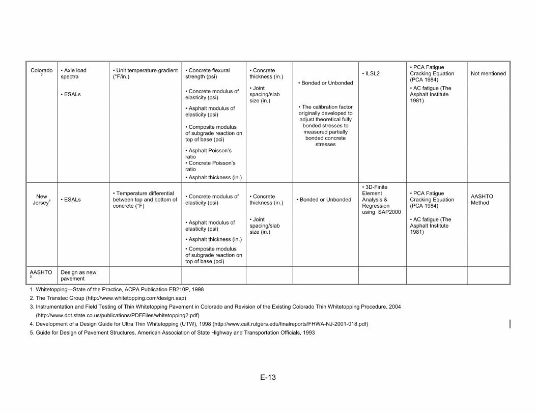
E-13

Colorado3

• Axle load spectra

• Unit temperature gradient (°F/in.)

• Concrete flexural strength (psi)

• Concrete thickness (in.)

• Bonded or Unbonded

• ILSL2 • PCA Fatigue Cracking Equation (PCA 1984)

Not mentioned

• ESALs • Concrete modulus of elasticity (psi)

• Joint spacing/slab size (in.)



• The calibration factor originally developed to adjust theoretical fully

bonded stresses to measured partially bonded concrete

stresses

• Composite modulus of subgrade reaction on top of base (pci)

• Asphalt Poisson’s ratio

• Concrete Poisson’s ratio


New Jersey4 • ESALs

• Temperature differential between top and bottom of concrete (°F)

• Concrete modulus of elasticity (psi)

• Concrete thickness (in.) • Bonded or Unbonded

• 3D-Finite Element Analysis & Regression using SAP2000

• PCA Fatigue Cracking Equation (PCA 1984)

AASHTO Method


• Joint spacing/slab size (in.)



• Composite modulus of subgrade reaction on top of base (pci)

AASHTO5

Design as new pavement

1. Whitetopping—State of the Practice, ACPA Publication EB210P, 1998 2. The Transtec Group (http://www.whitetopping.com/design.asp) 3. Instrumentation and Field Testing of Thin Whitetopping Pavement in Colorado and Revision of the Existing Colorado Thin Whitetopping Procedure, 2004 (http://www.dot.state.co.us/publications/PDFFiles/whitetopping2.pdf) 4. Development of a Design Guide for Ultra Thin Whitetopping (UTW), 1998 (http://www.cait.rutgers.edu/finalreports/FHWA-NJ-2001-018.pdf) 5. Guide for Design of Pavement Structures, American Association of State Highway and Transportation Officials, 1993

E-14

E3. MANUAL FOR THE MODIFIED ACPA GUIDE

This section describes the functions, options and equations that are part of the modified ACPA design guide software developed by Riley (2005).

E3.1. Opening Document Details

Macros must be enabled. A disclaimer is shown reading: “You Are Responsible for Results”. “The user accepts ALL responsibility for

decisions made as a result of the use of this design tool. The data represents the ‘state of the art as we know it today. American Concrete Pavement Association, its Officers, Board of Directors and Staff are absolved of any responsibility for any decisions made as a result of your use.”

E3.2. DESIGN SHEET Tab E.3.2.1. Inputs:

A project identification space is provided for project information and other information at the top of the sheet.

The failure criteria inputs are also found at the top of the sheet: o Maximum allowable percent slabs cracked Pcr in percentage (default

20%) o Desired reliability against slab cracking R in percentage (default 90%)

Traffic Distribution can be chosen from a selection of 4 different categories shown in Table E.2.

o Standard Category (default is 3 – Industrial Subdivision). A comment is made describing the possible categories and their corresponding applications. These categories are classes based on the ACPA Street Design Manual. For each category, there are load levels (Lx) preset for each axle and two axle types: single (L2=1) and tandem (L2=2).

Table E.2. Allowable Traffic Values

LR Auto Parking Lot Typical 1 Light Residential 2 Typical Collector 3 Industrial Subdivision

o Average Daily Truck Traffic ADTT (2-Way) (default is 600). o Design Life Y in years (default is 20 years). A comment is added to this

cell stating: Currently data is limited to at best 15 years, so be careful with extrapolation.”

PCC Geometry: o Thickness - Trial Thickness hc (inches) (default is 4 inches) o Slab Size - Trial Joint Spacing L (inches) (default is 48 inches) Square

slabs/joints are assumed. Concrete Properties:

o Strength - Average 28-day Third Point Flexural Strength fr (psi) (default is 750 psi)

o Stiffness - Estimated Concrete Modulus Ec (psi) (default is 4,500,000 psi)

E-15

o CTE - Estimated Coefficient of Thermal Expansion for concrete CTE (inches*10-6/in./˚F) (default is 3.8). See Table E.3 for suggested CTE values (provided as a comment).

Table E.3. Typical Coefficient of Thermal Expansion for Concrete

o Fiber-reinforcement

Fiber Type is a pull-down tab with current choices: “N/A”, “Synthetic Structural Fibers” (default), “Steel Fibers”, “Low Modulus Synthetic”, and information for three additional user-defined fiber types can be selected.

Fiber Content Wf (pounds per cubic yard) (default is 4 lb/yd3) Note that when “N/A” is chosen from the Fiber Type pull-down menu, this input does not show up.

Bituminous Properties: o Surface Preparation is a pull-down tab with current choices: “Old Asphalt

Milled & Cleaned”, “Old Asphalt Swept” (default), “New Asphalt No Prep”, “New Asphalt Milled & Cleaned”, and information for three additional user-defined surface preparations can be selected.

o Thickness - Post-milling Bituminous Thickness hac (inches) (default is 6 inches)

o Stiffness - Estimated Bituminous Resilient Modulus EAC (psi) (default is 450,000 psi). To aid in the determination of the estimated modulus, a figure of charts is hyperlinked to this input field, shown here as Figure E.1.

hart

Figure E.1. Nomograph to determine the resilient modulus of the asphalt.

Aggregate CTE (10-6/˚F) Quartz 6.6 Sandstone 6.5 Gravel 6.0 Granite 5.3 Basalt 4.8 Limestone 3.8

E-16

Project Site Properties: o k-value - Composite Modulus of Subgrade Reaction k (pci) (default is 125

pci) (At bottom of Asphalt) A comment is added to this input cell stating “This is a composite “k” value corrected from the subgrade for stone subbase, lime-stabilized, CTB, etc.” To aid in the determination of the Modulus of Subgrade Reaction (also known as the k-value), two tables are shown as Figure E.2.

Figure E.2. Nomograph to determine the composite k-value.

Temperature Gradient Considerations:

o Temperature Gradients Linear Temperature Increase Per Inch ΔTday (Daytime ˚F change

in temperature) (default 1.65 ˚F/in.). A comment is added stating that this value should be the “maximum temperature difference bottom to top sunny day. Typically from 1.5 to 2.5 ˚F per inch pavement depth”.

Percent of time Pday for the daytime temperature differential to be in effect (default is 25%).

Linear Temperature Decrease Per Inch ΔTnight (Nighttime ˚F change in temperature) (default -0.65 ˚F/in.). A comment is added for this input stating the value should be the “maximum temperature difference bottom at night. Typically from -0.5 to -2 ˚F per inch pavement depth”.

Percent of time Pnight for the nighttime temperature differential to be in effect (default is 35%).

Other o Comments o Name of person(s) performing the analysis

E-17

E.3.2.2. Calculations:

Load Repetitions are calculated as Load in kips for Single Axle and Tandem Axle repetitions. The repetition values come from the TRAFFIC MANAGER & MISC tab.

Zero Differential ΔTzero (˚F change in temperature). This is fixed at 0 ˚F. Percent of time Pzero for the default/zero temperature differential is computed in

this cell as: = 1 - (Pday) - (Pnight) Fatigue damage in the PCC and bituminous layers FPCC and FBIT are computed

for each temperature differential (day, zero, and night) and weighted by the percentage of time the pavement is in that temperature differential. The terms

ijTOTALF , correspond from the spreadsheet i (POS = POSITIVE DIFFERENTIAL;

(ZERO = ZERO GRADIENT; NEG = NEGATIVE DIFFERENTIAL) and for material j (C = concrete; B = bitumen).

Table E.4. Fatigue Consumption for the Concrete and Asphalt at each Temperature

Gradient Fatigue Consumed Combined

Delta % of Time PCC Bit

ΔTday Pday 100/*, dayPOS

CTOTALday

PCC PFF = 100/*, dayPOS

BTOTALday

BIT PFF =

ΔTzero = 0 Pzero 100/*, zeroZERO

CTOTALzero

PCC PFF = 100/*, zeroZERO

BTOTALzero

BIT PFF =

ΔTnight Pnight 100/*, nightNEG

CTOTALnight

PCC PFF = 100/*, nightNEG

BTOTALnight

BIT PFF =

Sum of Fatigue

nightPCC

zeroPCC

dayPCCPCC FFFF ++= night

BITzero

BITday

BITBIT FFFF ++=

Bond Plane

Limits “Percent of Allowable for Conditions at Given Reliability”

from BOND PLANE MANAGER tab

A comment is added to the Bond Plane Limits cell stating “Based on 130 data points of milled old asphalt. Other data is limited. Use care outside known conditions. This is based on maximum critical load, hence is independent of repetitions.”

A statement located next to the “Sum of Fatigue” describes whether the concrete or asphalt is more significant in the fatigue control. Either “< -- Asphalt Controls” or “< -- Concrete Controls” is shown based on whether the Bit or PCC column is greater respectively.

Other information is provided on the spreadsheet is for fatigue calculated due to the load only, as shown in Table E.5.

Table E.5. Fatigue Consumption of the Concrete and Asphalt from loads only

Load Only INFO PCC Bit

100/LOADPCCF 100/LOAD

BITF

E-18

Maximum ADTT(2-Way) ADTTmax = shows X for Y years, where X is the user defined ADTT (2-Way)/ maximum sum of fatigue (either from PCC or Bit) and Y is the user defined life of the pavement

Maximum Years at Design ADTT Ymax = the user defined life (years)/ maximum sum of fatigue (either from PCC or Bit). A statement is made next to this data based on the value shown. If the value is greater than 15 years, then a warning is displayed of “< Use caution. Outside data limits”. Otherwise for the maximum years at design ADTT less than or equal to 15, the statement reads “< Within known data range.”

Design Traffic ESALs Wtx uses the AASHTO equations (E1 through E4) for ESAL calculation for rigid pavement design. Pt is the terminal serviceability, which is an unchangeable variable set to 2.25 in the program. Lx is the axle load, L2 is the axle (1 for single, 2 for tandem).

1822

46.8

7

18

52.32

46.8

2.52

log28.3)log(62.4908.5)log(

)1(10*62.11

)1()(63.3

1

5.15.45.4

log

ββ

β

β

t

x

txtx

c

c

xx

tt

GGLLLW

h

LhLL

PG

−+++−=

++=

+

++=

⎟⎠

⎞⎜⎝

⎛−−

=

(E1) (E2) (E3) (E4)

Maximum ESALs (ESALmax) computes the maximum level of ESAL traffic that the pavement is designed to withstand. See equation E5.

),max(maxBITPCC

tx

FFW

ESAL = (E5)

A note is shown in stating: “This information is primarily for reference.

Mechanistic and AASHTO methods produce much different results.” E3.3. FIBER MANAGER PROTOTYPE Tab

This spreadsheet contains the details of the fiber that are used and then

calculates adjustment factors to be used in the Design Sheet.

E.3.3.1. Inputs From Other Tabs

Fiber Code From Design – cell value equals the code of the fiber used. Fiber Content Wf (lb/yd3) value comes from the input in the Design Sheet.

E.3.3.2. Calculations

Absolute Volume of Fiber (expressed as a percent) shown in equation E6.

27462 *. * SGW V i

ftrialf =

(E6)

Interpolated adjustment (shown in equation E7) computes the estimated stress ratio for the fiber volume based on the equivalent stress ratio benefits predefined for the specific fiber type.

E-19

minminmaxminmax

min B)-B(B) - V(V) - V(V IA

trialf +=

(E7) Arbitrary Safety Cushion is a safety factor 05.0 SFf = for the fiber calculations.

This value cannot be changed by the user. Equivalent Stress Ratio Factor

o Trial factor computes the initial guess for an equivalent stress ratio factor, shown in equation E8. f

trial SFIA SR −= (E8) o Check maximum and minimum allowed factors as shown in equations E9

and E10.

min

minmin 0.1VVVV

SRSR trial

f

trialf

trial ≥<

⎩⎨⎧

= (E9)

{ }maxmax ,min BSRSR trial= (E10)

o Final Re-Adjustment Factor is the equivalent stress ratio factor shown in equation E11.

{ }0.10.1

,min0.1 max

max

<<

⎩⎨⎧

=BorSR

BSRSR

trial

trialfinal

(E11)

Table E.6 is provided on the right side of the spreadsheet listing each fiber “Type”, “Specific Gravity”, “Minimum Absolute Volume Fraction”, “Maximum Absolute Volume Fraction”, “Minimum Benefit”, and “Maximum Benefit”. The Minimum and Maximum Benefit values were determined based on experimental work by Roesler et al. (2004). There are locations in Codes 5 through 8 for the user to input their own values for a fiber type.

The Minimum and Maximum Absolute Volume Fractions are computed based on practical recommendations, expressed as percentages, and calculated based on equations E12 and E13. Recommended fiber contents are shown in Table E.7; this table and values are not shown as part of the design spreadsheet.

Table E.6. Fiber Reinforcement Properties and Benefit Values

Experimentally Determined Limit Values 2 3 4 5 6 7

Code Type Specific Gravity

SG

Minimum Volume Fraction

Vmin

Maximum Volume Fraction

Vmax

Minimum Stress Factor

Bmin

Maximum Stress Factor Bmax

1 N/A 1 100.% 1.00 1.00

2 Synthetic Structural

Fibers 0.92 0.194% 0.477% 1.24 1.39

3 Steel Fibers 7.8 0.304% 0.502% 1.10 1.46

4 Low Modulus Synthetic 0.92 0.097% 0.194% 1.00 1.05

5 Other Fiber 3 0.92 0.097% 0.194% 1.00 1.05 6 Other Fiber 4 0.92 0.097% 0.194% 1.00 1.05 7 Other Fiber 5 0.92 0.097% 0.194% 1.00 1.05 8 Other Fiber 6 0.92 0.097% 0.194% 1.00 1.05

E-20

27462min

min *. * SGW

V i

if,i =

(E12)

27462max

max *. * SGW

V i

if,i =

(E13)

Table E.7. Recommended Fiber Content Ranges

Recommended Fiber Content range

(lb/yd3) minf,W maxf,W Synthetic Structural Fibers 3 7.4

Steel Fibers 40 66

Low Modulus Synthetic 1.5 3

E3.4. BOND PLANE MANAGER Tab

Bond Prep Code is the code corresponding to the bonding type chosen by the

user in the pull-down menu on the Design Sheet. A row reprints the bond type and adjustment factor corresponding to the Bond

Prep Code. The Reliability displays R the amount provided on the DESIGN SHEET by the user. The Zero Gradient Stress Limit, Positive Gradient Stress Limit and Negative Gradient Stress Limit values come directly from their computation in the ZERO GRADIENT, POSITIVE DIFFERENTIAL, and NEGATIVE DIFFERENTIAL tabs respectively.

E.3.4.1. Calculations:

Maximum Bond Stress at Reliability maximum of the Zero Gradient, Positive Gradient or Negative Gradient stress limits, as shown in equation E14.

),,max( maxmaxmaxnightdayzero

bondσ σσσ= (E14)

Milled Iowa Shear Test on Old Asphalt at given Reliability R, calculated based on equation E15.

)1(6871201)1(3776642)1(98517387)1(41215032 234 R*.R*.R*.R*. −+−−−+−−= (E15)

Adjusted for Prep = Adjustment Factor * the Milled Iowa Shear Test Percent of Allowable for Conditions at Given Reliability = Maximum Bond Stress

at R (σbond) divided by “Adjusted for Prep” The bonding types are compared based on data and the adjustment factors are

shown in Table E.8.

E-21

Table E.8. Bonding Conditions and their Adjustment Factors

2 3

Code Type Adjustment Factor Info

1 Old Asphalt Milled & Cleaned 1 130 Data Points

2 Old Asphalt Swept 0.8 Colorado 3 New Asphalt No Prep 0.5 Colorado

4 New Asphalt Milled & Cleaned 0.4 Colorado

5 Other Prep Type 1 0.92 <--- User Option Cells 6 Other Prep Type 2 0.92 <--- User Option Cells 7 Other Prep Type 3 0.92 <--- User Option Cells

E3.5. ZERO GRADIENT Tab

The values listed at the top left-hand corner (Trial Depth through Coefficient of

Thermal Expansion) come from the DESIGN SHEET tab. The Load Safety Factor (LSF) is set at 1.0, and cannot be changed by the user at

this time. According to Huang, for small volumes of truck traffic, LSF of 1.0 is recommended.

Fiber Factor is the “EquivStressRatioFactor” calculated in the FIBER MANAGER PROTOTYPE tab. Reliability R and Slabs Cracked come from the user-defined input on the DESIGN SHEET tab. E.3.5.1. Calculations:

Neutral Axis NA of the composite bituminous and concrete structure (from Mack et al. 1997), shown in equation E16.

acACcc

accacAC

cc

hEhE

hhhEhE

NA+

⎟⎠⎞⎜

⎝⎛ ++

=22

)( 2

(E16)

Equivalent moment of inertia Ie, calculated in equation E17, for the composite bituminous and concrete structure (from Mack et al. 1997).

23

23

)2

(12

)()

2(

12)(

123 accacAC

acACccc

cce

hNAhhE

hEhNAhE

hE)e/(Eh^I +−++−+==

(E17) Equivalent characteristic length le (Poisson’s ratio for concrete assumed to be

0.15) (from Mack et al. 1997), calculated according to equation E18. 250

2 )1501(

.e

e *k.I

l ⎟⎟⎠

⎞⎜⎜⎝

⎛

−=

(E18)

Length of full bonding stress lb is computed based on equation E19.

2e

bl

l = (E19)

Combined and Load Only Fatigue values (in percent) for Total Concrete Fatigue Used ZERO

CTOTALF , and LOADPCCF ; values (in percent) for Total Asphalt Fatigue Used

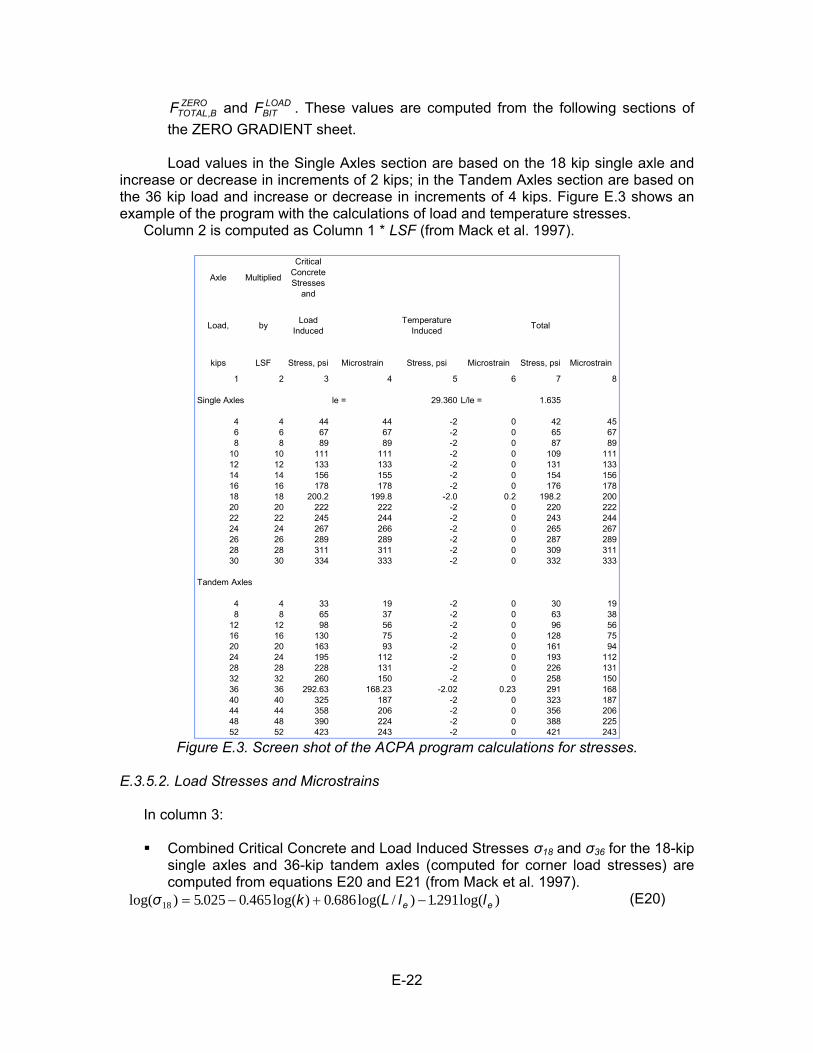
E-22

ZEROBTOTALF , and LOAD

BITF . These values are computed from the following sections of the ZERO GRADIENT sheet. Load values in the Single Axles section are based on the 18 kip single axle and

increase or decrease in increments of 2 kips; in the Tandem Axles section are based on the 36 kip load and increase or decrease in increments of 4 kips. Figure E.3 shows an example of the program with the calculations of load and temperature stresses.

Column 2 is computed as Column 1 * LSF (from Mack et al. 1997).

Axle Multiplied

Critical Concrete Stresses

and

Load, by Load Induced

Temperature Induced Total

kips LSF Stress, psi Microstrain Stress, psi Microstrain Stress, psi Microstrain

1 2 3 4 5 6 7 8

Single Axles le = 29.360 L/le = 1.635

4 4 44 44 -2 0 42 456 6 67 67 -2 0 65 678 8 89 89 -2 0 87 89

10 10 111 111 -2 0 109 11112 12 133 133 -2 0 131 13314 14 156 155 -2 0 154 15616 16 178 178 -2 0 176 17818 18 200.2 199.8 -2.0 0.2 198.2 20020 20 222 222 -2 0 220 22222 22 245 244 -2 0 243 24424 24 267 266 -2 0 265 26726 26 289 289 -2 0 287 28928 28 311 311 -2 0 309 31130 30 334 333 -2 0 332 333

Tandem Axles

4 4 33 19 -2 0 30 198 8 65 37 -2 0 63 38

12 12 98 56 -2 0 96 5616 16 130 75 -2 0 128 7520 20 163 93 -2 0 161 9424 24 195 112 -2 0 193 11228 28 228 131 -2 0 226 13132 32 260 150 -2 0 258 15036 36 292.63 168.23 -2.02 0.23 291 16840 40 325 187 -2 0 323 18744 44 358 206 -2 0 356 20648 48 390 224 -2 0 388 22552 52 423 243 -2 0 421 243

Figure E.3. Screen shot of the ACPA program calculations for stresses.

E.3.5.2. Load Stresses and Microstrains

In column 3: Combined Critical Concrete and Load Induced Stresses σ18 and σ36 for the 18-kip

single axles and 36-kip tandem axles (computed for corner load stresses) are computed from equations E20 and E21 (from Mack et al. 1997).

)log(2911)/log(6860)log(46500255)log( 18 ee l.lL.k..σ −+−= (E20)

E-23

All other values in the single axle section compute the stress as the corresponding column 2 values for that given load divided by 18 kips and multiplied by the stress for 18-kip single axle load.

)/(0880)log(9630)/log(3951)log(55908984)log( 36 eee lL.l.lL.k..σ −−+−= (E21) All other values in the tandem axle section compute the stress as the

corresponding column 2 values for that given load divided by 36 kips and multiplied by the stress for 36-kip tandem axle load.

These equations come from concrete stresses at a corner (from Mack et al. 1997).

In column 4:

Critical load-induced asphalt microstrains (με) are computed at a joint (from Mack et al. 1997). For 18-kip single axle load, the με18 is computed from the following equation E22,

ee l.lL.k..)(μ 0370)/log(2990)log(92702675log 18 −+−=ε (E22) where all other values in the single axle section compute the microstrain as the corresponding column 2 load value divided by 18 kips and multiplied by the με for 18-kip single axle load.

For 36-kip tandem axle load, the με36 is computed from the following equation E23 (from Mack et al. 1997),

ee l.lL.k.-.μ 0280)/log(7860)log(8910076)log( 36 −−=ε (E23) where all other values in the tandem axle section compute the microstrain as the corresponding column 2 load value divided by 36 kips and multiplied by the με for 36-kip tandem axle load.

E.3.5.3. Temperature Stress and Microstrain

For column 5: Temperature Induced Stress σT at the top of the concrete slab at

the corner is computed according to equation E24 (from Mack et al. 1997). )/(38218)(496303728 eT lL.TCTE*..σ −Δ−= (E24)

For column 6: The strain at the top of the AC layer (με) from temperature is computed according to equation E25 for a joint case.

)/(69217)*(131269828 elL.TCTE..με +Δ+−= (E25) For column 7: Total stress σTOTAL is the sum of Column 3 and Column 5 as

shown in equation E26, where xσ is either 18σ or 36σ .

TxTOTAL σσσ += (E26) For column 8: Total microstrain is the sum of Column 4 and Column 6.

Column 9 comes directly from the values on the Design Sheet for expected

repetitions at each load level. Figure E.4 shows an example of the fatigue calculations.

E-24

Axl

eC

oncr

ete

Fatig

ue

Anal

ysis

Asp

halt

Fatig

ue

Anal

ysis

Bon

d P

lane

C

alcu

latio

ns

Load

,E

xpec

ted

Con

cret

eA

llow

able

Fatig

ueA

spha

ltA

llow

able

Fatig

ueEs

timat

ed B

ond

Pla

ne

Con

cret

e S

tress

C

ompr

essi

ve

Estim

ated

Con

cret

e M

icro

Stra

in a

t Rel

iabi

lity

Estim

ated

A

spha

lt St

ress

In

fers

Bon

d Pl

ane

Stre

ss

kips

Rep

etiti

ons

Stre

ss R

atio

Rep

etiti

ons,

NP

erce

nt, %

mic

rost

rai

nR

epet

ition

s, N

Per

cent

, %

19

1011

1213

1415

Zsco

re A

djus

tmen

tS

ingl

e Ax

les

1.28

1551

566

40

0.05

7un

limite

d0.

045

290,

443,

920

0.0

18.1

4.0

60

0.08

6un

limite

d0.

067

76,9

06,0

530.

027

.66.

18

00.

116

unlim

ited

0.0

8929

,922

,367

0.0

37.1

8.3

100

0.14

6un

limite

d0.

011

114

,381

,059

0.0

46.6

10.4

1239

8,62

40.

175

unlim

ited

0.0

133

7,90

1,13

55.

056

.112

.56

1410

4,52

90.

205

unlim

ited

0.0

156

4,76

1,16

72.

265

.614

.67

1669

,686

0.23

5un

limite

d0.

017

83,

069,

880

2.3

75.1

16.7

818

55,0

790.

264

unlim

ited

0.0

200

2,08

4,39

62.

684

.618

.88

2035

,763

0.29

4un

limite

d0.

022

21,

474,

191

2.4

94.1

20.9

922

17,1

920.

324

unlim

ited

0.0

244

1,07

7,61

31.

610

3.6

23.0

1024

11,4

100.

353

unlim

ited

0.0

267

809,

488

1.4

113.

125

.111

263,

898

0.38

3un

limite

d0.

028

962

2,15

90.

612

2.6

27.3

1228

1,86

20.

413

unlim

ited

0.0

311

487,

598

0.4

132.

129

.413

3098

60.

442

unlim

ited

0.0

333

388,

617

0.3

141.

631

.514

Tand

em A

xles

40

0.04

1un

limite

d0.

019

Unl

imite

d0.

013

.02.

98

00.

084

unlim

ited

0.0

3851

0,19

4,45

30.

026

.96.

012

00.

127

unlim

ited

0.0

5613

5,23

3,80

00.

040

.89.

116

217,

555

0.17

1un

limite

d0.

075

52,6

43,7

660.

454

.712

.25

2018

8,20

90.

214

unlim

ited

0.0

9425

,309

,166

0.7

68.6

15.2

724

158,

863

0.25

7un

limite

d0.

011

213

,908

,079

1.1

82.4

18.3

828

265,

472

0.30

1un

limite

d0.

013

18,

382,

160

3.2

96.3

21.4

1032

226,

950

0.34

4un

limite

d0.

015

05,

405,

210

4.2

110.

224

.511

3612

3,18

80.

387

unlim

ited

0.0

168

3,67

0,36

53.

412

4.1

27.6

1240

46,6

690.

431

unlim

ited

0.0

187

2,59

6,05

11.

813

8.0

30.7

1444

17,5

420.

474

unlim

ited

0.0

206

1,89

7,78

40.

915

1.9

33.7

1548

6,37

30.

518

unlim

ited

0.0

225

1,42

5,65

80.

416

5.7

36.8

1752

2,60

60.

561

1,81

0,72

30.

124

31,

095,

782

0.2

179.

639

.918

Tota

l Con

cret

e Fa

tigue

, %

0.1

Tota

l Asp

halt

Fati

35.3

5.46

7513

0917

.963

0211

517

.963

0211

5

g10(

le)

69.6

2967

38

Figu

re E

.4. S

cree

n sh

ot o

f the

fatig

ue a

nd b

ond

plan

e ca

lcul

atio

ns.

E-25

E.3.5.4. PCC Fatigue Calculations

Concrete Fatigue Analysis is shown in Columns 10-12. Column 10: Concrete stress ratio computed in equation E27.

MORSR TOTAL

PCCσ

= (E27)

Column 11: Allowable Repetitions for Concrete Fatigue NPCC uses a function called “Reps” and is a function of Concrete Stress Ratio SRpcc, Reliability R ,Slabs Cracked Pcr, and equivalent stress ratio factor SRf. The equivalent stress ratio factor is shown in equation E28. Equations E29 and E30 are used in the function Reps. As part of the function, a couple checks are made first as shown as follows:

o Checks: If SRPCC <0, then SRPCC = 0.000001 If SRf <1, then SRf =1.0

217.024.10

0112.0*)log(

log

5.0*)1(

1*

⎥⎥⎦

⎤

⎢⎢⎣

⎡−=

−−=

=

− RSRN

PRR

SRSR

SR

totalPCC

cr

f

PCCtotal

(E28) (E29) (E30)

If (log NPCC )>7, then “unlimited” is displayed in column 11, otherwise NPCC is shown.

Column 12: Concrete Fatigue Percent

When the value for Allowable Repetitions in Column 11 displays “unlimited”, then

a value of 0.0 is shown. Otherwise the Fatigue percent is computed to be Expected Repetitions (Column 9) divided by Allowable Repetitions (Column 11)*100.

The Total Concrete Fatigue Used (in percent) is computed as the sum of column 12 values.

E.3.5.5. AC Fatigue Calculations

Asphalt Fatigue Analysis is shown in Columns 13-15.

Column 13: Asphalt Microstrain values from Column 8 are re-presented here. Column 14: Allowable Repetitions for Asphalt Fatigue NBIT is computed using the

function called “BitReps” dependent on Asphalt Microstrain, EAC, Pcr, and R. These calculations are shown in equations E31 and E32. Again a check is made first as follows:

o Checks: If μεx <0, then μεx = 0.00001

⎟⎠

⎞⎜⎝

⎛−−+−=

−=

310log854.0)log(291.31598.16)'1log(0924.0log

)1('

ACxBIT

cr

ERN

RPR

με

(E31) (E32)

E-26

If (log NBIT )>9, then “unlimited” is displayed in column 14, otherwise NBIT is shown.

Column 15: Asphalt Fatigue Percent When the value for Allowable Repetitions in Column 14 displays “unlimited”, then


The Total Asphalt Fatigue Used (in percent) is computed as the sum of column 15 values. E.3.5.6. Bond Plane Calculations

A term called the Zscore adjustment is computed as seen in equation E33. This is the absolute value of the inverse standard normal cumulative distribution of the probability (1 – Reliability).

)1(Adjustment Zscore 1 R−Φ= − (E33)

Estimated Bond Plane Concrete Stress (compressive or tensile) is computed according to equation E34.

))Adjustment e0.32(Zscor(1.57*360.-(1*Stress Total +=c

c

h-NA)(h

)* (E34)

Estimated Concrete Microstrain at Reliability = (Estimated Bond Plane) / (Ec)*106 Estimated Asphalt Stress Infers Bond Plane Stress

When Expected Repetitions (Column 9) is greater than 0 for that load level, then

the value shown is the (Estimated Concrete Microstrain) *EAC / 106. Calculations are unlabelled at the bottom of the Estimated Asphalt Stress

column:

The minimum Estimated Asphalt Stress is computed The maximum Estimated Asphalt Stress is computed The maximum of either |min Estimated Asphalt Stress| or |max Estimated

Asphalt Stress| Iowa Shear Strength = -15032.412(1-R)4 + 17387.985(1-R)3 - 6642.377(1-R)2 +

1201.687(1-R)

E.3.5.7. Load Only Fatigue Calculations

Similar analysis is performed for each load level without temperature effects.

Column 16: Expected Repetitions values are represented from Column 9. Concrete Fatigue Analysis is Columns 17-19:

Column 17: Concrete stress Ratio = Total Stress (Column 3) divided by the Concrete Modulus of Rupture MOR.

Column 18: Allowable Repetitions for Concrete Fatigue computed using the Reps function similar to column 11.

Column 19: Concrete Fatigue Percent.

E-27

When the value for Allowable Repetitions in Column 18 displays “unlimited”, then a value of 0.0 is shown. Otherwise the Fatigue percent is computed to be Expected Repetitions (Column 16) divided by Allowable Repetitions (Column 18)*100.

The Total Concrete Fatigue Used for Load Only (in percent) is computed as the sum of column 19 values.

Asphalt Fatigue Analysis is Columns 20-22:

Column 20: Asphalt Microstrain values from Column 4 are re-presented here. Column 21: Allowable Repetitions for Asphalt Fatigue is computed using the

BitReps function similar to column 14. Column 22: Asphalt Fatigue Percent

When the value for Allowable Repetitions in Column 21 displays “unlimited”, then


The Total Asphalt Fatigue Used (in percent) is computed as the sum of column 22 values. E3.6. POSITIVE DIFFERENTIAL and NEGATIVE DIFFERENTIAL Tabs

See Zero Gradient for description of inputs. The Load Only values are not shown (only Combined Fatigue percentages

shown) here since this Positive Differential tab and the Negative Differential tab are used to analyze different Temperature Differentials seen in the pavements. E3.7. TRAFFIC MANAGER & MISC Tab

The following Figure E.5 shows the Traffic Manager and Miscellaneous Tab.

This spreadsheet computes the traffic distribution.

E-28

Design Life 20 YearsADTT (2 way) 600

Axle Cat. 3

TRAFFIC INPUTS

Load Kips ExpectedSingle Axle Repetitions Axle Load LR 1 2 3

4 0 Single Axle6 0 4 846.15 1693.318 0 6 369.97 732.28

10 0 8 283.13 483.1 233.612 398,624 10 257.6 204.96 142.714 104,529 12 103.4 124 116.76 182.0216 69,686 14 39.07 56.11 47.76 47.7318 55,079 16 20.87 38.02 23.88 31.8220 35,763 18 11.57 15.81 16.61 25.1522 17,192 20 4.23 6.63 16.3324 11,410 22 0.096 2.6 7.8526 3,898 24 1.6 5.2128 1,862 26 0.07 1.7830 986 28 0.85

30 0.45Tandem Axles Tandem Axle

4 0 4 15.12 31.98 0 8 39.21 85.59 47.01

12 0 12 48.34 139.3 91.1516 217,555 16 72.69 75.02 59.25 99.3420 188,209 20 64.33 57.1 45 85.9424 158,863 24 42.24 39.18 30.74 72.5428 265,472 28 38.55 68.48 44.43 121.2232 226,950 32 27.82 69.59 54.76 103.6336 123,188 36 14.22 4.19 38.79 56.2540 46,669 40 7.76 21.3144 17,542 44 1.16 8.0148 6,373 48 2.9152 2,606 52 1.19

Figure E.5. Example of the traffic distribution calculation.

F-1

APPENDIX F. THERMAL STRESS ANALYSIS

Several challenges in ensuring an ultra-thin whitetopping (UTW) pavement meets the service life objective are preserving bond between the concrete and existing asphalt concrete layer, and maintaining adequate load transfer across the joints. Since no man-made load transfer devices exist across the contraction joints, the crack width or joint opening must be minimized to maintain aggregate interlock. Several ways to minimize joint opening include smaller slab sizes and selecting concrete mixtures with low heat of hydration, low drying shrinkage potential, or with the inclusion of fiber-reinforcement. Selection of a small slab size will only promote good load transfer if a working crack exists at early ages. Several UTW projects completed at the University of Illinois in the summer of 2006 and 2007 indicated that many of the contraction joints did not crack initially. In fact, the initial joint cracks occurred at every 5 to 8 joints (for 4 x 4 ft panels). The result of this large crack spacing was wider openings at these initial crack locations and reduced load transfer (see FWD results in Appendix B for UIUC Parking Lot E-15). Cracks at other locations eventually propagated, but the load transfer efficiency (LTE) across these cracks were dramatically higher than the initial cracks. The primary objective of this field, laboratory, and analytical study was to determine if the initial crack spacing at early ages (e.g., 24 hours) can be approximately predicted for UTW sections, and if it is possible to promote additional cracks to propagate at early ages. One additional factor, which has made it more difficult to propagate cracks at early ages, is the addition of fibers, which increase the crack propagation resistance of the concrete. The nonlinear mechanical behavior of the fiber reinforcement was difficult to account for in conjunction with the selected nonlinear elastic fracture mechanics model presented in this study.

This appendix summarizes the theoretical thermal stress calculations for ultra-thin whitetopping and presents laboratory material parameters and field temperature measurements on a recently constructed UTW project. There are two types of thermal stresses concerned, namely axial thermal stress due to uniform temperature change in the slab, and curling stress, due to temperature differential through the slab thickness; for simplicity, only linear temperature differentials throughout the slab are considered. Field and laboratory data are presented for several concrete mixture designs at early ages. Finally a discussion is presented to interpret the field observations and results of the analytical model. F.1. SOLUTION METHODS FOR AXIAL THERMAL STRESS

To calculate the axial thermal stress due to uniform temperature change in the slab, two mechanistic-based methods are used. The first one was developed using one-dimensional elasticity theory with a bilinear slab-base friction assumption (Zhang and Li, 2001). This one-dimensional model was modified to predict the time-dependent joint opening in jointed plain concrete pavement (JPCP) due to climatic loadings (Roesler and Wang, 2008). The solution method generates a spatially dependent axial thermal stress. The one-dimensional model takes slab geometries into consideration, such as slab thickness h and length L; in addition the model includes a few other material properties, such as the elastic modulus of the concrete E, the steady-state slab-base frictional stress τ0, and its corresponding slab slippage δ0, where τ0 and δ0 can be determined from a field test. This solution method is abbreviated as the “Bilinear Model” in this document.

A second method was introduced by Westergaard in 1926 and is based on a two-dimensional elasticity theory. Only the maximum axial thermal stress in the interior area of a large slab can be calculated. As expected, the derived formula is independent of slab geometric conditions.

F-2

To facilitate the introduction of the Bilinear Model, the underlying bilinear slab-base interfacial restraint model is presented first (Roesler and Wang, 2008). F.1.1. Slab-Base Interfacial Restraint

Let x be the direction along the Portland cement concrete (PCC) slab length, z be the direction along the PCC slab thickness, where z is measured positive downward and z = 0 is at the mid-depth of slab. The ends of the slab are located at x = 0 and x = L. It is assumed that no displacement occurs at the mid-span of the slab x = L/2, thus only half of the slab (0 < x < L/2) is analyzed. The coordinate system is shown in Figure F.1.

The slab-base friction interaction serves as a restraint to slab movement, thus proper characterization of this friction is critical for accurately predicting the axial thermal stress in the concrete slab. Field push-off test results suggest that the stress-slippage behavior of a slab-base interface can be satisfactorily approximated by a bilinear function as presented in equation F1 below (Rasmussen and Rozycki, 2001; Wimsatt et al. 1987).

⎪⎪⎪

⎩

⎪⎪⎪

⎨

⎧

<−<−

<<

≤

=

000

00

0

0

δτ

δτ

δδτ

τ

)( if

)(0 if

)( if )(

)(

0

xu

xu

xuxu

x . (F1)

where τ(x) is the slab-base interfacial friction at x (MPa), and a stress sign convention is applied (Timoshenko and Goodier, 1970); τ0 is the steady-state friction (MPa); δ0 is the slippage (displacement) corresponding to the friction of τ0 (mm); u(x) is the average displacement through the PCC slab thickness (mm). In cases where u(x) > 0, the PCC slab contracts, and where u(x) < 0, the PCC slab expands for 0 < x < L/2.

Equation F1 is plotted in Figure F.2. Table F.1 lists some typical values of τ0 and δ0 for different base types. The largest slab-base restraint τ0 and smallest threshold displacement δ0 values exist in cement stabilized base compared to those in other types of base. This is one of the main reasons why JPCP with a semi-rigid base are susceptible to environment-induced cracking at early ages.

h

L/2

x

z

h

L/2

x

z

L/2

x

z Figure F.1. Coordinate system used in the slab-base interfacial restraint model.

F-3

u(x)0 δ0

τ0

u(x)0 u(x)00 δ0

τ0

Figure F.2. The bilinear slab-base restraint model.

Table F.1. Typical Slab-Base Frictional Restraint Values for Different Types

of Bases (after Rasmussen and Rozycki, 2001) Base Type τ0 (MPa) δ0 (mm)

Dense-Graded HMA (Rough) 0.069 0.25 Dense-Graded HMA (Smooth) 0.035 0.51 Cement Stabilized 0.103 0.025 Lime Treated Clay 0.010 0.76 Natural clay 0.007 1.00 Granular 0.014 0.51

F.1.2. Maximum Thermal Stress, mσ Based on Bilinear Model

Equation F1 and Figure F.2 suggest that there are two cases for which axial thermal

stress development should be studied. The maximum axial thermal stress σm for each case is listed below.

• Case 1 occurs when 00 δ≤)(u , thus

⎥⎦

⎤⎢⎣

⎡−Δ⋅−=

)/cosh( 211

LTE avem β

ασ . (F2)

• Case 2 occurs when 00 δ≥)(u and 00 δ=)(xu , thus

)).(cosh()).(cosh( 000

2

0 501

5011

xLxE

xLTE avem −

+⎥⎦

⎤⎢⎣

⎡−

−Δ⋅−=β

δββ

ασ . (F3)

Here, E and μ are the modulus of elasticity and Poisson’s ratio of concrete, respectively;

ΔTave is the temperature difference between uniform (or average) temperature at time t in the slab and slab setting temperature, where the method for calculating average temperature in the slab is presented in Section F.2; α is the coefficient of thermal expansion of concrete; h is the

slab thickness ;0

0

δτ

βEh

= ; x0 is the coordinate value of x where the displacement u equals δ0

F-4

(x0 can be numerically determined using equation F4 via a nonlinear equation solver, such as Newton-Raphson iterative method described by Burden and Faires, 2001).

[ ] )(

)(

00

00

002

01

xLx

xLx

ave eeeeTx −−−

−−−

+−

Δ⋅+−= ββ

ββ

αδββ

δ (F4)

F.1.3. Westergaard’s Axial Thermal Stress Formula

Westergaard’s formula for calculating the maximum thermal stress, assuming an infinite slab length, is given in equation F5 (Westergaard 1926) as

μα

σ−Δ⋅

=1

avem

TE (F5)

As mentioned above, the Westergaard solution is the maximum axial thermal stress

induced in the central part of a large slab, where horizontal displacements due to uniform temperature changes are assumed to be fully resisted by the slab-base frictional restraint. Equation F5 always over-estimates the axial thermal stress value since finite slab sizes exist in reality. The Westergaard axial thermal stress serves as the upper bound for axial thermal stresses calculated using other mechanistic models and therefore, should be used with caution. F.2. CURLING STRESS DUE TO LINEAR TEMPERATURE DIFFERENTIAL THROUGH

SLAB THICKNESS

Westergaard’s curling stress formula for the case of a slab having infinite width and finite length L can be applied (Westergaard 1926). The maximum tensile or compressive stress σ at the top of slab in the middle of slab length is (derived from Westergaard 1926)

⎥⎦⎤

⎢⎣⎡

++

−=λλ

λλλλσσ22

210 sinhsin)sinhcoscosh(sin

, (F6)

where )( μ

ασ

−Δ⋅

=120

cTE;

8lL

=λ ; 42

3

112 kEhl

)( μ−= ; and ΔTc is the temperature difference

between the top and the bottom of slab, under the assumption of a linear temperature gradient through the thickness; and k is the modulus of subgrade reaction.

The linear temperature difference between the top and the bottom of slab ΔTc(t), can be extracted from a measured nonlinear temperature profile using the concept of an equivalent linear temperature component (Ioannides and Khazanovich, 1998). Given the measured temperature profile through the thickness of slab, T(z,t), the average temperature through the thickness of slab, Tave(t), which is needed in the axial thermal stress calculation can be approximated in equation F7 using the mean-value theorem of integration in calculus.

∫−=2

2

1 /

/),()(

h

have dztzTh

tT . (F7)

Also, ΔTc(t) is given in equation F8 below (Roesler and Wang, 2008) as

∫−−=−−=Δ2

22

1222

/

/),(),(),()(

h

hLLc dtTh

thTthTtT ξξξ , (F8)

F-5

where TL is the equivalent linear temperature component. F.3. THERMAL STRESS CALCULATIONS

The main inputs for the calculation of thermal stresses based on the above methods are listed as: temperature profile, setting temperature, elastic modulus, base parameters, and the soil k-value. F.3.1. TEMPERATURE PROFILE

The temperature profile through the thickness of slab is critical in the thermal stress development at early ages. In this study, measured field temperature in a 4.5-inch slab cast under full sunshine conditions at University of Illinois campus in the summer of 2007 was used. Since the temperature profile in the slab during the first 24 hours plays an important role in selecting the appropriate saw-cutting for UTW (including saw-cut timing, joint spacing, etc), slab temperature data measured at different depths for times t = 6, 8, 10, 12, and 24 hours after the slab was cast was used and listed in Table F.2. Furthermore, the average temperature and equivalent linear temperature differential through the thickness of slab calculated using equations F7 and F8, respectively are listed in Table F.3.

Table F.2. Measured Concrete Slab Temperature at Different Depths (°C)

Time After Slab Cast (hrs) Surface 1 in. 2 in. 4.5 in.

6 47.73 48.39 48.41 45.06 8 44.68 45.18 45.56 44.56

10 39.41 40.97 42.10 42.72 12 35.50 36.99 38.22 39.69 24 31.32 31.33 31.36 31.44

Table F.3. Calculated Average Temperature and Linear Temperature Differential (°C)

Time After Slab Cast (hrs) Mean Temperature ΔT (Ttop – Tbottom)

6 47.03 4.87 8 44.99 0.72

10 41.79 -3.62 12 38.22 -5.07 24 31.38 -0.18

F.3.2. SETTING TEMPERATURE

The setting temperature is assumed to be 50 °C, and inferred to occur at t = 5 hours

after the slab was cast, based on the observation of temperature profile measured at every 15-minute interval. F.3.3. ELASTIC MODULUS OF CONCRETE

The elastic modulus of concrete E is an important material parameter used in any elasticity theory-based thermal stress formulation. In this study, elastic moduli of six different concrete mixtures tested in the laboratory were used, and their measured values are given in Table F.4. The elastic moduli for the concrete mixtures were measured in the laboratory as part

F-6

of research done by Gaedicke et al. (2007), based on concrete mixtures for airport pavement applications, except Mix_3 and Mix_11, which were based on a high early strength UTW pavement built in Anna, IL and a CRCP pavement on the Dan Ryan expressway, respectively. Note the airport concrete mixture nomenclature in Table F.4 (e.g., 555.44) stands for the 555 lb/yd3 of cementitious materials, 0.44 water to cement ratio, and ‘st’ means a 1-inch maximum aggregate size was used instead of 1.5 inches.

Table F.4. Elastic Modulus of Concrete at Early Ages (MPa)

Mixture 6 hours 8 hours 10 hours 12 hours 24 hours Mix_3 (Anna, IL) 7, 331 9, 468 11, 452 13, 283 21, 049 Mix_11 (Dan Ryan) 3, 360 4, 480 5, 601 6, 721 13, 441 555.44 1, 635 4, 542 7, 766 11, 820 16, 843 555.44st 1, 196 3, 322 5, 679 8, 643 12, 316 688.38 1, 180 3, 277 5, 603 8, 528 12, 152 688.38st 1, 368 3, 800 6, 496 9, 888 14, 090

F.3.4. BASE PARAMETERS

The parameters used in the bilinear slab-base restraint model for concrete placed on an asphalt layer are: τ0 = 0.052 MPa and δ0 = 0.38 mm. F.3.5. K-VALUE

The k-value or modulus of subgrade reaction used in Westergaard’s curling stress formula is assumed to be 100 psi/in.

F.3.6. MAXIMUM AXIAL THERMAL STRESS

The maximum axial thermal stress are given in Table F.5 for different joint spacing calculated using the Bilinear Model for Mix_3 (Anna, IL), along with those based on Westergaard’s formula, which is independent of joint spacing. Table F.5 demonstrates that the maximum axial thermal stress only varies slightly with large joint spacings from 120 ft to 240 ft. Thus, only the maximum axial thermal stress based on the Bilinear Model for L were taken between 12 ft and 120 ft for the rest of mixture analyses considered in this study. Thermal stresses for joint spacing less than 12 ft were not calculated since the tensile stresses were very small.

F-7

Table F.5. Maximum Axial Thermal Stress Based on Bilinear Model for Mix_3 (Anna) (MPa)

Joint Spacing L (ft) Time Elapsed (hrs) 6 8 10 12 24

12 0.0501 0.0882 0.148 0.217 0.357 20 0.104 0.193 0.335 0.502 0.837 24 0.128 0.242 0.428 0.648 1.073 28 0.148 0.286 0.512 0.785 1.304 30 0.156 0.305 0.551 0.848 1.417 40 0.187 0.380 0.707 1.113 1.956 60 0.214 0.453 0.872 1.412 2.849 80 0.222 0.478 0.935 1.537 3.431 100 0.225 0.487 0.959 1.587 3.748 120 0.225 0.490 0.968 1.607 3.907 140 0.225 0.491 0.971 1.615 3.984 160 0.226 0.491 0.972 1.618 4.021 180 0.226 0.491 0.973 1.619 4.040 200 0.226 0.491 0.973 1.620 4.048 220 0.226 0.491 0.973 1.620 4.053 240 0.226 0.491 0.973 1.620 4.055 Westergaard’s Result 0.265 0.578 1.145 1.906 4.772

Table F.6 lists the curling stresses at the top of the slab for different joint spacing values

for Mix_3. As expected, Table F.6 shows that Westergaard’s curling stress values remain unchanged in the first three or four decimal places when L was greater than 40 ft (L/l → ∞ ). Therefore, only the curling stresses for L ranging from 12 ft to 40 ft for the other mixtures were considered for other mixtures.

Table F.6. Curling stress for Mix_3 (Anna) (MPa) Joint Spacing

L (ft) Time Elapsed (hrs)

6 8 10 12 24 12 -0.236 -0.0449 0.268 0.429 0.0222 20 -0.219 -0.0425 0.259 0.424 0.0249 24 -0.216 -0.0417 0.253 0.412 0.0231 28 -0.217 -0.0416 0.251 0.408 0.0226 30 -0.217 -0.0417 0.251 0.408 0.0225 40 to 240 -0.217 -0.0418 0.252 0.410 0.0226

F.4. ANALYSIS OF SAW-CUTTING PATTERN

Table F.7 lists the nominal strength of concrete slab (σN) for the Mix_3 (Anna) mixture versus the notch depth-to-slab thickness ratio (a/d), where a is the notch depth and d is the slab thickness. σN is calculated using Bazant’s size effect model and measured concrete fracture properties (KIC and cf) at several ages. The detailed explanation of this model is contained in the research paper by Gaedicke et al. (2007).

F-8

Table F.7. Nominal Strength (σN) for Mix_3 (MPa) Time (hrs)

Notch Depth-to-Slab Thickness Ratio 0.0 0.1 0.2 0.3 0.4 0.5 0.6 0.7 0.8 0.9 1.0

6 0.268 0.301 0.284 0.267 0.243 0.212 0.178 0.145 0.116 0.092 0.0728 0.461 0.671 0.649 0.621 0.571 0.499 0.417 0.337 0.268 0.211 0.16510 1.279 1.026 0.874 0.771 0.682 0.595 0.507 0.422 0.344 0.275 0.219

Given the nominal strength of concrete slab (σN) and maximum tensile thermal stress σ for a fixed joint spacing at a particular time (Tables F.5 plus F.6 stresses), the saw-cut depth to slab thickness ratio (a/d) can be determined by setting σ equal to σN from Table F.7 for Mix_3 (Anna). A set of notch depth ratios required for equilibrating the nominal strength of the concrete to the maximum tensile stress for various joint spacing at different saw-cutting times are given in Table F.8 for Mix_3 (Anna).

Table F.8. Saw-Cut Depth to Slab Thickness Ratio (a/d) for Slab Made by Mix_3 for Different Joint-Spacing

Joint spacing

L (ft)

Concrete Ages 6 hrs 8 hrs 10 hrs

Tensile Stress a/d Tensile Stress a/d Tensile Stress a/d 12 0.28 (Bottom) 0.043 Too early 0.416 0.7 20 0.323 (Bottom) 0.151 1.0 0.594 0.5 24 0.344 (Bottom) 0.200 0.9 0.681 0.4 28 0.365 (Bottom) 0.244 0.85 0.763 0.3 30 0.373 (Bottom) 0.263 0.8 0.802 0.2540 0.404 (Bottom) 0.338 0.7 0.959 0.1560 0.431 (Bottom) 0.411 0.6 1.124 0.05

Note that the tensile stress in Table F.8 is the superposition of axial thermal stress and maximum tensile curling stress; the tensile stress is calculated at the top of slab, except at t = 6 hours where it is greatest at the bottom of the slab due to daytime curling stresses. In the case of maximum tensile stresses at the bottom of the slab, no saw-cut depth suggestion is made.

Likewise, the nominal strengths of concrete slab (σN) made by the other mixtures at different notch depth-to-slab thickness ratios (a/d) are given in Tables F.9, F.11, F.13, F.15, and F.17, and the corresponding saw-cutting (a/d) ratio based on critical tensile stress (thermal) are given in Tables F.10, F.12, F.14, F.16, and F.18, respectively.

Table F.9. Nominal Strength (σN) for Mix_11 (Dan Ryan) (MPa) Time (hrs)


6 0.035 0.032 0.029 0.026 0.023 0.020 0.017 0.014 0.011 0.009 0.0078 0.272 0.092 0.067 0.055 0.048 0.042 0.036 0.030 0.025 0.021 0.01610 0.300 0.156 0.119 0.100 0.087 0.075 0.065 0.055 0.045 0.037 0.029

F-9

Table F.10. Saw-cut Depth to Slab Thickness Ratio (a/d) for Mix_11 (Dan Ryan) for Different Joint Spacings

Joint spacing

L (ft)


Tensile Stress a/d Tensile Stress a/d Tensile Stress a/d 12 0.148 (Bottom) 0.0541 0.3 0.265 0.05 20 0.170 (Bottom) 0.120 0.08 0.380 Too late 24 0.180 (Bottom) 0.144 0.07 0.429 Too late 28 0.187 (Bottom) 0.162 0.06 0.469 Too late 30 0.190 (Bottom) 0.169 0.06 0.486 Too late 40 0.198 (Bottom) 0.193 0.04 0.542 Too late 60 0.203 (Bottom) 0.208 0.04 0.585 Too late

Table F.11. Nominal strength (σN) for Mix 555.44 (MPa) Time (hrs)


6 0.058 0.053 0.051 0.048 0.044 0.038 0.032 0.026 0.021 0.016 0.013 8 0.314 0.275 0.252 0.231 0.209 0.182 0.154 0.126 0.102 0.081 0.064 10 0.594 0.498 0.443 0.401 0.358 0.313 0.265 0.219 0.177 0.141 0.112

Table F.12. Saw-cut Depth to Slab Thickness Ratio (a/d) for Mix 555.44 for Different Joint

Spacings Joint

spacing L (ft)


Tensile Stress a/d Tensile Stress a/d Tensile Stress a/d 12 0.0801 (Bottom) 0.0541 Too early 0.325 0.45 20 0.0913 (Bottom) 0.121 0.70 0.467 0.15 24 0.0944 (Bottom) 0.145 0.60 0.534 0.05 28 0.0962 (Bottom) 0.164 0.55 0.592 0.0 30 0.0968 (Bottom) 0.171 0.50 0.618 Too late 40 0.0983 (Bottom) 0.195 0.45 0.711 Too late 60 0.0988 (Bottom) 0.211 0.40 0.794 Too late

Table F.13. Nominal Strength (σN) for Mix 555.44st (MPa) Time (hrs)


6 0.096 0.069 0.057 0.049 0.043 0.038 0.032 0.027 0.022 0.018 0.014 8 0.200 0.172 0.155 0.141 0.127 0.111 0.085 0.077 0.062 0.050 0.039 10 0.713 0.565 0.487 0.432 0.384 0.335 0.260 0.237 0.192 0.154 0.122

F-10

Table F.14. Saw-cut Depth to Slab Thickness Ratio (a/d) for Mix 555.44st for Different Joint Spacings

Joint spacing

L (ft)


Tensile Stress a/d Tensile Stress a/d Tensile Stress a/d 12 0.0614 (Bottom) 0.0532 0.85 0.267 0.65 20 0.0687 (Bottom) 0.1034 0.55 0.383 0.40 24 0.0703 (Bottom) 0.1194 0.45 0.434 0.30 28 0.0712 (Bottom) 0.1314 0.35 0.474 0.25 30 0.0714 (Bottom) 0.1354 0.30 0.491 0.20 40 0.072 (Bottom) 0.1484 0.25 0.549 0.10 60 0.0722(Bottom) 0.1564 0.20 0.593 0.05

Table F.15. Nominal Strength (σN) for Mix 688.38 (MPa) Time (hrs)


6 0.797 0.236 0.171 0.141 0.122 0.106 0.092 0.078 0.0645 0.053 0.0428 1.564 0.739 0.557 0.466 0.404 0.352 0.303 0.256 0.2118 0.172 0.13810 2.351 1.337 1.039 0.878 0.764 0.666 0.573 0.482 0.3976 0.322 0.257

Table F.16. Saw-cut Depth to Slab Thickness Ratio (a/d) for Mix 688.38 for Different Joint Spacings

Joint spacing

L (ft)


Tensile Stress a/d Tensile Stress a/d Tensile Stress a/d 12 0.0607 (Bottom) 0.053 Too early 0.265 1.00 20 0.0678 (Bottom) 0.1026 Too early 0.380 0.80 24 0.0695 (Bottom) 0.1186 Too early 0.429 0.75 28 0.0703 (Bottom) 0.1295 1.00 0.469 0.70 30 0.0706 (Bottom) 0.1345 1.00 0.486 0.70 40 0.0712 (Bottom) 0.1465 0.95 0.542 0.60 60 0.0713(Bottom) 0.1545 0.95 0.585 0.55

Table F.17. Nominal Strength (σN) for Mix 688.38st (MPa)

Time (hrs)


6 0.478 0.142 0.103 0.085 0.073 0.064 0.055 0.047 0.039 0.032 0.025 8 1.126 0.453 0.335 0.278 0.240 0.210 0.181 0.153 0.127 0.103 0.083 10 1.196 0.871 0.725 0.632 0.557 0.485 0.415 0.346 0.283 0.227 0.181

F-11

Table F.18. Saw-cut Depth to Slab Thickness Ratio (a/d) for Mix 688.38st for Different Joint Spacings

Joint spacing

L (ft)


Tensile Stress a/d Tensile Stress a/d Tensile Stress a/d 12 0.0689 (Bottom) 0.0539 Too early 0.290 0.80 20 0.0777 (Bottom) 0.1113 0.9 0.418 0.60 24 0.0798 (Bottom) 0.1303 0.8 0.475 0.50 28 0.0810 (Bottom) 0.1442 0.75 0.523 0.45 30 0.0814 (Bottom) 0.1502 0.70 0.543 0.40 40 0.0823 (Bottom) 0.1672 0.65 0.615 0.30 60 0.0826 (Bottom) 0.1782 0.60 0.673 0.25

F.5. DISCUSSIONS

Based on the thermal stress calculations and saw-cutting pattern analysis in this study, some discussions are given herein. Tables F.5, F.19, F.21, F.23, F.25, and F.27 of the maximum axial thermal stress calculations using the Bilinear Model suggest that increases in stress are linked with increases in joint spacing; the maximum axial stress approaches the theoretical maximum axial stress calculated based on Westergaard’s formula (from equation F5) for large joint spacing. The Westergaard solution for maximum axial stress does not accurately assess the crack spacing development in concrete pavements, especially in the first 24 hours.

Equations F2, F3, F5 and F6 used for computing various thermal stresses developed in the concrete slab cast using different mixtures are influenced by the elastic moduli of the concrete. The elastic moduli of different concrete mixtures at different ages are plotted in Figure F.3 using the data in Table F.4. It is clear that Mix_3 (Anna), representing a high early strength concrete, exhibits the highest elastic moduli at early ages among the six mixtures studied here. To visualize the effects of the elastic modulus of concrete on the maximum axial thermal stress, Figure F.4 is plotted using the Bilinear Model (for a joint spacing of 30 ft) at different concrete ages and for each mixture. As expected, Mix_3 (Anna) attains the largest axial thermal stress among the six mixtures with all other conditions the same.

Figure F.3. Moduli of elasticity at different ages for different mixtures.

F-12

Figure F.4. Maximum axial thermal stress at different ages for different mixtures.

In the concrete mixtures presented in Tables F.8, F.12, F.14, F.16, and F.18 (excludes

Mix_11), the concrete strength gain is high enough that the induced thermal stresses will not be able to propagate the cracks at the pre-determined notch depth ratio of 0.25 to 0.33 and panel size of 4 ft. In fact, cracks will not initiate at 12 ft spacing for this thermal history and concrete material parameters. Cracks will only propagate at longer spacing (20 to 40 ft) due to the effect the slab length has on the axial stress development as the concrete material cools the first night. This is very consistent with the UTW field observation that typically results in every 5th to 8th saw-cut joint propagating a crack, i.e., 20 to 32 ft spacing between propagated joint cracks. Table F.10 is the one exception to the aforementioned behavior; this concrete mixture contained 35 percent slag and gains strength and elastic modulus more slowly. As shown in Table F.10, it is much easier to propagate cracks at early ages, i.e., the required notch depth ratios are very small (< 0.25).

There may be a means to increase the elastic modulus of the concrete without proportionally increasing its strength gain. However, this may be very difficult without significant research to develop appropriate strategies and material combinations. Furthermore, the main factors in the concrete modulus of elasticity are related to the aggregate type, aggregate volume and local climatic conditions. One active way of potentially propagating the cracks is thermally cooling the surface of the slab (using water and wind) after the peak concrete temperatures have been reached. This has some appeal since it would not cause drying shrinkage, however, it may promote de-bonding of the concrete from the underlying asphalt concrete layer before the bond strength has developed sufficiently. Another promising technique to assure early age joint cracks at the desired spacing may be to dynamically fracture the joint with a mechanical device (Cockerell 2007). F.6. SUMMARY

From this study, the field observation, laboratory testing and analytical analysis support

each other in terms of the cracking pattern of the joints after the first 24 hours. Certainly, selecting of “best” saw-cutting pattern for an UTW project is a complicated task, since it involves

F-13

accurate early age prediction of pavement temperature profile, thermal stress fields, and characterization of concrete material mechanical properties. This study reveals that 4 x 4 ft UTW panels will not crack at every saw-cut joint for certain climatic condition and concrete mixture types. Analytical studies suggest that initial larger joint spacing, such as 6 x 6 ft, is fine and still may not propagate cracks at every joint. Shorter slab sizes such as 4 x 4 ft are not necessarily detrimental since they reduce the shear stress at the concrete-asphalt interface and these slab sizes reduce later age curling and loading stresses. Note, one issue that still needs further field research is the long-term LTE across UTW joints and whether better early age joint cracking can distribute the crack movements due to temperature and moisture changes.

Table F.19. Maximum Axial Thermal Stress Based on Bilinear Model for Mix_11 (MPa)


12 0.0410 0.0755 0.131 0.195 0.343 20 0.0707 0.140 0.256 0.399 0.777 24 0.0804 0.164 0.306 0.485 0.984 26 0.0841 0.173 0.327 0.522 1.083 28 0.0873 0.182 0.346 0.556 1.179 30 0.0899 0.189 0.363 0.587 1.272 40 0.0980 0.213 0.419 0.695 1.678 60 0.103 0.228 0.462 0.785 2.196 80 0.103 0.232 0.472 0.810 2.430 100 0.103 0.232 0.475 0.817 2.525 120 0.103 0.232 0.476 0.819 2.564 Westergaard’s Result 0.122 0.273 0.560 0.964 3.047

Table F.20. Curling Stress for Mix_11 (MPa)

Joint Spacing L (ft)

Time Elapsed (hrs) 6 8 10 12 24

12 -0.107 -0.0214 0.134 0.225 0.0151 20 -0.0992 -0.0197 0.124 0.209 0.0149 24 -0.0994 -0.0197 0.123 0.207 0.0145 26 to 40 -0.0995 -0.0197 0.123 0.207 0.0144

Table F.21. Maximum Axial Thermal Stress Based on Bilinear Model for Mixture 555.44 (MPa)



F-14

Table F.22. Curling Stress for Mixture 555.44 (MPa) Joint

Spacing L (ft) Time Elapsed (hrs)

6 8 10 12 24 12 -0.0500 -0.0217 0.185 0.386 0.0184 20 -0.0484 -0.0200 0.173 0.375 0.0189 24 -0.0485 -0.0200 0.171 0.365 0.0183 26 -0.0485 -0.0200 0.170 0.364 0.0181 28 and 30 -0.0485 -0.0200 0.171 0.363 0.0180

Table F.23. Maximum Axial Thermal Stress Based on Bilinear Model for Mixture 555.44st (MPa)



Table F.24. Curling Stress for Mixture 555.44st (MPa)



12 -0.0361 -0.0157 0.136 0.288 0.0140 20 -0.0354 -0.0146 0.125 0.271 0.0136 24 to 40 -0.0354 -0.0146 0.125 0.266 0.0133

Table F.25. Maximum Axial Thermal Stress Based on Bilinear Model for Mixture 688.38 (MPa)



F-15

Table F.26. Curling Stress for Mixture 688.38 (MPa) Joint

Spacing L (ft) Time Elapsed (hrs)

6 8 10 12 24 12 -0.0356 -0.0155 0.134 0.284 0.0138 20 -0.0349 -0.0144 0.124 0.267 0.0134 24 to 40 -0.0350 -0.0144 0.123 0.262 0.0130

Table F.27. Maximum Axial Thermal Stress Based on Bilinear Model for Mixture 688.38st (MPa)



Table F.28. Curling Stress for Mixture 688.38st (MPa)



12 -0.0415 -0.0180 0.155 0.327 0.0158 20 -0.0405 -0.0167 0.144 0.311 0.0157 26 to 40 -0.0405 -0.0168 0.143 0.304 0.0151

design and concrete material requirements for ultra …

Documents