Granular MatterDOI 10.1007/s10035-013-0437-5

ORIGINAL PAPER

Dependence of shape on particle size for a crushed rockrailway ballast

L. M. Le Pen · W. Powrie · A. Zervos ·S. Ahmed · S. Aingaran

Received: 16 October 2012© Springer-Verlag Berlin Heidelberg 2013

Abstract Laboratory testing of railway ballast poses prac-tical difficulties because the particle size is often too largefor most standard apparatus. There are therefore advantagesin developing a scaled material whose behavior is represen-tative of the full size material. A first stage in validating suchan approach is to investigate whether the particle shape isaffected by the change in scale. This paper sets out methodsfor evaluating form and roundness (aspects of shape) andproposes a new measure for evaluating roundness, termedellipseness. These methods are then applied to a crushed rockrailway ballast over a range of particle sizes. Statistical analy-sis demonstrates a measurable variation in the distributionsof form and roundness with particle size over a range of sieveintervals, although the differences are slight and do not nec-essarily rule out the use of a scaled material for investigatingthe factors influencing macro mechanical behavior.

Keywords Ballast · Shape · Form · Statistics · Weibull ·Scale · Roundness · Angularity · Ellipseness

List of symbols

L Longest dimensionI Intermediate dimensionS Shortest dimensionGs Specific gravityρw Density of waterW Mass of particlePo Perimeter of objectPe Equivalent perimeterAo Area of object

L. M. Le Pen (B) · W. Powrie · A. Zervos · S. Ahmed · S. AingaranUniversity of Southampton, Southampton, Hampshire, UKe-mail: llp@soton.ac.uk

Ae Equivalent areaE Ellipsenessa Major radius of ellipseb Minor radius of ellipsePDF Probability density functionCDF Cumulative distribution function

1 Introduction

The application of soil mechanics principles to the mechani-cal behavior of railway ballast should lead to improved ballastspecifications and track sub-structure designs, and reducedmaintenance requirements and whole life cost.

However, a significant difficulty in carrying out exper-imental investigations into the behavior of railway ballastis the typical particle size (up to 62.5 mm), which is toolarge for a representative specimen to be accommodatedin most standard laboratory soil element testing apparatus.Large scale apparatus has been developed (e.g. [1–3]), but isexpensive to build and run and tests can be challenging andtime-consuming.

An alternative approach is to develop and test a scaledmaterial having the same characteristics as railway ballastbut a small enough particle size to be tested in standard lab-oratory apparatus. A potential concern is the preservation ofparticle properties with scaling; for example, particle shapehas been shown to influence the bulk density, stiffness andstrength of natural and crushed sands (e.g. [4]). Historically,research into scaled particulate materials was in the contextof rockfill (e.g. [5]) but recent research has been driven bythe need to understand the behavior of railway ballast (e.g.[6]). However, despite some notable efforts there have beenfew systematic attempts to investigate the use of appropri-ate scaled materials. Such an investigation would require

123

L. M. Le Pen et al.

consideration of the shape (form, roundness and roughness),stiffness (contact and material) and strength (fracture tough-ness and abradability) of particles; how these attributes varywithin and over a range of particle sizes; and how any varia-tion affects the macromechanical behavior.

This paper describes an investigation to measure and eval-uate how particle shape may change with scale. The sameparent rock is used, minimizing the potential for variationsin surface roughness; the focus is therefore on comparing theform and roundness over a range of particle sizes in conve-nient sieve intervals from full size to reduced scale.

In particular the paper

1. develops appropriate methods for defining and quantify-ing particle shape,

2. shows that there are measurable and quantifiable, alth-ough small, differences in particle shape with size.

The detailed measurements of shape will also facilitatenumerical simulation using particles that represent crushedrocks by taking advantage of recent advances that permitparticles of arbitrary shape to be used (e.g. [7]).

2 Background

Two principal approaches have been proposed to create of ananalogous or model material at a smaller scale. They are:

• scalping (e.g. [8]), i.e. the removal of all particles fromthe original material that are greater than a certain size;

• parallel gradation (e.g. [9]), i.e. the formation of a labo-ratory specimen with a particle size distribution smallerthan but parallel to that of the original material.

The feasibility of using either method may depend on thematerial being tested. For example scalping might be appro-priate for a well graded material where relatively few oversizeparticles need to be removed. However, for a more uniformlysized material such as a railway ballast, scalping might resultin the removal of much of the specimen so the parallel gra-dation technique would be more appropriate.

The validity of the parallel gradation approach relieson the smaller scale particles behaving in the same way asthe larger scale particles they are intended to model. Marachiet al. [5], Sevi [6], and Varadarajan et al. [10] investigatedthis by means of triaxial tests on rockfills over a range ofparallel gradations, in triaxial cells of varying size. In gen-eral all three studies demonstrated that the volumetric strainvaried with scale for tests under the same stress conditions.However it is not clear if these trends resulted from changesin shape or changes in other characteristics related to scale.

Sevi [6] also compared particle shapes for the three paral-lel gradations of Iron Mountain Trap Rock from Missouri inthe USA tested on the basis of plan view images. Althoughonly averages of the data on particle shape were reported, theyshowed that larger particles tended to have greater aspectratios (maximum to minimum dimensions, or form) andsharper corners (greater angularity, defined as the averageradius of the smallest four corners within a particle).

Scale is known to influence the strength of individual par-ticles, with smaller particles being statistically likely to bestronger owing to their lower probability of containing flaws(see e.g. [11,12]). Hence assemblages of smaller particlesmay appear to be less compressible than assemblages oflarger particles, if the stress applied is sufficient to fracturesome of the larger particles.

The applied boundary stresses should be the same in corre-sponding tests on full size and scaled material. If it is assumedthat the particle shape remains similar and that Hertzian (elas-tic) contact theory (see [13,14]) can be applied, then theinterparticle contact stresses and hence compressibility ofthe assembly will remain the same. In practice there maybe some differences: Hertzian contact theory assumes thateach surface is topographically smooth on both the microand macro scale, and in reality there is also likely to be someinelastic behavior [15].

Experimental work to establish the importance of changesin shape on the behavior of soils (without varying scale) isstill at a relatively early stage. Research findings are generallyrestricted to changes in behavior resulting from large changesin shape characteristics. For example Abbireddy [16] estab-lished that the relative proportions of bulky or platy parti-cles (extremes of shape) had a strong influence on the shearstrength and deformation characteristics of sands. Cho et al.[4] explored the impact of particle shape on sandy soils bycomparing data from published studies; they too consideredrelatively large changes in shape to identify a number oftrends in soil behavior.

3 Brief review of particle shape characterizationapproaches and chosen measures

In this section the historical development of ideas relatedto shape and some of the more established methods arebriefly discussed. Full details may be found in the referencesprovided.

3.1 Overview

It is widely recognized that there are three independentproperties of particle shape—form, roundness and surfacetexture—which have quite different scales as shown in 2D inFig. 1 [17]. These properties are independent because each

123

Dependence of shape on particle size

Form

Roundness

(Angularity)

Surface texture

(Roughness)

Fig. 1 Properties of particle shape (after Barrett [17])

L

S or I

Fig. 2 Form indicators

can vary widely without influencing the others. Acceptingthese broad definitions, it is then necessary to come up withmeans of measuring or characterizing each of the three prop-erties. For form and roundness this has usually meant com-bining measurements into a dimensionless index, but takingmeasurements is not trivial and it is usually necessary to takemeasurements from 2D images or 3D data cloud representa-tions of particles rather than the physical objects themselves.

Particle imaging has traditionally been based on 2D pro-jections (e.g. using camera lucida [18]), but contemporaryimaging now uses digital cameras for 2D (e.g. [19]) and laserscanning or computer tomography (CT) scanning for 3D (e.g.[20–23]). However, there are issues with the interpretation ofsuch data both in 2D and 3D, mainly related to the relativeparticle to pixel or voxel size. Also, while it might be sup-posed that 3D measures would be superior to 2D ones thislargely depends on the reasons for making the measurements.Furthermore laser and CT scanning is not readily availableto most researchers or practitioners and CT scanning in par-ticular is costly in terms of both money and time. Also, withCT analysis there are physical limits on the sizes of samples

1.0

0.66

0

Flat (Platy) Spherical

Columnar

(Elongate)

Flat and Columnar

(Bladed)

0 0.66 1.0

S/I

I/LS

L (= 1)

I

Key to sketches

Fig. 3 Zingg plot to characterize particle form (redrawn from Zingg[24], alternative descriptors in brackets selected from Blott and Pye[25])

that can be scanned and the resolution achievable. Thereforethe methods adopted for this paper are essentially pseudo 3Dmeasures of 2D digital images with the advantage that thesemethods are readily available to all researchers and practi-tioners working in this area and are appropriate for the aimsof this work.

Some of the better known measures for form and round-ness and the measures chosen for use in this research arediscussed below. Also, where appropriate, issues with theuse of digital images are highlighted. Roughness is not con-sidered as this is reasoned to be similar for all of the particlesevaluated owing to their method of manufacture (crushing).Therefore the pixel size used for imaging has been set toa size larger than that needed to capture this smallest scaleaspect of shape.

3.2 Form: measures

Form is the largest-scale particle property. Most quantifica-tions of form are based on measuring the longest (L), shortest(S) and intermediate (I) orthogonal dimensions and combin-ing two or all of them into a dimensionless index. L, S and Ican be obtained or approximated from 2D images as shownin Fig. 2.

One of the earliest attempts at quantifying form was byZingg [24], who as long ago as 1935 used the position of aparticle on a plot of I/L against S/I to classify it as eitherflat, columnar, spherical or flat-columnar (Fig. 3). I/L andS/I are sometimes termed the flatness and elongation ratiosrespectively. Another commonly used index is the S/L ratio,termed the degree of equancy [25]. The S/L ratio is the prod-uct of the coordinates in the Zingg plot (I/L and S/I). Linesof equal S/L are hyperbolae on the Zingg plot and each maypass through up to three of the classification sectors. Mea-sures that include all three of the parameters S, I and L have

123

L. M. Le Pen et al.

appeared in the literature (e.g. [26]). However there are ambi-guities because two of the parameters (and hence the form)can vary and still yield the same result. In this sense they aregenerally less effective than the simpler S/L ratio which atleast retains some link to a shape type.

Identifying orthogonal axes coincident with S, I and Land measuring these dimensions for large numbers of parti-cles presents practical difficulties. It is possible to measureS, I and L manually using calipers, although this is timeconsuming and any set of measurements may be subject touser variation. There are now various algorithms that maybe implemented using 2D digital images or 3D data clouds.However, there are issues with automated methods and inchoosing a method consideration should be given to the typesof shape being evaluated and how the algorithm might distortthe intended measure (e.g. [27]). Pseudo 3D measurementscan be generated using orthogonal views and can be just asgood as estimates gained from 3D data. For example [23]compared using 3D representations of particles (from CT orlaser scanning) to using orthogonal 2D images to determineform and concluded that for 2D and 3D methods. “No oneis consistently better than the other …”. A technique thatwill be adopted for this research was put forward by [28].This technique relies on allowing the particles to fall ontoa flat horizontal surface, on the basis that the particles willtend to come to rest with their shortest dimension (S) upwardand their longest and intermediate dimensions visible in plan(I and L). Thus digital plan view images could be used tomeasure I and L. By assuming that the shape of the parti-cle would correspond approximately to a scalene ellipsoid(i.e., an ellipsoid where the three major axes have differentlengths) and measuring the mass (W) of the particle, S canbe estimated for single or groups of particles using Eq. 1:

S = (W/ρwGs)(6/π L I ) (1)

where Gs is the specific gravity of the particle (for granitetypically 2.65) and ρw is the density of water (1,000 kg/m3

at 4 ◦C).This approach to estimating S from measurements of L, I

and W is termed the scalene ellipsoid equivalent sphericity,or SEES. [28] validated the approach by taking orthogonalviews of a number of particles of varying shapes and compar-ing the ratio of S/L obtained from each method. Of the mate-rials they tested, Leighton Buzzard sand (fraction B) is geo-metrically the most similar to railway ballast (albeit at smallerscale) for which the averaged measured S/L of 0.532 com-pared well with the calculated value (using Eq. 1) of 0.549 forthe six particles individually measured and weighed. A moredetailed description and a validation of the SEES approachby comparison to orthogonal views for the ballast material,are given in the section on materials and methods.

3.3 Roundness: measures

Roundness is the intermediate scale descriptor of shape, com-monly considered the inverse of angularity in that as oneincreases the other decreases. Unlike form there is no directphysical method of measurement for roundness. Roundnesshas most usually been quantified using 2D views of particles,but 3D methods have appeared in the literature [29]. Mea-sures can be complex and subjective in application. Proba-bly the most well-known method was put forward by Wadell[18], in which the radius of identifiable corners in the particleoutline are measured and averaged and then divided by theradius of the maximum inscribed circle. In effect this is ameasure of average angularity. Another well-known methodwas put forward by Krumbien [30], this uses comparisoncharts to classify particles by eye. A version of this typeof chart can be found in [31] where shapes are shown ina 4 by 5 array with progressively increasing roundness [18]across the horizontal scale and aspect ratio (form) on the ver-tical scale. It is extremely time consuming to carry out eitherof these procedures manually, and while some progress hasbeen made in automating Wadell’s methods (e.g. [32]) thereremain difficulties in defining what constitutes a corner. Fur-thermore the use of pre-drawn reference charts is more suitedto the classification of different materials rather than exam-ining particles from the same source material (as is the casein this research), where differences in shape with scale maybe too small to register.

In this research we have chosen to use a relatively simplemethod easily adapted to automatic digital image analysis,based on quantifying the ratio of the perimeter (P) of the2D projection of a particle to the perimeter of a referenceshape of the same area (A) i.e. Ao = Ae but Po �= Pe. Thesubscripts o and e denote respectively the particle (object)and the reference shape, assumed here to be an ellipse.

In the current research, for consistency with the referenceshape adopted in the analysis of form, we use a new measureof roundness that we call “ellipseness” E, defined as:

E = Perimeter of equivalent area ellipse

Perimeter of particle= Pe

Po(2)

In this calculation E will always be less than 1, mean-ing that the perimeter of the actual particle is greater thanthat of an ellipse of the same area. As the calculated valueof E approaches 1, the particle becomes more ellipse like.This has some similarity to the commonly used “equivalentdisc method”, in which the reference shape is a circle of thesame area. However, using a circle would imply an I dimen-sion greater than is physically possible. The use of an ellipsehaving the same major dimension and area provides a betterestimate of the smooth shape used to describe the particle.That particles do not all tend to circles when perfectly roundwas noted by Wadell as long ago as 1932 [18]. Methods of

123

Dependence of shape on particle size

Fig. 4 Example particles insieve intervals (mm): a9.5–11.2, b 11.2–13.2, c13.2–16.0, d 16.0–22.4, e22.4–31.5, f 31.5–40.0, g40.0–50.0, h 50.0–62.5

Scaled ballast:

(a) (b) (c) (d)

Full size ballast:

(e) (f) (g) (h)

determining E using digital images are discussed in the sec-tion on materials and methods. It is recognized that ellipse-ness is an average measure of roundness (or inverse angular-ity) as the same numerical value may be achieved in a varietyof ways (e.g. two very sharp projections/corners on a notion-ally elliptical 2D image may result in the same ellipseness asa number of smaller, less pronounced, projections/corners).

4 Materials and methods

4.1 Materials

Full size and reduced scale crushed granite ballast wasobtained from Cliffe Hill Quarry, Leicestershire, Englandwhich supplies ballast for Network Rail. Most ballast aroundthe world is formed of particles within the range 22.4–63.5 mm. For this study the lower limit of the particle rangeis extended to 9.5 mm so that the scaled and full size particlescan be grouped over a sequential range of eight sieve intervalsas follows: (1) 9.5–11.2 mm, (2) 11.2–13.2 mm, (3) 13.2–16.0 mm and (4) 16.0–22.4 mm (scaled), (5) 22.4–31.5 mm,(6) 31.5–40.0 mm, (7) 40.0–50.0 mm, and (8) 50.0–62.5 mm(full size). The smaller sieve size in each interval will bereferred to as the catching sieve and the larger the passingsieve. For ease of reference, often only the catching sieve sizewill be stated.

Figure 4 shows example particles from each sieve inter-val; the images have been resized so that the particle sizesappear to be approximately the same. The figure is providedas a visual demonstration that differences in shape with scaleappear to be slight and could be subjectively described as notvisually appreciably different. For example if the compari-

Fig. 5 Image capture setup

son chart provided by Krumbein and Sloss [31] were appliedthe particles could easily be placed in the same classificationsector.

4.2 Imaging system: methods

Groups of particles were placed on a bench top with a dig-ital camera directly above as shown in Fig. 5. The camerawas positioned approximately 1.2 m above the particles andthe particles placed within an approximately 200 mm sidedsquare immediately below the camera. The focal length ofthe camera was set to 120 mm. The distortion of objects notdirectly below the camera was measured and found to beinsignificant at up to 100 mm lateral offset.

123

L. M. Le Pen et al.

Dmax Dmin

= Centroid of area

Fig. 6 Definitions of Dmax and Dmin

The camera used is a SONY DSC-R1 Cyber shot 10 megapixels with a 21.5×14.4 mm (max image size 3,888×2, 592)CMOS sensor having a pixel density of 4,593dpi horizontallyand 4,572dpi vertically. This research looks at particles of rel-atively large size (diameters mainly between 10 and 60 mm)and the properties of the camera used were suitable for thiswork as would those of many commonly available moderncameras.

The particles were lit by a pair of 200 W stroboscopicdaylight balanced lamps. Parabolic light modifiers were usedto focus the light on to the sampling area. The positions ofthe lights are set so as to minimise/eliminate shadows in theplane being photographed. Additionally, a black backgroundwas used.

Off the shelf image analysis software was used to segmentand measure the images using consistent histogram basedthresholding. The software used was Image Pro Plus [33],but there are many other suitable software packages availableand/or bespoke code could be written. Digital measurementsare discussed later.

4.3 Form: methods

Two different methods of measuring S, I and L to determineform parameters were compared. In the first method, twoimages of the particle were taken in two different orthog-onal projection planes capturing the longest, intermediateand shortest dimensions. The first view captured was of theplane in which the particle was mechanically most stablethus presenting the longest (L) and intermediate (I) particle

dimensions to the camera. Each particle was then rotated andthe orthogonal view eliciting the shortest dimension identi-fied. From the images thus obtained, image analysis was usedto determine the lengths of the longest (Dmax) and shortest(Dmin) lines joining two points on the particle perimeter andpassing through its centroid of area (Fig. 6). If, as is the casehere, the shapes analysed are reasonably regular, these mea-surements approximate to L, I and S. L and S were takenas the absolute maximum and minimum values of Dmax andDmin respectively, and I as Dmin from the first most stableprojection.

The second method involved determining L and I fromthe initial plan image of each particle, and inferring the valueof S using the SEES approach (Eq. 1).

Systematic comparison of the results obtained using thetwo methods showed that in a minority of cases (less than9 % for the scaled material and less than 4 % for the full sizematerial), the plan view image gave L and S rather than L andI so that applying SEES gave I rather than S. In these casesthe values S, I and L were reassigned accordingly. This prob-lem occurred because while the ballast particles approximatereasonably well to scalene ellipsoids, some particles haveS ≈ I and the most stable face is not clearly identifiable.

4.4 Roundness: methods

The area and perimeter were measured from the digitalimages (as described and discussed in the next section). Withthese values known, Eq. 2 was used to quantify roundnessby means of the Ellipseness measure as follows. The minorradius b of the equivalent area ellipse was calculated from themajor radius a = L/2 = Dmax/2 and the measured area Ao

using Eq. 3. The equivalent perimeter Pe was then calculatedusing Eq. 4.

b = Ao

πa(3)

Pe ≈ π(a + b)

⎛⎜⎜⎝1 +

3(

a−ba+b

)2

10 +√

4 − 3(

a−ba+b

)2

⎞⎟⎟⎠ (4)

Table 1 Basic particle data and comparison between S/L values obtained using two orthogonal views and SEES

Catching sieve (mm)

9.5 11.2 13.2 16 22.4 31.5 40 50

Number of particles 15 15 15 15 15 15 15 15

Average particle mass (W) 2.43 3.76 4.56 8.67 42.04 99.46 165.95 199.17

Average SEES S/L 0.46 0.44 0.53 0.53 0.41 0.36 0.36 0.39

Average 2 View S/L 0.47 0.45 0.54 0.54 0.42 0.39 0.40 0.40

% difference S/L −2.2 % −1.6 % −1.7 % −1.7 % −1.5 % −7.7 % −10.2 % −2.0%

123

Dependence of shape on particle size

Fig. 7 The legend shows the catching sieve in mm. a Zingg plot for SEES data, b Zingg plot for data obtained using two orthogonal views

Equation 4 was first presented in 1913 by the mathemati-cian Ramanujan [34] and is an accurate approximation to theperimeter of an ellipse (which can otherwise be calculatedusing power series). A discussion on approximations to theperimeter of an ellipse can be found in [35].

4.5 Influence of digitization on the measured parameters

In image analysis it is important to define precisely the meth-ods used and evaluate the suitability of the pixel density (i.e.the number of pixels per particle) used.

In this study the camera set up was such that each pixelrepresented approximately 1/8 mm. This was selected so as toremove the effects of surface roughness from the measuredperimeters while still providing sufficient pixel density, inall particles analysed, not to unduly influence the measureddiameters, perimeters and areas used for the calculation ofform and ellipseness. The pixel density over the size range ofballast particles imaged was approximately 10,000–300,000pixels per particle.

The diameters Dmax and Dmin are defined in Fig. 6 and theassociated text. Area measurement is by summation of pixelsand it has been shown that this method usually converges afteronly several hundreds of pixels (e.g. [27]). Therefore with10,000 pixels or more the measured areas can be consideredreliable. The method used to measure the perimeter is “eightpoint connect” (sometimes termed “polygonal”), which forrough objects is known to give digital perimeters that increasewith pixel density.

To investigate the influence of the pixel density on themeasurements made in this study—and in particular to eval-uate whether the measurements of perimeter would have suf-ficient pixels present to capture particle roundness—smoothirregular objects, (i.e. objects having no measurable surfaceroughness for the pixel densities applied) including some

Fig. 8 Comparison of S/L ratio obtained from the two different meth-ods (total number of particles evaluated = 120)

of similar form and ellipseness to ballast were imaged overthe range of pixel densities used (achieved by reposition-ing the camera). This investigation resulted in the followingobservations:

• Form is a dimensionless ratio of combinations of L, I andS (Dmax and Dmin). It can therefore be calculated usingthe number of pixels present and the true scale is irrele-vant. This has the advantage that calibration of images totrue scale is not needed, and this potential small sourceof error can be discounted. The investigation confirmedthat form was substantially insensitive to the range ofpixel density used, (i.e. the aspect ratio thus calculatedtypically varied by less than 1.0 %).

123

L. M. Le Pen et al.

Table 2 Particles for image analysis using the plan view of the most stable face (SEES)

Catching sieve (mm)

9.5 11.2 13.2 16 22.4 31.5 40 50

No. of particles 158 158 158 158 50 63 83 47

Average mass (g) 2.31 3.31 3.38 8.78 42.02 100.96 136.64 192.79

Average S (mm) 7.8 9.2 9.5 12.5 19.9 25.9 27.9 30.7

Average I (mm) 11.4 13.1 13.1 18.4 29.4 39.5 47.5 55.3

Average L (mm) 18.9 20.0 19.6 27.5 50.5 71.0 74.9 81.7

Fig. 9 The legend shows the catching sieve in mm, Zingg plots all SEES data for: a individual particles b averages

• Ellipseness was calculated using the measurements ofL(Dmax) area and perimeter. Again ellipseness is a dimen-sionless ratio that may be calculated using measurementsin pixel units rather than true scale. Calculations demon-strated that ellipseness was also substantially insensitivefor the range of pixel densities used (i.e. for ellipseness,as the pixel density reduced over the full range ellipsenesstypically increased by not more than 0.5 %).

5 Measurements of particle shape, results, analysisand discussion

5.1 Form

Values of the ratios S/L, I/L and S/I measured on the basisof two orthogonal views are compared with those estimatedfrom the plan view using the SEES approximation, for par-ticles retained on each sieve size, in Table 1.

Figure 7a shows a Zingg plot for particle form data deter-mined using SEES, while Fig. 7b shows data for the sameparticles determined using two orthogonal views. A compar-ison of the S/L ratio obtained from each of the methods isshown in Fig. 8. Estimates of S for an individual particle

and hence its position on the Zingg plot can vary greatly.However, taken overall these variations average to a muchsmaller error, approximately a 2 % underestimate in S/L bySEES compared with using two orthogonal views for mostparticle sizes, with bigger errors of −7.7 % and −10.2 %respectively for the 31.5–40.0 and 40.0–50.0 mm particlesize ranges. Further measurements were then made usingthe SEES approach, increasing the total number of particlesmeasured to 875 (Table 2). Figure 9a shows a Zingg plot forall data sorted by sieve interval and Fig. 9b shows the averageposition on the graph for each sieve interval. Figure 9b showsthat on average the data are all very near to the crossoverbetween the four particle classification sectors (2/3,2/3). Theparticles on the 11.2, 13.2 and 16.0 mm catching sieves clas-sify as “spherical” and those on the 50.0 mm catching sievejust cross into the “flat” region. The particles on the 9.5 mm,22.4 and 31.5 mm catching sieves are in the “columnar” sec-tor and those on the 40.0 mm catching sieve are in the “flat andcolumnar” region. The nearness to the crossover may tend toover emphasize differences that in reality are slight. Table 3summarizes key statistics from the I/L, S/I data shown in theZingg plots and also the S/L data for all particles.

Having considered the effect of all three parameters S, Iand L in the Zingg plots, the S/L ratio will now be investigated

123

Dependence of shape on particle size

Table 3 Summary data for I/L , S/I and S/L

Measure Catching sieve (mm)

9.5 11.2 13.2 16 22.4 31.5 40 50

I/L

Maximum 0.838 0.888 0.864 0.869 0.822 0.781 0.818 0.857

Upper quartile 0.683 0.739 0.737 0.748 0.670 0.658 0.719 0.768

Mean 0.616 0.668 0.676 0.680 0.592 0.575 0.645 0.688

Lower quartile 0.550 0.594 0.618 0.636 0.529 0.500 0.579 0.627

Minimum 0.395 0.386 0.420 0.407 0.411 0.296 0.370 0.481

SD 0.096 0.094 0.090 0.100 0.095 0.114 0.095 0.096

S/I

Maximum 0.996 0.991 0.998 0.989 0.973 0.982 0.983 0.906

Upper quartile 0.818 0.839 0.848 0.830 0.809 0.804 0.699 0.619

Mean 0.692 0.712 0.733 0.693 0.688 0.667 0.599 0.563

Lower quartile 0.573 0.598 0.627 0.585 0.543 0.553 0.483 0.480

Minimum 0.203 0.315 0.298 0.252 0.337 0.275 0.310 0.373

SD 0.168 0.158 0.156 0.168 0.175 0.173 0.161 0.120

S/L

Maximum 0.679 0.786 0.788 0.758 0.669 0.652 0.675 0.628

Upper quartile 0.482 0.539 0.586 0.543 0.456 0.445 0.457 0.445

Mean 0.420 0.472 0.494 0.466 0.399 0.375 0.380 0.385

Lower quartile 0.360 0.399 0.422 0.390 0.340 0.300 0.308 0.318

Minimum 0.152 0.191 0.166 0.192 0.212 0.176 0.202 0.223

SD 0.102 0.113 0.119 0.120 0.094 0.100 0.099 0.086

Fig. 10 Cumulative distribution curves for S/L , the legend shows thecatching sieve in mm

further. Figure 10 plots separately the cumulative distribu-tions of S/L ratio for the particles in each sieve interval. Thecurves for full size ballast group together on the left. All otherdistributions form a second band to the right, with the excep-tion of the data for the 9.5 mm catching sieve curve whichfalls between the two bands.

The distributions shown in Fig. 10 may be compared sta-tistically by means of a Kruskal Wallis analysis [36]. Thisuses the rank of a variable to determine the statistical likeli-hood that separate data sets have the same median. In Fig. 11,the rank (i.e. the relative position of each individual S/L value

Fig. 11 Kruskal Wallis evaluation of form

within the full data set of 875 particles) is plotted on the xaxis. The groups designated by catching sieve size are indi-cated on the y axis. For each group, a line showing the 95 %confidence interval for the median has been drawn. Wherethere is no overlap between the confidence intervals, there isat least a 95 % confidence that the medians of the two groups

123

L. M. Le Pen et al.

Table 4 Weibull parameters for S/L

Catching sieve (mm) 95% confidence intervals Best fit

Lower Upper

a b a b a b

9.5 0.4431 4.0420 0.4764 5.1166 0.4594 4.5477

11.2 0.4979 4.1261 0.5345 5.2298 0.5159 4.6453

13.2 0.5213 4.1258 0.5595 5.2450 0.5401 4.6519

16 0.4930 3.7872 0.5326 4.8047 0.5124 4.2657

22.4 0.4080 3.6368 0.4656 5.4363 0.4358 4.4464

31.5 0.3874 3.3777 0.4406 4.8778 0.4131 4.0591

40 0.3956 3.5155 0.4418 4.8426 0.4180 4.1260

50 0.3932 3.8556 0.4467 5.8656 0.4191 4.7555

are different. In Fig. 11, the 95 % confidence limits for the9.5 mm catching sieve group are indicated by vertical lineswhich helps to illustrate that there are two possible group-ings with overlapping 95 % confidence intervals denoted bycatching sieve groups as:

• 9.5, 22.4, 31.5, 40 and 50 mm• 11.2, 13.2 and 16 mm

The Kruskal Wallis analysis supports the groupingsobserved in the cumulative particle size distributions shownin Fig. 10.

As well as comparing the measured data (Figs. 9, 10) itis possible to fit equations to these distributions. Providingmathematical functions that capture the range and relativedistribution of shapes within each size allows others to makecomparisons with this data. Statistical confidence limits tothe distributions can also be determined. However, there isno fundamental reason why any particular function shouldbe used to fit the shape measurements and it is thereforereasonable to use functions of wide versatility (i.e. able tofit a range of distribution types). A Weibull distribution fitsthis description and has a record of application to particleproperties (e.g. particle crushing strength [11]).

The Weibull cumulative distribution function (CDF) isgiven by:

CDF = y = 1 − e−( xa )

b(5)

The Weibull probability density function (PDF) is givenby:

PDF = y = ba−bxb−1e−( xa )

b(6)

Where a is the scale parameter and b is the shape para-meter, both found by obtaining a best fit to the sample data[37]. The Weibull distribution is very similar to the symmet-rical normal distribution (PDF) when the shape parameter b

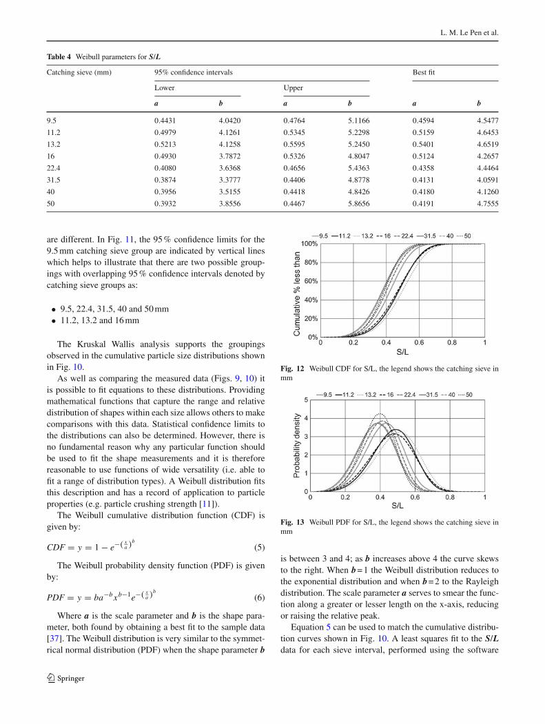
Fig. 12 Weibull CDF for S/L, the legend shows the catching sieve inmm

Fig. 13 Weibull PDF for S/L, the legend shows the catching sieve inmm

is between 3 and 4; as b increases above 4 the curve skewsto the right. When b = 1 the Weibull distribution reduces tothe exponential distribution and when b = 2 to the Rayleighdistribution. The scale parameter a serves to smear the func-tion along a greater or lesser length on the x-axis, reducingor raising the relative peak.

Equation 5 can be used to match the cumulative distribu-tion curves shown in Fig. 10. A least squares fit to the S/Ldata for each sieve interval, performed using the software

123

Dependence of shape on particle size

Table 5 Summary statistics for ellipseness data

Measure Catching sieve (mm)

9.5 11.2 13.2 16 22.4 31.5 40 50

Maximum 0.980 0.983 0.979 0.967 0.976 0.960 0.955 0.959

Upper quartile 0.955 0.959 0.958 0.948 0.755 0.945 0.754 0.942

Mean 0.940 0.940 0.941 0.931 0.929 0.928 0.923 0.925

Lower quartile 0.928 0.924 0.929 0.919 0.913 0.916 0.913 0.914

Minimum 0.860 0.885 0.858 0.836 0.855 0.882 0.854 0.854

SD 0.022 0.023 0.023 0.023 0.025 0.020 0.020 0.022

Fig. 14 Cumulative distributions, Ellipseness, the legend shows thecatching sieve in mm

Fig. 15 Kruskal Wallis evaluation of ellipseness

Matlab [38], gave the values shown in Table 4 for the para-meters a and b. Figure 12 shows the Weibull fits for the CDFsfor the S/L data from each catching sieve size. Comparisonof Fig. 12 with Fig. 10 shows that the Weibull functionsare generally close to the measured data. Figure 13 showsthe Weibull fit for the PDF for the S/L data for each catch-ing sieve size which again shows the differences between the

catching sieve groupings. The data shows that there is a weaktrend for S/L to reduce for larger particles (as found by [6]),but there are exceptions. Some of the data are more spreadout, indicated by a greater standard deviation (Table 3) and orflatter looking PDF (Fig. 13) such as the data in the catchingsieve intervals 11.2, 13.2 and 16 mm. These observations arenot necessarily common to the other form indicators (I/L andS/I) which can be seen by comparing the values in Table 3.

5.2 Roundness

For the dataset shown in Table 2, Image Pro Plus was used toestimate L (Dmax), the perimeter Po and the area Ao of eachparticle, from which the ellipseness was calculated usingEquations 7, 8 and 9. Basic statistics for the ellipseness datais shown in Table 5. Figure 14 shows the cumulative distrib-utions of ellipseness for each sieve interval; as with form, thecurves cover a range of ellipseness values. Figure 15 presentsa Kruskal Wallis analysis of ellipseness. Vertical lines areshown at the 95 % confidence limits for the 22.4 mm data set.Four possible groupings with overlapping 95 % confidenceintervals are apparent denoted by catching sieve groups as:

• 9.5, 11.2, 13.2 mm• 16, 22.4, 31.5, 50 mm• 22.4, 31.5, 40, 50 mm• 11.2, 22.4 mm (just)

These groupings are different from those identified forform.

Again applying a Weibull fit gives the values of parametersa and b shown in Table 6.

Figure 16 shows the CDF calculated using the Weibullfunctions for ellipesness. Figure 17 shows the Weibull PDFswhich are severely skewed by the high shape factor (b).

The ellipseness analysis again demonstrates measurabledifferences in roundness between particles within each sieverange. The data in general suggests that there is a tendencyfor larger size particles to be more angular—again, consistentwith [6]. However, it is still possible for comparisons between

123

L. M. Le Pen et al.

Table 6 Weibull parameters for ellipseness

Catching sieve (mm) 95 % confidence limits Best fit

Lower Upper

a b a b a b

9.5 0.9473 47.3840 0.9531 60.4145 0.9502 53.504

11.2 0.9477 43.9051 0.9540 56.1763 0.9509 49.6631

13.2 0.9484 46.0117 0.9544 58.8745 0.9514 52.0473

16 0.9382 46.1520 0.9441 59.2014 0.9411 52.2711

22.4 0.9342 37.0975 0.9462 56.9157 0.9402 45.9503

31.5 0.9329 43.7752 0.9422 64.0007 0.9375 52.9305

40 0.9281 48.0098 0.9355 67.1111 0.9318 56.7626

50 0.9293 45.4772 0.9391 71.6689 0.9342 57.0903

Fig. 16 Weibull CDFs for ellipseness, the legend shows the catchingsieve in mm

Fig. 17 Weibull PDF for ellipseness, the legend shows the catchingsieve in mm

particular sieve intervals to counter this trend. The actualand idealized distributions of particle aspect ratio S/L andellipseness (angularity) could be used as checks to aid in thecreation of numerical specimens for particle level discreteelement analysis, for example using the approach proposedby Houlsby [39] and developed by Harkness [7] or othercodes capable of generating arbitrary shapes such as Radjaïand Dubois [40].

6 Conclusions

It has been demonstrated that the SEES approach to deter-mining S, I and L is reasonably consistent with a two-viewapproach for the ballast investigated and has the advantageof being less time consuming.

A new measure of roundness (termed ellipseness) has beenintroduced. This relates the perimeter of the particle to theperimeter of an idealized elliptical particle of the same area,and can be determined automatically using appropriate imag-ing and analysis software.

The data indicate a weak trend in the ballast investigatedfor larger particles to have a lower S/L and greater angularity,although comparison between any two individual sieve inter-vals may not follow these trends. However, the ranges of vari-ation in S/L and angularity are relatively small in magnitude,and do not necessarily rule out the use of scaled materials asappropriate substitutes for testing purposes.

Further work is needed to evaluate whether the smallchanges in shape measured in this research translate into dif-ferences in macromechanical behavior that are attributableto shape alone. Such further work might involve the use ofparticle scale discrete element analysis, in which case thedistribution functions presented in this paper could be usedas checks to aid in the creation of numerical specimens.

Acknowledgments This research was facilitated by a grant from theEngineering and Physical Sciences Research Council for the projecttitled “Development and role of structure in railway ballast” (Refer-ence: EP/F062591/1). We also acknowledge the work of Ben Powrie incarrying out particle imaging and Andrew Cresswell for his contribu-tions to the original research proposal.

References

1. Indraratna, B., Ionescu, D., Christie, H.: Shear behavior of railwayballast based on large-scale triaxial tests. J. Geotech. Geoenviron.Eng. 124, 439–450 (1998)

123

Dependence of shape on particle size

2. Anderson, W., Fair, P.: Behavior of railroad ballast under monotonicand cyclic loading. J. Geotech. Geoenviron. Eng. 134, 316 (2008)

3. Aursudkij, B., McDowell, G.R., Collop, A.C.: Cyclic loading ofrailway ballast under triaxial conditions and in a railway test facil-ity. Granul. Matter 11, 391–401 (2009)

4. Cho, G.-C., Dodds, J., Santamarina, J.C.: Particle shape effects onpacking density, stiffness and strength: natural and crushed sands.J. Geotech. Geoenviron. Eng. ASCE 132, 591–602 (2006)

5. Marachi, N.D., Chan, C.K., Seed, H.B.: Evaluation of propertiesof rockfill materials. J. Soil Mech. Found. Div. Proc. Am. Soc. Civ.Eng. 98, 95–114 (1972)

6. Sevi, A.F.: Physical Modeling of Railroad Ballast Using the ParallelGradation Scaling Technique Within the Cyclical Triaxial Frame-work. Doctor of Philosophy Ph.D. thesis, Missouri University ofScience and Technology (2008)

7. Harkness, J.: Potential particles for the modelling of interlockingmedia in three dimensions. Int. J. Numer. Methods Eng. 80, 1573–1594 (2009)

8. Zeller, J., Wullimann, R.: The shear strength of the shell materialsfor the Go-Schenenalp Dam, Switzerland. In: Proceedings of the4th Institutional Journal on SMFE London, pp. 399–404 (1957)

9. Lowe, J.: Shear strength of coarse embankment dam materials. In:Proceedings, 8th Congress on Large dams, pp. 745–761 (1964)

10. Varadarajan, A., Sharma, K.G., Venkatachalam, K., Gupta, A.K.:Testing and modeling two rockfill materials. J. Geotech. Geoenvi-ron. Eng. ASCE 129, 203–218 (2003)

11. McDowell, G.R.: Statistics of soil particle strength. Geotechnique51, 90 (2001)

12. Frossard, E., Hu, E., Dano, C., Hicher, P.-Y.: Rockfill shear strengthevaluation: a rational method based on size effects. Geotechnique62, 415–427 (2012)

13. Hertz, H.R.: Miscellaneous Papers. London MacMillan and Co Ltd,MacMillan and Co, New York (1896)

14. Johnson, K.L.: Contact Mechanics. Cambridge University Press,Cambridge (1985)

15. Cavarretta, I., Coop, M., O’sullivan, C.: The influence of particlecharacteristics on the behaviour of coarse grained soils. Geotech-nique 60, 413–423 (2010)

16. Abbireddy, C.: Particle Form and Its Impact on Packing and ShearBehaviour of Particulate Materials. Doctor of Philosophy, Univer-sity of Southampton (2008)

17. Barrett, P.J.: The shape of rock particles, a critical review. Sedi-mentology 27, 291–303 (1980)

18. Wadell, H.: Volume, shape and roundness of rock particles. J. Geol.40, 443–451 (1932)

19. Francus, P. (ed.): Image Analysis, Sediments and Paleoenviron-ments, vol. 7. Springer, The Netherlands (2004)

20. Erdogan, S.T., Quiroga, P.N., Fowler, D.W., Saleh, H.A., Liv-ingston, R.A., Garboczi, E.J., Ketcham, P.M., Hagedorn, J.G., Sat-terfield, S.G.: Three-dimensional shape analysis of coarse aggre-gates: new techniques for and preliminary results on several differ-ent coarse aggregates and reference rocks. Cem. Concr. Res. 36,1619–1627 (2006)

21. Masad, E., Saadeh, S., Al-Rousan, T., Garboczi, E., Little, D.: Com-putations of particle surface characteristics using optical and X-rayCT images. Comput. Mater. Sci. 34, 406–424 (2005)

22. Taylor, M.A., Garboczi, E.J., Erdogan, S.T., Fowler, D.W.: Someproperties of irregular 3-D particles. Powder Technol. 162, 1–15(2006)

23. Quiroga, P.N., Fowler, D.W.: The Effects of Aggregates Char-acteristics on the Performance of Portland Cement Concrete,Research Report ICAR: 104–1F. International Center for Aggre-gate Research, ICAR (2004)

24. Zingg, T.: Contribution to the gravel analysis (Beitrag zur Schot-teranalyse). Schweiz. Petrog. Mitt. 15(38–140) (1935)

25. Blott, S.J., Pye, K.: Particle shape: a review and new methodsof characterization and classification. Sedimentology 55, 31–63(2008)

26. Sneed, E.D., Folk, R.L.: Pebbles in the lower Colorado River,Texas, a study in particle morphogenesis. J. Geol. 66, 114–150(1958)

27. Pirard, E.: Image measurements. In: Francus, P. (ed.) Image Analy-sis, Sediments and Paleoenvironments. Kluwer Academic Publish-ers, Dordrecht (2005)

28. Abbireddy, C.O.R., Clayton, C.R.I., Schiebel, R.: A method ofestimating the form of coarse particulates. Geotechnique 59(6),493–501 (2009)

29. Garboczi, E.J.: Three-dimensional mathematical analysis of parti-cle shape using X-ray tomography and spherical harmonics: appli-cation to aggregates used in concrete. Cem. Concr. Res. 32(10),1621–1638 (2002)

30. Krumbein, W.C.: Measurement and geological significance ofshape and roundness of sedimentary particles. J. Sedim. Petrol.11, 64–72 (1941)

31. Krumbein, W.C., Sloss, L.L.: Stratigraphy and Sedimentation. W.H. Freeman and Company, San Francisco (1963)

32. Pirard, E.: Shape processing and analysis using the calypter.J. Microsc. 175(3), 214–221 (1994)

33. Mediacy (2011) Image Pro Plus webpage: http://www.mediacy.com/index.aspx?page=IPP Accessed March 2011

34. Ramanujan, S.: Modular equations and approximations to π . Q. J.Pure Appl. Math. 45, 350–372 (1913–1914)

35. Almkvist, G., Berndt, B.: Gauss, Landen, Ramanujan, the arith-meticgeometric mean, ellipses, and the Ladies Diary. Am. Math.Mon. 95, 585–608 (1988)

36. Corder, G. W., Foreman, D. I.: Nonparametric Statistics for Non-statisticians, 1st edn. Wiley, Hoboken (2009)

37. Weibull, W.: A statistical distribution function of wide applicability.J. Appl. Mech. 18, 293–297 (1951)

38. Mathworks: Matlab [Online]. Available: http://www.mathworks.co.uk/products/matlab/ (2012). Accessed May 2012

39. Houlsby, G.T.: Potential particles: a method for modelling non-circular particles in DEM. Comput. Geotech. 36(6), 953–959(2009)

40. Radjaï, F., Dubois, F. (eds.): Discrete Numerical Modeling of Gran-ular Materials: Hardcover, Wiley-Iste, ISBN 978-1-84821-260-2(2011)

123