SANDIA REPORT

SAND2017-8569Unlimited ReleasePrinted August 2017

DAGSENS: Directed Acyclic GraphBased Direct and Adjoint TransientSensitivity Analysis for Event-DrivenObjective Functions

Karthik V. Aadithya, Eric Keiter, and Ting Mei

Prepared by

Sandia National Laboratories

Albuquerque, New Mexico 87185 and Livermore, California 94550

Sandia National Laboratories is a multimission laboratory managed and operated by National Technology and

Engineering Solutions of Sandia, LLC., a wholly owned subsidiary of Honeywell International, Inc., for the

U.S. Department of Energy’s National Nuclear Security Administration under contract DE-NA0003525.

Approved for public release; further dissemination unlimited.

Issued by Sandia National Laboratories, operated for the United States Department of Energy

by National Technology and Engineering Solutions of Sandia, LLC.

NOTICE: This report was prepared as an account of work sponsored by an agency of the United

States Government. Neither the United States Government, nor any agency thereof, nor any

of their employees, nor any of their contractors, subcontractors, or their employees, make any

warranty, express or implied, or assume any legal liability or responsibility for the accuracy,

completeness, or usefulness of any information, apparatus, product, or process disclosed, or rep-

resent that its use would not infringe privately owned rights. Reference herein to any specific

commercial product, process, or service by trade name, trademark, manufacturer, or otherwise,

does not necessarily constitute or imply its endorsement, recommendation, or favoring by the

United States Government, any agency thereof, or any of their contractors or subcontractors.

The views and opinions expressed herein do not necessarily state or reflect those of the United

States Government, any agency thereof, or any of their contractors.

Printed in the United States of America. This report has been reproduced directly from the best

available copy.

Available to DOE and DOE contractors fromU.S. Department of Energy

Office of Scientific and Technical Information

P.O. Box 62

Oak Ridge, TN 37831

Telephone: (865) 576-8401

Facsimile: (865) 576-5728

E-Mail: reports@adonis.osti.gov

Online ordering: http://www.osti.gov/bridge

Available to the public fromU.S. Department of Commerce

National Technical Information Service

5285 Port Royal Rd

Springfield, VA 22161

Telephone: (800) 553-6847

Facsimile: (703) 605-6900

E-Mail: orders@ntis.fedworld.gov

Online ordering: http://www.ntis.gov/help/ordermethods.asp?loc=7-4-0#online

DEP

ARTMENT OF ENERGY

• • UN

ITED

STATES OF AM

ERI C

A

2

SAND2017-8569

Unlimited Release

Printed August 2017

DAGSENS: Directed Acyclic Graph Based Direct and Adjoint

Transient Sensitivity Analysis for Event-Driven Objective

Functions

Karthik V. Aadithya‡, Eric Keiter, and Ting MeiElectrical Models and Simulation

Sandia National LaboratoriesP.O. Box 5800

Albuquerque, NM 87185-1177‡Corresponding author. Email: kvaadit@sandia.gov

3

Abstract

We present DAGSENS, a new theory for parametric transient sensitivity analysis of Differential Al-

gebraic Equation systems (DAEs), such as SPICE-level circuits. The key ideas behind DAGSENS

are, (1) to represent the entire sequence of computations, starting from DAE parameters, all the

way up to the objective function whose sensitivity is needed, as a Directed Acyclic Graph (DAG)

called the “sensitivity DAG”, and (2) to compute the required sensitivites efficiently (with time com-

plexity linear in the size of the sensitivity DAG) by leveraging dynamic programming techniques

to traverse the DAG. DAGSENS is simple, elegant, and easy-to-understand compared to existing

sensitivity analysis approaches; for example, in DAGSENS, one can switch between direct and ad-

joint transient sensitivities just by changing the direction of DAG traversal (i.e., topological order vs.

reverse topological order). Also, DAGSENS is significantly more powerful than existing sensitivity

analysis approaches because it allows one to compute the sensitivities of a much more general

class of objective functions, including those defined based on “events” that occur during a transient

simulation (e.g., a node voltage crossing a particular threshold, a phase-locked loop (PLL) achiev-

ing lock, a signal reaching its maximum/minimum value during a transient run, etc.). In this paper,

we apply DAGSENS to compute the sensitivities of important event-driven performance metrics

in several real-world electronic and biological applications, including high-speed communication

(featuring sub-systems such as I/O links and PLLs), statistical cell library characterization, and

gene expression in Drosophila embryos.

4

Contents

1. Introduction 9

2. Core Techniques and Algorithms for DAG-based Event-driven Sensitivity Analysis 12

2.1 DAE models of dynamical systems . . . . . . . . . . . . . . . . . . . . . . . . . . . . . . . . . . . . . . . . 12

2.2 Transient analysis of DAEs . . . . . . . . . . . . . . . . . . . . . . . . . . . . . . . . . . . . . . . . . . . . . . . 12

2.3 Transient sensitivity analysis of DAEs . . . . . . . . . . . . . . . . . . . . . . . . . . . . . . . . . . . . . . 13

2.4 The sensitivity DAG . . . . . . . . . . . . . . . . . . . . . . . . . . . . . . . . . . . . . . . . . . . . . . . . . . . . . . 14

2.5 Objective functions and the sensitivity DAG . . . . . . . . . . . . . . . . . . . . . . . . . . . . . . . . . 16

2.6 Sensitivity analysis = DAG path enumeration . . . . . . . . . . . . . . . . . . . . . . . . . . . . . . . . 18

2.7 Direct and Adjoint approaches to DAG path enumeration . . . . . . . . . . . . . . . . . . . . . . 19

2.8 Event-driven objective functions . . . . . . . . . . . . . . . . . . . . . . . . . . . . . . . . . . . . . . . . . . . 22

2.9 Sensitivity analysis of event-driven objective functions . . . . . . . . . . . . . . . . . . . . . . . . . 22

2.10 Augmenting the sensitivity DAG for event-driven objective functions . . . . . . . . . . . . . . 23

2.11 DAGSENS: The overall flow for event-driven objective functions . . . . . . . . . . . . . . . . . 25

3. Results 26

3.1 High-speed communication sub-systems . . . . . . . . . . . . . . . . . . . . . . . . . . . . . . . . . . . 26

3.1.1 A “maximum crosstalk” example . . . . . . . . . . . . . . . . . . . . . . . . . . . . . . . . . . . . . 26

3.1.2 A PLL example . . . . . . . . . . . . . . . . . . . . . . . . . . . . . . . . . . . . . . . . . . . . . . . . . . . 28

3.2 Statistical cell library characterization . . . . . . . . . . . . . . . . . . . . . . . . . . . . . . . . . . . . . . 30

3.3 Biological applications . . . . . . . . . . . . . . . . . . . . . . . . . . . . . . . . . . . . . . . . . . . . . . . . . . . . 31

5

4. Summary, Conclusions, and Future Work 36

6

List of Figures

2.1 The DAG structure underlying a transient simulation. . . . . . . . . . . . . . . . . . . . . . . . . . 15

2.2 Adding a final point objective function to the sensitivity DAG. . . . . . . . . . . . . . . . . . . . . 17

2.3 Adding an integral objective function to the sensitivity DAG. . . . . . . . . . . . . . . . . . . . . . 17

2.4 The DAG of Fig. 2.2, with edge-weights denoted by partial derivatives. . . . . . . . . . . . 18

2.5 The key ideas behind efficient direct and adjoint DAG path enumeration in DAGSENS. 20

2.6 Adding (a) events, and (b) an event-driven objective, to the sensitivity DAG. . . . . . . . . 24

3.1 (a) The circuit used to determine the magnitude of crosstalk induced by an aggres-

sor on a victim. (b, c) Transient simulation of the circuit in (a) without and with

pre/de-emphasis respectively, with the event corresponding to maximum crosstalk

in each case. (d through i) Sensitivities of the maximum crosstalk with respect to

each segment resistance (d, e), segment capacitance (f, g), and coupling capaci-

tance (h, i), without (d, f, h) and with (e, g, i) pre/de-emphasis. . . . . . . . . . . . . . . . . . . 27

3.2 (a) Block diagram of a PLL, with the underlying equations, (b, c) Transient simula-

tion of low-bandwidth (b) and high-bandwidth (c) PLLs on an input waveform that

abruptly changes frequency at t = 50ns. The high-bandwidth PLL regains lock more

quickly, but features a larger peak-to-peak swing in Vctl around its ideal DC value. . 29

3.3 A CMOS NAND gate driving an RC load. . . . . . . . . . . . . . . . . . . . . . . . . . . . . . . . . . . . 30

3.4 Transient simulation of the CMOS NAND gate of Fig. 3.3 for two different input

transitions, showing the 20% and 80% “transition complete” events, and the corre-

sponding “gate delay” objective function in each case. . . . . . . . . . . . . . . . . . . . . . . . . . 31

3.5 A model for gene expression in a Drosophila embryo, featuring transcription, trans-

lation, and decay (part a), as well as diffusion across nuclei (part b). . . . . . . . . . . . . . 32

3.6 Transient simulation of gene expression in a Drosophila embryo. . . . . . . . . . . . . . . . . 33

3.7 Sensitivities of peak mRNA and protein concentrations, as well as the times at which

these peak concentrations occur, across nuclei, for the Drosophila embryo gene

expression system. . . . . . . . . . . . . . . . . . . . . . . . . . . . . . . . . . . . . . . . . . . . . . . . . . . . . . . 34

7

8

1. Introduction

This report is about a new, elegant, and powerful approach to computing transient sensitivities of

dynamical systems. Such sensitivities have several well-known uses in scientific and engineering

applications, including design optimization [1], uncertainty quantification [2], stability analysis [3],

and transient global error control [4].

Parametric transient sensitivities have long been used in integrated circuit design [5, 6]. To this

day, such sensitivities are being heavily used for a variety of circuit design applications, including

optimization and tuning [7], yield estimation [8], performance modelling [9], statistical cell library

characterization [10], etc. Indeed, as CMOS technology moves to progressively smaller feature

sizes (7 nm and below), and with the advent of near-threshold and sub-threshold computing, the

importance of parametric sensitivity analysis in variability-aware circuit design is likely to grow

even further, due to the increasingly significant role played by parameter variability in determining

circuit performance (speed, power consumption, bandwidth, etc.), as well as yield [8–10].

Parametric sensitivities are also important for analyzing and designing biological systems. Appli-

cations in this domain include identifying influential kinetic parameters and model order reduction

of chemical reaction networks [11], improving model accuracy and separating biological mecha-

nisms from mathematical artifacts [12,13], calculating the relative importance of different parallelly

executing processes in biological phenomena such as gene expression [14], understanding the

factors at work behind the robustness of biological systems to parameter variability [15,16], etc.

Broadly speaking, there are two main approaches to sensitivity analysis: “direct” and “adjoint”.

Direct methods [6] involve computing the sensitivities of all intermediate quantities with respect

to system parameters (by repeatedly applying the chain rule of differentiation), until the sensitivity

of the desired “objective function” is eventually found. Thus, direct methods are relatively easy

to understand and implement, but scale poorly for problems with large numbers of parameters.

Adjoint methods [3,10,17–20], on the other hand, work backwards; they compute the sensitivities

of the objective function with respect to all intermediate quantities, until the desired sensitivity of

the objective function with respect to the parameters is eventually found. Thus, adjoint methods

are somewhat harder to understand and implement, but unlike direct methods, they scale well to

problems with large numbers of parameters, as long as the dimensions of the objective functions

are relatively small. In other words, if one is only interested in calculating the sensitivities of a

small number of performance metrics with respect to a large number of parameters, then adjoint

methods allow one to take advantage of the small dimensionality of the performance space to sig-

nificantly speed up sensitivity analysis. Modern circuit simulation problems often fit this description;

in these cases, computing sensitivities is usually practical only using adjoint methods.

Despite their long history and continued importance, we believe that adjoint methods are not well

9

understood. This, we believe, is at least in part because existing descriptions in the literature

use hard-to-understand concepts and somewhat esoteric constructs such as adjoint circuits [5,7],

integrating Differential-Algebraic Equations (DAEs) backwards in time [17, 18, 20], complicated

mathematics involving feeding δ-function inputs to DAEs [17], etc.

Moreover, previous works on sensitivity analysis have lacked generality with respect to the ob-

jective functions supported. Indeed, they have restricted themselves to the sensitivities of DAE

solution variables at specific points in time (i.e., “final point” objective functions, §2.5) [10, 19], or

integrals of the solution over time (i.e., “integral” objective functions, §2.5) [18,20], or simple combi-

nations thereof, such as the ratio of two integrals [17]. In practice, such simple objective functions

are often inadequate because real-world objectives of interest often do not fit either a “final point”

or an “integral” description. Circuit designers frequently need more advanced metrics, which we

describe as “event-driven” objectives. Such objectives are defined based on “events” that take

place during the course of a transient run. Examples include a signal crossing a user-specified

threshold, or possibly reaching a maximum/minimum value. A more complicated objective function

could be the amount of time taken by a phase-locked loop (PLL) to lock to a new input frequency.

The “achievement of lock” by a PLL is a transient event, and so the “time to lock” is an event-driven

objective function, whose sensitivities with respect to PLL parameters are of interest to designers.

These types of “event-driven” objectives are common in circuit analysis, but are outside the scope

of existing sensitivity analysis tools. Indeed, many popular circuit simulators already provide ways

to calculate such event-driven objectives (e.g., the .MEASURE feature found in HSPICE R© [21] and

Xyce R© [22]); we believe we are the first to address the problem of calculating the sensitivities of

such objectives.

In this report, we develop DAGSENS, a new theory for transient sensitivity analysis based on

Directed Acyclic Graphs (DAGs). In this approach, we construct a DAG where each intermedi-

ate quantity computed during a transient run is represented as a node, starting from the DAE

parameters, all the way up to the objective function (§2.4, §2.5). Once this DAG is constructed,

all required sensitivities can be obtained by traversing it, using efficient techniques based on dy-

namic programming (§2.7) [23, 24]. A key advantage is the simplicity and elegance of the DAG

approach, which we believe previous approaches lack; for example, in DAGSENS, to switch from

direct to adjoint sensitivity analysis, one simply changes the direction of DAG traversal from topo-

logical order to reverse topological order (§2.7), much like forward and reverse mode automatic

differentiation [25,26]. Moreover, DAGSENS works seamlessly for all integration methods, without

the need for adjoint circuits, or complicated backwards-in-time integration formulas, or δ-function

inputs to DAEs, etc. We believe that, due to its ease of understandability, DAGSENS can make

the benefits of sensitivity analysis accessible to a wider audience, including device engineers, cir-

cuit designers, and students. Also, DAGSENS is more powerful than existing sensitivity analysis

approaches, because it is capable of handling more general objective functions. For example, we

define and develop the notion of event-driven objectives described above, and show how to use

DAGSENS to compute direct and adjoint transient sensitivities for such objective functions (§2.8

through §2.11).

The rest of this report is organized as follows. In Chapter 2, we provide some technical back-

ground (on DAEs, transient analysis, transient sensitivity analysis, etc.), and then delve into the

key ideas and core concepts underlying DAGSENS. In Chapter 3, we apply DAGSENS to compute

event-driven sensitivities in several representative real-world electronic and biological applications,

including high-speed communication (§3.1), statistical cell library characterization (§3.2), and gene

10

expression in Drosophila embryos (§3.3). In Chapter 4, we conclude and provide directions for fu-

ture work that we intend to pursue.

11

2. Core Techniques and

Algorithms for DAG-based

Event-driven Sensitivity

Analysis

2.1 DAE models of dynamical systems

Throughout this report, we assume that the system we wish to analyze is a DAE of the form:

d

dt~q(~x(t), ~p ) + ~f(~x(t), ~u(t), ~p ) = 0, (2.1)

where ~x is the system’s state vector (e.g., a list of voltages and currents), ~p is a vector of parame-

ters with respect to which we wish to compute sensitivities (transistor widths and lengths, parasitic

resistances and capacitances, etc.), ~u is a vector of inputs to the system, and t denotes time. We

note that Eq. (2.1) is capable of modelling virtually any electronic circuit at the SPICE level, and

many biological systems as well [27–29].

2.2 Transient analysis of DAEs

Given an initial condition ~x(t0) = ~x0, and time-varying inputs ~u(t) to the DAE of Eq. (2.1), transient

analysis refers to the problem of solving for the time-varying DAE state ~x(t) over a time-interval

[t0, tf ]. This is accomplished by discretizing time into a sequence t0, t1, . . . , tN−1 (where

tN−1 = tf ), and then approximating the respective DAE states ~x0, ~x1, . . . , ~xN−1 by solving a

sequence of “Linear Multi-Step” (LMS) equations of the form [27,28,30,31]:

mi∑

j=0

(

αi(−j) ~q (~xi−j, ~p ) + βi(−j) ~f (~xi−j, ~u(ti−j), ~p ))

= ~0. (2.2)

Thus, at each step i (where 1 ≤ i ≤ N − 1), one solves Eq. (2.2) (using techniques like Newton-

Raphson iteration, homotopy, etc.) to determine ~xi, based on mi previously calculated ~x values

(from earlier steps). Table 2.1 lists the α and β coefficients used in Eq. (2.2) by several common

12

Method mi Coefficient j = 2 j = 1 j = 0

FE 1αi(−j) – − 1

ti−ti−1

1ti−ti−1

βi(−j) – 1 0

BE 1αi(−j) – − 1

ti−ti−1

1ti−ti−1

βi(−j) – 0 1

TRAP 1αi(−j) – − 1

ti−ti−1

1ti−ti−1

βi(−j) – 0.5 0.5

GEAR2 2αi(−j)

1ti−1−ti−2

− 1ti−ti−2

− 1ti−ti−1

− 1ti−1−ti−2

1ti−ti−1

+ 1ti−ti−2

βi(−j) 0 0 1

Table 2.1. Coefficients used in Eq. (2.2) by several common LMS

methods.

LMS methods, including Forward Euler (FE), Backward Euler (BE), Trapezoidal (TRAP), and second-

order Gear (GEAR2) [27,30,32,33].

2.3 Transient sensitivity analysis of DAEs

Suppose we have a DAE in the form of Eq. (2.1), with nominal parameters ~p ⋆, and transient

solution ~x⋆(t) over the interval [t0, tf ] (using the convention that starred quantities denote nominal

values, i.e., those evaluated at ~p ⋆). The question behind transient sensitivity analysis is: if we

perturb the parameters slightly, how will the transient solution change? More precisely, suppose

we change the parameters from ~p ⋆ to ~p ⋆ + ∆~p, and as a result, the transient solution changes

from ~x⋆(t) to ~x⋆(t)+∆~x(t). The question is: what is the relationship between ∆~x(t) and ∆~p, in the

limit as ∆~p → ~0? The answer is obtained by doing a perturbation analysis of Eq. (2.1) [17–19]:

∆~x(t) = Sx(t)∆~p, where (2.3)[d

dt

(J⋆qx(t)Sx(t) + J⋆

qp(t))]

+[J⋆fx(t)Sx(t) + J⋆

fp(t)]= 0|~x⋆|×|~p⋆|. (2.4)

The J terms in Eq. (2.4) denote nominal time-varying Jacobians, i.e.,

J⋆qx(t) ,

∂~q

∂~x

∣∣∣∣~x⋆(t), ~p⋆

, J⋆qp(t) ,

∂~q

∂~p

∣∣∣∣~x⋆(t), ~p⋆

,

13

J⋆fx(t) ,

∂ ~f

∂~x

∣∣∣∣∣~x⋆(t), ~u(t), ~p⋆

, and J⋆fp(t) ,

∂ ~f

∂~p

∣∣∣∣∣~x⋆(t), ~u(t), ~p⋆

. (2.5)

Since ∆~x(t) is obtained by multiplying Sx(t) with ∆~p (Eq. 2.3), Sx(t) is called the sensitivity of ~x(t)with respect to ~p, evaluated at ~p ⋆. And Eq. (2.4), a matrix-valued DAE that tracks the evolution of

the |~x⋆| × |~p ⋆| matrix Sx(t) over time, is called the “sensitivity DAE”.

Note that the sensitivity DAE does not directly give us Sx(t). Rather, it needs to be solved for

Sx(t) [6]. The “direct” approach for this involves two rounds of transient analysis (although, in

practice, they are combined into one to save memory). In the first round, the original DAE (Eq. 2.1)

is solved using LMS techniques (§2.2). This yields a sequence of time-points ti (where 0 ≤ i ≤N − 1 and tN−1 = tf ), as well as a corresponding sequence of DAE states ~x ⋆(i) (§2.2). These,

in turn, are used to compute Jacobian sequences: J⋆qx(i), J⋆

qp(i), J⋆fx(i), and J⋆

fp(i).

In the second round, the sensitivity DAE (Eq. 2.4) is solved using the same LMS techniques, and

the same sequence of LMS methods (FE, BE, etc.) used for the first round. The LMS equations

that are solved (similar to Eq. 2.2) are:

mi∑

j=0

[

αi(−j)[J⋆qx(i− j)Sx(i− j) + J⋆

qp(i− j)]

+ βi(−j)[J⋆fx(i− j)Sx(i− j) + J⋆

fp(i− j)]]

= 0|~x⋆|×|~p⋆|, (2.6)

where the α and β coefficients, as before, are found in Table 2.1. Solving the equations above

yields the required sensitivities Sx(i), for 0 ≤ i ≤ N , discretized over [t0, tf ]. Note that the initial

condition Sx(0) (i.e., the sensitivity of the initial DAE state ~x⋆(0)) is needed to start the chain of

solves above; this is usually found by DC (steady-state) sensitivity analysis [27].

2.4 The sensitivity DAG

Each step of the transient analysis of §2.2 builds on previously computed DAE states, to solve for a

new DAE state. This sequence of computations fits naturally into a DAG structure (Fig. 2.1), much

like DAGs used in automatic differentiation [26], or Boolean function representation [34].

The nodes of the “sensitivity DAG” in Fig. 2.1 represent the quantities that are computed during

the transient simulation, and are labelled as such. The edges represent dependencies amongst

these quantities. For example, Fig. 2.1 assumes that the initial condition ~x⋆(0) is computed from ~p ⋆

(e.g., via DC analysis [27, 28]); so, there is an edge from the ~p ⋆ node to the ~x⋆(0) node. Similarly,

~x⋆(1) is assumed to be computed from ~x⋆(0) and ~p ⋆ by solving Eq. (2.2), using an LMS method

with memory m1 = 1, such as FE, BE, or TRAP (Table 2.1). So, there are edges leading from both

~p ⋆ and ~x⋆(0) to ~x⋆(1). Finally, ~x⋆(2) is assumed to be computed via an LMS method like GEAR2

that has memory m2 = 2 (Table 2.1). Therefore, when Eq. (2.2) is solved to determine ~x⋆(2), both

14

Figure 2.1. The DAG structure underlying a transient simulation.

~x⋆(0) and ~x⋆(1), as well as ~p ⋆, are used in the computation. So, there are edges from all these

three nodes to ~x ⋆(2).

While Fig. 2.1 stops at ~x⋆(2) for lack of space, the ideas behind the DAG construction can be

extended to the entire length of the transient simulation. In general, if the simulation has N points,

with indices 0 ≤ i ≤ N − 1, the corresponding sensitivity DAG will have N + 1 nodes (one for ~p ⋆,

and one for each ~x ⋆(i)). The ~x⋆(0) node will have exactly one incoming edge (from ~p ⋆). For all

other ~x⋆(i), the number of incoming edges will be 1 + mi, where mi is the memory of the LMS

method used to compute ~x⋆(i) via Eq. (2.2). One of these edges will originate at ~p ⋆, while the

others will originate at the mi nodes prior to ~x⋆(i), i.e., the nodes ~x⋆(i− j) for 1 ≤ j ≤ mi.

Also, each edge of the sensitivity DAG has a weight (Fig. 2.1). The weight of an edge from node u

to node v, denoted w(u, v), is equal to the partial derivative (or sensitivity) of v with respect to u; it

measures how much a small perturbation in u will affect the value of v. The weight w(~p ⋆, ~x⋆(0)) is

obtained by doing a DC perturbation analysis of Eq. (2.1) [27], while all other weights are obtained

by doing a perturbation analysis of Eq. (2.2):

w(~p ⋆, ~x⋆(0)) =∂~x⋆(0)

∂~p ⋆ = −J⋆fx(0)

−1J⋆fp(0), (2.7)

w(~p ⋆, ~x⋆(i)) =∂~x ⋆(i)

∂~p ⋆ = −

[

αi(0)J⋆qx(i) + βi(0)J

⋆fx(i)

]−1

mi∑

j=0

(

αi(−j)J⋆qp(i− j) + βi(−j)J⋆

fp(i− j)

)

,

∀ 1 ≤ i ≤ N − 1, and (2.8)

15

w(~x ⋆(i− j), ~x ⋆(i)) =∂~x ⋆(i)

∂~x ⋆(i− j)= −

[

αi(0)J⋆qx(i) + βi(0)J

⋆fx(i)

]−1

[

αi(−j)J⋆qx(i− j) + βi(−j)J⋆

fx(i− j)

]

,

∀ 1 ≤ i ≤ N − 1, 1 ≤ j ≤ mi. (2.9)

2.5 Objective functions and the sensitivity

DAG

In many applications, we are not directly interested in the sensitivities of ~x⋆(t), but would like

to compute the sensitivities of important transient performance metrics (i.e., “objective functions”)

derived from ~x⋆(t) (and denoted ~φ⋆). Below, we discuss two kinds of objective functions commonly

found in the sensitivity analysis literature (“final point” and “integral” objectives), and show how to

add these to the sensitivity DAG.

Final point objectives. These take the form [10,19]:

~φ⋆ = ~h(~x⋆(N − 1), ~p ⋆), (2.10)

where ~x⋆(N − 1) is the final point in the transient simulation. Note that, if ~h(., .) needs to be

evaluated at multiple time-points, then each needs to be considered a separate objective, which

will increase the dimension of the objective function. The sensitivity Sφ of a final point objective

function, evaluated at ~p ⋆, is given by:

Sφ = J⋆hx(N − 1)Sx(N − 1) + J⋆

hp(N − 1), (2.11)

where the Jacobian symbols have their usual meanings.

To add such an objective function to the sensitivity DAG, we add a new node ~φ⋆ with two incoming

edges: one from ~p ⋆ with weight J⋆hp(N − 1), and one from ~x⋆(N − 1) with weight J⋆

hx(N − 1) (as

shown in Fig. 2.2 for N = 3).

Integral objectives. These take the form [18,20]:

~φ⋆ =

∫ tf

t=t0

~h(t, ~x⋆(t), ~p ⋆) dt. (2.12)

Therefore, we have:

16

Figure 2.2. Adding a final point objective function to the sensitiv-ity DAG.

Sφ =

∫ tf

t=t0

(J⋆hx(t)Sx(t) + J⋆

hp(t))dt. (2.13)

In practice, the integral in Eq. (2.13) is approximated by a summation:

Sφ ≈N−2∑

i=0

[(J⋆hx(i)Sx(i) + J⋆

hp(i))(ti+1 − ti)

]. (2.14)

Figure 2.3. Adding an integral objective function to the sensitivity

DAG.

To add such an objective function to the sensitivity DAG, we add a new node ~φ⋆, with N incoming

edges: one from ~p ⋆, and the rest from ~x⋆(i), where 0 ≤ i ≤ N − 2 (i.e., from every point in the

transient simulation except the last, as illustrated in Fig. 2.3 for N = 3). The weights of these

edges are:

17

w(~p ⋆, ~φ⋆) =N−2∑

i=0

(J⋆hp(i)(ti+1 − ti)

), and (2.15)

w(~x ⋆(i), ~φ⋆) = J⋆hx(i)(ti+1 − ti), ∀ 0 ≤ i ≤ N − 2. (2.16)

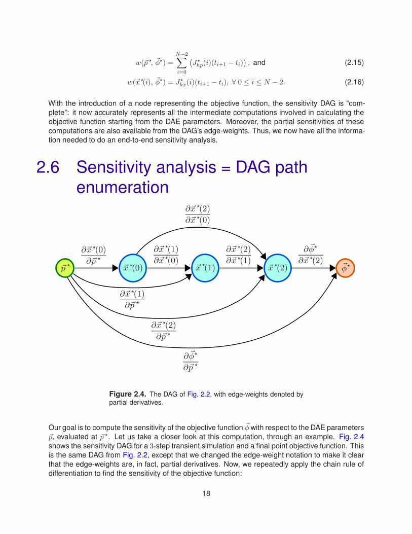
With the introduction of a node representing the objective function, the sensitivity DAG is “com-

plete”: it now accurately represents all the intermediate computations involved in calculating the

objective function starting from the DAE parameters. Moreover, the partial sensitivities of these

computations are also available from the DAG’s edge-weights. Thus, we now have all the informa-

tion needed to do an end-to-end sensitivity analysis.

2.6 Sensitivity analysis = DAG path

enumeration

Figure 2.4. The DAG of Fig. 2.2, with edge-weights denoted by

partial derivatives.

Our goal is to compute the sensitivity of the objective function ~φ with respect to the DAE parameters

~p, evaluated at ~p ⋆. Let us take a closer look at this computation, through an example. Fig. 2.4

shows the sensitivity DAG for a 3-step transient simulation and a final point objective function. This

is the same DAG from Fig. 2.2, except that we changed the edge-weight notation to make it clear

that the edge-weights are, in fact, partial derivatives. Now, we repeatedly apply the chain rule of

differentiation to find the sensitivity of the objective function:

18

Sensitivitywe need

=d~φ

d~p

∣∣∣∣∣~p⋆

=d~φ⋆

d~p ⋆

︸︷︷︸

Chain Rule

=∂~φ⋆

∂~p ⋆ +∂~φ⋆

∂~x⋆(2)

d~x ⋆(2)

d~p ⋆

︸ ︷︷ ︸

Chain Rule

=∂~φ⋆

∂~p ⋆ +∂~φ⋆

∂~x⋆(2)

(∂~x⋆(2)

∂~p ⋆ +∂~x ⋆(2)

∂~x ⋆(1)

d~x⋆(1)

d~p ⋆

︸ ︷︷ ︸

Chain Rule

+∂~x⋆(2)

∂~x⋆(0)

d~x⋆(0)

d~p ⋆

︸ ︷︷ ︸

Chain Rule

)

=∂~φ⋆

∂~p ⋆ +∂~φ⋆

∂~x⋆(2)

(∂~x⋆(2)

∂~p ⋆ +∂~x ⋆(2)

∂~x ⋆(1)

(∂~x ⋆(1)

∂~p ⋆ +∂~x⋆(1)

∂~x⋆(0)

d~x ⋆(0)

d~p ⋆

︸ ︷︷ ︸

Chain Rule

)

+∂~x⋆(2)

∂~x⋆(0)

∂~x⋆(0)

∂~p ⋆

)

=∂~φ⋆

∂~p ⋆ +∂~φ⋆

∂~x⋆(2)

(∂~x⋆(2)

∂~p ⋆ +∂~x ⋆(2)

∂~x ⋆(1)

(∂~x ⋆(1)

∂~p ⋆ +∂~x⋆(1)

∂~x⋆(0)

∂~x⋆(0)

∂~p ⋆

)

+∂~x⋆(2)

∂~x⋆(0)

∂~x⋆(0)

∂~p ⋆

)

=

[∂~φ⋆

∂~p ⋆

︸︷︷︸

Path: ~p⋆→ ~φ⋆

+∂~φ⋆

∂~x ⋆(2)

∂~x⋆(2)

∂~p ⋆

︸ ︷︷ ︸

Path: ~p⋆→ ~x⋆(2)→ ~φ⋆

+∂~φ⋆

∂~x⋆(2)

∂~x⋆(2)

∂~x⋆(1)

∂~x ⋆(1)

∂~p ⋆

︸ ︷︷ ︸

Path: ~p⋆→ ~x⋆(1)→ ~x⋆(2)→ ~φ⋆

+∂~φ⋆

∂~x ⋆(2)

∂~x ⋆(2)

∂~x ⋆(1)

∂~x⋆(1)

∂~x⋆(0)

∂~x⋆(0)

∂~p ⋆

︸ ︷︷ ︸

Path: ~p⋆→ ~x⋆(0)→ ~x⋆(1)→ ~x⋆(2)→ ~φ⋆

+∂~φ⋆

∂~x ⋆(2)

∂~x⋆(2)

∂~x⋆(0)

∂~x⋆(0)

∂~p ⋆

︸ ︷︷ ︸

Path: ~p⋆→ ~x⋆(0)→ ~x⋆(2)→ ~φ⋆

]

=∑

π | π is a path from

~p⋆ to ~φ⋆ in the sensitivity DAG

(

Product of edge-weights of π in reverse

)

.

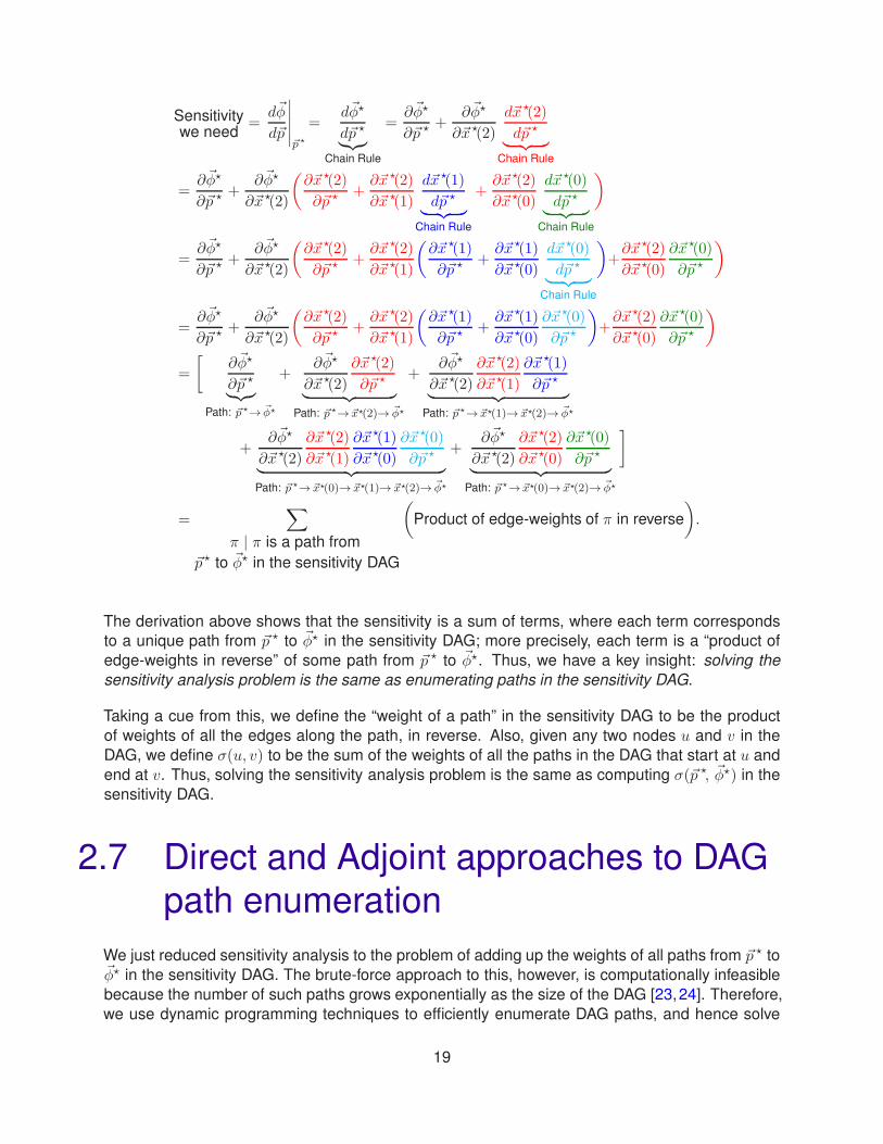
The derivation above shows that the sensitivity is a sum of terms, where each term corresponds

to a unique path from ~p ⋆ to ~φ⋆ in the sensitivity DAG; more precisely, each term is a “product of

edge-weights in reverse” of some path from ~p ⋆ to ~φ⋆. Thus, we have a key insight: solving the

sensitivity analysis problem is the same as enumerating paths in the sensitivity DAG.

Taking a cue from this, we define the “weight of a path” in the sensitivity DAG to be the product

of weights of all the edges along the path, in reverse. Also, given any two nodes u and v in the

DAG, we define σ(u, v) to be the sum of the weights of all the paths in the DAG that start at u and

end at v. Thus, solving the sensitivity analysis problem is the same as computing σ(~p ⋆, ~φ⋆) in the

sensitivity DAG.

2.7 Direct and Adjoint approaches to DAG

path enumeration

We just reduced sensitivity analysis to the problem of adding up the weights of all paths from ~p ⋆ to~φ⋆ in the sensitivity DAG. The brute-force approach to this, however, is computationally infeasible

because the number of such paths grows exponentially as the size of the DAG [23,24]. Therefore,

we use dynamic programming techniques to efficiently enumerate DAG paths, and hence solve

19

the sensitivity analysis problem in linear time in the size of the DAG [23,24].

Direct sensitivity analysis: Optimal sub-structure for dynamic programming

(a)

Adjoint sensitivity analysis: Optimal sub-structure for dynamic programming

(b)

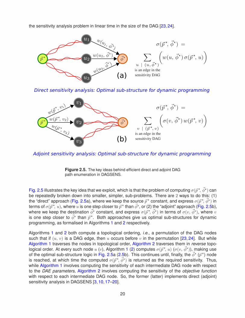
Figure 2.5. The key ideas behind efficient direct and adjoint DAGpath enumeration in DAGSENS.

Fig. 2.5 illustrates the key idea that we exploit, which is that the problem of computing σ(~p ⋆, ~φ⋆) can

be repeatedly broken down into smaller, simpler, sub-problems. There are 2 ways to do this: (1)

the “direct” approach (Fig. 2.5a), where we keep the source ~p ⋆ constant, and express σ(~p ⋆, ~φ⋆) in

terms of σ(~p ⋆, u), where u is one step closer to ~p ⋆ than ~φ⋆, or (2) the “adjoint” approach (Fig. 2.5b),

where we keep the destination ~φ⋆ constant, and express σ(~p ⋆, ~φ⋆) in terms of σ(v, ~φ⋆), where v

is one step closer to ~φ⋆ than ~p ⋆. Both approaches give us optimal sub-structures for dynamic

programming, as formalised in Algorithms 1 and 2 respectively.

Algorithms 1 and 2 both compute a topological ordering, i.e., a permutation of the DAG nodes

such that if (u, v) is a DAG edge, then u occurs before v in the permutation [23, 24]. But while

Algorithm 1 traverses the nodes in topological order, Algorithm 2 traverses them in reverse topo-

logical order. At every such node u (v), Algorithm 1 (2) computes σ(~p ⋆, u) (σ(v, ~φ⋆)), making use

of the optimal sub-structure logic in Fig. 2.5a (2.5b). This continues until, finally, the ~φ⋆ (~p ⋆) node

is reached, at which time the computed σ(~p ⋆, ~φ⋆) is returned as the required sensitivity. Thus,

while Algorithm 1 involves computing the sensitivity of each intermediate DAG node with respect

to the DAE parameters, Algorithm 2 involves computing the sensitivity of the objective function

with respect to each intermediate DAG node. So, the former (latter) implements direct (adjoint)

sensitivity analysis in DAGSENS [3,10,17–20].

20

Algorithm 1: Direct transient sensitivity analysis in DAGSENS

Input: The sensitivity DAG G, with nodes ~p ⋆ and ~φ⋆ representing the DAE parameters and

the objective function respectively

Output: The sensitivity σ(~p ⋆, ~φ⋆), calculated via dynamic programming using the “direct”

optimal sub-structure (Fig. 2.5a)

1 σ(~p ⋆, ~p ⋆) = I|~p⋆|×|~p⋆| // identity matrix

2 order = topological sort(G)3 for u in order do

4 σ(~p ⋆, u) = 0|u|×|~p⋆|

5 for v such that (v, u) is an edge in G do

6 σ(~p ⋆, u) += w(v, u) σ(~p ⋆, v)

7 return σ(~p ⋆, ~φ⋆)

Algorithm 2: Adjoint transient sensitivity analysis in DAGSENS

Input: The sensitivity DAG G, with nodes ~p ⋆ and ~φ⋆ representing the DAE parameters and

the objective function respectively

Output: The sensitivity σ(~p ⋆, ~φ⋆), calculated via dynamic programming using the “adjoint”

optimal sub-structure (Fig. 2.5b)

1 σ(~φ⋆, ~φ⋆) = I|~φ⋆|×|~φ⋆| // identity matrix

2 order = reversed(topological sort(G))3 for v in order do

4 σ(v, ~φ⋆) = 0|~φ⋆|×|v|

5 for u such that (v, u) is an edge in G do

6 σ(v, ~φ⋆) += σ(u, ~φ⋆) w(v, u)

7 return σ(~p ⋆, ~φ⋆)

21

Finally, Line 6 of Algorithm 2 involves pre-multiplying the edge-weightw(v, u) by the matrix σ(u, ~φ⋆).Since most edge-weights are of the form B−1C (Eqs. 2.7, 2.8, and 2.9), this is a computation of the

form AB−1C, which can be done either as A(B−1C), or as (AB−1)C = ((BT )−1AT )TC (where

matrix/matrix solves are sparse in many applications of interest). If the number of rows of A is

much smaller than the number of columns of C (i.e., the dimension of the objective function is

much smaller than that of the DAE parameter space), the latter is likely to be much more efficient

than the former, which we exploit heavily in DAGSENS.

2.8 Event-driven objective functions

As mentioned in Chapter 1, we would like to define “events” that happen during a transient simu-

lation (e.g., a node voltage crossing a particular threshold, a PLL in a circuit achieving lock, etc.),

and then compute sensitivities of objectives that are based on these events. For our purposes, an

“event” ev is specified by the condition:

gev(τ⋆ev, ~x

⋆(τ⋆ev), ~p⋆) = 0, (2.17)

where τ⋆ev is the time at which the event occurs during a transient simulation. In practice, we may

need additional constraints to uniquely identify the event (such as limits on τ⋆ev, or a specification

such as “the third time Eq. (2.17) is satisfied”, etc.). But for sensitivity analysis, we can ignore

these additional specifications because we only do perturbation analysis of Eq. (2.17) in a small

neighbourbood around τ⋆ev. Also, we note that events corresponding to a signal reaching its maxi-

mum/minimum value are specified by adding a new DAE state variable representing the derivative

of the signal in question, and by equating this variable to zero via Eq. (2.17) (see Chapter 3 for

examples).

Given a sequence of M events 1 ≤ ev ≤ M , our event-driven objective function takes the form:

~φ⋆ = ~h(τ⋆1 , τ⋆2 , . . . , τ

⋆M , ~x⋆(τ⋆1 ), ~x

⋆(τ⋆2 ), . . . , ~x⋆(τ⋆M ), ~p ⋆). (2.18)

Thus, event-driven objective functions depend on the times of occurrence of a set of events, as well

as the DAE states at these times, both of which change when the DAE parameters are perturbed.

2.9 Sensitivity analysis of event-driven

objective functions

Let us denote by Sτev and Sxev, where 1 ≤ ev ≤ M , the sensitivities of our event times, and DAE

states at these times, respectively. Note that Sxev 6= Sx(τ⋆ev); while Sx(τ

⋆ev) only takes into account

the sensitivity of the DAE state ~x, Sxev takes into account the sensitivities of both the DAE state ~x

and the event time τev. With this distinction in mind, perturbation analysis of Eq. (2.17) yields:

22

Sτev = −J⋆gevxSx(τ

⋆ev) + J⋆

gevp

J⋆gevx

~x⋆(τ⋆ev) + J⋆

gevτ

, and (2.19)

Sxev = Sx(τ⋆ev) + ~x

⋆(τ⋆ev)Sτev , where (2.20)

~x⋆(τ⋆ev) =

d

dt~x⋆(t)

∣∣∣∣τ⋆ev

, ∀ 1 ≤ ev ≤ M, (2.21)

and where Jacobian terms have their usual meanings, and are all evaluated at (τ⋆ev, ~x⋆(τ⋆ev), ~p

⋆).Therefore, we first need to solve for the event, i.e., find τ⋆ev and ~x⋆(τ⋆ev), before we can compute

Sτev and Sxev. We do this by finding a time-point ti of the transient simulation where the gev(., ., .)function undergoes a sign change between ti and ti+1. We then use a modified LMS strategy to

solve for the event, by solving:

(

αev(0, τ⋆ev) ~q (~x

⋆(τ⋆ev), ~p⋆) + βev(0, τ

⋆ev)

~f (~x⋆(τ⋆ev), ~u(τ⋆ev), ~p

⋆))

+

mev∑

j=1

(

αev(−j, τ⋆ev) ~q (~x⋆(i− j + 1), ~p ⋆)

+ βev(−j, τ⋆ev)~f (~x ⋆(i− j + 1), ~u(ti−j+1), ~p

⋆)

)

= ~0, and (2.22)

gev(τ⋆ev, ~x

⋆(τ⋆ev), ~p⋆) = 0. (2.23)

These equations are similar to Eq. (2.2). But here, we treat both the next time-point τ⋆ev and

the next DAE state ~x⋆(τ⋆ev) as unknowns. So, the α and β coefficients become functions of the

unknowns as well. Also, we use LMS approximations to calculate the ~x⋆(τ⋆ev) term in Eqs. (2.19)

and (2.20).

Finally, the sensitivity of our event-driven objective function is given by:

Sφ = J⋆hp +

M∑

ev=1

(

J⋆hτev

Sτev + J⋆hx(τev)

Sxev

)

. (2.24)

2.10 Augmenting the sensitivity DAG for

event-driven objective functions

Fig. 2.6 shows how to add an event-driven objective function to the sensitivity DAG. For each event

1 ≤ ev ≤ M , we add three new nodes (Fig. 2.6a): a partial ~x⋆(τ⋆ev) node whose sensitivity equals

Sx(τ⋆ev) (which is created just like any other node in the transient simulation, following §2.4), and

nodes corresponding to τ⋆ev and ~x⋆(τ⋆ev), which are created according to Eqs. (2.19) and (2.20)

respectively. The edges associated with these nodes, and their weights, are shown in Fig. 2.6 (a).

23

(b)

Nodes already present

New nodes added

Weight calculated using Eq. (8)

Weights calculated using Eq. (9)

(a)

Figure 2.6. Adding (a) events, and (b) an event-driven objective,

to the sensitivity DAG.

24

Finally, we add a new node ~φ⋆ to capture the event-driven objective function. As shown in

Fig. 2.6 (b), this node has incoming edges from ~p ⋆, as well as from all the τ⋆ev and ~x ⋆(τ⋆ev) nodes

above. The weights of these edges, as shown in the figure, follow Eq. (2.24).

2.11 DAGSENS: The overall flow for

event-driven objective functions

Based on the preceding sections, Algorithm 3 outlines the overall flow that DAGSENS uses for

computing direct and adjoint sensitivities of event-driven objective functions.

Algorithm 3: Event-driven sensitivity analysis in DAGSENS

Input: A DAE D in the form of Eq. (2.1), nominal DAE parameters ~p ⋆, DAE inputs ~u(t) over

an interval [t0, tf ], events 1 ≤ ev ≤ M in the form of Eq. (2.17), and an event-driven

objective function φ in the form of Eq. (2.18)

Output: The sensitivity of the objective function with respect to the DAE parameters,

evaluated at ~p ⋆

1 Do a transient analysis of D, using parameters ~p ⋆, with inputs ~u(t), over the time-interval

[t0, tf ].

2 Record Jacobians J⋆qx(t), J

⋆qp(t), J

⋆fx(t), and J⋆

fp(t) from the transient simulation.

3 Build a sensitivity DAG G, using information from the transient run and the Jacobians above,

via Eqs. (2.7), (2.8), and (2.9).

4 for 1 ≤ ev ≤ M do

5 Solve for event ev, i.e., find τ⋆ev and ~x⋆(τ⋆ev), by constructing and solving Eqs. (2.22) and

(2.23).

6 Augment the sensitivity DAG with nodes corresponding to ev, as outlined in §2.10.

7 Augment the sensitivity DAG with a ~φ⋆ node, as outlined in §2.10.

8 Traverse the sensitivity DAG using either Algorithm 1 (for direct sensitivities), or Algorithm 2

(for adjoint sensitivities).

9 Return the sensitivities computed above.

25

3. Results

We have developed a Python implementation of DAGSENS, which we now apply to compute

event-driven sensitivities in some electronic and biological applications, including high-speed com-

munication, statistical cell library characterization, and gene expression in Drosophila embryos.

3.1 High-speed communication

sub-systems

3.1.1 A “maximum crosstalk” example

In modern high-speed I/O links, “crosstalk” between parallel channels (e.g., in a CPU/DRAM in-

terface) often adversely impacts bandwidth [35–37]. When two signal-carrying lines lie physically

close together on-chip, the bits transported in one of the lines (the aggressor ) often interfere with

those in the other line (the victim), via cross-coupled capacitances [35–37]. Fig. 3.1 (a) shows

the circuit that we designed to tease out the impact of such crosstalk. The aggressor and victim

are both modelled as RC chains driving capacitive loads. The circuit has two sub-circuits: the

right one where crosstalk is modelled via cross-coupled capacitances, and the left one without

crosstalk. The difference between the victim’s outputs in these two sub-circuits is a measure of

crosstalk (Fig. 3.1a).

Our “event” of interest is when the crosstalk reaches its maximum value during a transient run. And

our event-driven objective function φ is the value of this maximum crosstalk. Parts (b) and (c) of

Fig. 3.1 depict these events during a transient simulation, where the aggressor and victim transmit

their bits without and with pre/de-emphasis respectively. While pre/de-emphasis is a good strategy

for boosting bandwidth by improving signal integrity at the receiver, it can have the drawback of

increasing crosstalk [35–37].

Parts (d) to (i) of Fig. 3.1 show the results of applying DAGSENS to the system above, where

the sensitivities of the maximum crosstalk with respect to each segment resistance, segment ca-

pacitance, and coupling capacitance are plotted as bar charts. It is interesting to see (parts d, e)

that the maximum crosstalk is more sensitive to the first few segment resistances when pre/de-

emphasis is employed. Also, it is interesting that the sensitivities with respect to segment capaci-

tances rise in a convex manner (parts f, g), while those with respect to coupling capacitances rise

in a concave manner (parts h, i). Table 3.1 shows the precise impact of using pre/de-emphasis

on maximum crosstalk sensitivities with respect to various system and load parameters. Thus,

26

Rseg

Cseg

seg

seg

seg

seg load

N units

seg

seg

seg

seg

seg

seg load

cross cross cross

N units Aggressor

Victim

Coupling

seg

seg

seg

seg

seg

segload

N unitsAggressor

N units

seg

seg

seg

seg

seg

segload

Victim

Aessor

Bit Pattern

Pre/De

Emphasis

Victim

Bit Pattern

Pre/De

Emphasis

Subcircuit without crosstalk Subcircuit with crosstalk

abs(.)

Crosstalk

+-

VinVout

VinVout

Vin

Vin

Vout

Vout

(a)

Figure 3.1. (a) The circuit used to determine the magnitude of

crosstalk induced by an aggressor on a victim. (b, c) Transientsimulation of the circuit in (a) without and with pre/de-emphasis

respectively, with the event corresponding to maximum crosstalk

in each case. (d through i) Sensitivities of the maximum crosstalkwith respect to each segment resistance (d, e), segment capaci-

tance (f, g), and coupling capacitance (h, i), without (d, f, h) and

with (e, g, i) pre/de-emphasis.

Parameter

Without

Pre/De-

Emphasis

With

Pre/De-

Emphasis

% impact of

Pre/De-

Emphasis

φ (V ) 0.1183 0.1372 15.98%

Sens(φ)

Total Rseg (kΩ) 0.6611 0.5219 −21.06%Total Cseg (pF) 0.7770 0.7851 1.04%Total Ccross (pF) 3.9643 4.7049 18.68%Cload (pF) 4.0547 4.7960 18.28%

Table 3.1. The impact of using pre/de-emphasis on the sensitiv-ities of maximum crosstalk (φ), with respect to total segment re-

sistance, total segment capacitance, total cross capacitance, and

load capacitance.

27

event-driven DAGSENS can allow high-speed link engineers to obtain insights that would not be

possible with existing sensitivity analysis tools.

N tdir tadj Adj. speedup

1 2.50 s 2.09 s 1.195 5.39 s 4.21 s 1.2810 9.03 s 6.83 s 1.3220 16.47 s 12.13 s 1.3650 38.98 s 27.74 s 1.41

100 1.32 mins 53.92 s 1.47200 2.92 mins 1.77 mins 1.66500 10.37 mins 4.41 mins 2.351000 1.33 hours 9.03 mins 8.812000 6.06 hours 18.27 mins 19.90

5000Out of memory

after > 27 hours46.11 mins > 35

10000 Did not try 1.55 hours N/A

Table 3.2. Adjoint sensitivity analysis carries powerful advan-tages over direct sensitivity analysis when the dimension of the

objective function is much smaller than that of the DAE parameter

space.

Also, since our objective function has dimension 1, as opposed to the DAE parameter space that

has dimension O(3N), where N is the number of segments, this is also a good test case to illus-

trate the benefits of adjoint over direct sensitivity analysis. Table 3.2 shows the speedups achieved

by adjoint DAGSENS over direct DAGSENS for various N ; as N increases, the speedups become

more impressive. We note that, at present, DAGSENS is a proof-of-concept code written in Python

rather than production code written in a language like C or C++. In particular, efficient garbage col-

lection and memory management techniques have not been implemented in DAGSENS yet, which

is why the program can run out of memory relatively easily. We plan to address these issues in

the future (Chapter 4), but we believe that the benefits of adjoint analysis over direct analysis are

still clear from Table 3.2.

3.1.2 A PLL example

PLLs are widely used in high-speed communication sub-systems for frequency synthesis, clock

and data recovery (CDR), etc. [35,38,39]. The lock time of a PLL, i.e., how quickly a PLL can lock

to a new input frequency, is critical in these applications. Since a PLL achieving lock is a transient

event, we can use DAGSENS to calculate the sensivities of a PLL’s lock time with respect to its

parameters.

Fig. 3.2 (a) shows a high-level block-diagram for a PLL, and also the equations and parameters

associated with each component [38, 39]. Parts (b) and (c) of Fig. 3.2 show transient simulations

of two PLLs, one with a low-bandwidth loop filter (b) and the other with a high-bandwidth loop

28

Figure 3.2. (a) Block diagram of a PLL, with the underlying equa-

tions, (b, c) Transient simulation of low-bandwidth (b) and high-

bandwidth (c) PLLs on an input waveform that abruptly changesfrequency at t = 50ns. The high-bandwidth PLL regains lock more

quickly, but features a larger peak-to-peak swing in Vctl around itsideal DC value.

Low Bandwidth

(fc = 0.11GHz)

Loop Filter

High Bandwidth

(fc = 0.45GHz)

Loop Filter

ParameterLock

time (ns)

Vctl swing

(mV)

Lock

time (ns)

Vctl swing

(mV)

φ 14.85 45.41 1.68 182.94

Sens(φ)

KPFD (V −1) −1.95 45.76 −0.17 188.67R (kΩ) 1.47 −32.61 0.27 −259.66C (pF) 2.06 −45.65 0.37 −363.53KVCO (V −1GHz) −1.95 0.35 −0.17 5.72fVCO (GHz) −5.12 −0.01 −0.21 0.93

Table 3.3. Sensitivities of PLL lock times and peak-to-peak Vctl

swings at lock, with respect to various macromodel parameters,

for low and high bandwidth loop filters.

29

filter (c). In each case, the input waveform abruptly switches its frequency at t = 50ns, throwing

the PLLs off lock. The PLLs eventually regain lock, as can be seen from the red bars that graph

the time elapsed between the peaks of Vin (the PLL input) and the nearest peaks of Vout (the

PLL output) in each case. Our event-driven objective functions are the respective PLL lock times,

defined as the time taken for the respective Vctl waveforms to settle into a narrow range around

their final expected values, as well as the peak-to-peak swings in Vctl at lock. If one used an ideal

loop filter, Vctl would settle to a DC value, so the swing in Vctl is a measure of non-ideality in the

PLL’s response. While we would like PLLs to lock quickly and have small Vctl swings, there is

often a tradeoff between these: high (low) bandwidth PLLs lock quickly (slowly), but exhibit larger

(smaller) Vctl swings, as shown in parts (b) and (c) of Fig. 3.2. Table 3.3 shows the sensitivities of

the event-driven objectives above (PLL lock times as well as Vctl swings at lock), with respect to

the PLL macromodel parameters shown in Fig. 3.2 (a). From the table, it is clear that when a high

(low) bandwidth loop filter is used in the PLL, both the lock time and its sensitivities tend to be

lower (higher), whereas both the Vctl swing at lock and its sensitivities tend to be higher (lower).

3.2 Statistical cell library characterization

As we approach 7 nm CMOS, statistical characterization of cell libraries for digital design, taking

into account the sensitivities of important performance metrics like speed and power consumption,

with respect to device parameters, is crucial [10, 40, 41]. We now use DAGSENS to calculate the

sensitivities of one such event-driven metric, namely, the 20% to 80% transition delay, of a 22 nm

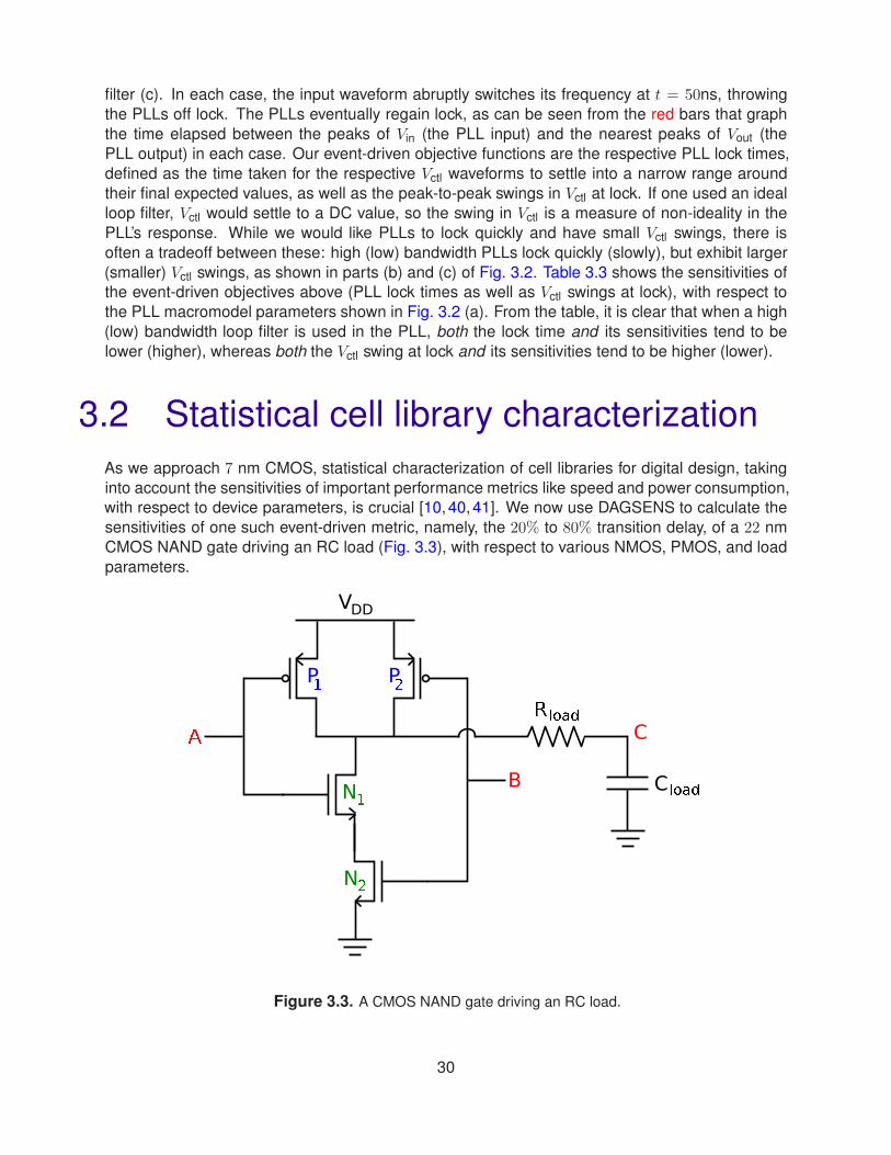
CMOS NAND gate driving an RC load (Fig. 3.3), with respect to various NMOS, PMOS, and load

parameters.

VDD

B

C

P1

P2

N

N!

l"#$

C%&'(

Figure 3.3. A CMOS NAND gate driving an RC load.

30

Figure 3.4. Transient simulation of the CMOS NAND gate of

Fig. 3.3 for two different input transitions, showing the 20% and

80% “transition complete” events, and the corresponding “gate de-lay” objective function in each case.

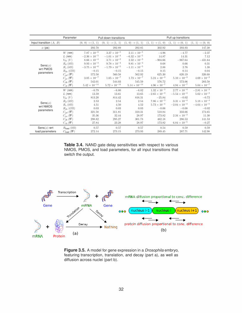
Fig. 3.4 shows 2 transitions of the NAND gate above (while there are 6 possible transitions that

switch the output, we show only 2 to save space, although we analyze the sensitivities of all 6 in

Table 3.4). Fig. 3.4 also shows the “20% complete” and “80% complete” events in each case, as

well as our event-driven gate delay objective function, i.e., the time elapsed between these two

events. Table 3.4 shows the event-driven sensitivities of the NAND gate delay to various NMOS

and PMOS parameters (including widths, lengths, threshold voltages, parasitic resistances and

capacitances, etc.), as well as load parameters. It is interesting to see that, in most (although not

all) cases, the gate delay is more sensitive to PMOS (NMOS) parameters during “pull up” (“pull

down”) transitions, as one would intuitively expect.

3.3 Biological applications

We now apply DAGSENS to a biological example, i.e., gene expression via transcription, trans-

lation, decay, and diffusion in Drosophila embryos (Fig. 3.5) [14, 42]. The system consists of a

Drosophila gene that generates mRNA molecules via transcription, which in turn generate protein

molecules via translation. In parallel, the mRNA and protein molecules also decay. This is all

shown in Fig. 3.5 (a) [14,42]. Also, these reactions take place across multiple sites (called nuclei),

and whenever there is an mRNA/protein concentration difference between two adjacent nuclei,

mRNA/protein molecules flow across nuclei to balance the gap (Fig. 3.5b) [14,42]. In our example,

we have N = 52 nuclei, and each nucleus i (where 1 ≤ i ≤ N ) has an mRNA concentration

[mRNA]i, and a protein concentration [protein]i. The system has a single exponentially decaying

external input u(t) that governs the rate of transcription. The differential-equation model for the

system is:

31

Parameter Pull down transitions Pull up transitions

Input transition (A, B) (0, 0) → (1, 1) (0, 1) → (1, 1) (1, 0) → (1, 1) (1, 1) → (1, 0) (1, 1) → (0, 1) (1, 1) → (0, 0)

φ (ps) 292.70 292.89 292.85 302.92 293.93 147.38

Sens(φ)wrt PMOS

parameters

W (nm) 7.87 × 10−6 3.37 × 10−5 2.11 × 10−5 −4.96 −4.77 −2.37L (nm) −2.36 × 10−5 −1.01× 10−4 −6.32 × 10−5 14.87 14.31 7.12Vth (V ) 8.66 × 10−4 3.71 × 10−3 2.32 × 10−3 −904.66 −867.64 −431.64Rd (kΩ) 9.93 × 10−4 9.78 × 10−4 9.81 × 10−4 0.68 0.66 0.31Rs (kΩ) −3.75 × 10−6 −1.79× 10−5 −1.11 × 10−5 2.88 2.76 1.38Rds (GΩ) −0.15 −0.15 −0.15 0.15 0.14 0.04Cgd (fF) 572.50 560.58 562.92 625.30 620.19 326.68Cgs (fF) 3.05 × 10−7 1.65 × 10−7 1.73 × 10−7 5.24× 10−3 5.10 × 10−3 4.69 × 10−3

Cdb (fF) 542.01 544.03 545.59 576.72 573.06 283.58Csb (fF) 5.42 × 10−14 5.72 × 10−14 5.14 × 10−14 4.96× 10−7 4.94 × 10−7 5.04 × 10−7

Sens(φ)wrt NMOS

parameters

W (nm) −6.79 −6.80 −6.82 1.32× 10−3 2.77 × 10−4 −2.81 × 10−3

L (nm) 13.59 13.61 13.65 −2.65× 10−3 −5.54× 10−4 5.62 × 10−3

Vth (V ) 813.20 814.42 816.31 −25.84 −0.02 −0.72Rd (kΩ) 2.53 2.54 2.54 7.86× 10−3 3.31 × 10−4 5.18 × 10−4

Rs (kΩ) 4.51 4.50 4.52 5.73× 10−4 −2.04× 10−4 −4.64 × 10−5

Rds (GΩ) 0.03 0.03 0.03 −0.06 −0.08 −0.02Cgd (fF) 321.58 311.81 310.31 510.84 333.66 174.65Cgs (fF) 35.36 32.44 28.97 173.82 2.34 × 10−3 11.30Cdb (fF) 298.82 295.27 301.73 462.18 286.53 141.53Csb (fF) 27.84 23.28 28.97 173.82 6.84 × 10−5 −0.27

Sens(φ) wrt

load parameters

Rload (kΩ) 0.57 0.57 0.57 0.54 0.59 0.59Cload (fF) 272.14 273.15 273.93 289.45 287.71 142.98

Table 3.4. NAND gate delay sensitivities with respect to various

NMOS, PMOS, and load parameters, for all input transitions that

switch the output.

Gene m)*+

Protein

Transcription

,r-./034567

Gene

N89:;<=

D>?@B

EFGHI

JKLM(a)

nOPQSUV WXY Z[\]^_` a bcdefgh ijk

opqs tuvusion prwxyz|~ erence

pr usion pr ¡¢£ ¤¥¦erence

(b)

Figure 3.5. A model for gene expression in a Drosophila embryo,

featuring transcription, translation, and decay (part a), as well as

diffusion across nuclei (part b).

32

d

dt[mRNA]i = σmRNA u(t)

︸ ︷︷ ︸

Transcription

+ dmRNA([mRNA]i−1 − [mRNA]i)︸ ︷︷ ︸

Diffusion from previous nucleus

+ dmRNA([mRNA]i+1 − [mRNA]i)︸ ︷︷ ︸

Diffusion from next nucleus

−λmRNA [mRNA]i︸ ︷︷ ︸

Decay

, and (3.1)

d

dt[protein]i = σprotein [mRNA]i

︸ ︷︷ ︸

Translation

+ dprotein([protein]i−1 − [protein]i)︸ ︷︷ ︸

Diffusion from previous nucleus

+ dprotein([protein]i+1 − [protein]i)︸ ︷︷ ︸

Diffusion from next nucleus

−λprotein [protein]i︸ ︷︷ ︸

Decay

, (3.2)

with the understanding that the “diffusion from previous (next) nucleus” term is 0 for the first (last)

(i = 1 (N)) nucleus.

Each nucleus features a maximum [mRNA] event

(a)

Each nucleus features a maximum [protein] event

(b)

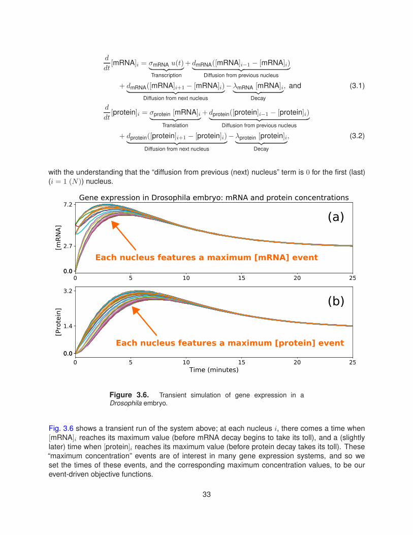
Figure 3.6. Transient simulation of gene expression in aDrosophila embryo.

Fig. 3.6 shows a transient run of the system above; at each nucleus i, there comes a time when

[mRNA]i reaches its maximum value (before mRNA decay begins to take its toll), and a (slightly

later) time when [protein]i reaches its maximum value (before protein decay takes its toll). These

“maximum concentration” events are of interest in many gene expression systems, and so we

set the times of these events, and the corresponding maximum concentration values, to be our

event-driven objective functions.

33

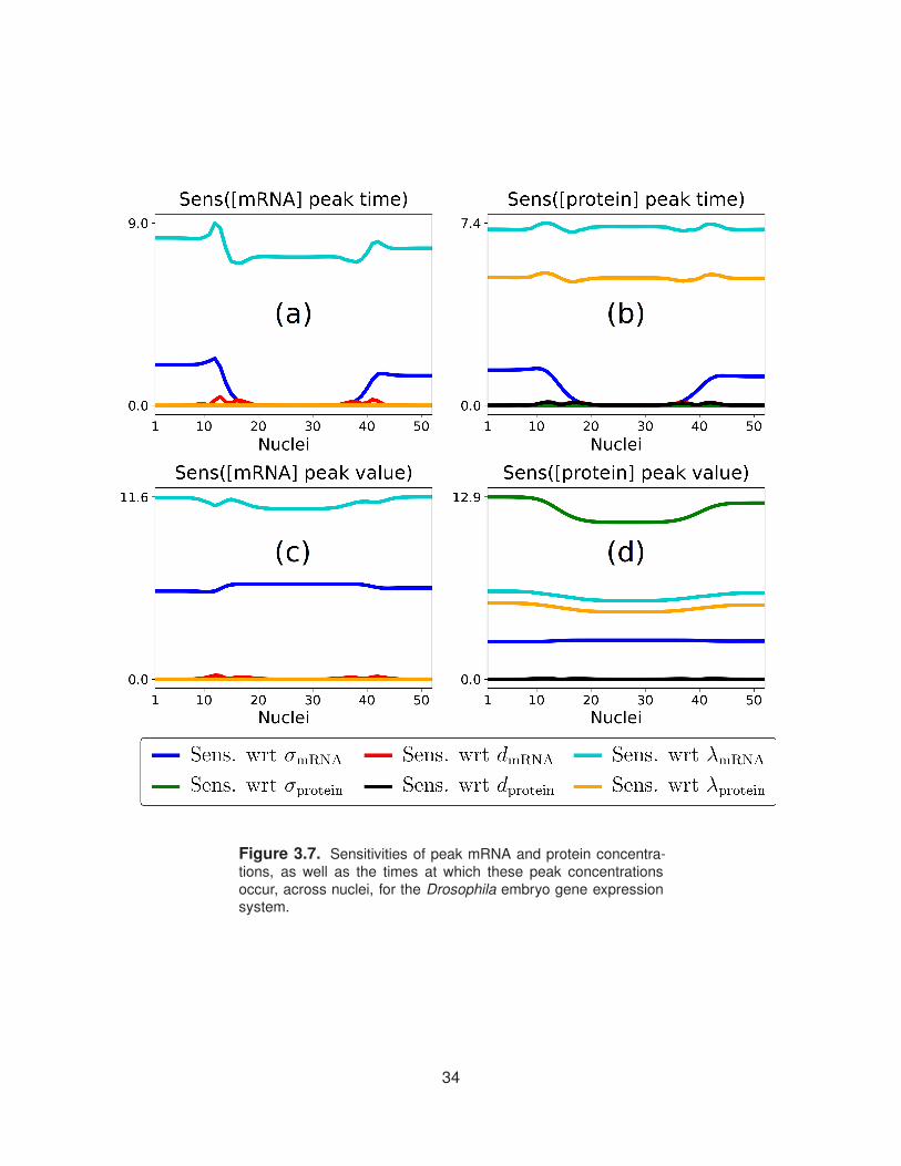
Figure 3.7. Sensitivities of peak mRNA and protein concentra-

tions, as well as the times at which these peak concentrations

occur, across nuclei, for the Drosophila embryo gene expressionsystem.

34

Fig. 3.7 shows a plot of these event-driven sensitivities, across nuclei, with respect to various

system parameters. It is interesting to see that, while the peak mRNA and protein event times, as

well as the peak mRNA concentration value, are all most sensitive to the mRNA decay constant

λmRNA, the peak protein concentration value is most sensitive to the protein translation constant

σprotein, for all the nuclei.

35

4. Summary, Conclusions,

and Future Work

To summarise, we have developed and demonstrated DAGSENS, a simple, elegant, and powerful

theory for transient sensitivity analysis based on directed acyclic graphs. We have also shown

how DAGSENS can be applied to carry out direct and adjoint transient sensitivity analysis of an

entirely new kind of objective function defined based on events that happen during a transient

simulation. We have demonstrated this on several real-world applications including high-speed

communication (with I/O link and PLL examples), statistical cell library characterization, and gene

expression in biological systems.

In future, we would like to significantly improve the DAGSENS code-base, for better CPU and

memory performance; in particular, we would like to migrate DAGSENS from a proof-of-concept

Python implementation to a production-level C++ implementation in the open-source circuit sim-

ulator Xyce R© [22]. We believe that this would also enable us to run DAGSENS on much larger

examples than we can at present.

36

References

[1] J. Nocedal and S. Wright. Numerical optimization. Springer-Verlag, New York, 2006.

[2] A. K. Alekseev, I. M. Navon, and M. E. Zelentsov. The estimation of functional uncertainty

using polynomial chaos and adjoint equations. International Journal for Numerical Methods

in Fluids, 67(3):328–341, 2011.

[3] R. M. Errico. What is an adjoint model? Bulletin of the American Meteorological Society,

78(11):2577–2591, 1997.

[4] Y. Cao and L. Petzold. A posteriori error estimation and global error control for ordinary differ-

ential equations by the adjoint method. SIAM Journal on Scientific Computing, 26(2):359–374,

2004.

[5] S. Director and R. Rohrer. The generalized adjoint network and network sensitivities. IEEE

Transactions on Circuit Theory, 16(3):318–323, 1969.

[6] D. E. Hocevar, P. Yang, T. N. Trick, and B. D. Epler. Transient sensitivity computation for

MOSFET circuits. IEEE Transactions on Electron Devices, 32(10):2165–2176, 1985.

[7] A. R. Conn, P. K. Coulman, R. A. Haring, G. L. Morrill, C. Visweswariah, and C. W. Wu. Jiffy-

Tune: Circuit optimization using time-domain sensitivities. IEEE Transactions on Computer-

Aided Design of Integrated Circuits and Systems, 17(12):1292–1309, 1998.

[8] C. Gu and J. Roychowdhury. An efficient, fully non-linear, variability-aware non-Monte-Carlo

yield estimation procedure with applications to SRAM cells and ring oscillators. In ASPDAC

’08: Proceedings of the 13th Asia and South Pacific Design Automation Conference, pages

754–761, 2008.

[9] I. Stevanovic and . C. C. McAndrew. Quadratic backward propagation of variance for non-

linear statistical circuit modelling. IEEE Transactions on Computer-Aided Design of Integrated

Circuits and Systems, 28(9):1428–1432, 2009.

[10] B. Gu, K. Gullapalli, Y. Zhang, and S. Sundareswaran. Faster statistical cell characteriza-

tion using adjoint sensitivity analysis. In CICC ’08: Proceedings of the 30th Annual Custom

Integrated Circuits Conference, pages 229–232, 2008.

[11] T. Turanyi. Sensitivity analysis in chemical kinetics. International Journal of Chemical Kinetics,

40(11):685–686, 2008.

[12] T. Ziehn and A. S. Tomlin. GUI–HDMR: A software tool for global sensitivity analysis of

complex models. Environmental Modelling & Software, 24(7):775–785, 2009.

37

[13] J. M. Dresch, X. Liu, D. N. Arnosti, and A. Ay. Thermodynamic modelling of transcription: Sen-

sitivity analysis differentiates biological mechanism from mathematical model-induced effects.

BMC Systems Biology, 4(1):142, 2010.

[14] G. D. McCarthy, R. A. Drewell, and J. M. Dresch. Global sensitivity analysis of a dynamic

model for gene expression in Drosophila embryos. PeerJ, 3:e1022, 2015.

[15] M. Morohashi, A. E. Winn, M. T. Borisuk, H. Bolouri, J. Doyle, and H. Kitano. Robustness as

a measure of plausibility in models of biochemical networks. Journal of Theoretical Biology,

216(1):19–30, 2002.

[16] T. Eissing, F. Allgower, and E. Bullinger. Robustness properties of apoptosis models with

respect to parameter variations and intrinsic noise. Systems Biology, 152(4):221–228, 2005.

[17] A. Meir and J. Roychowdhury. BLAST: Efficient computation of non-linear delay sensitivities

in electronic and biological networks using barycentric Lagrange enabled transient adjoint

analysis. In DAC ’12: Proceedings of the 49th Annual Design Automation Conference, pages

301–310, 2012.

[18] Y. Cao, S. Li, L. Petzold, and R. Serban. Adjoint sensitivity analysis for differential-algebraic

equations: The adjoint DAE system and its numerical solution. SIAM Journal on Scientific

Computing, 24(3):1076–1089, 2003.

[19] F. Y. Liu and P. Feldmann. A time-unrolling method to compute sensitivity of dynamic systems.

In DAC ’14: Proceedings of the 51st Annual Design Automation Conference, 2014.

[20] R. Bartlett. A derivation of forward and adjoint sensitivities for ODEs and DAEs. Technical

Report SAND2007-6699, Sandia National Laboratories, Albuquerque, NM, USA, 2008.

[21] Synopsys. HSPICE R© user guide: Simulation and analysis, 2010.

[22] E. R. Keiter, K. V. Aadithya, T. Mei, T. V. Russo, R. L. Schiek, P. E. Sholander, H. K. Thornquist,

and J. C. Verley. Xyce R© parallel electronic simulator (v6.6): User’s guide. Technical Report

SAND2016-11716, Sandia National Laboratories, Albuquerque, NM, USA, 2016.

[23] J. Kleinberg and E. Tardos. Algorithm design. Pearson Education, 2006.

[24] C. E. Leiserson, R. L. Rivest, C. Stein, and T. H. Cormen. Introduction to algorithms. The

MIT Press, 2001.

[25] A. Griewank and A. Walther. Evaluating derivatives: Principles and techniques of algorithmic

differentiation. SIAM, 2008.

[26] C. H. Bischof, P. D. Hovland, and B. Norris. On the implementation of automatic differentiation

tools. Higher-Order and Symbolic Computation, 21(3):311–331, 2008.

[27] J. Roychowdhury. Numerical simulation and modelling of electronic and biochemical systems.

Foundations and Trends in Electronic Design Automation, 3(2–3):97–303, 2009.

[28] L. W. Nagel. SPICE2: A computer program to simulate semiconductor circuits. PhD thesis,

UC Berkeley, 1975.

[29] L. Edelstein-Keshet. Mathematical models in biology. SIAM, 2005.

38

[30] A. L. Sangiovanni-Vincentelli. Computer Design Aids for VLSI Circuits, chapter Circuit Simu-

lation, pages 19–112. Springer, Netherlands, 1984.

[31] L. O. Chua and P. M. Lin. Computer-aided analysis of electronic circuits: Algorithms and

computational techniques. 1975.

[32] H. Shichman. Integration system of a non-linear transient network analysis program. IEEE

Transactions on Circuit Theory, 17(3):378–386, 1970.

[33] C. W. Gear. The numerical integration of ordinary differential equations. Mathematics of

Computation, 21(98):146–156, 1967.

[34] R. E. Bryant. Symbolic Boolean manipulation with ordered binary-decision diagrams. ACM

Computing Surveys, 24(3):293–318, 1992.

[35] G. Balamurugan, B. Casper, J. E. Jaussi, M. Mansuri, F. O’Mahony, and J. Kennedy. Modelling

and analysis of high-speed I/O links. IEEE Transactions on Advanced Packaging, 32(2):237–

247, 2009.

[36] P. K. Hanumolu, G. Y. Wei, and U. K. Moon. Equalizers for high-speed serial links. Interna-

tional Journal of High Speed Electronics and Systems, 15(2):429–458, 2005.

[37] J. A. Davis and J. D. Meindl. Interconnect technology and design for gigascale integration.

Springer, Netherlands, 2003.

[38] B. Razavi. Design of analog CMOS integrated circuits. Tata McGraw-Hill Publishing Company

Ltd., New Delhi, India, 2001.

[39] J. L. Stensby. Phase-locked loops: Theory and applications. CRC Press, 1997.

[40] A. Goel and S. Vrudhula. Statistical waveform and current source based standard cell models

for accurate timing analysis. In DAC ’08: Proceedings of the 45th Annual Design Automation

Conference, pages 227–230, 2008.

[41] L. Yu, S. Saxena, C. Hess, I. M. Elfadel, D. Antoniadis, and D. Boning. Statistical library

characterization using belief propagation across multiple technology nodes. In DATE ’15:

Proceedings of the 18th Design, Automation & Test Conference in Europe, pages 1383–1388,

2015.

[42] J. M. Dresch, M. A. Thompson, D. N. Arnosti, and C. Chiu. Two-layer mathematical modelling

of gene expression: Incorporating DNA-level information and system dynamics. SIAM Journal

on Applied Mathematics, 73(2):804–826, 2013.

39

DISTRIBUTION:

1 MS 0899 Technical Library, 9536 (electronic copy)

40

v1.40

41

42