sensitivity analysis: the direct and adjoint method - jku · sensitivity analysis: the direct and...
TRANSCRIPT
J OH AN N E S K EP LE RU N I VE R S I T AT L I N Z
N e t zw e r k f u r F o r s c h u n g , L e h r e u n d P r a x i s
Sensitivity Analysis: The Direct and AdjointMethod
Masterarbeit
zur Erlangung des akademischen Grades
Diplomingenieur
in der Studienrichtung
Industriemathematik
Angefertigt am Institut fur Numerische Mathematik
Betreuung:
A. Univ.-Prof. Dipl.-Ing. Dr. Walter Zulehner
Eingereicht von:
Markus Kollmann
Linz, Februar 2010
Johannes Kepler UniversitatA-4040 Linz · Altenbergerstraße 69 · Internet: http://www.uni-linz.ac.at · DVR 0093696

Abstract
Shape optimization is widely used in practice. The typical problem is tofind the optimal shape which minimizes/maximizes a certain cost functionaland satisfies some given constraints. Usually shape optimization problemsare solved numerically, by some iterative method which also requires somegradient information.There are two approaches to provide such information: the direct approachand the adjoint approach.In this thesis the different approaches, for getting gradient information of thefunctional, will be presented and then the focus is to compare them. It willbe shown that the adjoint approach has a great advantage, but that therealso exist examples, where the adjoint technique does not work in the sensewe will introduce it.
Starting with the explanation of shape optimization, the direct and adjointapproach will be introduced. Then an introduction in shape derivatives isgiven and some necessary examples for them are shown.On the basis of a two-dimensional magnetostatic field problem, where themathematical model is derived using Maxwell’s equations, and is the varia-tional formulation of a boundary value problem, the process of getting gra-dient information will be shown.Finally, numerical results illustrate the two approaches.
i

Zusammenfassung
Formoptimierung ist ein weit verbreitetes Gebiet der Optimierung. Das Pro-blem besteht darin, eine optimale Form (Geometrie) zu finden, die ein gegebe-nes Zielfunktional minimiert/maximiert und vorgegebene Nebenbedingungenerfullt. Solche Probleme werden meistens mit iterativen Verfahren numerischgelost und diese Verfahren benotigen Gradienteninformation.Um diese zu bewerkstelligen gibt es zwei Methoden: die direkte Methode unddie adjungierte Methode.In dieser Arbeit werden die beiden Zugange, um Information uber den Gra-dienten des Funktionals zu bekommen, aufgezeigt und dann liegt der Fokusdarin, die Methoden zu vergleichen. Es wird sich herausstellen, dass der ad-jungierte Zugang einen großen Vorteil besitzt, es aber auch Beispiele existie-ren, wo er nicht anwendbar ist.
Zuerst folgt eine Erklarung der Idee der Formoptimierung und die direkteund adjungierte Methode werden erlautert. Dann wird eine Einfuhrung indie Theorie der shape derivatives gegeben und einige wichtige Beispiele wer-den prasentiert.Auf Basis eines zweidimensionalen magnetostatischen Feldproblems, bei demdas mathematische Modell mithilfe der Maxwell Gleichungen hergeleitet wird(Variationsformulierung eines Randwertproblems), werden die Methoden ge-zeigt.Zum Schluss werden numerische Resultate die beiden Methoden veranschau-lichen.
ii

Acknowledgement
First of all, I would like to express my thanks to my supervisor Prof. W.Zulehner, for giving me the chance to write this thesis, for his guidance andsuggestions on this work; especially, thanks for the providing me with theknowledge on shape derivatives.
I also want to thank my colleagues, especially Stefan Muhlbock and LisaFrank for the valuable contributions.
Last but not least I want to thank my father for giving me the possibil-ity to study and my girlfriend Sylvia for the mental assistance.
This work has been carried out at the Institute of Computational Mathe-matics, JKU Linz.
iii
Contents
1 Introduction 1
2 The Idea of Shape Optimization 32.1 Motivation . . . . . . . . . . . . . . . . . . . . . . . . . . . . . 32.2 An Optimal Shape Design Problem . . . . . . . . . . . . . . . 32.3 The Direct and Adjoint Method in the Discrete Setting . . . . 4
2.3.1 The Direct Method . . . . . . . . . . . . . . . . . . . . 52.3.2 The Adjoint Method . . . . . . . . . . . . . . . . . . . 5
2.4 The Direct and Adjoint Method in the Continuous Setting . . 62.4.1 The Direct Method . . . . . . . . . . . . . . . . . . . . 72.4.2 The Adjoint Method . . . . . . . . . . . . . . . . . . . 7
3 Introduction to Shape Derivatives 93.1 The Geometry . . . . . . . . . . . . . . . . . . . . . . . . . . . 93.2 Shape Functionals . . . . . . . . . . . . . . . . . . . . . . . . . 10
3.2.1 Domain Integrals . . . . . . . . . . . . . . . . . . . . . 113.2.2 Boundary Integrals . . . . . . . . . . . . . . . . . . . . 14
4 Derivation of the Physical Problem 184.1 Physical Model . . . . . . . . . . . . . . . . . . . . . . . . . . 18
4.1.1 Maxwell’s Equations . . . . . . . . . . . . . . . . . . . 184.2 Mathematical Model . . . . . . . . . . . . . . . . . . . . . . . 20
4.2.1 Reduction to 2D . . . . . . . . . . . . . . . . . . . . . 204.2.2 Variational Formulation . . . . . . . . . . . . . . . . . 234.2.3 Existence and Uniqueness . . . . . . . . . . . . . . . . 25
4.3 The Cost Functional . . . . . . . . . . . . . . . . . . . . . . . 27
5 Shape Derivative Analysis for the Physical Problem 295.1 The Eulerian Derivative of the Cost Functional . . . . . . . . 295.2 The Boundary Value Problem for the Shape Derivative . . . . 31
5.2.1 The Direct Approach . . . . . . . . . . . . . . . . . . . 385.2.2 The Adjoint Approach . . . . . . . . . . . . . . . . . . 38
5.3 The Test Problem . . . . . . . . . . . . . . . . . . . . . . . . . 40
iv
6 Discretization 456.1 Introduction to the Finite Element Method . . . . . . . . . . . 456.2 The Finite Element Method applied to the Test Problem . . . 486.3 The CG - Method . . . . . . . . . . . . . . . . . . . . . . . . . 50
7 Numerical Results 527.1 The Analytical Solutions . . . . . . . . . . . . . . . . . . . . . 527.2 Comparison of the Direct and Adjoint Method . . . . . . . . . 53
8 Conclusions and Outlook 648.1 Conclusion . . . . . . . . . . . . . . . . . . . . . . . . . . . . . 648.2 Outlook . . . . . . . . . . . . . . . . . . . . . . . . . . . . . . 64
Bibliography 66
Eidesstattliche Erklarung 68
Curriculum Vitae 69
v
Chapter 1
Introduction
The thesis deals with the usage of the so-called shape derivatives in shapeoptimization. The whole thesis is mainly based on the books from Haslingerand Makinen [1], Sokolowski and Zolesio [2] and Delfour and Zolesio [3] (someparts can also be found in the book from Le Tallec and Laporte [4]).In this books one can find the mathematical approach for introducing shapederivatives and working with it. In this thesis the concentration is abouton how to calculate and work with shape derivatives and not about all theassumptions which have to be satisfied. It is assumed that everything issmooth enough, well defined and exists. So in this thesis it is shown howsomeone can work with shape derivatives.
The tasks of this thesis:
In this thesis we want to get an idea of the behaviour of two different ap-proaches (direct and adjoint method) for shape optimization by analysing atwo-dimensional problem. This happens in the following way:
• Use the direct method for getting gradient information of some costfunctional.
• Introduce the adjoint technique and use it for the task of providinggradients.
• Compare the results of these two methods and draw conclusions.
The organization of this thesis:
• Chapter 1 is the introduction.
• In chapter 2 the idea of shape optimization is introduced and the termshape optimization problem is defined. It will turn out that gradients
1
have to be calculated. For this, two possible approaches are presented:the direct approach and the adjoint approach. The details of thesemethods will be worked out for the discrete and the continuous case.
• In chapter 3 some basic knowledge about shape derivatives is intro-duced, especially the definition of the change of the geometry of somebounded Lipschitz domain Ω ⊆ RN . Then the term Eulerian derivative(directional derivative of a functional) is defined and some examples forthis follow. So with this it will be shown how to compute the derivativewith respect to the change of the geometry of domain- and boundary-integrals.
• In chapter 4 from the physical model for magnetostatics, i.e. Maxwell’sequations, the mathematical model is derived, which is then the varia-tional formulation of a boundary value problem for a partial differentialequation. Then the cost functional, which describes the torque, is de-rived and will depend on the solution of the boundary value problem.
• In chapter 5 a variational formulation for the shape derivative is derivedout of the given variational formulation of the boundary value problemfrom chapter 4 using the techniques introduced in chapter 3. Thenthe direct and adjoint approach are figured out for the (in chapter 4)derived problem.
• In chapter 6 we give a short introduction to the finite element method(FEM). After applying it to the test problem, we shortly introducethe conjugate gradient method (CG method), with which we solve theresulting linear systems.
• In chapter 7 the numerical results for the direct and adjoint methodare presented and compared.
• In chapter 8 the results are summarized and conclusions about possiblecontinuations are drawn.
2

Chapter 2
The Idea of Shape Optimization
In this chapter the whole idea and principle of shape optimization is in-troduced (as one can find it in [1] and [5]). This will lead us then to twoapproaches which are presented: the direct method and the adjoint method(see also [6]). There the so-called shape derivatives appear, which are thenformally introduced in chapter 3.
2.1 Motivation
The typical aim of a shape optimization problem is to modify the shape ofan object in such a way that the resulting object is optimal with respectto a certain criterion. This criterion is usually some sort of cost functionalwhich then has to be minimized or maximized. Since any minimizationproblem can be easily written as a maximization problem and vice versa,only maximization problems are considered.In most of the cases the functional itself is depending on a variable which isthe solution of a state problem and given through equations.
2.2 An Optimal Shape Design Problem
Definition 2.1 Let O be a family of admissible domains Ω ⊆ RN , Ω thedomain for the state problem and u(Ω) the solution of the state problem.Then the graph of the optimal shape design problem is defined as the set:
G := (Ω, u(Ω))|Ω ∈ O.
Now let I(Ω, u(Ω)) with I : G→ R be the cost functional and setJ(Ω) = I(Ω, u(Ω)). Then the optimal shape design problem can be writtenas:
Find Ω∗ ∈ O : J(Ω∗) ≥ J(Ω) for all Ω ∈ O. (2.1)
3

If the shape is given through a parametrization we have the following defini-tion:
Definition 2.2 Let P be a family of admissible parameters, P ⊆ Rk,Ω = Ω(p) the domain for the state problem with p ∈ P and u(p) = u(Ω(p))the solution of the state problem. Then the graph of the optimal shape designproblem for parameterized shapes is defined as the set:
G := (p, u(p))|p ∈ P.
Now let again I(p, u(p)) with I : G → R be the cost functional and setJ(p) = I(p, u(p)). Then the optimal shape design problem for parameterizedshapes can be written as:
Find p∗ ∈ P : J(p∗) ≥ J(p) for all p ∈ P . (2.2)
The kind and number of design parameters is depending on the problem.
In the next sections the direct and adjoint methods will be introduced inthe discrete and continuous setting but the finite element method for dis-cretization will be discussed in detail in chapter 6. So for now only someresults from the finite element method are used which will be discussed in alater chapter.
2.3 The Direct and Adjoint Method in the
Discrete Setting
Assume that the state problem is already discretized and reads as follows:
Find u ∈ RNp : K(p)u(p) = f(p), (2.3)
where K is a sparse matrix.Additionally, consider the shape design problem (2.2) with constraintscl(p, u(p)) ≤ 0, where l = 1, ...,M and M is the number of constraints.
So in short the following problem has to be solved (with the settingcl(p) = cl(p, u(p))):
J(p)→ maxp∈Rk
(2.4)
cl(p) ≤ 0.
4

In optimization routines the gradients of J and c are needed and they lookas follows:
dJ
dpi
=∂I
∂pi
+∂I
∂u· ∂u
∂pi
, (2.5)
dcl
dpi
=∂cl
∂pi
+∂cl
∂u· ∂u
∂pi
,
where i = 1, ..., k and l = 1, ...,M .
The quantities ∂u/∂pi are called sensitivities.
For calculating these gradients the special structure of the state equation(Ku = f) is exploited and leads to two approaches: the direct method andthe adjoint method.
2.3.1 The Direct Method
Differentiation of the state equation with respect to pi gives:
∂(Ku)
∂pi
=∂f
∂pi
which is equivalent to
∂K
∂pi
u + K∂u
∂pi
=∂f
∂pi
or, equivalently
K∂u
∂pi
=∂f
∂pi
− ∂K
∂pi
u. (2.6)
The idea is now to solve (2.6) with respect to ∂u/∂pi and use this solutionfor the calculation of the gradients of J and cl in (2.5).
Therefore, for each design parameter pi one solution of problem (2.6) isneeded.
2.3.2 The Adjoint Method
We have
∂u
∂pi
= K−1( ∂f
∂pi
− ∂K
∂pi
u)
(2.7)
5
Then for the calculation of the gradients of J and cl we obtain:
dJ
dpi
=∂I
∂pi
+∂I
∂u·K−1
( ∂f
∂pi
− ∂K
∂pi
u)
=∂I
∂pi
+ K−T ∂I
∂u·( ∂f
∂pi
− ∂K
∂pi
u),
dcl
dpi
=∂cl
∂pi
+∂cl
∂u·K−1
( ∂f
∂pi
− ∂K
∂pi
u)
=∂cl
∂pi
+ K−T ∂cl
∂u·( ∂f
∂pi
− ∂K
∂pi
u),
where i = 1, ..., k and l = 1, ...,M .
Now adjoint variables λ = (λ1, ..., λM+1)T are defined by
KT λ1 =∂I
∂u, (2.8)
KT λl+1 =∂cl
∂u.
The problem (2.8) is called the adjoint state problem.Plugging this into the formulas for calculating the gradients of J and cl leadsto
dJ
dpi
=∂I
∂pi
+ λ1 ·( ∂f
∂pi
− ∂K
∂pi
u), (2.9)
dcl
dpi
=∂cl
∂pi
+ λl+1 ·( ∂f
∂pi
− ∂K
∂pi
u).
Compared to the direct approach, where we need one solution of the dif-ferentiated state problem (2.6) for each design parameter pi, here only onesolution of the adjoint state problem (2.8) is needed for the objective andeach restriction.
In the next section it is shown how to set up the approaches in the con-tinuous setting.
2.4 The Direct and Adjoint Method in the
Continuous Setting
Assume that the state problem is of the following form:
Find u ∈ V : a(u, v) = 〈F, v〉 , ∀v ∈ V, (2.10)
6

with an appropriate Hilbert space V , a bilinear form a(., .) and a linear form〈F, .〉 = F (.). Or, in operator notation
Find u ∈ V : Au = F. (2.11)
Additionally, consider again problem (2.4) but for simplicity we assume thatthe functional and the constraints are not explicitly depending on the pa-rameter p, i.e. J(p) = I(u(p)) and cl(p) = cl(u(p)), and that there is onlyone design parameter:
J(p)→ maxp∈R
cl(p) ≤ 0.
Again the calculation of the gradients of the objective functional and theconstraints is needed. In chapter 3 we will see that these gradients are linearfunctionals of the following form:
dJ = 〈f1, u′〉 , (2.12)
dcl = 〈fl+1, u′〉 ,
where l = 1, ...,M and u′ denotes the so-called shape derivative.
2.4.1 The Direct Method
By important techniques involving shape derivatives (see chapter 3) it ispossible to derive an equation for the unknown shape derivative u′ out of theequation for the state problem (2.10):
Find u′ ∈ V : a′(u′, v) = 〈F ′, v〉 , ∀v ∈ V, (2.13)
where the bilinear form a′(., .) is derived by differentiating the bilinear formin (2.10) and the linear form 〈F ′, .〉 is derived by differentiating the linearform in (2.10) (see chapter 3) . Again in operator notation
Find u′ ∈ V : A′u′ = F ′. (2.14)
The idea is now to solve (2.13) and use this solution for the calculation ofthe gradients of J and cl in (2.12).
2.4.2 The Adjoint Method
The shape derivative u′ is determined as the solution of the following problem:
Find u′ ∈ V : 〈A′u′, v〉 = 〈F ′, v〉 , ∀v ∈ V.
7

Now the adjoint variables λ = (λ1, ..., λM+1)T are defined straight forward
by the following adjoint problem
Find λ ∈ (V )M+1 : 〈(A′)∗λ1, w〉 = 〈f1, w〉 , ∀w ∈ V, (2.15)
〈(A′)∗λl+1, w〉 = 〈fl+1, w〉 , ∀w ∈ V.
where (A′)∗ denotes the adjoint of A′.
As u′ is an element in V we have
〈(A′)∗λ1, u′〉 = 〈λ1, A
′u′〉 = 〈F ′, λ1〉 ,〈(A′)∗λl+1, u
′〉 = 〈λl+1, A′u′〉 = 〈F ′, λl+1〉
and therefore
dJ = 〈F ′, λ1〉 , (2.16)
dcl = 〈F ′, λl+1〉 .
where l = 1, ...,M .
Both approaches can be extended to problems with more than one designparameter. Then, in the direct approach, for each parameter we have tosolve one differentiated state problem for the shape derivative. In the ad-joint approach only one solution of the adjoint state problem is needed forthe objective and each restriction.
8

Chapter 3
Introduction to ShapeDerivatives
In this chapter the basic knowledge in shape derivatives is presented basedon the material derivative idea of continuum mechanics (see also [7] and [8]).This presentation will be formal, meaning that it is correct provided that alldata we need are sufficiently smooth.As seen in chapter 2, shape optimization deals with computations of deriva-tives of solutions to state problems as well as cost functionals with respectto shape variations. Here it will be shown, how to compute the derivative ofa functional (Eulerian derivative) using shape derivatives.
3.1 The Geometry
We want to study the geometric change of a bounded domain Ω ⊆ RN ,N ∈ N, with Lipschitz boundary ∂Ω. Ω is thought to be a collection of ma-terial particles changing their position in time. The space occupied by themat time t will determine a new configuration Ωt. The change in the geom-etry of Ω will be given by a process which deforms the initial configuration Ω.
To formalize this mathematically, let
Tt : Ω→ RN , t ∈ [0, ε)
be a family of transformations, which describes the motion of each materialparticle in the domain Ω:
X ∈ Ω 7→ x = Tt(X) ≡ x(t,X)
such that
T0(Ω) = Ω
9
i.e., T0 = identity.
The transformed geometry is given by:
Ωt = Tt(Ω)
i.e., Ωt is the image of Ω with respect to Tt.
Like in continuum mechanics we assume Tt to be a one-to-one transformationof Ω onto Ωt, such that
Tt (intΩ) = intΩt, Tt(∂Ω) = ∂Ωt.
The point X may be thought of as the Lagrangian coordinates while x arethe Eulerian coordinates of a particle.
Remark 3.1 In our purposes the parameter t will not be time but describesthe amount of change of the geometry.
Definition 3.2 The Eulerian velocity field V (t, x) at the point x(t) is givenby:
V (t, x) =∂x
∂t(t, T−1
t (x)).
By this definition one can see, that x(t,X) satisfies the following initial valueproblem
d
dtx(t,X) = V (t, x(t,X)) (3.1)
x(0, X) = X
and, vice versa, for each V (t, x) the family of transformations Tt(V )(X) canbe determined as solution of the problem (3.1).
3.2 Shape Functionals
In this section the so-called Eulerian derivative is introduced, calculated fordomain and boundary integrals and the term shape derivative is defined.
Definition 3.3 Let Ω ⊆ RN be a bounded Lipschitz domain and let J be afunctional with Ω 7→ J(Ω). Then the Eulerian derivative of the functional Jat Ω in the direction of a vector field V is given by:
dJ(Ω; V ) =d
dtJ(Ωt)
∣∣∣∣t=0
= limt↓0
1
t(J(Ωt)− J(Ω)) (3.2)
with Ωt = Tt(V )(Ω).
10
The Eulerian derivative is a directional derivative for the, in this sense oftencalled, shape functional J .
In the next subsections the Eulerian derivative of some important examplesof functionals is calculated. Let Γ = ∂Ω.
3.2.1 Domain Integrals
Consider
J(Ω) =
∫Ω
F (x, y(Ω)(x),∇y(Ω)(x)) dx,
where F : Ω× R× RN → R, (x, y, p) 7→ F (x, y, p).
Then
J(Ωt) =
∫Ωt
F (x, y(Ωt)(x),∇y(Ωt)(x)) dx.
Transforming the integral to an integral over Ω (substitution rule) leads to
J(Ωt) =
∫Ω
F (Tt(x), (y(Ωt) Tt)(x), (DT−Tt (x)∇(y(Ωt) Tt)(x)))det(DTt(x)) dx
with DTt = (∂Tt,i(V )
∂Xj(X))i,j=1,...,N .
With (3.2) we have
dJ(Ω; V ) =d
dtJ(Ωt)
∣∣∣∣t=0
=d
dt
∫Ω
F (Tt(x), (y(Ωt) Tt)(x), (DT−Tt (x)∇(y(Ωt) Tt)(x)))γ(t)(x) dx
∣∣∣∣t=0
with γ(t)(x) := det(DTt(x)).It can be easily shown that γ(0)(x) = 1.
Since the domain of integration does not depend on t anymore we can inter-change the order of differentiation and integration and get
dJ(Ω; V )
=
∫Ω
d
dt
[F (Tt(x), (y(Ωt) Tt)(x), (DT−T
t (x)∇(y(Ωt) Tt)(x)))γ(t)(x)]∣∣∣∣
t=0
dx.
11
Product rule and chain rule for differentiation leads to
dJ(Ω; V ) =
∫Ω
F (x, y(Ω)(x),∇y(Ω)(x))γ′(0)(x) dx
+
∫Ω
∇xF (x, y(Ω)(x),∇y(Ω)(x)) · V (0, x) dx
+
∫Ω
DyF (x, y(Ω)(x),∇y(Ω)(x))y(Ω; V )(x) dx
+
∫Ω
DpF (x, y(Ω)(x),∇y(Ω)(x)) · ˙(∇y)(Ω; V )(x) dx
+
∫Ω
DpF (x, y(Ω)(x),∇y(Ω)(x))d
dt
[DT−T
t (x)]∣∣∣∣
t=0
∇y(Ω)(x) dx
with
V (0, x) :=dTt(x)
dt
∣∣∣∣t=0
, (3.3)
the material derivative
y(Ω; V )(x) :=d
dt
[(y(Ωt) Tt)(x)
]∣∣∣∣t=0
(3.4)
and where v · w denotes the Euclidean inner product in RN . Dy (resp. Dp)denotes the derivative with respect to y (resp. p).
It can be shown that (proof: see [2, page 76])
γ′(0)(x) = divV (0, x) (3.5)
and
d
dt
[DT−T
t (x)]∣∣∣∣
t=0
= −DV T (0, x). (3.6)
Under certain smoothness assumptions the material and spatial derivativescommute:
˙(∇y)(Ω; V ) = ∇y(Ω; V ).
12

With this we have
dJ(Ω; V ) =
∫Ω
F (x, y(Ω)(x),∇y(Ω)(x))divV (0, x) dx
+
∫Ω
∇xF (x, y(Ω)(x),∇y(Ω)(x)) · V (0, x) dx
+
∫Ω
DyF (x, y(Ω)(x),∇y(Ω)(x))y(Ω; V )(x) dx
+
∫Ω
DpF (x, y(Ω)(x),∇y(Ω)(x)) · ∇y(Ω; V )(x) dx
−∫
Ω
DpF (x, y(Ω)(x),∇y(Ω)(x))DV T (0, x)∇y(Ω)(x) dx.
Now we introduce the so called shape derivative y′(Ω; V ):
Definition 3.4 The shape derivative of y(Ω) in the direction V is given by:
y′(Ω; V )(x) := y(Ω; V )(x)−∇y(Ω)(x) · V (0, x). (3.7)
Using this definition we have
∇y(Ω; V )(x) = ∇y′(Ω; V )(x) +∇[∇y(Ω)(x) · V (0, x)
]= ∇y′(Ω; V )(x) + DV T (0, x)∇y(Ω)(x) + (V (0, x) · ∇)∇y(Ω)(x).
Therefore,
∇y(Ω; V )(x)−DV T (0, x)∇y(Ω)(x) = ∇y′(Ω; V )(x) + (V (0, x) · ∇)∇y(Ω)(x)
and
dJ(Ω; V ) =
∫Ω
F (x, y(Ω)(x),∇y(Ω)(x))divV (0, x) dx
+
∫Ω
∇xF (x, y(Ω)(x),∇y(Ω)(x)) · V (0, x) dx
+
∫Ω
DyF (x, y(Ω)(x),∇y(Ω)(x))y′(Ω; V )(x) dx
+
∫Ω
DyF (x, y(Ω)(x),∇y(Ω)(x))(V (0, x) · ∇)y(Ω)(x) dx
+
∫Ω
DpF (x, y(Ω)(x),∇y(Ω)(x)) · ∇y′(Ω; V )(x) dx
+
∫Ω
DpF (x, y(Ω)(x),∇y(Ω)(x)) · (V (0, x) · ∇)∇y(Ω)(x) dx.
13

Since
div[F (x, y(x), p(x))V (x)
]= F (x, y(x), p(x))divV (x) + Dx
[F (x, y(x), p(x))
]· V (x)
= F (x, y(x), p(x))divV (x) +∇xF (x, y(x), p(x)) · V (x)
+ DyF (x, y(x), p(x))∇xy(x) · V (x) + DpF (x, y(x), p(x))Dxp(x)V (x)
= F (x, y(x), p(x))divV (x) +∇xF (x, y(x), p(x)) · V (x)
+ DyF (x, y(x), p(x))(V (x) · ∇)y(x) + DpF (x, y(x), p(x)) · (V (x) · ∇)p(x),
we finally obtain
dJ(Ω; V ) =
∫Ω
DyF (x, y(Ω)(x),∇y(Ω)(x))y′(Ω; V )(x) dx
+
∫Ω
DpF (x, y(Ω)(x),∇y(Ω)(x)) · ∇y′(Ω; V )(x) dx
+
∫Ω
div[F (x, y(Ω)(x),∇y(Ω)(x))V (0, x)
]dx,
or, by using Gauss’ theorem
dJ(Ω; V ) =
∫Ω
DyF (x, y(Ω)(x),∇y(Ω)(x))y′(Ω; V )(x) dx (3.8)
+
∫Ω
DpF (x, y(Ω)(x),∇y(Ω)(x)) · ∇y′(Ω; V )(x) dx
+
∫Γ
F (x, y(Ω)(x),∇y(Ω)(x))V (0, x) · n(x) ds.
3.2.2 Boundary Integrals
Consider
J(Γ) =
∫Γ
F (x, y(Ω)(x),∇y(Ω)(x)) ds,
where F : Ω× R× RN → R, (x, y, p) 7→ F (x, y, p).
Then
J(Γt) =
∫Γt
F (x, y(Ωt)(x),∇y(Ωt)(x)) ds.
Transforming the boundary integral to an integral over Γ (substitution rule)leads to
J(Γt) =
∫Γ
F (Tt(x), (y(Ωt) Tt)(x), (DT−Tt (x)∇(y(Ωt) Tt)(x)))ω(t)(x) ds
14
with
ω(t)(x) = γ(t)(x)‖DT−Tt (x)n(x)‖l2 .
We have (interchanging differentiation and integration)
d
dtJ(Γt)
∣∣∣∣t=0
=
∫Γ
d
dt
[F (Tt(x), (y(Ωt) Tt)(x), (DT−T
t (x)∇(y(Ωt) Tt)(x)))ω(t)(x)]∣∣∣∣
t=0
ds.
It can be shown that (proof: see [2, page 80])
ω′(0)(x) = divV (0, x)−DV (0, x)n(x) · n(x). (3.9)
Definition 3.5 Let Ω be a bounded Lipschitz domain with the boundary Γand V a vector field. Then the tangential divergence is defined as
divΓV := divV −DV n · n.
With this we have
d
dtJ(Γt)
∣∣∣∣t=0
=
∫Γ
F (x, y(Ω)(x),∇y(Ω)(x))divΓV (0, x) ds
+
∫Γ
∇xF (x, y(Ω)(x),∇y(Ω)(x)) · V (0, x) ds
+
∫Γ
DyF (x, y(Ω)(x),∇y(Ω)(x))y′(Ω; V )(x) ds
+
∫Γ
DyF (x, y(Ω)(x),∇y(Ω)(x))V (0, x) · ∇y(Ω)(x) ds
+
∫Γ
DpF (x, y(Ω)(x),∇y(Ω)(x)) · ∇y′(Ω; V )(x) ds
+
∫Γ
DpF (x, y(Ω)(x),∇y(Ω)(x)) · (V (0, x) · ∇)∇y(Ω)(x) ds.
Definition 3.6 The tangential gradient of y in a point of Γ is defined as:
∇Γy = ∇y − ∂y
∂nn. (3.10)
Remark 3.7 For the tangential gradient of y the following holds:∫Γ
∇Γy ·W dΓ = −∫
Γ
ydivΓW dΓ (3.11)
∀W with W · n = 0 on Γ.
15

Using (3.10) we get
d
dtJ(Γt)
∣∣∣∣t=0
=
∫Γ
F (x, y(Ω)(x),∇y(Ω)(x))divΓV (0, x) ds
+
∫Γ
∇xF (x, y(Ω)(x),∇y(Ω)(x)) · n(x)V (0, x) · n(x) ds
+
∫Γ
∇ΓF (x, y(Ω)(x),∇y(Ω)(x)) · V (0, x) ds
+
∫Γ
DyF (x, y(Ω)(x),∇y(Ω)(x))y′(Ω; V )(x) ds
+
∫Γ
DyF (x, y(Ω)(x),∇y(Ω)(x))∂y
∂n(Ω)(x)V (0, x) · n(x) ds
+
∫Γ
DyF (x, y(Ω)(x),∇y(Ω)(x))V (0, x) · ∇Γy(Ω)(x) ds
+
∫Γ
DpF (x, y(Ω)(x),∇y(Ω)(x)) · ∇y′(Ω; V )(x) ds
+
∫Γ
DpF (x, y(Ω)(x),∇y(Ω)(x)) · (V (0, x) · n(x))∂
∂n(∇y(Ω)(x)) ds
+
∫Γ
DpF (x, y(Ω)(x),∇y(Ω)(x)) · (V (0, x) · ∇Γ)∇y(Ω)(x) ds.
Since
divΓ
[F (x, y(x), p(x))V (x)
]= ∇Γ(F (x, y(x), p(x))) · V (x) + F (x, y(x), p(x))divΓV (x)
= ∇ΓF (x, y(x), p(x)) · V (x) + DyF (x, y(x), p(x))V (x) · ∇Γy(x)
+ DpF (x, y(x), p(x)) · (V (x) · ∇Γ)p(x) + F (x, y(x), p(x))divΓV (x).
we get
d
dtJ(Γt)
∣∣∣∣t=0
=
∫Γ
∇xF (x, y(Ω)(x),∇y(Ω)(x)) · n(x)V (0, x) · n(x) ds
+
∫Γ
DyF (x, y(Ω)(x),∇y(Ω)(x))y′(Ω; V )(x) ds
+
∫Γ
DyF (x, y(Ω)(x),∇y(Ω)(x))∂y
∂n(Ω)(x)V (0, x) · n(x) ds
+
∫Γ
DpF (x, y(Ω)(x),∇y(Ω)(x)) · ∇y′(Ω; V )(x) ds
+
∫Γ
DpF (x, y(Ω)(x),∇y(Ω)(x)) · (V (0, x) · n(x))∂
∂n(∇y(Ω)(x)) ds
+
∫Γ
divΓ
[F (x, y(Ω)(x),∇y(Ω)(x))V (0, x)
]ds.
16
Observe that (see [2, page 115])∫Γ
divΓ
[y(Ω)(x)V (0, x)
]ds =
∫Γ
y(Ω)(x)κV (0, x) · n(x) ds
with the mean curvature on the manifold Γ
κ = divΓn(x).
So finally we get
d
dtJ(Γt)
∣∣∣∣t=0
=
∫Γ
∇xF (x, y(Ω)(x),∇y(Ω)(x)) · n(x)V (0, x) · n(x) ds (3.12)
+
∫Γ
DyF (x, y(Ω)(x),∇y(Ω)(x))y′(Ω; V )(x) ds
+
∫Γ
DyF (x, y(Ω)(x),∇y(Ω)(x))∂y
∂n(Ω)(x)V (0, x) · n(x) ds
+
∫Γ
DpF (x, y(Ω)(x),∇y(Ω)(x)) · ∇y′(Ω; V )(x) ds
+
∫Γ
DpF (x, y(Ω)(x),∇y(Ω)(x)) · (V (0, x) · n(x))∂
∂n(∇y(Ω)(x)) ds
+
∫Γ
F (x, y(Ω)(x),∇y(Ω)(x))κV (0, x) · n(x) ds.
Example
Consider
J(Γ) =
∫Γ
y(Ω)(x) ds
with y(Ω) : Ω→ R.Using (3.12) we get
d
dtJ(Γt)
∣∣∣∣t=0
=
∫Γ
y′(Ω; V )(x)
+
∫Γ
∂y
∂n(Ω)(x)V (0, x) · n(x) ds
+
∫Γ
κy(Ω)(x)V (0, x) · n(x) ds.
With the example above it is shown, how to compute the gradient of func-tionals (Eulerian derivative) which consist of integrals.In the next chapter the physical model will be discussed and the state equa-tion and the cost functional will be derived.
17

Chapter 4
Derivation of the PhysicalProblem
In this chapter the mathematical model is derived from the physical modelfor magnetostatics, i.e. Maxwell’s equations. The mathematical model is thevariational formulation of a boundary value problem for a partial differentialequation (PDE) (cf. [9]). The derivation is done as in [10] and [11].Then the cost functional, which describes the torque, is derived on the basisof [12]. This functional will depend on the solution of the boundary valueproblem.
4.1 Physical Model
4.1.1 Maxwell’s Equations
Electromagnetic phenomena can be described by Maxwell’s equations (4.1)- (4.4):
curlH = J +∂D
∂t(4.1)
curlE = −∂B
∂t(4.2)
divB = 0 (4.3)
divD = ρ (4.4)
where the quantities involved are
18

H magnetic field strengthE electric field strengthB magnetic flux densityD electric induction densityJ electric current densityρ electric charge density.
The boldface letters denote three-dimensional vector fields. All these quan-tities depend on the position in space x = (x1, x2, x3) and on time t.
For the magnetic flux density B and the magnetic field strength H thereexists the following relation (constitutive laws):
B = µoµr(H + H0) (4.5)
with
µ0 permeability of vacuum (µ0 := 4π · 10−7 V sAm
)µr relative permeability
and H0 given.By neglecting the facts of hysteresis in the sense that µr can be representedas a function of |B| we get
B = µoµr(|B|)(H + H0). (4.6)
where |.| denotes the Euclidean norm in R3.
Therefore, we have
ν(|B|)B = H + H0 (4.7)
with the so-called reluctivity:
ν(|B|) :=1
µoµr(|B|). (4.8)
Because of (4.3) a vector potential A can be found such that
B = curlA. (4.9)
A is unique up to a gradient field.
19
Considering the low-frequency (quasi-static) case of electromagnetism, dis-placement currents are negligible in comparison with the impressed currents:∣∣∣∣∂D
∂t
∣∣∣∣ |J|.If the fields H,B,J and consequently A are assumed to be independentof t, we obtain the following reduced set of equations, the magnetostaticformulation:
curlH = J
divB = 0 (4.10)
ν(|B|)B = H + H0.
By expressing B and H in terms of A we arrive at the magnetostatic vectorpotential formulation
curl[ν(|curlA|)curlA] = J + curlH0. (4.11)
The material influence appears in form of the reluctivity ν. We distinguishbetween the case of linear materials, where ν is constant, and the moregeneral case of nonlinear materials.We will consider the case of linear materials and the process of shape deriva-tives will only be worked out for such kind of materials.
4.2 Mathematical Model
4.2.1 Reduction to 2D
We now restrict the equations to a bounded domain Ω ⊂ R2. So we con-sider the magnetic field problem only in the x1-x2-plane. Also appropriateboundary conditions are needed: we will force the normal component of Bto vanish (cf. [11]).
Therefore, let Ω ⊂ R2 be a bounded domain with sufficiently smooth bound-ary Γ = ∂Ω and let n = n(x1, x2) denote the outer unit normal vector onΓ.We assume that the electric current density J is perpendicular to the mag-netic field strength H, which should lie in the x1-x2-plane, i.e.,
J =
00
J3(x1, x2)
, H =
H1(x1, x2)H2(x1, x2)
0
. (4.12)
20

We additionally assume that
H0 =
H01(x1, x2)H02(x1, x2)
0
and, therefore,
curlH0 =
00
∂H02∂x1
− ∂H01∂x2
. (4.13)
Because of (4.5) B has the following form:
B =
B1(x1, x2)B2(x1, x2)
0
.
On the other hand we have
B =
∂A3∂x2− ∂A2
∂x3∂A1∂x3− ∂A3
∂x1∂A2∂x1− ∂A1
∂x2
since B = curlA.
By comparison it follows that
∂A2
∂x1
− ∂A1
∂x2
= 0
and this leads to the following form for the vector potential A
A =
00
A3(x1, x2)
(4.14)
and, therefore,
B = curlA =
∂A3∂x2
−∂A3∂x1
0
. (4.15)
21
In the following, A3 will be denoted by u viewed as a function fromΩ ⊂ R2 → R:
u := A3.
So we get
|curlA| = |∇u|,
curl[ν(|curlA|)curlA] =
00
−div[ν(|∇u|)∇u]
.
where |.| denotes the Euclidean norm in R2 or R3.
As already mentioned we force the normal component of B to vanish onthe whole boundary Γ. It can be shown that (cf. [11]) it is possible toreplace this boundary condition by the condition
n×A = 0
which is equivalent to n2A3
−n1A3
0
= 0
and, therefore,
u = 0.
Finally the problem is completely reduced to 2D and by summarizing wehave
−div[ν(|∇u|)∇u] = J3 +∂H02
∂x1
− ∂H01
∂x2
in Ω ⊂ R2, (4.16)
u = 0 on Γ.
or, equivalently
−div[ν(|∇u|)∇u−M⊥] = J3 in Ω ⊂ R2, (4.17)
u = 0 on Γ
with
M⊥ =
(−H02
H01
).
22

4.2.2 Variational Formulation
Equation (4.17) is the classical formulation of our problem.
We now consider m different materials in the domain Ω such that betweentwo of them there is an interface. This means that the domain is split into
m non overlapping subdomains Ω1,...,Ωm with Ω =m⋃
i=1
Ωi.
As already mentioned we only consider linear materials, i.e., in every subdo-main Ωi it is assumed that the corresponding νi is a positive constant.The interfaces are defined the following way:
Γi,j := ∂Ωi ∩ ∂Ωj, i, j = 1, ...,m, i 6= j
where Ωi and Ωj are the two adjacent subdomains. Note that Γi,j = Γj,i.Let ni = ni(x1, x2) denote the outer unit normal vector to Ωi on Γi,j andnj = nj(x1, x2) denote the outer unit normal vector to Ωj on Γi,j.
Now let M(i)⊥ be the restriction of M⊥ to Ωi and J
(i)3 the restriction of J3
to Ωi respectively. Then we can write the boundary value problem (4.17) inthe following form:
−div(νi∇u−M(i)⊥ ) = J
(i)3 in Ωi, i = 1, ...,m (4.18)
u = 0 on Γ.
One can show that from the three-dimensional physical interface conditions
H(i) × ni + H(j) × nj = 0 on Γi,j
the following interface conditions can be derived:[νi∇u−M
(i)⊥
]· ni +
[νj∇u−M
(j)⊥
]· nj = 0 on Γi,j. (4.19)
Multiplying the PDE from (4.18) by an arbitrary test function v with v = 0∣∣∣Γ
and integrating over the domain leads to
m∑i=1
∫Ωi
[− div(νi∇u−M
(i)⊥ )]v dx =
m∑i=1
∫Ωi
J(i)3 v dx.
23
Integration by parts on the left hand side gives
m∑i=1
∫Ωi
[− div(νi∇u−M
(i)⊥ )]v dx =
m∑i=1
[ ∫Ωi
(νi∇u−M(i)⊥ ) · ∇v dx
−∫
Γ∩∂Ωi
((νi∇u−M(i)⊥ ) · n)v ds
]−
m∑i=1
i−1∑j=1j 6=i
[ ∫Γi,j
((νi∇u−M(i)⊥ ) · ni)v ds
+
∫Γi,j
((νj∇u−M(j)⊥ ) · nj)v ds
]By using the interface conditions (4.19) and the fact that v = 0
∣∣∣Γ
we get
m∑i=1
∫Ωi
[− div(νi∇u−M
(i)⊥ )]v dx =
m∑i=1
∫Ωi
(νi∇u−M(i)⊥ ) · ∇v dx.
Therefore, the linear variational formulation reads
Find u ∈ V0 = H10 (Ω) := v ∈ H1(Ω) : v = 0 on Γ := ∂Ω : (4.20)
a(u, v) = 〈F, v〉 , ∀v ∈ V0,
with
a(u, v) :=m∑
i=1
∫Ωi
(νi∇u−M(i)⊥ ) · ∇v dx, (4.21)
〈F, v〉 :=m∑
i=1
∫Ωi
J(i)3 v dx. (4.22)
The Sobolev space1 V0 is equipped with the following norm
||u||2H1(Ω) := ||u||2L2(Ω) + |u|2H1(Ω)
where
||u||L2(Ω) =
(∫Ω
u2 dx
) 12
|u|H1(Ω) =
(∫Ω
|∇u|2 dx
) 12
.
The variational equation (4.20) can be written as an operator equation inthe dual space V ∗
0
Au = F (4.23)
1For a comprehensive introduction on Sobolev spaces see [13].
24

with the linear operator A : V0 → V ∗0 defined by
〈Au, v〉 = a(u, v). (4.24)
In order to ensure that the integrals appearing in (4.21) and (4.22) are well-defined, we need
• J3 ∈ L2(Ω) and
• M⊥ ∈ L2(Ω)2.
4.2.3 Existence and Uniqueness
Existence and uniqueness of the solution of linear variational formulations isguaranteed by the following theorem by Lax and Milgram (cf. [14]):
Theorem 4.1 (Lax-Milgram)Let V be a Hilbert space, F ∈ V ∗ and a(., .) : V × V → R be a bilinear formwith the following properties:
1) V-elliptic, i.e.,
∃µ1 = const > 0 : µ1||v||2V ≤ a(v, v), ∀v ∈ V,
2) V-bounded, i.e.,
∃µ2 = const > 0 : |a(w, v)| ≤ µ2||w||V ||v||V , ∀v, w ∈ V.
Then there exists a unique solution u ∈ V of the variational problem
a(u, v) = 〈F, v〉 , ∀v ∈ V, (4.25)
and we have the following two-side estimate
1
µ2
||F ||V ∗ ≤ ||u||V ≤1
µ1
||F ||V ∗ . (4.26)
For problem (4.20) one can show that the assumptions of theorem 4.1 aresatisfied (the M⊥ - term is put to the right hand side) :
25
• F ∈ V ∗0 :
| 〈F, v〉 | =
∣∣∣∣∣m∑
i=1
[ ∫Ωi
J(i)3 v dx +
∫Ωi
M(i)⊥ · ∇v dx
]∣∣∣∣∣=
∣∣∣∣∫Ω
J3v dx +
∫Ω
M⊥ · ∇v dx
∣∣∣∣≤
∣∣∣∣∫Ω
J3v dx
∣∣∣∣+ ∣∣∣∣∫Ω
M⊥ · ∇v dx
∣∣∣∣≤ ||J3||L2||v||L2 + ||M⊥||L2
2|v|H1
≤[||J3||L2 + ||M⊥||L2
2
]||v||H1
• V0-boundedness:
|a(w, v)| =
∣∣∣∣∣m∑
i=1
∫Ωi
νi∇w · ∇v dx
∣∣∣∣∣ ≤ maxi=1,...,m
νi
∣∣∣∣∣m∑
i=1
∫Ωi
∇w · ∇v dx
∣∣∣∣∣= max
i=1,...,mνi
∣∣∣∣∫Ω
∇w · ∇v dx
∣∣∣∣≤ max
i=1,...,mνi|w|H1|v|H1 ≤ max
i=1,...,mνi||w||H1||v||H1
• V0-ellipticity:
a(v, v) =m∑
i=1
∫Ωi
νi∇v · ∇v dx =m∑
i=1
νi
∫Ωi
|∇v|2 dx
≥ mini=1,...,m
νi
m∑i=1
∫Ωi
|∇v|2 dx = mini=1,...,m
νi
∫Ω
|∇v|2 dx
= mini=1,...,m
νi|v|2H1 .
By using Friedrichs’ inequality (4.27):
||u||2L2≤ c2
F |u|2H1 , ∀v ∈ H10 (Ω) (4.27)
or, equivalently
||u||2H1 ≤ (1 + c2F )|u|2H1
we get
a(v, v) ≥min
i=1,...,mνi
1 + c2F
||u||2H1
Therefore existence and uniqueness of the solution of our problem is guaran-teed.
26

4.3 The Cost Functional
The derivation of the functional is based on [12].
The force acting on a body in a magnetic field can be described using theMaxwell stress tensor as defined in [12, page 1]:
σ = µ
H21 − 1
2H2 H1H2 H1H3
H2H1 H22 − 1
2H2 H2H3
H3H1 H3H2 H23 − 1
2H2
with the magnetic field strength H, the magnetic permeability µ andH =
√H2
1 + H22 + H2
3 .
Now the force acting on the surface of a body inside a closed area A canbe calculated via the integral
F =
∫∂A
σn ds
where n denotes the outer unit normal vector on the surface of A.
We are interested in the effect of the force acting on the rotor of an elec-trical motor, therefore, we consider a cross section of A (x1-x2-plane), whichis a circular disk with radius r and boundary Γs.
For such a planar problem the normal stress σn and the tangential stressσt can be calculated as follows ([12, page 1-2])(
σn
σt
)=
1
2µ0
(B2
n −B2t
2BnBt
)where Bn denotes the normal component, Bt the tangential component ofthe magnetic flux density and µ0 is the permeability of vacuum.
For the calculation of the torque only the force in tangential direction isof importance and so the torque M is given by:
M = Ftr
=
∫Γs
rσt ds =1
µ0
∫Γs
rBn(Γs)Bt(Γs) ds
where r =√
x21 + x2
2.
27
Because of
B = curlA =
∂u∂x2
− ∂u∂x1
0
Bn, Bt can be calculated with n =1√
x21 + x2
2
x1
x2
0
:
Bn = B · n =1√
x21 + x2
2
(∂u
∂x2
x1 −∂u
∂x1
x2)
Bt = B · n⊥ =1√
x21 + x2
2
(∂u
∂x2
x2 +∂u
∂x1
x1),
where n⊥ is the vector perpendicular to n, i.e., n⊥ =1√
x21 + x2
2
x2
−x1
0
.
So the functional (torque) becomes
M = J(Γ) =1
µ0
∫Γs
∇u(Ω)(x)T Q(x)∇u(Ω)(x) ds (4.28)
with
Q(x) =1√
x21 + x2
2
(−x1x2
x21−x2
2
2x21−x2
2
2x1x2
). (4.29)
Remark 4.2 The functional describing the torque involves the matrix Q(x)as defined in (4.29) . It is possible to replace this special matrix by any othermatrix, e.g.: Q(x) = I, but the resulting functional will then not describethe torque anymore.
One can see that the functional depends on the solution of the boundaryvalue problem (BVP) (4.18).
As mentioned above, we assume that the domain for the state problem issplit into m non overlapping subdomains, which leads to the already dis-cussed interfaces. So Γs refers to the boundary of some circular subdomaininside.
This functional has to be maximized.
28

Chapter 5
Shape Derivative Analysis forthe Physical Problem
For doing optimization, the Eulerian derivative of the functional (4.28) hasto be computed (like in chapter 3). Since it depends on the solution of theBVP, we already saw that the Eulerian derivative will then depend also onthe solution of the BVP and on its shape derivative. So we need to derive aBVP for the shape derivative. How this is done is shown in this chapter.
5.1 The Eulerian Derivative of the Cost Func-
tional
As discussed in the previous chapter the cost functional, which describes thetorque, has the following form:
J(Γ) =1
µ0
∫Γs
∇u(Ω)(x)T Q(x)∇u(Ω)(x) ds
with
Q(x) =1√
x21 + x2
2
(−x1x2
x21−x2
2
2x21−x2
2
2x1x2
)and where u solves the following variational problem:
Find u ∈ V0 = H10 (Ω) : a(u, v) = 〈F, v〉 , ∀v ∈ V0,
with
a(u, v) =m∑
i=1
∫Ωi
(νi∇u−M(i)⊥ ) · ∇v dx,
〈F, v〉 =m∑
i=1
∫Ωi
J(i)3 v dx.
29

Remark 5.1 The gradient of an H1- function is not well defined at bound-aries, so the functional would not be well defined in H1. Therefore we haveto assume that the solution u is more smooth, e.g. in H2, then the functionalis well defined.
The functional can be written as
J(Γ) =1
µ0
∫Γs
F (x,∇u(Ω)(x)) ds
with
F (x, p) = pT Q(x)p.
Now the functional is of the form of the boundary integral in subsection 3.2.2.So we can use equality (3.12) for calculating the Eulerian derivative and thisyields
d
dtJ(Γt)
∣∣∣∣t=0
=
∫Γs
∇xF (x,∇u(Ω)(x)) · n(x)V (0, x) · n(x) ds
+
∫Γs
DpF (x,∇u(Ω)(x)) · ∇u′(Ω; V )(x) ds
+
∫Γs
DpF (x,∇u(Ω)(x)) · (V (0, x) · n(x))∂
∂n(∇u(Ω)(x)) ds
+
∫Γs
F (x,∇u(Ω)(x))κV (0, x) · n(x) ds.
We assume that the integration curve Γs is constant with respect to t. There-fore, V (0, x) · n(x), which describes the velocity of particles on Γs in normaldirection due to variation of design parameters, equals zero.So finally we get
d
dtJ(Γt)
∣∣∣∣t=0
=1
µ0
[ ∫Γs
∇u′(Ω; V )(x)T Q(x)∇u(Ω)(x) ds (5.1)
+
∫Γs
∇u(Ω)(x)T Q(x)∇u′(Ω; V )(x) ds].
One can see that the derivative of the functional depends on the solution ofthe BVP (4.18) and its shape derivative.
For test purposes we consider a second functional of the following form:
J(Γ) =
∫Γs
u2(Ω)(x) ds (5.2)
30

Again we can use equality (3.12) for calculating the Eulerian derivative andthis yields
d
dtJ(Γt)
∣∣∣∣t=0
= 2
∫Γs
u′(Ω; V )(x)u(Ω)(x) ds. (5.3)
5.2 The Boundary Value Problem for the Shape
Derivative
The variational formulation of the boundary value problem (4.18) reads
Find u ∈ V0 = H10 (Ω) : a(u, v) = 〈F, v〉 , ∀v ∈ V0,
with
a(u, v) =m∑
i=1
∫Ωi
(νi∇u−M(i)⊥ ) · ∇v dx,
〈F, v〉 =m∑
i=1
∫Ωi
J(i)3 v dx.
With the setting
yi(Ω) =
yi,1(Ω)yi,2(Ω)yi,3(Ω)
=
u(Ω)v(Ω)
M(i)⊥ (Ω)
we can write
a(u, v) =m∑
i=1
∫Ωi
Fi(yi(Ω)(x),∇yi(Ω)(x)) (5.4)
with
Fi(yi, pi) = (νipi,1 − yi,3) · pi,2. (5.5)
Now a(u, v) is of the form of the domain integral in subsection 3.2.1. So wecan use equality (3.8) for differentiating a(u, v) and this yields
31

da(u, v) =m∑
i=1
[ ∫Ωi
Dyi,3Fi(yi(Ω)(x),∇yi(Ω)(x)) ·M (i)′
⊥ (Ω; V )(x) dx
+
∫Ωi
Dpi,1Fi(yi(Ω)(x),∇yi(Ω)(x)) · ∇u′(Ω; V )(x) dx
+
∫Ωi
Dpi,2Fi(yi(Ω)(x),∇yi(Ω)(x)) · ∇v′(Ω; V )(x) dx
+
∫Γ∩∂Ωi
Fi(yi(Ω)(x),∇yi(Ω)(x))V (0, x) · n(x) ds]
+m∑
i=1
i−1∑j=1j 6=i
[ ∫Γi,j
Fi(yi(Ω)(x),∇yi(Ω)(x))V (0, x) · ni(x) ds
+
∫Γi,j
Fj(yj(Ω)(x),∇yj(Ω)(x))V (0, x) · nj(x) ds].
v is an arbitrary test function from H10 (Ω) and we take vt in the form
vt = v T−1t ∈ H1
0 (Ωt). Then the material derivative v vanishes in Ω andtherefore we have for the shape derivative v′
v′(Ω; V )(x) = −∇v(Ω)(x) · V (0, x) in Ω.
Continuing with da(u, v) we have
da(u, v) =m∑
i=1
[−∫
Ωi
∇v(Ω)(x) ·M (i)′⊥ (Ω; V )(x) dx
+
∫Ωi
νi∇u′(Ω; V )(x) · ∇v(Ω)(x) dx
−∫
Ωi
[νi∇u(Ω)(x)−M
(i)⊥ (Ω)(x)
]· ∇(∇v(Ω)(x) · V (0, x)) dx
+
∫Γ∩∂Ωi
([νi∇u(Ω)(x)−M
(i)⊥ (Ω)(x)
]· ∇v(Ω)(x)
)(V (0, x) · n(x)) ds
]+
m∑i=1
i−1∑j=1j 6=i
[ ∫Γi,j
([νi∇u(Ω)(x)−M
(i)⊥ (Ω)(x)
]· ∇v(Ω)(x)
)(V (0, x) · ni(x)) ds
+
∫Γi,j
([νj∇u(Ω)(x)−M
(j)⊥ (Ω)(x)
]· ∇v(Ω)(x)
)(V (0, x) · nj(x)) ds
].
By introducing the flux
Φi(∇u)(Ω)(x) = νi∇u(Ω)(x)−M(i)⊥ (Ω)(x)
32

we can further write
da(u, v) =m∑
i=1
[−∫
Ωi
∇v(Ω)(x) ·M (i)′⊥ (Ω; V )(x) dx
+
∫Ωi
νi∇u′(Ω; V )(x) · ∇v(Ω)(x) dx
−∫
Ωi
Φi(∇u)(Ω)(x) · ∇(∇v(Ω)(x) · V (0, x)) dx
+
∫Γ∩∂Ωi
(Φi(∇u)(Ω)(x) · ∇v(Ω)(x)) (V (0, x) · n(x)) ds
]+
m∑i=1
i−1∑j=1j 6=i
[ ∫Γi,j
(Φi(∇u)(Ω)(x) · ∇v(Ω)(x)) (V (0, x) · ni(x)) ds
+
∫Γi,j
(Φj(∇u)(Ω)(x) · ∇v(Ω)(x)) (V (0, x) · nj(x)) ds
].
By doing integration by parts in the third Ωi-integral we get
da(u, v) =m∑
i=1
[ ∫Ωi
[νi∇u′(Ω; V )(x)−M
(i)′⊥ (Ω; V )(x)
]· ∇v(Ω)(x) dx
+
∫Ωi
divΦi(∇u)(Ω)(x)(∇v(Ω)(x) · V (0, x)) dx +
∫Γ∩∂Ωi
Ii ds
]+
m∑i=1
i−1∑j=1j 6=i
[ ∫Γi,j
Ii,j ds +
∫Γi,j
Ij,i ds
].
where
Ii := (Φi(∇u)(Ω)(x) · ∇v(Ω)(x)) (V (0, x) · n(x))
−(V (0, x) · ∇v(Ω)(x)) (Φi(∇u)(Ω)(x) · n(x)) ,
Ii,j := (Φi(∇u)(Ω)(x) · ∇v(Ω)(x)) (V (0, x) · ni(x))
−(V (0, x) · ∇v(Ω)(x)) (Φi(∇u)(Ω)(x) · ni(x)) ,
Ij,i := (Φj(∇u)(Ω)(x) · ∇v(Ω)(x)) (V (0, x) · nj(x))
−(V (0, x) · ∇v(Ω)(x)) (Φj(∇u)(Ω)(x) · nj(x)) .
Also the derivative with respect to t of the linear form can be computed usingequation (3.8):
33

d 〈F, v〉 =m∑
i=1
[ ∫Ωi
J(i)′3 (Ω; V )(x)v(Ω)(x) dx +
∫Ωi
J(i)3 (Ω)(x)v′(Ω; V )(x) dx
+
∫Γ∩∂Ωi
J(i)3 (Ω)(x)v(Ω)(x)(V (0, x) · n(x)) ds
]+
m∑i=1
i−1∑j=1j 6=i
[ ∫Γi,j
J(i)3 (Ω)(x)v(Ω)(x)(V (0, x) · ni(x)) ds
+
∫Γi,j
J(j)3 (Ω)(x)v(Ω)(x)(V (0, x) · nj(x)) ds
]=
m∑i=1
[ ∫Ωi
[J
(i)′3 (Ω; V )(x)v(Ω)(x)− J
(i)3 (Ω)(x)(∇v(Ω)(x) · V (0, x))
]dx
+
∫Γ∩∂Ωi
J(i)3 (Ω)(x)v(Ω)(x)(V (0, x) · n(x)) ds
]+
m∑i=1
i−1∑j=1j 6=i
[ ∫Γi,j
J(i)3 (Ω)(x)v(Ω)(x)(V (0, x) · ni(x)) ds
+
∫Γi,j
J(j)3 (Ω)(x)v(Ω)(x)(V (0, x) · nj(x)) ds
].
This leads to the following variational problem for the shape derivativeu′(Ω)(x):
34

Find u′ ∈ V0 = H10 (Ω) :
m∑i=1
[ ∫Ωi
[νi∇u′(Ω; V )(x)−M
(i)′⊥ (Ω; V )(x)
]· ∇v(Ω)(x) dx
+
∫Ωi
divΦi(∇u)(Ω)(x)(∇v(Ω)(x) · V (0, x)) dx +
∫Γ∩∂Ωi
Ii ds
]+
m∑i=1
i−1∑j=1j 6=i
[ ∫Γi,j
Ii,j ds +
∫Γi,j
Ij,i ds
]
=m∑
i=1
[ ∫Ωi
[J
(i)′3 (Ω; V )(x)v(Ω)(x)− J
(i)3 (Ω)(x)(∇v(Ω)(x) · V (0, x))
]dx
+
∫Γ∩∂Ωi
J(i)3 (Ω)(x)v(Ω)(x)(V (0, x) · n(x)) ds
]+
m∑i=1
i−1∑j=1j 6=i
[ ∫Γi,j
J(i)3 (Ω)(x)v(Ω)(x)(V (0, x) · ni(x)) ds
+
∫Γi,j
J(j)3 (Ω)(x)v(Ω)(x)(V (0, x) · nj(x)) ds
], ∀v ∈ V0.
We can further simplify this variational equation:
Since (cf. (4.18))
−divΦi(∇u) = J(i)3 in Ωi, i = 1, ...,m
and v = 0∣∣∣Γ
we obtain
m∑i=1
∫Ωi
[νi∇u′(Ω; V )(x)−M
(i)′⊥ (Ω; V )(x)
]· ∇v(Ω)(x) dx
=m∑
i=1
[ ∫Ωi
J(i)′3 (Ω; V )(x)v(Ω)(x) dx−
∫Γ∩∂Ωi
Ii ds
]
+m∑
i=1
i−1∑j=1j 6=i
[ ∫Γi,j
J(i)3 (Ω)(x)v(Ω)(x)(V (0, x) · ni(x)) ds
+
∫Γi,j
J(j)3 (Ω)(x)v(Ω)(x)(V (0, x) · nj(x)) ds−
∫Γi,j
Ii,j ds−∫
Γi,j
Ij,i ds
].
35

Now we further discuss the Ii - term:∫Γ∩∂Ωi
Ii ds
=
∫Γ∩∂Ωi
(Φi(∇u)(Ω)(x) · ∇v(Ω)(x)) (V (0, x) · n(x)) ds
−∫
Γ∩∂Ωi
(V (0, x) · ∇v(Ω)(x)) (Φi(∇u)(Ω)(x) · n(x)) ds,
and by using the definition of the tangential gradient (3.10)∫Γ∩∂Ωi
Ii ds
=
∫Γ∩∂Ωi
(Φi(∇u)(Ω)(x) · ∇Γv(Ω)(x)) (V (0, x) · n(x)) ds
−∫
Γ∩∂Ωi
(V (0, x) · ∇Γv(Ω)(x)) (Φi(∇u)(Ω)(x) · n(x)) ds
+
∫Γ∩∂Ωi
(Φi(∇u)(Ω)(x) · ∂v
∂nn(x)
)(V (0, x) · n(x)) ds
−∫
Γ∩∂Ωi
(V (0, x) · ∂v
∂nn(x)) (Φi(∇u)(Ω)(x) · n(x)) ds
=
∫Γ∩∂Ωi
(Φi(∇u)(Ω)(x) · ∇Γv(Ω)(x)) (V (0, x) · n(x)) ds
−∫
Γ∩∂Ωi
(V (0, x) · ∇Γv(Ω)(x)) (Φi(∇u)(Ω)(x) · n(x)) ds
=
∫Γ∩∂Ωi
[(V (0, x) · n(x))Φi(∇u)(Ω)(x)
− (Φi(∇u)(Ω)(x) · n(x)) V (0, x)]· ∇Γv(Ω)(x) ds.
Additionally we can do integration by parts on Γ (cf. (3.11)) and this yields∫Γ∩∂Ωi
Ii ds
= −∫
Γ∩∂Ωi
divΓ
[(V (0, x) · n(x))Φi(∇u)(Ω)(x)
− (Φi(∇u)(Ω)(x) · n(x)) V (0, x)]v(Ω)(x) ds = 0.
The last equality is again due to v ∈ H10 (Ω).
36

Now we can do similar computations for the Ii,j - and Ij,i - term and get∫Γi,j
Ii,j ds +
∫Γi,j
Ij,i ds
=
∫Γi,j
[(V (0, x) · ni(x))Φi(∇u)(Ω)(x)
− (Φi(∇u)(Ω)(x) · ni(x)) V (0, x)]· ∇Γv(Ω)(x) ds
+
∫Γi,j
[(V (0, x) · nj(x))Φj(∇u)(Ω)(x)
− (Φj(∇u)(Ω)(x) · nj(x)) V (0, x)]· ∇Γv(Ω)(x) ds.
By using the interface conditions (4.19) this simplifies to∫Γi,j
Ii,j ds +
∫Γi,j
Ij,i ds
=
∫Γi,j
(V (0, x) · ni(x))Φi(∇u)(Ω)(x) · ∇Γv(Ω)(x) ds
+
∫Γi,j
(V (0, x) · nj(x))Φj(∇u)(Ω)(x) · ∇Γv(Ω)(x) ds
=
∫Γi,j
(V (0, x) · ni(x))[νi∇u(Ω)(x)−M
(i)⊥ (Ω)(x)
]· ∇Γv(Ω)(x) ds
+
∫Γi,j
(V (0, x) · nj(x))[νj∇u(Ω)(x)−M
(j)⊥ (Ω)(x)
]· ∇Γv(Ω)(x) ds.
Again we use the definition of the tangential gradient and obtain∫Γi,j
Ii,j ds +
∫Γi,j
Ij,i ds
=
∫Γi,j
(V (0, x) · ni(x))[νi∇Γu(Ω)(x)−M
(i)⊥ (Ω)(x)
]· ∇Γv(Ω)(x) ds
+
∫Γi,j
(V (0, x) · nj(x))[νj∇Γu(Ω)(x)−M
(j)⊥ (Ω)(x)
]· ∇Γv(Ω)(x) ds.
Note that the term with the normal component of ∇u vanishes.
Summarizing the variational problem for the shape derivative reads:
Find u′ ∈ V0 = H10 (Ω) : a′(u′, v) = 〈F ′, v〉 , ∀v ∈ V0, (5.6)
37

with
a′(u′, v) :=m∑
i=1
∫Ωi
νi∇u′(Ω; V )(x) · ∇v(Ω)(x) dx,
〈F ′, v〉 :=m∑
i=1
∫Ωi
[J
(i)′3 (Ω; V )(x)v(Ω)(x) + M
(i)′⊥ (Ω; V )(x) · ∇v(Ω)(x)
]dx
+m∑
i=1
i−1∑j=1j 6=i
[ ∫Γi,j
J(i)3 (Ω)(x)v(Ω)(x)(V (0, x) · ni(x)) ds
+
∫Γi,j
J(j)3 (Ω)(x)v(Ω)(x)(V (0, x) · nj(x)) ds
−∫
Γi,j
(V (0, x) · ni(x))[νi∇Γu(Ω)(x)−M
(i)⊥ (Ω)(x)
]· ∇Γv(Ω)(x) ds
−∫
Γi,j
(V (0, x) · nj(x))[νj∇Γu(Ω)(x)−M
(j)⊥ (Ω)(x)
]· ∇Γv(Ω)(x) ds
].
We discussed two types of functionals: the one which describes the torque(4.28) and the one which was introduced for test purposes (5.2). In thefollowing subsections it is shown, how the direct and adjoint method workfor this two functionals.
5.2.1 The Direct Approach
In chapter 2 we already saw how the direct method works in the continuoussetting:
First the solution of the variational problem (4.20) for u is computed. Thenthe solution of the variational problem (5.6) for the shape derivative u′ iscomputed. Now the Eulerian derivative of the two functionals (5.1) and(5.3) can be evaluated.
5.2.2 The Adjoint Approach
In chapter 2 we also saw how the adjoint method works in the continuoussetting:
First the solution of the variational problem (4.20) for u is computed. Thenwe have to set up one adjoint problem for each of the two functionals:
• J(Γ) =1
µ0
∫Γs
∇u(Ω)(x)T Q(x)∇u(Ω)(x) ds:
38

We define the adjoint variable λ as solution of the following problem(the bilinear form is symmetric):
Find λ ∈ V0 = H10 (Ω) : a′(λ, w) = 〈G, w〉 , ∀w ∈ V0,
with
a′(λ, w) =m∑
i=1
∫Ωi
νi∇λ(Ω)(x) · ∇w(Ω)(x) dx,
〈G, w〉 :=1
µ0
[ ∫Γs
∇w(Ω)(x)T Q(x)∇u(Ω)(x) ds
+
∫Γs
∇u(Ω)(x)T Q(x)∇w(Ω)(x) ds].
where 〈G, w〉 is the Eulerian derivative of the cost functional with winstead of u′.
Remark 5.2 Since w is a test function in H1, the right hand side ofthe variational equation is not well defined in H1 and this means thatthe adjoint method does not make sense in H1 for such kind offunctionals.
Therefore, we cannot compare the direct and adjoint method when weuse this type of functional.
• J(Γ) =
∫Γs
u2(Ω)(x) ds:
We define the adjoint variable λ as solution of the following problem(the bilinear form is symmetric):
Find λ ∈ V0 = H10 (Ω) : a′(λ, w) = 〈G, w〉 , ∀w ∈ V0, (5.7)
with
a′(λ, w) =m∑
i=1
∫Ωi
νi∇λ(Ω)(x) · ∇w(Ω)(x) dx,
〈G, w〉 := 2
∫Γs
w(Ω)(x)u(Ω)(x) ds.
where 〈G, w〉 is now the Eulerian derivative of the second functionalwith w instead of u′.
This variational problem is well defined in H1 and we can comparethe direct and adjoint method when we use this type of functional.
39

Then we have to solve the adjoint problem (5.7) with respect to λ. Sinceu′ ∈ V0 and (5.7) holds for all functions in V0 we have for the Eulerianderivative
d
dtJ(Γt)
∣∣∣∣t=0
= 〈G, u′〉 = a′(λ, u′) = 〈F ′, λ〉 .
For comparing the two different approaches, the following test problem wasconsidered:
5.3 The Test Problem
The domain Ω is split into two subdomains Ω1 and Ω2 as follows:
Figure 5.1: The test problem
where n1(x) is the outer unit normal vector to Ω1 at the interface Γ1,2 and−n1(x) is the outer unit normal vector to Ω2 at the interface Γ1,2. Furtherwe set ν1 = ν2 = 1 and the restrictions of the electric current density tothe subdomains J
(1)3 = 0, J
(2)3 = 1 and, therefore, J
(1)′3 = J
(2)′3 = 0. We
additionally assume that the magnetic field H0 is 0 and, therefore, M⊥ = 0.So the boundary value problem (4.18) reads:
−div(∇u) = J(i)3 in Ωi, i = 1, ...,m (5.8)
u = 0 on Γ
and the corresponding variational formulation
Find u ∈ V0 = H10 (Ω) : a(u, v) = 〈F, v〉 , ∀v ∈ V0, (5.9)
40

with
a(u, v) :=2∑
i=1
∫Ωi
∇u(Ω)(x) · ∇v(Ω)(x) dx,
〈F, v〉 :=
∫Ω2
v(Ω)(x) dx.
The analytical solution of this PDE can be computed and is given by:
u(x1, x2) =
14(1−R2) + 1
2R2 ln(R) if 0 ≤ r ≤ R
14(1− r2) + 1
2R2 ln(r) if R < r ≤ 1
(5.10)
with r =√
x21 + x2
2.
Next we define the deformation of the domain using the formalism intro-duced in chapter 3:
We assume to have only one parameter with respect to which shape vari-ations are considered: the radius of subdomain Ω1.Therefore, the deformation Tt is given by:
Tt :
(x1
x2
)7→
(x1
x2
)+ t
R
(x1
x2
)if 0 ≤ r ≤ R
(x1
x2
)+
t(1− r)r(1−R)
(x1
x2
)if R < r ≤ 1
(5.11)
with r =√
x21 + x2
2.
The variational problem for the shape derivative now reads
Find u′ ∈ V0 : a′(u′, v) = 〈F ′, v〉 , ∀v ∈ V0,
41
with
a′(u′, v) :=2∑
i=1
∫Ωi
∇u′(Ω; V )(x) · ∇v(Ω)(x) dx,
〈F ′, v〉 := −∫
Γ1,2
v(Ω)(x)(V (0, x) · n1(x)) ds
−∫
Γ1,2
(V (0, x) · n1(x))∇Γu(Ω)(x) · ∇Γv(Ω)(x) ds
+
∫Γ1,2
(V (0, x) · n1(x))∇Γu(Ω)(x) · ∇Γv(Ω)(x) ds
= −∫
Γ1,2
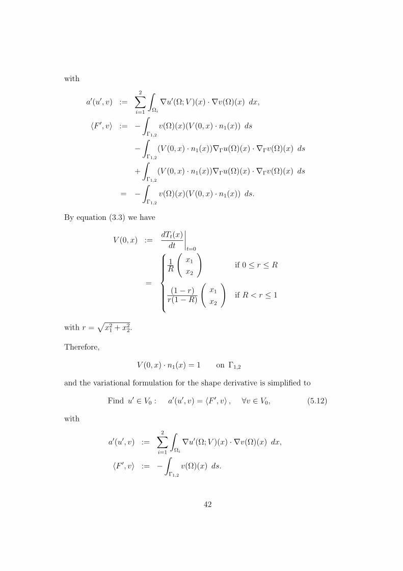
v(Ω)(x)(V (0, x) · n1(x)) ds.
By equation (3.3) we have
V (0, x) :=dTt(x)
dt
∣∣∣∣t=0
=
1R
(x1
x2
)if 0 ≤ r ≤ R
(1− r)r(1−R)
(x1
x2
)if R < r ≤ 1
with r =√
x21 + x2
2.
Therefore,
V (0, x) · n1(x) = 1 on Γ1,2
and the variational formulation for the shape derivative is simplified to
Find u′ ∈ V0 : a′(u′, v) = 〈F ′, v〉 , ∀v ∈ V0, (5.12)
with
a′(u′, v) :=2∑
i=1
∫Ωi
∇u′(Ω; V )(x) · ∇v(Ω)(x) dx,
〈F ′, v〉 := −∫
Γ1,2
v(Ω)(x) ds.
42

The analytical solution of this problem can be computed and is given by:
u′(Ω; V )(x1, x2) =
R ln(R) if 0 ≤ r ≤ R
R ln(r) if R < r ≤ 1(5.13)
with r =√
x21 + x2
2.Note that the shape derivative u′ equals the derivative of u with respect to R,which is reasonable since the radius of subdomain Ω1 is the design parameter.
One can show that for the variational problem (5.12) the assumptions oftheorem 4.1 are satisfied by using trace theorems (cf. [13]) and thereforeuniqueness of the solution is guaranteed.
The cost functionals of consideration were already discussed and they hadthe following form
J(Γ) =1
µ0
∫Γs
∇u(Ω)(x)T Q(x)∇u(Ω)(x) ds
and
J(Γ) =
∫Γs
u2(Ω)(x) ds.
Remark 5.3 As already mentioned, the first functional is only well definedif u is smooth enough, e.g. in H2. This is indeed true for this test problem.
For the test problem we set µ0 = 1 and, since taking the matrix Q(x) as in(4.29) would lead to trivial solutions, Q(x) = I. So the first functional issimplified to
J(Γ) =
∫Γs
∇u(Ω)(x) · ∇u(Ω)(x) ds (5.14)
and for its Eulerian derivative we have
d
dtJ(Γt)
∣∣∣∣t=0
= 2
∫Γs
∇u′(Ω; V )(x) · ∇u(Ω)(x) ds. (5.15)
The first functional will be evaluated at the boundary of some circle withradius re > R, the second functional will be evaluated at the interface Γ1,2.
The Direct Approach
First the solution of the variational problem (5.9) for u is computed. Thenthe solution of the variational problem (5.12) for the shape derivative u′ iscomputed. Now the Eulerian derivative of the functionals (5.15) and (5.3)can be evaluated.
43

The Adjoint Approach for the Second Functional
First the solution of the variational problem (5.9) for u is computed. Thenwe define the adjoint variable λ as solution of the following problem:
Find λ ∈ V0 : a′(λ, w) = 〈G, w〉 , ∀w ∈ V0, (5.16)
with
a′(λ, w) =2∑
i=1
∫Ωi
∇λ(Ω)(x) · ∇w(Ω)(x) dx,
〈G, w〉 := 2
∫Γ1,2
u(Ω)(x)w(Ω)(x) ds.
Since u′ ∈ V0 and (5.16) holds for all functions in V0 we have
d
dtJ(Γt)
∣∣∣∣t=0
= 〈G, u′〉 = a′(λ, u′) = 〈F ′, λ〉 = −∫
Γ1,2
λ(Ω)(x) ds.
The analytical solution of this adjoint problem can be computed and is givenby:
λ(x1, x2) =
−2 ·R(1
4(1−R2) + 1
2R2 ln(R)) ln(R) if 0 ≤ r ≤ R
−2 ·R(14(1−R2) + 1
2R2 ln(R)) ln(r) if R < r ≤ 1
(5.17)
with r =√
x21 + x2
2.
One can show that for the variational problem (5.16) the assumptions oftheorem 4.1 are satisfied by using trace theorems and therefore uniquenessof the solution is guaranteed.
So far we discussed how gradients of functionals can be computed usingthe direct and adjoint method. We saw that the adjoint method is not welldefined for the functional, which describes the torque.Then we considered a particular test problem, applied the direct and adjointmethod there and this resulted in 3 variational problems: the problem for u,the problem for the shape derivative u′ and the adjoint problem for λ. Sofar, everything was formulated in the continuous setting. For solving thesevariational problems, we need to discretize them. This is done by using thefinite element method, which is introduced in the next chapter.
44
Chapter 6
Discretization
The aim of this chapter is to describe the discretization by using the finiteelement method. First we give an introduction to the Galerkin-Ritz methodwith special ansatz functions and then we apply it to our linear problems(the original problem for u, the problem for the shape derivative u′ and theadjoint problem for λ). The resulting systems of linear equations will besolved by the conjugate gradient (CG) method.
6.1 Introduction to the Finite Element Method
A comprehensive introduction to the finite element method (FEM) can befound in [15], [16] and [17].
As starting point we consider a linear variational problem
Find u ∈ V : a(u, v) = 〈F, v〉 , ∀v ∈ V, (6.1)
in a Hilbert space V , whereby a(., .) and 〈F, v〉 should satisfy the assumptionsof the Lax-Milgram theorem (cf. Theorem 4.1), which ensures the existenceand uniqueness of a solution u∗ of the problem (6.1).
The Galerkin-Ritz Method
Let us assume that we have a sequence of finite-dimensional subspacesVh ⊂ V , and we associate the following discrete problems to the variationalproblem (6.1):
Find uh ∈ Vh ⊂ V : a(uh, vh) = 〈F, vh〉 , ∀vh ∈ Vh, (6.2)
where h indicates the discretization parameter and in fact we want to havethat for h→ 0 the solution of the discrete problem u∗h converges to the exact
45
solution u∗. Since Vh ⊂ V , the Lax-Milgram theorem guarantees the exis-tence and uniqueness of a solution u∗h of the discrete problem (6.2).
The next step is to choose appropriate basis functions for the finite-dimensionalspace Vh, such that Vh = spanp(i)(x) : i = 1, ..., Nh, where p(i) denote thebasis functions and Nh the dimension of the space. Since uh ∈ Vh, we canuse the representation
uh(x) =
Nh∑i=1
u(i)h p(i)(x) (6.3)
with the coefficients u(i)h ∈ R. Therefore, we get the Galerkin system
Find uh ∈ RNh : Khuh = fh, (6.4)
with
uh :=(u
(i)h
)Nh
i=1,
Kh :=(a(p(j), p(i))
)Nh
i,j=1,
fh
:=(⟨
F, p(i)⟩)Nh
i=1.
The linear system (6.4) is equivalent to the discrete problem (6.2). Thisequivalence defines the so called Ritz isomorphism:
uh ∈ Vh ←→ uh ∈ RNh . (6.5)
Construction of Vh using the Courant Element
Now we want to construct finite element subspaces of certain Hilbert spacesand corresponding basis functions. First we introduce the notion of triangu-lation:
Definition 6.1 Let Ω ∈ Rd be an open, bounded set with sufficiently smoothboundary. Then Th := δr : r ∈ Rh is called triangulation of Ω if:
1) Ω =⋃
r∈Rh
δr
2) δr ∩ δs = 0.
Additionally we force the triangulation to be admissible, which means in 2D:
46

Definition 6.2 A triangulation Th is admissible if:
δr ∩ δs =
0
common vertex
common edge.
In the Galerkin-Ritz FEM we have to face three main aspects:
• A triangulation Th of the domain Ω.
• The finite element space Vh is constructed such that the functions arecontinuous and for each δr ∈ Th the restriction of vh ∈ Vh is a polyno-mial.
• The basis of Vh is constructed such that the basis functions have localsupport.
In 2D the widely used element is the so called Courant element. The do-main is subdivided into triangles, on which the functions vh should be linear.Therefore we have for the finite element space
Vh := vh ∈ C(Ω)| vh|δr∈ P1 ∀δr ∈ Th. (6.6)
The construction of this space is as follows:
• Let x(j), j ∈ ωh denote all vertices (called nodes) of the triangulationand ωh the index set of the nodes.
• We set
p(i)(x(j)) := δij, ∀i, j ∈ ωh,
with
δij =
1 if i = j
0 otherwise.
This basis is called nodal basis, since the unknowns are the function values atthe nodes: u
(j)h = uh(x
(j)). Therefore the basis function p(i) forms a pyramidfunction with height 1 at the node x(i). Additionally this basis functionshave local support, therefore, since a(p(i), p(j)) = 0 if the supports are notoverlapping, the corresponding stiffness matrix Kh is sparse.
We can write
Vh :=
vh(x) =∑j∈ωh
v(j)p(j)(x)∣∣∣v(j) ∈ R
. (6.7)
with Vh ⊂ H1 for an admissible subdivision into triangles.
47
The Reference Triangle
The stiffness matrix and the load vector (right hand side) are assembled bysumming over the elements δr ∈ Th. The appearing integrals over the ele-ments can be evaluated efficiently using the concept of the reference triangle.For Courant triangles we define the reference triangle as ∆ :=
[ξ1, ξ2] ∈
[0, 1]2∣∣ξ1 + ξ2 ≤ 1
with the following reference basis functions:
p(1)(ξ) := 1− ξ1 − ξ2
p(2)(ξ) := ξ1
p(3)(ξ) := ξ2.
Now every δr can be written as an affine linear transformation of ∆ and,consequently, the basis functions on every δr can be written in terms ofthe reference basis functions. So the integrals can be easily transformedto the reference triangle using the three element nodes x(i,1), x(i,2), x(i,3). Forefficiently evaluating these integrals we used numerical integration (midpointrule).
6.2 The Finite Element Method applied to
the Test Problem
In our test problem we have to solve three variational problems:
• 1) The VP for u:
Find u ∈ V0 = H10 (Ω) : a(u, v) = 〈F, v〉 , ∀v ∈ V0,
with
a(u, v) =2∑
i=1
∫Ωi
∇u(Ω)(x) · ∇v(Ω)(x) dx,
〈F, v〉 =
∫Ω2
v(Ω)(x) dx.
• 2) The VP for u′:
Find u′ ∈ V0 : a′(u′, v) = 〈F ′, v〉 , ∀v ∈ V0,
with
a′(u′, v) =2∑
i=1
∫Ωi
∇u′(Ω; V )(x) · ∇v(Ω)(x) dx,
〈F ′, v〉 = −∫
Γ1,2
v(Ω)(x) ds.
48

• 3) The VP for λ:
Find λ ∈ V0 : a′(λ, w) = 〈G, w〉 , ∀w ∈ V0,
with
a′(λ, w) =2∑
i=1
∫Ωi
∇λ(Ω)(x) · ∇w(Ω)(x) dx,
〈G, w〉 = 2
∫Γ1,2
u(Ω)(x)w(Ω)(x) ds.
In all the problems we have the same Hilbert space H10 and the same bilinear
form a(u, v). One can easily see that
V0h :=
vh(x) =∑j∈ωh
v(j)p(j)(x)∣∣∣v(j) ∈ R
⊂ H1
0
where ωh is the set of all indices whose corresponding nodes do not lie on Γ.
The construction of Kh starts with initializing all the entries with 0. Thenwe have
Kh(i,j) = a(p(j), p(i)) =
∫Ω
∇p(j) · ∇p(i)(x) dx =∑
r∈Bi,j
∫δr
∇p(j) · ∇p(i)(x) dx
where Bi,j := Bi ∩Bj and Bi := r ∈ Rh : x(i) ∈ δr.Therefore we iterate over all elements δr, compute the integrals using thereference triangle in each step and add this value to Kh(i,j).Because of the Ritz isomorphism the properties of the bilinear form carryover to the stiffness matrix and therefore the stiffness matrix in the threeproblems is symmetric and positive definite.
For calculating the load vectors, the same principle is used.
The implementation of the interface conditions works through iterating overall edges, which belong to the interface. As a reference element the line from0 to 1 is taken. The rest is almost the same as above.
The implementation of the homogeneous Dirichlet boundary condition worksas follows:
• set u(j)h = 0 for j ∈ γh with ωh = ωh ∪ γh
• set Kh(i,j) = Kh(j,i) = δij
• set f(j)h = 0 for j ∈ γh.
49

6.3 The CG - Method
If the matrix K in the linear system
Ku = f, (6.8)
is symmetric and positive definite, problem (6.8) is equivalent to the followingminimization problem:
J(u) :=1
2(Ku, u)− (f, u)→ min
u, (6.9)
because
∇J(u) = Ku− f!= 0,
∇2J(u) = K = KT > 0.
J is called the energy functional.
The CG - algorithm reads as follows:
• Initialization: choose initial guess u0
d0 = f −Ku0
p0 = d0
• Iteration: for n = 0, 1, 2, ... until convergence do
un+1 = un + α(n)pn with α(n) =(dn, pn)
(Kpn, pn),
dn+1 = dn − α(n)Kpn,
pn+1 = dn+1 − β(n)pn with β(n) =(dn+1, Kpn)
(Kpn, pn).
end.
For the CG - method we have the following convergence result:
Theorem 6.3 Let K ∈ Rn×n be symmetric and positive definite.Then the CG - method is convergent and the following error estimate holds:
||un − u||K ≤2qn
1 + q2n||u0 − u||K ≤ 2qn||u0 − u||K , (6.10)
with
0 ≤ q =
√κ(K)− 1√κ(K) + 1
< 1, (6.11)
where κ(K) is the condition number of the matrix K.
50

Since the stiffness matrix in our three problems satisfies these assumptions,the CG - method can be used for solving them.In the next chapter the numerical results are presented.
51
Chapter 7
Numerical Results
In this chapter the numerical results for the direct and adjoint method appliedto the test problem from chapter 5 are presented. As already mentioned, forcomparing the two approaches we use the functional (5.2), since the adjointmethod is not well defined for the functional (5.14). But we also present theresults of the direct method used with the functional (5.14).
For the following results the radius of subdomain Ω1 was set to R = 0.4.
7.1 The Analytical Solutions
The analytical solutions of (5.9), (5.12) and (5.16) are:
u(x1, x2) =
14(1− 0.42) + 1
20.42 ln(0.4) ≈ 0.137 if 0 ≤ r ≤ R
14(1− r2) + 1
20.42 ln(r) if R < r ≤ 1,
u′(Ω; V )(x1, x2) =
0.4 ln(0.4) ≈ −0.367 if 0 ≤ r ≤ R
0.4 ln(r) if R < r ≤ 1
and
λ(x1, x2) =
−2 · 0.4(1
4(1− 0.42) + 1
20.42 ln(0.4)) ln(0.4) ≈ 0.1002 if 0 ≤ r ≤ R
−2 · 0.4(14(1− 0.42) + 1
20.42 ln(0.4)) ln(r) if R < r ≤ 1
with r =√
x21 + x2
2.
52
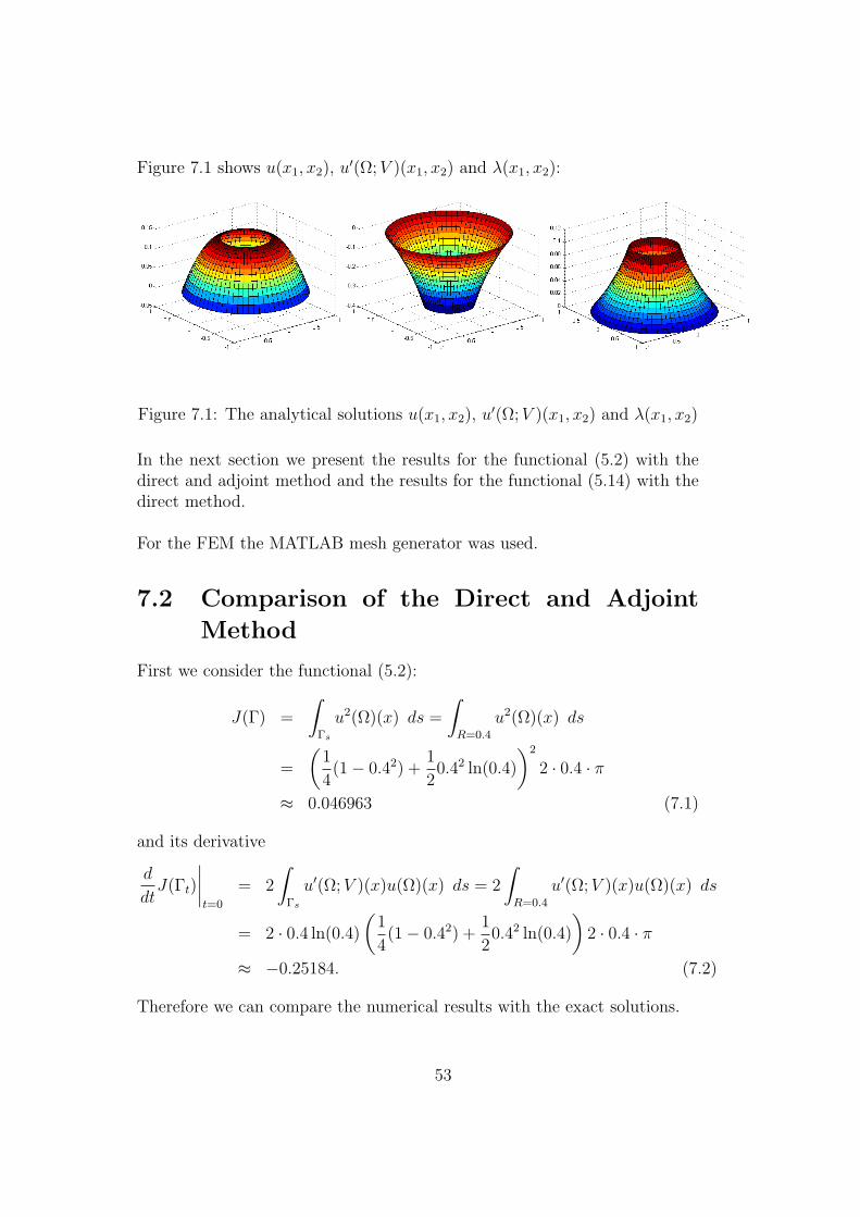
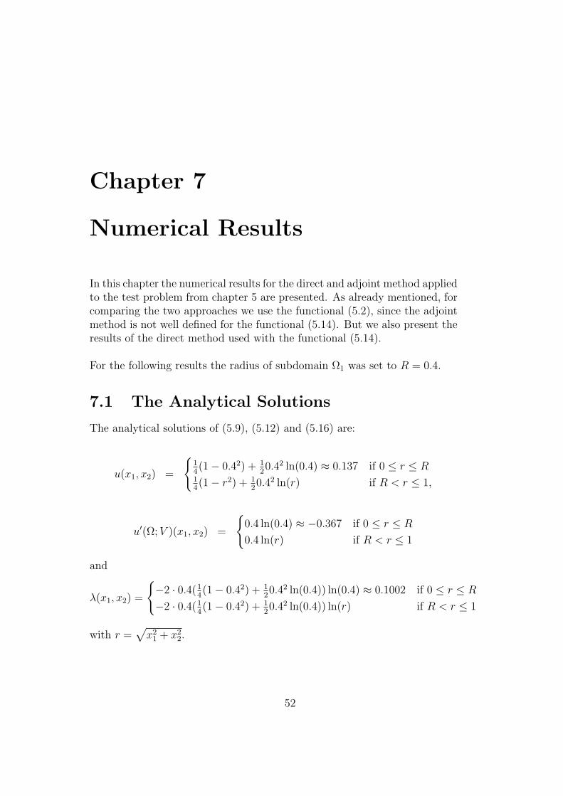
Figure 7.1 shows u(x1, x2), u′(Ω; V )(x1, x2) and λ(x1, x2):
Figure 7.1: The analytical solutions u(x1, x2), u′(Ω; V )(x1, x2) and λ(x1, x2)
In the next section we present the results for the functional (5.2) with thedirect and adjoint method and the results for the functional (5.14) with thedirect method.
For the FEM the MATLAB mesh generator was used.
7.2 Comparison of the Direct and Adjoint
Method
First we consider the functional (5.2):
J(Γ) =
∫Γs
u2(Ω)(x) ds =
∫R=0.4
u2(Ω)(x) ds
=
(1
4(1− 0.42) +
1
20.42 ln(0.4)
)2
2 · 0.4 · π
≈ 0.046963 (7.1)
and its derivative
d
dtJ(Γt)
∣∣∣∣t=0
= 2
∫Γs
u′(Ω; V )(x)u(Ω)(x) ds = 2
∫R=0.4
u′(Ω; V )(x)u(Ω)(x) ds
= 2 · 0.4 ln(0.4)
(1
4(1− 0.42) +
1
20.42 ln(0.4)
)2 · 0.4 · π
≈ −0.25184. (7.2)
Therefore we can compare the numerical results with the exact solutions.
53

For the FEM we used the following meshes:
mesh number number of unknowns (nodes) number of triangles1 152 2682 571 10723 2213 42884 8713 171525 34577 68608
The meshes were generated using the ”Refinement” - option in Matlab.
In figure 7.2 one can see the generated meshes. Figures 7.3 - 7.7 show theFE solutions of the problems (5.9), (5.12) and (5.16) for u, u′ and λ.
54
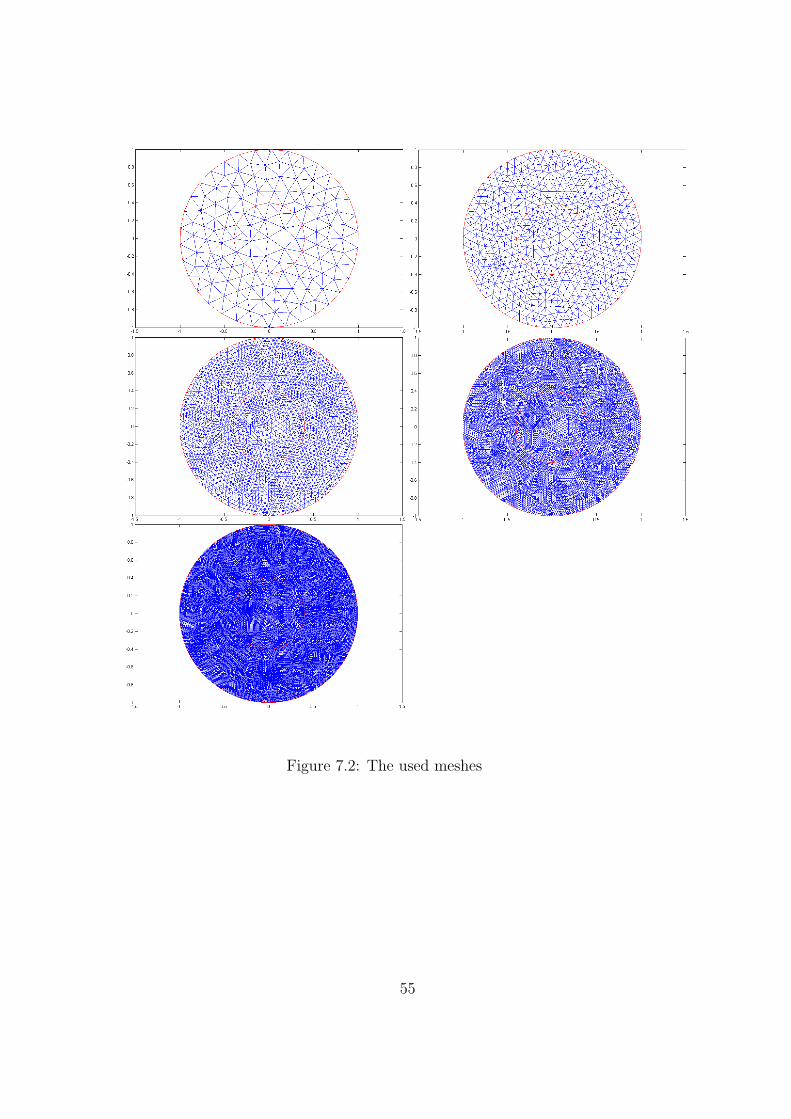
Figure 7.2: The used meshes
55
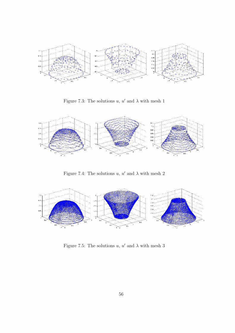
Figure 7.3: The solutions u, u′ and λ with mesh 1
Figure 7.4: The solutions u, u′ and λ with mesh 2
Figure 7.5: The solutions u, u′ and λ with mesh 3
56
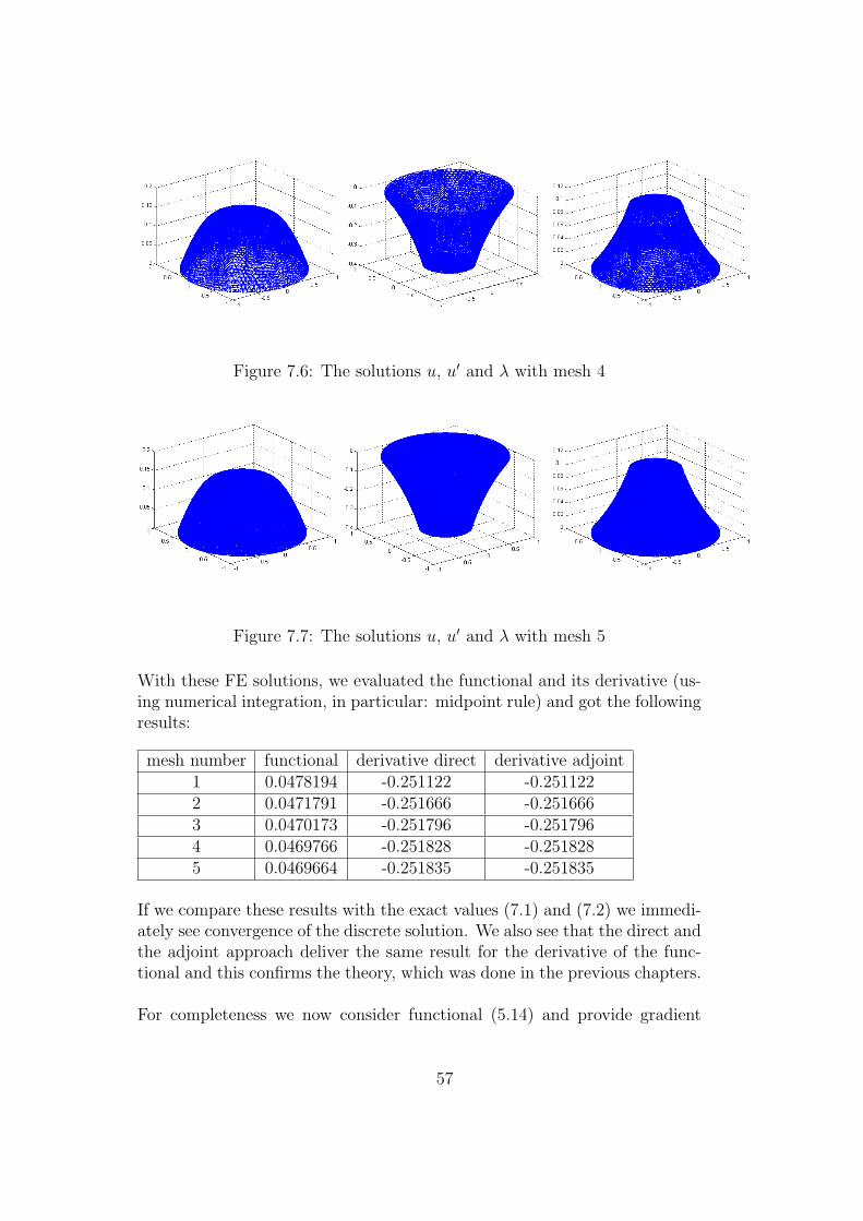
Figure 7.6: The solutions u, u′ and λ with mesh 4
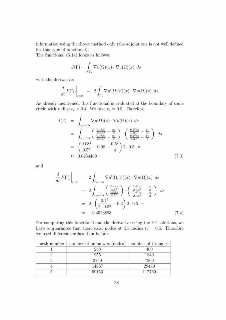
Figure 7.7: The solutions u, u′ and λ with mesh 5
With these FE solutions, we evaluated the functional and its derivative (us-ing numerical integration, in particular: midpoint rule) and got the followingresults:
mesh number functional derivative direct derivative adjoint1 0.0478194 -0.251122 -0.2511222 0.0471791 -0.251666 -0.2516663 0.0470173 -0.251796 -0.2517964 0.0469766 -0.251828 -0.2518285 0.0469664 -0.251835 -0.251835
If we compare these results with the exact values (7.1) and (7.2) we immedi-ately see convergence of the discrete solution. We also see that the direct andthe adjoint approach deliver the same result for the derivative of the func-tional and this confirms the theory, which was done in the previous chapters.
For completeness we now consider functional (5.14) and provide gradient
57
information using the direct method only (the adjoint one is not well definedfor this type of functional).The functional (5.14) looks as follows:
J(Γ) =
∫Γs
∇u(Ω)(x) · ∇u(Ω)(x) ds
with the derivative:
d
dtJ(Γt)
∣∣∣∣t=0
= 2
∫Γs
∇u′(Ω; V )(x) · ∇u(Ω)(x) ds.
As already mentioned, this functional is evaluated at the boundary of somecircle with radius re > 0.4. We take re = 0.5. Therefore,
J(Γ) =
∫re=0.5
∇u(Ω)(x) · ∇u(Ω)(x) ds
=
∫re=0.5
(0.42x1
2·0.52 − x1
20.42x2
2·0.52 − x2
2
)·(
0.42x1
2·0.52 − x1
20.42x2
2·0.52 − x2
2
)ds
=
(0.082
0.52− 0.08 +
0.52
4
)2 · 0.5 · π
≈ 0.0254469 (7.3)
and
d
dtJ(Γt)
∣∣∣∣t=0
= 2
∫re=0.5
∇u′(Ω; V )(x) · ∇u(Ω)(x) ds
= 2
∫re=0.5
(0.4x1
0.52
0.4x2
0.52
)·(
0.42x1
2·0.52 − x1
20.42x2
2·0.52 − x2
2
)ds
= 2 ·(
0.43
2 · 0.52− 0.2
)2 · 0.5 · π
≈ −0.4523893. (7.4)
For computing this functional and the derivative using the FE solutions, wehave to guarantee that there exist nodes at the radius re = 0.5. Thereforewe used different meshes than before:
mesh number number of unknowns (nodes) number of triangles1 248 4602 955 18403 3749 73604 14857 294405 59153 117760
58

In figure 7.8 one can see the generated meshes.
Figure 7.8: The used meshes
For evaluating the functional and the derivative, we need to calculate gradi-ents out of the FE solutions. Since we used P1-functions for the FEM, thegradient is constant on each finite element, and therefore will not be contin-uous across the edge of two neighbouring elements. This means that we havethe following possibilities:
59

• use the information about the gradient in elements which touch thecircle with radius re = 0.5 inside
• use the information about the gradient in elements which touch thecircle with radius re = 0.5 outside
• take a mean value of the inside and outside gradient information.
How this is meant is illustrated in figure 7.9
Figure 7.9: The touching elements
The blue triangles are the elements which touch the circle with radiusre = 0.5 inside and the red ones are the elements which the touch this circleoutside. For the calculation of the gradient of the FE solution according tothe first possibility, only the blue triangles are used. For the calculation ofthe gradient of the FE solution according to the second possibility, only thered triangles are used. For the calculation of the gradient of the FE solutionaccording to the third possibility, the gradient is calculated in the red andblue triangles and then a mean value of the gradient of the neighbouring redand blue triangles is taken.
60

For the different possibilities we got the following results:
• gradient inside
mesh number functional derivative1 0.00849013 -0.2901042 0.0156795 -0.3755723 0.0202496 -0.4152434 0.0227719 -0.4341465 0.0240905 -0.443351
• gradient outside
mesh number functional derivative1 0.048333 -0.5525962 0.036016 -0.5075363 0.0304912 -0.4811644 0.0279072 -0.4670685 0.0266615 -0.459801
• mean value of gradient inside and outside
mesh number functional derivative1 0.0242782 -0.4424112 0.0247937 -0.4468633 0.0251064 -0.4495264 0.0252736 -0.4509365 0.0253595 -0.451658
If we compare these results with the exact values (7.3) and (7.4) we see, thatthe solutions in all cases converge. But we also see that the one with themean values is the fastest converging solution.
For interest, consider the adjoint problem with this type of functional:
Find λ ∈ V0 = H10 (Ω) : a′(λ, w) = 〈G, w〉 , ∀w ∈ V0,
with
a′(λ, w) =2∑
i=1
∫Ωi
∇λ(Ω)(x) · ∇w(Ω)(x) dx,
〈G, w〉 = 2
∫Γs
∇u(Ω)(x) · ∇w(Ω)(x) ds.
61
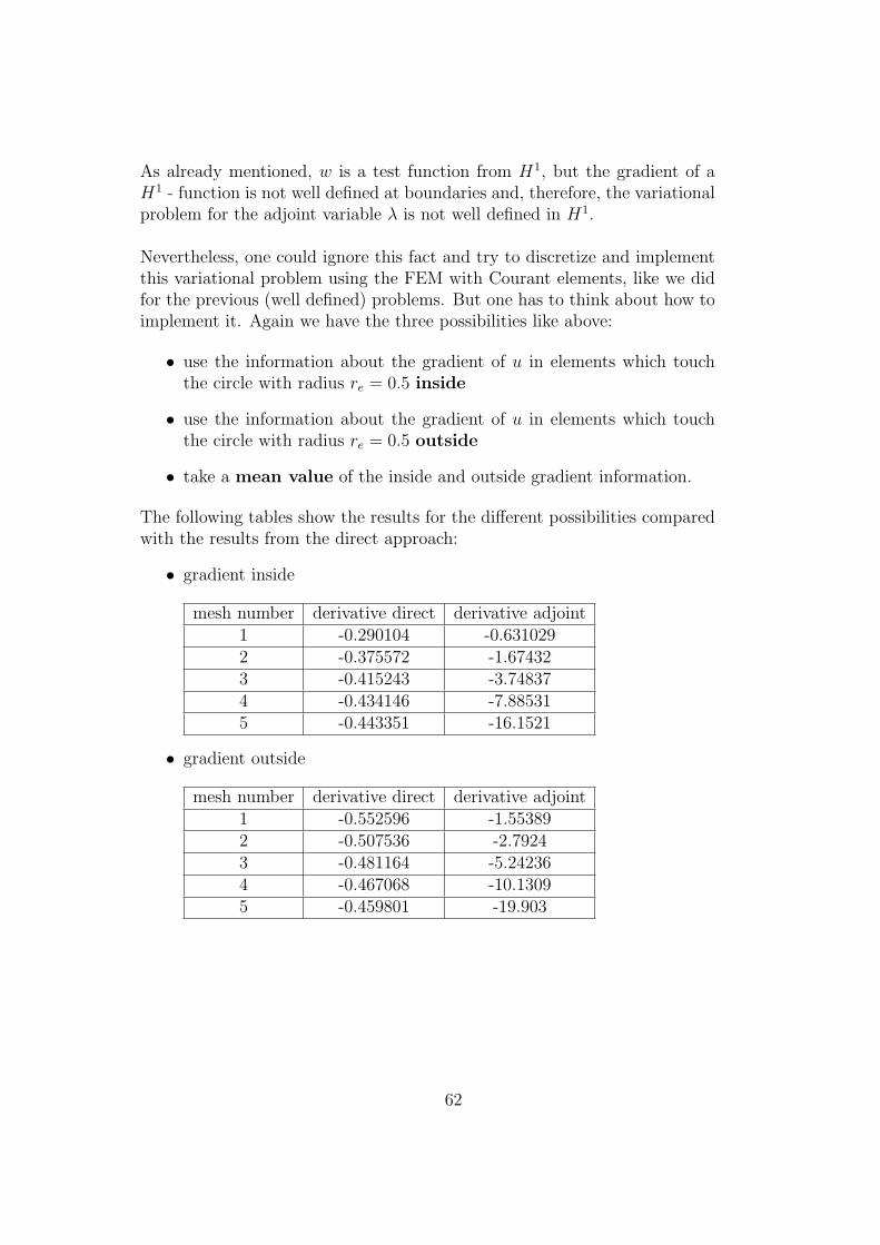
As already mentioned, w is a test function from H1, but the gradient of aH1 - function is not well defined at boundaries and, therefore, the variationalproblem for the adjoint variable λ is not well defined in H1.
Nevertheless, one could ignore this fact and try to discretize and implementthis variational problem using the FEM with Courant elements, like we didfor the previous (well defined) problems. But one has to think about how toimplement it. Again we have the three possibilities like above:
• use the information about the gradient of u in elements which touchthe circle with radius re = 0.5 inside
• use the information about the gradient of u in elements which touchthe circle with radius re = 0.5 outside
• take a mean value of the inside and outside gradient information.
The following tables show the results for the different possibilities comparedwith the results from the direct approach:
• gradient inside
mesh number derivative direct derivative adjoint1 -0.290104 -0.6310292 -0.375572 -1.674323 -0.415243 -3.748374 -0.434146 -7.885315 -0.443351 -16.1521
• gradient outside
mesh number derivative direct derivative adjoint1 -0.552596 -1.553892 -0.507536 -2.79243 -0.481164 -5.242364 -0.467068 -10.13095 -0.459801 -19.903
62
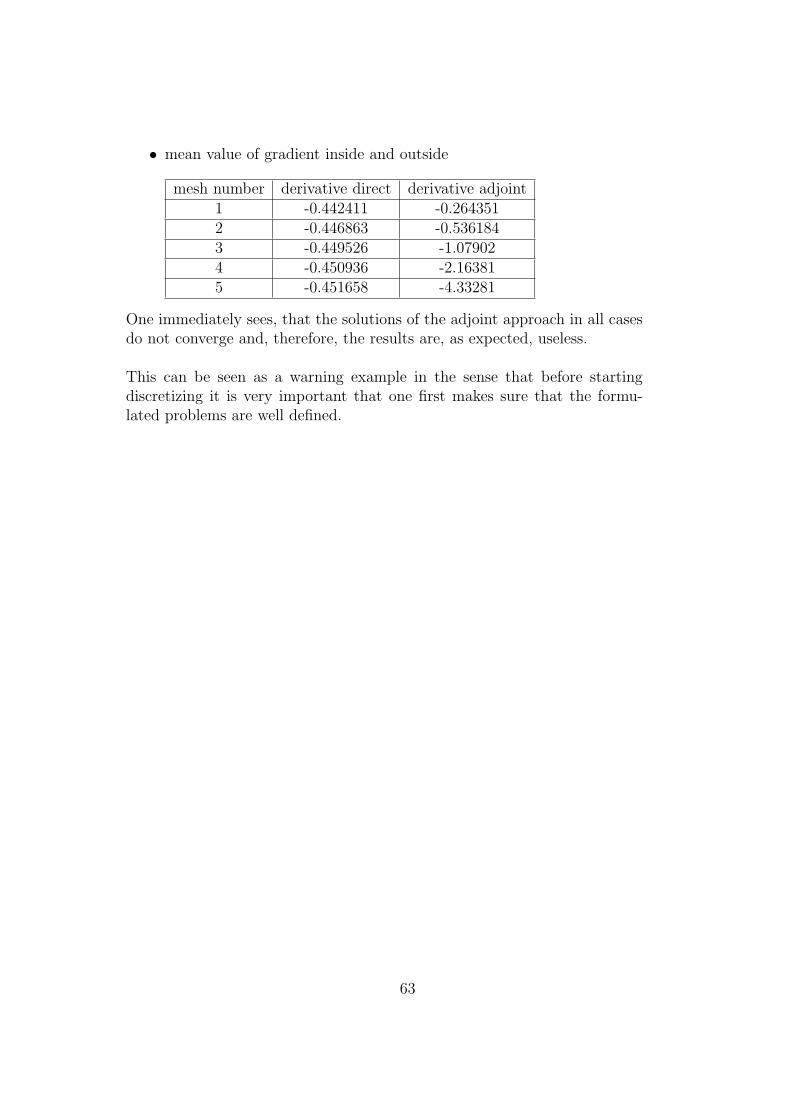
• mean value of gradient inside and outside
mesh number derivative direct derivative adjoint1 -0.442411 -0.2643512 -0.446863 -0.5361843 -0.449526 -1.079024 -0.450936 -2.163815 -0.451658 -4.33281
One immediately sees, that the solutions of the adjoint approach in all casesdo not converge and, therefore, the results are, as expected, useless.
This can be seen as a warning example in the sense that before startingdiscretizing it is very important that one first makes sure that the formu-lated problems are well defined.
63
Chapter 8
Conclusions and Outlook
8.1 Conclusion
In this thesis the entire mathematical treatment of using the shape derivativeapproach in shape optimization is embraced. We introduced two differentmethods for providing gradient information of functionals, which consist ofdomain and/or boundary integrals and depend on the solution of some stateproblem: the direct and the adjoint technique. We have seen that the adjointapproach has a great advantage compared to the direct one: the adjoint stateequation has to be solved only once.We considered a magnetostatic problem, where we have derived a mathemat-ical formulation from the governing physical equations (Maxwell). Then weapplied the two approaches and this resulted in three linear variational prob-lems. Solvability of the problems has been proven under the assumptions ofthe Lax-Milgram theorem.
We have discretized the continuous problems with the finite element method.In order to solve the resulting systems of equations, where the involved ma-trices are symmetric and positive definite, we used the conjugate gradientmethod.
Numerical results have shown that indeed the direct and the adjoint ap-proach lead to the same results for the test problem. But we also have seenthat there exist examples where the adjoint technique is not useful in thesense of providing suitable results.
8.2 Outlook
This work can be continued in the following directions:
64

• The nonlinear problem:
When deriving the mathematical formulation we assumed the involvedmaterials to be linear and therefore the variational problem got linear.But in most of the problems in physics there is a nonlinear part in-volved. Therefore the adjoint method has to be set up in the nonlinearcase.
• The adjoint method for ”general” functionals:
We have shown an example of a functional where the adjoint problem,which was derived in the usual way (straight forward), is not well de-fined and therefore the adjoint approach is inapplicable in the sense weintroduced it. For this one has to think about how to reformulate theadjoint problem.
65

Bibliography
[1] J.HASLINGER and R.A.E.MAKINEN. Introduction to Shape Optimiza-tion: Theory, Approximation and Computation. SIAM, 2003.
[2] JAN SOKOLOWSKI and JEAN-P. ZOLESIO. Introduction to ShapeOptimization: Shape sensitivity analysis. Springer Verlag Berlin, 1992.
[3] JEAN-P. ZOLESIO and M.C. DELFOUR. Shapes and Geometries:Analysis, Differential Calculus and Optimization. SIAM, 2001.
[4] P.LE TALLEC and E.LAPORTE. Numerical Methods in Sensitivity andShape Optimization. BIRKHAUSER, 2002.
[5] W.MUHLHUBER. Spezialforschungsbereich F013: Various Aspects ofShape Optimization. Johannes Kepler University Linz, Presentation.
[6] E.J.HAUG K.K.CHOI and V.KOMKOV. Mathematics in Science andEngineering, Volume 177: Design Sensitivity Analysis of Structural Sys-tems. ACADEMIC PRESS, INC, 1986.
[7] H.ENGL. Lecture Notes for the Course Mathematical Methods in Con-tinuum Mechanics. Johannes Kepler University Linz, Winter Semester2008/09.
[8] W.ZULEHNER. Lecture Notes for the Course Numerical Methodsin Continuum Mechanics. Johannes Kepler University Linz, SummerSemester 2009.
[9] B.HEISE. Mehrgitter-Newton-Verfahren zur Berechnung nichtlinearermagnetischer Felder. Technische Universitat Chemnitz, 1991.
[10] S.MUHLBOCK and A.LECHNER. Numerical solution of nonlinear sta-tionary magnetic field problems. Johannes Kepler University Linz, Bach-elor Thesis, 2008.
[11] C.PECHSTEIN. Multigrid-Newton-Methods for Nonlinear Magneto-static Problems. Johannes Kepler University Linz, Master Thesis, 2004.
66

[12] W.GRUBER W.AMRHEIN S.SILBER H.GRABNER andM.REISINGER. Theoretical analysis of force and torque calcula-tion in magnetic bearing systems with circular airgap. Institute ofElectrical Drives and Power Electronics JKU Linz.
[13] R.ADAMS. Sobolev Spaces. Academic Press, New York, 1975.
[14] U.LANGER. Lecture Notes for the Course Numerical Methods for Par-tial Differential Equations. Johannes Kepler University Linz, WinterSemester 2007/08.
[15] P.G. CIARLET. The Finite Element Method for Elliptic Problems. Clas-sics in Applied Mathematics, Vol. 40, SIAM, Philadelphia, 2002.
[16] U.LANGER and M.JUNG. Methode der finiten Elemente fur Inge-nieure. Teubner-Verlag, Stuttgart, Leipzig, Wiesbaden, 2001.
[17] W.ZULEHNER. Lecture Notes for the Course Numerical Methods forElliptic Problems. Johannes Kepler University Linz, Summer Semester2008.
67
Eidesstattliche Erklarung
Ich, Markus Kollmann, erklare an Eides statt, dass ich die vorliegende Mas-terarbeit selbststandig und ohne fremde Hilfe verfasst, andere als die angegebe-nen Quellen und Hilfsmittel nicht benutzt bzw. die wortlich oder sinngemaßentnommenen Stellen als solche kenntlich gemacht habe.
Leonding, Februar 2010 Markus Kollmann
68

Curriculum Vitae
Name: Markus Kollmann
Nationality: Austria
Date of Birth: 1st of October, 1984
Place of Birth: Linz, Austria
Education:1991 - 1995 Elementary School
Keferfeld, Linz1995 - 1999 Secondary Comprehensive School
Landwiedstraße, Linz1999 - 2004 Polytechnic
Leonding2005 - 2008 Studies of Technical Mathematics (Bachelor)
Johannes Kepler University, Linz2008 - 2010 Studies of Industrial Mathematics (Master)
Johannes Kepler University, Linz
Special Activities:August 2009 23rd ECMI Modelling Week, Wroclaw, Poland
69