CSUG/SPE 149471

Recovery Factor and Reserves Estimation in the Bakken Petroleum System (Analysis of the Antelope, Sanish and Parshall fields) P. Dechongkit and M. Prasad, Colorado School of Mines

Copyright 2011, Society of Petroleum Engineers This paper was prepared for presentation at the Canadian Unconventional Resources Conference held in Calgary, Alberta, Canada, 15–17 November 2011. This paper was selected for presentation by a CSUG/SPE program committee following review of information contained in an abstract submitted by the author(s). Contents of the paper have not been reviewed by the Society of Petroleum Engineers and are subject to correction by the author(s). The material does not necessarily reflect any position of the Society of Petroleum Engineers, its officers, or members. Electronic reproduction, distribution, or storage of any part of this paper without the written consent of the Society of Petroleum Engineers is prohibited. Permission to reproduce in print is restricted to an abstract of not more than 300 words; illustrations may not be copied. The abstract must contain conspicuous acknowledgment of SPE copyright.

Abstract Recovery factor (RF) is one of the most important parameters for economic justification in the petroleum industry. The RF is calculated from the ratio between expected ultimate recovery (EUR) and original oil-in-place (OOIP). However, many uncertainties exist in OOIP estimations, mainly due to inaccurate information about reservoir drainage area. In unconventional reservoirs, the estimations of drainage area and OOIP are more complicated due to unknown factors such as fracture networks in the system, reservoir pressures, pore volumes, and in situ hydrocarbon properties.

We analyze here a case study of the Bakken Formation where the RF is still unclear and not frequently reported. RF for the Bakken formation from previous studies ranged from 0.7 – 50% (Price, 1984; Bohrer et al., 2008) derived from different approaches. In this paper, we use the material balance equation (MBE) approach to determine the deterministic (single value) and probabilistic (distribution) RF values in the Bakken Formation (the Antelope, Sanish and Parshall fields). We also perform a sensitivity analysis for the input parameters in our MBE approach.From the actual well production data, the EUR can be estimated from decline curve analysis (DCA) with knowledge of abandonment rate data. The DCA technique based on history data is used as forecast model for predicting the EUR and remaining volume. Once the RF and EUR are calculated, the OOIP value can be evaluated as the ratio between EUR and RF.

In the studied fields, RF result of the Parshall Field is highest because the produced gas-oil ratio is lower than the other two fields. From the EUR results, the high EUR area in the Antelope Field is located in the center of the field. For the Sanish and Parshall fields, high EUR areas are located in the east and west side, respectively. In addition, it appears that EUR has a direct relationship to the hydrocarbon pore volume per area (HCPV/area) distribution. For each field, the results of OOIP per well from the ratio between EUR and RF are presented, and these data can be compared with the volumetric OOIP for proper well spacing plan of future projects. Introduction Many unconventional formations have large volumes of remaining oil still contained in the reservoir. Recovery Factor (RF) is such formations is difficult to assess mainly because the input data needed for calculations are poorly known and can have large uncertainties. Moreover, less production data in young fields cause uncertainties in estimations as well. For example, RF for the Bakken Formation from previous studies ranged from 0.7 – 50% (Price, 1984; Bohrer et al., 2008). We investigate here the Bakken Formation and analyze distributions of the RF given a possible range of the input parameters. We also analyze the effects of each of the input parameters on our calculations to determine RF sensitivity to different input values.

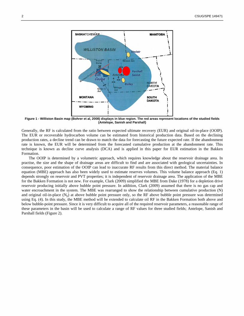
The Bakken Formation is a thin and deep unit from the Late Devonain to Early Mississippian (Meissner, 1978) covering 200,000 square miles (Houston et al., 2010) in the Williston Basin (Figure 1). The Williston Basin has large volumes of remaining oil still contained in the reservoir. The recovery of this remaining oil is related to the recovery factor (RF), thus affecting the expected net revenue of projects into the Bakken.

In unconventional reservoirs, such as tight sands or shale reservoirs, multi-stage hydraulic fracturing is required to make the reservoir productive. In such formations, the RF calculation is more complicated due to the complexity of reservoir drainage area estimation. The drainage area depends on boundaries and spatial distributions of naturally and hydraulically fractured networks, which are very difficult to determine. Thus, the RF result from the direct method contains many uncertainties. For example, in the Bakken Formation, the current recovery factor is still ambiguous and not often reported. In 1992, the RF was estimated between 15% to 20% for horizontal wells (Reisz, 1992). In 2008, from reserves and RF analyses by county, RF was proposed to range from 0.7% to 3.7% (Bohrer et al., 2008). In 2009, the factor was recently estimated at approximately 6.1% to 8.7% (Clark, 2009).

2 CSUG/SPE 149471

Figure 1 - Williston Basin map (Bohrer et al, 2008) displays in blue region. The red areas represent locations of the studied fields

(Antelope, Sanish and Parshall)

Generally, the RF is calculated from the ratio between expected ultimate recovery (EUR) and original oil-in-place (OOIP). The EUR or recoverable hydrocarbon volume can be estimated from historical production data. Based on the declining production rates, a decline trend can be drawn to match the data for forecasting the future expected rate. If the abandonment rate is known, the EUR will be determined from the forecasted cumulative production at the abandonment rate. This technique is known as decline curve analysis (DCA) and is applied in this paper for EUR estimation in the Bakken Formation.

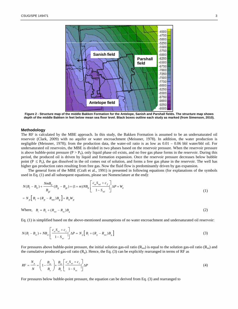
The OOIP is determined by a volumetric approach, which requires knowledge about the reservoir drainage area. In practise, the size and the shape of drainage areas are difficult to find and are associated with geological uncertainties. In consequence, poor estimation of the OOIP can lead to inaccurate RF results from this direct method. The material balance equation (MBE) approach has also been widely used to estimate reserves volumes. This volume balance approach (Eq. 1) depends strongly on reservoir and PVT properties; it is independent of reservoir drainage area. The application of the MBE for the Bakken Formation is not new. For example, Clark (2009) simplified the MBE from Dake (1978) for a depletion drive reservoir producing initially above bubble point pressure. In addition, Clark (2009) assumed that there is no gas cap and water encroachment in the system. The MBE was rearranged to show the relationship between cumulative production (N) and original oil-in-place (Np) at above bubble point pressure only, so the RF above bubble point pressure was determined using Eq. (4). In this study, the MBE method will be extended to calculate oil RF in the Bakken Formation both above and below bubble-point pressure. Since it is very difficult to acquire all of the required reservoir parameters, a reasonable range of these parameters in the basin will be used to calculate a range of RF values for three studied fields; Antelope, Sanish and Parshall fields (Figure 2).

Antelope

CSUG/SPE 149471 3

Figure 2 - Structure map of the middle Bakken Formation for the Antelope, Sanish and Parshall fields. The structure map shows depth of the middle Bakken in feet below mean sea floor level. Black boxes outline each study as marked (from Simenson, 2010).

Methodology The RF is calculated by the MBE approach. In this study, the Bakken Formation is assumed to be an undersaturated oil reservoir (Clark, 2009) with no aquifer or water encroachment (Meissner, 1978). In addition, the water production is negligible (Meissner, 1978); from the production data, the water-oil ratio is as low as 0.01 – 0.06 bbl water/bbl oil. For undersaturated oil reservoirs, the MBE is divided in two phases based on the reservoir pressure. When the reservoir pressure is above bubble-point pressure (P > Pb), only liquid phase oil exists, and no free gas phase forms in the reservoir. During this period, the produced oil is driven by liquid and formation expansion. Once the reservoir pressure decreases below bubble point (P ≤ Pb), the gas dissolved in the oil comes out of solution, and forms a free gas phase in the reservoir. The well has higher gas production rates resulting from free gas. Now the fluid flow is predominantly driven by gas expansion.

The general form of the MBE (Craft et al., 1991) is presented in following equations (for explanations of the symbols used in Eq. (1) and all subsequent equations, please see Nomenclature at the end):

[ ]

( ) ( ) (1 )1

( )

w wi ftit ti g gi ti e

gi wi

p t p soi g w p

c S cNmBN B B B B m NB P W

B S

N B R R B B W

+− + − + + Δ +

−

= + − +

⎡ ⎤⎢ ⎥⎣ ⎦ (1)

Where, ( )t o soi so gB B R R B= + − (2)

Eq. (1) is simplified based on the above-mentioned assumptions of no water encroachment and undersaturated oil reservoir:

[ ]( ) ( )1

w wi ft oi oi p t p soi g

wi

c S cN B B NB P N B R R B

S

+− + Δ = + −

−

⎡ ⎤⎢ ⎥⎣ ⎦

(3)

For pressures above bubble-point pressure, the initial solution gas-oil ratio (Rsoi) is equal to the solution gas-oil ratio (Rso) and the cumulative produced gas-oil ratio (Rp). Hence, the Eq. (3) can be explicitly rearranged in terms of RF as

11

p w wi foi oi

o o wi

N c S cB BRF P

N B B S

+= = − + Δ

−

⎛ ⎞ ⎡ ⎤⎜ ⎟ ⎢ ⎥⎝ ⎠ ⎣ ⎦

(4)

For pressures below bubble-point pressure, the equation can be derived from Eq. (3) and rearranged to

Sanish field

Antelope field

Parshall field

4 CSUG/SPE 149471

[ ]

( )1

( )

w wi ft oi oi

p wi

t p soi g

c S cB B B P

N SRF

N B R R B

+− + Δ

−= =

+ −

⎡ ⎤⎢ ⎥⎣ ⎦ (5)

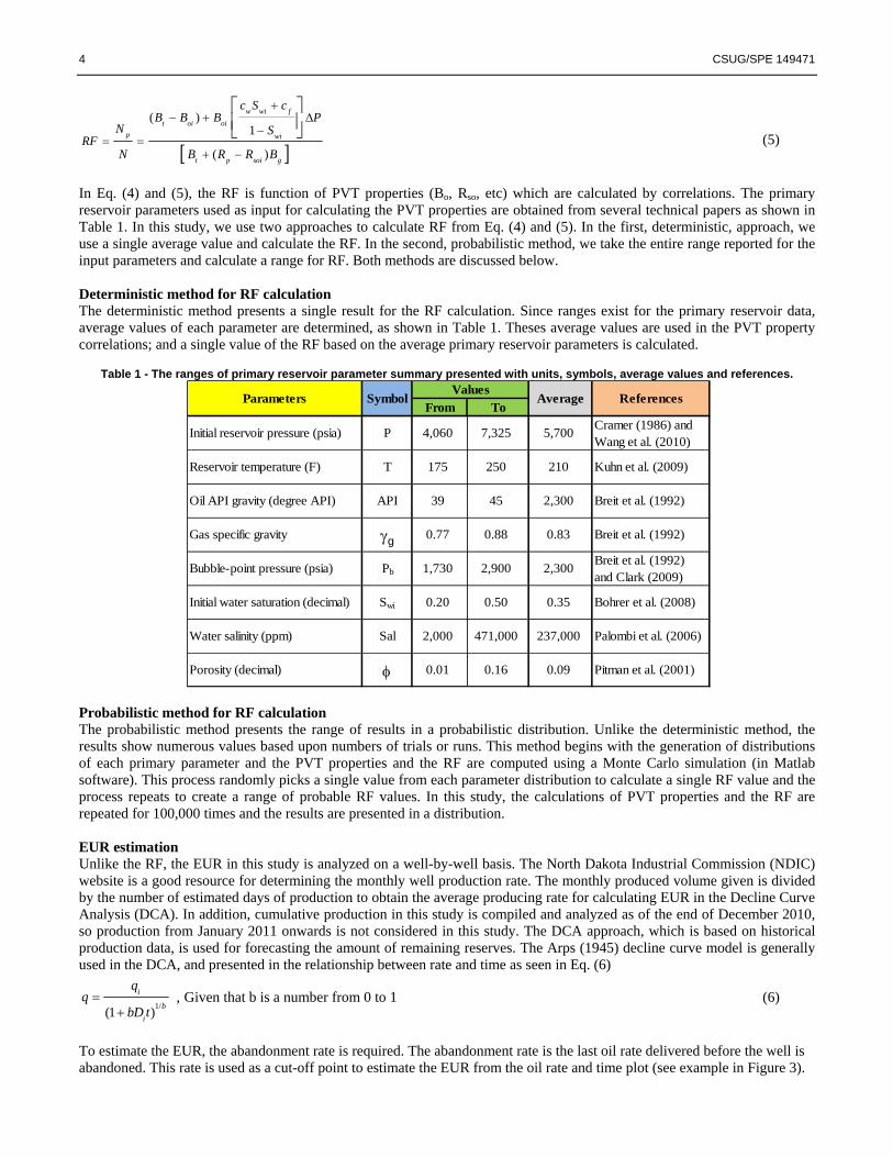
In Eq. (4) and (5), the RF is function of PVT properties (Bo, Rso, etc) which are calculated by correlations. The primary reservoir parameters used as input for calculating the PVT properties are obtained from several technical papers as shown in Table 1. In this study, we use two approaches to calculate RF from Eq. (4) and (5). In the first, deterministic, approach, we use a single average value and calculate the RF. In the second, probabilistic method, we take the entire range reported for the input parameters and calculate a range for RF. Both methods are discussed below. Deterministic method for RF calculation The deterministic method presents a single result for the RF calculation. Since ranges exist for the primary reservoir data, average values of each parameter are determined, as shown in Table 1. Theses average values are used in the PVT property correlations; and a single value of the RF based on the average primary reservoir parameters is calculated.

Table 1 - The ranges of primary reservoir parameter summary presented with units, symbols, average values and references.

Probabilistic method for RF calculation The probabilistic method presents the range of results in a probabilistic distribution. Unlike the deterministic method, the results show numerous values based upon numbers of trials or runs. This method begins with the generation of distributions of each primary parameter and the PVT properties and the RF are computed using a Monte Carlo simulation (in Matlab software). This process randomly picks a single value from each parameter distribution to calculate a single RF value and the process repeats to create a range of probable RF values. In this study, the calculations of PVT properties and the RF are repeated for 100,000 times and the results are presented in a distribution. EUR estimation Unlike the RF, the EUR in this study is analyzed on a well-by-well basis. The North Dakota Industrial Commission (NDIC) website is a good resource for determining the monthly well production rate. The monthly produced volume given is divided by the number of estimated days of production to obtain the average producing rate for calculating EUR in the Decline Curve Analysis (DCA). In addition, cumulative production in this study is compiled and analyzed as of the end of December 2010, so production from January 2011 onwards is not considered in this study. The DCA approach, which is based on historical production data, is used for forecasting the amount of remaining reserves. The Arps (1945) decline curve model is generally used in the DCA, and presented in the relationship between rate and time as seen in Eq. (6)

1/(1 )

i

bi

qq

bD t=

+ , Given that b is a number from 0 to 1 (6)

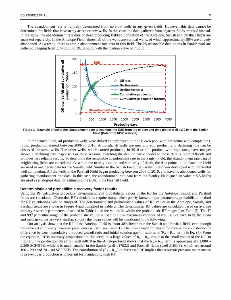
To estimate the EUR, the abandonment rate is required. The abandonment rate is the last oil rate delivered before the well is abandoned. This rate is used as a cut-off point to estimate the EUR from the oil rate and time plot (see example in Figure 3).

From To

Initial reservoir pressure (psia) P 4,060 7,325 5,700 Cramer (1986) and Wang et al. (2010)

Reservoir temperature (F) T 175 250 210 Kuhn et al. (2009)

Oil API gravity (degree API) API 39 45 2,300 Breit et al. (1992)

Gas specific gravity γg 0.77 0.88 0.83 Breit et al. (1992)

Bubble-point pressure (psia) Pb 1,730 2,900 2,300 Breit et al. (1992) and Clark (2009)

Initial water saturation (decimal) Swi 0.20 0.50 0.35 Bohrer et al. (2008)

Water salinity (ppm) Sal 2,000 471,000 237,000 Palombi et al. (2006)

Porosity (decimal) φ 0.01 0.16 0.09 Pitman et al. (2001)

ValuesParameters Symbol ReferencesAverage

CSUG/SPE 149471 5

The abandonment rate is normally determined from no flow wells in any given fields. However, this data cannot be determined for fields that have many active or new wells. In this case, the data gathered from adjacent fields are used instead. In the study, the abandonment rate data of three producing Bakken Formation of the Antelope, Sanish and Parshall fields are analyzed separately. In the Antelope Field, almost all of the wells are vertical wells, of which approximately 80% are already abandoned. As a result, there is ample abandonment rate data in this field. The 26 reasonable data points in Sanish pool are gathered, ranging from 1.74 bbl/d to 19.13 bbl/d, with the median value of 7 bbl/d.

Figure 3 - Example of using the abandonment rate to estimate the EUR from the oil rate and time plot of well #17240 in the Sanish

Field (Data from NDIC website).

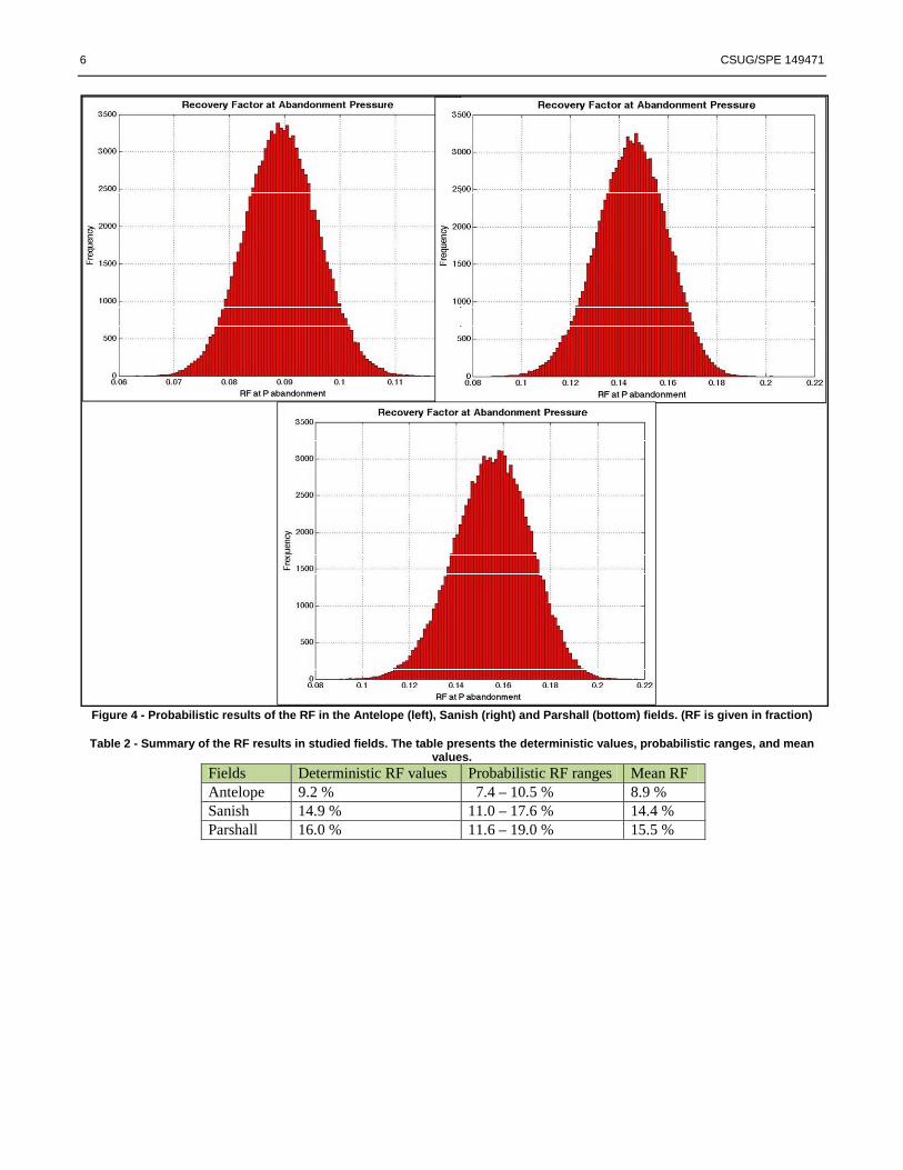
In the Sanish Field, all producing wells were drilled and produced in the Bakken pool with horizontal well completions. Initial production started between 2006 to 2010. Although, all wells are new and still producing, a declining rate can be observed for some wells. The other wells, which started producing in 2010 or still produce with high rates, have not yet shown a declining rate response. For these reasons, matching the decline curve model to these data is more difficult and provides less reliable results. To determine the reasonable abandonment rate in the Sanish Field, the abandonment rate data of neighboring fields are considered. Based on the nearby location and similarity of depth, the data points in the Antelope Field are used as analogous data for the Sanish Field. Similar to the Sanish Field, the Parshall Field was developed with horizontal well completion. All the wells in the Parshall Field began producing between 2006 to 2010, and have no abandoned wells for gathering abandonment rate data. In this case, the abandonment rate data from the Stanley Field (median value = 5.5 bbl/d) are used as analogous data for estimating the EUR in the Parshall Field. Deterministic and probabilistic recovery factor results Using the RF calculation procedure, deterministic and probabilistic values of the RF for the Antelope, Sanish and Parshall fields are calculated. Given that RF calculations require many, often poorly known, input parameters, probabilistic method for RF calculations will be analyzed. The deterministic and probabilistic values of RF values in the Antelope, Sanish, and Parshall fields are shown in Figure 4 and compiled in Table 2. The deterministic RF values are calculated based on average primary reservoir parameters presented in Table 1 and the values lie within the probabilistic RF ranges (see Table 2). The 1st and 99th percentile range of the probabilistic values is used to allow maximum variance of results. For each field, the mean and median values are very similar, so only the mean values will be mentioned in the following.

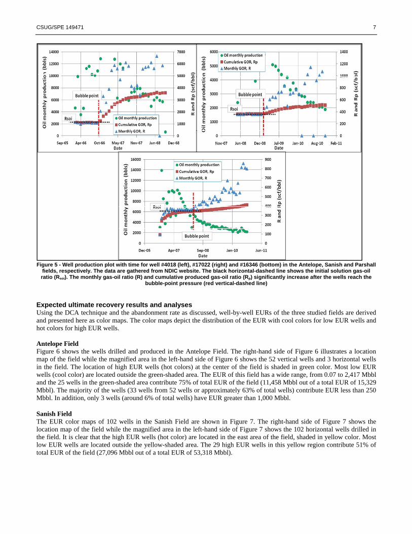
Our analysis show that the RF of the Antelope Field is about 40% lower than the Sanish and Parshall fields even though the same set of primary reservoir parameters is used (see Table 1). The main reason for this difference is the contribution of difference between cumulative produced gas-oil ratio and initial solution gas-oil ratio term (Rp – Rsoi term) in Eq. (5). From the equation, RF is inversely proportional to this term; thus large values of Rp – Rsoi result in the small values of the RF. In Figure 5, the production data from well #4018 in the Antelope Field shows that the Rp – Rsoi term is approximately 1,000 – 2,500 SCF/STB, while it is much smaller in the Sanish (well #17022) and Parshall fields (well #16346), which are around 100 – 200 and 70 -100 SCF/STB. The contribution of (Rp – Rsoi) to decreased RF implies that reservoir pressure maintenance to prevent gas production is important for maintaining high RF.

0

50

100

150

200

0 500 1000 1500 2000 2500 3000 3500 4000

Oil rate (b

bl/d) and cumulative oil 

prod

uction

 (Mbb

l)

Producing days

Oil rateDecline matchDecline forecastCumulative productionCumulative production forecast

Abandonment rate

EUR

6 CSUG/SPE 149471

Figure 4 - Probabilistic results of the RF in the Antelope (left), Sanish (right) and Parshall (bottom) fields. (RF is given in fraction)

Table 2 - Summary of the RF results in studied fields. The table presents the deterministic values, probabilistic ranges, and mean values.

Fields Deterministic RF values Probabilistic RF ranges Mean RF Antelope 9.2 % 7.4 – 10.5 % 8.9 % Sanish 14.9 % 11.0 – 17.6 % 14.4 % Parshall 16.0 % 11.6 – 19.0 % 15.5 %

CSUG/SPE 149471 7

Figure 5 - Well production plot with time for well #4018 (left), #17022 (right) and #16346 (bottom) in the Antelope, Sanish and Parshall

fields, respectively. The data are gathered from NDIC website. The black horizontal-dashed line shows the initial solution gas-oil ratio (Rsoi). The monthly gas-oil ratio (R) and cumulative produced gas-oil ratio (Rp) significantly increase after the wells reach the

bubble-point pressure (red vertical-dashed line)

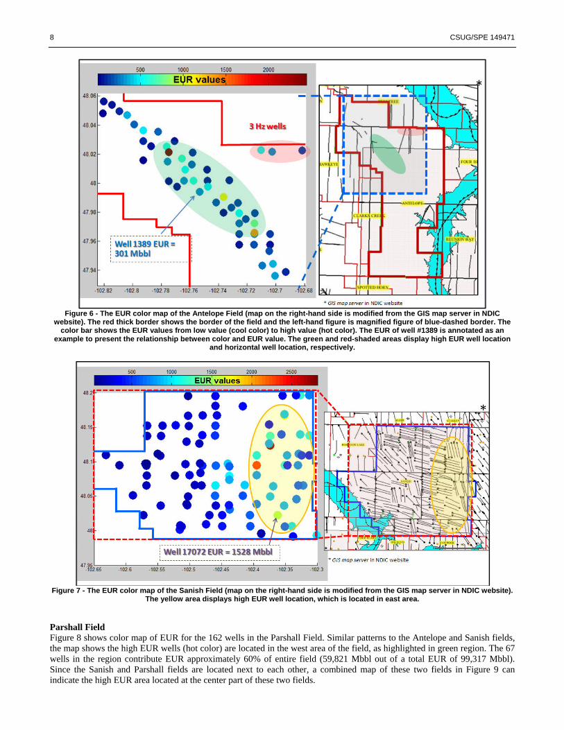
Expected ultimate recovery results and analyses Using the DCA technique and the abandonment rate as discussed, well-by-well EURs of the three studied fields are derived and presented here as color maps. The color maps depict the distribution of the EUR with cool colors for low EUR wells and hot colors for high EUR wells. Antelope Field Figure 6 shows the wells drilled and produced in the Antelope Field. The right-hand side of Figure 6 illustrates a location map of the field while the magnified area in the left-hand side of Figure 6 shows the 52 vertical wells and 3 horizontal wells in the field. The location of high EUR wells (hot colors) at the center of the field is shaded in green color. Most low EUR wells (cool color) are located outside the green-shaded area. The EUR of this field has a wide range, from 0.07 to 2,417 Mbbl and the 25 wells in the green-shaded area contribute 75% of total EUR of the field (11,458 Mbbl out of a total EUR of 15,329 Mbbl). The majority of the wells (33 wells from 52 wells or approximately 63% of total wells) contribute EUR less than 250 Mbbl. In addition, only 3 wells (around 6% of total wells) have EUR greater than 1,000 Mbbl.

Sanish Field The EUR color maps of 102 wells in the Sanish Field are shown in Figure 7. The right-hand side of Figure 7 shows the location map of the field while the magnified area in the left-hand side of Figure 7 shows the 102 horizontal wells drilled in the field. It is clear that the high EUR wells (hot color) are located in the east area of the field, shaded in yellow color. Most low EUR wells are located outside the yellow-shaded area. The 29 high EUR wells in this yellow region contribute 51% of total EUR of the field (27,096 Mbbl out of a total EUR of 53,318 Mbbl).

8 CSUG/SPE 149471

Figure 6 - The EUR color map of the Antelope Field (map on the right-hand side is modified from the GIS map server in NDIC

website). The red thick border shows the border of the field and the left-hand figure is magnified figure of blue-dashed border. The color bar shows the EUR values from low value (cool color) to high value (hot color). The EUR of well #1389 is annotated as an

example to present the relationship between color and EUR value. The green and red-shaded areas display high EUR well location and horizontal well location, respectively.

Figure 7 - The EUR color map of the Sanish Field (map on the right-hand side is modified from the GIS map server in NDIC website).

The yellow area displays high EUR well location, which is located in east area.

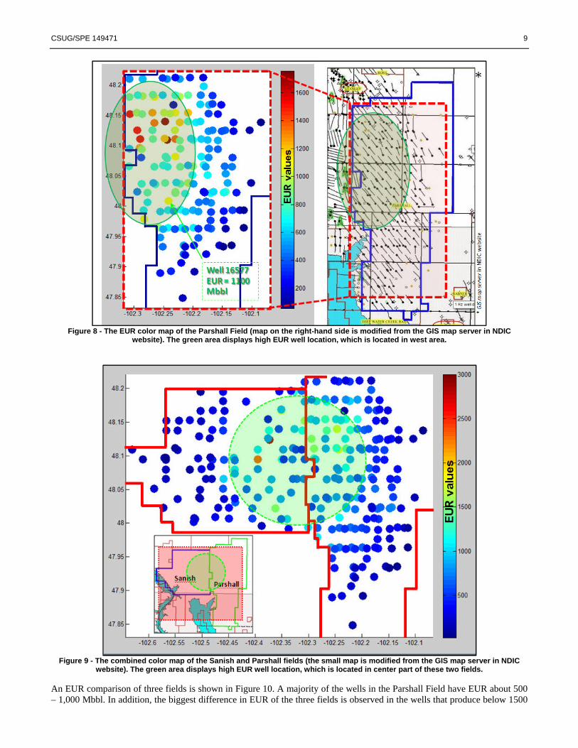
Parshall Field Figure 8 shows color map of EUR for the 162 wells in the Parshall Field. Similar patterns to the Antelope and Sanish fields, the map shows the high EUR wells (hot color) are located in the west area of the field, as highlighted in green region. The 67 wells in the region contribute EUR approximately 60% of entire field (59,821 Mbbl out of a total EUR of 99,317 Mbbl). Since the Sanish and Parshall fields are located next to each other, a combined map of these two fields in Figure 9 can indicate the high EUR area located at the center part of these two fields.

CSUG/SPE 149471 9

Figure 8 - The EUR color map of the Parshall Field (map on the right-hand side is modified from the GIS map server in NDIC

website). The green area displays high EUR well location, which is located in west area.

Figure 9 - The combined color map of the Sanish and Parshall fields (the small map is modified from the GIS map server in NDIC

website). The green area displays high EUR well location, which is located in center part of these two fields.

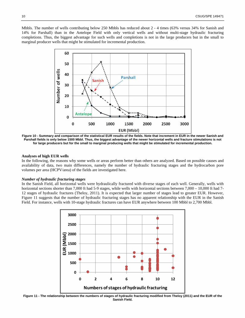
An EUR comparison of three fields is shown in Figure 10. A majority of the wells in the Parshall Field have EUR about 500 – 1,000 Mbbl. In addition, the biggest difference in EUR of the three fields is observed in the wells that produce below 1500

10 CSUG/SPE 149471

Mbbls. The number of wells contributing below 250 Mbbls has reduced about 2 - 4 times (63% versus 34% for Sanish and 14% for Parshall) than in the Antelope Field with only vertical wells and without multi-stage hydraulic fracturing completions. Thus, the biggest advantage for such wells and completions is not in the large producers but in the small to marginal producer wells that might be stimulated for incremental production.

Figure 10 - Summary and comparison of the statistical EUR results of the fields. Note that increment in EUR in the newer Sanish and

Parshall fields is only below 1500 Mbbl. Thus, the biggest advantage of the newer horizontal wells and fracture stimulations is not for large producers but for the small to marginal producing wells that might be stimulated for incremental production.

Analyses of high EUR wells In the following, the reasons why some wells or areas perform better than others are analyzed. Based on possible causes and availability of data, two main differences, namely the number of hydraulic fracturing stages and the hydrocarbon pore volumes per area (HCPV/area) of the fields are investigated here. Number of hydraulic fracturing stages In the Sanish Field, all horizontal wells were hydraulically fractured with diverse stages of each well. Generally, wells with horizontal sections shorter than 7,000 ft had 5-9 stages, while wells with horizontal sections between 7,000 – 10,000 ft had 7-12 stages of hydraulic fractures (Theloy, 2011). It is expected that larger number of stages lead to greater EUR. However, Figure 11 suggests that the number of hydraulic fracturing stages has no apparent relationship with the EUR in the Sanish Field. For instance, wells with 10-stage hydraulic fractures can have EUR anywhere between 100 Mbbl to 2,700 Mbbl.

Figure 11 - The relationship between the numbers of stages of hydraulic fracturing modified from Theloy (2011) and the EUR of the

Sanish Field.

0

500

1000

1500

2000

2500

3000

0 2 4 6 8 10 12

EUR (M

bbl)

Numbers of stages of hydraulic fracturing

CSUG/SPE 149471 11

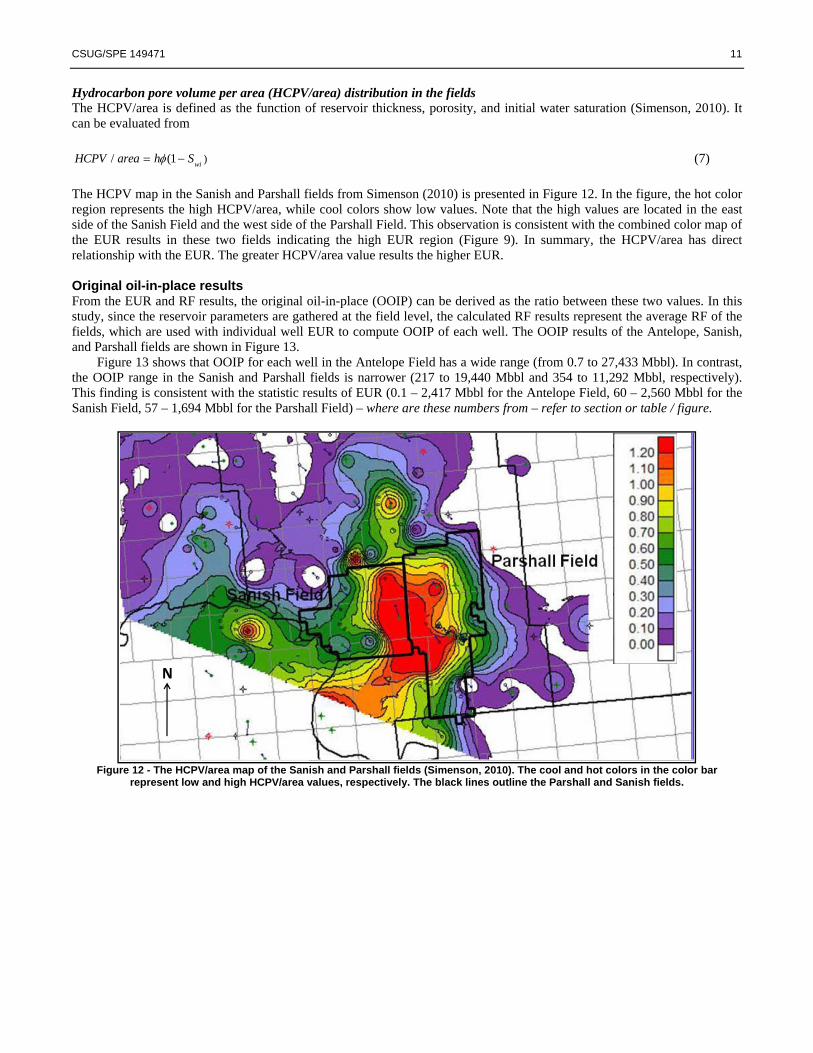
Hydrocarbon pore volume per area (HCPV/area) distribution in the fields The HCPV/area is defined as the function of reservoir thickness, porosity, and initial water saturation (Simenson, 2010). It can be evaluated from

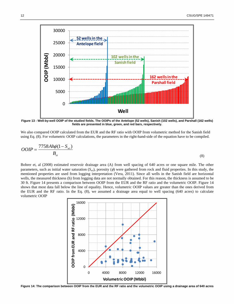
)/ (1 wiHCPV area h Sφ= − (7) The HCPV map in the Sanish and Parshall fields from Simenson (2010) is presented in Figure 12. In the figure, the hot color region represents the high HCPV/area, while cool colors show low values. Note that the high values are located in the east side of the Sanish Field and the west side of the Parshall Field. This observation is consistent with the combined color map of the EUR results in these two fields indicating the high EUR region (Figure 9). In summary, the HCPV/area has direct relationship with the EUR. The greater HCPV/area value results the higher EUR. Original oil-in-place results From the EUR and RF results, the original oil-in-place (OOIP) can be derived as the ratio between these two values. In this study, since the reservoir parameters are gathered at the field level, the calculated RF results represent the average RF of the fields, which are used with individual well EUR to compute OOIP of each well. The OOIP results of the Antelope, Sanish, and Parshall fields are shown in Figure 13.

Figure 13 shows that OOIP for each well in the Antelope Field has a wide range (from 0.7 to 27,433 Mbbl). In contrast, the OOIP range in the Sanish and Parshall fields is narrower (217 to 19,440 Mbbl and 354 to 11,292 Mbbl, respectively). This finding is consistent with the statistic results of EUR (0.1 – 2,417 Mbbl for the Antelope Field, 60 – 2,560 Mbbl for the Sanish Field, 57 – 1,694 Mbbl for the Parshall Field) – where are these numbers from – refer to section or table / figure.

Figure 12 - The HCPV/area map of the Sanish and Parshall fields (Simenson, 2010). The cool and hot colors in the color bar

represent low and high HCPV/area values, respectively. The black lines outline the Parshall and Sanish fields.

N

12 CSUG/SPE 149471

Figure 13 - Well-by-well OOIP of the studied fields. The OOIPs of the Antelope (52 wells), Sanish (102 wells), and Parshall (162 wells)

fields are presented in blue, green, and red bars, respectively.

We also compared OOIP calculated from the EUR and the RF ratio with OOIP from volumetric method for the Sanish field using Eq. (8). For volumetric OOIP calculations, the parameters in the right-hand-side of the equation have to be compiled.

7758 (1 )wi

oi

Ah SOOIPBφ −

= (8)

Bohrer et, al (2008) estimated reservoir drainage area (A) from well spacing of 640 acres or one square mile. The other parameters, such as initial water saturation (Swi), porosity (φ) were gathered from rock and fluid properties. In this study, the mentioned properties are used from logging interpretation (Vera, 2011). Since all wells in the Sanish field are horizontal wells, the measured thickness (h) from logging data are not normally obtained. For this reason, the thickness is assumed to be 30 ft. Figure 14 presents a comparison between OOIP from the EUR and the RF ratio and the volumetric OOIP. Figure 14 shows that most data fall below the line of equality. Hence, volumetric OOIP values are greater than the ones derived from the EUR and the RF ratio. In the Eq. (8), we assumed a drainage area equal to well spacing (640 acres) to calculate volumetric OOIP

Figure 14: The comparison between OOIP from the EUR and the RF ratio and the volumetric OOIP using a drainage area of 640 acres

0

5000

10000

15000

20000

25000

30000

OOIP (M

bbl)

Well 

52 wells in the Antelope field

102 wells in the Sanish field

162 wells in the Parshall field

0

4000

8000

12000

16000

0 4000 8000 12000 16000

OOIP from

 EUR and

 RF ratio  (M

bbl)

Volumetric OOIP (Mbbl)

CSUG/SPE 149471 13

Figure 14 suggests the assumed drainage area should be reduced to make the OOIP from these two approaches match each other. Thus, the proper drainage area should be much less than 640 acres. One direct implication is to optimize the typical well spacing of 640 acres and investigate efficiency of an infill drilling program. Conclusions We have analyzed RF, EUR, and OOIP of the Bakken Formation. We have also investigated the effects of various input data required to make the calculations of RF. Our results and analyses show that:

• From deterministic and probabilistic analyses, the RF of Parshall Field (16%) is higher than that of the Antelope (9.2%) and Sanish (14.9%) fields.

• Well production data shows that this term is lowest in the Parshall Field because its cumulative produced gas-oil ratio (Rp) is low. As a result, the RF of the Parshall Field is the highest among the studied fields.

• The contribution of (Rp – Rsoi) to decreased RF implies that reservoir pressure maintenance to prevent gas production is important for maintaining high RF.

• In the Antelope Field, the high EUR area is located in the center of the field. High EUR areas in the Sanish and Parshall fields are located in the east (Sanish) and west side (Parshall).

• The number of hydraulic fracturing stages has no apparent relationship with EUR. However, hydrocarbon pore volume per area (HCPV/area) shows a direct relation to EUR.

• The Antelope Field shows a larger range of OOIP per well from the EUR and the RF ratio. In contrast, the distribution of OOIP per well in the Parshall Field is much smaller.

• A comparison between OOIP derived from two different methods shows the assumed drainage area might be much less than the current well spacing of 640 acres. An optimization of the well spacing and investigation of an infill drilling program should be considered.

Acknowledgements Authors would like to express gratitude to Craig Van Kirk and Stephen Sonnenberg (Colorado School of Mines), Chet Ozgen (NITEC LLC Company), Andrea Simenson (Discovery Group Company), Cosima Theloy, Ryan Vera, Baoqing Xu, and John Akinboyewa (Colorado School of Mines) for their input, guidance discussions, and comments. We also thank Chevron Thailand Business Unit for sponsorship and financial support of Mr. Dechongkit for his entire education program. Nomenclature A = Reservoir Drainage Area, acre API = API Oil Gravity, degree API Bg = Gas Formation Volume Factor, bbl/SCF Bgi = Initial Gas Formation Volume Factor, bbl/SCF Bo = Oil Formation Volume Factor, bbl/STB Bob = Oil Formation Volume Factor at Bubble-Point Pressure, bbl/STB Boi = Initial Oil Formation Volume Factor, bbl/STB Bt = Total Formation Volume Factor, bbl/STB Bti = Initial Total Formation Volume Factor, bbl/STB Bw = Water Formation Volume Factor, bbl/STB b = Arps Decline Curve Exponent, dimensionless co = Oil Isothermal Compressibility, psi-1 cw = Water Isothermal Compressibility, psi-1 cf = Formation Isothermal Compressibility, psi-1 Di = Rate of Decline, day-1

EUR = Expected Ultimate Recovery of Oil, Mbbl HCPV/area = Hydrocarbon Pore Volume Per Area, ft h = Reservoir Thickness, ft m = Ratio of Initial Gas Cap Volume to Initial Oil Volume,dimensionless N = Original Oil-In-Place, STB

Np = Cumulative Oil Production, STB OOIP = Original Oil-In-Place, Mbbl P = Reservoir Pressure, psia Pb = Bubble-Point Pressure, psia Pi = Initial Reservoir Pressure, psia ΔP = Reservoir Pressure drop, psia q = Producing Oil Rate, bbl/d qi = Initial Producing Oil Rate of DCA Model, bbl/d R = Monthly Produced Gas-Oil Ratio, SCF/STB

14 CSUG/SPE 149471

Rso = Solution Gas-Oil Ratio, SCF/STB Rsob = Solution Gas-Oil Ratio at Bubble-Point Pressure, SCF/STB Rsoi = Initial Solution Gas-Oil Ratio, SCF/STB Rp = Cumulative Produced Gas-Oil Ratio, SCF/STB Swi = Initial Water Saturation, decimal Sal = Water Salinity, ppm T = Reservoir Temperature, degree F t = Time, day(s) We = Water Encroachment, bbl

Wp = Cumulative Water Production, STB Greek symbols φ = Porosity, decimal γg = Gas Specific Gravity, dimensionless References Ahmed, T. 2007. Equation of State and PVT Analysis , Applications for Improved Reservoir Modeling. Gulf Publishing Company,

Houston, Texas. Bohrer, M., Fried, S., Helms, L., Hicks, B., Juenker, B., McCusker, D., Anderson F., LeFever, J., Murphy, E., and Nordeng S. 2008. State

of North Dakota Bakken Formation Resources Study Project. Appendix C, April. Breit, V.S., Stright Jr, D.H., and Dozzo, J.A. 1992. Reservoir Characterization of the Bakken Shale from Modeling of Horizontal Well

Production Interference Data. SPE 24320 presented at the SPE Rocky Mountain Regional Meeting, Casper, Wyoming, May 18-21. Brown, M., Ozkan, E., Raghavan, R., and Kazemi, H. 2009. Practical Solutions for Pressure Transient Responses of Fractured Horizontal

Wells in Unconventional Reservoirs. SPE 125043 presented at the 2009 SPE Annual Technical Conference and Exhibition, New Orleans, Louisiana. October 4-7.

Cheng, Y., Lee, W.J., and McVay, D.A. 2008. Quantification of Uncertainty in Reserve Estimation from Decline Curve Analysis of Production Data for Unconventional Reservoirs. Journal of Energy Resources Technology, December. Vol. 130.

Chilingar, G.V., Rieke, H.H. III, and Sawabini, C.T. 1970. Compressibilities of the Clays and Some Means of Predicting and Preventing Subsidence. Publication International Association Scientist Hydrology Symposium, Tokyo. No.89, pp. 377-393.

Clark, Aaron J. 2009. Determination Recovery Factor in the Bakken Formation, Mountrail Country, ND. SPE 133719 presented at the 2009 SPE International Student Paper Contest at the SPE Annual Technical Conference and Exhibition, New Orleans, Louisiana, October 4-7.

Craft, B.C., and Hawkins, M. Revised by Terry, E. 1991. Applied Petroleum Reservoir Engineering. Second Edition. Upper Saddle River, New Jersey: Prentice Hall.

Cramer, D.D. 1986. Reservoir Characteristics and Stimulation Techniques in the Bakken Formation and Adjacent Beds, Billings Nose Area, Williston Basin. SPE 15166 presented at the SPE Rocky Mountain Regional Meeting, Billings, MT, May 19-21. Dake, L.P. 2001. The Practical of Reservoir Engineering (Revised Edition). Elsevier publications. Oxford, UK.

Finch, W.C.1969. Abnormal Pressure in the Antelope Field, North Dakota. Journal of Petroleum Technology, July. pp. 821-826. Folsom, C.B. Jr., Carlson, C.G., and Anderson, S.B. 1959. Preliminary Report on the Antelope-Madison and Antelope-Sanish Pools. North Dakota Geological Survey, Report of Investigation Number 32.

Fox, J.N., and Martiniuk, C.D. 1994. Reservoir Characteristics and Petroleum Potential of the Bakken Formation, Southwestern Manitoba. JCPT journal, October. Vol 33, No. 8.

Hassler, G., Poohkay, P., and Jubinville, L. 2009. A Comparative Analysis of Multi-Stage Fracture Stimulation Treatments within the Bakken Formation, Kisbey Area, SE Sask. TriStar Oil&Gas Ltd, April.

Houston, M., McCallister, M., Jany, J., and Audet, J. 2010. Next Generation Multi-Stage Completion Technology and Risk Sharing Accelerates Development of the Bakken Play. SPE 135584 presented at the SPE Annual Technical Conference and Exhibition, Florence, Italy. September 19-22.

Johnson, S. 1990. Bakken Shale. Oil and Gas Investor, Hart Publications Inc, June, pp.36. Kuhn, P.P., Di Primio, R., and Horsfield, B. 2009. Petroleum System of the Bakken Formation Do the Hydrocarbon Migrate?. PhD Day 2009, Organic Geochemistry Section 4.3, Technical University of Berin – 26th Month.

Kuhn, P.P., Di Primio, R., and Horsfield, B.. 2009. Petroleum System of the Bakken Formation Do the Hydrocarbon Migrate?. PhD Day 2009, Organic Geochemistry Section 4.3, Technical University of Berin – 26th Month.

LeFever J., and Helms L. 2006. Bakken Formation Reserve Estimates. North Dakota Geological Survey Publication, Petroleum information. July.

Meissner, F.F. 1978. Petroleum Geology of the Bakken Formation Williston Basin, North Dakota and Montana. The Williston Basin Symposium, The Montana Geological Society, 24th Annual Conference, Billings, Montana.

Minhas, H., Matteo, E., Eikeland, K.M., Mengoli, M., and Beswetherick, S. 2005. Probabilistic Reserve Estimation Constrained by Limited Production Data: An Integrated Approach. IPTC 10957 presented at the International Petroleum Technology Conference, Doha, Qatar, November 21-23.

Murray G.H., Jr. 1968. Quantitative Fracture Study-Sanish Pool, McKenzie County, North Dakota. The American Association of Petroleum Geologists Bulletin, Vol 52, No.1, January. pp. 57-65.

Official Portal for North Dakota State Government, North Dakota Geological Survey. https://www.dmr.nd.gov/oilgas/. Ozkan, E., Raghavan, R., and Apaydin, O.G. 2010. Modeling of Fluid Transfer from Shale Matrix to Fracture Network. SPE 134830

presented at the SPE Annual Technical Conference and Exhibition, Florence, Italy. September 19-22.

CSUG/SPE 149471 15

Palombi, D.D., and Rostron, B.J. 2006. Deep Regional Fluid Flow in the North Eastern Flank of the Williston Basin: Implications for Hydrocarbon Migration. The 2006 AAPG International Conference and Exhibition, Perth, Australia. November 8.

Pitman, J.K., Price, L.C., and LeFever, J.A. 2001. Diagenesis and Fracture Development in the Bakken Formation, Williston Basin: Implications for the Reservoir Quality in the Middle Member. USGS Professional Paper 1653, November.

Pollastro, R.M., Cook, T.A., Roberts, L.N.R., Schenk, C.J., Lewan, M.D., Anna, L.O., Gaswirth, S.B., Lillis, P.G., Klett, T.R., and Charpentier, R.R. 2008. Assessment of undiscovered oil resources in the Devonian-Mississippian Bakken Formation, Williston Basin Province, Montana and North Dakota. U.S. Geological Survey Fact Sheet, pp.2.

Poston, S.W., and Poe, B.D., Jr. 2008. Analysis of Production Decline Curve. Society of Petroleum Engineering. Texas.Reisz, M.R. 1992. Reservoir Evaluation of Horizontal Bakken Well Performance on the Southwestern Flank of the Williston Basin. SPE 22389 presented at SPE International Meeting on Petroleum Engineering, Beijing, China, March 24-27.

Simenson, A. 2010. Depositional Facies and Petrophysical Analysis of the Bakken Formation, Parshall Field, Mountrail County, North Dakota. MS thesis. Department of Geology, Colorado School of Mines, Golden, Colorado.

Theloy, C. 2011. Contribution of Natural Fractures to Production Sanish Field, North Dakota. Bakken Consortium Meeting, Golden, Colorado. April 20.

Wang, X., Luo, P., Er, V., and Huang, S. 2010. Assessment of CO2 Flooding Potential for Bakken Formation, Saskatchewan. CSUG/SPE 137728 presented at the Canadian Unconventional Resources & International Petroleum Conference, Calgary, Alberta, October 19-21.

Zargari, S., and Mohaghegh, S.D. 2010. Field Development Strategies for Bakken Shale Formation. SPE 139032 presented at SPE Eastern Regional Meeting, West Virginia, October 12-14.