CSC263 Week 8Larry Zhang

http://goo.gl/forms/S9yie3597B

Announcements (strike related)

➔ Lectures go as normal

➔ Tutorial this week◆ everyone go to BA3012 (T8, F12, F2, F3)

➔ Problem sets / Assignments are submitted as normal.◆ marking may be slower

➔ Midterm: still being marked

➔ Keep a close eye on announcements

This week’s outline

➔ Graph

➔ BFS

A really, really important ADT that is used to model relationships between objects.

Graph

Reference: http://steve-yegge.blogspot.ca/2008/03/get-that-job-at-google.html

Things that can be modelled using graphs

➔ Web➔ Facebook➔ Task scheduling➔ Maps & GPS➔ Compiler (garbage collection)➔ OCR (computer vision)➔ Database➔ Rubik’s cube➔ …. (many many other things)

Definition

G = (V, E)Set of vertices

e.g., {a, b, c}Set of edges

e.g., { (a, b), (c, a) }

Flavours of graphs

Undirected Directed

each edge is an unordered pair (u, v) = (v, u)

each edge is an ordered pair (u, v) ≠ (v, u)

10 200

-3

Unweighted Weighted

Simple Non-simple

No multiple edge, no self-loop

Acyclic Cyclic

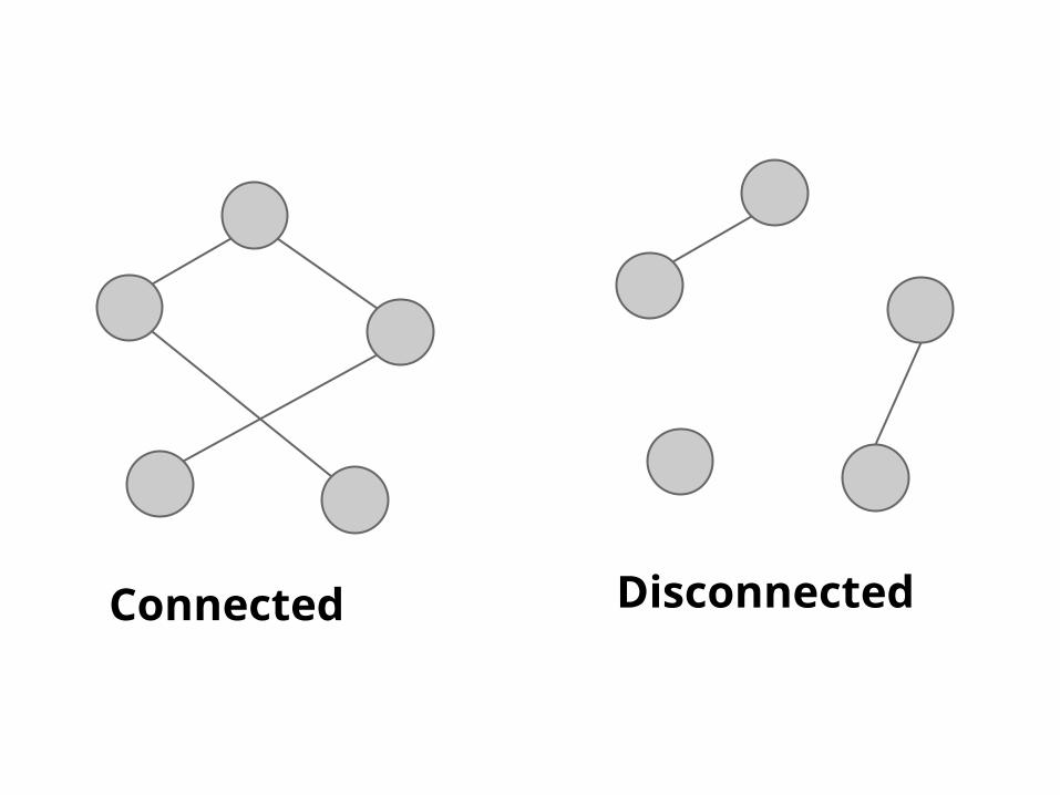
Connected Disconnected

Dense Sparse

Path

Length of path = number of edges

A path of length 3

Read Appendix B.4 for more background on graphs.

Operations on a graph

➔ Add a vertex; remove a vertex

➔ Add an edge; remove an edge

➔ Get neighbours (undirected graph)◆ Neighbourhood(u): all v ∈ V such that (u, v) ∈ E

➔ Get in-neighbours / out-neighbours (directed graph)

➔ Traversal: visit every vertex in the graph

Data structures for the graph ADT

➔ Adjacency matrix➔ Adjacency list

Adjacency matrix

A |V|x|V| matrix A

Adjacency matrix

1

3

42

1 2 3 4

1

2

3

4

1 1

1

1

0 0

0 0 0

0 0 0

0 0 0 0

1 2 3 4

1

2

3

4

1 1

1

1

0 0

0 0 0

0 0 0

0 0 0 0

How much space does it take?

|V|²

Adjacency matrix

Adjacency matrix (undirected graph)

1

3

42

1 2 3 4

1

2

3

4

1 1

1

1

0 1

1 0 0

1 0 0

1 0 0 0

The adjacency matrix of an undirected graph is _________________.symmetric

1 2 3 4

1

2

3

4

1 1

1

1

0 1

1 0 0

1 0 0

1 0 0 0

Adjacency matrix (undirected graph)

How much space does it take?

|V|²

Adjacency list

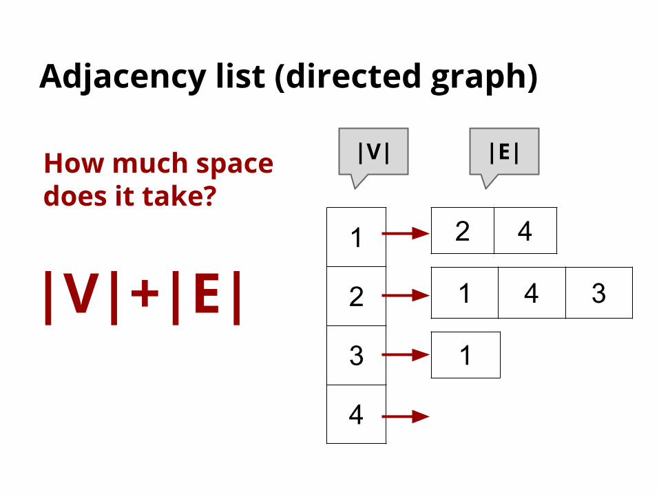
Adjacency list (directed graph)

Each vertex vi stores a list A[i] of vj that satisfies (vi, vj) ∈ E

1

2

3

4

2 4

1

1

3

42

1 4 3

1

2

3

4

2 4

1

1 4 3

Adjacency list (directed graph)

How much space does it take?

|V|+|E|

|V| |E|

Adjacency list (undirected graph)

1

3

42

1

2

3

4

2 4 3

1 3

2 1

1

1

2

3

4

2 4 3

1 3

2 1

1

Adjacency list (undirected graph)

How much space does it take?

|V|+2|E|

|V| 2|E|

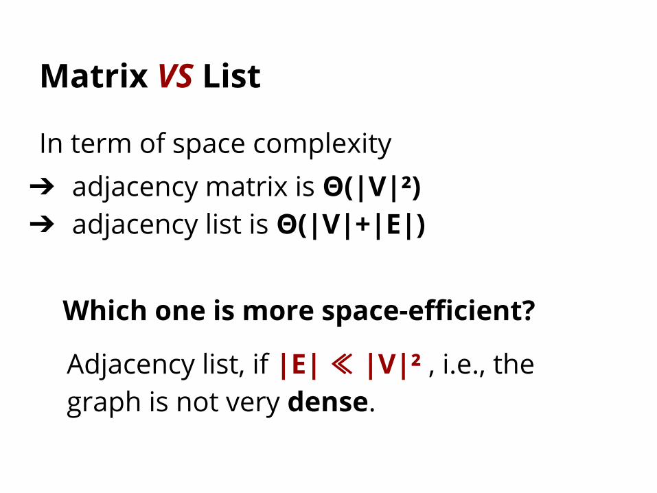
Matrix VS List

In term of space complexity➔ adjacency matrix is Θ(|V|²)➔ adjacency list is Θ(|V|+|E|)

Which one is more space-efficient?

Adjacency list, if |E| ≪ |V|² , i.e., the graph is not very dense.

Matrix VS List

Anything that Matrix does better than List?

Check whether edge (vi, vj) is in E➔ Matrix: just check if A[i, j] = 1, O(1)➔ List: go through list A[i] see if j is in

there, O(length of list)

Takeaway

Adjacency matrix or adjacency list?

Choose the more appropriate one depending on the problem.

CSC263 Week 8Wednesday / Thursday

Announcements

➔ PS6 posted, due next Tuesday as usual

➔ Drop date: March 8th

Recap

➔ ADT: Graph

➔ Data structures

◆ Adjacency matrix

◆ Adjacency list

➔ Graph operations

◆ Add vertex, remove vertex, …, edge query, …

◆ Traversal

Graph Traversals

They are twins!

BFS and DFS

Graph traversals

Visiting every vertex once, starting from a given vertex.

The visits can follow different orders, we will learn about the following two ways➔ Breadth First Search (BFS)➔ Depth First Search (DFS)

Intuitions of BFS and DFS

Consider a special graph -- a tree

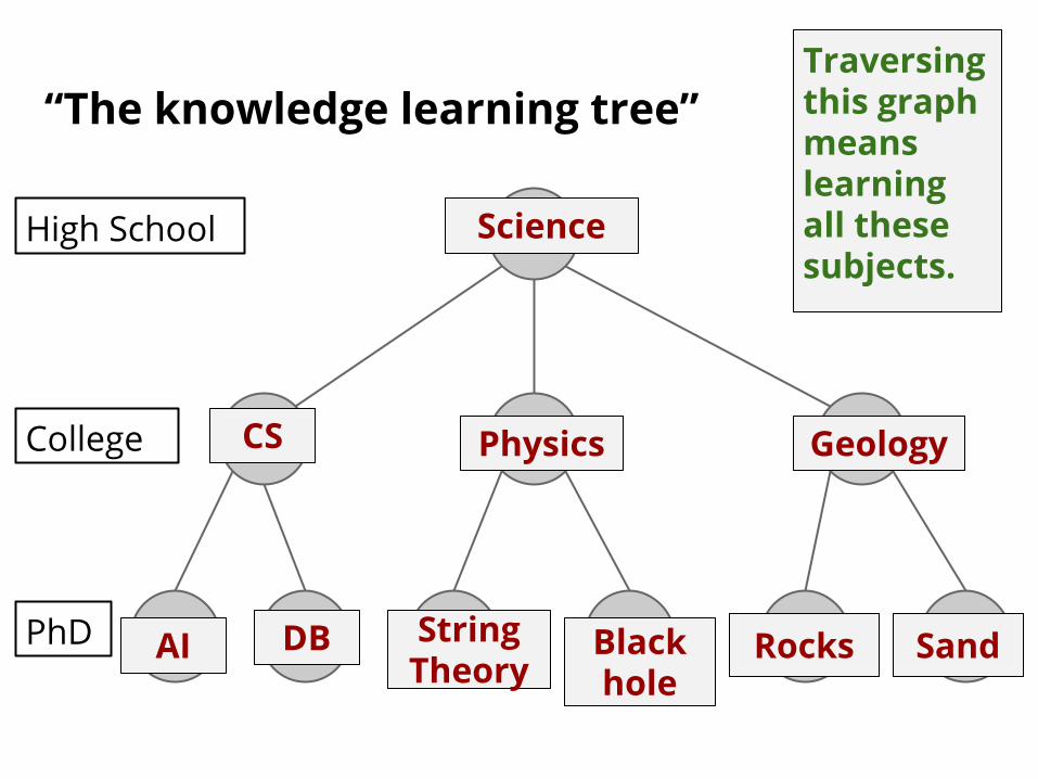
“The knowledge learning tree”

High School

College

PhD

Science

CS Physics Geology

AI DB String Theory

Black hole

Rocks Sand

Traversing this graph means learning all these subjects.

The Breadth-First ways of learning these subjects ➔ Level by level, finish high school, then all subjects at

College level, then finish all subjects in PhD level.

High School

College

PhD

Science

CS Physics Geology

AI DB String Theory

Black hole

Rocks Sand

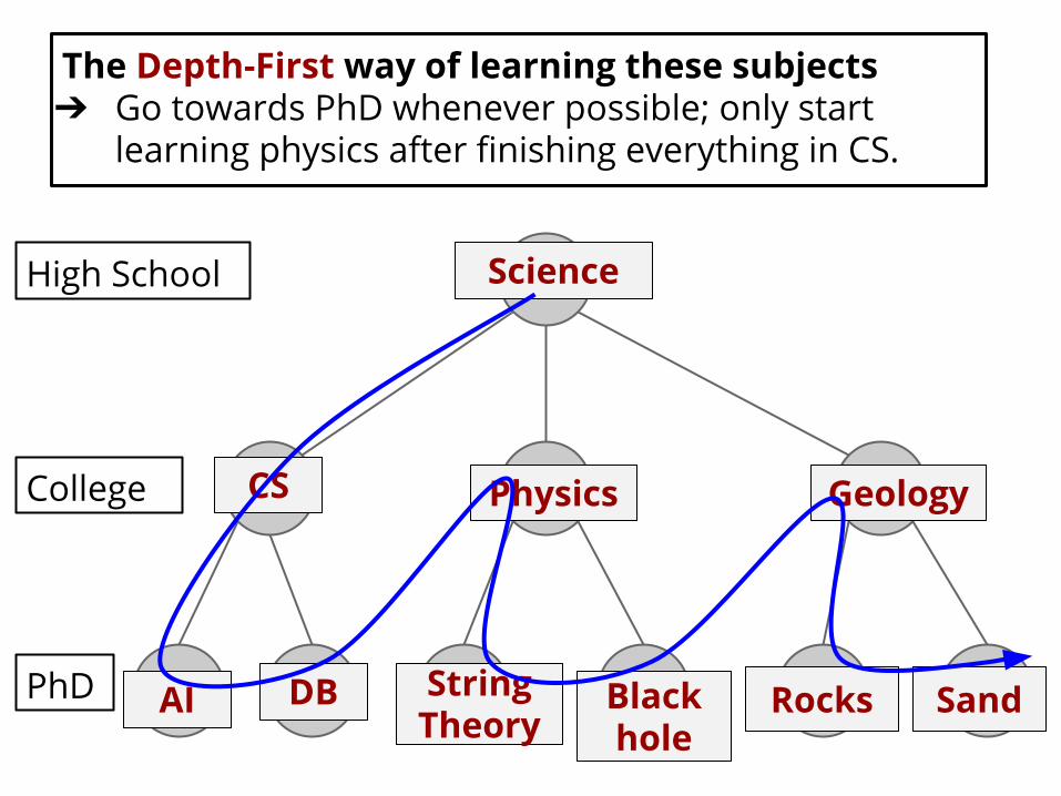
The Depth-First way of learning these subjects ➔ Go towards PhD whenever possible; only start

learning physics after finishing everything in CS.

High School

College

PhD

Science

CS Physics Geology

AI DB String Theory

Black hole

Rocks Sand

Now let’s seriously start studying BFS

Review CSC148:BFS in a tree (starting from root) is a ______________________ traversal.

Special case: BFS in a tree

level-by-level

What ADT did we use for implementing the level-by-level traversal?

Queue!

(NOT preorder!)

Special case: BFS in a tree

NOT_YET_BFS(root):

Q ← Queue()

Enqueue(Q, root)

while Q not empty:

x ← Dequeue(Q)

print x

for each child c of x:

Enqueue(Q, c)

a

b c

d e f

a

DQ

bQueue: c d e f

DQ DQ DQ DQ DQEMPTY!

Output: abcdef

The real deal: BFS in a Graph

r ts

w xv

u

y

NOT_YET_BFS(root): Q ← Queue() Enqueue(Q, root) while Q not empty: x ← Dequeue(Q) print x for each neighbr c of x: Enqueue(Q, c)

If we just run NOT_YET_BFS(t) on the above graph. What problem would we have?

It would want to visit some vertex twice (e.g., x), which shall be avoided!

How avoid visiting a vertex twice

Remember you visited it by labelling it using colours.➔ White: “unvisited”➔ Gray: “encountered”➔ Black: “explored”

➔ Initially all vertices are white➔ Colour a vertex gray the first time visiting it➔ Colour a vertex black when all its neighbours

have been encountered➔ Avoid visiting gray or black vertices➔ In the end, all vertices are black (sort-of)

Some other values we want to remember during the traversal...

➔ pi[v]: the vertex from which v is encountered◆ “I was introduced as whose neighbour?”

➔ d[v]: the distance value◆ the distance from v to the source vertex of the BFS

r ts

w xv

u

y

This d[v] is going to be really useful!

Pseudocode: the real BFS

BFS(G=(V, E), s):

1 for all v in V:

2 colour[v] ← white

3 d[v] ← ∞ 4 pi[v] ← NIL

5 Q ← Queue()

6 colour[s] ← gray

7 d[s] ← 0

8 Enqueue(Q, s)

9 while Q not empty:

10 u ← Dequeue(Q)

11 for each neighbour v of u:

12 if colour[v] = white

13 colour[v] ← gray

14 d[v] ← d[u] + 1

15 pi[v] ← u

16 Enqueue(Q, v)

17 colour[u] ← black

The blue lines are the same as NOT_YET_BFS

# Initialize vertices

# start BFS by encountering the source vertex# distance from s to s is 0

# only visit unvisited vertices

# v is “1-level” farther from s than u# v is introduced as u’s neighbour

# all neighbours of u have been encountered, therefore u is explored

Let’s run an example!

r ts

w xv

u

y

BFS(G, s)

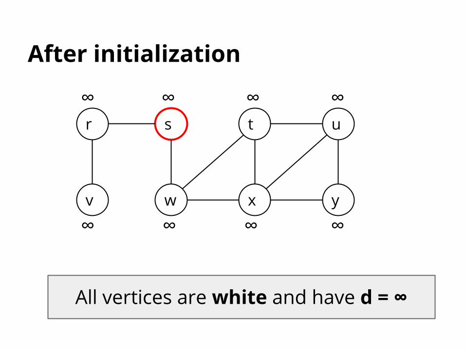
After initialization

r ts

w xv

u

y

∞∞

∞ ∞ ∞∞

∞ ∞

All vertices are white and have d = ∞

Start by “encountering” the source

r ts

w xv

u

y

∞∞

∞ ∞ ∞d=0

∞ ∞

Colour the source gray and set its d = 0, and Enqueue it

Queue: s

Dequeue, explore neighbours

r ts

w xv

u

y

∞∞

∞ ∞ ∞0

∞ ∞

Queue: s

DQ

r

1

w1

r w

The red edge indicates the pi[v] that got remembered

Colour black after exploring all neighbours

r ts

w xv

u

y

∞∞

∞ ∞ ∞0

∞ ∞

Queue: s

DQ

r

1

w1

r w

Dequeue, explore neighbours (2)

r ts

w xv

u

y

∞∞

∞ ∞ ∞0

∞ ∞

Queue: s

DQ

r

1

w1

r w

DQ

v

2

r

v

Dequeue, explore neighbours (3)

r ts

w xv

u

y

∞∞

∞ ∞ ∞0

∞ ∞

Queue: s

DQ

r

1

w1

r w

DQ

v

2

r

v

DQ

t

2

x

2

t x

w

after a few more steps...

r ts

w xv

u

y

∞∞

∞ ∞ 30

∞

Queue: s

DQ

r

1

w1

r w

DQ

2

r

v

DQ

2

2

t x

w

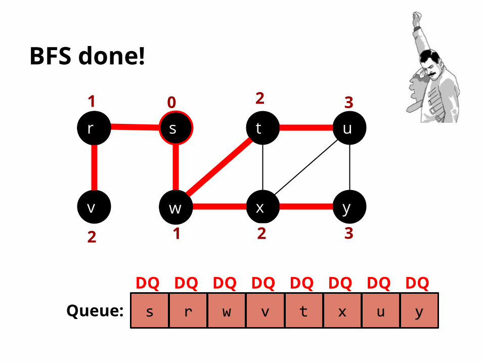
BFS done!

3

u y

DQ DQ DQ DQ DQ

What do we get after doing all these?

r ts

w xv

u

y

∞∞

∞ ∞ 30

∞

r

1

w12

r

2

2w

3

First of all, we get to visit every vertex once.

r ts

w xv

u

y

r

w

r

w

This is called the BFS-tree, it’s a tree that connects all vertices, if the graph is connected.

Did you know? The official name of the red edges are called “tree edges”.

r ts

w xv

u

y

∞∞

∞ ∞ 30

∞

r

1

w12

r

2

2w

3

These d[v] values, we said they were going to be really useful.

The value indicates the vertex’s distance from the source vertex.

Actually more than that, it’s the shortest-path distance, we can prove it.

How about finding short path itself? Follow the red edges, pi[v] comes in handy for this.

Short path from u to s:u → pi[u] → pi[pi[u]] → pi[pi[pi[u]]] → … → s

What if G is disconnected?

r ts

w xv

u

y

∞∞

∞ ∞ 30

∞

r

1

w12

r

2

2w

3

z∞

The infinite distance value of z indicates that it is unreachable from the source vertex.

After BFS(s), z is of white colour and d[v] = ∞

Runtime analysis!

The total amount of work (use adjacency list):➔ Visit each vertex once

◆ Enqueue, Dequeue, change colours, assign d[v], …, constant work per vertex

◆ in total: O(|V|)➔ At each vertex, check all its neighbours (all its incident

edges)◆ Each edge is checked twice (by the two end

vertices)◆ in total: O(|E|)

r ts

w xv

u

y

r

w

r

w

Total runtime:O(|V|+|E|)

Summary of BFS

➔ Prefer to explore breadth rather than depth

➔ Useful for getting single-source shortest paths on unweighted graphs

➔ Useful for testing reachability

➔ Runtime O(|V|+|E|) with adjacency list (with adjacency matrix it’ll be different)

Next week

DFSBFS

http://goo.gl/forms/S9yie3597B