CSC263 Week 12

Announcements

➔ No tutorial this week ➔ No office hours today (but the usual ones on

Friday and Monday) ➔ Extra office hours for final exam

Lower Bounds

So far, we have mostly talked about upper-bounds on algorithm complexity, i.e., O(n log n) means the algorithm takes at most cn log n time for some c. However, sometime it is also useful to talk about lower-bounds on algorithm complexity, i.e., how much time the algorithm at least needs to take.

Scenario #1 You, implement a sorting algorithm with worst-case runtime O(n log log n) by next week.

Okay Boss, I will try to do that ~

You try it for a week, cannot do it, then you are fired...

Scenario #2 You, implement a sorting algorithm with worst-case runtime O(n log log n) by next week.

No, Boss. O(n log log n) is below the lower bound on sorting algorithm complexity , I can’t do it, nobody can do it!

Why learn about lower bounds

➔ Know your limit ◆ we always try to make algorithms faster, but if there

is a limit that you cannot exceed, you want to know

➔ Approach the limit ◆ Once you have an understanding about of limit of

the algorithm’s performance, you get insights about how to approach that limit.

Lower bounds on sorting algorithms

Upper bounds: We know a few sorting algorithms with worst-case O(n log n) runtime. Is O(n log n) the best we can do? Actually, yes, because the lower bound on sorting algorithms is Ω(n log n), i.e., a sorting algorithm needs at least cn log n time to finish in worst-case.

actually, more precisely ...

The lower bound n log n applies to only all comparison based sorting algorithms, with no assumptions on the values of the elements. It is possible to do faster than n log n if we make assumptions on the values.

Example: sorting with assumptions

Sort an array of n elements which are either 1 or 2. 2 1 1 2 2 2 1

➔ Go through the array, count the number of 1’s, namely, k

➔ Then output an array with k 1’s followed by n-k 2’s

➔ This takes O(n).

Now prove it the worst-case runtime of comparison

based sorting algorithms is in Ω(n log n)

Sort {x, y, z} via comparisons

x < y

y < z

x<y<z

True

True x < z

False

x<z<y

True

Assume x, y, z are distinct values, i.e., x≠y≠z

A tree that is used to decide what the sorted order of x, y, z should be ...

The decision tree for sorting {x, y, z} a tree that contains a complete set of decision sequences

x < y

y < z x < z

y < z x < z x<y<z

x<z<y z<x<y

y<x<z

y<z<x z<y<x

True

True True

True True

False

False

False

False

False

x < y

y < z x < z

y < z x < z x<y<z

x<z<y z<x<y

y<x<z

y<z<x z<y<x

True

True True

True True

False

False

False

False

False

Each leaf node corresponds to a possible sorted order of {x, y, z}, a decision tree need to contain all possible orders.

How many possible orders for n elements?

n! So number of leaves L ≥ n!

Now think about the height of the tree

x < y

y < z x < z

y < z x < z x<y<z

x<z<y z<x<y

y<x<z

y<z<x z<y<x

True

True True

True True

False

False

False

False

False

A binary tree with height h has at most 2h leaves

So number of leaves L ≥ n!

So number of leaves L ≤ 2^h

So number of leaves L ≥ n!

So, 2h ≥ n! h ≥ log (n!) ∈ Ω(n log n)

Not trivial, will show it later

h ∈ Ω(n log n)

So number of leaves L ≤ 2^h

x < y

y < z x < z

y < z x < z x<y<z

x<z<y z<x<y

y<x<z

y<z<x z<y<x

True

True True

True True

False

False

False

False

False

What does h represent, really? The worst-case # of comparisons to sort!

h ∈ Ω(n log n)

What did we just show?

The worst-case number of comparisons needed to sort n elements is in Ω (n log n)

Lower bound proven!

Appendix: the missing piece

Show that log (n!) is in Ω (n log n)

log (n!)

= log 1 + log 2 + … + log n/2 + … + log n

≥ log n/2 + … + log n (n/2 + 1 of them)

≥ log n/2 + log n/2 + … + log n/2 (n/2 + 1 of them)

≥ n/2 · log n/2

∈ Ω (n log n)

Often the number of possible solutions is small so we can’t use the previous easy

strategy.

A more general lower bound tool: The Adversary Method

How does your opponent smartly cheat in this game? ➔ While you ask questions, the opponent alters their ships’

positions so that they can “miss” whenever possible, i.e., construct the worst possible input (layout) based on your questions.

➔  They won’t get caught as long as their answers are consistent with one possible input.

If we can prove that, no matter what sequence of questions you ask, the opponent can always craft an input such that it takes at least 42 guesses to sink a ship. Then we can say the lower bound on the complexity of the “sink-a-ship” problem is 42 guesses, no matter what “guessing algorithm” you use.

more formally ...

To prove a lower bound L(n) on the complexity of problem P, we show that for every algorithm A and arbitrary input size n, there exists some input of size n (picked by an imaginary adversary) for which A takes at least L(n) steps.

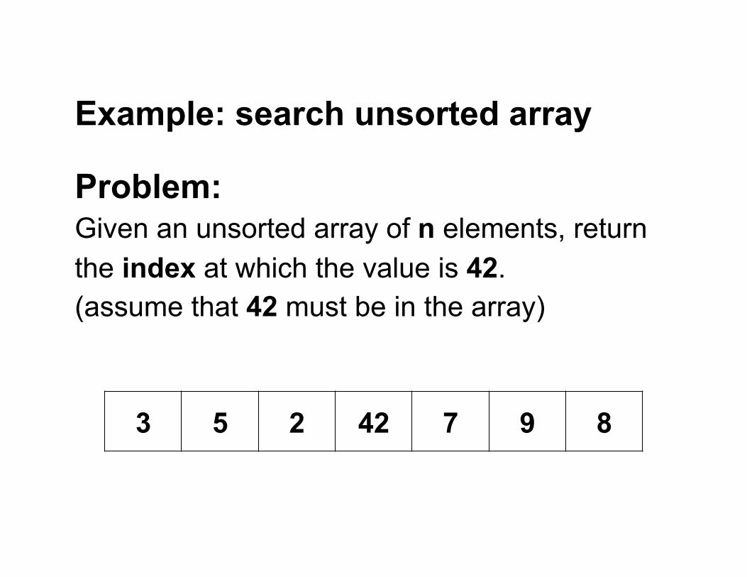
Example: search unsorted array

Problem: Given an unsorted array of n elements, return the index at which the value is 42. (assume that 42 must be in the array)

3 5 2 42 7 9 8

Possible algorithms

➔ Check through indices 1, 2, 3, …, n ➔ Check from n, n-1, n-2, …., to 1 ➔ Check all odd indices 1, 3, 5, …, then check

all even indices 2, 4, 6, … ➔ Check in the order 3, 1, 4, 1, 5, 9, 2, 6, ...

3 5 2 42 7 9 8

Prove: the lower bound on this problem is n-1, no matter what algorithm we use.

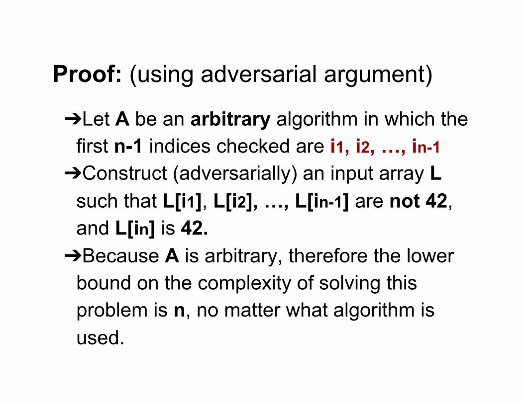
Proof: (using adversarial argument)

➔ Let A be an arbitrary algorithm in which the first n-1 indices checked are i1, i2, …, in-1

➔ Construct (adversarially) an input array L such that L[i1], L[i2], …, L[in-1] are not 42, and L[in] is 42.

➔ Because A is arbitrary, therefore the lower bound on the complexity of solving this problem is n, no matter what algorithm is used.

The problem

Given n elements, determine the maximum element. How many comparisons are needed at least?

The problem

Given n elements, determine the maximum element. How many comparisons are needed at least?

Answer: Need at least n-1 comparisons

Insight: upper bound for max How to design a maximum-finding algorithm that reaches the lower bound n-1 ?

➔ Make every comparison count, i.e., every comparison should guarantee to eliminate a possible candidate for maximum/champion.

➔  No match between losers, because neither of them is a candidate for champion.

➔  No match between a candidate and a loser, because if the candidate wins, the match makes no contribution (not eliminating a candidate)

These algorithms reach the lower bound

Linear scanning Tournament

Adversary strategy for Max Suppose Algorithm A claims to find the max of n elements using < n-1 comparisons (on some path)

Construct a graph in which we join two elements by an edge if they are compared (along this path) by A.

Since < n-1 comparisons on this path, the underlying graph has at least 2 components, C1 and C2

Suppose A outputs u in component C1 (as max)

Then we can fix values for elements in C1, C2 to be consistent with the comparisons, and where every element in C2 is larger than u. Contradiction!

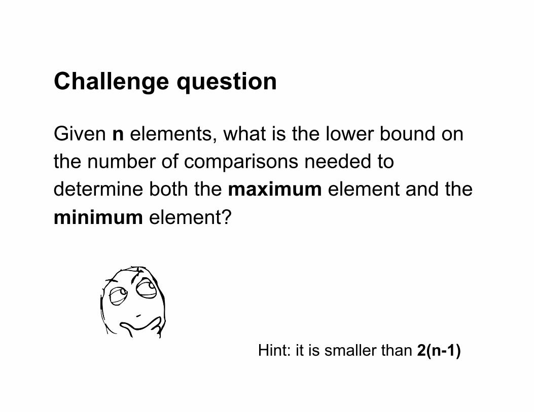
Challenge question

Given n elements, what is the lower bound on the number of comparisons needed to determine both the maximum element and the minimum element?

Hint: it is smaller than 2(n-1)

proving lower bounds using Reduction

The idea

➔ Proving one problem’s lower bound using another problem’s known lower bound.

➔ If we know problem B can be solved by solving an instance of problem A, i.e., A is “harder” than B

➔ and we know that B has lower bound L(n)

➔ then A must also be lower-bounded by L(n)

Example: Prove: ExtractMax on a binary heap is lower bounded by Ω(log n). Suppose ExtractMax can be done faster than log n, then HeapSort can be done faster than n log n, because HeapSort is basically ExtractMax n times But HeapSort, as a comparison based sorting algorithm, has been proven to be lower bounded by Ω(n log n). Contrdiction, so ExtractMax must be lower bounded by Ω(log n)

Final thoughts

what did we learn in CSC263

Data structures are the underlying skeleton of a good computer system. If you will get to design such a system yourself and make fundamental decisions, what you learned from CSC263 should give you some clues on what to do.

➔  Understand the nature of the system / problem, and model them into structured data

➔  Investigate the probability distribution of the input ➔  Investigate the real cost of operations ➔ Make reasonable assumptions and estimates where

necessary ➔  Decide what you care about in terms of performance,

and analyse it ◆  “No user shall experience a delay more than 500

milliseconds” -- worst-case analysis ◆ “It’s ok some rare operations take a long time” --

average-case analysis ◆ “what matter is how fast we can finish the whole

sequence of operations” -- amortized analysis

In CSC263, we learned to be a computer scientist,

not just a programmer.

Original words from lecture notes of Michelle Craig

what we did NOT learn but are now ready to learn

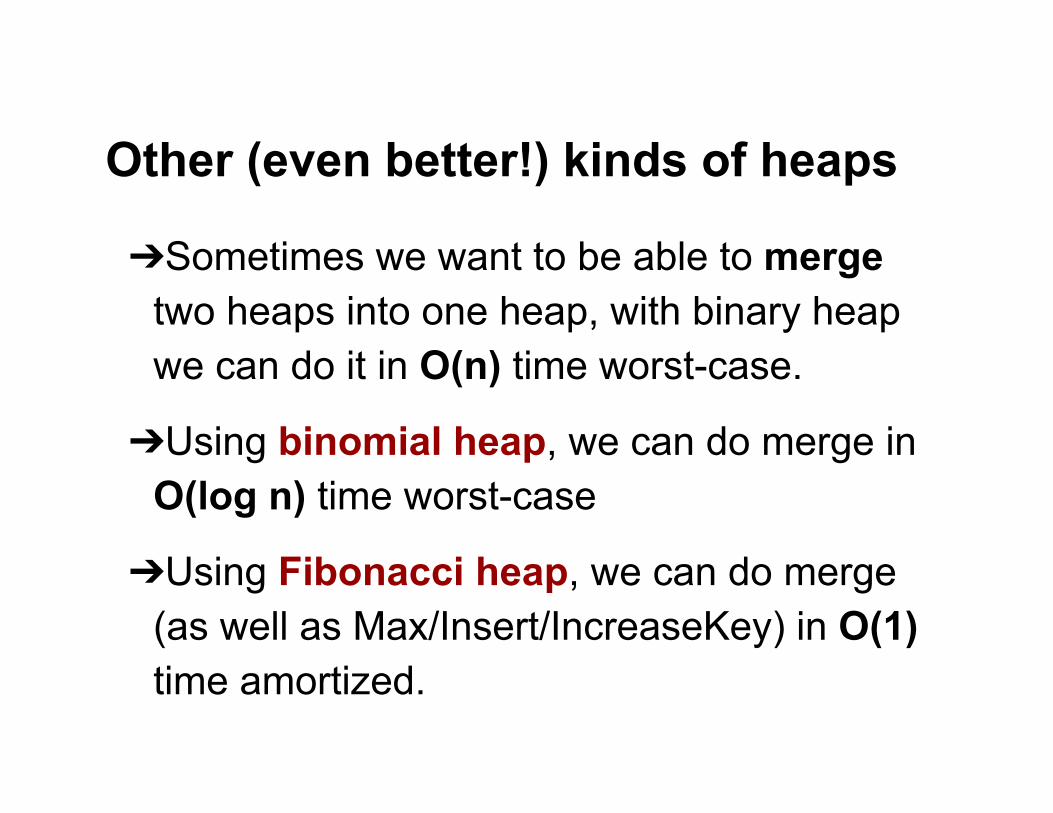
Other (even better!) kinds of heaps

➔ Sometimes we want to be able to merge two heaps into one heap, with binary heap we can do it in O(n) time worst-case.

➔ Using binomial heap, we can do merge in O(log n) time worst-case

➔ Using Fibonacci heap, we can do merge (as well as Max/Insert/IncreaseKey) in O(1) time amortized.

Even better kinds of search trees

➔ We learned BST and AVL tree, and there are others called red-black tree, 2-3 tree, splay tree, AA tree, scapegoat tree, etc.

➔ There is B-tree, optimized for accessing big blocks of data (like in a hard drive)

➔ There is B+ tree, which is even better than B-tree (widely used in database systems).

➔ You’ll learn about these in CSC443.

Amazing applications of hashing

➔ Perfect hashing guarantees worst-case

O(1) time for searching, instead of average-case O(1) time

➔ Cuckoo hashing (coolest thing ever)

Shortest paths in a graph

➔ We learned how to get shortest paths using BFS on a graph

➔ We did NOT learn how to get shortest

(weighted) paths on a weighted graph. ◆ Dijkstra, Bellman-Ford, ...

➔ You’ll learn about them in CSC 373

Greedy algorithms

➔ We learned that Kruskal’s and Prim’s MST algorithms are greedy

➔ What property is satisfied by the problems

that can be perfectly solved by greedy algorithms?

➔ Will learn in CSC373

Dynamic programming

➔ Pick an interesting algorithm design problem, very likely it involves dynamic programming

➔ Will learn in CSC373

P vs NP, approximation algorithms

➔ We learned a bit about lower bounds.

➔ There are some problems, we can prove they cannot be perfectly solved in polynomial time.

➔ For these problems, we have to design some approximation algorithms.

➔ Will learn in CSC373 / 463

As our circle of knowledge expands, so does the circumference of darkness surrounding it.

Final Exam Prep

Topics covered: all of them

➔ Heaps ➔ BST, AVL tree, augmentation ➔ Hashing ➔ Randomized algorithms, Quicksort ➔ Graphs, BFS, DFS, MST ➔ Disjoint sets ➔ Lower bounds ➔ Analysis: worst-case, average-case,

amortized.

Types of questions ➔  Short-answer questions testing basic understanding.

➔  Trace operations we learned on a data structure

➔  Implement an ADT using a data structure

➔  Analysis runtimes

◆ best / worst-case

◆ average-case

◆ amortized cost

➔ Given a real-world problem, design data structures / algorithms to solve it.

Study for the exam

➔ Review lecture notes/slides

➔ Review tutorial problems

➔ Review all problem sets / assignments

➔ Practice with past exams (available at

exam repository)

➔ Come to office hours whenever

confused.

Toni’s pre-exam office hours

➔ Monday Dec 7, 3-4pm

➔ Wednesday Dec 9, 1-2pm

Exam Time & Location

Friday, Dec 11, 2:00 - 5:00 pm

Go to the right location.

No aid sheet

All the best!