creo simulation live verification and benchmark cases€¦ · directions) applied on the...

Creo Simulation Live Verification

and Benchmark Cases

Verification Cases 3

1.0 Static Structural Analysis 3

1.1 Statically Indeterminate Reaction Force Analysis 3

1.2 Rectangular Plate with Circular Hole Subjected to Tensile Loading 4

1.3 Stepped Shaft in Axial Tension 5

1.4 Elongation of a Solid Bar 7

1.5 Laterally Loaded Tapered Beam 8

1.6 Circular Plate under Uniform Pressure 10

2.0 Modal Analysis 10

2.1 Cantilever Beam Modal Analysis 10

2.2 Simply-Supported Beam Modal Analysis 11

2.3 Modal Analysis of an Annular Plate 14

2.4 Modal Analysis of a Rectangular Plate 15

3.0 Thermal Analysis 15

3.1 Heat Transfer in a Composite Wall 15

3.2 Conduction in a Composite Solid Block 17

3.4 Heat Transfer from a Cooling Spine 18

Benchmark Cases 19

4.0 Benchmark Cases 19

4.1 Modal Analysis of a Robot Arm 19

4.2 Modal Analysis of a Printed Circuit Board 21

4.3 Static Loading of a Bracket 23

4.4 Static Loading of a Rocker Arm Assembly 25

4.5 Heat Transfer in a Package/Heat Sink Assembly 27

Verification Cases

1.0 Static Structural Analysis

1.1 Statically Indeterminate Reaction Force Analysis

An assembly of three prismatic bars is supported at both end faces and is axially loaded with

forces F1 and F2. Force F1 is applied on the face between Parts 2 and 3 and F2 is applied on the

face between Parts 1 and 2. Find reaction forces in the Y direction at the fixed supports. Reference: S. Timoshenko, Strength of Materials, Part 1, Elementary Theory and Problems, 3rd Edition, CBS Publishers and Distributors, pg. 22 and 26

Material Properties Geometric Properties Loading

E = 2.9008e7 psi Cross section of all parts = 1” x 1” Force F1 = -1000 (Y direction)

ν = 0.3 Length of Part 1 = 4" Force F2 = -500 (Y direction)

ρ = 0.28383 lbm/in3 Length of Part 2 = 3"

Length of Part 3 = 3”

Results Comparison for Discovery LIve (Quadro M2000M 4GB Graphics Card, Default Fidelity)

Results Target

Simulate Discovery

Live Simulate

live Percent Error*

Percent Difference

#

Y Reaction Force at Top Fixed Support (lbf) 900 900.164 899.4 899.4 0.067 0

Y Reaction Force at Bottom Fixed Support (lbf) 600

599.836 599.6 600.6 0.1 0.167

* Percentage difference between results and target value # Percentage difference in results from Discovery live and Simulate live

1.2 Rectangular Plate with Circular Hole Subjected to Tensile Loading

A rectangular plate with a circular hole is fixed along one of the end faces and a tensile

pressure load is applied on the opposite face. Find the Maximum Normal Stress in the x

direction on the cylindrical surfaces of the hole. Reference: J. E. Shigley, Mechanical Engineering Design, McGraw-Hill, 1st Edition, 1986, Table A-23, Figure A-23-1, pg. 673


E = 1000 Pa Length = 15 m Pressure = -100 Pa

ν = 0.0 Width = 5 m

Thickness = 1 m

Hole radius = 0.5 m


Results Target

Simulate

Discovery Live

Simulate live

Percent Error

Percent Difference

Maximum Normal X Stress (Pa)

312.5 313.272

296.65 281.8 9.81 4.99

Results Comparison for Discovery LIve (Quadro M2000M 4GB Graphics Card, Maximum Fidelity)

Results Target Discovery

Live Simulate live

Percent Error

Percent Difference

Maximum Normal X Stress (Pa) 312.5 337.8 300 4 11.19

1.3 Stepped Shaft in Axial Tension

Consider a stepped shaft under an applied axial load of 1000 psi on the smaller cross section of the

shaft, compute the stress concentration based on the fillet radius at the step as shown below:

Reference:Roark’s Formulas for Stress and Strain, Warren C. Young and Richard G. Budynas, 2002


E = 2.9008e7 psi D = 8 in Pressure = -1000 psi

ν = 0.3 h = 3 in

r = 1 in


Results Target

Simulate Discovery

Live Simulate

live Percent

Error Percent

Difference

Maximum Normal Y Stress (psi)

1376

1422.63

1497.6 1503 9.23 0.36

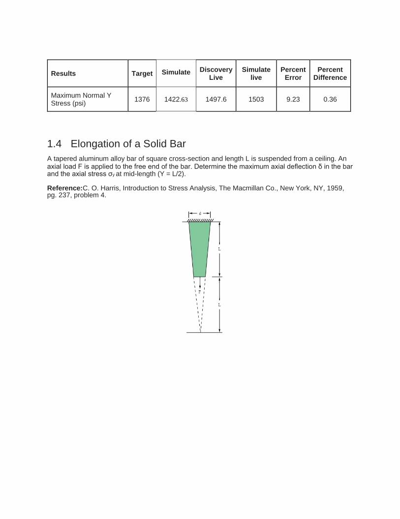
1.4 Elongation of a Solid Bar

A tapered aluminum alloy bar of square cross-section and length L is suspended from a ceiling. An axial load F is applied to the free end of the bar. Determine the maximum axial deflection δ in the bar and the axial stress σy at mid-length (Y = L/2). Reference:C. O. Harris, Introduction to Stress Analysis, The Macmillan Co., New York, NY, 1959, pg. 237, problem 4.


E = 10.4e6 psi L = 10 in F = 10000 lbf

ν = 0.3 d = 2 in

Results Comparison for Discovery Live (Quadro M2000M 4GB Graphics Card, Default Fidelity)

Results Target

Simulate Discovery

Live Simulate

live Percent

Error Percent

Difference

Directional Deformation Y (in)

0.0048077 0.0048156

0.004807 0.004807 0.015 0

Normal Stress Y at L/2 (psi)

4444 4439.45

4432

1.5 Laterally Loaded Tapered Beam

A cantilever beam of thickness t and length l has a depth which tapers uniformly from d at the tip to

3d at the wall. It is loaded by a force F at the tip, as shown. Find the maximum bending stress at the

mid-length and the fixed end of the beam. Reference: S. H. Crandall, N. C. Dahl, An Introduction to the Mechanics of Solids, McGraw-Hill Book Co., Inc., New York, NY, 1959, pg. 342, problem 7.18.


E = 30e6 psi l = 50 in F = 4000 lbf

ν = 0.0 d = 3 in

t = 2 in



Live Simulate

live Percent

Error Percent

Difference

Mid-Length Stress (psi) 8333 8229.5 -

Fixed End Stress (psi) 7407 - -

1.6 Circular Plate under Uniform Pressure

Consider a circular plate with fixed edges under a uniformly distributed pressure load. Find

the maximum deflection and bending stress in the center of the plate.

Reference: R. J. Roark, W. C. Young, Formulas for Stress and Strain, McGraw-Hill Book Co., Inc., New York, NY, 1975, Table 24.


E = 30e6 psi Diameter = 30 in P = 3 psi

ν = 0.3 Thickness = 0.25 in

Results Comparison for Discovery Live (Quadro M200M 4GB Graphics Card, Maximum Fidelity)

Results Target

Simulate Discovery

Live Simulate

live Percent

Error Percent

Difference

Deflection center of plate, in

0.0553 0.0549

0.0512 0.0512 7.41 0

Bending stress center of plate, psi

5265

Results Comparison for Discovery Live (8 GB Graphics Card, Max Fidelity)


Live Simulate

live Percent

Error Percent Error DL

Deflection center of plate, in 0.0553 0.0541 0.0531 3.97 1.84

Bending stress center of plate, psi 5265

2.0 Modal Analysis

2.1 Cantilever Beam Modal Analysis

Consider a cantilever beam of length l and a width w and height h. Compute the first three bending modes and natural frequencies. (Note that the simulation results include orthogonal bending, torsional and axial modes, and the results comparison compares the first three bending modes from a closed form solution with the equivalent simulation results.)

. Reference: W. T. Thompson, Theory of Vibration with Applications, 2nd Edition, Prentice-Hall, Inc., Englewood Cliffs, NJ, 1981, pg. 220

Material Properties Geometric Properties

E = 70e9 Pa l = 4 m

ν = 0.35 w = 0.346 m

⍴ = 2700 kg/m^3 h = 0.346 m

Results Comparison for Discovery Live (Quadro M200)M 4GB Graphics Card, Default Fidelity)

Results Target Simulate Discovery

Live Simulate live

Percent Error

Percent Difference

Frequency Mode 1 (Hz) 17.8 17.88 17.8 17.82 0.1 0.1

Frequency Mode 3 (Hz) 111.5 110.03 108 107.98 3.2 0.02

Frequency Mode 6 (Hz) 312.1 320.22 287 288.09 7.7 0.38

2.2 Simply-Supported Beam Modal Analysis Determine the fundamental frequency f of a simply-supported beam of length 80 in and

uniform cross-section A = 4 in2as shown below.

Reference: W. T. Thompson, Vibration Theory and Applications, 2nd Printing, Prentice-Hall, Inc., Englewood Cliffs, NJ, 1965, pg. 18, ex. 1.5-1


E = 3e7 psi l = 80 in

= 0.3 w = 2 in

⍴ = 0.2836 lb/in^3 h = 2 in

Results Comparison for Discovery Live (Quadro M2000M 4GB Graphics Card, Default Fidelity) (Simple support approximated by constraining 0.125 in imprinted faces.)

Results Target

Simulate Discovery

Live Simulate

live Percent

Error Percent

Difference

Frequency Mode 1 (Hz)

28.766 28.67

32.3 34.20 18.9 5.9

2.3 Modal Analysis of an Annular Plate

An assembly of three annular plates has cylindrical support (fixed in the radial, tangential, and axial

directions) applied on the cylindrical surface of the hole. Determine the first six natural frequencies. Reference:R. J. Blevins, Formula for Natural Frequency and Mode Shape, Van Nostrand Reinhold Company Inc., 1979, Table 11-2, Case 4, pg. 247


E = 2.9008e7 psi Inner diameter of inner plate = 20"

= 0.3 Inner diameter of middle plate = 28"

⍴ = 0.28383 lb/in^3 Inner diameter of outer plate = 34"

Outer diameter of outer plate = 40"

Thickness of all plates = 1"


Results Target

Simulate Discovery

Live Simulate

live Percent

Error Percent

Difference


310.9 310.92

321 321.5 3.41 0.16


318.1 316.37

326.6 327.2 2.86 0.18


318.1 316.50

326.7 327.2 2.86 0.15


351.6 347.80

358 358.6 1.99 0.17


351.6 347.94

358.1 358.6 1.99 0.14


442.4 436.54

446.5 447.3 1.11 0.18

2.4 Modal Analysis of a Rectangular Plate

Consider a rectangular plate with fixed supports where the dimensions of the plate are length = 6

in, width = 4 in and thickness = 0.063 in. Determine the natural frequency and mode shape.

Reference:R. Blevins, Formula for Natural Frequency and Mode Shape, Van Nostrand Reinhold Company Inc., 1979, Table 11-6


E = 1.0e7 psi Length = 6 in

= 0.33 Width = 4 in

⍴ = 0.1 lbm/in^3 Thickness = 0.063 in


Results Target

Simulate Discovery

Live Simulate

live Percent

Error Percent

Difference

Frequency Mode 1 (Hz) 1016 1019.35 1075.7 1075.7 5.88 0.00

3.0 Thermal Analysis

3.1 Heat Transfer in a Composite Wall A furnace wall consists of two layers: fire brick and insulating brick. The temperature inside the furnace is 3000°F (Tf) and the inner surface convection coefficient is 3.333 x 10-3 BTU/s ft2 °F (hf). The ambient temperature is 80°F (Ta) and the outer surface convection coefficient is 5.556 x 10-4 BTU/s ft2 °F (ha). Find the temperature distribution in the composite wall. Reference: F. Kreith, Principles of Heat Transfer, Harper and Row Publisher, 3rd Edition, 1976, Example 2-5, pg. 39


Fire brick: k = 2.222 x 10-4 BTU/s ft °F Insulation: k = 2.778 x 10-5BTU/s ft °F

Cross-section = 1” x 1” Fire brick thickness = 9” Insulating wall thickness = 5”


Results Target

Simulate

Discovery Live

Simulate live Percent

Error Percent

Difference

Minimum Temperature (°F) 336 336.64 326 333 0.89 2.15

Maximum Temperature (°F) 2957 2597.17 2964 2964 0.24 0.00

Convection:

Film coefficient:5.556 x 10 -4

BTU/s (ft2

)(°F) Ambient temperature: 80 °F

Convection:

Film coefficient:3.333 x 10-3

BTU/s (ft2)(°F)

Ambient temperature: 3000 °F

3.2 Conduction in a Composite Solid Block

Consider heat conduction in a wall formed as composite of two materials. Material one has a

uniform heat generation source equal to 6000 Watts applied to the outer surface, while

material two has an outer surface exposed to convective cooling. Compute the temperature of

the adiabatic surface on the left hand side of the domain.

Reference:F.P. Incropera, D.P. Dewitt. Fundamentals of Heat and Mass Transfer. 5th Edition, pg. 117, 2006.

Material Properties Geometric properties Loading

Material One: Dimensions of the block: Left surface: Heat flow = 6000 W

Conductivity = 75 W/m-K 70 mm X 80 mm Right surface: HTC = 1000 W/m2 K

Material Two: Material one = 50 mm and fluid bulk temperature = 30 C

Conductivity = 150 W/m-K Material two = 20 mm All other surfaces are adiabatic.

Thickness = 1000 mm


Results Target

Simulate

Discovery Live

Simulate live

Percent Error

Percent difference

Temperature of the adiabatic surface on extreme left side, C

165 165

162.7 162.7 1.40 0

3.3 Heat Transfer from a Cooling Spine

A steel cooling spine of cross-sectional area A and length L extend from a wall that is maintained at temperature T w . The surface convection coefficient between the spine and the surrounding air is h, the air temper is T a , and the tip of the spine is insulated. Find the heat conducted by the spine and the temperature of the tip.

Reference:F. Kreith, "Principles of Heat Transfer", 2nd Printing, International Textbook Co., Scranton, PA, 1959, pg. 143, ex. 4-5.


K = 9.71x10-3 BTU/s-ft-°F

Cross section = 1.2 in x 1.2 in L = 8 in

T w = 100 °F T a = 0 °F H = 2.778x10-4 BTU/s-ft2-°F

Results Comparison for Discovery Live (4GB Graphics Card, Default Fidelity)

Results Target

Simulate

Discovery Live

Simulate live Percent

Error Percent

Difference

Temperature of Tip, °F

79.0344 78.96

79.026 79.024 0.01 0.00

Benchmark Cases

4.0 Benchmark Cases

4.1 Modal Analysis of a Robot Arm

Consider a steel robot arm assembly with a fixed base. Calculate the first three natural frequencies

and mode shapes of the assembly.

Material Properties Boundary Conditions

Young’s modulus = 2e11 Pa Fixed support

Poisson’s ratio = 0.3

Creo Simulate Live Mode 2

Results Discovery

Live Simulate

live Percent

difference

Mode 1 Frequency, Hz 18.4 18.4 0.0



Quadro P4000, maximum fidelity

Below is the convergence of Mode 1 vs the resolution size:

Results (default fidelity P4000) Discovery

Live Simulate

live Percent

difference




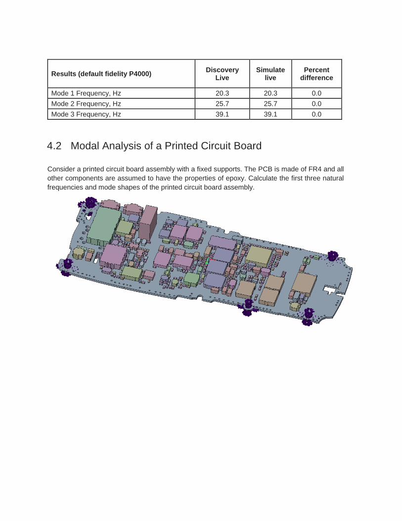
4.2 Modal Analysis of a Printed Circuit Board

Consider a printed circuit board assembly with a fixed supports. The PCB is made of FR4 and all

other components are assumed to have the properties of epoxy. Calculate the first three natural

frequencies and mode shapes of the printed circuit board assembly.

Printed Circuit Board Assembly


FR4 Fixed support on five support holes as shown Young’s modulus = 1.1e10 Pa

Density = 1900 kg/m3

Poisson’s ratio = 0.28 Epoxy

Young’s modulus = 1.1e9 Pa

Density = 950 kg/m

Poisson’s ratio = 0.42

Creo Simulate Live Mode 1

Live, Quadro P4000, maximum fidelity

Results Discovery

Live Simulate

live Percent

difference



Mode 3 Frequency, Hz 836 836.091 0.01

Below is the convergence of Mode 1 vs the resolution size:

Results (default fidelity P4000) Discovery

Live Simulate

live Percent

difference




4.3 Static Loading of a Bracket

Consider the static loading of an aluminum bracket. The loading consists of an applied load of 200

N and two fixed supports. Calculate the maximum tip displacement and maximum equivalent stress

in the rear cut-out of the part as a function of the position of the Fidelity slider in both Discovery Live

and Discovery AIM.

Static Loading of a Bracket

Creo Simulate Live Equivalent Stress (Max Fidelity)

Quadro P4000

Fidelity Slider Position (Percentage)

Discovery Live Displacement m

Simulate Live Displacement m

Percent difference

Percent Error Simulate Live 100% Fidelity

0 1.135E-04 1.107E-04 0.025 0.006

25 1.101E-04 1.103E-04 0.001 0.001

50 1.101E-04 1.100E-04 0.001 0.001

75 1.103E-04 1.101E-04 0.002 0.000

100 1.102E-04 1.101E-04 0.001 0.000

Fidelity Slider Position (Percentage)

Discovery Live Stress MPa

Simulate Live Stress MPa

Percent difference

Percent Error Simulate Live 100% Fidelity

0 16.14 16.22 0.005 0.163

25 18.01 17.25 0.044 0.110

50 17.93 17.74 0.011 0.085

75 19.41 19.16 0.013 0.011

100 18.25 19.38 0.058 0.000

4.4 Static Loading of a Rocker Arm Assembly

Consider the static loading of a rocker arm assembly with variable fillet radii. The loading consists of

an applied load of 600 N, a frictionless and a fixed support. Calculate the maximum equivalent

stress.

Creo Simulate Live Equivalent Stress, Radii = 3 mm

Quadro P4000, Maximum Fidelity

Discovery Live Stress MPa


Percent difference

132.3 130.04 1.7

4.5 Heat Transfer in a Package/Heat Sink Assembly

Consider the steady-state heat transfer of an aluminum heat sink, thermal interface layer and

package assembly. The package generates 5 Watts of power and the outer surfaces of the heat

sink have a convection boundary condition with a heat transfer coefficient of 5 W/m^2 °C and fluid

bulk temperature of 20 °C. Calculate the maximum temperature in the aluminum heat sink and the

maximum temperature in the assembly for a steady-state condition.


Aluminum, K = 148.62 W/m °C Package Heat Flow = 5 W

TIM, K = 24 W/m °C Heat Transfer Coefficient = 5 W/m^2 °C

Package, K = 2 W/m °C Fluid Bulk Temperature = 20 °C

Live temperature in heat sink/package assembly

Live, Quadro P4000 default fidelity

Results: Default Fidelity Discovery Live Stress MPa


Percent difference

Max Temperature Heat Sink, °C 43.3 43.85 1.3

Max Temperature, °C 52.5 52.48 0.04

Results: Maximum Fidelity Discovery Live

Simulate Live

Percent difference

Max Temperature Heat Sink, °C 42.908 42.45 1.1

Max Temperature, °C 52.523 51.25 2.4

creo simulation live verification and benchmark cases€¦ · directions) applied on the...

Documents