Coules, H., & Smith, D. (2015). The maximum possible stress intensityfactor for a crack in an unknown residual stress field. International Journal ofPressure Vessels and Piping, 134, 33-45.

Peer reviewed version

Link to publication record in Explore Bristol ResearchPDF-document

University of Bristol - Explore Bristol ResearchGeneral rights

This document is made available in accordance with publisher policies. Please cite only the publishedversion using the reference above. Full terms of use are available:http://www.bristol.ac.uk/pure/about/ebr-terms

Take down policy

Explore Bristol Research is a digital archive and the intention is that deposited content should not beremoved. However, if you believe that this version of the work breaches copyright law please contactopen-access@bristol.ac.uk and include the following information in your message:

• Your contact details• Bibliographic details for the item, including a URL• An outline of the nature of the complaint

On receipt of your message the Open Access Team will immediately investigate your claim, make aninitial judgement of the validity of the claim and, where appropriate, withdraw the item in questionfrom public view.

The maximum possible stress intensity factor for a crack in an

unknown residual stress field

H. E. Coules* and D. J. Smith

Department of Mechanical Engineering, University of Bristol, Bristol, BS8 1TR, UK

*Corresponding author.

Email: harry.coules@bristol.ac.uk

Telephone: +44 (0)117 331 5941

Abstract Residual and thermal stress fields in engineering components can act on cracks and structural flaws,

promoting or inhibiting fracture. However, these stresses are limited in magnitude by the ability of

materials to sustain them elastically. As a consequence, the stress intensity factor which can be

applied to a given defect by a self-equilibrating stress field is also limited. We propose a simple

weight function method for determining the maximum stress intensity factor which can occur for a

given crack or defect in a one-dimensional self-equilibrating stress field, i.e. an upper bound for the

residual stress contribution to 𝐾𝐼. This can be used for analysing structures containing defects and

subject to residual stress without any information about the actual stress field which exists in the

structure being analysed. A number of examples are given, including long radial cracks and fully-

circumferential cracks in thick-walled hollow cylinders containing self-equilibrating stresses.

Keywords: Residual stress, fracture, weight function, stress intensity factor, upper bound.

Highlights An upper limit to the contribution of residual stress to stress intensity factor

The maximum 𝐾𝐼 for self-equilibrating stresses in several geometries is calculated

A weight function method can determine this maximum for 1-dimensional stress fields

Simple MATLAB scripts for calculating maximum 𝐾𝐼 provided as supplementary material

Nomenclature 𝑎 Crack length

𝑎𝑡 Crack length below which a uniformly tensile stress of magnitude 𝜎𝑙𝑖𝑚 in the direction normal to the crack can exist over the entire length of the prospective crack in a self-equilibrating stress distribution

𝐴 Total sectional area

𝑏 Overall section width or characteristic length

𝑐 Distance of a point force from the crack mouth (or from the centre of a symmetric crack)

𝐾𝐼 Mode I stress intensity factor

𝐾𝐼𝑚𝑎𝑥 Maximum possible Mode I stress intensity factor which can be generated by a

residual stress

𝑚 Weight function for 𝐾𝐼 for unit normal crack face point loading

𝑚𝑙𝑖𝑚 Limiting value of the weight function used for assigning tensile and compressive stress regions

(𝑛𝑘) Sequence of indices of the largest elements of 𝑚(𝑥𝑛)

𝑟(𝑥𝑛)

𝑃 Normal point force applied to crack face(s)

𝑞 Welding torch power

𝑄 Weld heat input per unit length per unit section thickness

𝑟 Radial distance (cylindrical coordinates)

𝑟𝑎 Radius from the axis of the pipe to the tip of a circumferential crack

𝑟𝑖 Pipe internal radius

𝑟𝑜 Pipe external radius

𝑣 Velocity of welding torch

𝑥 Distance in crack extension direction (Cartesian coordinates)

𝑥𝑛 Set of 𝑁 uniformly-spaced points in the interval 0 ≤ 𝑥 ≤ 𝑎

𝑦 Distance in the direction normal to the crack plane (Cartesian coordinates)

𝑧 Axial distance (cylindrical coordinates)

𝜃 Azimuth (cylindrical coordinates)

𝜎𝑏 Bending component of a sectional residual stress distribution

𝜎𝑚 Membrane component of a sectional residual stress distribution

𝜎𝑙𝑖𝑚 Maximum possible stress in the direction normal to the crack plane

𝜎𝑠𝑒 Self-equilibrating component of a sectional residual stress distribution

𝕏𝑐 Domain of compressive crack-normal stress on the prospective crack plane

𝕏𝑡 Domain of tensile crack-normal stress on the prospective crack plane

1. Introduction Residual stresses strongly influence elastic fracture, but can be difficult and time-consuming to

measure [1]. Furthermore, accurate prediction of the residual stresses which result from

manufacturing operations is challenging and usually involves the use of elastic-plastic finite element

modelling. As a consequence, fracture-mechanics-based integrity assessment of components and

structures containing residual stresses is often hampered by a lack of reliable residual stress data for

the object being analysed [2]. When the residual stress distribution is not known, it is necessary to

use conservative assumptions regarding the nature of the residual stress field. This results in

cautious and often highly conservative assessments of structural integrity for residual stress-bearing

structures, often leading to safe plant being taken out of service earlier than required and at

significant cost.

The most important way in which residual stress information is used in the assessment of structural

integrity is to calculate the contribution of the residual stress state to the Mode I stress intensity

factor 𝐾𝐼 for a given defect in the component or structure being assessed. In the absence of residual

stress data, most structural integrity assessment procedures such as BS7910 [3] and R6 [4] specify

that a conservative estimate of the residual stress state should be used. This can be taken from a

handbook of distributions which provide an upper bound to previous experimental data for common

geometries. In cases for which such bounding distributions are not available, it is often assumed that

the crack-normal stress is uniformly tensile and at yield magnitude [5]. The use of conservative

estimates of the real residual stress distribution in a component simplifies analysis but can lead to

unrealistically large estimates of 𝐾𝐼, especially for deeper cracks and defects. The fundamental issue

is that conservative estimates of the residual stress distribution must be biased towards a tensile

state of crack-normal stress. However, for deeper cracks the effect of this tensile bias on the

resulting calculated stress intensity factor can become very large, resulting in estimates of the

residual stress contribution to 𝐾𝐼 which are unrealistically high.

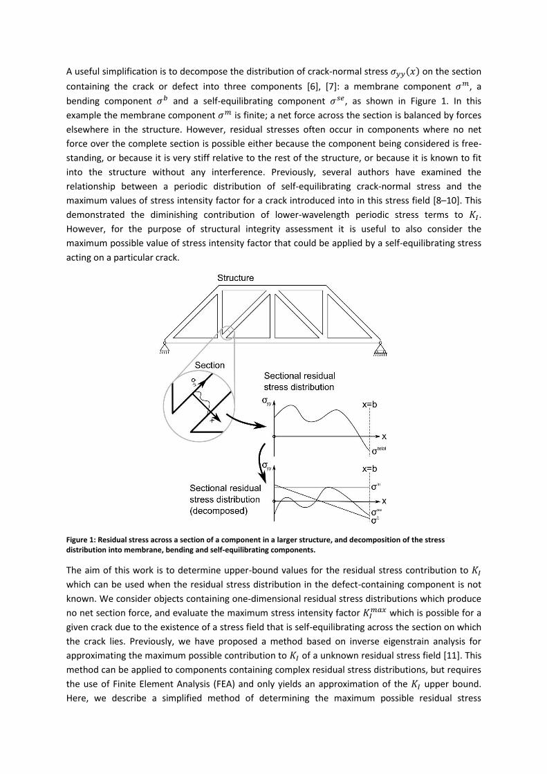
A useful simplification is to decompose the distribution of crack-normal stress 𝜎𝑦𝑦(𝑥) on the section

containing the crack or defect into three components [6], [7]: a membrane component 𝜎𝑚, a

bending component 𝜎𝑏 and a self-equilibrating component 𝜎𝑠𝑒, as shown in Figure 1. In this

example the membrane component 𝜎𝑚 is finite; a net force across the section is balanced by forces

elsewhere in the structure. However, residual stresses often occur in components where no net

force over the complete section is possible either because the component being considered is free-

standing, or because it is very stiff relative to the rest of the structure, or because it is known to fit

into the structure without any interference. Previously, several authors have examined the

relationship between a periodic distribution of self-equilibrating crack-normal stress and the

maximum values of stress intensity factor for a crack introduced into in this stress field [8–10]. This

demonstrated the diminishing contribution of lower-wavelength periodic stress terms to 𝐾𝐼.

However, for the purpose of structural integrity assessment it is useful to also consider the

maximum possible value of stress intensity factor that could be applied by a self-equilibrating stress

acting on a particular crack.

Figure 1: Residual stress across a section of a component in a larger structure, and decomposition of the stress distribution into membrane, bending and self-equilibrating components.

The aim of this work is to determine upper-bound values for the residual stress contribution to 𝐾𝐼

which can be used when the residual stress distribution in the defect-containing component is not

known. We consider objects containing one-dimensional residual stress distributions which produce

no net section force, and evaluate the maximum stress intensity factor 𝐾𝐼𝑚𝑎𝑥 which is possible for a

given crack due to the existence of a stress field that is self-equilibrating across the section on which

the crack lies. Previously, we have proposed a method based on inverse eigenstrain analysis for

approximating the maximum possible contribution to 𝐾𝐼 of a unknown residual stress field [11]. This

method can be applied to components containing complex residual stress distributions, but requires

the use of Finite Element Analysis (FEA) and only yields an approximation of the 𝐾𝐼 upper bound.

Here, we describe a simplified method of determining the maximum possible residual stress

contribution to 𝐾𝐼 which is applicable to one-dimensional stress distributions with 𝜎𝑚 = 0. This

method is based on weight function analysis, so for many geometries it can be performed using

existing weight function solutions without the need for additional FEA results.

2. Method of analysis

2.1 Force and moment equilibrium

Figure 1 shows the (one-dimensional) distribution of residual stress inside a component which forms

part of a larger structure, and how it can be decomposed into membrane (𝜎𝑚), bending (𝜎𝑏) and

self-equilibrating (𝜎𝑠𝑒) parts. For a finite membrane stress to occur, the rest of the structure must

impart a force on the component, i.e. the component must only fit into the structure with

interference. Likewise, for the stress distribution shown in Figure 1 a finite bending component can

only occur if the rest of the structure imparts a bending moment. In this situation, the component is

said to be in global bending [9]. This is shown in Figure 2a with the example of a plate containing a

self-equilibrating stress combined with an external moment, but in this case no membrane stress.

a.

b.

c.

Figure 2: a.) Residual stress distribution in a plate subject to bending. b.) Axisymmetric distribution of residual stress with both through-wall bending and self-equilibrating components in a pipe. c.) Residual stress on a radial plane of a pipe.

Some components contain residual stress distributions which are symmetric about a neutral axis of

their section. These symmetric stress distributions can contain an apparent bending component

which, due to the symmetry of the stress field, can exist in the absence of an externally-applied

moment. This is known as ‘local’ or ‘through-wall’ bending and is shown in Figure 2b. Residual stress

distributions of this type, which are symmetric on a plane, are found in many components of

practical importance such as autofrettaged tubes, seamless pipes, circumferentially-welded pipes

and toughened glass panels in which the residual stress profile is symmetric about the mid-plane.

The method described in this article is applicable to these cases, where the residual stress

distribution may contain finite self-equilibrating and through-wall bending components but where

there is no membrane stress or global bending. Another important case that the method can be

applied to is shown in Figure 2c: here the residual stress is invariant over the length of the

component, but is not (necessarily) axisymmetric. On any radial plane, such as the one shown, 𝜎𝑚 =

0 due the requirement for moment equilibrium about the pipe axis, but a through-wall bending

stress is still possible. This form of residual stress distribution is common in longitudinally-welded

pipes. When applied to a component in which the stress distribution is not symmetric about a

neutral axis (such as in Figure 1a), the method described here determines the maximum stress

intensity factor that can occur under any combination of self-equilibrating and bending stress (which

does not exceed 𝜎𝑙𝑖𝑚 - see Equation 3), in the absence of any membrane stress.

The condition for zero membrane stress is:

Equation 1

𝜎𝑚 =1

𝐴∫ 𝜎𝑦𝑦𝐴

𝑑𝐴 = 0

Where 𝐴 is the area of the section. For a distribution of stress on a section which varies in one

Cartesian dimension (𝑥) only, this reduces to:

Equation 2

𝜎𝑚 =1

𝑏∫ 𝜎𝑦𝑦(𝑥)𝑏

0

𝑑𝑥 = 0

where 𝑏 is the section width as shown in Figure 1. The equivalent expression for axisymmetric

distributions of stress is discussed in Section 2.4. Since real residual stress fields cannot have an

infinite magnitude, it can be assumed that there is some maximum value of 𝜎𝑦𝑦 (denoted 𝜎𝑙𝑖𝑚)

which is not exceeded anywhere on a given plane in either tension or compression:

Equation 3

|𝜎𝑦𝑦| ≤ 𝜎𝑙𝑖𝑚

Given the conditions imposed by Equation 2 and Equation 3, consider a crack of length 𝑎 ≤ 𝑏 2⁄

introduced into a stress field which varies in one Cartesian direction only and which is symmetric

about the neutral axis of the section. The example of a centre-cracked plate is shown in Figure 3a.

The stress distribution in Figure 3b cannot be supported due to the condition imposed by Equation

2; it would require an externally-applied tensile force. By contrast, the stress distribution shown in

Figure 3c does satisfy Equation 2 and it results in the same value of 𝐾𝐼 due to identical loading of the

prospective crack line. However, for a crack of length 𝑎 > 𝑏 2⁄ it is not possible to support a stress of

𝜎𝑦𝑦 = +𝜎𝑙𝑖𝑚 over the entire crack length while satisfying Equation 2. The remaining section width

𝑏 − 𝑎 is insufficient to support the required force. This poses the question: what is the self-

equilibrating distribution of stress in the interval 0 ≤ 𝑥 ≤ 𝑏 that produces the maximum possible

stress intensity factor for deeper cracks?

a.

b.

c.

Figure 3: A centre-cracked plate subject to different distributions of stress which are symmetric about 𝒙 = 𝟎. a.) Centre-

cracked plate geometry. b.) Uniform applied stress of magnitude 𝝈𝒍𝒊𝒎. c.) Self-equilibrating stress distribution that has a

magnitude 𝝈𝒍𝒊𝒎 over the prospective crack line - this can only be sustained if 𝒂 ≤ 𝒃 𝟐⁄ .

2.2 Deeper cracks

To determine the stress intensity factor due to an arbitrary stress distribution on the crack plane it is

possible to integrate the results for point loading at different distances along the crack face (the

weight function method [12], [13]). 𝐾𝐼 is given by [14]:

Equation 4

𝐾𝐼 = ∫ 𝑚(𝑎, 𝑏, 𝑐)𝜎𝑦𝑦(𝑐) 𝑑𝑐𝑎

0

Where 𝑚 is the weight function for the Mode I stress intensity factor due to a unit crack-opening

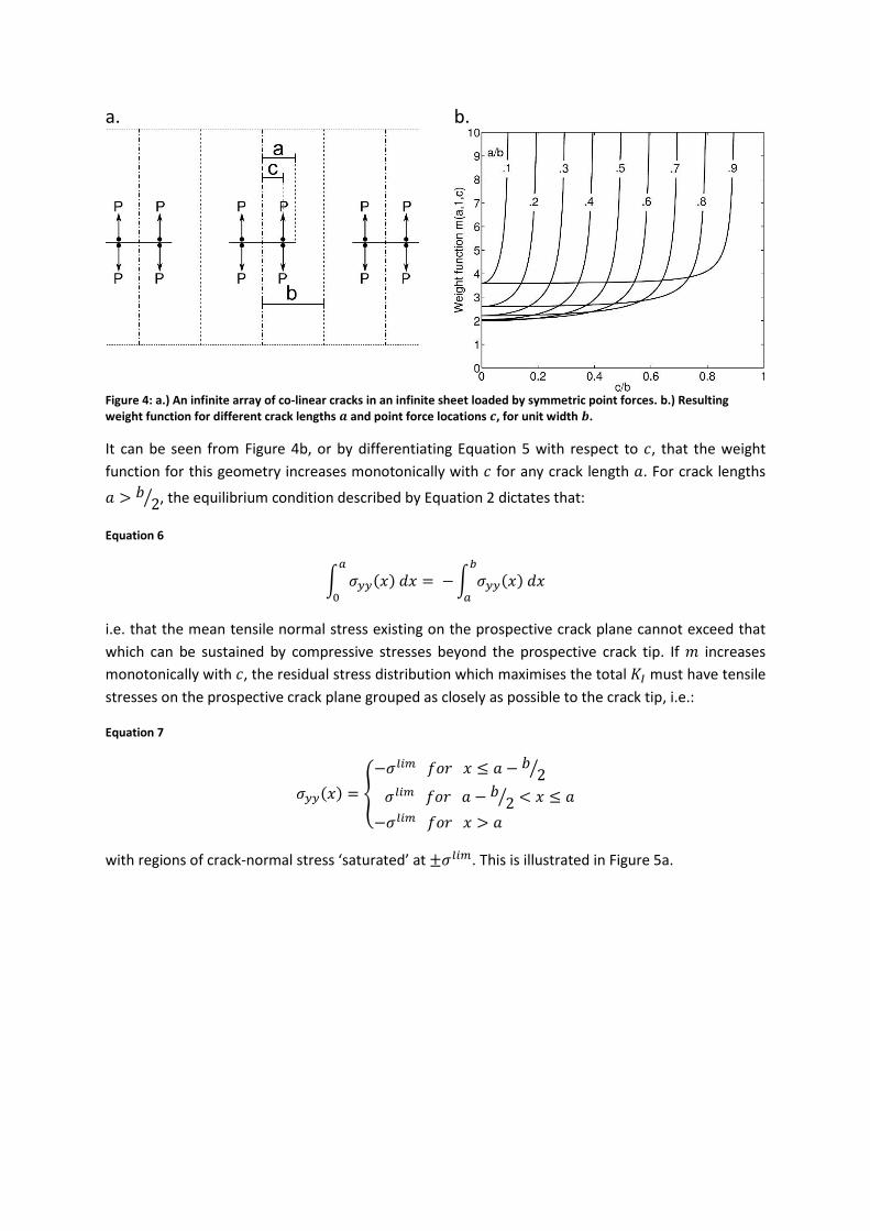
point force at a distance 𝑐 along the crack face. Figure 4a shows an infinite array of co-linear cracks

in an infinite plane body, loaded by a set of point forces of magnitude 𝑃. In this instance the weight

function is, exactly [14], [15]:

Equation 5

𝑚(𝑎, 𝑏, 𝑐) =1

𝑏√2𝑏 tan

𝜋𝑎

2𝑏

cos𝜋𝑐2𝑏

√(sin𝜋𝑎2𝑏)2− (sin

𝜋𝑐2𝑏)2

for unit 𝑃. This is shown in Figure 4b.

a.

b.

Figure 4: a.) An infinite array of co-linear cracks in an infinite sheet loaded by symmetric point forces. b.) Resulting weight function for different crack lengths 𝒂 and point force locations 𝒄, for unit width 𝒃.

It can be seen from Figure 4b, or by differentiating Equation 5 with respect to 𝑐, that the weight

function for this geometry increases monotonically with 𝑐 for any crack length 𝑎. For crack lengths

𝑎 > 𝑏 2⁄ , the equilibrium condition described by Equation 2 dictates that:

Equation 6

∫ 𝜎𝑦𝑦(𝑥) 𝑑𝑥 = −∫ 𝜎𝑦𝑦(𝑥) 𝑑𝑥𝑏

𝑎

𝑎

0

i.e. that the mean tensile normal stress existing on the prospective crack plane cannot exceed that

which can be sustained by compressive stresses beyond the prospective crack tip. If 𝑚 increases

monotonically with 𝑐, the residual stress distribution which maximises the total 𝐾𝐼 must have tensile

stresses on the prospective crack plane grouped as closely as possible to the crack tip, i.e.:

Equation 7

𝜎𝑦𝑦(𝑥) = {

−𝜎𝑙𝑖𝑚 𝑓𝑜𝑟 𝑥 ≤ 𝑎 − 𝑏 2⁄

𝜎𝑙𝑖𝑚 𝑓𝑜𝑟 𝑎 − 𝑏 2⁄ < 𝑥 ≤ 𝑎

−𝜎𝑙𝑖𝑚 𝑓𝑜𝑟 𝑥 > 𝑎

with regions of crack-normal stress ‘saturated’ at ±𝜎𝑙𝑖𝑚. This is illustrated in Figure 5a.

a.

b.

Figure 5: 𝑲𝑰-maximising residual stress field for a n infinite array of co-linear cracks of length 𝒂 > 𝒃 𝟐⁄ . a.) Stress field for

a single half-period, b.) stress field imposed on the array of cracks.

Substituting Equation 7 and Equation 5 into Equation 4 and integrating, we get the maximum 𝐾𝐼 that

can be generated in this crack geometry by a self-equilibrating one-dimensional distribution of

stress, as a function of crack length 𝑎:

Equation 8

𝐾𝐼𝑚𝑎𝑥(𝑎) =

{

𝜎𝑙𝑖𝑚√2𝑏 tan

𝜋𝑎

2𝑏 𝑓𝑜𝑟 𝑎 ≤ 𝑏 2⁄

𝜎𝑙𝑖𝑚√2𝑏 tan𝜋𝑎

2𝑏

[

1 −4

𝜋sin−1

(

sin

𝜋(𝑎 − 𝑏 2⁄ )

2𝑏

sin𝜋𝑎2𝑏

)

]

𝑓𝑜𝑟 𝑎 > 𝑏 2⁄

2.3 Non-monotonic weight functions

In geometries for which the weight function does not increase monotonically with 𝑐, the residual

stress distribution described by Equation 7 will not necessarily maximise 𝐾𝐼 for all crack lengths in

the range 𝑏 2⁄ < 𝑎 < 𝑏. In such cases, the 𝐾𝐼-maximising distribution of residual stress across the

prospective crack plane can be found using the following method.

Since a uniform compressive crack-normal stress −𝜎𝑙𝑖𝑚 can be sustained by the part of the section

beyond the crack, tensile and compressive stress regions must occur in the ratio 𝑏 2⁄ ∶ 𝑎 − 𝑏 2⁄ over

the crack length in the residual stress distribution which maximises 𝐾𝐼. The domains over which

tensile and compressive stresses occur can be found using the weight function for the crack length

of interest. An example is shown in Figure 6: a centre-cracked plate (or plane strain bar) of finite

width 𝑏 and length ℎ containing a distribution of stress which is symmetric about the plate

centreline (𝑥 = 0). No external forces or constraints act on the plate.

a.

b.

c.

d.

Figure 6: Determining the 𝑲𝑰-maximising distribution of residual stress for a centre-cracked plate of finite length and width. a.) Crack geometry, b.) weight functions for various crack lengths for unit width 𝒃, c.) assigning tensile and compressive domains using the weight function for a crack of length 𝟎. 𝟕𝒃, d.) resulting 𝑲𝑰-maximising distribution of crack-normal stress for 𝒂 = 𝟎. 𝟕𝒃.

The weight function for cracks of length 0 ≤ 𝑎 ≤ 0.7𝑏 in this geometry is shown in Figure 6b [16].

This weight function does not always increase monotonically with 𝑐. In a 𝐾𝐼-maximising residual

stress distribution, the domains over which tensile and compressive crack-normal stress occur are,

respectively:

Equation 9

𝕏𝑡 = {𝑥 | 𝑚(𝑎, 𝑏, 𝑥) ≥ 𝑚𝑙𝑖𝑚 , 0 ≤ 𝑥 < 𝑎}

𝕏𝑐 = {𝑥 | 𝑚(𝑎, 𝑏, 𝑥) < 𝑚𝑙𝑖𝑚 , 0 ≤ 𝑥 < 𝑎}

where 𝑚𝑙𝑖𝑚 is a limiting value of the weight function which separates these two domains. This

limiting value can be determined numerically by taking 𝑁 uniformly spaced locations 𝑥𝑛 over the

domain 0 ≤ 𝑥 ≤ 𝑎, and evaluating 𝑚 at each location. 𝑚𝑙𝑖𝑚 is then equal to the 𝑁𝑏

2𝑎’th largest value

of 𝑚(𝑎, 𝑥𝑛) in the limit 𝑁 → ∞. Once the tensile and compressive domains have been assigned using

Equation 9, the maximum stress intensity factor for this geometry is evaluated as:

Equation 10

𝐾𝐼𝑚𝑎𝑥(𝑎) = 𝜎𝑙𝑖𝑚 [ ∫ 𝑚(𝑎, 𝑏, 𝑥) 𝑑𝑥

𝕏𝑡

− ∫ 𝑚(𝑎, 𝑏, 𝑥) 𝑑𝑥

𝕏𝑐

]

For a crack of length 𝑎

𝑏= 0.7 in a centre cracked plate of length ℎ = 0.8𝑏 with unit width 𝑏 as shown

in Figure 6a, 𝑚𝑙𝑖𝑚 = 3.717 (see Figure 6c). Using 𝑚𝑙𝑖𝑚, the maximum Mode 1 stress intensity factor

can be calculated via Equation 9 and Equation 10. In normalised form it is: 𝐾𝐼𝑚𝑎𝑥

𝜎𝑙𝑖𝑚√𝜋𝑏= 0.793.

2.4 Axisymmetric cracks

A similar procedure to that described in Section 2.3 may be used for axisymmetric cracks. For

example, Figure 7 shows thick-walled pipes containing surface-breaking circumferential cracks. For

any self-equilibrating stress distribution in such pipes prior to cracking, forces in the axial direction

must sum to zero, i.e.:

Equation 11

∫ 2𝜋𝑟. 𝜎𝑧𝑧(𝑟) 𝑑𝑟 = 0𝑟𝑜

𝑟𝑖

where 𝑟 is the radial coordinate, and 𝑟𝑖 and 𝑟𝑜 are the inner and outer radii of the pipe wall

respectively. For circumferential cracks, the crack length below which a tensile stress of magnitude

𝜎𝑙𝑖𝑚 can be sustained across the entire prospective crack face by a self-equilibrating stress field will

be denoted 𝑎𝑡. For planar objects this was simply equal to 𝑏

2.

a.

b.

c.

d.

Figure 7: Thick-walled hollow cylinders containing circumferential cracks: a,b.) internal crack, c,d.) external crack.

By considering equal sectional areas for the crack and the un-cracked ligament of pipe wall, 𝑎𝑡 can

be calculated as:

Equation 12

𝑎𝑡 = 𝑟𝑜√1

2(𝑟𝑖2

𝑟𝑜2 + 1) − 𝑟𝑖

for an internal crack, and:

Equation 13

𝑎𝑡 = 𝑟𝑜 [1 − √1

2(𝑟𝑖2

𝑟𝑜2 + 1)]

for an external crack. For this type of geometry 𝑎𝑡 always lies between the limits (1 −1

√2)𝑏 (an

external crack in a solid cylinder) and 𝑏

√2 (a penny-shaped internal crack in a solid cylinder). In these

two limiting cases 𝑏 represents the radius of the solid cylinder, since 𝑟𝑖 → 0.

For the planar cracks described in Sections 2.2 and 2.3, the tensile and compressive regions of the

𝐾𝐼-maximising residual stress field for crack lengths 𝑎 > 𝑎𝑡 were assigned using a limiting value of

the weight function (see Equation 9). For axisymmetric cracks, the overall force applied to the

section due to a line force of unit magnitude varies with radius due the differing circumference of

the line over which the force acts. Therefore, to determine the maximum stress intensity factor that

can be achieved for zero net section force, the weight function normalised by 𝑟 must be used.

Equation 9 becomes:

Equation 14

𝕏𝑡 = {𝑥 | 𝑚(𝑥)

𝑟(𝑥)≥ (

𝑚

𝑟)𝑙𝑖𝑚

, 0 ≤ 𝑥 < 𝑎}

𝕏𝑐 = {𝑥 | 𝑚(𝑟)

𝑟(𝑥)< (

𝑚

𝑟)𝑙𝑖𝑚

, 0 ≤ 𝑥 < 𝑎}

where (𝑚

𝑟)𝑙𝑖𝑚 is the limiting value of

𝑚

𝑟. The radius as a function of the 𝑥-coordinate, 𝑟(𝑥), is:

Equation 15

𝑟(𝑥) = 𝑟𝑖 + 𝑥

for internal cracks, and:

Equation 16

𝑟(𝑥) = 𝑟𝑜 − 𝑥

for external cracks. The limiting value (𝑚

𝑟)𝑙𝑖𝑚

can be determined using the following method:

1. Take 𝑁 uniformly-spaced locations 𝑥𝑛 over the domain 0 ≤ 𝑥 ≤ 𝑎.

2. Evaluate 𝑚(𝑥𝑛)

𝑟(𝑥𝑛) at each location.

3. Select the largest elements of 𝑚(𝑥𝑛)

𝑟(𝑥𝑛), the indices of these elements forming the sequence

(𝑛𝑘), until:

Equation 17

2𝜋𝑎

𝑁∑ 𝑟(𝑥𝑛)

𝑛∈(𝑛𝑘)

=𝜋

2(𝑟𝑜2 − 𝑟𝑖

2)

i.e. until the area covered by tensile stress equals half of the total section area.

4. The limiting value (𝑚

𝑟)𝑙𝑖𝑚

is then equal to the final element in the sequence 𝑚(𝑥𝑛𝑘)

𝑟(𝑥𝑛𝑘) in the

limit 𝑁 → ∞.

Once (𝑚

𝑟)𝑙𝑖𝑚

has been evaluated, the domains 𝕏𝑡 and 𝕏𝑐 can be found using Equation 14, and the

maximum stress intensity factor for a given crack length can be evaluated directly using Equation 10.

3. Results

3.1 Planar geometries

The maximum possible stress intensity factor due to a symmetric and self-equilibrating distribution

of stress was evaluated for all crack lengths 0 < 𝑎 < 𝑏 in four different planar geometries using the

method outlined in Section 2.3. These four geometries are: a centre-cracked plate of infinite length

(Figure 3a), a centre-cracked plate of finite length (Figure 6a), a double edge cracked plate of infinite

length (Figure 8), and an infinite array of co-linear cracks (Figure 4a). Weight functions for the

centre-cracked plate of finite length are given by Wu & Carlsson [16] have an accuracy of better than

1% when 𝑎 ≤ 0.8𝑏 and ℎ ≥ 𝑏, and also for when 𝑎 ≤ 0.6𝑏 and ℎ < 𝑏. The weight functions used for

the other three geometries are given by Tada et al. [14] and are accurate to within 1%. All of the

stress intensity factor results presented in this paper are shown normalised with respect to the

overall section width 𝑏 (rather than the crack length 𝑎) using the constant factor 𝜎𝑙𝑖𝑚√𝜋𝑏. This

allows stress intensities for different crack lengths to be compared directly.

Figure 8: Double edge cracked plate of infinite length.

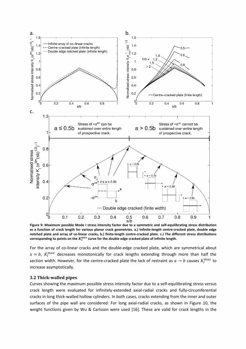
Curves of maximum stress intensity factor versus crack length are shown in Figure 9a and b. In the

interval 0 ≤ 𝑎 ≤𝑏

2, where a distribution of tensile stress saturated at 𝜎𝑙𝑖𝑚 can be sustained, 𝐾𝐼

𝑚𝑎𝑥 is

simply equal to the stress intensity factor for each crack under a uniform remote tensile load of

magnitude 𝜎𝑙𝑖𝑚. For the infinite array of co-linear cracks, for example, 𝐾𝐼𝑚𝑎𝑥 follows the first

expression in Equation 8. However, for cracks longer than 𝑏

2 the condition that the stress distribution

must self-equilibrate starts to have an effect on the 𝐾𝐼-maximising distribution of stress, and so

𝐾𝐼𝑚𝑎𝑥 decreases rapidly for longer cracks. It is important to note that the second half of each 𝐾𝐼

𝑚𝑎𝑥

curve shown in Figure 9 does not represent the stress intensity factor caused by any single

distribution of stress. Instead, for each crack length greater than 𝑏

2 there is a different self-

equilibrating stress distribution which maximises 𝐾𝐼. This is illustrated in Figure 9c.

a.

b.

c.

Figure 9: Maximum possible Mode I stress intensity factor due to a symmetric and self-equilibrating stress distribution as a function of crack length for various planar crack geometries. a.) Infinite-length centre-cracked plate, double edge notched plate and array of co-linear cracks, b.) finite-length centre-cracked plate. c.) The different stress distributions corresponding to points on the 𝑲𝑰

𝒎𝒂𝒙 curve for the double edge cracked plate of infinite length.

For the array of co-linear cracks and the double-edge cracked plate, which are symmetrical about

𝑥 = 𝑏, 𝐾𝐼𝑚𝑎𝑥 decreases monotonically for crack lengths extending through more than half the

section width. However, for the centre-cracked plate the lack of restraint as 𝑎 → 𝑏 causes 𝐾𝐼𝑚𝑎𝑥 to

increase asymptotically.

3.2 Thick-walled pipes

Curves showing the maximum possible stress intensity factor due to a self-equilibrating stress versus

crack length were evaluated for infinitely-extended axial-radial cracks and fully-circumferential

cracks in long thick-walled hollow cylinders. In both cases, cracks extending from the inner and outer

surfaces of the pipe wall are considered. For long axial-radial cracks, as shown in Figure 10, the

weight functions given by Wu & Carlsson were used [16]. These are valid for crack lengths in the

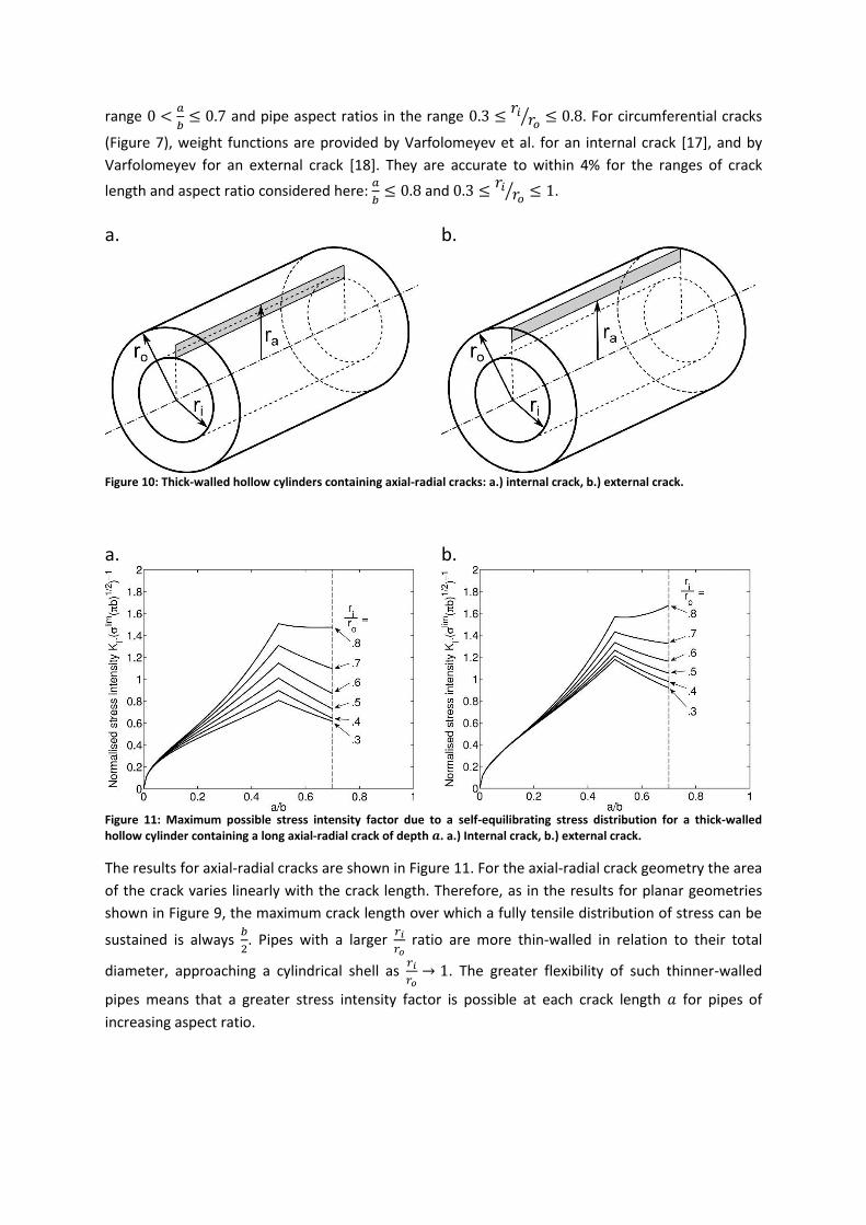
range 0 <𝑎

𝑏≤ 0.7 and pipe aspect ratios in the range 0.3 ≤

𝑟𝑖𝑟𝑜⁄ ≤ 0.8. For circumferential cracks

(Figure 7), weight functions are provided by Varfolomeyev et al. for an internal crack [17], and by

Varfolomeyev for an external crack [18]. They are accurate to within 4% for the ranges of crack

length and aspect ratio considered here: 𝑎

𝑏≤ 0.8 and 0.3 ≤

𝑟𝑖𝑟𝑜⁄ ≤ 1.

a.

b.

Figure 10: Thick-walled hollow cylinders containing axial-radial cracks: a.) internal crack, b.) external crack.

a.

b.

Figure 11: Maximum possible stress intensity factor due to a self-equilibrating stress distribution for a thick-walled hollow cylinder containing a long axial-radial crack of depth 𝒂. a.) Internal crack, b.) external crack.

The results for axial-radial cracks are shown in Figure 11. For the axial-radial crack geometry the area

of the crack varies linearly with the crack length. Therefore, as in the results for planar geometries

shown in Figure 9, the maximum crack length over which a fully tensile distribution of stress can be

sustained is always 𝑏

2. Pipes with a larger

𝑟𝑖

𝑟𝑜 ratio are more thin-walled in relation to their total

diameter, approaching a cylindrical shell as 𝑟𝑖

𝑟𝑜→ 1. The greater flexibility of such thinner-walled

pipes means that a greater stress intensity factor is possible at each crack length 𝑎 for pipes of

increasing aspect ratio.

a.

b.

Figure 12: Maximum possible stress intensity factor due to a self-equilibrating stress distribution for a thick-walled hollow cylinder containing a fully circumferential crack of depth 𝒂. a.) Internal crack, b.) external crack.

For the circumferential cracks illustrated in Figure 7, the maximum stress intensity factors are shown

in Figure 12. The area of a circumferential crack varies with the square of the crack length and

therefore the maximum crack length over which a tensile stress of magnitude 𝜎𝑙𝑖𝑚 can be sustained

is not constant for all 𝑟𝑖

𝑟𝑜, but is instead given by Equations 12 and 13. Consequently, the discontinuity

in each of the maximum 𝐾𝐼 curves shown in Figure 12 occurs at a different crack length.

4. Discussion

4.1 Assumptions, requirements and applicability

In our analysis, upper-bound values of stress intensity factor (𝐾𝐼𝑚𝑎𝑥) have been expressed in terms

of 𝜎𝑙𝑖𝑚, which is the maximum possible crack-normal component of the stress tensor (see Equation

3). To determine 𝐾𝐼𝑚𝑎𝑥 for a real structure it is necessary to first estimate 𝜎𝑙𝑖𝑚. One limitation of

the analysis presented is that it may be difficult to estimate 𝜎𝑙𝑖𝑚 accurately. This is a limitation

which is common to all methods for calculating stress intensity factor estimates without any explicit

characterisation of the residual stress field. Under purely uniaxial stress conditions in a perfectly

elastic-plastic material which exhibits no strain hardening, 𝜎𝑙𝑖𝑚 can be taken as the material’s

uniaxial elastic limit 𝜎𝑌. However, residual stress distributions containing a compressive hydrostatic

component can allow the crack-normal component of the stress tensor to exceed 𝜎𝑌. Likewise,

materials which exhibit significant strain hardening can contain residual stress states which would lie

outside of the yield surface of unhardened material. However, for residual stress fields in welded

metallic components it is generally reasonable to assume that the maximum tensile stress is

approximately the greater of the 0.2% proof stress of the parent and as-welded materials [3], [19].

For austenitic steels which work-harden strongly, R6 recommends using the 1% proof stress instead

[4]. Therefore, for the purposes of practical analysis it would normally be adequate to take 𝜎𝑙𝑖𝑚 as

some multiple of a measurable material proof strength, and this is done in Section 4.2.

In addition to the residual stress field being limited in magnitude, in this analysis it is also assumed

that the stress field is self-equilibrating; i.e. the crack-normal stress component integrates to zero

over the area of the section considered. Consequently, the maximum values of stress intensity factor

calculated are only valid for residual (or thermal) stress distributions which integrate to zero over

the section on which the defect exists. Some situations where this is the case are outlined in Section

2.1. This analysis is applicable to components which exhibit local or through-wall bending but not to

components subject to global bending, since the latter requires an externally-applied moment. For

the purpose of structural integrity assessment, the condition that the initial stress distribution must

be self-equilibrating only becomes important when the defect extends through the part of the stress

distribution which covers half the total section area. For shorter defects, 𝐾𝐼𝑚𝑎𝑥 is simply equal to the

stress intensity factor for a uniformly tensile crack-normal stress of magnitude 𝜎𝑙𝑖𝑚 across the

section. Therefore for short cracks this analysis offers no benefit in terms of reduced conservatism

over, for example, the use of assumed distributions of residual stress provided in the R6 and BS7910

procedures.

For this analysis it is assumed that on the plane of the defect, the crack-normal component of stress

varies in only one dimension. In some cases this is justifiable: for example, in autofrettaged tubes

and inertia friction welds the through-wall distribution of axial stress is normally independent of

circumferential position. However, in many cases this assumption is questionable. For example, it

would not be justified for a circumferential arc weld where weld start/stop features had a significant

effect on the residual stress field, or where or repair welding had been carried out at some point on

the circumference. In these cases, the assumption that the residual stress distribution must be self-

equilibrating over a single dimension is incorrect and 𝐾𝐼𝑚𝑎𝑥 calculated by the method described

above would not represent a rigorous upper bound. Therefore, to apply this method to welded

joints which may contain highly non-uniform residual stress fields, an analyst must first be confident,

through prior knowledge of the welding process, that the residual stress distribution on the plane of

the defect satisfies the conditions outlined in Section 2.1. A more general analysis, applicable to

residual stress fields which vary in more than one dimension on the defect plane, is described in

[11].

4.2 Comparison with 𝑲𝑰 from an assumed stress distribution

In this section, 𝐾𝐼𝑚𝑎𝑥 for a particular defect geometry is compared with stress intensity factors

calculated using assumed stress distributions given in the R6 weld residual stress distributions

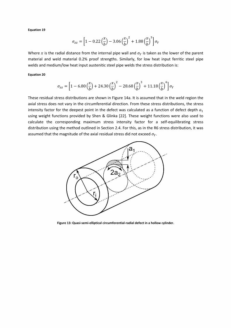
compendium [4], in order to illustrate the differences between these two approaches. A quasi-semi-

elliptical circumferential-radial defect on the inside of a pipe at a circumferential weld, with

geometry as described by Shiratori [20] and Bergman [21], is considered. This geometry is shown

schematically in Figure 13. The pipe radius ratio 𝑟𝑖

𝑟𝑜 is

10

11 and the aspect ratio

𝑎1

𝑎2 of the quasi-semi-

elliptical defect is 0.4. For circumferential welds in steel pipes, R6 Revision 4 gives through-thickness

distributions of axial residual stress categorised by weld heat input, which is calculated as [4]:

Equation 18

𝑄 =𝑞

𝑣𝑏

Where 𝑄 is the heat input per unit length per unit thickness, 𝑞 is the power of the welding torch

(uncorrected for arc efficiency), 𝑣 is the travel speed of the torch, and 𝑏 is the thickness of the

section being welded. Welds with 𝑄 > 120 𝐽 𝑚𝑚−2 are said to have high heat input, those with

50 < 𝑄 ≤ 120 𝐽 𝑚𝑚−2 have medium heat input, and those with 𝑄 ≤ 50 𝐽 𝑚𝑚−2 have low heat

input. For high heat input welds in ferritic and austenitic steel pipes the residual stress distribution is

given by:

Equation 19

𝜎𝑧𝑧 = [1 − 0.22 (𝑥

𝑏) − 3.06 (

𝑥

𝑏)2

+ 1.88 (𝑥

𝑏)3

] 𝜎𝑌

Where 𝑥 is the radial distance from the internal pipe wall and 𝜎𝑌 is taken as the lower of the parent

material and weld material 0.2% proof strengths. Similarly, for low heat input ferritic steel pipe

welds and medium/low heat input austenitic steel pipe welds the stress distribution is:

Equation 20

𝜎𝑧𝑧 = [1 − 6.80 (𝑥

𝑏) + 24.30 (

𝑥

𝑏)2

− 28.68 (𝑥

𝑏)3

+ 11.18 (𝑥

𝑏)4

] 𝜎𝑌

These residual stress distributions are shown in Figure 14a. It is assumed that in the weld region the

axial stress does not vary in the circumferential direction. From these stress distributions, the stress

intensity factor for the deepest point in the defect was calculated as a function of defect depth 𝑎1

using weight functions provided by Shen & Glinka [22]. These weight functions were also used to

calculate the corresponding maximum stress intensity factor for a self-equilibrating stress

distribution using the method outlined in Section 2.4. For this, as in the R6 stress distribution, it was

assumed that the magnitude of the axial residual stress did not exceed 𝜎𝑌.

Figure 13: Quasi-semi-elliptical circumferential-radial defect in a hollow cylinder.

a.

b.

Figure 14: Stress intensity factor results for the deepest point in a quasi-semi-elliptical circumferential-radial defect with

aspect ratio 𝒂𝟏

𝒂𝟐= 𝟎. 𝟒 embedded in a circumferential weld in a long hollow cylinder of aspect ratio

𝒓𝒊

𝒓𝒐=

𝟏𝟎

𝟏𝟏 . a.) Residual

stress distributions given in the R6 compendium. b.) Stress intensity factor as a function of crack depth for the R6 stress distributions, and the maximum possible stress intensity factor for a self-equilibrating state of stress.

In Figure 14b, the maximum possible stress intensity factor due to a self-equilibrating stress in this

geometry is plotted alongside the stress intensity factor due to the R6 weld residual stress

distributions. As noted previously, for shallow defects 𝐾𝐼𝑚𝑎𝑥 is simply equal to the stress intensity

factor for the same defect geometry subjected to a uniform yield-magnitude tensile stress. However,

𝐾𝐼𝑚𝑎𝑥 rapidly decreases for deeper cracks. Meanwhile, the stress distributions used in R6 are

deliberately non-self-equilibrating, and as a consequence the calculated 𝐾𝐼 for a low heat input weld

exceeds 𝐾𝐼𝑚𝑎𝑥 at crack depths greater than 𝑎1 = 0.64𝑏.

The fundamental difference between the approach typically used to analyse the residual stress

contribution to 𝐾𝐼 and the one proposed here concerns the assumptions which are made about the

form of the residual stress field. In structural integrity assessment procedures such as R6 and

BS7910, any unknown distribution of residual stress is assumed to be described by a specific function

(Equation 19 or Equation 20, for example). The necessary stress function is obtained from a

compendium of functions which are deliberately conservative. By contrast, to find 𝐾𝐼𝑚𝑎𝑥 no

particular form of the residual stress distribution is assumed, but it is taken that the stress field is

self-equilibrating across the section being analysed. This has the advantage that the analyst needs

less information about the object to calculate an upper bound value for 𝐾𝐼. For instance, in the

example of a welded pipe they would not need to know the heat input used to make the weld; 𝐾𝐼𝑚𝑎𝑥

depends only on the object’s geometry and the maximum crack-normal stress that can be sustained

by the material.

4.3 Comparison with an eigenstrain–based method of estimating 𝑲𝑰𝒎𝒂𝒙

A general method for approximating the maximum contribution of residual stress to 𝐾𝐼, based on

inverse eigenstrain analysis [23], has been described previously by the authors [11]. In this method,

the residual stress fields and stress intensity factors which arise from a number of basis distributions

of incompatible inelastic strain (eigenstrain) are determined. Then, the weighted sum of these which

maximises the stress intensity factor is found. This maximisation must be subject to a constraint

which represents the material’s finite capacity to support stress, for example that the von Mises

stress may not exceed the material’s yield stress anywhere in the body. This provides an

approximation for 𝐾𝐼𝑚𝑎𝑥 given the assumption that the set of eigenstrain basis distributions used

can, as a weighted sum, closely approximate any possible distribution on eigenstrain in the object.

Results from this method can be compared with those from the present weight function–based

analysis.

For a long thick-walled hollow cylinder with aspect ratio 𝑟𝑖

𝑟𝑜= 0.8 containing a fully circumferential

internal crack (as in Figure 7a), an approximation of 𝐾𝐼𝑚𝑎𝑥(𝑎) was obtained using the eigenstrain-

based approach. The cylinder wall was assumed to contain distributions of eigenstrain (and hence

residual stress) which only varied through the wall thickness. A set of eigenstrain basis functions was

generated to allow the eigenstrain distribution to be approximated using three 15th-order Fourier

series; one to represent each finite component of the eigenstrain tensor. The whole basis set is

made up of the sub-sets for each eigenstrain component:

Equation 21

𝜀𝑖𝑗𝑘∗ (𝑥) = 𝜀11𝑛

∗ (𝑥) ∪ 𝜀22𝑛∗ (𝑥) ∪ 𝜀33𝑛

∗ (𝑥)

where 𝜀𝑖𝑗𝑘∗ (𝑥) is a set of 𝑘 eigenstrain distributions 𝜀𝑖𝑗

∗ (𝑥), and:

Equation 22

𝜀11𝑛∗ (𝑥) = (

𝑓𝑛(𝑥) 0 00 0 00 0 0

)

𝜀22𝑛∗ (𝑥) = (

0 0 00 𝑓𝑛(𝑥) 00 0 0

)

𝜀33𝑛∗ (𝑥) = (

0 0 00 0 00 0 𝑓𝑛(𝑥)

)

where 𝑓𝑛(𝑥) represents the set of Fourier series terms given by:

Equation 23

𝑓𝑛(𝑥) = 𝑒𝑖2𝜋𝑛𝑥𝑏

𝑓𝑜𝑟 𝑛 = 0, 1,2…15

Here 𝜀𝑖𝑗𝑘∗ (𝑥) contains 93 unique basis functions: (15 x 2) + 1 = 31 for each of the three eigenstrain

tensor components. For each of the basis functions in this set, the residual stress distribution in an

uncracked pipe and the corresponding Mode I stress intensity factor was determined from finite

element analysis performed using the Abaqus/Standard v6.12 solver [24]. Using a combination of

these basis function solutions, the stress intensity factor for each crack length was maximised

subject to the condition that the maximum crack-normal stress could not exceed 𝜎𝑙𝑖𝑚. The process

of estimating 𝐾𝐼𝑚𝑎𝑥 using constrained maximisation is described elsewhere [11].

a.

b.

Figure 15: a.) Comparison of solutions for the maximum possible Mode I stress intensity factor due to a self-equilibrating stress distribution for a long thick-walled hollow cylinder containing a fully circumferential internal crack. The weight function method is exact to the accuracy of the underlying weight function solution. b.) 𝑲𝑰-maximising stress

distributions generated by each method for a crack length of 𝒂

𝒃= 𝟎. 𝟕𝟓.

A comparison of 𝐾𝐼𝑚𝑎𝑥 for this geometry as predicted by the two methods is shown in Figure 15a.

The accuracy of the weight-function-based method is dependent on the accuracy of the underlying

weight function solution (believed to be better than 4% in this case [17]). However, the accuracy of

the eigenstrain-based approximation is limited by the fact that the eigenstrain distribution must be

represented by the basis set used. As shown in Figure 15b, the sharp stress reversals seen in the

stress distribution determined using the weight function method cannot be replicated using the

Fourier basis of the eigenstrain-based solution. This is particularly true for cracks longer than 𝑎𝑡

(where 𝑎𝑡 = 0.528𝑏 in this example), because for these cracks the true 𝐾𝐼-maximising through-wall

stress distribution as determined by weight function method is more complex. Since the true 𝐾𝐼-

maximising stress field cannot be represented exactly using this limited basis set, the eigenstrain-

based method gives values of 𝐾𝐼𝑚𝑎𝑥 for deeper cracks which are slightly lower than the true upper

bound.

4.4 𝑲𝑰𝒎𝒂𝒙 and corresponding 𝑲𝑰-maximising stress distributions

The 𝐾𝐼-maximising stress field for a given geometry and crack length (as shown in Figure 6d and

Figure 15b for example) may be complex and may contain several points at which tensile and

compressive stresses of yield magnitude exist directly adjacent to one another. These stress reversal

points must also occur at particular locations on the section. In most circumstances a sectional

residual stress distribution of this sort would be unrealistic, because there are few processes capable

of introducing the exact pattern of plastic deformation necessary to produce such a stress

distribution. 𝐾𝐼𝑚𝑎𝑥 therefore represents only a theoretical maximum, and the Mode I stress intensity

factor associated with any (one-dimensional) residual stress distribution likely to be encountered in

a real component would necessarily be lower than this value. Consequently, 𝐾𝐼𝑚𝑎𝑥 could be used as

a basic check on any analytical or experimental evaluation of 𝐾𝐼 for a particular crack

geometry/residual stress combination: a value of 𝐾𝐼 greater than 𝐾𝐼𝑚𝑎𝑥 for the same geometry

would indicate an error.

5. Conclusions A procedure for calculating the maximum possible Mode I stress intensity factor for a planar crack in

a self-equilibrating stress field has been presented. This can be used to provide an upper bound

value of 𝐾𝐼 for a given defect subject to an unknown one-dimensional distribution of residual stress

or thermal stress. A prerequisite for the analysis is that point-force weight functions are available for

the defect geometry being analysed. Using this method, normalised values of the maximum Mode I

stress intensity factor have been determined for a number of common crack geometries, including

infinitely-extended axial-radial cracks and fully-circumferential cracks in long thick-walled pipes with

a range of wall thickness ratios and crack depths.

For a given crack, the maximum possible Mode I stress intensity factor which can be applied by a

self-equilibrating stress deviates from the Mode I stress intensity factor for an applied tensile stress

of yield magnitude only when a crack extends a significant distance through the section. This is

because at shorter crack lengths it is possible for tensile residual stress to be sustained across the

whole (prospective) crack area. However, for deeper cracks the method provides a useful upper

bound to the stress intensity factor which could be present due to internal stressing, and does not

require any knowledge of the actual stress distribution which exists in the object being analysed.

Acknowledgements This work was supported by a Rolls-Royce/EDF Energy/Royal Academy of Engineering chair awarded

to DJS.

Supplementary material The weight function based methods for determining 𝐾𝐼

𝑚𝑎𝑥 described in this article were

implemented in MATLAB [25] code. A package of analysis scripts, which includes the weight

functions for a small library of example defect geometries (including all of the cases discussed in this

article) is available for download via the following link: [insert link here].

References [1] P. J. Withers, “Residual stress and its role in failure,” Reports on Progress in Physics, vol. 70,

no. 12, pp. 2211–2264, 2007. [2] U. Zerbst, R. A. Ainsworth, H. Beier, H. Pisarski, Z. L. Zhang, K. Nikbin, T. Nitschke-Pagel, S.

Münstermann, P. Kucharczyk, and D. Klingbeil, “Review on fracture and crack propagation in weldments - A fracture mechanics perspective,” Engineering Fracture Mechanics, vol. 132, pp. 200–276, 2014.

[3] BSi, BS 7910 - Guide to methods for assessing the acceptability of flaws in metallic structures. BSi, 2013.

[4] “R6: Assessment of the Integrity of Structures Containing Defects, Revision 4, Amendment 10,” EDF Energy, Gloucester, 2013.

[5] P. J. Budden and J. K. Sharples, “Treatment of secondary stresses,” in Comprehensive Structural Integrity, Volume 7, 1st ed., R. A. Ainsworth and K.-H. Schwalbe, Eds. Elsevier-Pergamon, 2003, pp. 245–288.

[6] P. Dong, “Length scale of secondary stresses in fracture and fatigue,” International Journal of Pressure Vessels and Piping, vol. 85, no. 3, pp. 128–143, 2008.

[7] D. P. G. Lidbury, “The significance of residual stresses in relation to the integrity of LWR pressure vessels,” International Journal of Pressure Vessels and Piping, vol. 17, no. 4, pp. 197–328, 1984.

[8] P. J. Bouchard, P. J. Budden, and P. J. Withers, “Fourier basis for the engineering assessment of cracks in residual stress fields,” Engineering Fracture Mechanics, vol. 91, pp. 37–50, 2012.

[9] D. Green and J. Knowles, “The treatment of residual stress in fracture assessment of pressure vessels,” Journal of Pressure Vessel Technology, Transactions of the ASME, vol. 116, no. 4, pp. 345–352, 1994.

[10] E. Smith, “Fracture assessment of pressure vessels: the treatment of weld residual stresses and thermal stresses,” in PVP Vol. 280: Fatigue, Flaw Evaluation and Leak-Before-Break Assessments, 1994, vol. 280, pp. 109–117.

[11] H. E. Coules and D. J. Smith, “Approximating the upper bound in elastic stress intensity factor for a crack in an unknown residual stress field,” Engineering Fracture Mechanics, vol. 136, pp. 226–240, 2015.

[12] H. F. Bueckner, “Field singularities and related integral representations,” in Methods of Analysis and Solutions of Crack Problems, vol. 1, G. C. Sih, Ed. Noordhoff International, 1973, pp. 239–314.

[13] J. R. Rice, “Some remarks on elastic crack-tip stress fields,” International Journal of Solids and Structures, vol. 8, no. 6, pp. 751–758, 1972.

[14] H. Tada, P. C. Paris, and G. R. Irwin, The Stress Analysis of Cracks Handbook, 3rd ed. Professional Engineering Publishing, 2000.

[15] G. R. Irwin, “Analysis of stresses and strains near the end of a crack traversing a plate,” Journal of Applied Mechanics, Transactions of the ASME, vol. 24, no. 24, pp. 361–364, 1957.

[16] X. R. Wu and A. J. Carlsson, Weight Functions and Stress Intensity Factor Solutions. Pergamon Press, 1991.

[17] I. V. Varfolomeyev, M. Petersilge, and M. Busch, “Stress intensity factors for internal circumferential cracks in thin- and thick-walled cylinders,” Engineering Fracture Mechanics, vol. 60, no. 5–6, pp. 491–500, 1998.

[18] I. V. Varfolomeyev, “Weight function for external circumferential cracks in hollow cylinders subjected to axisymmetric opening mode loading,” Engineering Fracture Mechanics, vol. 60, no. 3, pp. 333–339, 1998.

[19] R. H. Leggatt, “Residual stresses in welded structures,” International Journal of Pressure Vessels and Piping, vol. 85, no. 3, pp. 144–151, 2008.

[20] M. Shiratori, “Analysis of stress intensity factors for surface cracks in pipes by an influence function method,” in Advances in Fracture and Fatigue for the 1990’s: Proceedings of the 1989 Pressure Vessels and Piping Conference, 1989, vol. 167, pp. 45–50.

[21] M. Bergman, “Stress intensity factors for circumferential surface cracks in pipes,” Fatigue and Fracture of Engineering Materials and Structures, vol. 18, no. 10, pp. 1155–1172, 1995.

[22] G. Shen and G. Glinka, “Stress intensity factors for internal edge and semi-elliptical cracks in hollow cylinders,” in High Pressure - Codes, Analysis and Applications: Proceedings of the 1993 Pressure Vessels and Piping Conference, 1993, vol. 263, pp. 73–79.

[23] T.-S. Jun and A. M. Korsunsky, “Evaluation of residual stresses and strains using the eigenstrain reconstruction method,” International Journal of Solids and Structures, vol. 47, no. 13, pp. 1678–1686, 2010.

[24] Abaqus/Standard, v6.12. Providence, RI, USA: Dassault Systemes Simulia Corp. [25] MATLAB®, version 8.1.0.604 (R2013a). Natick, USA: The Mathworks Inc.