copula-based models for risk analysis of process …
TRANSCRIPT
COPULA-BASED MODELS FOR RISK ANALYSIS OF PROCESS SYSTEMS
WITH DEPENDENCIES
by
© Chuanqi Guo
A Thesis submitted to the
School of Graduate Studies
in partial fulfilment of the requirements for the degree of
Master of Engineering
Faculty of Engineering and Applied Science
Memorial University of Newfoundland
May 2019
St. John’s Newfoundland
i
Abstract
With the increasing integration of heat and mass and the complexity of process systems,
process variables are becoming strongly interdependent. Ignoring these dependencies in
process safety modelling is unreasonable. The present work addresses this dependency
challenge. It proposes two simple yet robust risk models for process safety analysis.
The first model is the copula-based bow-tie (CBBT) model, which revises the traditional bow-
tie (BT) model by considering dependencies among the causes and failures of safety barriers.
Copulas are used to simulate hypothetical dependent joint probability densities. The proposed
model, along with classical BT analysis, is examined under a case study of the risk analysis of
a typical distillation column. Comparing the results from both approaches in terms of the
estimated probability of a potential hexane release scenario, it is shown that the dependencies
of process units’ malfunctions can increase the likelihood of accident scenarios to a significant
extent. Further, to explore the mechanisms behind the impact of such dependencies, the effect
of dependencies on the two most basic logic gates is also analyzed.
The next model developed is the copula-based Bayesian network (CBBN), which integrates
linear dependence modelled by a Bayesian network (BN) and non-linear dependence by
copulas. It provides more reliable estimation of accident probability when applied to real cases.
Sensitivity analysis identifies the factors that play important roles in causing an accident. A
diagnostic analysis is also performed to find the most probable explanation for the occurred
event. Results match the accident investigation report and thus prove the effectiveness of the
proposed model.
Key words: Risk assessment; Bow-tie; Bayesian network; Dependence; Copula; Process safety;
Accident model
ii
Acknowledgements
At first, I would like to thank my supervisor Dr. Faisal Khan and co-supervisor Dr. Syed Imtiaz
for their valuable help throughout the program of my graduate study. Dr. Khan is an
enthusiastic scholar and supervisor, who always encourages me to conduct challenging
research work for the purpose of realizing my full potential. The work environment under his
supervision is so free and flexible that I can arrange where and when to study as I like. This
stimulates me to become a self-learner. However, he is always there willing to help whenever
I meet problems or get confused in research. Dr. Khan is strict with work quality and gives me
guidance and suggestions in perfecting the work, all of which have contributed to training me
to be a qualified researcher.
Dr. Imtiaz is kind and have come up with many helpful tips about the proper organization of
research papers and scientific writing. I have harvested publications and more importantly
confidence thanks to their help.
This research work has been made possible from the financial support provided by the Natural
Science and Engineering Research Council of Canada (NSERC) through the Discovery Grant
program and the Canada Research Chair (Tier I) program in offshore safety and risk
Engineering.
I am also grateful to the fellows of Centre for Risk, Integrity and Safety Engineering (C-RISE)
who have motivated me in course study and research stages. Finally, I would like to send my
thanks to my parents, my friends here and back home for their care, encouragement and
company in the two unforgettable years.
iii
Table of Contents Abstract ......................................................................................................................................... i
Acknowledgements ...................................................................................................................... ii
Table of Contents ........................................................................................................................ iii
List of Tables ............................................................................................................................... vi
List of Figures ........................................................................................................................... viii
List of Abbreviations ................................................................................................................... ix
Co-authorship Statement .............................................................................................................. x
Chapter 1. Introduction and Overview................................................................. 1
Quantitative Risk Analysis ............................................................................................... 1
Specific QRA approaches ................................................................................................. 5
Dependency in risk assessment of process systems .......................................................... 6
Research scope and objective ........................................................................................... 8
Novelty and contributions ................................................................................................. 9
Thesis structure ............................................................................................................... 10
References ...................................................................................................................... 11
Chapter 2. Risk assessment of process system considering dependencies ....... 16
Introduction .................................................................................................................... 17
The proposed risk assessment methodology ................................................................... 19
Step 1: Identify accident scenario ........................................................................... 20
Step 2: Develop bow-tie model ............................................................................... 21
Step 3: Derive occurrence probabilities of IEs and failure probabilities of SBs ..... 23
Comparison study: Estimate TE and OEs probabilities considering independence of
IEs and SBs ............................................................................................................................ 24
Step 4: Estimate TE and OEs probabilities considering interdependence of IEs and
SBs 25
Step 5: Estimate the probability of major OEs ........................................................ 32
Application of the proposed methodology...................................................................... 33
Steps 1-2: Identify accident scenarios and then develop the bow-tie model ........... 35
Step 3: Derive occurrence probabilities of IEs and failure probabilities of SBs ..... 36
Comparison study: Estimate TE and OEs probabilities considering independence of
IEs, CEs and SFs .................................................................................................................... 38
iv
Step 4: Estimate TE and OEs probabilities considering interdependence of IEs, CEs
and SFs 39
Step 5: Estimate the probability of major outcome events ...................................... 42
Discussion ....................................................................................................................... 42
The effect of interdependence on the probability of the top event .......................... 42
The effect of interdependence on the probability of the outcome events ............... 43
Conclusions .................................................................................................................... 44
References ...................................................................................................................... 45
Chapter 3. Copula-based Bayesian network model for process system risk
assessment 48
Introduction .................................................................................................................... 49
The proposed copula-based Bayesian network model .................................................... 51
3.2.1 Step 1: Identify network nodes ............................................................................... 52
3.2.2 Step 2: Develop Bayesian network ......................................................................... 53
3.2.3 Step 3: Assign occurrence probabilities to network nodes ..................................... 54
3.2.4 Step 4: Add copula functions to the developed Bayesian network ......................... 55
3.2.5 Step 5: Estimate the outcome event probabilities of the developed CBBN ............ 56
3.2.6 Comparison: Estimate the outcome event probabilities of the developed BN ........ 59
3.2.7 Discussion of the results for the example ............................................................... 59
Application of the copula-based Bayesian network ....................................................... 60
3.3.1 Steps 1-2: Identify network nodes and develop Bayesian network......................... 61
3.3.2 Step 3: Determine occurrence probabilities of network nodes ............................... 64
3.3.3 Step 4: Integrate copula functions to the developed Bayesian network .................. 67
3.3.4 Step 5: Estimate the top event and outcome event probabilities of the developed
CBBN 69
3.3.5 Comparison: Estimate the top event and outcome event probabilities of the
developed BN......................................................................................................................... 70
Discussion ....................................................................................................................... 70
3.4.1 The top event probability in CBBN and BN ............................................................... 70
3.4.2 The outcome event probabilities in CBBN and BN .................................................... 71
Sensitivity analysis ......................................................................................................... 72
Probability updating........................................................................................................ 75
Conclusions .................................................................................................................... 77
References ...................................................................................................................... 78
v
Chapter 4. Summary ............................................................................................ 82
4.1 Conclusions .................................................................................................................... 82
4.1.1 Development of copula-based bow-tie model ......................................................... 83
4.1.2 Development of copula-based Bayesian network model ........................................ 84
4.2 Future work ..................................................................................................................... 84
vi
List of Tables
Table 2.1 Probability distributions for the IEs. ................................................................. 24
Table 2.2 Probability distributions for the SBs. ................................................................ 24
Table 2.3 One of the correlation matrices for the case A∩B∩C. ...................................... 27
Table 2.4 Occurrence probabilities of the TE and the OEs in the case study. .................. 32
Table 2.5 Safety and protection systems. .......................................................................... 35
Table 2.6 The probabilities of the CEs and the failure probabilities of the SFs. .............. 37
Table 2.7 Components of the IEs and their probabilities. ................................................. 37
Table 2.8 Correlation parameters among IEs. ................................................................... 40
Table 2.9 Correlation parameters among CEs and SFs. .................................................... 40
Table 2.10 Result summary of occurrence probabilities of FOP, the TE and OEs. .......... 41
Table 3.1 Possible outcome events based on the state combination of nodes A, B and C.53
Table 3.2 Occurrence probabilities of the network nodes in the example. ....................... 55
Table 3.3 Correlation parameters for the example. ........................................................... 56
Table 3.4 Occurrence probabilities of the OEs for the example in BN and CBBN. ......... 57
Table 3.5 Outcome event nodes depending on the performance of safety nodes. ............ 63
Table 3.6 Occurrence probabilities of the cause nodes. .................................................... 64
Table 3.7 Safety nodes and their probabilities (CCPS (2001); OREDA (2002)). ............. 66
Table 3.8 Correlation parameters between the causes of quench water entering Reboiler B.
........................................................................................................................................... 67
Table 3.9. Correlation parameters within quench water flow control system. ................. 68
Table 3.10 Correlation parameters between the causes of Reboiler B isolated from
vii
overpressure protection. .................................................................................................... 68
Table 3.11 Correlation parameters among safety nodes. .................................................. 68
Table 3.12 Result summary of occurrence probabilities of the top event and outcome events
in both BN and CBBN. ..................................................................................................... 69
Table 3.13 Updated probabilities of the nodes for OE6. ................................................... 76
viii
List of Figures
Figure 1.1 QRA steps adapted from Hashemi (2016). ........................................................ 3
Figure 2.1 Methodology for risk assessment considering dependence. ............................ 20
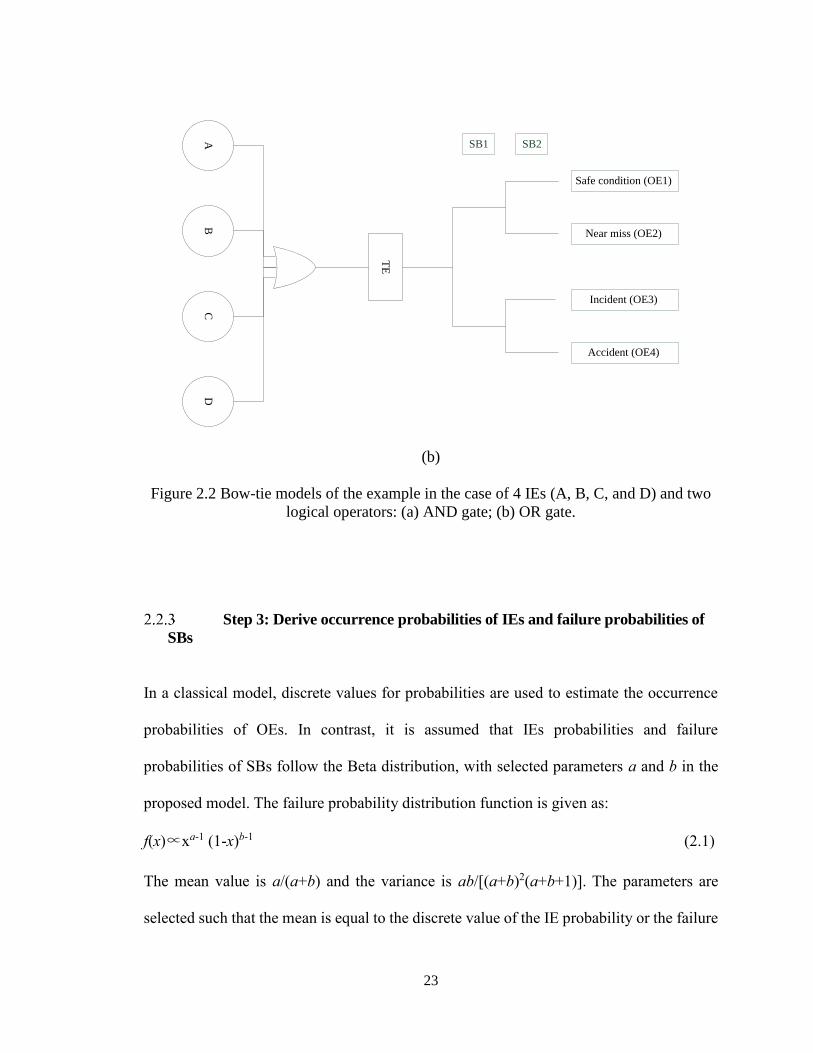
Figure 2.2 Bow-tie models of the example in the case of 4 IEs (A, B, C, and D) and two
logical operators: (a) AND gate; (b) OR gate. .................................................................. 23
Figure 2.3 The effect of interdependence among IEs on the probability of TE for AND gate
example; data is also presented for analysis. .................................................................... 29
Figure 2.4 The effect of interdependence among IEs on the probability of TE for OR gate
example; data is also presented for analysis. .................................................................... 31
Figure 2.5 Hexane distillation column adapted from Markowski and Kotynia (2011). ... 34
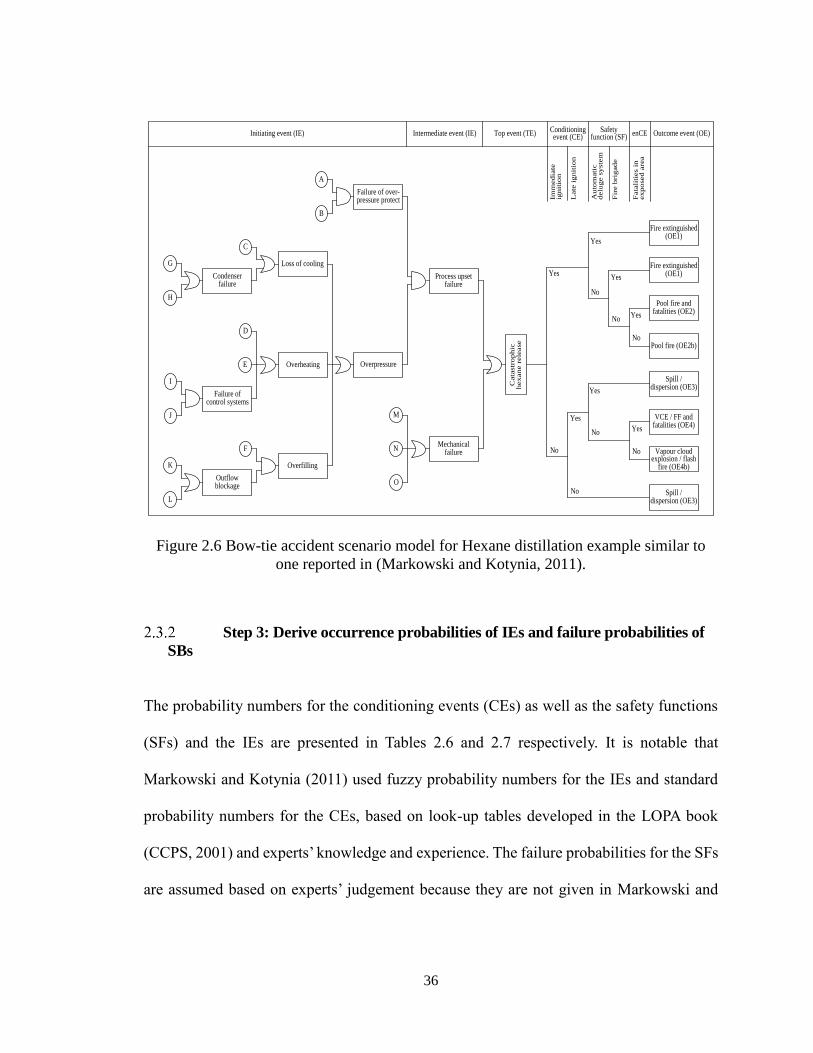
Figure 2.6 Bow-tie accident scenario model for Hexane distillation example similar to one
reported in (Markowski and Kotynia, 2011). .................................................................... 36
Figure 3.1 Steps for developing a CBBN. ........................................................................ 52
Figure 3.2 BN model for the example. ............................................................................. 54
Figure 3.3 Variation of OE2 probability as dependence strength changes. (Data also
included) ........................................................................................................................... 58
Figure 3.4 Propylene fractionator column (CSB,2016). ................................................... 61
Figure 3.5 Bayesian network for propane release from Reboiler B. ................................ 63
Figure 3.6 Sensitivity analysis for OE6 in BN. ................................................................ 73
Figure 3.7 Sensitivity analysis for OE6 in CBBN. ........................................................... 73
Figure 3.8 Diagnostic analysis of OE6. ............................................................................ 76
ix
List of Abbreviations
BN Bayesian network
BPCS Basic process control systems
BT Bow-tie
CBBN Copula-based Bayesian network
CBBT Copula-based Bow-tie
CE Conditioning event
CPT Conditional probability tables
ET Event tree
ETA Event tree analysis
FMEA Failure mode and effect analysis
FT Fault tree
FTA Fault tree analysis
HAZOP Hazard and operability study
IE Initiating event
MCS Minimum cut set
OE Outcome event
QRA Quantitative risk analysis
SB Safety barrier
SIF Safety instrumented functions
SIS Safety instrumented systems
SF Safety function
TE Top event

x
Co-authorship Statement
For all the work presented in this thesis, I am the principal author. In the design stage, my
supervisor identified the research gap to be filled, which helped me to write the research
proposal. I reviewed the literature and developed two revised methodologies to overcome the
limitations of the currently widely used risk analysis methodologies. I applied these
methodologies to practical studies, obtained simulation data and then analyzed the results. In
this procedure, Dr. Faisal Khan helped by offering suggestions towards the selection of specific
research aspects, such as recommending me to perform sensitivity analysis and probability
updating. He contributed to reviewing and approving the discussions of results as well. I
prepared the draft of the manuscript and revised it based on the feedback from Drs. Faisal Khan
and Syed Imtiaz.
1
Chapter 1. Introduction and Overview
Complex process operations involving large inventories of hazardous materials have
serious safety concerns. The loss of material in such facilities may lead to low-probability
but high-consequence events (Pasman, 2015), such as significant economic loss,
environmental damage or multiple fatalities or injuries. These concerns are quantified in
terms of financial and personnel risk. Past major accidents, for example, Bhopal (1984),
Piper Alpha (1988) and Buncefield (2005), have led to the establishment of process safety
management regulations. While process safety management is effective, its full potential
has not yet been reached. Also, as the complexity of operations is on the rise, accident
causation is becoming more complex and harder to estimate and predict (Vaughen and
Kletz, 2012). This situation underscores the need for better estimation of these accident
scenarios, their likelihood, quantitative risk and subsequently better safety management
practices, and many qualitative and quantitative analysis methods have been developed to
meet this need.
Quantitative Risk Analysis
In the past, qualitative analysis was widely used for the risk assessment of hazardous
substances. However, one of its obvious drawbacks is its vagueness in terminology, such
as the description “a high degree of protection” (Buncefield Major Investigation Board,
2008). On the other hand, Quantitative Risk Analysis (QRA) is easy to perform and is now
widely applied because the computational burden has been lessened thanks to technological
progress.
2
QRA was first used in nuclear plants. In the 1970s, the probabilistic risk assessment for the
nuclear sector was developed by the United States Nuclear Regulatory Commission. It was
only at a later stage that QRA was applied to chemical process safety management. In 2012,
Seveso, the European industrial safety regulatory agency, issued its third generation of
safety regulations (Seveso III directive) (EU, 2012), which apply to more than 10,000
industrial establishments, many of which are chemical plants (European Commission -
Environment Directorate, 2015). As a widely-used approach, QRA has been adopted to
facilitate the implementation of Seveso regulations (Pasman and Reniers, 2014).
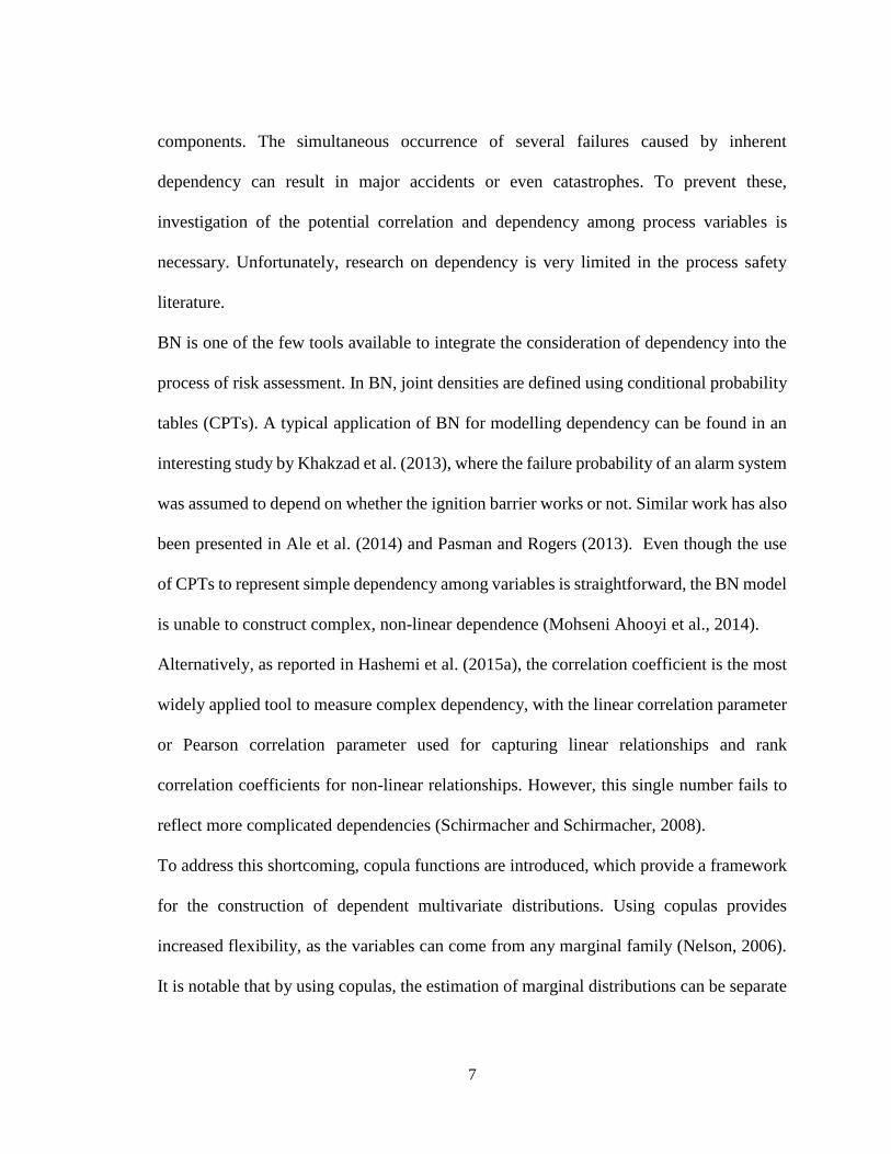
The latest trend in the development in QRA has been towards dynamic risk analysis (Villa
et al., 2016). Dynamic QRA makes use of newly available information on the process
system such as accident precursors or alarm databases to continuously update the risk level.
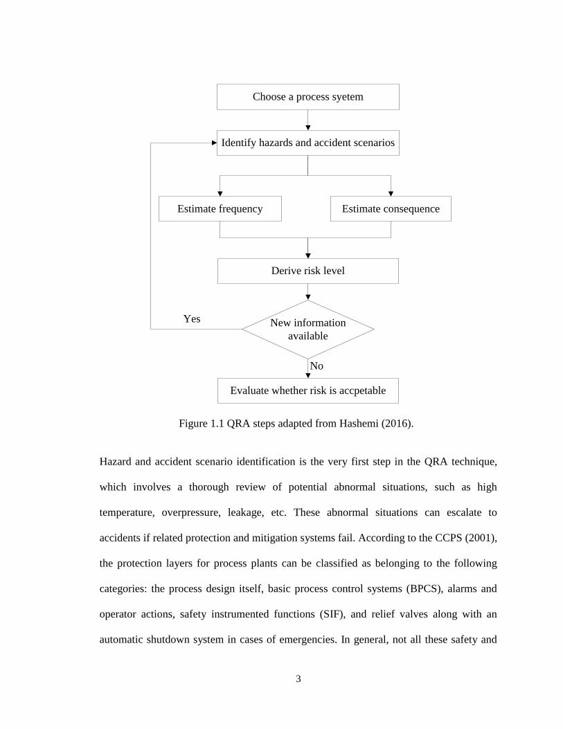
The steps involved in dynamic QRA are shown in Fig. 1.1. From this comprehensive
perspective, dynamic QRA is considered a robust tool for hazard and risk quantification of
a process facility.
3
Identify hazards and accident scenarios
Derive risk level
Estimate frequency Estimate consequence
Choose a process syetem
Evaluate whether risk is accpetable
New information
available
Yes
No
Figure 1.1 QRA steps adapted from Hashemi (2016).
Hazard and accident scenario identification is the very first step in the QRA technique,
which involves a thorough review of potential abnormal situations, such as high
temperature, overpressure, leakage, etc. These abnormal situations can escalate to
accidents if related protection and mitigation systems fail. According to the CCPS (2001),
the protection layers for process plants can be classified as belonging to the following
categories: the process design itself, basic process control systems (BPCS), alarms and
operator actions, safety instrumented functions (SIF), and relief valves along with an
automatic shutdown system in cases of emergencies. In general, not all these safety and
4
control systems are applied. The number of incorporated safety systems depends on the
risk acceptance criteria required by the regulating authorities.
As is reported by CCPS (2003), there are many methods available for the hazard
identification of a process system: Hazard and Operability Study (HAZOP), Failure Mode
and Effect Analysis (FMEA), safety checklists, etc. To limit the focus to severe hazards or
credible scenarios, one may employ the maximum credible accident scenario analysis
approach proposed by Khan and Abbasi (2002).
The next risk analysis steps refer to the estimation of frequencies of identified accidents
and their potential consequences. This estimation can be carried out by means of
probabilistic and engineering models (Crowl and Louvar, 2011).
Frequency estimation calls for the collection of failure rates or probabilities of failure in
demand data. Such generic data are usually based on expert judgement and process
empirical knowledge and can be collected from databases such as OREDA (2002), TNO
(2005a), HSE (2009), etc. If available, plant-specific data from historical records is the best
source to be integrated into the calculations. Even though such probabilistic estimation
cannot fully reflect reality, it still offers meaningful and detailed predictions of potential
risks.
Consequence estimation involves the determination of possible effects in terms of health
loss, property loss and environmental damage resulting from undesired scenarios. There
are many mathematical and empirical models available for the estimation of consequences.
Interested readers may refer to Crowl and Louvar (2011) and Assael and Kakosimos (2010)
for an exhaustive description of source models, fires, explosions and toxic gas dispersion
5
calculations. In addition, Yang et al. (2018) used computational fluid dynamics to simulate
fire in a floating liquefied natural gas facility. As an alternative, Hashemi et al. (2014)
developed loss functions for the overall consequence assessment of process deviations
modelling five major loss categories: quality, production, asset, human health and
environmental losses.
The risk level is established once the estimation results of frequency and consequence are
determined. If new information on the behavior of the process system becomes available,
new hazards may be identified, and the present risk level should be revised by estimating
the frequency and consequence again. This updated risk profile is then compared with the
acceptability criteria to confirm if it meets the requirements.
Specific QRA approaches
While the previous section contributes to the overview of QRA, the current section
introduces the most common approaches to performing QRA, especially for hazard
identification and frequency estimation procedures.
Fault tree analysis (FTA) is a typical graphical QRA tool. When performing FTA, the top
event, usually the release of hazardous materials from a container, is identified first. Next,
all the possible intermediate and basic events such as the occurrence of abnormal
conditions and the subsequently unfortunate failures of protection systems are found by
conducting a causal analysis. The top event probability can then be obtained from the
logistics shown in the developed fault tree.
Similar to FTA, event tree analysis (ETA) is also an easily-adopted risk assessment method.
6
ETA consists of many branches, which start from an unwanted event, normally known as
the top event, and end with different outcomes. The outcomes will differ based on the
performance of safety barriers that are supposed to reduce the effects of the top event.
Combining FTA and ETA will lead to the bow-tie (BT) diagram, which is considered a
comprehensive QRA technique, since it presents both the causes and the consequences of
a top event. Some recent adoptions of BT in chemical process safety analysis can be found
in Aqlan and Mustafa Ali (2014) and Lu et al. (2015).
Among the most recently used QRA techniques is Bayesian network (BN). BN is defined
as a directed acyclic graph based on Bayes’ theorem (Mittnik and Starobinskaya, 2010).
One of the features of BN is its capabilities in updating prior beliefs when new information
becomes available. In the field of chemical process application, the accident precursor data
collected throughout the lifecycle of a plant can be used to dynamically adapt the failure
probabilities of the safety barriers. Based on this, a real-time risk monitoring platform is
built, which is very useful in supervising the fast-changing operation conditions of a plant.
Dependency in risk assessment of process systems
When conducting traditional process safety and risk analysis, it is often assumed that there
is no dependency in the causations. Nevertheless, such an assumption is no longer
convincing due to process integration. Taking a complex chemical plant as an example, the
components within the same system, e.g., a temperature safety instrumented system, or
across systems work under similar circumstances and thus are subject to similar
temperature, pressure and stress. This leads to correlated failure probabilities of these
7
components. The simultaneous occurrence of several failures caused by inherent
dependency can result in major accidents or even catastrophes. To prevent these,
investigation of the potential correlation and dependency among process variables is
necessary. Unfortunately, research on dependency is very limited in the process safety
literature.
BN is one of the few tools available to integrate the consideration of dependency into the
process of risk assessment. In BN, joint densities are defined using conditional probability
tables (CPTs). A typical application of BN for modelling dependency can be found in an
interesting study by Khakzad et al. (2013), where the failure probability of an alarm system
was assumed to depend on whether the ignition barrier works or not. Similar work has also
been presented in Ale et al. (2014) and Pasman and Rogers (2013). Even though the use
of CPTs to represent simple dependency among variables is straightforward, the BN model
is unable to construct complex, non-linear dependence (Mohseni Ahooyi et al., 2014).
Alternatively, as reported in Hashemi et al. (2015a), the correlation coefficient is the most
widely applied tool to measure complex dependency, with the linear correlation parameter
or Pearson correlation parameter used for capturing linear relationships and rank
correlation coefficients for non-linear relationships. However, this single number fails to
reflect more complicated dependencies (Schirmacher and Schirmacher, 2008).
To address this shortcoming, copula functions are introduced, which provide a framework
for the construction of dependent multivariate distributions. Using copulas provides
increased flexibility, as the variables can come from any marginal family (Nelson, 2006).
It is notable that by using copulas, the estimation of marginal distributions can be separate
8
from the estimation of dependence structures.
The use of copula is not foreign in areas such as financial risk management; the risk
assessment of nuclear plants, see Yi and Bier (1998) for instance; and transportation
research. However, it was not until the last decade that risk practitioners began to notice
the potential prevailing function of copula for process safety analysis. Meel and Seider
(2006) performed a state-of-the-art dynamic failure assessment of an exothermic CSTR.
An event tree was developed, and copula functions were used to model the dependency
among the performances of the safety barriers. Pariyani et al. (2012) focused on the effect
of dependence on the failure probabilities of the safety, quality and operability systems
with the help of two types of copula families: the Gaussian copula and the Cuadras &
Auges copula.
More recent work on the assessment of correlated process variables can be found in Oktem
et al. (2013), Hashemi et al. (2015b), Yu et al. (2015) and Song et al. (2016). It is worth
mentioning that in Hashemi et al. (2015b), copulas were employed to construct a
multivariate loss function for the modelling of operation loss in a hypothetical de-ethanizer
column. However, the research focus was on the overall risk estimation while considering
the dependence between operational risk and business risk.
Research scope and objective
The scope of the thesis covers the estimation of accidents’ likelihood while considering
dependencies in risk analysis. The research also studies the mechanisms behind such
effects of dependencies. The developed models are especially applicable to complex
9
process systems.
From previous subsections of the overview on the QRA technique and its popular forms
and applications in process safety analysis, it can be concluded that the accurate modelling
of correlation in risk assessment remains an unresolved challenge. Therefore, the overall
objective of current research is the application of copula functions to fill this gap. Copula
functions are incorporated in existing QRA techniques to build two novel risk assessment
models:
ⅰ) Copula-based bow-tie model (CBBT)
ⅱ) Copula-based Bayesian network (CBBN)
The first objective of this research is the development of the copula-based bow-tie model
(CBBT), which considers dependencies in initiating events as well as safety systems. As is
observed, previous published works about the application of copulas focused on
dependence in event trees. As a result, only AND dependence has been studied due to the
inherent attributes of an event tree. To overcome this limitation, the combination of fault
tree and event tree incorporated in a bow-tie model with copulas, namely CBBT, is
proposed in the present research.
With the growing popularity of the use of topological network-based approaches such as
Bayesian network in risk assessment, the possibility of integrating them with copulas is
becoming a subject of growing interest for researchers. This leads to the second objective
of this thesis: the development of a Copula-based Bayesian network (CBBN).
Novelty and contributions
10
This thesis presents useful methodologies which are innovative and scientifically viable to
be applied to industry. It contributes to both research academia and industrial
implementation.
The proposed CBBT model enables research on the effects of dependency among causation
factors on not only the AND logic but the OR logic as well. In the developed revised bow-
tie model for a hexane distillation unit, for instance, some correlated initiating events are
under an AND gate, while others are under an OR gate. The other advantage of
incorporating both FT and ET is that the root causes of an accident scenario can be fully
analyzed.
The second work on the CBBN model successfully preserves the features of both BN and
copula, with the former capturing conditional dependencies, while the latter modelling non-
linear dependencies, among network nodes.
Even though copula is a confirmed robust tool for modelling dependency and
correlation, it has not yet been universally applied in process industries, partly because of
its abstract and overcomplicated appearance as presented in textbooks. To make copula
easy to access, another important contribution of this work is the exploration of a simple
and understandable way to use copula such that it can be added to current risk analysis
tools without significant efforts or technical difficulties.
Thesis structure
This thesis is written in a manuscript format, which includes two peer-reviewed journal
11
articles. The outlines of the following chapters are summarized as follows.
Chapter 2 presents a manuscript published in the Journal of Loss Prevention in the Process
Industries. It proposes a revised bow-tie model that considers dependency with the help of
copulas. To highlight the effect of dependence, the methodology is first applied to two
studies on two common logic gates (AND gates & OR gates). It is then followed by a case
study on the frequency estimation of the consequences resulting from a potential accident
scenario of hexane release from a typical distillation column. The simulated consequence
probabilities from both revised and traditional models are compared. Finally, a detailed
discussion and explanation of the results is given.
Chapter 3 contains a manuscript submitted in revised form to Process Safety and
Environmental Protection. It provides a novel copula-based Bayesian network model. A
step-by-step description of how to construct it is presented with a demonstrative example.
To validate the robustness of the proposed risk analysis model, a real-life catastrophe that
happened in the U.S. is re-examined. A sensitivity analysis for this case is also conducted,
identifying the most important factors. Further, to take advantage of Bayesian network,
backward probability updating is performed to find the dominant causes of this accident.
Chapter 4 summarizes the conclusions of the present research. Directions for future work
are also suggested.
References
Ale, B., van Gulijk, C., Hanea, A., Hanea, D., Hudson, P., Lin, P., Sillem, S., 2014.
Towards BBN based risk modelling of process plants. Saf. Sci. 69, 48-56.
12
Aqlan, F., Mustafa Ali, E., 2014. Integrating lean principles and fuzzy bow-tie analysis for
risk assessment in chemical industry. Journal of Loss Prevention in the Process Industries
29, 39-48.
Assael, M.J., Kakosimos, K.E., 2010. Fires, Explosions, and Toxic Gas Dispersions:
Effects Calculation and Risk Analysis. CRC Press.
Buncefield Major Investigation Board, 2008. The Buncefield Incident 11 December 2005,
Bootle, United Kingdom.
CCPS, 2003. Guidelines for Chemical Process Quantitative Risk Analysis (2nd Edition).
Center for Chemical Process Safety/AIChE.
CCPS, 2001. Layer of Protection Analysis - Simplified Process Risk Assessment. Center
for Chemical Process Safety/AIChE.
Crowl, D.A., Louvar, J.F., 2011. Chemical Process Safety: Fundamentals with
Applications, third ed. Prentice Hall, MA, United States of America.
EU, 2012. SEVESO III. Directive 2012/18/EU Of The European Parliament And Of The
Council of 4 July 2012 on the control of major-accident hazards involving dangerous
substances, amending and subsequently repealing Council Directive 96/82/EC.
European Commission – Environment Directorate, 2015. The Seveso Directive –
Prevention, preparedness and response. Eur. Comm. website.
Hashemi, S.J., 2016. Dynamic multivariate loss and risk assessment of process facilities.
Doctoral (PhD) thesis, Memorial University of Newfoundland.
Hashemi, S.J., Ahmed, S., Khan, F.I., 2015a. Correlation and dependency in multivariate
process risk assessment. IFAC-PapersOnLine 48, 1339-1344.
13
Hashemi, S.J., Ahmed, S., Khan, F., 2015b. Operational loss modelling for process
facilities using multivariate loss functions. Chem. Eng. Res. Design 104, 333-345.
Hashemi, S.J., Ahmed, S., Khan, F.I., 2014. Risk-based operational performance analysis
using loss functions. Chemical Engineering Science 116, 99-108.
HSE, 2009. Failure Rate and Event Data for use within
Land Use Planning Risk Assessments.
Khakzad, N., Khan, F., Amyotte, P., 2013. Dynamic safety analysis of process systems by
mapping bow-tie into Bayesian network. Process Safety and Environmental Protection 91,
46-53.
Khan, F.I., Abbasi, S., 2002. A criterion for developing credible accident scenarios for risk
assessment. Journal of Loss Prevention in the Process Industries 15, 467-475.
Lu, L., Liang, W., Zhang, L., Zhang, H., Lu, Z., Shan, J., 2015. A comprehensive risk
evaluation method for natural gas pipelines by combining a risk matrix with a bow-tie
model. Journal of Natural Gas Science and Engineering 25, 124-133.
Meel, A., Seider, W.D., 2006. Plant-specific dynamic failure assessment using Bayesian
theory. Chemical Engineering Science 61, 7036-7056.
Mittnik, S., Starobinskaya, I., 2010. Modeling dependencies in operational risk with hybrid
Bayesian networks. Methodology and Computing in Applied Probability 12, 379-390.
Mohseni Ahooyi, T., Arbogast, J.E., Soroush, M., 2014. Applications of the rolling pin
method. 1. An efficient alternative to Bayesian network modeling and inference. Industrial
and Engineering Chemistry Research 54, 4316-4325.
Nelsen, R.B., 2006. An Introduction to Copulas, Second Edition.2nd. New York, NY:
14
Springer New York.
Oktem, U.G., Seider, W.D., Soroush, M., Pariyani, A., 2013. Improve process safety with
near-miss analysis. Chem. Eng. Prog. 109, 20-27.
OREDA, 2002. OREDA: Offshore Reliability Data Handbook. OREDA Participants:
Distributed by Der Norske Veritas, Høvik, Norway.
Pariyani, A., Seider, W.D., Oktem, U.G., Soroush, M., 2012. Dynamic risk analysis using
alarm databases to improve process safety and product quality: Part II-Bayesian analysis.
AIChE J. 58, 826-841.
Pasman, H.J., 2015. Risk Analysis and Control for Industrial Processes-Gas, Oil and
Chemicals: A System Perspective for Assessing and Avoiding Low-Probability, High-
Consequence Events. Butterworth-Heinemann.
Pasman, H., Reniers, G., 2014. Past, present and future of Quantitative Risk Assessment
(QRA) and the incentive it obtained from Land-Use Planning (LUP). Journal of Loss
Prevention in the Process Industries 28, 2-9.
Pasman, H., Rogers, W., 2013. Bayesian networks make LOPA more effective, QRA more
transparent and flexible, and thus safety more definable! J Loss Prev Process Ind 26, 434-
442.
Schirmacher, D., Schirmacher, E., 2008. Multivariate dependence modeling using pair-
copulas.
Song, G., Khan, F., Wang, H., Leighton, S., Yuan, Z., Liu, H., 2016. Dynamic occupational
risk model for offshore operations in harsh environments. Reliability Engineering &
System Safety 150, 58-64.
15
TNO, 2005a. The ‘‘Purple book” – Guidelines for quantitative risk assessment, CPR
18 E. In: Publication Series on Dangerous Substances (PGS 3).
Vaughen, B.K., Kletz, T.A., 2012. Continuing our process safety management journey.
Process Saf. Prog. 31, 337-342.
Villa, V., Paltrinieri, N., Khan, F., Cozzani, V., 2016. Towards dynamic risk analysis: A
review of the risk assessment approach and its limitations in the chemical process industry.
Safety Science 89, 77-93.
Yang, R., Khan, F., Yang, M., Kong, D., Xu, C., 2018. A numerical fire simulation
approach for effectiveness analysis of fire safety measures in floating liquefied natural gas
facilities. Ocean Engineering 157, 219-233.
Yi, W., Bier, V.M., 1998. An Application of Copulas to Accident Precursor Analysis.
Management Science 44, S257-S270.
Yu, H., Khan, F., Garaniya, V., 2015. A probabilistic multivariate method for fault
diagnosis of industrial processes. Chem. Eng. Res. Design 104, 306-318.
16
Chapter 2. Risk assessment of process system considering
dependencies1
Abstract
Risk assessment is conducted in process systems to identify potential accident scenarios
and estimate their likelihood and associated consequences. The bow-tie (BT) technique is
most frequently used to conduct the risk assessment. It is a simple, comprehensive and
straightforward technique; however, it considers independence among the causation factors
(initiating events) of an accident scenario and the safety barriers in place to minimize the
impact of the accident scenario. This is a serious limitation and can lead to erroneous results.
This paper presents a simple yet robust approach to revise the Bow-tie technique
considering interdependence. It employs copula functions to model the joint probability
distributions of causations in the BT model of the accident scenario. This paper also
analyzes the impact of dependence on two common logic gates used to represent the
potential accident scenario. The probability of a potential accident scenario in a hexane
distillation unit using both the traditional BT technique and the revised approach is
compared. Results confirm that the revised approach is reliable and robust.
Key words: Risk assessment; Bow-tie model; Dependence; Copula function, operational
risk
1 C.Guo et al. Journal of Loss Prevention in the Process Industries 55 (2018) 204-212.
17
Introduction
In chemical process industries, it is very likely for accident scenarios to occur. If safety and
protection systems fail to function, these scenarios will likely escalate into catastrophic
events. Therefore, it is essential to analyze the risks of existing process systems to increase
awareness of accident probabilities and their possible consequences.
To identify hazards and prevent accidents, quantitative risk assessment (QRA) is one of the
most widely adopted approaches (Khan et al., 2002,Khan and Haddara, 2004). The bow-
tie model (BT) is a popular and traditional QRA method that contributes to risk
identification and safety maintenance in process systems. However, BT is often used with
the assumption that there is no dependence among the causes. While this simplifies the risk
analysis process, it also decreases the accuracy of the risk estimation, since there may be
interactions among causes or safety systems.
As the interrelationships among causations are drawing more attention, there are some
studies assessing the correlated random variables that lead to abnormal conditions in
process facilities (Hashemi et al., 2015,Yu et al., 2015). There have also been some tools
to incorporate dependencies in risk assessment. For example, Bayesian Network (BN)
analysis defines a joint density by means of conditional probability distributions. Khakzad
et al. (2013) mapped the BT into the BN, where the dependence of safety barriers on the
top event is captured. However, BN analysis has the disadvantage of not being able to
construct non-linear dependence structure (Mohseni Ahooyi et al., 2014).
To overcome the limitations of these risk analysis methods, Yi and Bier (1998) devised a
model that uses copula theory (Nelsen, 2006) to capture the dependence between failure
18
probabilities of safety barriers in a nuclear plant. Initially, the application of copulas was
popular in financial analysis (Durante, F. and Sempi, C., 2015). Recently, copulas are
starting to be employed in the field of risk assessment of process systems (Pariyani et al.,
2012,Oktem et al., 2013). The major strength of using copulas is that the process of
estimating marginal distributions is separate from the dependence structure estimation.
This indicates that the margins of correlated variables can even come from different
families.
In Yi and Bier’s model, copula functions were applied to study the dependence in event
tree analysis. Meel and Seider (2006) then built four Bayesian models to conduct dynamic
failure assessment by applying this approach to an exothermic chemical reactor. Elidan
(2010) proposed the Copula Bayesian Network (CBN), which was a combination of BN
and copula functions. The CBN offered a framework for capturing cause-effect
relationships among correlated variables with complicated dependence. Hashemi et al.
(2016) developed a methodology for mapping the BN into the CBN model and the CBN
structure learning that involves the selection of local copulas and associated parameters.
The objective of the present work is to develop a robust risk assessment method that
considers dependence among causations factors and safety barriers. The dependence
assumption is based on the nature that the components within the same system (i.e.
temperature safety instrumented system etc.) or across systems of a chemical plant work
under similar circumstances and thus are subject to similar temperature, pressure or stress.
This leads to correlated failure probabilities of such components. The work considers
dependence in both the event tree and the fault tree parts of the bow-tie. To highlight the
19
importance of considering dependence in risk analysis, the present study also compares the
results of the consequence probabilities from the proposed methodology with the results
from a conventional BT model where the dependence effect is ignored.
The remainder of this paper is organized as follows. In Section 2.2, the proposed updated
risk assessment methodology with two illustrative examples is provided. This proposed
methodology is then applied to a case study involving a distillation unit in Section 2.3.
Section 2.4 briefly discusses the effect of dependence by analyzing the results, followed
by some conclusions as presented in Section 2.5.
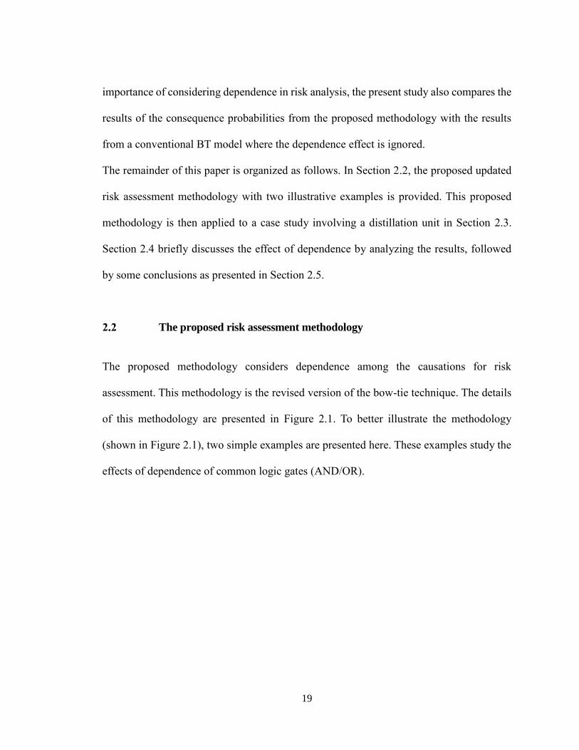
The proposed risk assessment methodology
The proposed methodology considers dependence among the causations for risk
assessment. This methodology is the revised version of the bow-tie technique. The details
of this methodology are presented in Figure 2.1. To better illustrate the methodology
(shown in Figure 2.1), two simple examples are presented here. These examples study the
effects of dependence of common logic gates (AND/OR).
20
Step 1: Identify accident scenario
Consider a process system
Step 5: Estimate the probability of major OEs
Step 2: Develop bow-tie model
Step 3: Derive occurrence probabilities of initiating events
(IEs) and failure probabilities of safety barriers (SBs)
Step 4: Estimate top event (TE) and outcome events (OEs)
probabilities considering interdependence of IEs and SBs
Figure 2.1 Methodology for risk assessment considering dependence.
Step 1: Identify accident scenario
Once a process system is selected, the probable accident scenario is developed.
Subsequently, the causes of this accident scenario or top event (TE), which are called
initiating events (IEs) in bow-tie analysis, are identified. The accident scenario is then
further analyzed based on the failure or success of safety barriers (SBs), leading to the
possible consequences or outcome events (OEs).
In the examples, a range of IEs (A, B, C and D) and two SBs (SB1 and SB2), the respective
TEs and OEs are identified. OE1 refers to safe condition, where both SB1 and SB2 function
21
despite TE occurs. If SB1 functions but SB2 fails, a near miss outcome event is viewed to
occur denoted by OE2. An incident (OE3) will occur once SB1 fails however SB2
fortunately works. Lastly, the worst OE is an accident (OE4), when neither SB1 nor SB2
succeeds in mitigating the outcome of TE.
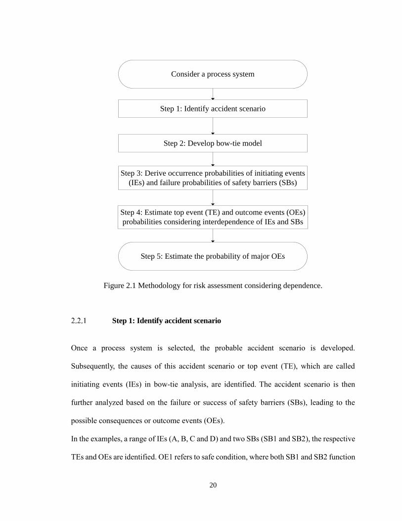
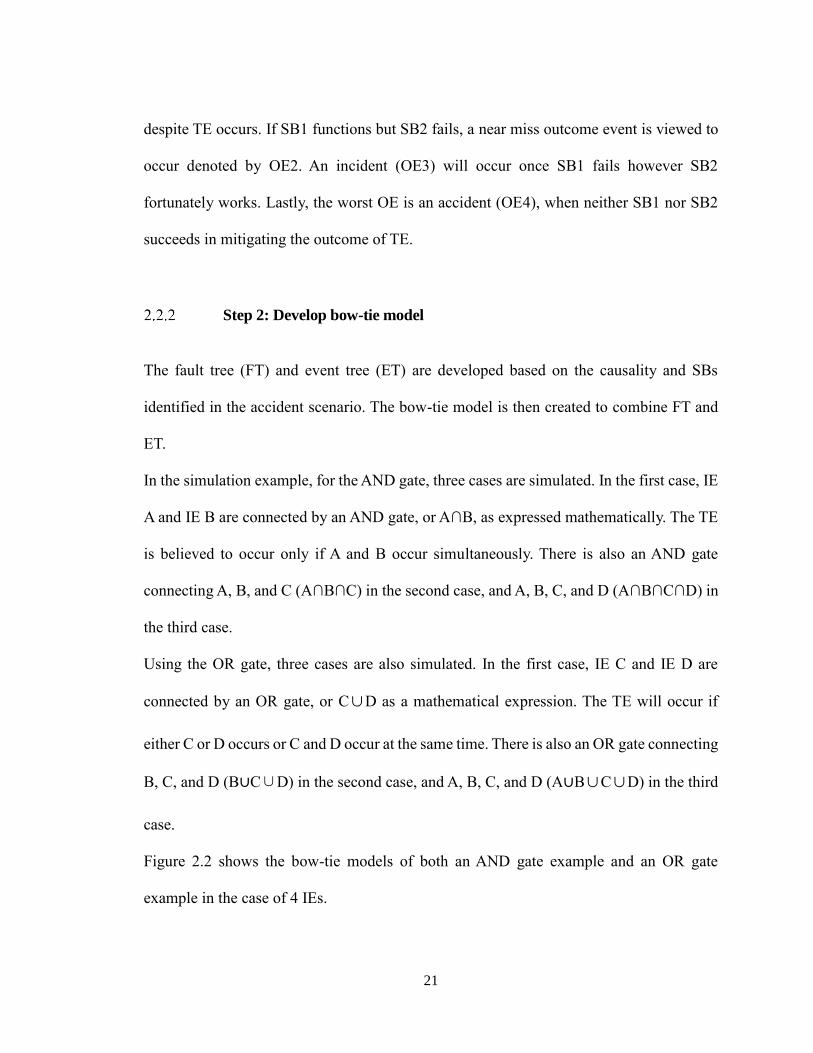
Step 2: Develop bow-tie model
The fault tree (FT) and event tree (ET) are developed based on the causality and SBs
identified in the accident scenario. The bow-tie model is then created to combine FT and
ET.
In the simulation example, for the AND gate, three cases are simulated. In the first case, IE
A and IE B are connected by an AND gate, or A∩B, as expressed mathematically. The TE
is believed to occur only if A and B occur simultaneously. There is also an AND gate
connecting A, B, and C (A∩B∩C) in the second case, and A, B, C, and D (A∩B∩C∩D) in
the third case.
Using the OR gate, three cases are also simulated. In the first case, IE C and IE D are
connected by an OR gate, or C∪D as a mathematical expression. The TE will occur if
either C or D occurs or C and D occur at the same time. There is also an OR gate connecting
B, C, and D (B∪C∪D) in the second case, and A, B, C, and D (A∪B∪C∪D) in the third
case.
Figure 2.2 shows the bow-tie models of both an AND gate example and an OR gate
example in the case of 4 IEs.
22
TE
AD
BC
SB1 SB2
Safe condition (OE1)
Near miss (OE2)
Incident (OE3)
Accident (OE4)
(a)
23
TE
AD
BC
SB1 SB2
Safe condition (OE1)
Near miss (OE2)
Incident (OE3)
Accident (OE4)
(b)
Figure 2.2 Bow-tie models of the example in the case of 4 IEs (A, B, C, and D) and two
logical operators: (a) AND gate; (b) OR gate.
Step 3: Derive occurrence probabilities of IEs and failure probabilities of
SBs
In a classical model, discrete values for probabilities are used to estimate the occurrence
probabilities of OEs. In contrast, it is assumed that IEs probabilities and failure
probabilities of SBs follow the Beta distribution, with selected parameters a and b in the
proposed model. The failure probability distribution function is given as:
f(x)∝xa-1 (1-x)b-1 (2.1)
The mean value is a/(a+b) and the variance is ab/[(a+b)2(a+b+1)]. The parameters are
selected such that the mean is equal to the discrete value of the IE probability or the failure
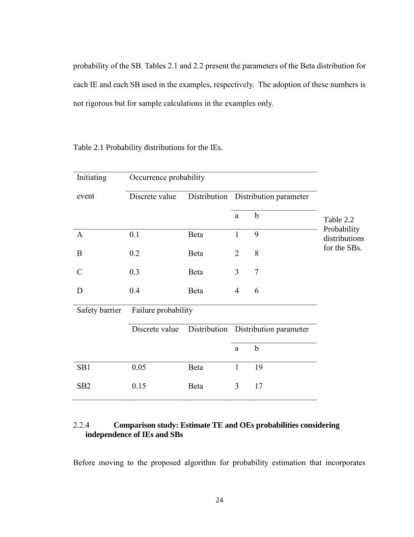
24
probability of the SB. Tables 2.1 and 2.2 present the parameters of the Beta distribution for
each IE and each SB used in the examples, respectively. The adoption of these numbers is
not rigorous but for sample calculations in the examples only.
Table 2.1 Probability distributions for the IEs.
Table 2.2
Probability
distributions
for the SBs.
Safety barrier Failure probability
Discrete value Distribution Distribution parameter
a b
SB1 0.05 Beta 1 19
SB2 0.15 Beta 3 17
Comparison study: Estimate TE and OEs probabilities considering
independence of IEs and SBs
Before moving to the proposed algorithm for probability estimation that incorporates
Initiating
event
Occurrence probability
Discrete value Distribution Distribution parameter
a b
A 0.1 Beta 1 9
B 0.2 Beta 2 8
C 0.3 Beta 3 7
D 0.4 Beta 4 6
25
interdependence, the traditional bow-tie method is first used for comparison purpose. It is
considered that the occurrence probabilities of IEs and the failure probabilities of SBs are
independent. Then the discrete occurrence probability of an OE is estimated as the discrete
probability of the TE multiplied by the discrete probabilities of failure or success of various
SBs along the corresponding branch. The probability of the TE is calculated as the union
of minimal cut sets.
For example, the discrete probabilities of TE and OE3 in Figure 2.2-a are as follows.
Pr(TE)=Pr(A).Pr(B).Pr(C).Pr(D) (2.2)
Pr(OE3)=Pr(TE). Pr(SB1).Pr(𝑆𝐵2̅̅ ̅̅ ̅) (2.3)
where Pr(A) and Pr(B) are the discrete probabilities of IE A and of IE B, and Pr(SB1) and
Pr(𝑆𝐵2̅̅ ̅̅ ̅) refer to the discrete failure and non-failure probability of safety barriers SB1 and
SB2, respectively. Other OEs probabilities are obtained similarly.
Step 4: Estimate TE and OEs probabilities considering interdependence of
IEs and SBs
Algorithm for probability estimation by Monte Carlo simulations
To capture the correlation among IEs and SBs, copula functions are used. A copula is a
multivariate probability distribution, where each random variable has a uniform marginal
distribution on the unit interval [0, 1]. Because of the possibility for dependence among
variables, a copula can be used to construct a new multivariate distribution for dependent
variables.
There are many kinds of multi-dimensional copulas. In this work, the Gaussian copula,

26
which is one of the most common copulas, is used. It is a simple yet flexible elliptical
copula. A correlation matrix consisting of corresponding correlation parameters (ρ) is then
designed according to the interactions among IEs and SBs.
Subsequently, Monte Carlo integration is conducted to simulate the probabilities. In each
trial, correlated random numbers with uniform distribution between 0 and 1 are first
generated and compared with the random numbers that follow specific Beta distributions
of corresponding IEs. If the uniform random number is smaller or equal to the random
number of the IE, the IE will occur. The next step is the analysis of the intermediate event.
If there is an AND gate connecting the IEs, the relative intermediate event will only occur
when all the corresponding IEs occur. In the case of an OR gate, the intermediate event
will occur when any corresponding IE occurs. By applying this analysis of the AND gate
as well as the OR gate to the following intermediate events in the bow-tie model, whether
the TE will occur or not in this trial can be finally confirmed.
The right side of the bow-tie model, which is the ET, is then analyzed. Similar to the
simulation of IEs, correlated random numbers are generated from the copula function that
is applied to SBs. The results for which SBs fail in this trial can be derived by comparing
these numbers with the random numbers that represent failure probabilities of respective
SBs. These results determine the branch of the ET that points to the particular OE. This
simulation is conducted for a million trials. The mean occurrence probabilities of the TE
along with all the OEs are obtained.
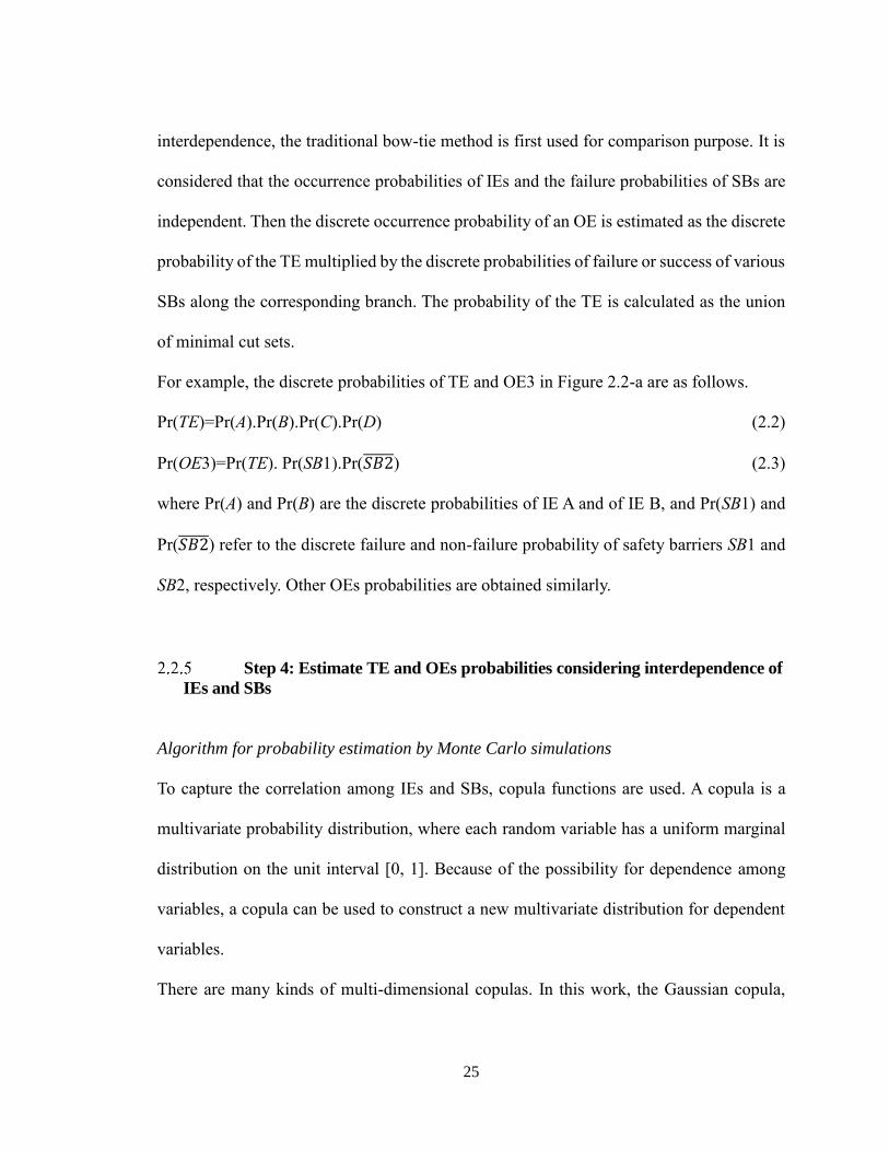
For the sake of simplicity, the correlation parameters of any two IEs in the examples are
assumed to be identical, starting from 0.2 to 1. One of the correlation matrices used in the
27
case of A∩B∩C is shown in Table 2.3.
Monte Carlo simulations with one million trials are conducted for the two examples. The
correlation parameters used and the resulting mean occurrence probabilities of the TEs for
both independent and interdependent cases are presented in Figures 3.3 and 3.4, where ρ
being 0 signifies that the IEs are completely independent therefore the probabilities are
calculated by use of the method discussed in Section 2.2.4, where ρ = 1 signifies that the
IEs are deterministically related, while other correlation parameters that fall between 0 and
1 signify that the IEs are partly dependent.
Table 2.3 One of the correlation matrices for the case A∩B∩C.
pA pB pC
pA 1 0.8 0.8
pB 0.8 1 0.8
pC 0.8 0.8 1
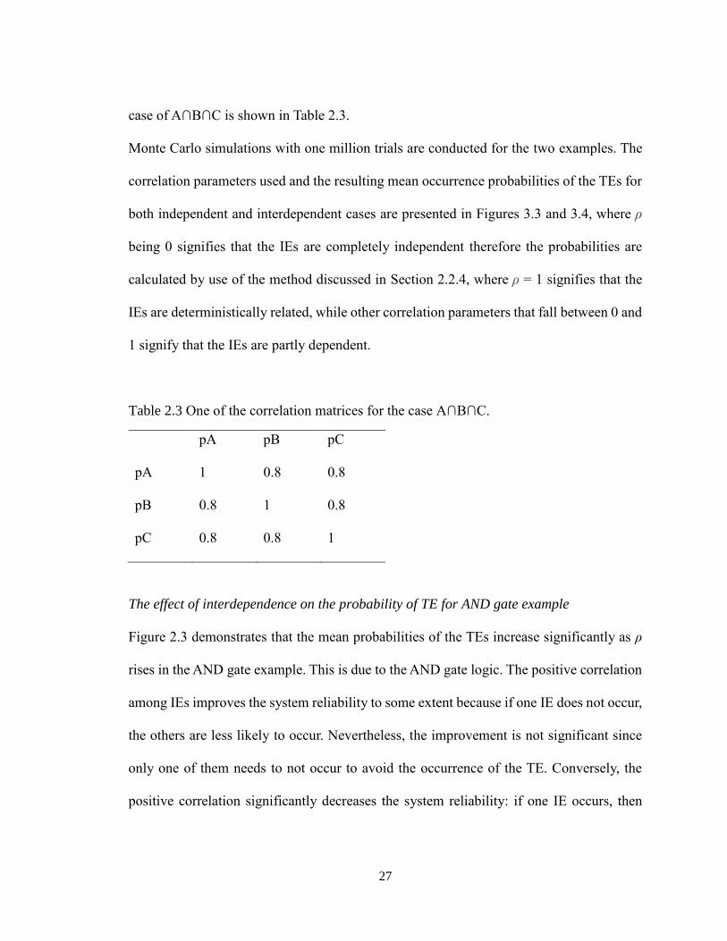
The effect of interdependence on the probability of TE for AND gate example
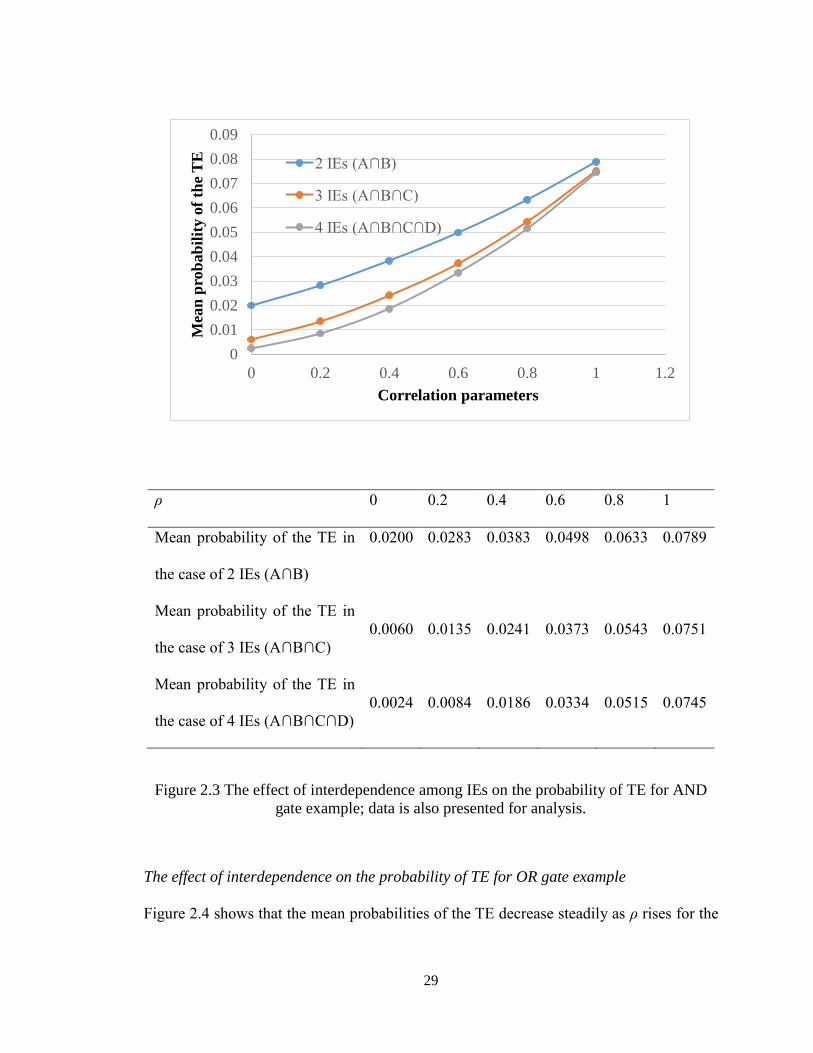
Figure 2.3 demonstrates that the mean probabilities of the TEs increase significantly as ρ
rises in the AND gate example. This is due to the AND gate logic. The positive correlation
among IEs improves the system reliability to some extent because if one IE does not occur,
the others are less likely to occur. Nevertheless, the improvement is not significant since
only one of them needs to not occur to avoid the occurrence of the TE. Conversely, the
positive correlation significantly decreases the system reliability: if one IE occurs, then
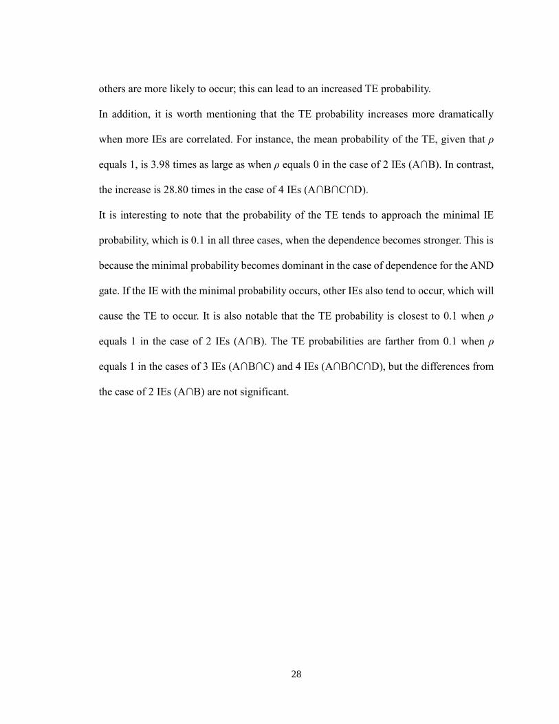
28
others are more likely to occur; this can lead to an increased TE probability.
In addition, it is worth mentioning that the TE probability increases more dramatically
when more IEs are correlated. For instance, the mean probability of the TE, given that ρ
equals 1, is 3.98 times as large as when ρ equals 0 in the case of 2 IEs (A∩B). In contrast,
the increase is 28.80 times in the case of 4 IEs (A∩B∩C∩D).
It is interesting to note that the probability of the TE tends to approach the minimal IE
probability, which is 0.1 in all three cases, when the dependence becomes stronger. This is
because the minimal probability becomes dominant in the case of dependence for the AND
gate. If the IE with the minimal probability occurs, other IEs also tend to occur, which will
cause the TE to occur. It is also notable that the TE probability is closest to 0.1 when ρ
equals 1 in the case of 2 IEs (A∩B). The TE probabilities are farther from 0.1 when ρ
equals 1 in the cases of 3 IEs (A∩B∩C) and 4 IEs (A∩B∩C∩D), but the differences from
the case of 2 IEs (A∩B) are not significant.
29
ρ 0 0.2 0.4 0.6 0.8 1
Mean probability of the TE in
the case of 2 IEs (A∩B)
0.0200 0.0283 0.0383 0.0498 0.0633 0.0789
Mean probability of the TE in
the case of 3 IEs (A∩B∩C)
0.0060 0.0135 0.0241 0.0373 0.0543 0.0751
Mean probability of the TE in
the case of 4 IEs (A∩B∩C∩D)
0.0024 0.0084 0.0186 0.0334 0.0515 0.0745
Figure 2.3 The effect of interdependence among IEs on the probability of TE for AND
gate example; data is also presented for analysis.
The effect of interdependence on the probability of TE for OR gate example
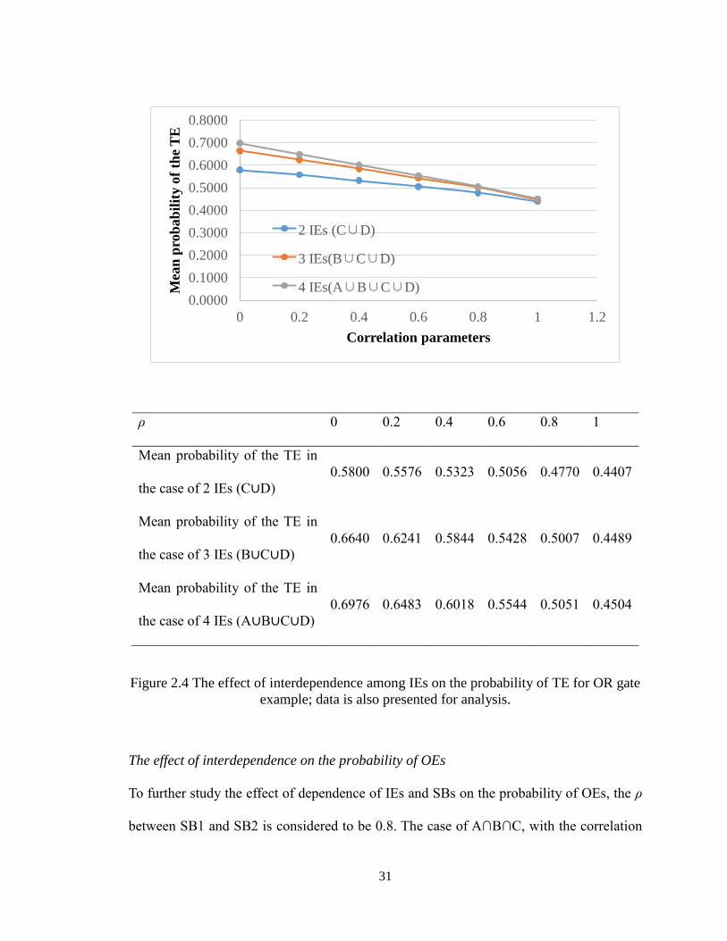
Figure 2.4 shows that the mean probabilities of the TE decrease steadily as ρ rises for the
0
0.01
0.02
0.03
0.04
0.05
0.06
0.07
0.08
0.09
0 0.2 0.4 0.6 0.8 1 1.2
Mea
n p
rob
ab
ilit
y o
f th
e T
E
Correlation parameters
2 IEs (A∩B)
3 IEs (A∩B∩C)
4 IEs (A∩B∩C∩D)
30
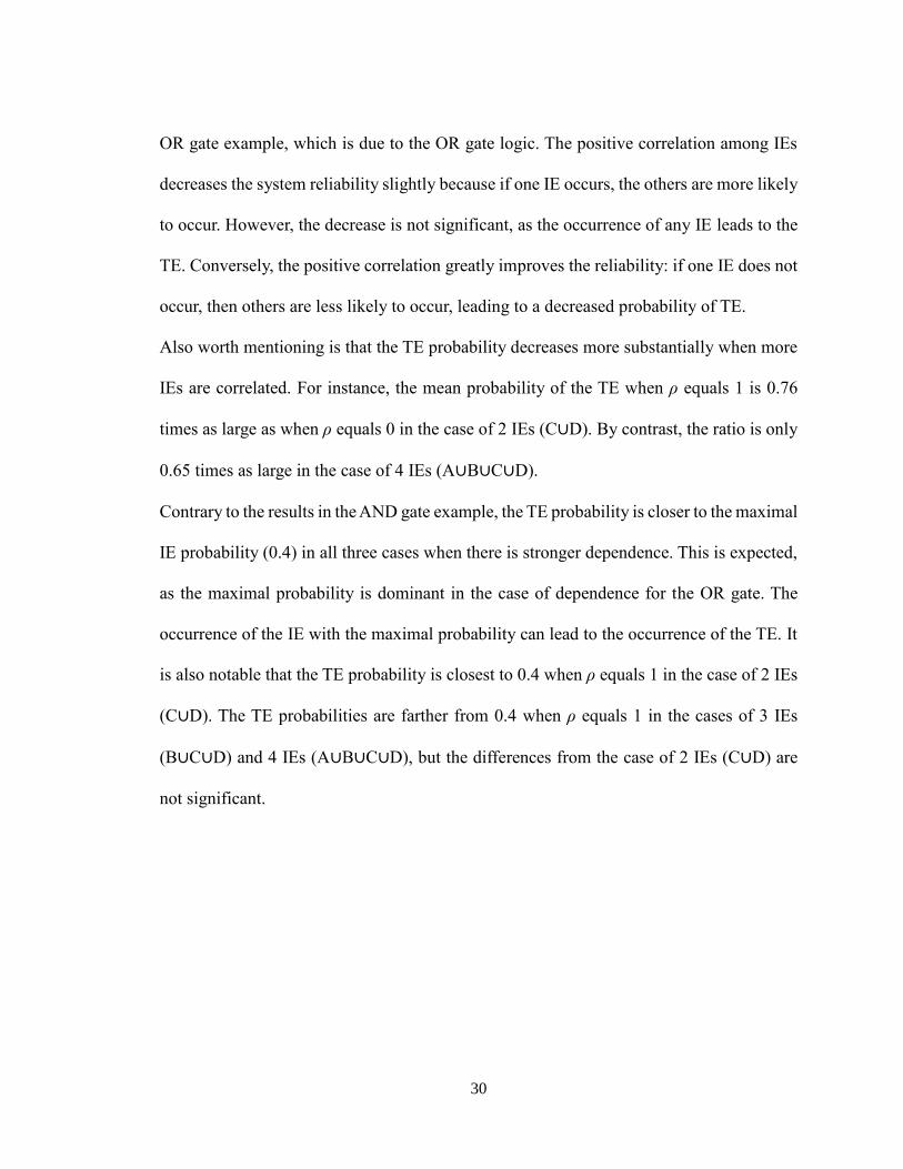
OR gate example, which is due to the OR gate logic. The positive correlation among IEs
decreases the system reliability slightly because if one IE occurs, the others are more likely
to occur. However, the decrease is not significant, as the occurrence of any IE leads to the
TE. Conversely, the positive correlation greatly improves the reliability: if one IE does not
occur, then others are less likely to occur, leading to a decreased probability of TE.
Also worth mentioning is that the TE probability decreases more substantially when more
IEs are correlated. For instance, the mean probability of the TE when ρ equals 1 is 0.76
times as large as when ρ equals 0 in the case of 2 IEs (C∪D). By contrast, the ratio is only
0.65 times as large in the case of 4 IEs (A∪B∪C∪D).
Contrary to the results in the AND gate example, the TE probability is closer to the maximal
IE probability (0.4) in all three cases when there is stronger dependence. This is expected,
as the maximal probability is dominant in the case of dependence for the OR gate. The
occurrence of the IE with the maximal probability can lead to the occurrence of the TE. It
is also notable that the TE probability is closest to 0.4 when ρ equals 1 in the case of 2 IEs
(C∪D). The TE probabilities are farther from 0.4 when ρ equals 1 in the cases of 3 IEs
(B∪C∪D) and 4 IEs (A∪B∪C∪D), but the differences from the case of 2 IEs (C∪D) are
not significant.
31
ρ 0 0.2 0.4 0.6 0.8 1
Mean probability of the TE in
the case of 2 IEs (C∪D)
0.5800 0.5576 0.5323 0.5056 0.4770 0.4407
Mean probability of the TE in
the case of 3 IEs (B∪C∪D)
0.6640 0.6241 0.5844 0.5428 0.5007 0.4489
Mean probability of the TE in
the case of 4 IEs (A∪B∪C∪D)
0.6976 0.6483 0.6018 0.5544 0.5051 0.4504
Figure 2.4 The effect of interdependence among IEs on the probability of TE for OR gate
example; data is also presented for analysis.
The effect of interdependence on the probability of OEs
To further study the effect of dependence of IEs and SBs on the probability of OEs, the ρ
between SB1 and SB2 is considered to be 0.8. The case of A∩B∩C, with the correlation
0.0000
0.1000
0.2000
0.3000
0.4000
0.5000
0.6000
0.7000
0.8000
0 0.2 0.4 0.6 0.8 1 1.2
Mea
n p
rob
ab
ilit
y o
f th
e T
E
Correlation parameters
2 IEs (C∪D)
3 IEs(B∪C∪D)
4 IEs(A∪B∪C∪D)
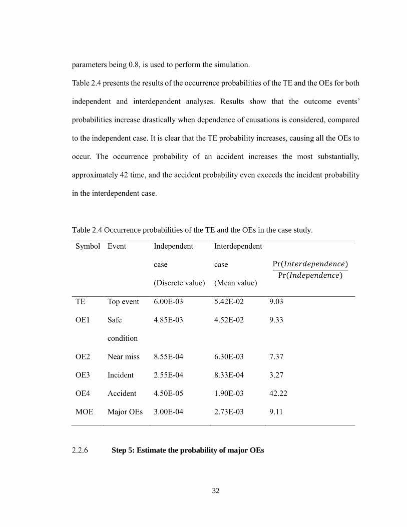
32
parameters being 0.8, is used to perform the simulation.
Table 2.4 presents the results of the occurrence probabilities of the TE and the OEs for both
independent and interdependent analyses. Results show that the outcome events’
probabilities increase drastically when dependence of causations is considered, compared
to the independent case. It is clear that the TE probability increases, causing all the OEs to
occur. The occurrence probability of an accident increases the most substantially,
approximately 42 time, and the accident probability even exceeds the incident probability
in the interdependent case.
Table 2.4 Occurrence probabilities of the TE and the OEs in the case study.
Symbol Event Independent
case
(Discrete value)
Interdependent
case
(Mean value)
Pr(𝐼𝑛𝑡𝑒𝑟𝑑𝑒𝑝𝑒𝑛𝑑𝑒𝑛𝑐𝑒)
Pr(𝐼𝑛𝑑𝑒𝑝𝑒𝑛𝑑𝑒𝑛𝑐𝑒)
TE Top event 6.00E-03 5.42E-02 9.03
OE1 Safe
condition
4.85E-03 4.52E-02 9.33
OE2 Near miss 8.55E-04 6.30E-03 7.37
OE3 Incident 2.55E-04 8.33E-04 3.27
OE4 Accident 4.50E-05 1.90E-03 42.22
MOE Major OEs 3.00E-04 2.73E-03 9.11
Step 5: Estimate the probability of major OEs
33
Major outcome events are defined as those consequences that cause severe loss, including
fatalities or significant financial loss. In this case, incident (OE3) and accident (OE4) are
considered to be major OEs. The probability of major OEs is estimated by combining the
probability of OE3 and OE4. Results are presented in Table 2.4. It is clear that the
occurrence probability of major OEs in the interdependent case is much larger than the
probability in the independent case.
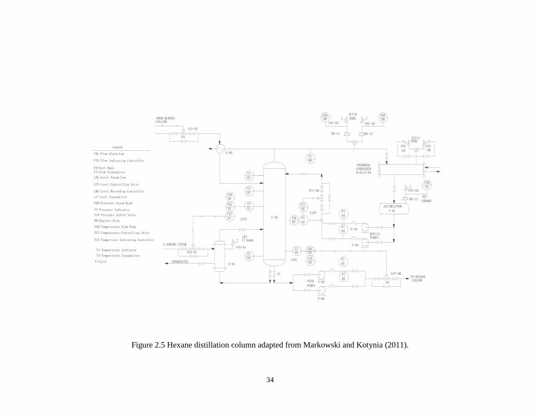
Application of the proposed methodology
To test and verify the proposed methodology, a detailed case study is conducted. The
methodology is applied to an accident scenario in a hexane distillation unit, adopted from
a study by Markowski and Kotynia (2011). The installation is presented in Figure 2.5.
34
TI02
TI03
TT01
TAH01
TAL01
TIC01
TI04
LT05
LRC05
LAL05
PI07
PI04
PI03
FIC02
FAL02
FT02
PAH09
PAH09
PI08
PAH10
PI06
C-01SIST
SISF
FCV-02
FROM QUENCHCOLLIMN
LCV-02
FO
E-02
PSV-02
RD-11
BARGSET10
PSV-03
RD-12SET14BARG
PSV
-05
PSV-06
OVERHEADCONDENSERD-03/E-04
PSV-04
RD-13SET10BARG
ACCUMULATOR
V-01
P-04
REFLUXPUMPS
P-03
SISL
FEED
PUMPSP-07
P-06
LCV-06
Legend
FO
TO HEXANECOLUMN
SET17 BARG
PSV-01
E-01
FAL-Flow Alarm Low
FIC-Flow Indicating Controller
FO-Fail OpenFT-Flow Transmitter
LAL-Level Alarm Low
LCV-Level Controlling Valve
LRC-Level Recording Controller
LT-level Transmitter
PAH-Pressure Alarm High
PI-Pressure Indicator
PSV-Pressure Safety Valve
RD-Rupture Disk
TAH-Temperature Alam High
TCV-Temperature Controlling Valve
TIC-Temperture Indicating Controller
TI-Temperature Indicator
TT-Temperature Transmitter
V-Valve
3,45BARG STEAM
TCV-01
CONDENSATE
V1
Figure 2.5 Hexane distillation column adapted from Markowski and Kotynia (2011).
35
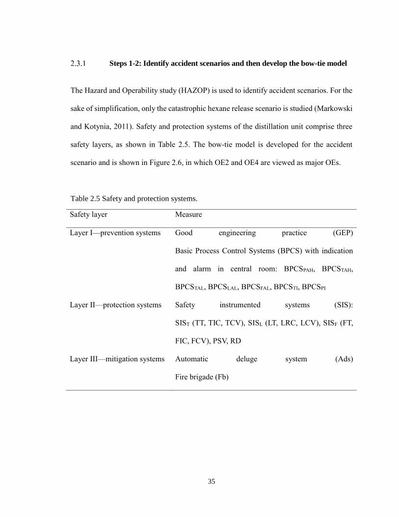
Steps 1-2: Identify accident scenarios and then develop the bow-tie model
The Hazard and Operability study (HAZOP) is used to identify accident scenarios. For the
sake of simplification, only the catastrophic hexane release scenario is studied (Markowski
and Kotynia, 2011). Safety and protection systems of the distillation unit comprise three
safety layers, as shown in Table 2.5. The bow-tie model is developed for the accident
scenario and is shown in Figure 2.6, in which OE2 and OE4 are viewed as major OEs.
Table 2.5 Safety and protection systems.
Safety layer Measure
Layer I—prevention systems Good engineering practice (GEP)
Basic Process Control Systems (BPCS) with indication
and alarm in central room: BPCSPAH, BPCSTAH,
BPCSTAL, BPCSLAL, BPCSFAL, BPCSTI, BPCSPI
Layer II—protection systems Safety instrumented systems (SIS):
SIST (TT, TIC, TCV), SISL (LT, LRC, LCV), SISF (FT,
FIC, FCV), PSV, RD
Layer III—mitigation systems Automatic deluge system (Ads)
Fire brigade (Fb)
36
G
H
C
Condenser failure
Loss of cooling
I
J
Failure of control systems
E
D
Overheating Overpressure
K
L
F
Outflow blockage
Overfilling
A
B
Failure of over-pressure protect
N
M
Mechanical failure
O
Process upset failure
Cata
str
op
hic
h
ex
an
e r
ele
ase
Fire extinguished (OE1)
Fire extinguished (OE1)
Pool fire and fatalities (OE2)
Pool fire (OE2b)
Spill / dispersion (OE3)
VCE / FF and fatalities (OE4)
Vapour cloud explosion / flash
fire (OE4b)
Spill / dispersion (OE3)
Initiating event (IE) Intermediate event (IE) Top event (TE) Conditioning event (CE)
Safety function (SF) enCE Outcome event (OE)
Imm
ed
iate
ig
nit
ion
Late
ig
nit
ion
Au
tom
ati
c
delu
ge s
yste
m
Fata
liti
es i
n
ex
po
sed
are
a
Fir
e b
rig
ad
e
Yes
YesYes
Yes
Yes
Yes
Yes
No
No
No
No
No
No
No
Figure 2.6 Bow-tie accident scenario model for Hexane distillation example similar to
one reported in (Markowski and Kotynia, 2011).
Step 3: Derive occurrence probabilities of IEs and failure probabilities of
SBs
The probability numbers for the conditioning events (CEs) as well as the safety functions
(SFs) and the IEs are presented in Tables 2.6 and 2.7 respectively. It is notable that
Markowski and Kotynia (2011) used fuzzy probability numbers for the IEs and standard
probability numbers for the CEs, based on look-up tables developed in the LOPA book
(CCPS, 2001) and experts’ knowledge and experience. The failure probabilities for the SFs
are assumed based on experts’ judgement because they are not given in Markowski and
37
Kotynia (2011). In addition, all the probabilities are considered to follow Beta distribution
with corresponding parameters.
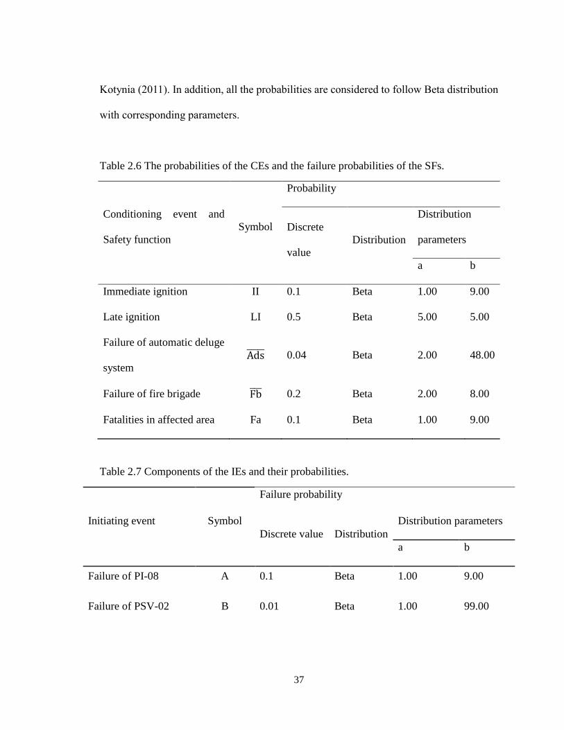
Table 2.6 The probabilities of the CEs and the failure probabilities of the SFs.
Conditioning event and
Safety function
Symbol
Probability
Discrete
value
Distribution
Distribution
parameters
a b
Immediate ignition II 0.1 Beta 1.00 9.00
Late ignition LI 0.5 Beta 5.00 5.00
Failure of automatic deluge
system Ads̅̅ ̅̅ ̅ 0.04 Beta 2.00 48.00
Failure of fire brigade Fb̅̅ ̅ 0.2 Beta 2.00 8.00
Fatalities in affected area Fa 0.1 Beta 1.00 9.00
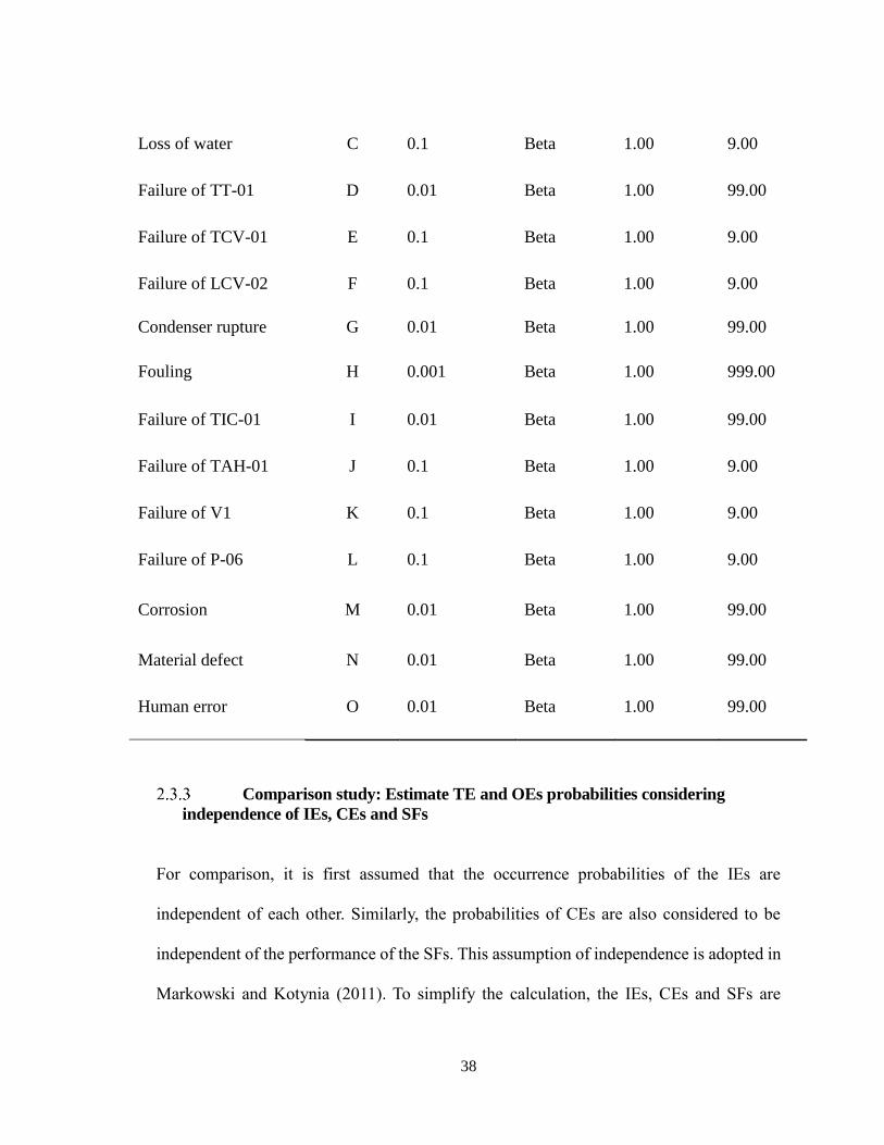
Table 2.7 Components of the IEs and their probabilities.
Initiating event Symbol
Failure probability
Discrete value Distribution
Distribution parameters
a b
Failure of PI-08 A 0.1 Beta 1.00 9.00
Failure of PSV-02 B 0.01 Beta 1.00 99.00
38
Loss of water C 0.1 Beta 1.00 9.00
Failure of TT-01 D 0.01 Beta 1.00 99.00
Failure of TCV-01 E 0.1 Beta 1.00 9.00
Failure of LCV-02 F 0.1 Beta 1.00 9.00
Condenser rupture G 0.01 Beta 1.00 99.00
Fouling H 0.001 Beta 1.00 999.00
Failure of TIC-01 I 0.01 Beta 1.00 99.00
Failure of TAH-01 J 0.1 Beta 1.00 9.00
Failure of V1 K 0.1 Beta 1.00 9.00
Failure of P-06 L 0.1 Beta 1.00 9.00
Corrosion M 0.01 Beta 1.00 99.00
Material defect N 0.01 Beta 1.00 99.00
Human error O 0.01 Beta 1.00 99.00
Comparison study: Estimate TE and OEs probabilities considering
independence of IEs, CEs and SFs
For comparison, it is first assumed that the occurrence probabilities of the IEs are
independent of each other. Similarly, the probabilities of CEs are also considered to be
independent of the performance of the SFs. This assumption of independence is adopted in
Markowski and Kotynia (2011). To simplify the calculation, the IEs, CEs and SFs are
39
designated discrete probability numbers.
To derive the discrete probabilities of the TE and the OEs, one can adopt the method
discussed in Section 2.2.4. In this case, for example, the probabilities of TE and OE2 are
calculated as shown in the equations below:
Pr(TE)=Pr(A)Pr(B)Pr(C)+Pr(A)Pr(B)Pr(G)+Pr(A)Pr(B)Pr(H)+Pr(A)Pr(B)Pr(D)+Pr(A)Pr(B
)Pr(E)+Pr(A)Pr(B)Pr(I)Pr(J)+Pr(A)Pr(B)Pr(F)Pr(K)+Pr(A)Pr(B)Pr(F)Pr(L)+Pr(M)+Pr(N)
+Pr(O) (2.4)
Pr(OE2)=Pr(TE)Pr(II)Pr(𝐴𝑑𝑠̅̅ ̅̅ ̅)Pr(𝐹𝑏̅̅̅̅ )Pr(Fa) (2.5)
where Pr(A), Pr(B),…, Pr(Fa) stand for the respective discrete probabilities in Tables 2.6
and 2.7. All other OEs probabilities are obtained similarly. The discrete probability values
of the TE and the OEs are summarized in Table 2.10.
Step 4: Estimate TE and OEs probabilities considering interdependence of
IEs, CEs and SFs
To demonstrate the advantage of the proposed methodology, the dependence among the
IEs, CEs and SFs is considered in this case study. As Table 2.8 shows, B, E, F, and K are
assumed to be correlated because they are all concerned with the failure of valves. However,
the ρ between the failure of the temperature controlling valve (E) and the failure of the
level controlling valve (F) is assumed to be 0.8. The ρ between the failure of the pressure
safety valve (B) and the failure of valve 1 (K) is also considered to be 0.8. The ρ between
B and E, B and F, E and K, or F and K is considered to be 0.6. In addition, it is assumed
that the failure of the pressure indicator (A) and the failure of the pressure safety valve (B)
40
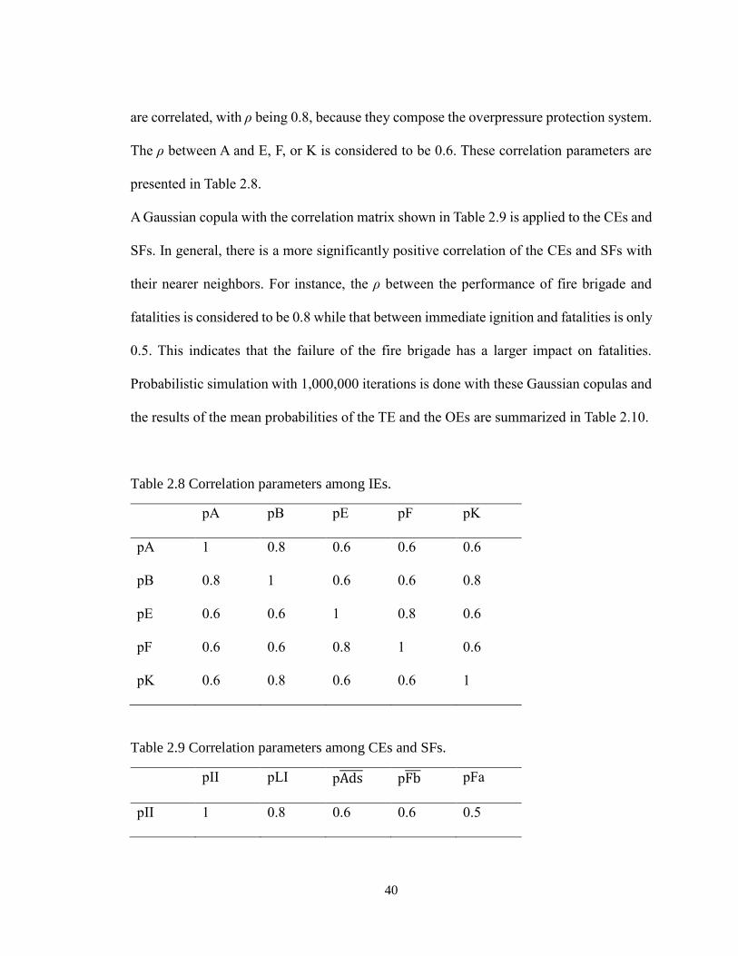
are correlated, with ρ being 0.8, because they compose the overpressure protection system.
The ρ between A and E, F, or K is considered to be 0.6. These correlation parameters are
presented in Table 2.8.
A Gaussian copula with the correlation matrix shown in Table 2.9 is applied to the CEs and
SFs. In general, there is a more significantly positive correlation of the CEs and SFs with
their nearer neighbors. For instance, the ρ between the performance of fire brigade and
fatalities is considered to be 0.8 while that between immediate ignition and fatalities is only
0.5. This indicates that the failure of the fire brigade has a larger impact on fatalities.
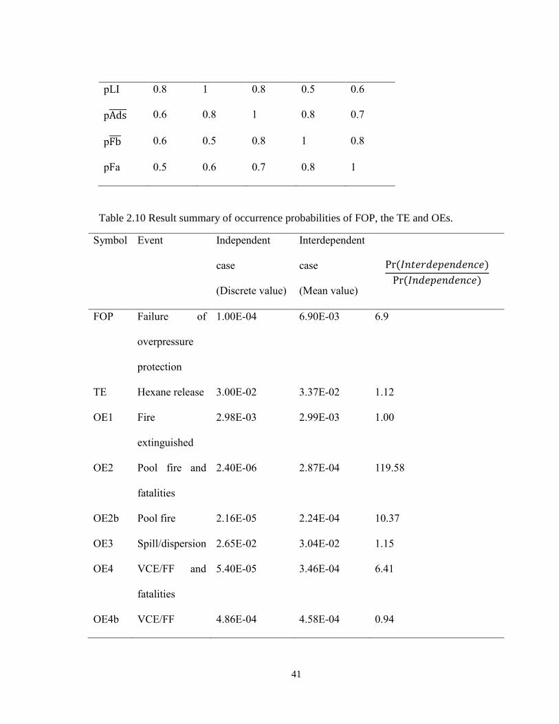
Probabilistic simulation with 1,000,000 iterations is done with these Gaussian copulas and
the results of the mean probabilities of the TE and the OEs are summarized in Table 2.10.
Table 2.8 Correlation parameters among IEs.
pA pB pE pF pK
pA 1 0.8 0.6 0.6 0.6
pB 0.8 1 0.6 0.6 0.8
pE 0.6 0.6 1 0.8 0.6
pF 0.6 0.6 0.8 1 0.6
pK 0.6 0.8 0.6 0.6 1
Table 2.9 Correlation parameters among CEs and SFs.
pII pLI pAds̅̅ ̅̅ ̅ pFb̅̅ ̅ pFa
pII 1 0.8 0.6 0.6 0.5
41
pLI 0.8 1 0.8 0.5 0.6
pAds̅̅ ̅̅ ̅ 0.6 0.8 1 0.8 0.7
pFb̅̅ ̅ 0.6 0.5 0.8 1 0.8
pFa 0.5 0.6 0.7 0.8 1
Table 2.10 Result summary of occurrence probabilities of FOP, the TE and OEs.
Symbol Event Independent
case
(Discrete value)
Interdependent
case
(Mean value)
Pr(𝐼𝑛𝑡𝑒𝑟𝑑𝑒𝑝𝑒𝑛𝑑𝑒𝑛𝑐𝑒)
Pr(𝐼𝑛𝑑𝑒𝑝𝑒𝑛𝑑𝑒𝑛𝑐𝑒)
FOP Failure of
overpressure
protection
1.00E-04 6.90E-03 6.9
TE Hexane release 3.00E-02 3.37E-02 1.12
OE1 Fire
extinguished
2.98E-03 2.99E-03 1.00
OE2 Pool fire and
fatalities
2.40E-06 2.87E-04 119.58
OE2b Pool fire 2.16E-05 2.24E-04 10.37
OE3 Spill/dispersion 2.65E-02 3.04E-02 1.15
OE4 VCE/FF and
fatalities
5.40E-05 3.46E-04 6.41
OE4b VCE/FF 4.86E-04 4.58E-04 0.94
42
MOE Major OEs
where fatalities
occur
5.64E-05 6.33E-04 11.22
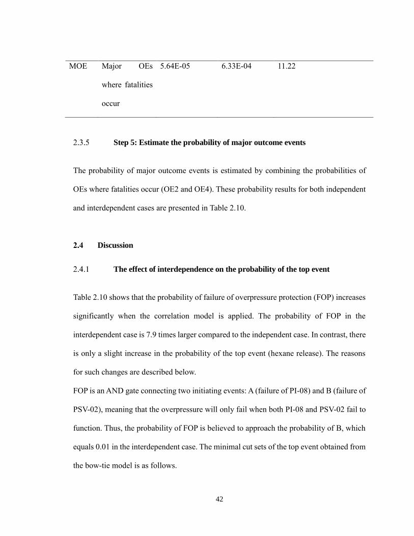
Step 5: Estimate the probability of major outcome events
The probability of major outcome events is estimated by combining the probabilities of
OEs where fatalities occur (OE2 and OE4). These probability results for both independent
and interdependent cases are presented in Table 2.10.
Discussion
The effect of interdependence on the probability of the top event
Table 2.10 shows that the probability of failure of overpressure protection (FOP) increases
significantly when the correlation model is applied. The probability of FOP in the
interdependent case is 7.9 times larger compared to the independent case. In contrast, there
is only a slight increase in the probability of the top event (hexane release). The reasons
for such changes are described below.
FOP is an AND gate connecting two initiating events: A (failure of PI-08) and B (failure of
PSV-02), meaning that the overpressure will only fail when both PI-08 and PSV-02 fail to
function. Thus, the probability of FOP is believed to approach the probability of B, which
equals 0.01 in the interdependent case. The minimal cut sets of the top event obtained from
the bow-tie model is as follows.
43
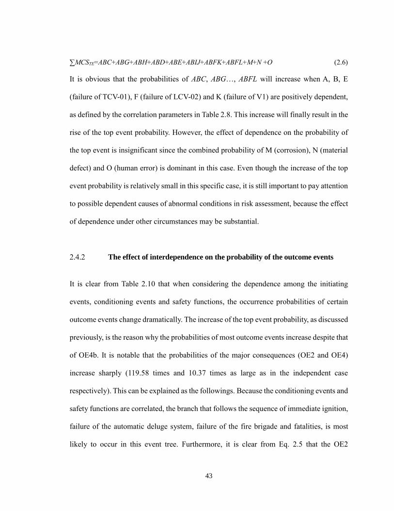
∑MCSTE=ABC+ABG+ABH+ABD+ABE+ABIJ+ABFK+ABFL+M+N +O (2.6)
It is obvious that the probabilities of ABC, ABG…, ABFL will increase when A, B, E
(failure of TCV-01), F (failure of LCV-02) and K (failure of V1) are positively dependent,
as defined by the correlation parameters in Table 2.8. This increase will finally result in the
rise of the top event probability. However, the effect of dependence on the probability of
the top event is insignificant since the combined probability of M (corrosion), N (material
defect) and O (human error) is dominant in this case. Even though the increase of the top
event probability is relatively small in this specific case, it is still important to pay attention
to possible dependent causes of abnormal conditions in risk assessment, because the effect
of dependence under other circumstances may be substantial.
The effect of interdependence on the probability of the outcome events
It is clear from Table 2.10 that when considering the dependence among the initiating
events, conditioning events and safety functions, the occurrence probabilities of certain
outcome events change dramatically. The increase of the top event probability, as discussed
previously, is the reason why the probabilities of most outcome events increase despite that
of OE4b. It is notable that the probabilities of the major consequences (OE2 and OE4)
increase sharply (119.58 times and 10.37 times as large as in the independent case
respectively). This can be explained as the followings. Because the conditioning events and
safety functions are correlated, the branch that follows the sequence of immediate ignition,
failure of the automatic deluge system, failure of the fire brigade and fatalities, is most
likely to occur in this event tree. Furthermore, it is clear from Eq. 2.5 that the OE2
44
probability tends to approach the top event probability multiplied by the minimal
occurrence probability among conditioning events and safety functions. Therefore, the
probability of OE2 increases most substantially. Similarly, the probabilities of OE2b and
OE4 both increase greatly, but the increase is not as large as OE2. Conversely, the
probability of OE4b decreases.
Table 2.10 also shows that the effect of dependence on outcome events probabilities is
more prominent than that of a top event probability. This indicates that the correlated safety
barriers have significant impacts on the occurrence probabilities of outcome events. If
feasible, it is suggested that independent barriers be added into safety systems.
Conclusions
This work has revised the bow-tie analysis by integrating the dependence among causation
factors. The revised bow-tie model, when run in probabilistic mode using Monte Carlo
simulations, provides more reliable and robust results. This is established revisiting a past
case study and comparing the results. The considerable difference between the respective
results reveals that the effect of dependence is significant and thus should be considered
when assessing risks of a process system.
The revised methodology is a simple adoption of the copula function to represent the
dependency. This revised methodology serves as a useful and easy to adopt tool to analyze
risk in a process system. It has the ability to model a complex engineering system where
dependencies are inherent. Another important feature of the revision is its ability to capture
and represent dependencies among the safety barriers and most importantly, to represent a
45
common failure model. This work could further be improved by transforming the bow-tie
into a network-based approach such as a Bayesian network or the Petri net along with
dependence modeling, using the copula function.
References
CCPS, 2001. Layer of Protection Analysis - Simplified Process Risk Assessment. AIChE
Durante, F. and Sempi, C., 2015. Principles of Copula Theory. CRC Press, Boca Raton,
FL.
Elidan, G., 2010. Copula Bayesian networks. , Neural Information Processing Systems
(NIPS).
Hashemi, S.J., Ahmed, S., Khan, F., 2015. Operational loss modelling for process
facilities using multivariate loss functions. Chem. Eng. Res. Design 104, 333-345.
Hashemi, S.J., Khan, F., Ahmed, S., 2016. Multivariate probabilistic safety analysis of
process facilities using the Copula Bayesian Network model. Computers and Chemical
Engineering 93, 128-142.
Khakzad, N., Khan, F., Amyotte, P., 2013. Dynamic safety analysis of process systems
by mapping bow-tie into Bayesian network. Process Safety and Environmental Protection
91, 46-53.
46
Khan, F.I., Haddara, M.R., 2004. Risk-based maintenance of ethylene oxide production
facilities. J. Hazard. Mater. 108, 147-159.
Khan, F.I., Sadiq, R., Husain, T., 2002. Risk-based process safety assessment and control
measures design for offshore process facilities. J. Hazard. Mater. 94, 1-36.
Markowski, A.S., Kotynia, A., 2011. "Bow-tie" model in layer of protection analysis.
Process Saf. Environ. Prot. 89, 205-213.
Meel, A., Seider, W.D., 2006. Plant-specific dynamic failure assessment using Bayesian
theory. Chemical Engineering Science 61, 7036-7056.
Mohseni Ahooyi, T., Arbogast, J.E., Soroush, M., 2014. Applications of the rolling pin
method. 1. An efficient alternative to Bayesian network modeling and inference.
Industrial and Engineering Chemistry Research 54, 4316-4325.
Nelsen, R.B., 2006. An Introduction to Copulas, Second Edition.. ed. New York, NY :
Springer New York.
Oktem, U.G., Seider, W.D., Soroush, M., Pariyani, A., 2013. Improve process safety with
near-miss analysis. Chem. Eng. Prog. 109, 20-27.
Pariyani, A., Seider, W.D., Oktem, U.G., Soroush, M., 2012. Dynamic risk analysis using
alarm databases to improve process safety and product quality: Part II-Bayesian analysis.
AIChE J. 58, 826-841.
47
Yi, W., Bier, V.M., 1998. An Application of Copulas to Accident Precursor Analysis.
Management Science 44, S257-S270.
Yu, H., Khan, F., Garaniya, V., 2015. A probabilistic multivariate method for fault
diagnosis of industrial processes. Chem. Eng. Res. Design 104, 306-318.
48
Chapter 3. Copula-based Bayesian network model for process system
risk assessment2
Abstract
Risk assessment is an essential exercise for process systems from early conceptual design
to operation and subsequently during decommissioning. Risk assessment methods have
evolved over the past two decades from index-based methods to detailed quantitative
methods. The Bayesian network (BN) is a recently developed technique used for risk
assessment that utilizes updating, adapting and discrete-time-based analysis properties.
Although the BN is a powerful technique, it continues to face the challenge of modelling
non-linear complex correlations of process components. This paper proposes a copula-
based Bayesian network model that assists in overcoming the challenge of non-linear
relationships. In addition to defining conditional probabilities, the copulas are also used to
describe the joint probability densities of the network nodes in the BN. Application of the
proposed model is demonstrated using a process accident case study. The results reveal that
the proposed model is effective in estimating more reliable accident probabilities. A
sensitivity analysis is also conducted to identify important factors that need to be monitored
to prevent accident occurrence. Though the focus of the present study is on process systems,
the proposed model is applicable to most engineering systems.
Key words: Risk assessment; Bayesian network; Dependence; Copula; Process safety;
Accident model
2 C.Guo et al. Submitted in revised form to Process Safety and Environmental Protection.
49
Introduction
Process industries deal with hazardous substances in large quantities. The release of these
materials can result in severe consequences including the loss of life, environmental
damage, and financial losses. As the nature of process operation is becoming more complex
due to process integration and digitalization, process safety management is becoming a key
concern, and risk assessment is an important step in process safety management. Many
approaches are available to conduct risk analyses of process systems. Among them, Layer
of Protection Analysis (LOPA) is a comprehensive yet easy-to-use risk assessment
technique. LOPA is a semi-quantitative approach which considers three layers of safety and
protection systems. The first layer is prevention systems, including Basic Process Control
Systems (BPCS) with indicators and alarms; the second layer consists of Safety
Instrumented Systems (SIS), while the third layer refers to mitigation systems such as the
deluge system (CCPS, 2001). CCPS (2001) has proposed a range of occurrence (or failure
on demand) probabilities of these systems. These probabilities are derived from plant data
and expert judgement.
Although LOPA is a recommended approach and widely used, it has some inherent
limitations. For instance, the causal analysis of an accident is too simple, and the predicted
probability is vague and often unrealistic.
As an alternative, the Quantitative Risk Analysis (QRA) approach is a detailed logical
reasoning-based method used to make more realistic probabilistic estimations of accident
scenarios (CCPS, 2003). The QRA approach is built upon fault tree analysis (FTA) and
event tree analysis (ETA). FTA identifies the probable initiating events i.e. failures of BPCS
50
and SIS that cause the top event. ETA presents all the possible outcomes resulting from a
top event.
The bow-tie (BT) technique combines FTA and ETA and has been proven to be a robust
risk assessment tool. De Dianous and Fievez (2006) used BT in the ARAMIS project to
demonstrate risk control. Recently, BT has commonly been used together with other
techniques. Lu et al. (2015), for example, proposed a risk evaluation method that combines
both a risk matrix and bow-tie for natural gas pipelines. Aqlan and Mustafa Ali (2014)
assessed the risk of a chemical plant by integrating lean manufacturing principles and fuzzy
BT.
The Bayesian network (BN) is an emerging graphical tool used for the risk analysis of
chemical process systems. In contrast to the static nature of BT, BN makes use of the
accident precursor data recorded during the lifecycle of a chemical plant to conduct
probability adapting. Another feature of BN is that it can consider dependent failures,
which BT is unable to do. BN is dependent on the linear relationships among correlated
variables defined by the means of Conditional Probability Tables (CPTs). Such dependence
construction is widely discussed and used by many researchers (Ale et al., 2014, Islam et
al., 2018, Khakzad et al., 2013, Pasman and Rogers, 2013). The traditional BN is unable to
model complex interrelationships, such as non-linear dependence among correlated
variables (Mohseni Ahooyi et al., 2014).
To address this challenge, the use of copulas is introduced to process safety analysis. Meel
and Seider (2006) provided a failure assessment of an exothermic CSTR (Continuous
Stirred Tank Reactor) with copulas representing dependent failure probabilities of safety
51
systems. Pariyani et al. (2012) studied two different copula families to model the safety,
quality, and operability systems (SQOSs) interactions. As a powerful model for
constructing the dependence among continuous variables, copula applications have been
frequently implemented in a wide range of fields such as near-miss analysis (Oktem et al.,
2013), risk monitoring in managed pressure drilling (Hashemi et al., 2016) and disruption
lengths modelling (Zilko et al., 2016). Most recently, Guo et al. (2018) proposed a revised
bow-tie model that incorporates copula functions. Nevertheless, the integration of copulas
to BN for process modelling and risk assessment has yet to be considered.
This study presents an integration of copulas with the Bayesian network to represent non-
linear dependencies. Multiple copula functions are explored to identify the most
appropriate functions that define variables’ dependencies. The integrated model has the
strengths and flexibility of both BN and copulas. It can be applied to accident analysis in
engineering fields where there are potential dependencies among the causes
Section 3.2 of this paper presents detailed steps to build a copula-based BN model with an
illustrative example. In Section 3.3, the proposed model and the conventional BN are
applied to a real-life reboiler rupture case study. Results from both approaches are
compared and discussed in Section 3.4. Section 3.5 presents a sensitivity analysis to
identify the most influential causation factors, while Section 3.6 is devoted to a diagnostic
analysis of the case study. The main highlights of the current work are summarized in
Section 3.7.
The proposed copula-based Bayesian network model
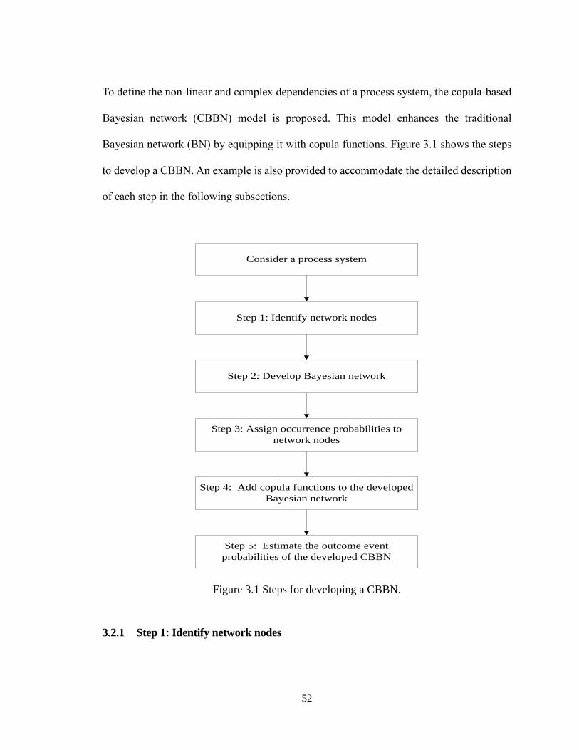
52
To define the non-linear and complex dependencies of a process system, the copula-based
Bayesian network (CBBN) model is proposed. This model enhances the traditional
Bayesian network (BN) by equipping it with copula functions. Figure 3.1 shows the steps
to develop a CBBN. An example is also provided to accommodate the detailed description
of each step in the following subsections.
Step 1: Identify network nodes
Step 2: Develop Bayesian network
Step 3: Assign occurrence probabilities to
network nodes
Step 4: Add copula functions to the developed
Bayesian network
Consider a process system
Step 5: Estimate the outcome event
probabilities of the developed CBBN
Figure 3.1 Steps for developing a CBBN.
3.2.1 Step 1: Identify network nodes
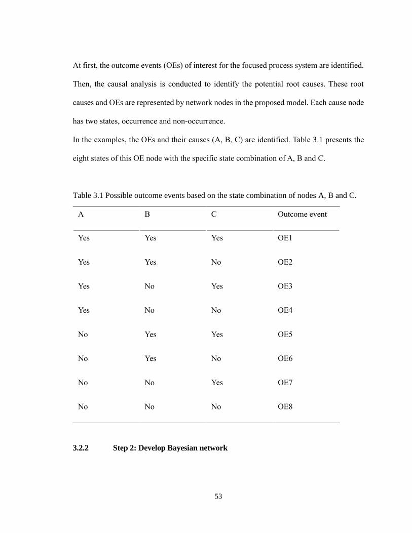
53
At first, the outcome events (OEs) of interest for the focused process system are identified.
Then, the causal analysis is conducted to identify the potential root causes. These root
causes and OEs are represented by network nodes in the proposed model. Each cause node
has two states, occurrence and non-occurrence.
In the examples, the OEs and their causes (A, B, C) are identified. Table 3.1 presents the
eight states of this OE node with the specific state combination of A, B and C.
Table 3.1 Possible outcome events based on the state combination of nodes A, B and C.
A B C Outcome event
Yes Yes Yes OE1
Yes Yes No OE2
Yes No Yes OE3
Yes No No OE4
No Yes Yes OE5
No Yes No OE6
No No Yes OE7
No No No OE8
3.2.2 Step 2: Develop Bayesian network
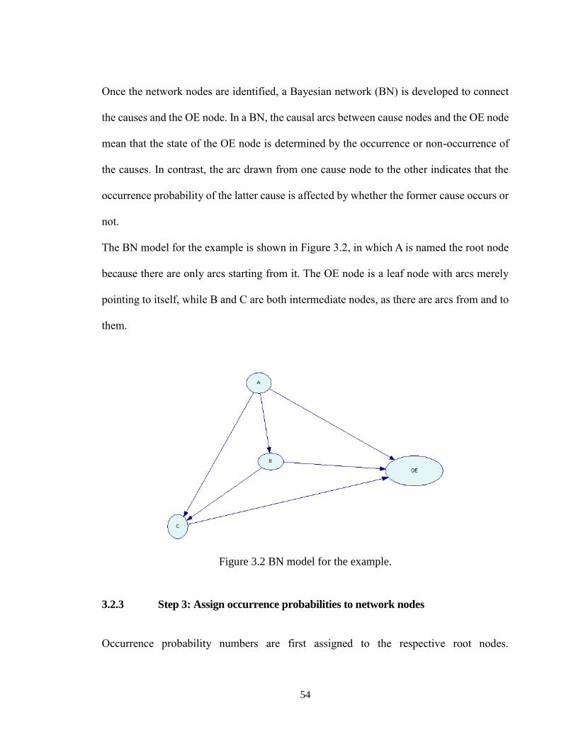
54
Once the network nodes are identified, a Bayesian network (BN) is developed to connect
the causes and the OE node. In a BN, the causal arcs between cause nodes and the OE node
mean that the state of the OE node is determined by the occurrence or non-occurrence of
the causes. In contrast, the arc drawn from one cause node to the other indicates that the
occurrence probability of the latter cause is affected by whether the former cause occurs or
not.
The BN model for the example is shown in Figure 3.2, in which A is named the root node
because there are only arcs starting from it. The OE node is a leaf node with arcs merely
pointing to itself, while B and C are both intermediate nodes, as there are arcs from and to
them.
Figure 3.2 BN model for the example.
3.2.3 Step 3: Assign occurrence probabilities to network nodes
Occurrence probability numbers are first assigned to the respective root nodes.
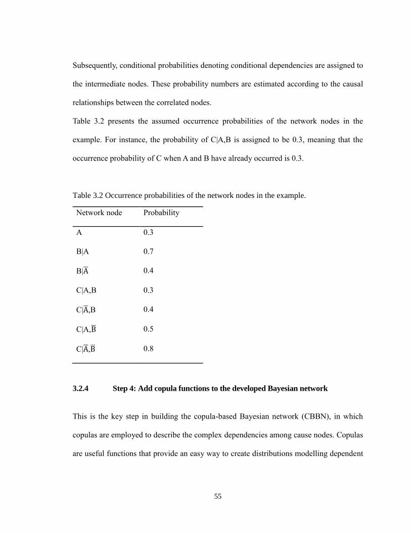
55
Subsequently, conditional probabilities denoting conditional dependencies are assigned to
the intermediate nodes. These probability numbers are estimated according to the causal
relationships between the correlated nodes.
Table 3.2 presents the assumed occurrence probabilities of the network nodes in the
example. For instance, the probability of C|A,B is assigned to be 0.3, meaning that the
occurrence probability of C when A and B have already occurred is 0.3.
Table 3.2 Occurrence probabilities of the network nodes in the example.
Network node Probability
A 0.3
B|A 0.7
B|A̅ 0.4
C|A,B 0.3
C|A̅,B 0.4
C|A,B̅ 0.5
C|A̅,B̅ 0.8
3.2.4 Step 4: Add copula functions to the developed Bayesian network
This is the key step in building the copula-based Bayesian network (CBBN), in which
copulas are employed to describe the complex dependencies among cause nodes. Copulas
are useful functions that provide an easy way to create distributions modelling dependent
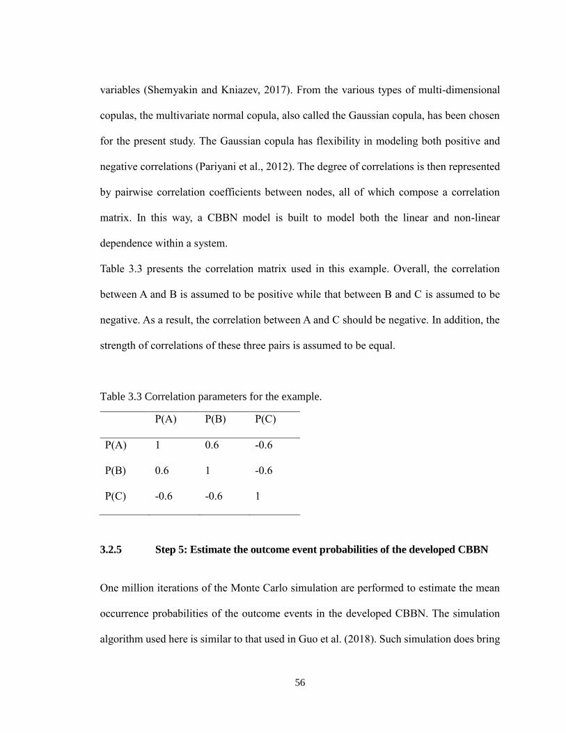
56
variables (Shemyakin and Kniazev, 2017). From the various types of multi-dimensional
copulas, the multivariate normal copula, also called the Gaussian copula, has been chosen
for the present study. The Gaussian copula has flexibility in modeling both positive and
negative correlations (Pariyani et al., 2012). The degree of correlations is then represented
by pairwise correlation coefficients between nodes, all of which compose a correlation
matrix. In this way, a CBBN model is built to model both the linear and non-linear
dependence within a system.
Table 3.3 presents the correlation matrix used in this example. Overall, the correlation
between A and B is assumed to be positive while that between B and C is assumed to be
negative. As a result, the correlation between A and C should be negative. In addition, the
strength of correlations of these three pairs is assumed to be equal.
Table 3.3 Correlation parameters for the example.
P(A) P(B) P(C)
P(A) 1 0.6 -0.6
P(B) 0.6 1 -0.6
P(C) -0.6 -0.6 1
3.2.5 Step 5: Estimate the outcome event probabilities of the developed CBBN
One million iterations of the Monte Carlo simulation are performed to estimate the mean
occurrence probabilities of the outcome events in the developed CBBN. The simulation
algorithm used here is similar to that used in Guo et al. (2018). Such simulation does bring
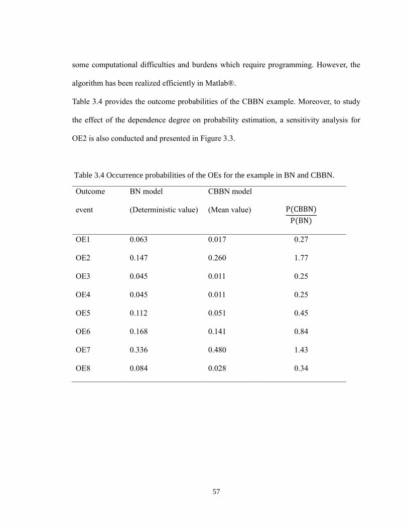
57
some computational difficulties and burdens which require programming. However, the
algorithm has been realized efficiently in Matlab®.
Table 3.4 provides the outcome probabilities of the CBBN example. Moreover, to study
the effect of the dependence degree on probability estimation, a sensitivity analysis for
OE2 is also conducted and presented in Figure 3.3.
Table 3.4 Occurrence probabilities of the OEs for the example in BN and CBBN.
Outcome
event
BN model
(Deterministic value)
CBBN model
(Mean value)
P(CBBN)
P(BN)
OE1 0.063 0.017 0.27
OE2 0.147 0.260 1.77
OE3 0.045 0.011 0.25
OE4 0.045 0.011 0.25
OE5 0.112 0.051 0.45
OE6 0.168 0.141 0.84
OE7 0.336 0.480 1.43
OE8 0.084 0.028 0.34
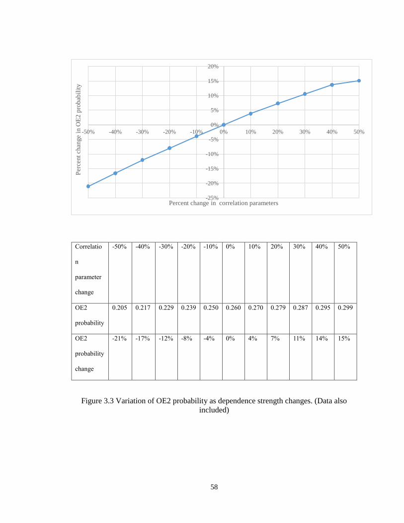
58
Correlatio
n
parameter
change
-50% -40% -30% -20% -10% 0% 10% 20% 30% 40% 50%
OE2
probability
0.205 0.217 0.229 0.239 0.250 0.260 0.270 0.279 0.287 0.295 0.299
OE2
probability
change
-21% -17% -12% -8% -4% 0% 4% 7% 11% 14% 15%
Figure 3.3 Variation of OE2 probability as dependence strength changes. (Data also
included)
-25%
-20%
-15%
-10%
-5%
0%
5%
10%
15%
20%
-50% -40% -30% -20% -10% 0% 10% 20% 30% 40% 50%
Per
cent
chan
ge
in O
E2
pro
bab
ilit
y
Percent change in correlation parameters
59
3.2.6 Comparison: Estimate the outcome event probabilities of the developed
BN
To distinguish the proposed CBBN model from the traditional BN model, the deterministic
probabilities of the outcome events in the BN are also estimated.
Taking OE7, for example, without considering copulas, the deterministic probability is
simply as follows.
P(OE7)=P( A̅ )P( B̅ | A̅ )P(C| A̅ , B̅ )=[1- P(A)][1-P(B| A̅ )]P(C| A̅ , B̅ )=(1-0.3)(1-0.4)0.8=0.336
(3.1)
Similarly, other outcome event probabilities have been derived and summarized in Table
3.4.
3.2.7 Discussion of the results for the example
Table 3.4 shows that the probabilities of OE2 and OE 7 in CBBN are larger than those in
BN. Conversely, other outcome event probabilities in CBBN are smaller than those in BN.
These are caused by the effect of the copula. As Table 3.3 shows, nodes A and B are
positively correlated, nodes A and C are negatively correlated, and nodes B and C are
negatively correlated. Thus, when A occurs, B also tends to occur. Subsequently, C tends
to not occur, leading to the increased probability of OE2. In contrast, when neither A nor B
occurs, C is more likely to occur, which increases OE7 probability.
As can be seen in Figure 3.3, OE2 probability rises steadily as the dependence grows
stronger. When there is a small increase or decrease in correlation parameters (ρ), the
absolute change in OE2 probability is almost identical. For instance, a +20% or -20%
60
change in correlation parameters only results in about a +7% or -8% change, respectively,
in estimated OE2 probability, which are very close. Nevertheless, as the percentage change
of correlation parameters becomes larger, the probability of OE2 decreases faster than it
increases. Figure 3.3 shows that OE2 probability falls by 21%, compared to its increase of
only 15% when the deviation in strength of dependence is 50%. Specifically, a -50% fall
in correlation parameters (i.e., |ρ|=0.3) decreases OE2 probability to 0.205, approaching its
value calculated in the case of the BN model (0.147). In contrast, a +50% rise in correlation
parameters (i.e., |ρ|=0.9) increases OE2 probability to 0.299, near the probability of node
A (0.3). This phenomenon was illustrated in Guo et al. (2018), which argued that for AND
logic, the probability of an outcome tends to approach the minimal probabilities of its
causation factors when there is high dependence among them. As a result, the maximal
increased OE2 probability can only reach 0.3, showing that the limit of increase in the
probability of OE2 is smaller than that of decrease.
To conclude this sensitivity analysis, the percent change in OE2 probability is symmetrical
when the percent change in correlation parameters is relatively small but then becomes
asymmetrical when the extent of change in correlation parameters is larger.
Application of the copula-based Bayesian network
To validate the proposed CBBN model for modeling complex dependencies in risk analysis,
a practical case report issued by the U.S. Chemical Safety and Hazard Identification Board
is examined. As can be found in the incident report, the June 13, 2013 reboiler rupture,
explosion and fire at the Williams Geismar Olefins Plant caused 2 fatalities and 167 injuries
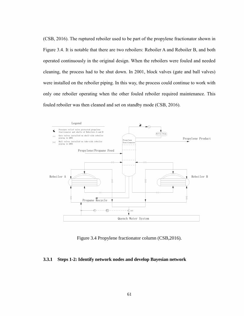
61
(CSB, 2016). The ruptured reboiler used to be part of the propylene fractionator shown in
Figure 3.4. It is notable that there are two reboilers: Reboiler A and Reboiler B, and both
operated continuously in the original design. When the reboilers were fouled and needed
cleaning, the process had to be shut down. In 2001, block valves (gate and ball valves)
were installed on the reboiler piping. In this way, the process could continue to work with
only one reboiler operating when the other fouled reboiler required maintenance. This
fouled reboiler was then cleaned and set on standby mode (CSB, 2016).
Reboiler A Reboiler B
Quench Water System
Propane Recycle
Propylene/Propane Feed
PropyleneFractionator
Propylene Product
Reflux Drum
PCPT FCV
Pressure relief valve protected propylenefractionator and shells of Reboilers A and B
Gate valves installed on shell-side reboilerpiping in 2001
Ball valves installed on tube-side reboilerpiping in 2001
Legend
Figure 3.4 Propylene fractionator column (CSB,2016).
3.3.1 Steps 1-2: Identify network nodes and develop Bayesian network
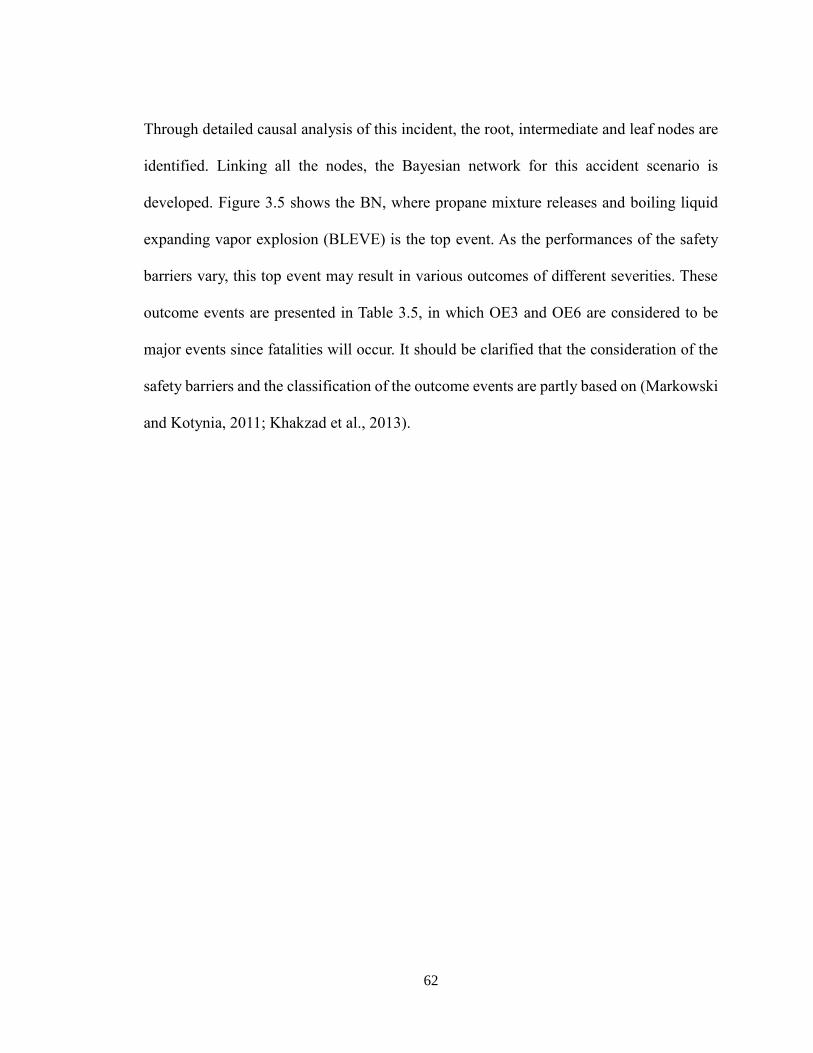
62
Through detailed causal analysis of this incident, the root, intermediate and leaf nodes are
identified. Linking all the nodes, the Bayesian network for this accident scenario is
developed. Figure 3.5 shows the BN, where propane mixture releases and boiling liquid
expanding vapor explosion (BLEVE) is the top event. As the performances of the safety
barriers vary, this top event may result in various outcomes of different severities. These
outcome events are presented in Table 3.5, in which OE3 and OE6 are considered to be
major events since fatalities will occur. It should be clarified that the consideration of the
safety barriers and the classification of the outcome events are partly based on (Markowski
and Kotynia, 2011; Khakzad et al., 2013).
63
Figure 3.5 Bayesian network for propane release from Reboiler B.
Table 3.5 Outcome event nodes depending on the performance of safety nodes.
Immediate
ignition barrier
Late ignition
barrier
Sprinkler Alarm Outcome event
work work - - Dispersion (OE1)
work fail work - Dispersion (OE1)
work fail fail work
Vapor cloud explosion (VCE)/Flash
fire (FF) (OE2)
work fail fail fail VCE/FF and fatalities (OE3)
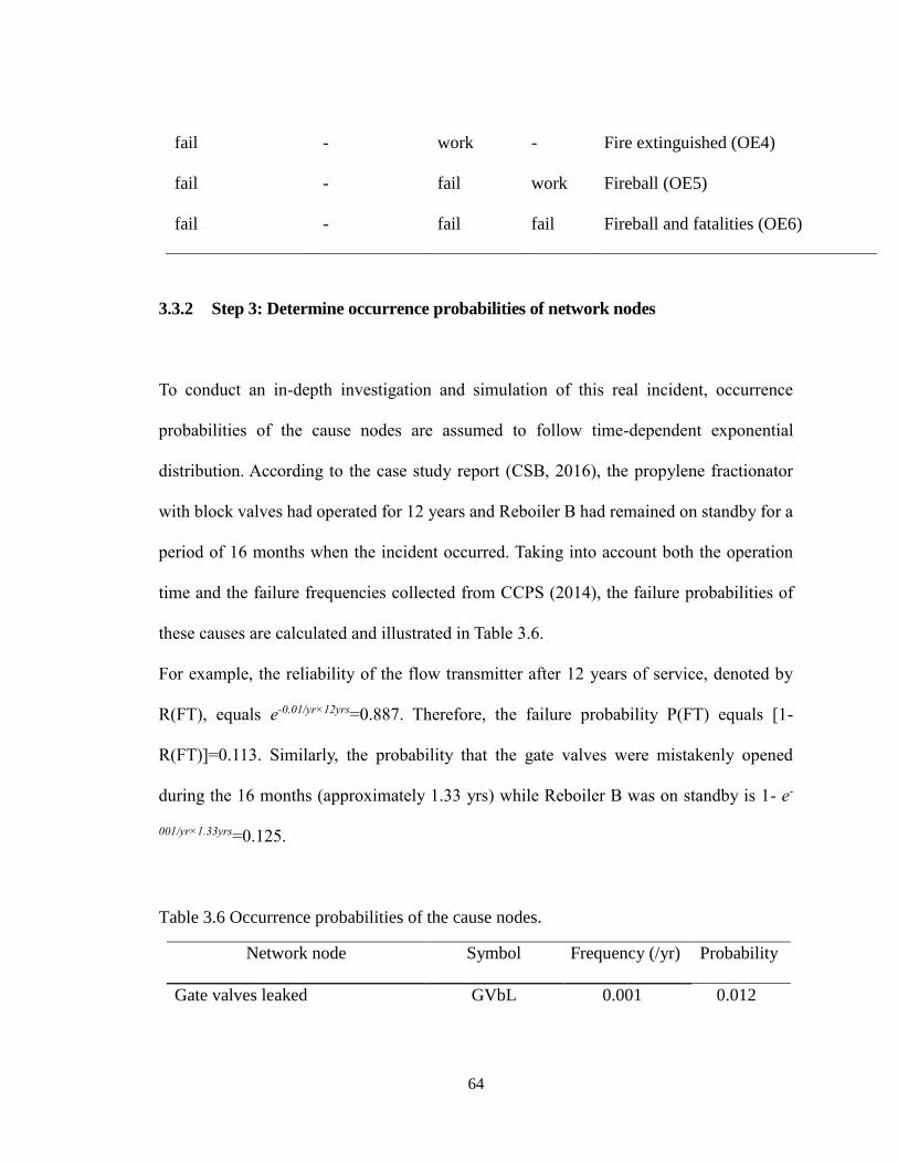
64
fail - work - Fire extinguished (OE4)
fail - fail work Fireball (OE5)
fail - fail fail Fireball and fatalities (OE6)
3.3.2 Step 3: Determine occurrence probabilities of network nodes
To conduct an in-depth investigation and simulation of this real incident, occurrence
probabilities of the cause nodes are assumed to follow time-dependent exponential
distribution. According to the case study report (CSB, 2016), the propylene fractionator
with block valves had operated for 12 years and Reboiler B had remained on standby for a
period of 16 months when the incident occurred. Taking into account both the operation
time and the failure frequencies collected from CCPS (2014), the failure probabilities of
these causes are calculated and illustrated in Table 3.6.
For example, the reliability of the flow transmitter after 12 years of service, denoted by
R(FT), equals e-0.01/yr×12yrs=0.887. Therefore, the failure probability P(FT) equals [1-
R(FT)]=0.113. Similarly, the probability that the gate valves were mistakenly opened
during the 16 months (approximately 1.33 yrs) while Reboiler B was on standby is 1- e-
001/yr×1.33yrs=0.125.
Table 3.6 Occurrence probabilities of the cause nodes.
Network node Symbol Frequency (/yr) Probability
Gate valves leaked GVbL 0.001 0.012
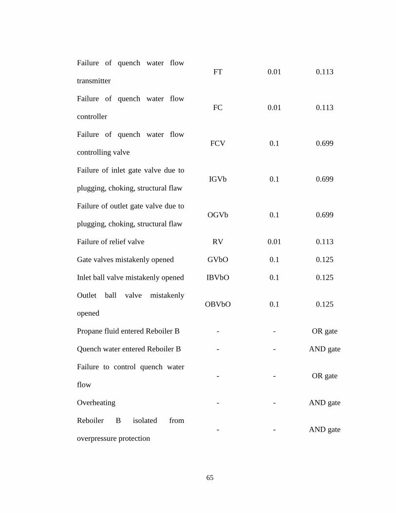
65
Failure of quench water flow
transmitter
FT 0.01 0.113
Failure of quench water flow
controller
FC 0.01 0.113
Failure of quench water flow
controlling valve
FCV 0.1 0.699
Failure of inlet gate valve due to
plugging, choking, structural flaw
IGVb 0.1 0.699
Failure of outlet gate valve due to
plugging, choking, structural flaw
OGVb 0.1 0.699
Failure of relief valve RV 0.01 0.113
Gate valves mistakenly opened GVbO 0.1 0.125
Inlet ball valve mistakenly opened IBVbO 0.1 0.125
Outlet ball valve mistakenly
opened
OBVbO 0.1 0.125
Propane fluid entered Reboiler B - - OR gate
Quench water entered Reboiler B - - AND gate
Failure to control quench water
flow
- - OR gate
Overheating - - AND gate
Reboiler B isolated from
overpressure protection
- - AND gate
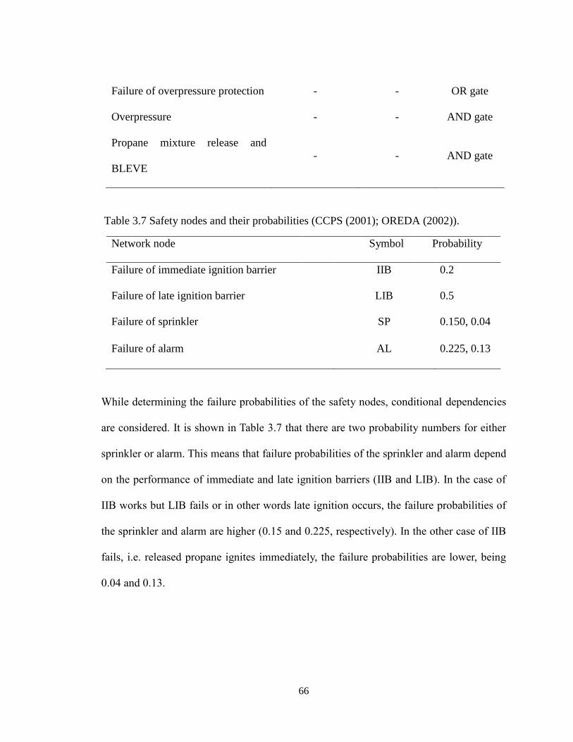
66
Failure of overpressure protection - - OR gate
Overpressure - - AND gate
Propane mixture release and
BLEVE
- - AND gate
Table 3.7 Safety nodes and their probabilities (CCPS (2001); OREDA (2002)).
Network node Symbol Probability
Failure of immediate ignition barrier IIB 0.2
Failure of late ignition barrier LIB 0.5
Failure of sprinkler SP 0.150, 0.04
Failure of alarm AL 0.225, 0.13
While determining the failure probabilities of the safety nodes, conditional dependencies
are considered. It is shown in Table 3.7 that there are two probability numbers for either
sprinkler or alarm. This means that failure probabilities of the sprinkler and alarm depend
on the performance of immediate and late ignition barriers (IIB and LIB). In the case of
IIB works but LIB fails or in other words late ignition occurs, the failure probabilities of
the sprinkler and alarm are higher (0.15 and 0.225, respectively). In the other case of IIB
fails, i.e. released propane ignites immediately, the failure probabilities are lower, being
0.04 and 0.13.
67
3.3.3 Step 4: Integrate copula functions to the developed Bayesian network
After analyzing the possible interrelationships of the network nodes, reasonable correlation
matrices are designed and shown in Tables 3.8-.3.11. As Table 3.8 shows, the correlation
parameter (ρ) between the causes that let quench water enter Reboiler B is assumed as 0.8,
which means there is very significant dependence. This is because it is likely that both the
inlet ball valve (IBVbO) and the outlet ball valve (OBVbO) of Reboiler B were mistakenly
opened. For a similar reason, the failures of the inlet gate valve (IGVb) and the outlet gate
valve (OGVb) probability occur simultaneously, justifying the assumption that the ρ
between these two should be 0.7, indicating significant dependence, as shown in Table 3.10.
Table 3.9 shows that the failures of the flow transmitter (FT), flow controller (FC) a d flow
controlling valve (FCV) are moderately dependent (i.e. ρ=0.6) since these components
make up the quench water control system and therefore work under the same environment.
Table 3.11 presents the dependence strengths among the safety nodes represented by
pairwise correlation parameters. On average, it is assumed that the dependence between a
safety node and its closer neighboring node is more significant due to potentially stronger
interactions.
The Gaussian copulas with these correlation parameters are then added to the existing BN,
building the CBBN, where both linear and non-linear dependence of the network nodes are
considered.
Table 3.8 Correlation parameters between the causes of quench water entering Reboiler
B.
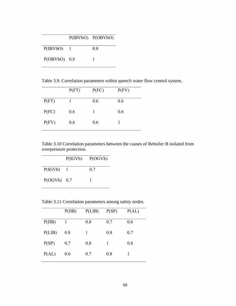
68
P(IBVbO) P(OBVbO)
P(IBVbO) 1 0.8
P(OBVbO) 0.8 1
Table 3.9. Correlation parameters within quench water flow control system.
P(FT) P(FC) P(FV)
P(FT) 1 0.6 0.6
P(FC) 0.6 1 0.6
P(FV) 0.6 0.6 1
Table 3.10 Correlation parameters between the causes of Reboiler B isolated from
overpressure protection.
P(IGVb) P(OGVb)
P(IGVb) 1 0.7
P(OGVb) 0.7 1
Table 3.11 Correlation parameters among safety nodes.
P(IIB) P(LIB) P(SP) P(AL)
P(IIB) 1 0.8 0.7 0.6
P(LIB) 0.8 1 0.8 0.7
P(SP) 0.7 0.8 1 0.8
P(AL) 0.6 0.7 0.8 1
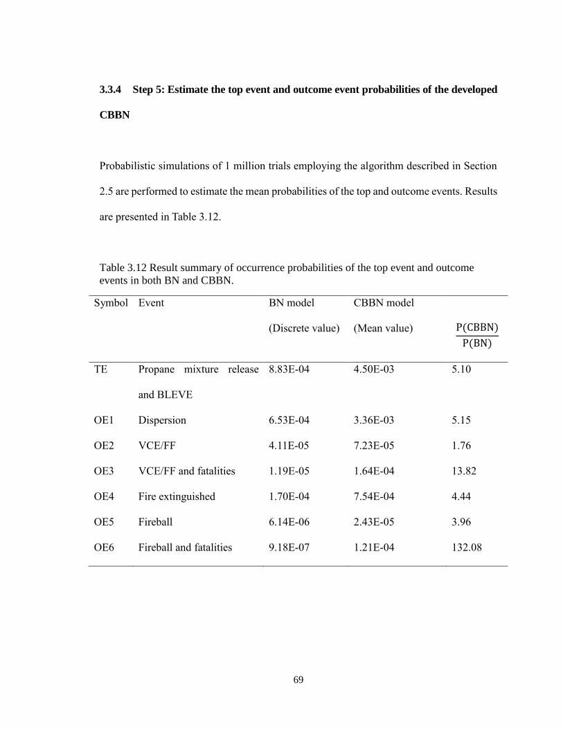
69
3.3.4 Step 5: Estimate the top event and outcome event probabilities of the developed
CBBN
Probabilistic simulations of 1 million trials employing the algorithm described in Section
2.5 are performed to estimate the mean probabilities of the top and outcome events. Results
are presented in Table 3.12.
Table 3.12 Result summary of occurrence probabilities of the top event and outcome
events in both BN and CBBN.
Symbol Event BN model
(Discrete value)
CBBN model
(Mean value)
P(CBBN)
P(BN)
TE Propane mixture release
and BLEVE
8.83E-04 4.50E-03 5.10
OE1 Dispersion 6.53E-04 3.36E-03 5.15
OE2 VCE/FF 4.11E-05 7.23E-05 1.76
OE3 VCE/FF and fatalities 1.19E-05 1.64E-04 13.82
OE4 Fire extinguished 1.70E-04 7.54E-04 4.44
OE5 Fireball 6.14E-06 2.43E-05 3.96
OE6 Fireball and fatalities 9.18E-07 1.21E-04 132.08
70
3.3.5 Comparison: Estimate the top event and outcome event probabilities of the
developed BN
As a comparison, the developed Bayesian network model, which only captures linear
dependence, is also studied. The probabilities of the top event and OE6 are calculated as
shown below:
P(TE)=(GVbL+GVbO-GVbL×GVbO)IBVbO×OBVbO(FT+FC+FCV-FT×FC-FC×FCV-
FT×FCV+FT×FC×FCV)(IGVb×OGVb+RV-IGVb×OGVb×RV) (3.2)
P(OE6)=P(TE)P(IIB)P(SP|IIB)P(AL|IIB) (3.3)
Where GVbL, GVbO,…, P(AL|IIB) represent the respective probabilities in Tables 3.6 and
3.7. Similarly, the probabilities of other outcome events are derived and presented in Table
3.12.
Discussion
3.4.1 The top event probability in CBBN and BN
Table 3.12 shows that the probability of the top event in CBBN is significantly larger than
that in BN, which can be explained by the effect of non-linear dependencies of the root
nodes as defined by Tables 3.8-3.10. Root nodes IBVbO and OBVbO are positively
correlated under the AND gate and so are the nodes IGVb and OGVb. This correlation
leads to the increased probabilities of the respective intermediate nodes, which tend to
approach 0.125 and 0.699, almost 8 and 1.43 times as large as the BN case. This increase
71
finally contributes to the increased top event probability. There is an OR gate connecting
the dependent root nodes FT, FC and FV, causing the decreased probability of the
intermediate node Failure to control quench water flow. However, this probability only
drops from 0.763 to nearly 0.699. Such an increase for the AND gate as well as a decrease
for the OR gate in intermediate node probabilities are explained in (Guo et al., 2018). As
Eq. (3.2) shows, compared to the significant increased probabilities resulting from the
dependence within AND gates, this decrease does not have a large effect on the top event
probability. As a result, the probability of propane release and BLEVE is 5.10 times as
large in CBBN as in BN.
3.4.2 The outcome event probabilities in CBBN and BN
Table 3.12 shows that the probabilities of all the outcome events are also obviously greater
in CBBN than in BN. In the BN for this scenario, only the conditional dependence of the
performances of the sprinkler and alarm on the performance of the immediate ignition
barrier are defined by Table 3.7. While in CBBN, non-linear dependence is also
incorporated by correlation parameters as presented in Tables 3.8-3.11. The increased top
event probability as explained in Section 4.1 accounts for the increase of all the outcome
event probabilities. In particular, the probabilities of OE3 and OE6, where fatalities occur,
increase most sharply. This is because the positive non-linear dependence among the safety
nodes increases the occurrence probability that most or all safety barriers fail at the same
time, which results in OE3 or OE6. Quantitatively speaking, similar to the demonstration
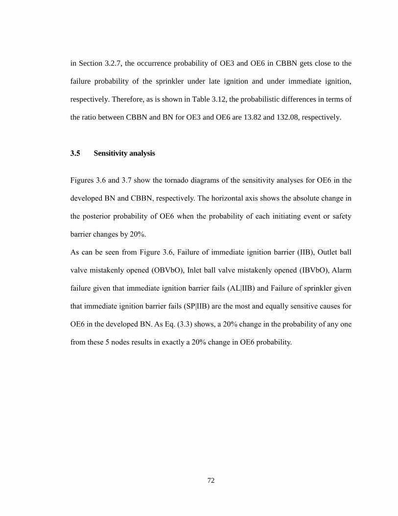
72
in Section 3.2.7, the occurrence probability of OE3 and OE6 in CBBN gets close to the
failure probability of the sprinkler under late ignition and under immediate ignition,
respectively. Therefore, as is shown in Table 3.12, the probabilistic differences in terms of
the ratio between CBBN and BN for OE3 and OE6 are 13.82 and 132.08, respectively.
Sensitivity analysis
Figures 3.6 and 3.7 show the tornado diagrams of the sensitivity analyses for OE6 in the
developed BN and CBBN, respectively. The horizontal axis shows the absolute change in
the posterior probability of OE6 when the probability of each initiating event or safety
barrier changes by 20%.
As can be seen from Figure 3.6, Failure of immediate ignition barrier (IIB), Outlet ball
valve mistakenly opened (OBVbO), Inlet ball valve mistakenly opened (IBVbO), Alarm
failure given that immediate ignition barrier fails (AL|IIB) and Failure of sprinkler given
that immediate ignition barrier fails (SP|IIB) are the most and equally sensitive causes for
OE6 in the developed BN. As Eq. (3.3) shows, a 20% change in the probability of any one
from these 5 nodes results in exactly a 20% change in OE6 probability.
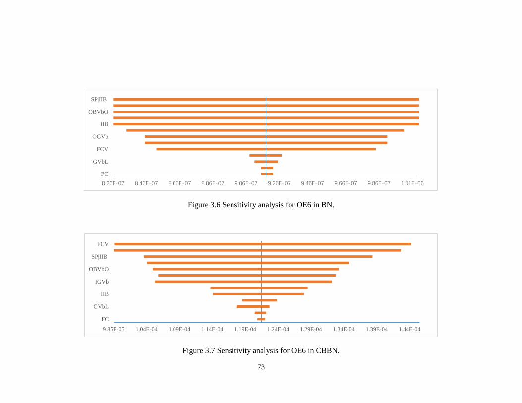
73
Figure 3.6 Sensitivity analysis for OE6 in BN.
Figure 3.7 Sensitivity analysis for OE6 in CBBN.
8.26E-07 8.46E-07 8.66E-07 8.86E-07 9.06E-07 9.26E-07 9.46E-07 9.66E-07 9.86E-07 1.01E-06
FC
GVbL
FCV
OGVb
IIB
OBVbO
SP|IIB
9.85E-05 1.04E-04 1.09E-04 1.14E-04 1.19E-04 1.24E-04 1.29E-04 1.34E-04 1.39E-04 1.44E-04
FC
GVbL
IIB
IGVb
OBVbO
SP|IIB
FCV
74
In contrast, Figure 3.7 shows that Failure of quench water flow controlling valve (FCV) is
the most sensitive cause for OE6 in the developed CBBN. This is due to the effect of
dependence on the OR gate: the probability of the intermediate node tends to approach the
maximal root node probability when there is dependence among root nodes. In this case,
FCV accounts for the largest failure probability leading to the intermediate node Failure to
control quench water flow. Consequently, FCV is dominant in determining the probability
of this intermediate node and thus significantly affects the top event and then OE6
probability. Gate valves mistakenly opened (GVbO) is shown to be the second most
sensitive parameter because its probability is much larger than the Gate valves leaked
(GVbL) probability.
Figure 3.7 also shows that OE6 is thirdly sensitive to SP|IIB. The reason is concerned with
the AND logic of an event tree, which means that OE6 probability depends more on the
safety nodes with smaller probabilities. Therefore, the impact of AL|IIB and IIB becomes
less significant in comparison with the case of BN. In addition, it is clear that IBVbO and
OBVbO both rank as the 4th sensitive parameters. This is because of the effect of
dependence on the AND gate: the intermediate node probability will get closer to the
minimal root node probability when the dependence is considered. Returning to this
example, the initial probability of Quench water entering Reboiler B is close to 0.699, the
probability value of both IBVbO and OBVbO. When the probability value of IBVbO
decreases by 20%, for instance, the intermediate node probability will get closer to this
decreased probability number of IBVbO, resulting in a sharp decrease in OE6 probability.
In contrast, the probability of OE6 does not change as considerably as the former analysis
75
for decrease when there is a 20% increase in IBVbO probability, because the intermediate
node probability still tends to approach 0.699, which is the probability of OBVbO as the
minimal probability.
Probability updating
Probability updating is usually performed to find the most probable causes of a specific
outcome event (Abimbola et al., 2015). Abimbola et al. (2015) and Khakzad et al. (2013)
have conducted exhaustive updating of node probabilities in a Bayesian network based on
Bayes theorem. In this paper, the updating analysis is performed by GeNIe 2.1
(https://www.bayesfusion.com/genie/).
According to the accident report (CSB, 2016), a rupture in Reboiler B caused BLEVE and
a large amount of propane mixture release, which ignited, resulting in a fireball and two
fatalities. Therefore, the state of node Outcome event is instantiated to OE6. Figure 3.8
shows the posterior probabilities of the other nodes based on this evidence. The most
probable causes of OE6 are determined to be as follows. The gate valves were mistakenly
opened, letting propane fluid enter Reboiler B. Quench water entered Reboiler B by
mistakenly opened ball valves and the failure of the quench water flow controlling system
due to the failure of the flow controlling valve, introducing heat to Reboiler B. The propane
mixture was continuously heated, leading to overpressure. Unfortunately, the gate valves
failed, isolating Reboiler B from the overpressure protection system. Reboiler B finally
ruptured, causing BLEVE and then a fireball, killing two workers nearby, because of the
failure of the immediate ignition barrier, sprinkler and alarm. This diagnostic analysis
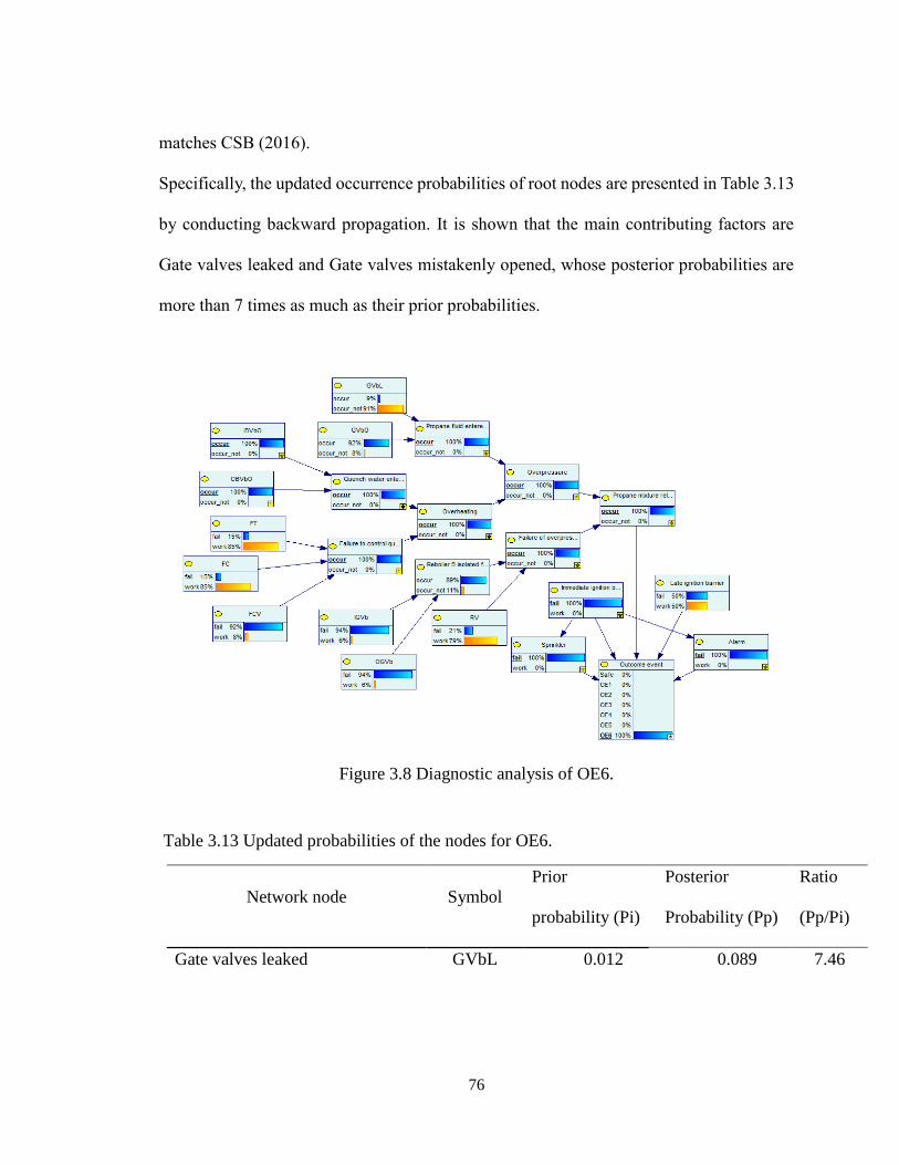
76
matches CSB (2016).
Specifically, the updated occurrence probabilities of root nodes are presented in Table 3.13
by conducting backward propagation. It is shown that the main contributing factors are
Gate valves leaked and Gate valves mistakenly opened, whose posterior probabilities are
more than 7 times as much as their prior probabilities.
Figure 3.8 Diagnostic analysis of OE6.
Table 3.13 Updated probabilities of the nodes for OE6.
Network node Symbol
Prior
probability (Pi)
Posterior
Probability (Pp)
Ratio
(Pp/Pi)
Gate valves leaked GVbL 0.012 0.089 7.46
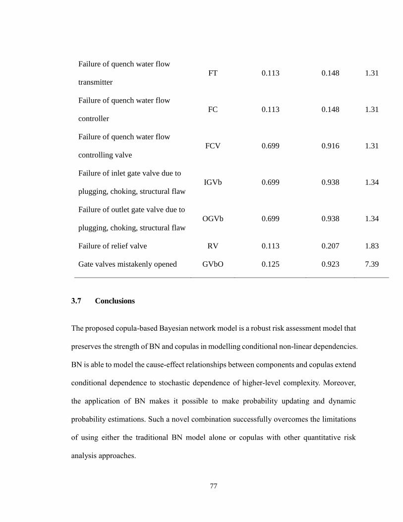
77
Failure of quench water flow
transmitter
FT 0.113 0.148 1.31
Failure of quench water flow
controller
FC 0.113 0.148 1.31
Failure of quench water flow
controlling valve
FCV 0.699 0.916 1.31
Failure of inlet gate valve due to
plugging, choking, structural flaw
IGVb 0.699 0.938 1.34
Failure of outlet gate valve due to
plugging, choking, structural flaw
OGVb 0.699 0.938 1.34
Failure of relief valve RV 0.113 0.207 1.83
Gate valves mistakenly opened GVbO 0.125 0.923 7.39
Conclusions
The proposed copula-based Bayesian network model is a robust risk assessment model that
preserves the strength of BN and copulas in modelling conditional non-linear dependencies.
BN is able to model the cause-effect relationships between components and copulas extend
conditional dependence to stochastic dependence of higher-level complexity. Moreover,
the application of BN makes it possible to make probability updating and dynamic
probability estimations. Such a novel combination successfully overcomes the limitations
of using either the traditional BN model alone or copulas with other quantitative risk
analysis approaches.
78
The proposed model is tested on a real case study. The results of the proposed model are
compared with the results of a traditional BN. It is observed that the non-linear dependence
modeled by copulas yields significant increases in outcome probabilities, which are closer
to reality. This highlights the significance of dependence among causes on the occurrence
of undesired events. Moreover, this case study proves that the CBBN model is innovative
and scientifically viable to be implemented to industry.
The proposed revised model illustrates the use of copulas in a very simple and easy to
implement way. It captures the inherently complex dependencies of process variables, e.g.,
common failure modes. Sensitivity analysis presents the crucial factors that affect the
accident scenario. A diagnostic analysis is also performed, showing the most likely the
causes of the BLEVE and propane release. Results confirm the effectiveness of this model.
Results confirm the advantage of this model against other similar approaches.
The proposed model needs further tests to ensure its wider applicability. This work can also
be improved by considering advanced algorithms for data processing and estimating
correlation parameters.
References
Abimbola, M., Khan, F., Khakzad, N., Butt, S., 2015. Safety and risk analysis of
managed pressure drilling operation using Bayesian network. Safety Science 76, 133-
144.
Ale, B., van Gulijk, C., Hanea, A., Hanea, D., Hudson, P., Lin, P., Sillem, S., 2014.
Towards BBN based risk modelling of process plants. Saf. Sci. 69, 48-56.
79
Aqlan, F., Mustafa Ali, E., 2014. Integrating lean principles and fuzzy bow-tie analysis
for risk assessment in chemical industry. Journal of Loss Prevention in the Process
Industries 29, 39-48.
CCPS, 2014. Guidelines for Initiating Events and Independent Protection Layers in Layer
of Protection Analysis.
CCPS, 2003. Guidelines for Chemical Process Quantitative Risk Analysis (2nd Edition).
Center for Chemical Process Safety/AIChE.
CCPS, 2001. Layer of Protection Analysis - Simplified Process Risk Assessment. Center
for Chemical Process Safety/AIChE.
CSB, 2016. Williams olefins plant explosion and fire. Investigation No. 2013-03-I-
LA. https://www.csb.gov/williams-olefins-plant-explosion-and-fire-/ (last checked on
11.08.18).
De Dianous, V., Fievez, C., 2006. ARAMIS project: A more explicit demonstration of
risk control through the use of bow-tie diagrams and the evaluation of safety barrier
performance. J. Hazard. Mater. 130, 220-233.
Guo, C., Khan, F., Imtiaz, S., 2018. Risk assessment of process system considering
dependencies. J Loss Prev Process Ind 55, 204-212.
80
Hashemi, S.J., Khan, F., Ahmed, S., 2016. Multivariate probabilistic safety analysis of
process facilities using the Copula Bayesian Network model. Computers and Chemical
Engineering 93, 128-142.
Khakzad, N., Khan, F., Amyotte, P., 2013. Dynamic safety analysis of process systems
by mapping bow-tie into Bayesian network. Process Safety and Environmental Protection
91, 46-53.
Lu, L., Liang, W., Zhang, L., Zhang, H., Lu, Z., Shan, J., 2015. A comprehensive risk
evaluation method for natural gas pipelines by combining a risk matrix with a bow-tie
model. Journal of Natural Gas Science and Engineering 25, 124-133.
Markowski, A.S., Kotynia, A., 2011. "Bow-tie" model in layer of protection analysis.
Process Saf. Environ. Prot. 89, 205-213.
Meel, A., Seider, W.D., 2006. Plant-specific dynamic failure assessment using Bayesian
theory. Chemical Engineering Science 61, 7036-7056.
Mohseni Ahooyi, T., Arbogast, J.E., Soroush, M., 2014. Applications of the rolling pin
method. 1. An efficient alternative to Bayesian network modeling and inference.
Industrial and Engineering Chemistry Research 54, 4316-4325.
Oktem, U.G., Seider, W.D., Soroush, M., Pariyani, A., 2013. Improve process safety with
near-miss analysis. Chem. Eng. Prog. 109, 20-27.
81
OREDA, 2002. OREDA : Offshore Reliability Data Handbook. OREDA Participants :
Distributed by Der Norske Veritas, Høvik, Norway.
Pariyani, A., Seider, W.D., Oktem, U.G., Soroush, M., 2012. Dynamic risk analysis using
alarm databases to improve process safety and product quality: Part II-Bayesian analysis.
AIChE J. 58, 826-841.
Pasman, H., Rogers, W., 2013. Bayesian networks make LOPA more effective, QRA
more transparent and flexible, and thus safety more definable! J Loss Prev Process Ind
26, 434-442.
Shemyakin, A., Kniazev, A., 2017. Introduction to Bayesian Estimation and Copula
Models of Dependence. John Wiley & Sons, Incorporated, Somerset.
Zilko, A.A., Kurowicka, D., Goverde, R.M.P., 2016. Modeling railway disruption lengths
with Copula Bayesian Networks. Transportation Research Part C: Emerging
Technologies 68, 350-368.
82
Chapter 4. Summary
Quantitative risk analysis (QRA) currently plays an important role in risk assessment and
safety management throughout the life cycle of process installations. To lower risks in the
earliest stage, QRA can be used in risk-based design, which focuses on inherent safety.
However, QRA is more often performed in the installation phase, which is after the
completion of the equipment layout and safety measures. In the Introduction and Overview
section of this thesis, a review of several popular QRA techniques and their strengths and
limitations is presented. As is explained, most existing QRA techniques, such as bow-tie,
do not take dependent failures into account. Although the Bayesian network incorporates
linear dependency into the risk analysis process, it cannot model non-linear dependency in
complex process systems.
To meet the need for the risk estimation of systems with complex dependencies, the thesis
proposes revisions of two traditional QRA methods by integrating copula functions. One
revised model is copula-based bow-tie (CBBT), which fits integrated systems where
dependency exists. The other is copula-based Bayesian network (CBBN), which is
considered more generally applicable than CBBT, since it captures both mutual and
stochastic dependencies by combining BN and copula functions.
4.1 Conclusions
Both models have been applied to practical cases that occur in chemical installation sites.
The causes and outcomes of accident scenarios are first identified. Monte Carlo simulations
83
are then employed while running these two copula-based models to count the mean
occurrence times of all the possible outcomes. These simulation results are compared with
the calculated deterministic probabilities from traditional bow-tie or Bayesian network
analysis. As is observed, the probabilities of severe outcome events, where all the safety
barriers fail to function, are considerably larger in copula-based models. This observation
shows the great influence of dependence among safety barriers on the occurrence of
accidents. It is also shown that the ignorance of potential dependency might result in an
underestimated risk. To reduce the risk caused by dependence effects, more independent
safety barriers are recommended to be integrated into process systems, if possible.
The proposed models demonstrate the use of copula in a simple and straightforward way.
The stochastic and non-linear dependencies among process variables, such as common
failure modes, are represented by means of copulas. Hence, these two copula-based models
can be employed as useful approaches when performing the risk assessment of complex
process systems with inherent dependencies. The specific conclusions for each model are
presented separately in the following subsections.
4.1.1 Development of copula-based bow-tie model
By integrating the stochastic dependencies among causes and bow-tie analysis, a copula-
based bow-tie model (CBBT) is developed. This revised model is first tested to study the
effect of dependence among initiating events on AND gates & OR gates. It has been proven
that positive dependence will increase the probability of an AND gate while decreasing the
probability of an OR gate. It also shows that as dependence is more significant, an AND
84
gate probability value becomes closer to the minimal initiating event probability. In
contrast, the probability value of an OR gate tends to approach the maximal probability
value of all the initiating events. These interesting findings highlight the importance of
monitoring potential dependent initiating events that may cause abnormal conditions so as
to prevent top events.
4.1.2 Development of copula-based Bayesian network model
This thesis proposes a copula-based Bayesian network model, which is a powerful tool for
modeling cause-effect relationships and conditional and stochastic dependencies. This
model is applied to a real-life case study about a disaster resulting from a reboiler rupture.
Causal analysis is performed and presented in the form of a Bayesian network. Simulation
results indicate that some dependent failures should be blamed for causing the BLEVE and
propane release, which match what occurred in reality. Sensitivity analysis identifies the
safety systems that need more inspection and maintenance.
4.2 Future work
The two models may be examined by a broader scope of contexts beyond chemical
processing industries to increase their applicability. Also, one of the limitations of the
present research is that when determining failure probabilities, expert opinions rather than
historical records are used. If sufficient on-site failure data become available, the proposed
methodologies will be more useful. Whether or not there are dependencies should first be
85
analyzed. Subsequently, if dependencies do exist, advanced algorithms for processing data
to estimate correlation parameters and model such dependencies should be further explored.
Last, the incorporation of accident precursors to allow dynamic updates of the estimated
probabilities in these copula-based models is an interesting subject for future research.