Copula-Dependent Default Risk in Intensity Models

Philipp J. Schonbucher and Dirk Schubert

Department of Statistics, Bonn University

November 2000, this version December 2001

Bonn University, Economics Faculty, Department of Statistics

Adenauerallee 24–42, 53113 Bonn, Germany,

Tel: +49-228-739264, Fax: +49-228-735050

email: P@Schonbucher.de

http://www.finasto.uni-bonn.de/schonbucher/

JEL Classification:G 13

Authors’ address: Department of Statistics, Faculty of Economics, Bonn University, Ad-

enauerallee 24–42, 53113 Bonn, Germany, Tel: +49-228-739264, Fax: +49-228-735050

email: P@Schonbucher.de, http://www.finasto.uni-bonn.de/˜schonbuc/

The authors would like to thank the Deutsche Forschungsgemeinschaft for financial sup-

port.

The authors thank Lutz Schlogl, Rudiger Frey, Ebbe Rogge and Kay Giesecke for helpful

discussions. Thanks for comments and suggestions go to the participants at the ’Work-

shop on Financial Mathematics’, McGill University, Montreal, the Risk Math Week 2001

in London and New York, the NYU Courant Institute Seminar on Mathematical Finance,

and the Eighth Annual CAP Workshop on Derivative Securities and Risk Management

at Columbia University.

Further comments and suggestions are welcome, all errors are our own.

Keywords: Default Risk, Intensity Models, Copula Functions

1

2

Copula-Dependent Default Risk in Intensity Models

In this paper we present a new approach to incorporate dynamic default

dependency in intensity-based default risk models. The model uses an

arbitrary default dependency structure which is specified by the Copula

of the times of default, this is combined with individual intensity-based

models for the defaults of the obligors without loss of the calibration

of the individual default-intensity models. The dynamics of the sur-

vival probabilities and credit spreads of individual obligors are derived

and it is shown that in situations with positive dependence, the default

of one obligor causes the credit spreads of the other obligors to jump

upwards, as it is experienced empirically in situations with credit con-

tagion. For the Clayton copula these jumps are proportional to the

pre-default intensity. If information about other obligors is excluded,

the model reduces to a standard intensity model for a single obligor,

thus greatly facilitating its calibration. To illustrate the results they

are also presented for Archimedean copulae in general, and Gumbel

and Clayton copulae in particular. Furthermore it is shown how the de-

fault correlation can be calibrated to a Gaussian dependency structure

of CreditMetrics-type.

JEL Classification: G13

3

1. Introduction

Recently there has been strong interest in the development of accurate models for default

dependencies. This interest is part of a general development towards an active and market-

based management of credit risks in banks and other financial institutions. It is recognized

that – unless the exposure is exceptionally large – individual defaults do not significantly

affect the risk of the portfolio as long as they can be diversified. If on the other hand

there are strong, systematic dependencies, even a portfolio containing a large number of

small loans can be highly risky.

In the drive to securitize and trade loan and bond portfolios, several new derivative se-

curities have been developed whose payoffs depend on the overall default behaviour of a

whole portfolio of underlying loans or bonds. Prominent examples are basket credit deriv-

atives and collateralised debt obligations (CDOs, CLOs, CBOs). These credit derivatives

are actively traded which requires a methodology to measure default- and market risks

on a day-by-day basis. A consistent model for default dependencies is essential to price

and hedge these structures.

Furthermore, with the increasing volume in credit derivatives transactions, counterparty

risk is recognized as a major source of risk which can affect the value of the credit protec-

tion bought. Here, too, a model for default dependencies is indispensable to assess and

manage these risks, and again this must be a dynamic model.

In this paper we provide a modelling framework for default dependency which differs in

several respects from other models in the literature. First, the model is a continuous-

time dynamic model, and defaults and default probabilities evolve consistently within

the model. In particular, the default probability of all obligors is continuously updated

according to the observed default / no default behaviour of the other obligors. Secondly,

the default dependency in the model can be specified in form of a copula of joint defaults at

a given time-horizon, i.e. essentially static information. Third, the model can be directly

calibrated to individual term structures of default intensities. Fourth, we allow for a much

more general specification of the dependency between default events than other models

in the literature. Furthermore, the analysis in this paper provides valuable insights in

the connection between default dependencies and the joint dynamics of default intensities

which are implicitly specified by specifying the default dependency. This information is

particularly valuable in risk management.

4

Most of the literature on default correlation is concerned with the credit risk of large port-

folios and based upon models like JPMorgan’s Credit Metrics (1997) or Credit Suisse’s

Credit Risk+ (1997), see Crouhy et.al. (2000) for a comparison. The Credit Metrics ap-

proach has been refined in the factor-based default risk models by Vasicek (1987), Belkin

et.al. (1998), Finger (1999) and Lucas et.al. (1999). These models also belong to the port-

folio credit risk models, but some analytical tractability is regained by assuming a certain

factor-dependence in the default mechanism. Here, the focus is the credit risk modelling

for portfolio-management and regulatory issues. Therefore, simplifying assumptions are

made on the individual default risk of the obligors, the dynamics of credit spreads and the

term structures of credit spreads. Default correlations are modelled more carefully, usu-

ally with a copula based upon a multivariate normal distribution. Because of the broad

focus on risk assessment, the models are generally not accurate and flexible enough to be

calibrated to the market and to be used for the pricing of traded structures. Nevertheless,

the data and the statistical analysis of default correlations on which these models are

based is useful.

A weak point of all portfolio-based approaches is that they do not adequately resolve the

dynamics of the value of the portfolio. For example, Credit Metrics is a one-period model

with two points in time and a very coarse attempt to capture some market risk through

rating changes. Credit Risk+ is set up in continuous-time but is only concerned with

default/survival (and not price changes) in the portfolio. So far, there has been no model

in the portfolio-based literature, which was able to consistently model default dependency

and market price risk in one continuous-time modelling framework, although the drive

towards securtisation and active management of credit risks as well as the rise in trading

of basket credit derivatives and CDOs requires precise such a model. One contribution of

this paper is to show how a consistent dynamic continuous-time model of defaults, default

dependency and changes in default risk can be constructed for any given form of default

dependency.

In order to point out the difficulties that may arise (and which have been largely ignored

so far), consider two obligors A and B whose defaults are highly correlated. We do not

know if or when they will default, but we have a joint distribution function F (tA, tB) of

the times of default τA of A and τB of B. The market prices of bonds issued by A will

reflect the default probability until maturity of the bond of A, and the market prices of

bonds issued by B the default probability of B. If obligor A defaults at some time t, a

fundamental change occurs in our probability assessment of the default likelihood of B:

While for t < τA, the default probability of B was the default probability until maturity

given that A will default some time after t, at τA it is the default probability given

5

that A defaults exactly now. As A and B are highly correlated, the second conditioning

information is much worse news on B’s chances of survival, and this discrete change in

information structure will cause a jump in the default probability of B at the time of

default of A, and vice versa. While there have been some attempts to frame Credit

Metrics into a continuous-time setup, these rational updating effects have been ignored so

far. In this paper we give a precise description at what times under which conditions the

presence of default dependence influences the dynamics of default intensities (and thus of

default probabilities).

In contrast to the portfolio models which can capture individual credit risk only very

coarsely, intensity-based single-name credit risk models provide a more flexible framework

to model the dynamics and the term structure of credit risk. Usually they are based upon

market variables such as credit spreads.

Most intensity models can be fitted easily to term structures of credit spreads and they

have effectively become market standard in the pricing of standard credit derivatives

such as credit default swaps. Important papers of this model class are Jarrow and Turn-

bull (1995) Duffie and Singleton (1999), Madan and Unal (1998), Lando (1998) and

Schonbucher (1999; 1998).

Two approaches have been followed to extend these intensity-based models to incorporate

default correlation and multiple defaults. The first, and simplest approach is to introduce

correlation in the dynamics of the default intensities of the obligors, but to keep the

models unchanged otherwise. This approach suffers from several disadvantages: The

default correlations that can be reached with this approach are typically too low when

compared with empirical default correlations, and furthermore it is very hard to derive

and analyze the resulting default dependency structure. The problem of low default

correlation becomes less severe when a large portfolio of different obligors is considered.

Therefore these models are used either enterprise-wide (e.g. CreditRisk+) or for large

CDOs (e.g. Duffie and Garleanu (1999)).

A refinement of this approach with more realistic default correlations is the infectious

defaults model by Davis and Lo (1999a; 1999b; 2000), further developed by Jarrow and Yu

(2000). There default intensities jointly jump upwards by a discrete amount at the onset

of a credit crisis. While intuitively very appealing, deriving the survival probability for a

single obligor is already a major task in this model which makes calibration very difficult.

Furthermore, the estimation of the jump factor of the default intensities is also nontrivial,

because it is not clear how this model can be calibrated to historical observations of

6

default frequencies over a given time horizon. The advantage of this model over the

Duffie/Singleton approach described below is, that here a realistic distribution of default

times over time is achieved.

The second approach was introduced by Duffie and Singleton (1998b) and further de-

veloped by Kijima (2000; 2000). To reach stronger default dependencies, separate point

processes are introduced that trigger joint default events at which several obligors default

at the same time. For each possible joint default event, an intensity must be specified

and calibrated. This approach achieves the goal of stronger default correlations but it

suffers from the necessity to specify intensities for each possible joint default event (the

number of these events grows exponentially with the number of obligors). Furthermore,

it is unrealistic to assume that several obligors default at the same time. In particular

for the pricing of CDOs a realistic time-structure of defaults is very important1. Credit

contagion is also ruled out in this model: If an obligor is not hit by a default event, then

its spreads will not change either.

The calibration of the model to individual term structures of credit spreads is also not

trivial because the default of an individual obligor is driven by the first of a number of joint

default events that all affect that obligor, so effectively a sum of interlinked intensities

must be calibrated to an individual term structure of credit spreads.

Hull and White (2001) suggest to build a firm’s value based model of default correlations,

where defaults are triggered by time-dependent barriers in the firm’s values, and default

dependency is introduced by making the firm’s value processes correlated. This model

has several disadvantages: First, it is not clear if the model really reproduces a Gaussian

dependency structure for the default times until a given time horizon (the barriers affect

the joint distribution in a nonlinear way). Secondly, the proposed calibration mechanism

will be numerically expensive and unstable (in order to reach nonzero initial credit spreads

the barrier will have to have a infinitely negative slope at the initial date). Third, the

numerical implementation will be slow as the full paths for all firm’s value processes

will have to be simulated, and finally, the model is restricted to a Gaussian dependency

structure.

Copula functions have also been used to model default dependencies in the papers by

Li (2000) and Frey and McNeil (2001). Li’s paper is closest to this one, he models

1Many CDOs contain a cash reserve to protect the senior tranches of the transaction. This reserve isslowly built up from the cash flows of the underlying bonds or loans. If several defaults happen spread outover time this reserve may have been re-filled in the meantime, but if the defaults happen simultaneouslythe senior tranches will suffer losses.

7

the copula of the times-to-default of the different obligors, but without considering the

dynamics of the default intensities (or in fact the default triggering mechanism). Frey

and McNeil analyse in a fixed time-horizon setting the effects of the choice of different

default-dependence copulas on the resulting returns distribution of a loan portfolio, which

can be very important.

In this paper we propose a different way of extending the intensity-based approach to

incorporate default correlations that preserves the advantages of both models described

above: At the level of an individual obligor the model can be calibrated and intensity-

dynamics can be specified like in any classical one-obligor intensity model. This is achieved

without affecting the calibration of the other obligors or the dependency structure. The

dependency structure of defaults is specified in form of a copula function which is com-

pletely independent from the dynamics of the individual default intensities, it can even be

taken from a portfolio credit risk model of the firm’s value type. Because the dependency

structure of any vector of random variables is completely described by its copula function,

and we have complete freedom in the specification of the copula that is used in the model,

we can reproduce every possible dependency structure between the times of default of the

obligors. Finally, the model still has a realistic time-structure of default times, because

defaults do not happen at exactly the same time.

The rest of the paper is organized as follows:

In the next section we introduce some notation and review some basic facts on copula

functions and default intensities that we will need later on.

This is followed by a description of the model setup and its analysis if only a single obligor

is considered. It is shown that the model reduces to a classical intensity-model in this

case.

Dependency between the different defaults is introduced in the following section. We

analyse the resulting survival probabilities, default intensities and their dynamics, with a

particular focus on the discrete changes in the survival probabilities and default intensities

at the time of an obligor’s default.

To demonstrate the modelling approach we then analyze some specific default dependency

structures, some of which reduce the modelling effort significantly. We consider the class

of Archimedean copula functions in general and two of its members: the Gumbel and

the Clayton Copula. Furthermore, we consider the Gaussian copulas which arise from

portfolio credit risk factor models like CreditMetrics or Vasicek (1987).

The following section shows briefly how the analysis of survival probabilities and default

intensities of the previous sections can be directly applied to defaultable bond pricing.

8

The paper is concluded with some remarks on implementation and a summary and dis-

cussion of the results.

2. Preliminaries

2.1. Notation. For functions that use vectors x = (x1, . . . , xN) as arguments we use the

following notation if we replace the i-th component of x with y:

(1) f(x−i, y) := f(x1, . . . , xi−1, y, xi+1, . . . , xN).

1 is the vector (1, . . . , 1) and 0 = (0, . . . , 0). Comparisons between vectors are meant

component-wise. Vectors of functions Fi : R → R are written as

(2) F(x) := (F1(x1), F2(x2) . . . , FN(xN))).

Frequently, partial derivatives are written in index notation, i.e. ∂∂xi

C() = Cxi().For a

stochastic process like λ(ω, t) we only write λ(t), suppressing the dependence on ω. All

filtered probability spaces in this paper are assumed to satisfy the usual conditions.

2.2. Copula Functions. In the following we want to model the joint dynamics of de-

faultable bond prices. This aim is twofold. On the one hand we have to model the default

dynamics of a single obligor and on the other hand we have to model the dependence

structure of the defaults between several obligors. In this section we present some basic

tools for our dependency-modelling approach. Further details on dependency modelling

and copula functions and the proofs of the propositions in this subsection can be found

in the excellent books by Joe (1997), and Nelsen (1999).

Let X1, X2, . . . XN , denote real-valued random variables defined on the probability space

(Ω, A, P ). Let Fi(x) be the distribution function of Xi for i ≤ N . For continuous distri-

bution functions Fi note the following elementary fact:

Proposition 2.1.

Let X denote a continuous random variable with distribution function F then Z = F (X)

has a uniform distribution on [0, 1].

9

The dependence structure of real-valued random variables is completely described by their

joint distribution. The joint distribution F of the random variables X1, X2, . . . XN is2:

F (x) = P [ X1 ≤ x1, X2 ≤ x2, . . . , XN ≤ xN ] .

The basic idea of the analysis of dependency with copula functions is that the joint

distribution function F can be separated into two parts. The first part is represented

by the distribution functions of the random variables (marginals) and the other part is

the dependence structure between the random variables which is described by the copula

function.

We first present the definition of a copula and then describe several of its properties which

will be used in this paper.

Definition 2.2.

A copula is any function C : [0, 1]N → [0, 1] which has the following properties:

(1) C(1−i, vi) = vi for all i = 1, . . . , N , vi ∈ [0, 1] and

for every v ∈ [0, 1]N , C(v) = 0 if at least one coordinate of the vector v is 0;

(2) For all a,b ∈ [0, 1]n with a ≤ b the volume of the hypercube with corners a and b

is positive, i.e. we have

2∑i1=1

2∑i2=1

· · ·2∑

iN=1

(−1)i1+i2+...+iN C(vi1 , vi2 , . . . , viN ) ≥ 0

where vj1 = aj and vj2 = bj for all j = 1, . . . , N .

This definition ensures that the copula can be used as a distribution function on [0, 1]N .

The simplest example of a copula is the product copula which corresponds to the uniform

distribution on [0, 1]N .

Example 2.3.

The N-dimensional product copula ΠN satisfies definition 2.2 and is given by:

ΠN(v) = v1 · v2 · . . . · vN .

We now state some properties of copula functions.

Proposition 2.4.

Let C be a N-dimensional copula. The copula C is non decreasing in each argument, i.e.

2Watch the notation: F (x) is the joint distribution function at x = (x1, . . . , xN ) whereas F(x) is thevector of marginal probabilities (F1(x1), . . . , FN (xN )). As F(x) is vector-valued, the difference will alsobe clear from the context.

10

if v ∈ [0, 1]N then

C(v) ≤ C(v−j, v′j) ∀ 1 ≥ v′j > vj, ∀ j ≤ N.

(Frechet-Hoeffding Bounds:) Let C be a N-dimensional copula. Then for every v ∈[0, 1]N :

WN(v) ≤ C(v) ≤ MN(v),

with

WN(v) = max(v1 + v2 + . . . + vN −N + 1, 0)

MN(v) = min(v1, v2, . . . , vN).

The functions MN are copulas for all N ≥ 2 whereas the functions WN are never copulas

for N > 2. (W 2 is a copula.)

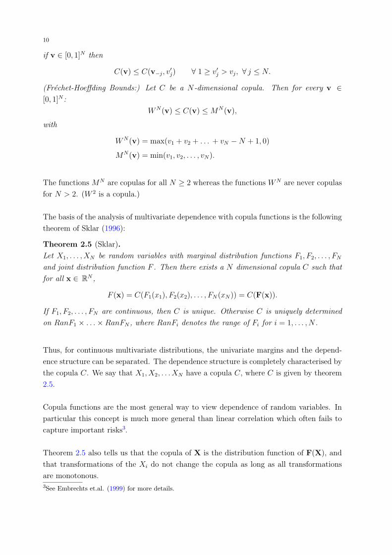
The basis of the analysis of multivariate dependence with copula functions is the following

theorem of Sklar (1996):

Theorem 2.5 (Sklar).

Let X1, . . . , XN be random variables with marginal distribution functions F1, F2, . . . , FN

and joint distribution function F . Then there exists a N dimensional copula C such that

for all x ∈ RN ,

F (x) = C(F1(x1), F2(x2), . . . , FN(xN)) = C(F(x)).

If F1, F2, . . . , FN are continuous, then C is unique. Otherwise C is uniquely determined

on RanF1 × . . .×RanFN , where RanFi denotes the range of Fi for i = 1, . . . , N .

Thus, for continuous multivariate distributions, the univariate margins and the depend-

ence structure can be separated. The dependence structure is completely characterised by

the copula C. We say that X1, X2, . . . XN have a copula C, where C is given by theorem

2.5.

Copula functions are the most general way to view dependence of random variables. In

particular this concept is much more general than linear correlation which often fails to

capture important risks3.

Theorem 2.5 also tells us that the copula of X is the distribution function of F(X), and

that transformations of the Xi do not change the copula as long as all transformations

are monotonous.3See Embrechts et.al. (1999) for more details.

11

Independence of continuous random variables is also easily characterised with their cop-

ula: The X1, X2, . . . , XN are independent if and only if the N -dimensional copula C of

X1, X2, . . . , XN is

C(F(x)) = ΠN(F(x)).

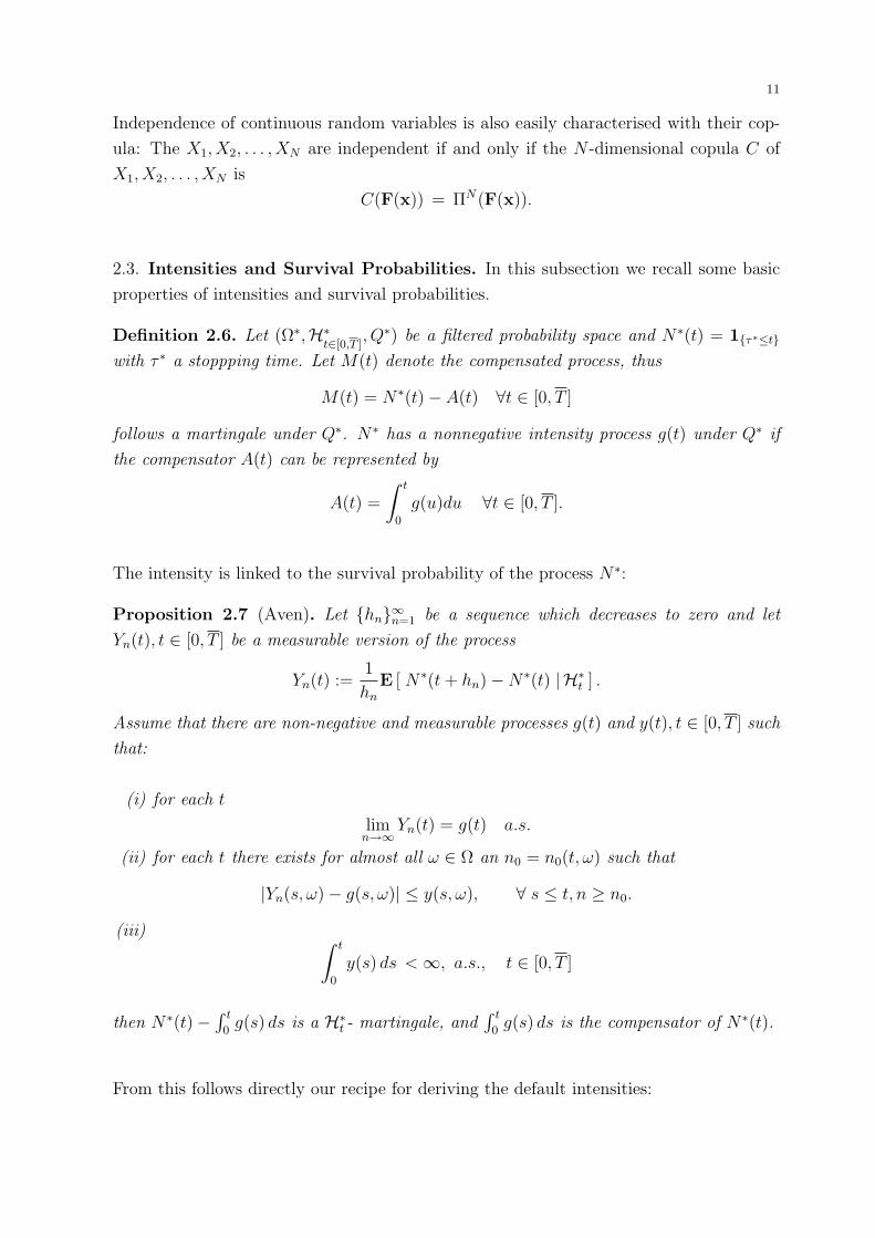
2.3. Intensities and Survival Probabilities. In this subsection we recall some basic

properties of intensities and survival probabilities.

Definition 2.6. Let (Ω∗,H∗t∈[0,T ]

, Q∗) be a filtered probability space and N∗(t) = 1τ∗≤t

with τ ∗ a stoppping time. Let M(t) denote the compensated process, thus

M(t) = N∗(t)− A(t) ∀t ∈ [0, T ]

follows a martingale under Q∗. N∗ has a nonnegative intensity process g(t) under Q∗ if

the compensator A(t) can be represented by

A(t) =

∫ t

0

g(u)du ∀t ∈ [0, T ].

The intensity is linked to the survival probability of the process N∗:

Proposition 2.7 (Aven). Let hn∞n=1 be a sequence which decreases to zero and let

Yn(t), t ∈ [0, T ] be a measurable version of the process

Yn(t) :=1

hn

E [ N∗(t + hn)−N∗(t) |H∗t ] .

Assume that there are non-negative and measurable processes g(t) and y(t), t ∈ [0, T ] such

that:

(i) for each t

limn→∞

Yn(t) = g(t) a.s.

(ii) for each t there exists for almost all ω ∈ Ω an n0 = n0(t, ω) such that

|Yn(s, ω)− g(s, ω)| ≤ y(s, ω), ∀ s ≤ t, n ≥ n0.

(iii) ∫ t

0

y(s) ds < ∞, a.s., t ∈ [0, T ]

then N∗(t)−∫ t

0g(s) ds is a H∗

t - martingale, and∫ t

0g(s) ds is the compensator of N∗(t).

From this follows directly our recipe for deriving the default intensities:

12

Lemma 2.8. Let

P (t, T ) := Q∗ [ τ ∗ > T |H∗t ]

denote the probability given H∗t that the jump has not occured until T . Furthermore let

P (t, T ) be differentiable from the right with respect to T at T = t, and let the difference

quotients that approximate the derivative satisfy the assumptions of proposition 2.7. Then

the intensity of the process N∗ is given by:

(3)dA(t)

dt= g(t) = − ∂

∂T

∣∣∣∣T=t

P (t, T ).

Thus, given certain regularity conditions, we can directly derive the default intensity if

we have the survival probabilities.

3. Model Setup

The dependent-defaults model is built up in two steps: First we specify the stochastic

model for individual defaults, and in a second step we introduce default dependency. In

this section we describe the stochastic model for the defaults of the individual obligors.

We consider an economy with i = 1, . . . , I obligors.

The basic probability space in which the model lives is (Ω, F , Q). Ω is assumed to be

large enough to support all processes that are introduced. All subsequently introduced

filtrations are subsets of F and augmented by the zero-sets of F . The probability measure

Q can – but need not – be a martingale measure for the specific filtrations considered.

First, we introduce the background filtration (Gt)t∈[0,T ]. This filtration represents inform-

ation about the development of general market variables such as share prices, default-free

interest-rates or exchange rates, and also all default-relevant information except explicit

information on the occurrence or non-occurrence of defaults4. Thus, (Gt)t∈[0,T ] can also

contain information on credit spread movements and rating transitions (except for trans-

itions to ’default’). To aid intuition we assume that (Gt)t∈[0,T ] is generated by a stochastic

process X(t), the background process.

Definition 3.1. The background process X(t) is a m-dimensional stochastic process. We

denote the filtration generated by X(t) with (Gt)t∈[0,T ], and G := σ(⋃

t∈[0,T ]

Gt).

Defaults in this model are triggered as follows:

4Mathematically, (Gt)t∈[0,T ] must be independent from all Ui (which will be introduced later).

13

Assumption 1 (Default Mechanism).

The time of default τi of obligor i = 1, . . . , I is the first time, when the default countdown

process γi(t) reaches the level of the trigger variable Ui:

(4) τi := inft : γi(t) ≤ Ui,

where:

(i) The default trigger variables Ui, i = 1, . . . , I are random variables on the unit

interval [0, 1]. σ(Ui) =: Ui is the information generated by knowledge of Ui.

(ii) The pseudo default-intensity λi(t) is a nonnegative cadlag stochastic process which

is adapted to the filtration (Gt)t∈[0,T ] of the background process. Denote Λi(t) :=∫ t

0λi(s)ds the integral of the intensity.

(iii) The default countdown process γi(t) is defined as

(5) γi(t) := exp(−∫ t

0

λi(u) du).

Furthermore we define the default and survival indicator processes Ni(t) := 1τ≤t and

Ii(t) := 1τi>t. Filtration (F it )t∈[0,T ] is the augmented filtration that is generated by Ni(t).

Default of obligor i is triggered as soon as the countdown process γi(t) falls below the

random trigger level Ui. The realisation of this trigger level remains unknown to the

economy, only at default its value is revealed. The pseudo default intensity λi(t) controls

the speed of the countdown and thus the likelihood of an early default. The process λi(t)

is called pseudo default-intensity, because it coincides with the default intensity of obligor

i in the “independence” case described below, or if information is restricted to information

about obligor i alone. In general, it will not be the default intensity.

Usually, the introduction of the threshold levels Ui is not necessary when a totally in-

accessible stopping time is defined, it is sufficient to specify the intensity process which

gives all information on the distribution of the jump times. We introduced the Ui anyway

because they will provide the handle to introduce default dependencies into the model.

Furthermore, this setup directly shows how to efficiently simulate this model in a Monte-

Carlo simulation: Draw the Ui, simulate the paths of λi (and thus γi) and determine the

times of default.

This setup is very general. We deliberately did not restrict the dynamics of the stochastic

processes of the pseudo default-intensities λi to give the reader the freedom to choose

her favourite specification of an intensity model, based upon any of the models that were

14

proposed in the literature. In particular, the dynamics of the pseudo-default intensities

can be correlated or dependent themselves.

The modelling of the default time (4) is inspired by an observation in Lando (1998).

Lando shows that the time of the first jump of a Cox process with intensity λ(u) can be

constructed as

(6) τ = inft :

∫ t

0

λ(u) du ≥ E,

where E is a unit exponential random variable independent of λ. This setup is equivalent

to taking logarithms of both sides of the inequality in equation (4) when Ui is uniformly

distributed on [0, 1]. Almost all practical implementations of intensity-based models can

be translated into a Cox-process framework.

In the analysis of this setup it is crucial to be very careful in the specification of the avail-

able information, because default probabilities will be different, and different information

structures are plausible. We therefore introduce the following filtrations:

Definition 3.2. (i) Filtration (Hit)t∈[0,T ] contains information about the default or sur-

vival of obligor i up to time t, and complete information about the background process

Hit := σ

(F i

t ∪ G).

(ii) Filtration (Hit)t∈[0,T ] contains information about the default or survival of obligor i

up to time t, and partial information about the background process up to time t

Hit := σ

(F i

t ∪ Gt

).

(iii) Filtration (Ht)t∈[0,T ] reflects information about the defaults of all obligors until t,

and complete information about the background process:

Ht = σ

(I⋃

i=1

Hit

).

(iv) Filtration (Ht)t∈[0,T ] is the equivalent of (Ht)t∈[0,T ], but with the information on the

background process restricted to [0, t]

Ht = σ

(I⋃

i=1

Hit

).

(v) Filtration (Ft)t∈[0,T ] contains only default information of all I obligors up to time t

(Ft)t∈[0,T ] = σ

(I⋃

i=1

F it

).

15

Definition 3.2 contains all possible permutations of information sets:

• Filtrations indexed with i contain only information on one obligor.

• Filtrations with a tilde contain full information on the background process X.

This is unrealistic, but useful in the mathematical derivations.

• Filtrations without a tilde only contain information that is available at time t.

In particular, Ht represents all available information in the economy at time t.

Filtration Hit represents all available information if we restrict our attention only

on obligor i and the background process.

These filtrations enable us to model the intensity of the default process of one obligor

independent of the information about the default behaviour of the remaining I−1 obligors.

As shown in the following sections the default process Ni has a different intensity under

the filtration (Hit)t∈[0,T ] than under (Ht)t∈[0,T ]. Accordingly, we need to define different

survival probabilities.

Definition 3.3 (Survival Probabilities).

For each of obligor i, i = 1, . . . , I define

(1) the survival probability until T given the information (Hit)t∈[0,T ]:

P ′i (t, T ) := EQ[Ii(T )|Hi

t],

(2) the survival probability until T given the information (Hit)t∈[0,T ]:

P ′i (t, T ) := EQ[Ii(T )|Hi

t].

The dashes indicate that these probabilities are survival probabilities under the restriction

to the default history of obligor i alone, i.e. ignoring the other obligors.

Next we make our first assumption about the distributions of the Ui, i = 1, . . . , I:

Assumption 2.

For all i = 1, . . . , I, the default threshold Ui is uniformly distributed on [0, 1] under

(Q, Hi0), and Ui is independent from G∞ under Q.

Under this assumption only the marginal distribution of the Ui is prescribed, because

the filtration (Hit)t∈[0,T ] does not contain information about the other Uj. Now we can

calculate the survival probabilities:

16

Proposition 3.4.

Under assumption 2 and given τi > t the survival probabilities are:

P ′i (t, T ) =

γi(T )

γi(t)= e−

∫ Tt λi(s)ds(7)

P ′i (t, T ) = EQ

[γi(T )

γi(t)

∣∣∣∣Hit

]= EQ

[e−

∫ Tt λi(s)ds

∣∣∣Hit

].(8)

Proof. Equation (7):

P ′i (t, T ) = Q

[τi > T

∣∣∣ Hit ∧ τi > t

]= Q

[γi(T ) > Ui

∣∣∣ Hit ∧ τi > t

].

From τi > t we know that Ui < γi(t), thus Ui is uniformly distributed on [0, γi(t)].

Therefore

P ′i (t, T ) =

γi(T )

γi(t).

Equation (8): From Hit ⊂ Hi

t follows for all random variables X:

E[

X |Hit

]= E

[E[

X∣∣∣ Hi

t

] ∣∣∣Hit

].

As stated in lemma 2.8 we can characterize the intensity of the default process through

the survival probabilities.

Proposition 3.5.

The intensity of the process Ni(t) under the filtration (Hit)t∈[0,T ] is

− ∂

∂TP ′

i (t, T )

∣∣∣∣T=t

= 1τ i>tλi(t).

Proof. By differentiation. We can differentiate under the integral sign since the random

variable γi(T )/γi(t) is bounded by 1 and therefore uniformly integrable.

Proposition 3.5 shows, that λi is indeed the default intensity of obligor i, if only this

obligor and the general state of the economy is observed. This proves our claim that by

reducing the information set to (Hit)t∈[0,T ] the model reduces to a standard default risk

model of the intensity-type for a single obligor.

17

4. The joint dynamics of survival probabilities and default intensities

Dependence between the defaults of the I obligors is introduced through the specification

of the joint distribution of the random variables U1, U2, . . . , UI :

Assumption 3.

Under (H0, Q) the I-dimensional vector U = (U1, . . . , UI) is distributed according to the

I-dimensional copula

C(u).

U is independent from G∞. Furthermore, C is twice continuously differentiable.

Because the marginal distributions of a copula function are uniform, this assumption is

consistent with assumption 2. We could also have used a general distribution function on

[0, 1]I but that would have meant giving up the following advantage of uniform margins:

Introducing the joint default distribution via the copula function C(u) does not change

the individual default probabilities if we ignore the other obligors. It also does not change

the default probabilities as seen from t = 0. At later times and given information on the

default- and survival behaviour of the other obligors, this will be different.

It should be pointed out that — besides the dependency between the trigger levels Ui —

the model can also accommodate correlations between the pseudo default-intensities λi(t).

As mentioned in the introduction, this alone would not generate default correlations of a

realistic size, but as an augmentation of our modelling approach it is useful.

Remark 4.1. (i) For every differentiable copula function we have

0 ≤ ∂

∂vi

C(v) ≤ 1 ∀vi ∈ [0, 1], i = 1 . . . , I.

(ii) In the single-obligor case, under (Ht)t∈[0,T ] the distribution function of the time τi of

the default of obligor i is Fi(t) = 1− γi(t).

A similar result now holds in the multi-obligor case: Under (Ht)t∈[0,T ] the joint

distribution function of the times τ = (τ1, . . . , τI) of default is

(9) Q[

τ ≥ t∣∣∣ H0

]= F (t) = C(γ1(t1), . . . , γI(tI)) = C(γ(t)).

As usual, taking the expectation of (9) yields the corresponding distribution function

under (Ht)t∈[0,T ].

We now introduce survival probabilities which are conditioned on events included in the

filtrations (Ht)t∈[0,T ] and (Ht)t∈[0,T ]. In particular we consider two classes of events. In

18

the first case all obligors have survived until time t and in the other case one obligor has

undergone a default at time t.

4.1. Probabilities before defaults.

Definition 4.2.

Survival Probabilities For each obligor i, i ≤ I we define

(1) the survival probability given the information (Ht)t∈[0,T ]:

Pi(t, T ) := EQ [ Ii(T ) |Ht ] ,

(2) the survival probability given the information (Ht)t∈[0,T ]:

Pi(t, T ) := EQ[

Ii(T )∣∣∣ Ht

].

(3) the default intensity hi(t) for information (Ht)t∈[0,T ] and hi(t) for (Ht)t∈[0,T ].

The following is the analogous result to proposition 3.4.

Proposition 4.3.

If no obligor has defaulted until t the individual survival probabilities and default intensities

are

Pi(t, T ) =C(γ−i(t), γi(T ))

C(γ(t))(10)

Pi(t, T ) = EQ

[C(γ−i(t), γi(T ))

C(γ(t))

∣∣∣∣Ht

](11)

hi(t) = hi(t) = λi(t)γi(t)∂

∂xiC(γ(t))

C(γ(t))= λi(t)γi(t)

∂

∂xi

ln C(γ(t)).(12)

Proof. Apply Bayes’ rule (for the conditioning on survival until t) and assumption 3.

Differentiate to reach the default intensity. As hi(t) only depends on quantities that are

Ht-measurable, the default intensities under (Ht)t∈[0,T ] and (Ht)t∈[0,T ] coincide. (This is

no surprise given the local character of the default intensity.)

The intensity hi(t) still depends on the one-obligor intensity λi(t) from proposition 3.5,

but it is modified. This modification reflects the fact, that under the filtration (Ht)t∈[0,T ]

we are able to observe more information on the default likelihood of obligor i than under

filtration (Hit)t∈[0,T ]. The additional information is the information, that the other obligors

have not defaulted yet, it is information on Ui than can be inferred from U−i < γ−i(t).

19

If the Ui are independent, observing the survival and defaults of the other obligors does

not convey information on obligor i. If the copula in proposition 4.3 is the independence

copula ΠI() then

(13) hi(t) = λi(t) ∀ i ≤ I.

The intensities hi(t) and λi(t) also coincide at t = 0: Here the partial derivatives of C

coincide with the marginal derivatives Cxi(1) = 1.

It is easy to check that λi(t) is recovered as intensity if we artificially restrict our inform-

ation to Hit. Thus

(14) λi(t) = EQ[

hi(t)∣∣∣ (Hi

t)t∈[0,T ]

]∀ i ≤ I,

a single-obligor default risk model can be viewed as the projection of a multi-obligor

default risk model onto the one-obligor world. The same results apply to the survival

probabilities Pi(t, T ) and P ′i (t, T ).

4.2. Probabilities after defaults. If one or more of the obligors have already defaulted,

we move to a conditional distribution function. If obligor i defaults at time t, we have

to use the conditional distribution of the U from that time onwards, conditional on

Ui = γi(t). This function is given in the following lemma:

Lemma 4.4. Assume the times of default of k < I obligors are known at time t. W.l.o.g.

we assume that these are the first k obligors. If C is sufficiently differentiable, the condi-

tional distribution function of τ is

Q[

τ ≥ T∣∣∣ Ht ∧ τi = ti for 1 ≤ i ≤ k ∧ τj > t for k < j ≤ I

]=

∂k

∂x1···∂xkC(γ1(t1), . . . , γk(tk), γk+1(Tk+1), . . . , γI(TI))

∂k

∂x1···∂xkC(γ1(t1), . . . , γk(tk), γk+1(t), . . . , γI(t))

,(15)

and

Q [ τ ≥ T |Ht ∧ τi = ti for 1 ≤ i ≤ k ∧ τj > t for k < j ≤ I ]

=EQ[

∂k

∂x1···∂xkC(γ1(t1), . . . , γk(tk), γk+1(Tk+1), . . . , γI(TI))

∣∣∣Ht

]∂k

∂x1···∂xkC(γ1(t1), . . . , γk(tk), γk+1(t), . . . , γI(t))

,(16)

where Ti > τi for i ≤ k.

Apart from a different form for the distribution function of the Ui the situation is now

identical to the situation before any defaults in the previous subsection. Thus, the survival

20

probabilities and default intensities of the remaining obligors are reached by substituting

the conditional distribution function (15) as distribution function in proposition 4.3.

The conditional distribution function is actually not a copula function but just a general

distribution function on the unit hypercube (with non-uniform marginals): To reach a

copula distribution function again we need to transform the γi with the respective marginal

distribution functions. This is not really necessary because the uniform marginals were

only used to conveniently reduce the model to the one-obligor case.

4.3. Probabilities at defaults. Because we assumed C to be differentiable, joint de-

faults at exactly the same time have probability zero in this model. Thus, fundamentally

there are only two types of points in time: Points when no default occurs, and points

in time when a default happens. The survival probabilities and default intensities in the

standard case (no default) were given in the previous proposition. Now we analyze what

happens to the survival probabilities of the other obligors at the time of default of an

obligor j. At this point in time the distribution of default times changes discretely to the

conditional distribution function according to lemma 4.4.

Definition 4.5.

Survival Probabilities given default For each obligors i and j, i, j = 1, . . . , I define

(1) the survival probability of i given the information (Ht)t∈[0,T ] and given a default of

obligor j at t:

P−ji (t, T ) := EQ [ Ii(T ) |Ht ∧ τj = t ] ,

(2) the survival probability of i given the information (Ht)t∈[0,T ] and given a default of

obligor j at t:

P−ji (t, T ) := EQ

[Ii(T )

∣∣∣ Ht ∧ τj = t],

Using equation (15) these survival probabilities take the following values: (We will now

use subscript notation for partial derivatives of C, i.e. Cxi= ∂

∂xiC etc.)

Proposition 4.6.

If obligor j has defaulted at t and all other obligors are still alive at t, the individual

21

survival probabilities and default intensities are for obligor i

P−ji (t, T ) =

Cxj(γ−i(t), γi(T ))

Cxj(γ(t))

(17)

P−ji (t, T ) = EQ

[Cxj

(γ−i(t), γi(T ))

Cxj(γ(t))

∣∣∣∣Ht

](18)

h−ji (t) = λi(t)γi(t)

Cxixj(γ(t))

Cxj(γ(t))

.(19)

Comparing this to the survival probabilities in proposition 4.3, we see that the survival

probabilities after a default of obligor j now use the conditional distribution function of

the Ui. The partial derivative is taken w.r.t. the defaulted obligor j in the copula function,

and the j-th argument of the copula is set to γj(t) at t = τj (and it also remains at γj(τj)

at later times).

Except in the independence case, the new default intensity of i will not be equal to the

default intensity of i before the default of j. The change to the conditional distribution

will result in a jump in the default intensity and in the survival probabilities. This effect

is quantified in the next subsection.

4.4. Dynamics of default intensities. If the pseudo-default intensities λi follow diffu-

sion processes, the dynamics of the default intensities hi follow directly from Ito’s lemma:

Proposition 4.7.

If no default has happened until time t, the dynamics of the default intensity hi are given

by

dhi =Cxi

C· γiλi ·

[(dλi

λi

− λi dt

)−

I∑j=1

(Cxixj

Cxi

−Cxj

C

)γjλj dt

],(20)

if there is no default at t, and a jump of

∆hi = λiγiCxi

C

[Cxjxi

C

CxjCxi

− 1

](21)

if obligor j 6= i defaults at time t. (Suppressing the arguments t and γ(t).)

This can be re-written as:

dhi

hi

=dλi

λi

+ (hi

(1− Cxixi

C

C2xi

)− λi)dt− dNi +

I∑j=1, j 6=i

(Cxixj

C

CxiCxj

− 1

)(dNj − hjdt).

(22)

22

Equation (22) has the following interpretation: First, the default intensity hi of obligor i

is driven by the pseudo default intensity λi. This is the only source of diffusion risk in hi,

in particular we will have the same volatility for λi and hi. The next term is a correction

term for the fact that in general λi 6= hi and that C is not linear in xi. Then follows −dNi

which sets hi to zero after the default of obligor i.

The influence of potential defaults of other obligors is contained in the summation term

in equation (22). This term is of the form of a compensated jump process: There is a

large jump component (triggered by dNj = 1) at a default of obligor j.

The sign of the jump is determined by the dependence between the default times of i and

j. A common measure for the dependence between two random variables X and Y is

Kendall’s tau. It can be written as

(23) ρτ = 2

∫[0,1]2

C(u, v)Cuv(u, v)− Cu(u, v)Cv(u, v)du dv,

where C(u, v) is the copula function of X and Y . (See Durrleman et.al. (2000).) From

equation (23) follows directly, that a positive sign of the jump terms in proposition 4.7

corresponds to a positive contribution to Kendall’s tau, and thus to a locally positive

dependence between Ui and Uj.

If there is positive (negative) dependence between the defaults of obligors i and j then

the survival probability of i will drop (increase) at a default of j, for independence it

remains unchanged. If on the other hand obligor j survives over the infinitesimal interval

[t, t + dt] then this will have the opposite effect of a default on the intensity of i. Survival

of j means that a default of i is less (more) likely if i and j are positively (negatively)

dependent.

5. Examples

5.1. Archimedean Copulas. A popular class of copula functions are the Archimedean

copula functions which have the following representation:

Definition 5.1 (Archimedean Copulas).

An Archimedean copula function is a copula function which has the following representa-

tion:

C(x) = φ[−1]( I∑

i=1

φ(xi)).

23

The function φ(·) is called the generator of the copula, φ[−1] denotes the inverse function

of φ.

The generator has the following properties5: φ : [0, 1] → R+ ∪ +∞, φ is invertible,

φ′(x) < 0, φ′′(x) > 0. Archimedean copulas are capable of reproducing a large variety of

possible dependence structures.

It is straightforward to check that for an Archimedean copula C with generator φ the

partial derivatives with respect to xi and xj, i, j ≤ I are given by

Cxi(x) =

φ′(xi)

φ′(C(x))Cxixj

(x) = −φ′(xi)φ′(xj)

φ′′(C(x))

(φ′(C(x)))3.

Thus we reach the following proposition:

Proposition 5.2. If the distribution function C of the Ui is an Archimedean copula

function with generator φ, then for any obligor i ≤ I

(a) the default intensity before any defaults is

hi(t) =φ′(γi)

C(γ)φ′(C(γ))γiλi,

(b) at default t = τj of obligor j 6= i the default intensity changes by a factor

h−ji (t) = hi

(−C(γ)φ′′(C(γ))

φ′(C(γ))

),

(c) the dynamics of hi are

dhi

hi

=dλi

λi

− λidt−(−Cφ′′(C)

φ′(C)

)dNi +

I∑j=1

((−Cφ′′(C)

φ′(C)

)− 1

)(dNj − hjdt).

In particular, the symmetric nature of the Archimedean copula functions has the effect

that at a default of an obligor j, the default intensities of all other obligors change by

the same factor. The default risk of obligor i depends on only two components: The

individual default risk which is represented by φ′(γi), and the default dependency which

can be summarised by C(γ).

5.2. Gumbel and Clayton Copulae.

Definition 5.3 (Gumbel Copula).

With φ(x) = (− ln(x))θ for θ ∈ [1,∞) in definition 5.1 we reach the one-parameter Gumbel

5These conditions are necessary, but not sufficient for φ to be a generator of a I-copula.

24

copula:

C(x) = exp

−[

I∑i=1

(− ln xi)θ

] 1θ

.

The generator of the Clayton copula is φ(x) = (x−α − 1)/α for α > 0. Then

C(x) =

(1− I +

I∑i=1

x−αi

)− 1α

.

The interesting quantities in proposition 5.2 are the default intensity hi and the jump in

the default intensity of i if j defaults. These are for the Gumbel copula

hi(t) =φ′(γi)

C(γ)φ′(C(γ))γiλi, =

(Λi

‖Λ‖θ

)θ−1

λi(24)

h−ji (t) =

(−C(γ)φ′′(C(γ))

φ′(C(γ))

)hi, =

(1 +

(θ − 1)

‖Λ‖θ

)hi(25)

and for the Clayton copula

hi(t) =φ′(γi)

C(γ)φ′(C(γ))γiλi, =

(C(γ)

γi

)α

λi(26)

h−ji (t) =

(−C(γ)φ′′(C(γ))

φ′(C(γ))

)hi = (1 + α)hi.(27)

where we wrote ‖x‖θ :=(∑I

i=1 |xi|θ) 1

θfor the θ-norm in RI and Λi(t) :=

∫ t

0λi(s)ds.

With the Clayton copula we regain a feature of the Davis/Lo (1999a; 1999b) model: A

jump in the credit spread by a constant factor (1+α) at a default of another obligor. The

copula approach yields several new insights into that model: The corresponding copula

is the Clayton copula function, and we can directly give the distribution of the default

times. Furthermore, we now can transform the model to a fixed time-horizon model which

greatly facilitates the estimation of the parameter α. There are some differences in the

details of the model, e.g. Davis and Lo suggest to let the increased hazard rate return

to pre-default levels after an exponentially distributed crisis period, while here there is

the drift correction to the default intensity which tends to reduce the default intensities

continuously as long as no default happens.

For the Gumbel copula, the intensity hi(t) depends on the factor Λi(t)‖Λ(t)‖θ

, which represents

the dependence structure of the default times. This is the i-th component of the cumulat-

ive intensity-vector Λ, normalized to one in the θ-norm. For constant pseudo-intensities

λi this factor will be constant, thus making the model time-invariant before defaults. In

25

contrast to this, the jump factor when a default happens is not constant but approaches

1 as time proceeds, thus preventing the default intensities from increasing too much.

5.3. Estimation, Gaussian Copula and Credit Metrics. It is well-known that port-

folio default-risk models like CreditMetrics have a Gaussian copula structure if they are

based upon the Merton (1974) firm’s value model. These models are usually calibrated

to the historical default experience of a country or industry group over a given (e.g. one-

year) time horizon. It may be argued that a copula of default events over a one-year

horizon would look different from a copula of default-times as it is used in this model.

This is not the case because copula functions are invariant under monotonic increasing

transformations of the marginals (see e.g. Li, Credit Metrics Monitor or Joe (1997)). If

the transformation is monotonically decreasing, the copula of the transformed variables

is equal to the survival copula of the original variables. For many important cases (e.g.

Gaussian copula, t−copula), the survival copula is identical to the original copula.

We now show, that we can indeed directly derive the copula C(·) that we use in the model

from historically observed default frequencies.

The indicator function of survival beyond the time-horizon T can be approximated arbit-

rarily well by continuously differentiable function, for example cumulative normal distri-

bution functions:

1τi>Ti = limn→∞

gn,Ti(τi) =: lim

n→∞N

(τi − Ti

n

).

For all n, gn,Ti(·) is a strictly monotonically increasing function. Call Cg,n,T(·) the copula

function of the random variables Yi,n := gn,Ti(τi). By the invariance of copulae under

strictly monotonous transformations, Cg,n,T(·) will be equal to the copula of the default

times Cτ (·) for all n and for all choices of transformation function g and time horizons Ti.

Analogously, if instead of survival indicators, we construct default indicators, we reach

the survival copula of the default times. Again this result will hold independently of n

or the approximation functions g or time horizons Ti. Thus, the copula will remain valid

even if the limit is taken as n →∞.

On the other hand, by construction, the copula function C(·) of the model is the cop-

ula function of yet another transformation of the default times. By (9), the survival

probabilities are given by

Q[

τ ≥ t∣∣∣ H0

]= F (t) = C(γ1(t1), . . . , γI(tI)) = C(γ(t)).

Thus, the model copula C(·) is the survival copula of the default-time copula Cτ (·).

26

In the limit as n →∞, the approximated default indicator functions will approach the de-

fault indicator functions themselves. We can therefore use a fixed-horizon default copula

function in our model, for example the Gaussian default copula function of the Credit-

Metrics model.

The Gaussian copula is not in the class of Archimedean copula functions and the terms in

propositions 4.3, 4.4 and 4.6 do not simplify nicely, so we refrain from stating them here.

Sampling from a Gaussian copula is very easy, though, so this should not be an obstacle

to the numerical implementation of the model.

If a CreditMetrics (or similar) Gaussian correlation matrix R for the values of the assets

of the obligors is given, random samples from the corresponding copula function can be

drawn according to the following algorithm:

(1) Draw X, a vector of I standard normal random variates which have the correlation

matrix R

(2) Yi := N [−1](Xi), i ≤ I have the corresponding Gaussian copula as distribution.

(N [−1] is the inverse of the standard normal distribution function.)

The time-transformation argument applies to all copula functions. Therefore, the choice

of an appropriate copula and the estimation of its parameters can all be achieved by

analysing default frequencies over a given time-horizon. Alternatively, one can try to

fit the jump sizes of the spreads at a given default to historical experience or personal

intuition. Even if one does not want to calibrate the model to the jump sizes at default,

it is still advisable to use them for a plausibility check.

6. Defaultable bond pricing

In this section we describe briefly how the copula-approach can be used to link several

single-name intensity models with the default copula, and how to calibrate the result-

ing model. To simplify the exposition we will only consider the pricing of defaultable

zero coupon bonds under zero recovery, for a serious implementation we recommend the

’recovery of par’ model as it is described in Duffie (1998a) and Schonbucher (1999). In

these models, prices of defaultable zero-coupon bonds with zero recovery are the central

ingredient to which the model is calibrated.

27

Assume that we have I independent intensity-based models that are calibrated to the term

structure of default risk of our obligors. I.e. we have found dynamics for the processes

λi(t) such that the fit to the initial term structure of defaultable bond prices Bi(0, T ) is

achieved for all T ≥ 0, i ≤ I:

(28) Bi(0, T ) = EQ[

e−∫ T0 r(s)ds1τi>T

∣∣∣Hi0

]= EQ

[e−

∫ T0 r(s)dse−

∫ T0 λi(s)ds

∣∣∣Hi0

].

For simplicity, these models are set in the Cox-process framework of section 3.

To embed these models into a copula model with dependent defaults we define the back-

ground filtration G∞ is the union of the individual background filtrations and the filtration

generated by the interest-rate process. As described earlier, the defaults are generated

with the default countdown processes, with copula-dependent trigger levels Ui.

It remains to be shown that in this general model the initial term structures of defaultable

bond prices remain indeed calibrated. This follows from

Bi(0, T )?= EQ

[e−

∫ T0 r(s)ds1τi>T

∣∣∣H0

]using iterated expectations yields

= EQ[EQ[

e−∫ T0 r(s)ds1τi>T

∣∣∣ Hi0

] ∣∣∣H0

]the discount factor is measurable with respect to the inner filtration, so

= EQ[

e−∫ T0 r(s)dsEQ

[1τi>T

∣∣∣ Hi0

] ∣∣∣H0

]the survival probability follows from the results earlier in the paper

= EQ[

e−∫ T0 r(s)dsγi(T )

∣∣∣H0

]and this expectation just depends on the background processes and not the copula struc-

ture, therefore we reach

= Bi(0, T ),

as claimed.

Thus, the calibration of the dynamics of the pseudo-default intensity processes λi to

reproduce given term structures of defaultable bond prices will in fact mean that the

copula-dependent default risk model will also be calibrated to these initial term structures.

28

This connection is only valid at t = 0, because it uses the uniform marginal distributions

of the copula function C. If the term structure of defaultable bond prices is to be recovered

at a later time, then one must use the conditional distribution of the Ui which will not

have uniform margins. This will not be a problem because the probabilities are directly

given through the copula.

7. Conclusion

The setup of the model directly gives the strategy for an implementation via Monte-Carlo

simulation: First, the default trigger-levels are drawn according to the copula distribution

function, then the intensities and interest-rate processes are drawn independently.

It is also possible to invert the order of the simulation procedure: First simulate the paths

of interest-rates and intensities, and then simulate the trigger levels and times of default.

As the trigger levels are independent from the rest of the model, the second step can be

repeated several times. This can lead to a significant saving in simulation time, because

the realisation of the trigger levels Ui usually causes the largest variance in the sample,

while the simulation of the paths of intensities and rates costs most computer time. This

is subject to further research.

The copula model for default dependency in this paper achieves several goals: It builds

on existing intensity-based models for individual default risk, its calibration to individual

term structures of credit spreads and credit spread volatilities is straightforward, for the

calibration of the default dependency historical observations can be used in a direct way.

Furthermore the model links naturally with portfolio credit risk models like CreditMetrics.

The dynamics of the model are realistic, too: Credit spread changes at credit crises happen

in an endogenous and intuitive way, and a realistic time-distribution of the times of default

is achieved. Existing portfolio credit-risk models of the intensity-type were only partially

able to achieve these goals.

These features of the model make it ideally suited to the analysis of the pricing and

hedging of basket default swaps and CDOs and counterparty risk in credit derivatives.

29

References

T. Aven. A theorem for determining the compensator of a counting process. Scandinavian

Journal of Statistics, 12(1):69–72, 1985.

Barry Belkin, Stephan Suchover, and Lawrence Forest. A one-parameter representation

of credit risk and transition matrices. Credit Metrics Monitor, 1(3):46–56, 1998.

Credit Suisse First Boston. Credit Risk+. Technical document, Credit Suisse First Boston,

1997. URL: www.csfb.com/creditrisk.

Michel Crouhy, Dan Galai, and Robert Mark. A comparative analysis of current credit

risk models. Journal Of Banking And Finance, 24(1-2):59–117, January 2000.

Mark Davis and Violet Lo. Infectious defaults. Working paper, Imperial College, London,

1999a.

Mark Davis and Violet Lo. Modelling default correlation in bond portfolios. In Carol

Alexander, editor, ICBI Report on Credit Risk, 1999b.

Mark Davis and Violet Lo. Modelling default correlation in bond portfolios. Working

paper, Imperial College, London, 2000.

Darrell Duffie. Defaultable term structure models with fractional recovery of par. Working

paper, Graduate School of Business, Stanford University, 1998a.

Darrell Duffie. First-to-default valuation. Working paper, Graduate School of Business,

Stanford University, 1998b.

Darrell Duffie and Nicolae Garleanu. Risk and valuation of collateralized debt obligations.

Working paper, Graduate School of Business, Stanford University, 1999.

Darrell Duffie and Kenneth J. Singleton. Modeling term structures of defaultable bonds.

The Review of Financial Studies, 12(4):687–720, 1999.

V. Durrleman, A. Nikeghbali, and T. Roncalli. A simple transformation of copulas. Work-

ing paper, Groupe de Recherce Operationelle, Credit Lyonnais, France, July 2000.

Paul Embrechts, Alexander McNeal, and Daniel Straumann. Correlation and dependence

in risk management: Properties and pitfalls. Working paper, Risklab ETH Zurich,

1999.

Christopher C. Finger. Conditional approaches for credit metrics portfolio distributions.

Credit Metrics Monitor, 2(1):14–33, April 1999.

Rudiger Frey and Alexander J. McNeil. Modelling dependent defaults. working paper,

Department of Mathematics, ETH Zurich, March 2001.

John Hull and Alan White. Valuing credit default swaps II: Modeling default correlations.

Journal of Derivatives, 8(3):12–22, Spring 2001.

Robert A. Jarrow and Stuart M. Turnbull. Pricing derivatives on financial securities

subject to credit risk. Journal of Finance, 50:53–85, 1995.

30

Robert A. Jarrow and Fan Yu. Counterparty risk and the pricing of defaultable securities.

Working paper, Johnson GSM, Cornell University, 2000.

Harry Joe. Multivariate Models and Dependence Concepts, volume 37 of Monographs on

Statistics and Applied Probability. Chapman and Hall, London, Weinheim, New York,

1997.

JPMorgan & Co. Inc. Credit Metrics. Technical document, JPMorgan & Co. Inc., 1997.

URL: www.creditmetrics.com.

Masaaki Kijima. Valuation of a credit swap of the basket type. Review of Derivatives

Research, 4:81–97, 2000.

David Lando. On Cox processes and credit risky securities. Review of Derivatives Re-

search, 2(2/3):99–120, 1998.

David. X. Li. On default correlation: A Copula function approach. working paper 99-07,

Risk Metrics Group, April 2000.

Andre Lucas, Pieter Klaassen, Peter Spreij, and Stefan Staetmans. An analytic approach

to credit risk of large corporate bond and loan portfolios. Research Memorandum

1999-18, Vrije Universiteit Amsterdam, February 1999.

Dilip Madan and Haluk Unal. Pricing the risks of default. Review of Derivatives Research,

2(2/3):121–160, 1998.

Yukio Muromachi Masaaki Kijima. Credit events and the valuation of credit derivatives

of basket type. Review of Derivatives Research, 4:55–79, 2000.

Robert C. Merton. On the pricing of corporate debt: The risk structure of interest rates.

Journal of Finance, 29:449–470, 1974.

Roger B. Nelsen. An introduction to copulas, volume 139 of Lecture Notes in Statistics.

Springer, Berlin, Heidelberg, New York, 1999.

Philipp Schonbucher. A libor market model with default risk. Working paper, University

of Bonn, 1999.

Philipp J. Schonbucher. Term structure modelling of defaultable bonds. Review of De-

rivatives Research, 2(2/3):161–192, 1998.

A. Sklar. Random variables, distribution functions, and copulas – a personal look back-

ward and forward. In Ludger Ruschendorf, Berthold Schweizer, and Michael D. Taylor,

editors, Distributions with Fixed Marginals and Related Topics, pages 1–14. Hayward

California, 1996.

Oldrich Vasicek. Probability of loss on loan portfolio. Working paper, KMV Corporation,

1987.