dynamic copula models and high frequency datapublic.econ.duke.edu/~ap172/de_lira_salvatierra... ·...
TRANSCRIPT
Dynamic Copula Models and High Frequency Data�
Irving De Lira Salvatierra and Andrew J. Patton
Duke University
This version: 26 August 2014
Abstract
This paper proposes a new class of dynamic copula models for daily asset returns that exploits
information from high frequency (intra-daily) data. We augment the generalized autoregressive
score (GAS) model of Creal, et al. (2013) with high frequency measures such as realized correlation
to obtain a �GRAS�model. We �nd that the inclusion of realized measures signi�cantly improves
the in-sample �t of dynamic copula models across a range of U.S. equity returns. Moreover, we
�nd that out-of-sample density forecasts from our GRAS models are superior to those from simpler
models. Finally, we consider a simple portfolio choice problem to illustrate the economic gains from
exploiting high frequency data for modeling dynamic dependence.
Keywords: Realized correlation, realized volatility, dependence, forecasting, tail risk.
J.E.L. codes: C32, C51, C58.�We thank Tim Bollerslev, Jia Li, George Tauchen, and seminar participants at Duke for helpful comments. An
appendix containing additional results for this paper is available at http://www.econ.duke.edu/sap172/research.html.Contact address: Andrew Patton, Department of Economics, Duke University, 213 Social Sciences Building, Box90097, Durham NC 27708-0097. Email: [email protected].
1 Introduction
This paper proposes a class of models to incorporate high frequency (intra-daily) information into
models of the dynamic dependence between lower frequency (e.g., daily) asset returns, modeled
using a copula-based approach. Our approach is based on a combination of recent work on general
time-varying distributions (Creal, et al. (2013)), on the incorporation of high frequency data into
models for lower frequency conditional second moments (Shephard and Sheppard (2010), Noureldin
et al. (2012), Hansen et al. (2011, 2013)), and on dynamic copula models for economic time series
(see Patton (2013) for a review).
Unlike variances and covariances, the copula of low frequency returns is not generally a known
function of the copula of corresponding high frequency returns. Thus the elegant link between high
frequency volatility measures (e.g., realized variance and covariance) and their lower frequency
counterparts cannot generally be exploited when considering dependence via the copula function.1
However, it is still likely that high frequency measures such as realized correlation contain infor-
mation that is useful for modeling dynamic dependence through a copula model, to the extent
that the copula model has parameters that are related to correlation. As Andersen, et al. (2003)
note, �[t]he essence of forecasting is quanti�cation of the mapping from the past and present into
the future. Hence, quite generally, superior estimates of present conditions translate into superior
forecasts of the future.�It is this intuition that we seek to exploit in this paper.
Similar to the class of �GARCH-X�models, we propose augmenting a generalized autoregressive
score model (GAS) of Creal et al. (2013) with realized measures such as realized correlation. We call
such models �GRAS�models.2 In addition to a baseline GRAS model using realized correlation,
we also consider models that incorporate realized volatilities, measures of co-jumps, and market
volatility. We apply these models stock returns over the period 2000 to 2010, a total of 2,773 trading
days, and we consider three pairs of stocks, exhibiting low, medium and high levels of correlation.
1The literature on realized measures is large and still growing, see Andersen et al. (2006) and Barndor¤-Nielsenand Shephard (2007) for surveys.
2The name �GAS-X� is already taken for a line of medications. (We thank Drew Creal and Kevin Sheppard forpointing this out to us.)
1
We compare our proposed GRAS copula models with models that do not exploit high frequency
data, both in-sample and out-of-sample. In sample, we �nd that including a measure of realized
correlation signi�cantly improves the performance of the model. This �nding is robust across all
three pairs of assets, across the particular choice of realized measure, and across the �shape�of the
copula that we assume. (We consider the Normal, rotated Gumbel and the Student�s t copulas.)
We also �nd evidence that other high frequency measures, such as continuous and jump realized
correlations and realized volatilities, contain useful information.
We compare the out-of-sample performance of the competing models in two ways. Firstly, we
use the density forecast accuracy test for copulas proposed by Diks et al. (2012). We compare
the dynamic copula models both in terms of their �t across the entire support, and in particular
on the joint tails of the distribution. When we look at the joint tails of the support, the GRAS
model uniformly out-performs the constant parameter copula model and the GAS model, and in
a majority of comparisons the di¤erence is statistically signi�cant. Second, we consider a simple
portfolio decision problem, where a risk averse investor uses one of the competing copula-based
density forecasts to compute her optimal portfolio weights, as in Patton (2004) and Jondeau and
Rockinger (2012). We evaluate the out-of-sample utility of these portfolios, and �nd that investors
are generally willing to pay a positive management fee to switch from the constant copula model
and GAS model to the GRAS model.
This paper is related to work over the past decade on speci�cations for time-varying conditional
copulas. We build on Patton (2006a), Jondeau and Rockinger (2006) and Creal, et al. (2013), who
consider models of time-varying copulas where a parametric functional form is assumed, and the
parameter is allowed to vary through time as a function of lagged information, similar to the ARCH
model for volatility, see Engle (1982).3 We attempt to bridge the gap between the existing time-
varying copula models, which have almost exclusively used lower frequency data, and models from
the volatility and correlation forecasting literature, which have successfully used high frequency
data, see Shephard and Sheppard (2010), Noureldin et al. (2012), Hansen et al. (2011, 2013) for
3Alternative dynamic speci�cations include regime switching models, see Rodriguez (2007) and Okimoto (2008),and �stochastic copula�models, see Hafner and Manner (2010).
2

example. In a recent related paper, Fengler and Okhrin (2012) use a method-of-moments approach
to match the covariance structure implied by a copula-based multivariate model with that estimated
using high frequency data. This approach su¤ers from the fact that it cannot be used with copulas
that have more than one free parameter (e.g., the Student�s t copula), and the authors�simulation
study suggests that it can lead to biased estimators when the level of dependence is high. Our
proposed approach overcomes these limitations by using the GAS structure, described in the next
section, to link high frequency information to low frequency dependence measures.
The remainder paper is organized as follows. Section 2 provides the general formulation of our
GRAS models and outlines the estimation procedure. Section 3 presents our in-sample results,
and Section 4 presents the out-of-sample forecasting results, for density forecasting and a portfolio
choice problem. Section 5 concludes. An online supplemental appendix contains additional details
and results.
2 Dynamic copula models and high frequency data
The models used in this paper are based on Sklar�s (1959) theorem, extended to apply to conditional
distributions in Patton (2006a). This theorem allows the researcher to decompose a (conditional)
joint distribution into marginal distributions and a copula. If Yt = [Y1t; Y2t]0 has conditional joint
distribution Ft and conditional marginal distributions F1t and F2t; then we can write:
YtjFt�1 s Ft = Ct (F1t; F2t) (1)
where Ct is the conditional copula of Yt and Ft�1 is some information set, usually taken as
� (Yt�1;Yt�2; :::) : The copula contains all information about the dependence between Y1t and Y2t;
and is sometimes called the �dependence function.�From a modeling perspective, the usefulness of
Sklar�s theorem arises from the fact that we can construct a joint distribution Ft by linking together
any two marginal distributions, F1t and F2t; with any copula; there is no need for these functions to
belong to the same family. Thus it provides a great deal of �exibility in modeling joint distributions.
3

In Section 2.3 we describe the models that we use for the conditional marginal distributions in our
empirical work, and below we describe various models for the conditional copula. The discussion
below exploits the fact that the conditional copula of Yt can be interpreted as the conditional joint
distribution of the probability integral transforms of these variables:
Let Uit � Fit (Yit) , i = 1; 2 (2)
then UtjFt�1 s Ct
2.1 The GAS model
As noted above, we build on ARCH-type models for the dynamic copula, and in particular the class
of GAS models proposed by Creal, et al. (2013). The GAS speci�cation addresses the problem of
the choice of �forcing variable�to use in the equation governing the dynamics of the time-varying
parameter. For models of the conditional variance, an immediate choice for this variable is the
lagged squared residual, as in the ARCH model, but for models with parameters that lack an
obvious interpretation the choice is less clear. Creal, et al. (2013) propose using the lagged score
of the density model (copula model, in our application) as the forcing variable.4 Speci�cally, for a
copula with time-varying parameter �t we have:
Let UtjFt�1 s C(�t)
then �t = ! + ��t�1 + �st�1 (3)
where st�1 = St�1rt�1
rt�1 =@ log c(ut�1; �t�1)
@�t�1
and St is a scaling matrix (e.g., the inverse Hessian or its square root). While this speci�cation for
the evolution of a time-varying parameter is somewhat arbitrary, Creal, et al. (2013) motivate it
4Harvey (2013) and Harvey and Sucarrat (2012) propose a similar method for modeling time-varying parameters,which they call a �dynamic conditional score,�or �DCS,�model.
4
by showing that it nests a variety of popular and successful existing models: GARCH (Bollerslev
(1986)) for conditional variance; ACD (Engle and Russell (1998)) for models of trade durations (the
time between consecutive high frequency observations); Davis, et al.�s (2003) model for Poisson
counts. Harvey (2013) further motivates this speci�cation as an approximation to a �lter for a
model driven by a stochastic latent parameter, or an �unobserved components�model.
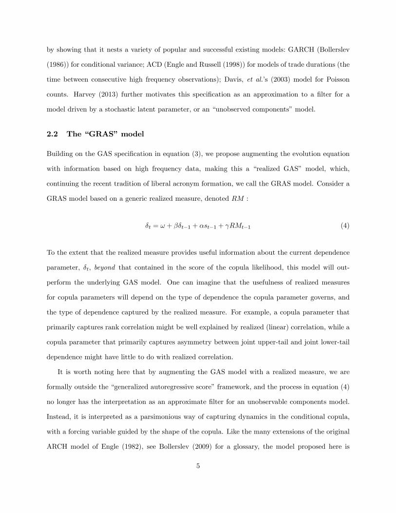
2.2 The �GRAS�model
Building on the GAS speci�cation in equation (3), we propose augmenting the evolution equation
with information based on high frequency data, making this a �realized GAS� model, which,
continuing the recent tradition of liberal acronym formation, we call the GRAS model. Consider a
GRAS model based on a generic realized measure, denoted RM :
�t = ! + ��t�1 + �st�1 + RMt�1 (4)
To the extent that the realized measure provides useful information about the current dependence
parameter, �t; beyond that contained in the score of the copula likelihood, this model will out-
perform the underlying GAS model. One can imagine that the usefulness of realized measures
for copula parameters will depend on the type of dependence the copula parameter governs, and
the type of dependence captured by the realized measure. For example, a copula parameter that
primarily captures rank correlation might be well explained by realized (linear) correlation, while a
copula parameter that primarily captures asymmetry between joint upper-tail and joint lower-tail
dependence might have little to do with realized correlation.
It is worth noting here that by augmenting the GAS model with a realized measure, we are
formally outside the �generalized autoregressive score�framework, and the process in equation (4)
no longer has the interpretation as an approximate �lter for an unobservable components model.
Instead, it is interpreted as a parsimonious way of capturing dynamics in the conditional copula,
with a forcing variable guided by the shape of the copula. Like the many extensions of the original
ARCH model of Engle (1982), see Bollerslev (2009) for a glossary, the model proposed here is
5

somewhat arbitrary, and must be judged on its empirical performance. Sections 3 and 4 are
devoted to answering that question in detail.
Most parametric copulas have parameters that are constrained to lie in a particular range of
values (e.g., a correlation parameter forced to take values only inside (�1; 1)). To ensure that this
is satis�ed, Creal, et al. (2013) suggest applying a strictly increasing transformation, h ; (e.g., log,
logistic, arc tan, etc.) to the parameter,
't = h (�t), �t = h�1 ('t) (5)
and to model the unconstrained transformed parameter, denoted 't. This approach extends directly
to GRAS models and we employ this in our analysis below:
't = ! + �'t�1 + �st�1 + RMt�1 (6)
where st�1 = St�1rt�1 and rt�1 = @ log c(ut�1; �t�1)=@�t�1 as above. In all of our GAS and
GRAS speci�cations, we use the (Cholesky) square root of the inverse Hessian matrix as our scale
matrix, that is, St = I�1=2t :
2.3 Estimation and inference
We consider marginal distribution models of the following form:
Yit = �i (Zt�1; �i) + �i (Zt�1; �i) "it; i = 1; 2; Zt�1 2 Ft�1 (7)
where "itjFt�1 � Fi (0; 1; �i) 8t
That is, we allow for general time-varying conditional means and variances of the individual asset
returns, and we assume that the standardized residuals, "it; are iid from some parametric distri-
6

bution with zero mean and unit variance.5 ;6 In our empirical work below, we use ARMA models
for the conditional mean and GJR-GARCH models (see Glosten, et al. (1993)) for the conditional
variance, with the number of lags chosen using the BIC.7 We use the skewed t distribution of
Hansen (1994) for the distribution of the standardized residuals, and we verify its goodness-of-�t
using standard tests described in Section 3.1 below.
When combined with parametric models for the conditional marginal distributions, the GRAS
model for the conditional copula de�nes a dynamic parametric model for the joint distribution.
The joint likelihood is then
L (�) �TXt=1
log ft (Yt; �) =
TXt=1
log f1t (Y1t; �1) (8)
+
TXt=1
log f2t (Y2t; �2) +
TXt=1
log ct (F1t (Y1t; �1) ; F2t (Y2t; �2) ; �c)
By the structure of the model above, this model can be estimated in stages, �rst estimating the
marginal distributions and then estimating the copula model conditioning on the estimated mar-
ginal distribution parameters. This entails, in general, some loss of e¢ ciency relative to estimating
the entire joint distribution model in one step, however it greatly simpli�es the computational
burden, and Joe (2005) and Patton (2006b) �nd the loss of e¢ ciency to generally be low.
While estimation of the entire parameter vector � is simpli�ed by doing it in stages, inference on
the resulting copula parameter estimates is more di¢ cult than usual, as the estimation error from
the marginal distribution stages must be taken into account. White (1994) and Patton (2006b)
5 Inference methods for models with dynamic conditional copulas and nonparametric or semiparametric marginaldistributions are not yet available in the literature, see Patton (2013), and so we are constrained to consider fullyparametric marginal distributions. Also, we note here that the literature on GAS models is growing and some resultson the asymptotic properties of MLE for univariate GAS models are available (see Blasques, et al. (2012)), but noformal results are yet available for GAS models applied to copulas, and similarly nothing that could be directly usedfor GRAS models. Heejoon (2013) provides some results on univariate GARCH-X processes, which is related to theextension from GAS to GRAS models, but is not directly applicable. We simply assume that ML estimation of GASand GRAS models for copulas have the usual asymptotic properties.
6 It is possible to allow the conditional distribution of the standardized residuals to vary through time (e.g., tohave time-varying higher-order moments), but for simplicity we do not consider this here.
7As mentioned in the Introduction, recent work in volatility modeling has found that including high frequencyvariance measures in a GARCH-type equation to improve goodness of �t, see Shephard and Sheppard (2010) andHansen, et al. (2011) and for example. In the supplemental appendix we also present results when the �realizedGARCH�model of Hansen, et al. (2011) is used in place of the GJR-GARCH model.
7
provide methods for doing so based on a modi�ed �Hessian�matrix. An alternative method is to
use a block bootstrap, applied to the returns, see Gonçalves and White (2004) and Gonçalves, et al.
(2013) for technical details. Unlike some applications of the bootstrap, its use here does not lead
to any asymptotic re�nements, rather it merely enables one to avoid having to compute large and
complicated Hessian matrices. We employ the stationary bootstrap of Politis and Romano (1994),
using 100 replications and an average block length of 60, for inference in this paper.
3 Empirical analysis of U.S. equity returns
3.1 Data description and marginal distribution estimation
We use high frequency transaction data over the period January 2000 to December 2010, a total of
2,773 trading days, taken from the NYSE�s TAQ database. We follow the cleaning rules outlined
in Barndor¤-Nielsen, et al. (2009), see Li (2013) for details. All of our �realized measures� are
constructed using �ve-minute returns from within the trade day, with the overnight returns omitted.
Our daily returns are computed as the log-di¤erence of the close prices from the high frequency
data base, and are adjusted for stock splits using information from CRSP.8
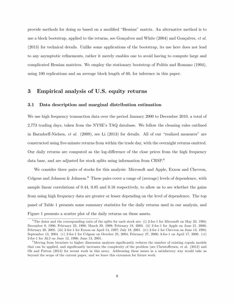
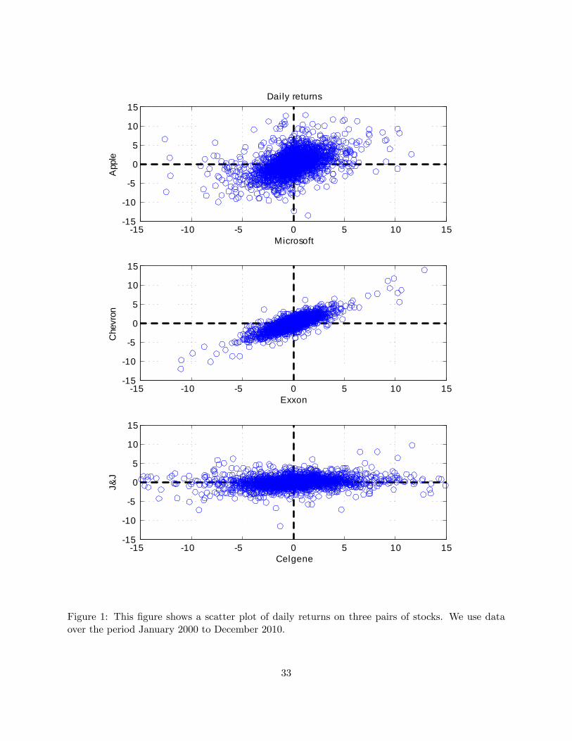
We consider three pairs of stocks for this analysis: Microsoft and Apple, Exxon and Chevron,
Celgene and Johnson & Johnson.9 These pairs cover a range of (average) levels of dependence, with
sample linear correlations of 0.44, 0.85 and 0.16 respectively, to allow us to see whether the gains
from using high frequency data are greater or lesser depending on the level of dependence. The top
panel of Table 1 presents some summary statistics for the daily returns used in our analysis, and
Figure 1 presents a scatter plot of the daily returns on these assets.
8The dates and the corresponding ratio of the splits for each stock are: (i) 2-for-1 for Microsoft on May 23, 1994;December 9, 1996; February 23, 1998; March 29, 1999; February 18, 2003. (ii) 2-for-1 for Apple on June 21, 2000;February 28, 2005. (iii) 2-for-1 for Exxon on April 14, 1997; July 19, 2001. (iv) 2-for-1 for Chevron on June 13, 1994;September 13, 2004. (v) 2-for-1 for Celgene on October 25, 2004; February 27, 2006; 3-for-1 on April 17, 2000. (vi)2-for-1 for J&J on June 12, 1996; June 13, 2001.
9Moving from bivariate to higher dimension analyses signi�cantly reduces the number of existing copula modelsthat can be applied, and signi�cantly increases the complexity of the problem (see Christo¤ersen, et al. (2012) andOh and Patton (2013) for recent work in this area). Addressing these issues in a satisfactory way would take usbeyond the scope of the current paper, and we leave this extension for future work.
8
[ INSERT TABLE 1 AND FIGURE 1 ABOUT HERE ]
As noted in Section 2.3, we use ARMA�GJR-GARCH models to capture the marginal distri-
bution dynamics, with lag lengths chosen using the BIC.10 The second and third panels of Table
1 present the parameter estimates for the conditional mean and variance models. The estimated
parameters are similar to other studies of daily equity returns: generally small AR coe¢ cients,
strongly persistent volatility, with the asymmetric ARCH coe¢ cient being two to four times larger
than the standard ARCH coe¢ cient, indicating asymmetric volatility dynamics.
We use Hansen�s (1994) skewed t for the distribution of the standardized residuals, and the
estimated parameters are presented in the fourth panel of Table 1. The estimated degrees of
freedom parameter, which controls the degree of kurtosis, ranges from 4.5 to 18.8, indicating excess
kurtosis. The skewness parameter, which lies in the interval [�1; 1] for this distribution, is generally
small, indicating evidence of only mild skewness. The bottom panel of Table 1 presents Kolmogorov-
Smirnov and Cramer-von Mises tests of the speci�cation of the marginal distribution. We use a
simulation-based approach to obtain critical values that are correct in the presence of estimated
parameters, see Patton (2013) for details. All of the series pass both of these tests at the 0.05 level,
although there is some mild evidence of misspeci�cation for Apple, and potentially for Exxon. We
proceed with this speci�cation and move on to the estimation of the dynamic copula models.
3.2 High frequency data and dynamic copula models
In Table 2 we present our �rst empirical contribution. This table reports parameters estimates
from three di¤erent GRAS copula models. The �rst is based on a Normal copula, and we model the
arc tan of this parameter evolving according to equation (6). This copula rules out tail dependence
and asymmetric dependence, and is presented as a benchmark model, similar to the DCC model
of Engle (2002). The second is based on a rotated (or survival) Gumbel copula, which allows for
lower tail dependence and asymmetry. The Gumbel copula parameter must lie in [1,1) and we10We consider ARMA(p; q) models up to order (5,5). For four of the six stocks the BIC-optimal model is an
AR(0), i.e., just a constant, while for Exxon the optimal model is an AR(1) and for Chevron an AR(2) is selected.We consider volatility models in the set ARCH(1), ARCH(2), GARCH(1,1), GARCH(2,2), GJR-GARCH(1,1) andGJR-GARCH(2,2). For all six stocks the BIC-optimal model is a GJR-GARCH(1,1) speci�cation.
9

impose this by modeling ' = log (� � 1) : The third model uses a Student�s t copula, which allows
for dependence in both tails, but imposes symmetry. The Student�s t copula has two parameters,
� and ��1; and for simplicity we only allow the correlation parameter � to vary through time.
Like the Normal copula, we model the arc tan of this parameter. In all three models, the GRAS
dynamics are obtained using equation (6), with the realized measure being realized correlation,
computed in the usual way:
RCorrt =RV
(1;2)tq
RV(1;1)t RV
(2;2)t
(9)
where RV (i;j)t =mXk=1
r(i)t;kr
(j)t;k
and m = 78 is the number of �ve-minute returns in a trade day. Our daily returns are whole day
(�close to close�), but we use only open-to-close realized measures in the GRAS models, as this is
the only period of the day in which high frequency data is available.11
The coe¢ cient on lagged realized correlation in the GRAS model is denoted RC ; and is re-
ported in the last row of parameter estimates. Bootstrap standard errors, which take into account
estimation error from the marginal distribution parameters, are presented in parentheses below
the estimated parameters. We see from this table that the coe¢ cient on realized correlation is
signi�cantly di¤erent from zero for all three models across all three pairs of assets. In seven out
of the nine models it is signi�cant at the 1% level, and for the other two it is signi�cant at the
5% level. This is strong statistical evidence of the usefulness of high frequency data for modeling
dynamics in the conditional copula of lower frequency returns, con�rming the general intuition of
Andersen, et al. (2003) for this application.12 ;13
11 In the supplemental appendix we present tables corresponding to Table 2 but using 1-minute, 10-minute and15-minute sampling to obtain realized correlations. The results using 10- and 15-minute sample are similar to thoseusing 5-minute sampling, but worse when using 1-minute sampling, perhaps re�ecting greater market microstructuree¤ects at that frequency.12 In the online supplemental appendix we present a corresponding table of parameter estimates when RC is
imposed to be zero, leading to the GAS speci�cation of Creal, et al. (2012). Comparing the values of the log-likelihoods from that model with those in Table 2 con�rms the gains from including realized correlation in thisspeci�cation.13 In the supplemental appendix we consider all 15 possible pairs out of these six assets, and we present a table of
the p-values from tests comparing the proposed GRAS model to the GAS model. We �nd that 10 out of these 15
10
[ INSERT TABLE 2 ABOUT HERE ]
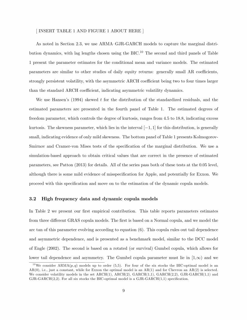
Figure 1 presents the estimated time series of the linear correlation14 from the Student�s t
copula model using the GAS and GRAS speci�cations. (The Student�s t GRAS model beats the
Normal and rotated Gumbel speci�cations for all three pairs of assets, discussed further in Section
3.4 below.) The bottom panel of this �gure, showing the results for Celgene�Johnson & Johnson
is perhaps the easiest to interpret. We see from this �gure that the GRAS model is above to
capture lower and higher values of dependence than the GAS model, which is based only on daily
information. As expected, a model based on higher frequency information is able to adjust to
changes in dependence faster than a model based only on daily information. The same inference
can be made from the other two plots in this �gure, although the parameter dynamics in those
models are such that it is harder to observe.
[ INSERT FIGURE 1 ABOUT HERE ]
3.3 Extensions of the baseline GRAS model
We next consider extensions of the GRAS model presented in equation (6), where we augment that
speci�cation with additional realized measures.
Firstly, we consider an extension motivated by Engle (2002) and Andersen, et al. (2006), who
�nd that conditional correlation is a¤ected by the past level of volatility. We augment our GRAS
speci�cation from above to include not only realized correlation, but also the log realized variance
of each asset. Thus the evolution equation becomes:
't+1 = ! + �'t + �st + RCRCorrt + RV 1 log�RV
(1;1)t
�+ RV 2 log
�RV
(2;2)t
�(10)
The results for this model are presented in Table 3. We again see that the coe¢ cient on lagged
pairs have signi�cant p-values, indicating gains from using the GRAS model. Interestingly, all of the non-signi�cantpairs involve Apple or Microsoft, perhaps indicating that these technology stocks have di¤erent dynamics than theother stocks under consideration.14The linear correlation implied by a copula-based multivariate model is generally not a closed-form function of
the parameters of the model, even when the copula has a �correlation�parameter, see Patton (2013). We use simplenumerical integration to obtain the model-implied linear correlation.
11
realized correlation is highly signi�cant across all models. Further, the coe¢ cients on lagged realized
volatility are signi�cant for two out of three pairs of assets. The last two rows of this table present
joint tests for the signi�cance of the coe¢ cients on realized measures. The penultimate row tests
the restriction that all realized measures have coe¢ cients equal to zero, which simpli�es this model
to a GAS model, and this is strongly rejected. The bottom row tests that only realized correlation
has a non-zero coe¢ cient, and this is strongly rejected for the Microsoft-Apple and Celgene-J&J
pair, but is not rejected for the Exxon-Chevron pair. Thus this table presents evidence that
other measures computed from high frequency data may be helpful in capturing the dynamics of
dependence between asset returns.
[ INSERT TABLE 3 ABOUT HERE ]
Next we consider a �heterogeneous autoregressive�(HAR) version of our baseline model, to see
whether longer-run dependence in realized measures is useful for modeling the dynamics of daily
copulas, see Corsi (2009) and Müller, et al. (1997) for details on the HAR model, and Corsi and
Reno (2009) and Sokolinskiy and van Dijk (2011) for the usefulness of HAR models for forecasting
volatility. Consider the following speci�cation:
't+1 = ! + �'t + �st + RCRCorrt + W1
5
5Xi=1
RCorrt+1�i + M1
22
22Xi=1
RCorrt+1�i (11)
The results for this model are presented in Table 4. We see that the coe¢ cient on lagged
realized correlation is again statistically signi�cant across all nine speci�cations. The coe¢ cients
on the past 5-day and 22-day average realized correlation are generally not signi�cant, indicating
that these additional lags of realized correlation do not much improve the �t of the model (perhaps
due to the persistence that the GAS part of the model already captures). The penultimate row tests
the restriction that all realized measures have coe¢ cients equal to zero, and we are unable to reject
this in any speci�cation, indicating that high frequency information is not useful. This contradicts
our �ndings in the previous section, where high frequency data was found to be strongly signi�cant,
and is explained by the last row of Table 4, where we test the restriction that the coe¢ cients on the
12
weekly and monthly realized correlation lags are zero. We fail to reject this null in all cases, and we
conclude that by including weekly and monthly, as well as daily, realized correlation, we �dilute�
its signi�cance. Overall, it appears that just the one-day lag of realized correlation is useful for
modeling the dynamic copula.
[ INSERT TABLE 4 ABOUT HERE ]
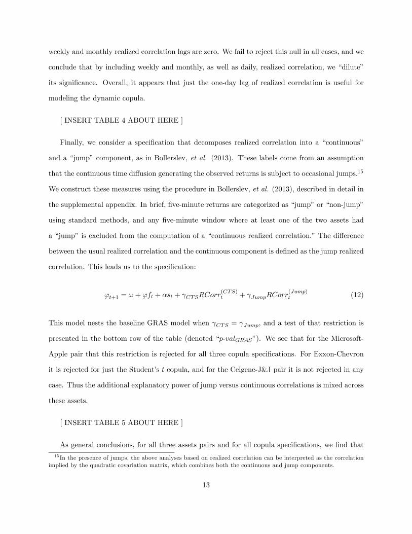
Finally, we consider a speci�cation that decomposes realized correlation into a �continuous�
and a �jump�component, as in Bollerslev, et al. (2013). These labels come from an assumption
that the continuous time di¤usion generating the observed returns is subject to occasional jumps.15
We construct these measures using the procedure in Bollerslev, et al. (2013), described in detail in
the supplemental appendix. In brief, �ve-minute returns are categorized as �jump�or �non-jump�
using standard methods, and any �ve-minute window where at least one of the two assets had
a �jump�is excluded from the computation of a �continuous realized correlation.�The di¤erence
between the usual realized correlation and the continuous component is de�ned as the jump realized
correlation. This leads us to the speci�cation:
't+1 = ! + 'ft + �st + CTSRCorr(CTS)t + JumpRCorr
(Jump)t (12)
This model nests the baseline GRAS model when CTS = Jump; and a test of that restriction is
presented in the bottom row of the table (denoted �p-valGRAS�). We see that for the Microsoft-
Apple pair that this restriction is rejected for all three copula speci�cations. For Exxon-Chevron
it is rejected for just the Student�s t copula, and for the Celgene-J&J pair it is not rejected in any
case. Thus the additional explanatory power of jump versus continuous correlations is mixed across
these assets.
[ INSERT TABLE 5 ABOUT HERE ]
As general conclusions, for all three assets pairs and for all copula speci�cations, we �nd that15 In the presence of jumps, the above analyses based on realized correlation can be interpreted as the correlation
implied by the quadratic covariation matrix, which combines both the continuous and jump components.
13

exploiting information from realized correlation signi�cantly improves the �t of the model. Some
additional explanatory power can be gained for certain assets by also including realized volatilities,
or the continuous and jump components of realized correlations separately, however our baseline
GRAS model, which includes just the one-day lag of realized correlation, generally performs very
well across these assets. In the remainder of the paper we focus on this baseline GRAS speci�cation.
3.4 The choice of copula functional form
Up to this stage of the analysis, we have focused attention on the speci�cation of the dynamics
of the model for the conditional copula (constant, GAS, or GRAS), and paid little attention to
the choice of shape. The estimation results presented above also enable us to shed light on the
best-�tting copula shape across these three pairs of asset returns, and we discuss these results here.
In Table 6 we compare di¤erent speci�cations of the shape of the copula model, holding the
model for the dynamics �xed. The comparison of the rotated Gumbel with the Normal or the
Student�s t involves testing non-nested models, and we use the test of Rivers and Vuong (2002),
see Patton (2013) for a discussion of its implementation for comparing copula models. Given the
models are non-nested, we use a two-sided test for this comparison. The Student�s t copula nests the
Normal copula, and we compare these models via a simple (one-sided) Wald test on the estimated
degrees of freedom parameter.16
The top panel of Table 6 reveals that the rotated Gumbel model generally out-performs the
Normal model, across all three asset pairs and all three models for dynamics, revealed through
the positive t-statistics, however in no case is the di¤erence signi�cant. The lower two panels of
this table reveal the improved �t provided by the Student�s t copula: it signi�cantly beats the
Normal copula in eight out of nine comparisons, and signi�cantly beats the rotated Gumbel in six
out of nine comparisons. This �nding con�rms the importance of allowing for joint fat tails in
multivariate models of asset returns. It is apparent evidence against the importance of allowing for
16Speci�cally, we test that the estimated inverse degrees of freedom parameter is equal to zero. This is on theboundary of the parameter space, which means that the t-statistic will not be standard Normally distributed, howeverthe right-tail critical values, which are the ones we require, remain applicable.
14

asymmetric dependence (e.g., for dependence being higher during market downturns than market
upturns), given that the (symmetric) Student�s t copula outperforms the (asymmetric) rotated
Gumbel copula, however this interpretation is muddied by the additional �exibility the Student�s t
copula attains from it having two free parameters compared with just one for the Gumbel copula.
[ INSERT TABLE 6 ABOUT HERE ]
4 Out-of-sample forecast comparisons
The previous section showed that high frequency data signi�cantly improves the �t of dynamic
copula models for daily asset returns. However, there remains the concern that improved in-
sample �t does not guarantee an improvement in out-of-sample forecast performance. In this
section we investigate whether high frequency information also leads to gains in out-of-sample
forecast performance. We do so using two applications. Firstly, we consider a density forecasting
application, and evaluate performance using a metric related to the Kullback�Leibler information
criterion (KLIC). Secondly, we consider an illustrative portfolio decision problem, and evaluate the
competing models using the realized utility from a portfolio optimized using the predictive density.
4.1 Multivariate density forecasting
We use the approach of Diks et al. (2012), which provides a means of comparing density forecasts
over the entire support, as well as in particular regions of the support. Motivated by its connection
with the Kullback�Leibler information criterion (KLIC), both of these approaches are based on the
out-of-sample log-likelihood of the density forecast. Note that since all of our multivariate models
use the same marginal distribution models (means, variances, and standardized residual densities),
comparing the full multivariate density forecasts from two models reduces to simply comparing the
copula density forecasts.
We use the period from January 2000 to December 2005 as the in-sample period, and January
2006 to December 2010 as our out-of-sample period. Given the computational complexity of the
15

models estimated here, we use a standard rolling window estimation scheme for the marginal
distribution parameters, but a �xed window estimation scheme for the copula parameters.17 In all
cases, the density forecast for day t is based only on information up until day t � 1: Diks et al.
(2012) propose a conditional likelihood test to compare density forecasts, where the performance
of model A in the region [0; q]� [0; q] is based on:
SAt (ut) =�log cAt (ut)� logCAt (q)
�1fut�qg (13)
where q = [q; q]0 and ut = [u1t; u2t]0 : Note that when q = 1 this expression simpli�es to the log
copula density, log cAt (ut) ; and for q < 1 it can be interpreted as the log-likelihood of the model
conditional on the observation lying in the region [0; q]�[0; q]: The null hypothesis of equal predictive
accuracy of models A and B in the region [0; q]� [0; q] is:
H0 : E�SAt (ut)� SBt (ut)
�= 0 (14)
vs. H1 : E�SAt (ut)� SBt (ut)
�6= 0
Diks et al. (2012) propose testing this hypothesis based on a test on the average di¤erence in the
conditional likelihoods. Let:
dt = SAt (ut)� SBt (ut) (15)
then a test that E [dt] = 0 can be used to test the null hypothesis above. This series may be serially
correlated and heteroskedastic, and so robust standard errors are required.18
We consider �ve regions for analysis of the copula density forecasts: the joint 1%, 5% 10% and
25% lower tails, as well as the entire support. The results of these tests are presented in Table
7. The right-most column of this table presents the results for the entire support, and shows that
17The asymptotic testing framework of Giacomini and White (2006), which is used by Diks et al. (2012) toimplement their test, can handle both of these schemes and so this raises no theoretical issues. The out-of-sample�t of the copula models is presumably worse using a �xed window scheme than using a rolling window scheme, butshould not a¤ect our main conclusions on relative performance.18Diks et al. (2012) also propose a �censored likelihood� test as an alternative to the conditional likelihood test.
The results from that test are very similar to those discussed here, and are presented in the supplemental appendix.
16

across all three pairs of assets, and across three copula models (Normal, rotated Gumbel, and
Student�s t) our proposed GRAS model signi�cantly beats the constant copula model in all but one
case. This shows that the dynamics captured by our copula model based on high-frequency data
are useful out-of-sample: the predictive copula densities from the GRAS model provide a better
out-of-sample �t than those from simple, constant parameter copula models. This conclusion holds
true across all joint lower tail regions but one, providing strong support for our model.
A tougher hurdle for our GRAS model is to signi�cantly out-perform the GAS model. The
GAS model provides a parsimonious way of capturing dynamics in the conditional copula, and
our proposed GRAS model will only out-perform it if the high frequency information we exploit
(realized correlation) has additional explanatory power out-of-sample. When looking at the entire
support we �nd that the GRAS beats the GAS model (the t-statistics are positive in 8 out of 9
comparisons), but the out-performance is generally not statistically signi�cant. When we use the
method of Diks et al. (2012) to zoom in on the joint tails of the support, we �nd that the GRAS
model uniformly out-performs the GAS model, and in a majority of comparisons the di¤erence is
statistically signi�cant. Thus it appears that high frequency information is particularly useful for
dynamic copula models when interest is focused on the tails of the distribution.
[ INSERT TABLE 7 ABOUT HERE ]
4.2 A portfolio decision problem
Previous work has documented evidence of two types of asymmetries in the joint distribution of
stock returns, namely skewness in the distribution of individual returns, and asymmetry in the
dependence between asset returns.19 With this motivation, we use a portfolio application to gain
insights into the economic signi�cance of using high frequency data in dynamic copula models. We
approach the portfolio allocation problem following the methodology proposed in Patton (2004)
and Jondeau and Rockinger (2012). The latter paper proposes approximating a CRRA utility
19See Erb, et al. (1994), Longin and Solnik (2001), Ang and Chen (2002), and Patton (2004) for example.
17
function using a fourth-order polynomial for tractability:
Et [U (Wt+1)] = '0 + '1m(1)t+1 + '2m
(2)t+1 + '3m
(3)t+1 + '4m
(4)t+1 (16)
with 'k = (k!)�1 @kU (W ) =dW kjW=1; which are known functions of k and the degree of risk
aversion, and m(j)t+1 = Et
hW jt+1
iis the uncentered jth moment, withWt+1 the value of the portfolio
at time t + 1:20 We consider �ve di¤erent levels of relative risk aversion, RRA = 1; 3; 7; 10 and
20, similar to the range considered in Campbell and Viceira (1999) and Aït-Sahalia and Brandt
(2001).
Optimal portfolio weights are found by maximizing the expected utility under the predictive
density:
!�t+1 = argmax!2�
Et�U�1 + !0Yt+1
��(17)
= argmax!2�
Z ZU (1 + !1y1 + !2y2) f̂1;t+1 (y1) f̂2;t+1 (y2)bct+1 �F̂1;t+1 (y1) ; F̂2;t+1 (y2)� dy1dy2
where � is a compact subset of R2 for the unconstrained investor, and the two-dimensional unit
simplex21 for the short-sales constrained investor. For simplicity we take the return on the risk-free
asset to be zero.
We use the same in-sample and out-of-sample periods as in the previous section, but in this
section we evaluate the competing models using the average utility of the portfolio returns formed
using weights optimized according to the model. To make the units used in this performance study
interpretable, we convert the average utility into a �management fee,�which is the �xed amount,
#; that could be charged (or paid, if needed) each period to an investor to switch from model A
to model B. Alternatively, it can be interpreted as the amount that could be deducted from the
daily return on portfolio B over the out-of-sample period and leave the investor indi¤erent between20The optimal portfolio weights under a CRRA utility function do not depend on the level of initial wealth, and
so we set the initial wealth to 1. Thus the end-of-period wealth is equal to the gross return on the portfolio.
21That is, for short sales constrained investors, � =�(!1; !2) 2 [0; 1]2 : !1 + !2 � 1
:
18
portfolio A and portfolio B. The management fee is the solution to the following equation:
1
P
R+PXt=R+1
U�1 + !�0A;t+1Yt+1
�=1
P
R+PXt=R+1
U�1 + !�0B;t+1Yt+1 � #
�(18)
where R is the length of the in-sample period and P is the length of the out-of-sample period.
Table 8 presents the management fees estimates, and for all comparisons we consider switching
from a smaller model (Constant or GAS) to the larger model (GRAS).22 ;23 Consider �rst the
comparison of the constant copula model and the GRAS model. Across all asset pairs, copula
shape speci�cations, and levels of risk aversion, we see that the GRAS model is generally preferred:
the management fees are positive in a majority of cases, and are signi�cantly positive for two of
the asset pairs (Microsoft-Apple and Celgene-J&J) when combined with the Student�s t copula.
For example, for the Microsoft-Apple pair, the annualized management fees that could be charged
to switch from a constant t copula to a GRAS t copula range from 43.0% (RRA=1) to 1.3%
(RRA=20), and is 4.0% for the intermediate level of risk aversion.24 In no case is the management
fee negative and signi�cant. This is strong out-of-sample support for our GRAS model, at least
against the simple benchmark of a constant copula.
As in the previous section, a tougher benchmark for the GRAS model is the GAS speci�cation.
In this case the results are more mixed: for Celgene-J&J we �nd that the GRAS copula is preferred
to the GAS copula, particularly when combined with the Student�s t shape speci�cation. For Exxon-
Chevron, the GRAS model is generally preferred, with the performance fees ranging from -1.9%
to +17.9%, but these are not statistically signi�cant in any case, indicating that the GAS and
GRAS models are equally good out-of-sample, according to this metric. For the Microsoft-Apple
22The supplemental appendix presents some summary statistics on the portfolio returns, as well as results forthe short-sales constrained investor, which yields conclusions that are consistent with those for the unconstrainedinvestor. The supplemental appendix also presents plots the optimal portfolio weights for some representative models.For lower levels of risk aversion, these plots reveal substantial portfolio turnover, and in practice it may be desirableto impose turnover constraints on the optimization problem. We do not attempt this here.23We use a stationary bootstrap with average block length of 60 days to determine the signi�cance of the �man-
agement fees.� Note that the quantities being bootstrapped here are asset returns, not cumulative wealth, and soissues of non-stationarity or integrated processes do not arise.24 In almost all cases, we �nd that the absolute value of the management fee decreases with the level of risk aversion.
This re�ects the fact that more risk averse investors shrink their weights on risky assets towards zero, making thedi¤erences in portfolio weights from di¤erent models smaller.
19
pair the GRAS model is beaten by the GAS model, with the performance fees being negative
and often signi�cant. Thus the out-of-sample gains from a GRAS model relative to a GAS model
from a portfolio decision perspective are somewhat sensitive to the choice of assets and the copula
shape speci�cation: in some cases positive and signi�cant, in others negative and signi�cant, and
in yet others not di¤erent from zero. Further work on the determinants of this variability is clearly
desirable, as is a more comprehensive and higher-dimension portfolio decision application.
[ INSERT TABLE 8 ABOUT HERE ]
5 Conclusion
This paper proposes a new class of dynamic copula models for daily asset returns that exploits
information from high frequency (intra-daily) data. This class of models bridges the gap between
the existing time-varying copula models, which have almost exclusively used lower frequency data,
and models from the volatility and correlation forecasting literature, which have successfully used
high frequency data. We accomplish this by augmenting the generalized autoregressive score (GAS)
model of Creal, et al. (2013) with high frequency measures, such as realized correlation, to ob-
tain a �realized GAS,� (GRAS) model. While measures of dependence based in high frequency
data cannot generally be interpreted as unbiased or consistent estimators of dependence and lower
frequencies, our approach builds on the intuition that by better measuring the current degree of
dependence, broadly de�ned, we can build better forecasts of dependence in the future.
We employ equity return data six U.S. �rms over the period 2000 to 2010, and show that
including high frequency information in a dynamic model of daily equity return dependence leads
to improvements in both goodness of �t and out-of-sample forecasts. In sample, we �nd that the
information in realized correlation leads to signi�cant improvements across all assets and copula
speci�cations considered, and we �nd some evidence that realized volatility, and a measure of
correlation that is related to �co-jumps,�improves our baseline GRAS model even more for certain
assets. Out of sample, we �nd that density forecasts based on our GRAS speci�cation outperform
20

forecasts based on models that ignore high frequency information, and this outperformance is
strongly signi�cant when attention is focused on the tail of the joint distribution. We also �nd
some gains in out-of-sample portfolio construction based on these density forecasts, though the
gains vary across the assets under consideration.
While this paper provides some initial light on the value of high frequency information for
lower frequency copula modeling, some important questions remain open. Firstly, it would be
interesting extend the analysis in this paper to high dimension copula models, along the lines of
Christo¤ersen, et al. (2012) and Oh and Patton (2013) for example. Estimates of large-dimension
realized covariance matrices have recently attracted attention, see Hautsch et al. (2012) for example,
and these could prove useful in an extension of GRAS models to high dimensions. Furthermore,
extending and elaborating the portfolio decision application presented above would enable a better
understanding of the economic value of high frequency information for dynamic copula modeling.
We leave these important extensions for future research.
References
[1] Aït-Sahalia, Y., and M.W. Brandt., 2001, "Variable Selection for Portfolio Choice," Journalof Finance 56, 1297�1355.
[2] Andersen T.G., T. Bollerslev, P.F. Christo¤ersen and F.X. Diebold, 2006, "Volatility andCorrelation Forecasting", in Handbook of Economic Forecasting (eds. Graham Elliott, CliveW.J. Granger and Allan Timmermann), Elsevier Science B.V., Amsterdam.
[3] Andersen T.G., T. Bollerslev and F.X. Diebold, 2013, "Financial Risk Measurement for Fi-nancial Risk Management", Handbook of the Economics of Finance, 2, 1127-1220.
[4] Andersen, T.G., T. Bollerslev and P. Labys, 2003, �Modeling and Forecasting Realized Volatil-ity�, Econometrica, 71, 3�29.
[5] Ang, A., and J. Chen, 2002, "Asymmetric Correlations of Equity Portfolios", Journal of Fi-nancial Economics, 63, 443�494.
[6] Barndor¤-Nielsen, O. E., P.R. Hansen, A. Lunde and N. Shephard, 2009, "Realized kernels inpractice: trades and quotes", Econometrics Journal, 12, 1�32.
[7] Barndor¤-Nielsen, O. E. and N. Shephard, 2007, "Variation, jumps, market frictions and highfrequency data in nancial econometrics," In R. Blundell, P. Torsten, and W.K. Newey, edi-tors, Advances in economics and econometrics. Theory and applications, Econometric SocietyMonographs, 328-372. Cambridge University Press, Cambridge.
21
[8] Blasques, F., S.J. Koopman and A. Lucas, 2012, Stationarity and Ergodicity of UnivariateGeneralized Autoregressive Score Processes, Tinbergen Institute Discussion Paper TI 2012-059/4.
[9] Bollerslev, T., 1986, "Generalized autoregressive conditional heteroskedasticity," Journal ofEconometrics, 31, 307-327.
[10] Bollerslev, T., 2009, "Glossary to ARCH (GARCH)", in Volatility and Time Series Economet-rics: Essays in Honor of Robert F. Engle (eds. Tim Bollerslev, Je¤rey R. Russell and MarkW. Watson), Oxford University Press, Oxford.
[11] Bollerslev T., S.Z. Li and V. Todorov, 2013, "Jump Tails, Extreme Dependencies and theDistribution of Stock Returns", Journal of Econometrics, 172, 307�324.
[12] Campbell, J.Y., and L.M. Viceira, 1999, "Consumption and Portfolio Decisions When Ex-pected Returns are Time Varying,�Quarterly Journal of Economics, 114, 433�495.
[13] Christo¤ersen, P., V.R. Errunza, K. Jacobs and H. Langlois, 2012, "Is the Potential for In-ternational Diversi�cation Disappearing? A Dynamic Copula Approach", Review of FinancialStudies, 25, 3711-3751.
[14] Corsi, F., 2009, "A simple approximate long-memory model of realized volatility," Journal ofFinancial Econometrics, 7, 174-196.
[15] Corsi F., D. Pirino and R. Reno, 2011, "HAR Modeling for Realized Volatility Forecasting",Handbook in Financial Engineering and Econometrics: Volatility Models and Their Applica-tions, forthcoming.
[16] Creal, D., S. J. Koopman, and A. Lucas, 2013, "Generalized autoregressive score models withapplications", Journal of Applied Econometrics, 28, 777�795.
[17] Davis, R.A., W.T.M. Dunsmuir, and S. Streett, 2003, "Observation driven models for Poissoncounts," Biometrika, 90, 777�790.
[18] Diks C., V. Panchenko, O. Sokolinskiy, and D. van Dijk, 2012, "Comparing the Accuracy ofCopula-Based Multivariate Density Forecasts in Selected Regions of Support", working paper.
[19] Engle, R.F., 1982, "Autoregressive Conditional Heteroscedasticity with Estimates of the Vari-ance of UK In�ation," Econometrica, 50, 987-1007.
[20] Engle, R. F., 2002, "Dynamic Conditional Correlation: A Simple Class of Multivariate Gener-alized Autoregressive Conditional Heteroskedasticity Models", Journal of Business and Eco-nomic Statistics, 20, 339-350.
[21] Engle, R.F. and J.R. Russell, 1998, "Autoregressive Conditional Duration: A New Model forIrregularly Spaced Transaction Data," Econometrica, 66, 1127-1162.
[22] Erb, C.B., C.R. Harvey, and T.E. Viskanta, 1994, "Forecasting International Equity Correla-tions", Financial Analysts Journal, 50, 32�45.
[23] Fengler, M.R. and O. Okhrin, 2012, "Realized Copula", SFB 649 Discussion Papers.
22

[24] Giacomini, R. and H. White, 2006, "Tests of conditional predictive ability", Econometrica, 74,1545�1578
[25] Glosten, L.R., R. Jagannathan and D.E. Runkle, 1993, "On the Relation between the ExpectedValue and the Volatility of the Nominal Excess Return on Stocks", Journal of Finance, 48,1779-1801.
[26] Gonçalves, S. and H. White, 2004, "Maximum likelihood and the bootstrap for nonlineardynamic models", Journal of Econometrics, 119, 199-219.
[27] Gonçalves, S., U. Hounyo, A.J. Patton and K. Sheppard, 2013, "Bootstrapping two-stageextremum estimators", working paper, Oxford-Man Institute of Quantitative Finance.
[28] Hafner, C.M. and H. Manner, 2011, "Dynamic Stochastic Copula Models: Estimation, Infer-ence and Applications," Journal of Applied Econometrics, forthcoming.
[29] Han, H., 2013, Asymptotic Properties of GARCH-X Processes, Journal of Financial Econo-metrics, forthcoming.
[30] Hansen, B.E., 1994, "Autoregressive conditional density estimation", International EconomicReview, 35, 705-730.
[31] Hansen P.R., Z. Huang and H. H. Shek, 2011, "Realized GARCH: A Joint Model for Returnsand Realized Measures of Volatility", Journal of Applied Econometrics, 27, 877-906.
[32] Hansen P.R., A. Lunde and V. Voev, 2013, "Realized Beta GARCH: A Multivariate GARCHModel with Realized Measures of Volatility", Journal of Applied Econometrics, forthcoming.
[33] Harvey, A.C., 2013, Dynamic Models for Volatility and Heavy Tails, Econometric SocietyMonograph 52, Cambridge University Press, Cambridge.
[34] Harvey, A.C. and G. Sucarrat, 2012, "EGARCH models with fat tails, skewness and leverage,"Computational Statistics and Data Analysis, forthcoming.
[35] Hautsch, N., L.M. Kyj and R.C.A. Oomen, 2012, "A blocking and regularization approachto high dimensional realized covariance estimation," Journal of Applied Econometrics, 27,625-645.
[36] Joe, H., 2005, Asymptotic e¢ ciency of the two-stage estimation method for copula-basedmodels, Journal of Multivariate Analysis, 94, 401-419.
[37] Jondeau, E. and M. Rockinger, 2006, "The copula-GARCH model of conditional dependencies:An international stock market application," Journal of International Money and Finance, 25,827�853.
[38] Jondeau E. and M. Rockinger, 2012, "On the Importance of Time Variability in Higher Mo-ments for Asset Allocation", Journal of Financial Econometrics, 10, 84-123.
[39] Li, S. Z., 2013, "Continuous Beta, Discontinuous Beta, and the Cross-Section of ExpectedStock Returns," working paper, Department of Economics, Duke University.
23

[40] Longin, F., and B. Solnik, 2001, "Extreme Correlation of International Equity Markets",Journal of Finance, 56, 649�676.
[41] Müller U., M., R. D. Dacorogna, R. Olsen, O. Pictet and J. Von Weizsacker, 1997, �Volatili-ties of di¤erent time resolutions -analysing the dynamics of market components�, Journal ofEmpirical Finance, 4, 213�39.
[42] Noureldin D., N. Shephard and K. Sheppard, 2012, "Multivariate high-frequency-based volatil-ity (HEAVY) models", Journal of Applied Econometrics, 27, 907-933
[43] Oh, D.-H. and A.J. Patton, 2013, "Modelling Dependence in High Dimensions using FactorCopulas", working paper, Duke University.
[44] Okimoto, T., 2008, "New evidence of asymmetric dependence structure in international equitymarkets," Journal of Financial and Quantitative Analysis, 43, 787�815.
[45] Patton A.J., 2004, "On the Out-of-Sample Importance of Skewness and Asymmetric Depen-dence for Asset Allocation", Journal of Financial Econometrics, 2, 130-168.
[46] Patton A.J., 2006a, "Modelling Asymmetric Exchange Rate Dependence", International Eco-nomic Review, 47, 527-556.
[47] Patton A.J., 2006b, "Estimation of Multivariate Models for Time Series of Possibly Di¤erentLengths", Journal of Applied Econometrics, 21, 147-173.
[48] Patton, A.J., 2013, Copula methods for forecasting multivariate time series, in G. Elliott andA. Timmermann (eds.), Handbook of Economic Forecasting, Volume 2, Elsevier, Oxford.
[49] Politis, D.N., and J.P. Romano, 1994, The Stationary Bootstrap, Journal of the AmericanStatistical Association, 89, 1303-1313.
[50] Rivers, D. and Q. Vuong, 2002, "Model Selection Tests for Nonlinear Dynamic Models," Econo-metrics Journal, 5, 1-39.
[51] Rodriguez, J.C., 2007, "Measuring �nancial contagion: a copula approach," Journal of Empir-ical Finance, 14(3), 401-423.
[52] Shephard N. and K. Sheppard, 2010, "Realising the future: forecasting with high frequencybased volatility (HEAVY) models", Journal of Applied Econometrics, 25, 197-231.
[53] Sklar, A., 1959, "Fonctions de répartition à n dimensions et leurs marges", Publications del�Institut Statistique de l�Universite´ de Paris, 8, 229-231.
[54] Sokolinskiy O. and D. van Dijk, 2011, "Forecasting Volatility with Copula-Based Time SeriesModels", Tinbergen Institute Discussion Paper.
[55] White, H., 1994, "Estimation, Inference and Speci�cation Analysis, Econometric SocietyMonographs No. 22, Cambridge University Press, Cambridge, U.K.
24

Table 1: Summary statistics and marginal distribution estimates
Microsoft Apple Exxon Chevron Celgene J&J
Panel A: Summary statisticsMean -0.027 0.119 0.022 0.028 0.085 0.010Std dev 2.209 2.958 1.745 1.770 3.618 1.374Skewness -0.083 -0.138 0.178 0.158 -0.140 -0.788Kurtosis 11.221 6.390 14.374 14.230 8.714 18.733
Correl (linear/rank) 0.437/0.478 0.851/0.803 0.163/0.218
Panel B: Conditional meanConstant -0.027 0.119 0.026 0.034 0.085 0.010AR(1) -0.138 -0.118AR(2) -0.079
Panel C: Conditional varianceConstant 0.079 0.106 0.057 0.068 0.059 0.020ARCH 0.041 0.026 0.029 0.025 0.014 0.031
Asym ARCH 0.074 0.050 0.076 0.088 0.032 0.110GARCH 0.906 0.937 0.907 0.900 0.964 0.905
Panel D: Skew t densityDoF 4.498 5.977 9.464 18.768 5.027 5.881Skew -0.008 0.031 -0.125 -0.109 0.017 -0.020
Panel E: GoF testsKS p-value 0.708 0.088 0.066 0.380 0.543 0.785CvM p-value 0.507 0.059 0.109 0.315 0.588 0.842
Notes: The top panel of this table presents summary statistics on the daily returns for six U.S. �rms,listed in the column headings. The second panel presents the parameter estimates for AR(p) models of theconditional means of these returns, and the third panel presents parameter estimates for GJR-GARCH(1,1)models of the conditional variance. The fourth panel presents parameter estimates for Hansen�s (1994)skew t density for the standardized residuals. The bottom panel presents simulation-based p-values fromKolmogorov-Smirnov and Cramer-von Mises tests of the goodness-of-�t of the density speci�cation.
25
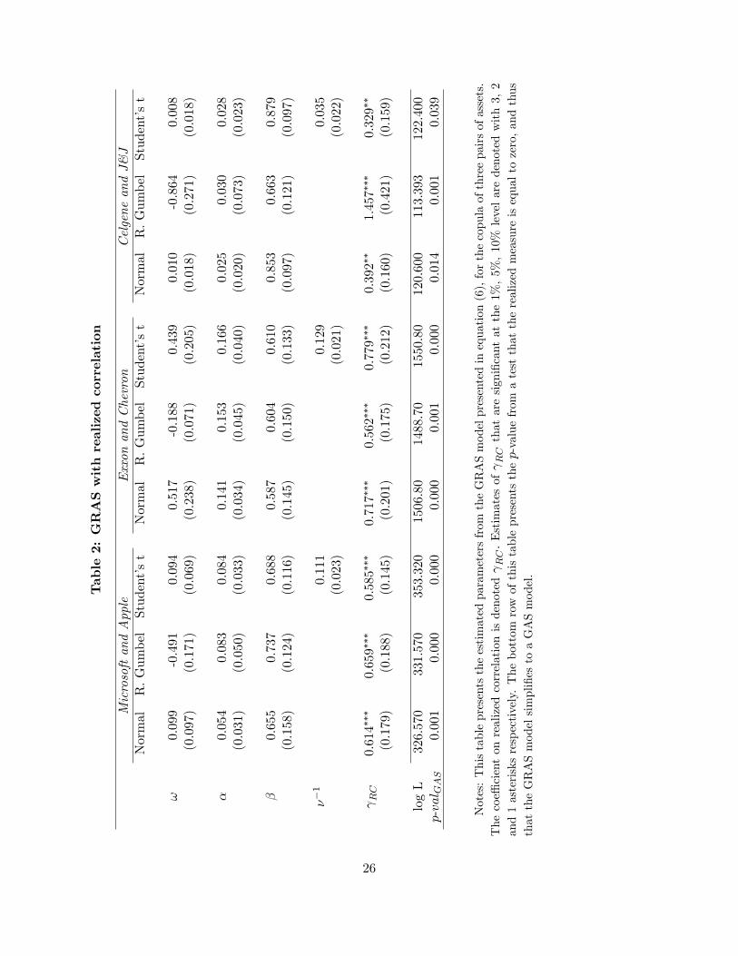
Table2:GRASwithrealized
correlation
MicrosoftandApple
ExxonandChevron
CelgeneandJ&J
Normal
R.Gumbel
Student�st
Normal
R.Gumbel
Student�st
Normal
R.Gumbel
Student�st
!0.099
-0.491
0.094
0.517
-0.188
0.439
0.010
-0.864
0.008
(0.097)
(0.171)
(0.069)
(0.238)
(0.071)
(0.205)
(0.018)
(0.271)
(0.018)
�0.054
0.083
0.084
0.141
0.153
0.166
0.025
0.030
0.028
(0.031)
(0.050)
(0.033)
(0.034)
(0.045)
(0.040)
(0.020)
(0.073)
(0.023)
�0.655
0.737
0.688
0.587
0.604
0.610
0.853
0.663
0.879
(0.158)
(0.124)
(0.116)
(0.145)
(0.150)
(0.133)
(0.097)
(0.121)
(0.097)
��1
0.111
0.129
0.035
(0.023)
(0.021)
(0.022)
RC
0.614���
0.659���
0.585���
0.717���
0.562���
0.779���
0.392��
1.457���
0.329��
(0.179)
(0.188)
(0.145)
(0.201)
(0.175)
(0.212)
(0.160)
(0.421)
(0.159)
logL
326.570
331.570
353.320
1506.80
1488.70
1550.80
120.600
113.393
122.400
p-val GAS
0.001
0.000
0.000
0.000
0.001
0.000
0.014
0.001
0.039
Notes:Thistablepresentstheestimatedparametersfrom
theGRASmodelpresentedinequation(6),forthecopulaofthreepairsofassets.
Thecoe¢cientonrealizedcorrelationisdenoted RC:Estimatesof RCthataresigni�cantatthe1%,5%,10%levelaredenotedwith3,2
and1asterisksrespectively.Thebottomrowofthistablepresentsthep-valuefrom
atestthattherealizedmeasureisequaltozero,andthus
thattheGRASmodelsimpli�estoaGASmodel.
26

Table3:GRASwithrealized
correlationandrealized
variance
MicrosoftandApple
ExxonandChevron
CelgeneandJ&J
Normal
R.Gumbel
Student�st
Normal
R.Gumbel
Student�st
Normal
R.Gumbel
Student�st
!0.085
-0.812
0.121
0.483
-0.364
0.395
-0.540
-3.254
-0.507
(0.161)
(0.477)
(0.164)
(0.364)
(0.496)
(0.374)
(0.405)
(0.960)
(0.426)
�0.053
0.080
0.078
0.148
0.156
0.171
-0.018
-0.046
-0.010
(0.036)
(0.066)
(0.037)
(0.032)
(0.041)
(0.041)
(0.033)
(0.097)
(0.035)
�0.657
0.671
0.688
0.549
0.570
0.589
0.177
0.257
0.191
(0.200)
(0.130)
(0.114)
(0.167)
(0.157)
(0.150)
(0.185)
(0.137)
(0.175)
��1
0.109
0.130
0.025
(0.020)
(0.020)
(0.023)
RC
0.528��
0.746���
0.500���
0.851���
0.641���
0.869���
0.945���
1.810���
0.924���
(0.221)
(0.256)
(0.180)
(0.278)
(0.216)
(0.267)
(0.181)
(0.347)
(0.188)
RV1
0.055�
0.055�
0.053��
0.122��
0.038
0.070�
-0.247���
-0.467���
-0.245���
(0.031)
(0.033)
(0.025)
(0.055)
(0.058)
(0.039)
(0.066)
(0.101)
(0.057)
RV2
-0.066�
-0.091��
-0.059��
-0.127�
-0.054
-0.075
0.107��
0.199��
0.110��
(0.039)
(0.042)
(0.027)
(0.067)
(0.071)
(0.061)
(0.050)
(0.090)
(0.047)
logL
330.565
336.124
355.494
1509.90
1489.30
1551.70
131.080
126.280
132.020
p-val GAS
0.010
0.010
0.000
0.000
0.000
0.000
0.000
0.000
0.000
p-val GRAS
0.050
0.020
0.000
0.050
0.500
0.220
0.000
0.000
0.000
Notes:Thistablepresentstheestimatedparametersfrom
theGRASmodelpresentedinequation(6),forthecopulaofthree
pairsofassets.Thecoe¢cientonrealizedcorrelationisdenoted RC:Estimatesof RC; RV1;or RV2thataresigni�cantatthe
1%,5%,10%levelaredenotedwith3,2and1asterisksrespectively.Thepenultimaterowofthistablepresentsthep-valuefrom
atestthatallcoe¢cientsonrealizedmeasuresareequaltozero.Thebottomrowpresentsthep-valuefrom
atestthatallcoe¢cients
onrealizedmeasuresexceptforthatonthelaggedrealizedcorrelationareequaltozero.
27

Table4:GRASwithHARrealized
correlations
MicrosoftandApple
ExxonandChevron
CelgeneandJ&J
Normal
R.Gumbel
Student�st
Normal
R.Gumbel
Student�st
Normal
R.Gumbel
Student�st
!0.037
-0.748
0.054
0.535
-0.249
0.475
0.002
-0.026
0.002
(0.089)
(0.417)
(0.079)
(0.250)
(0.153)
(0.214)
(0.048)
(0.947)
(0.046)
�0.059
0.097
0.089
0.153
0.168
0.183
0.023
0.046
0.023
(0.038)
(0.068)
(0.036)
(0.030)
(0.037)
(0.040)
(0.033)
(0.097)
(0.032)
�0.570
0.628
0.643
0.553
0.538
0.540
0.968
0.990
0.970
(0.234)
(0.211)
(0.175)
(0.182)
(0.235)
(0.179)
(0.322)
(0.366)
(0.319)
��1
0.110
0.127
0.036
(0.021)
(0.019)
(0.021)
RC
0.569��
0.646�
0.582���
0.536��
0.361�
0.524���
0.463���
0.821�
0.440��
(0.254)
(0.357)
(0.214)
(0.268)
(0.217)
(0.225)
(0.181)
(0.485)
(0.189)
W
-0.313
-0.112
-0.268
-0.517
-0.227
-0.366
-0.410
-0.724
-0.386
(0.550)
(0.589)
(0.463)
(0.571)
(0.523)
(0.500)
(0.547)
(0.829)
(0.519)
M
0.734
0.533
0.507
0.805�
0.572
0.836�
0.035
-0.047
0.030
(0.644)
(0.696)
(0.555)
(0.448)
(0.494)
(0.463)
(0.659)
(1.270)
(0.709)
logL
329.189
332.347
354.534
1510.10
1491.20
1553.20
121.710
117.400
123.470
p-val GAS
0.270
0.480
0.360
0.260
0.370
0.230
0.840
0.670
0.860
p-val GRAS
0.310
0.580
0.410
0.280
0.410
0.240
0.870
0.770
0.860
Notes:Thistablepresentstheestimatedparametersfrom
theGRASmodelpresentedinequation(6),forthecopulaofthree
pairsofassets.Thecoe¢cientonrealizedcorrelationisdenoted RC:Estimatesof RC; W;or Mthataresigni�cantatthe1%,
5%,10%levelaredenotedwith3,2and1asterisksrespectively.Thepenultimaterowofthistablepresentsthep-valuefrom
atest
thatallcoe¢cientsonrealizedmeasuresareequaltozero.Thebottomrowpresentsthep-valuefrom
atestthatallcoe¢cientson
realizedmeasuresexceptforthatonthelaggedrealizedcorrelationareequaltozero.
28
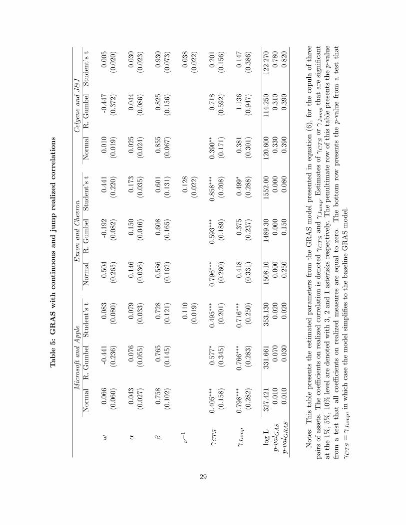
Table5:GRASwithcontinuousandjumprealized
correlations
MicrosoftandApple
ExxonandChevron
CelgeneandJ&J
Normal
R.Gumbel
Student�st
Normal
R.Gumbel
Student�st
Normal
R.Gumbel
Student�st
!0.066
-0.441
0.083
0.504
-0.192
0.441
0.010
-0.447
0.005
(0.060)
(0.236)
(0.080)
(0.265)
(0.082)
(0.220)
(0.019)
(0.372)
(0.020)
�0.043
0.076
0.079
0.146
0.150
0.173
0.025
0.044
0.030
(0.027)
(0.055)
(0.033)
(0.036)
(0.046)
(0.035)
(0.024)
(0.086)
(0.023)
�0.758
0.765
0.728
0.586
0.608
0.601
0.855
0.825
0.930
(0.102)
(0.145)
(0.121)
(0.162)
(0.165)
(0.131)
(0.067)
(0.156)
(0.073)
��1
0.110
0.128
0.038
(0.019)
(0.022)
(0.022)
CTS
0.405���
0.577�
0.495���
0.796���
0.593���
0.858���
0.390��
0.718
0.201
(0.158)
(0.345)
(0.201)
(0.260)
(0.189)
(0.208)
(0.171)
(0.592)
(0.156)
Jump
0.798���
0.766���
0.716���
0.418
0.375
0.499�
0.381
1.136
0.147
(0.282)
(0.283)
(0.250)
(0.331)
(0.237)
(0.288)
(0.301)
(0.947)
(0.386)
logL
327.421
331.661
353.130
1508.10
1489.30
1552.00
120.600
114.250
122.270
p-val GAS
0.010
0.070
0.020
0.000
0.000
0.000
0.330
0.310
0.780
p-val GRAS
0.010
0.030
0.020
0.250
0.150
0.080
0.390
0.390
0.820
Notes:Thistablepresentstheestimatedparametersfrom
theGRASmodelpresentedinequation(6),forthecopulaofthree
pairsofassets.Thecoe¢cientsonrealizedcorrelationisdenoted CTSand Jump:Estimatesof CTSor Jumpthataresigni�cant
atthe1%,5%,10%levelaredenotedwith3,2and1asterisksrespectively.Thepenultimaterowofthistablepresentsthep-value
from
atestthatallcoe¢cientsonrealizedmeasuresareequaltozero.Thebottomrowpresentsthep-valuefrom
atestthat
CTS= Jump;inwhichcasethemodelsimpli�estothebaselineGRASmodel.
29
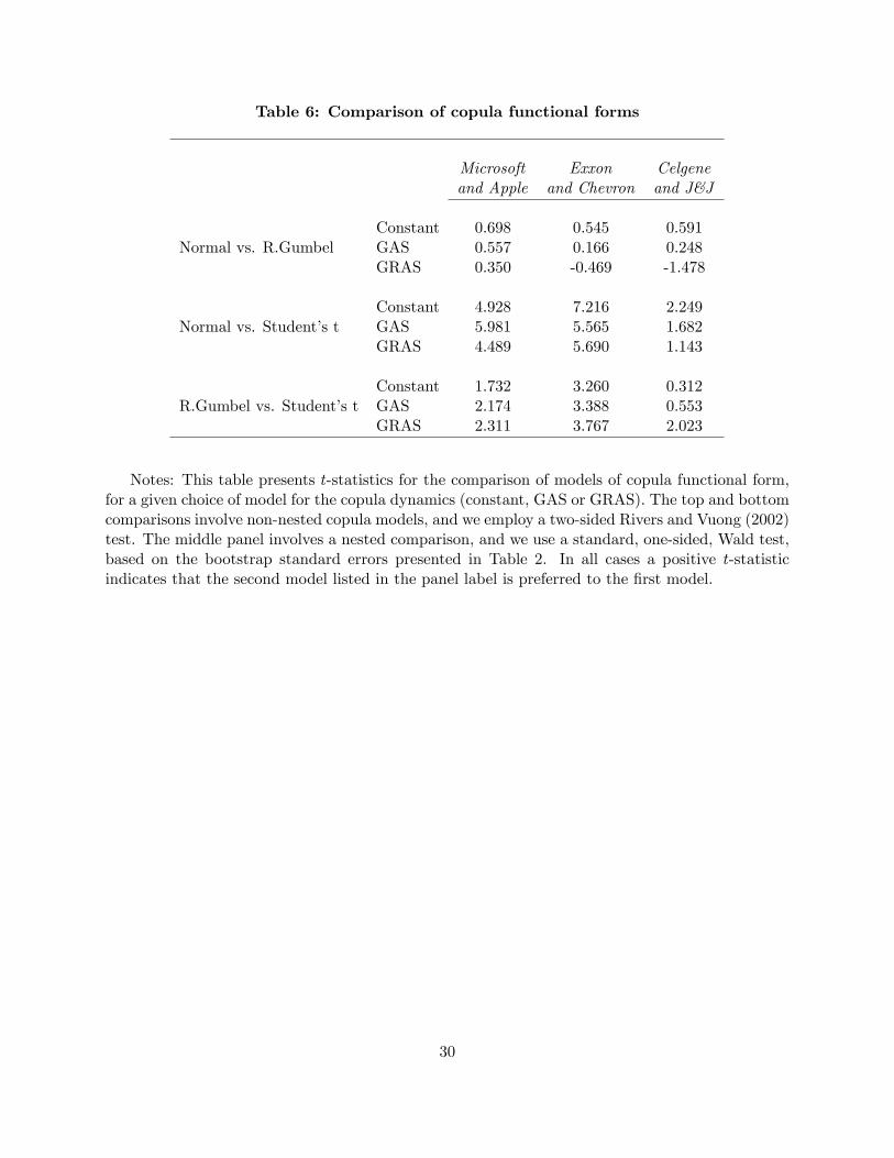
Table 6: Comparison of copula functional forms
Microsoft Exxon Celgeneand Apple and Chevron and J&J
Constant 0.698 0.545 0.591Normal vs. R.Gumbel GAS 0.557 0.166 0.248
GRAS 0.350 -0.469 -1.478
Constant 4.928 7.216 2.249Normal vs. Student�s t GAS 5.981 5.565 1.682
GRAS 4.489 5.690 1.143
Constant 1.732 3.260 0.312R.Gumbel vs. Student�s t GAS 2.174 3.388 0.553
GRAS 2.311 3.767 2.023
Notes: This table presents t-statistics for the comparison of models of copula functional form,for a given choice of model for the copula dynamics (constant, GAS or GRAS). The top and bottomcomparisons involve non-nested copula models, and we employ a two-sided Rivers and Vuong (2002)test. The middle panel involves a nested comparison, and we use a standard, one-sided, Wald test,based on the bootstrap standard errors presented in Table 2. In all cases a positive t-statisticindicates that the second model listed in the panel label is preferred to the �rst model.
30

Table 7: Out-of-sample comparison of density forecasts
Lower tail region probability0.01 0.05 0.10 0.25 1.00
Microsoft and AppleNormal 1.338� 2.126�� 3.232��� 3.142��� 1.536�
GRAS vs. Const R. Gumbel 1.291� 1.799�� 2.974��� 3.279��� 2.000��
Student�s t 1.724�� 1.923�� 3.242��� 3.149��� 2.014��
Normal 1.100 1.471� 2.790��� 3.164��� 1.192GRAS vs. GAS R. Gumbel 0.855 0.980 2.086�� 2.472��� 0.997
Student�s t 1.703�� 0.948 2.303�� 2.601��� 0.932
Exxon and ChevronNormal 2.649��� 6.363��� 7.845��� 8.857��� 2.770���
GRAS vs. Const R. Gumbel 0.871 3.819��� 3.523��� 3.678��� 3.530���
Student�s t 2.598��� 6.174��� 7.387��� 8.934��� 3.236���
Normal 2.624��� 6.120��� 7.312��� 7.725��� 1.081GRAS vs. GAS R. Gumbel 0.132 2.546��� 1.538� 1.143 1.475�
Student�s t 2.297�� 5.562��� 6.240��� 7.033��� 1.618�
Celgene and J&JNormal 1.328� 3.130��� 4.520��� 8.260��� 3.100���
GRAS vs. Const R. Gumbel 1.287� 2.982��� 4.191��� 7.302��� 1.240Student�s t 1.300� 3.123��� 4.524��� 8.308��� 2.586���
Normal 1.384� 2.894��� 3.999��� 7.153��� 0.623GRAS vs. GAS R. Gumbel 1.397� 2.912��� 4.107��� 6.584��� -0.375
Student�s t 1.405� 2.912��� 4.084��� 7.203��� 0.138
Notes: This table presents t-statistics from pair-wise comparisons of the out-of-sample likeli-hoods of competing density forecasts. We consider �ve regions of support over which to comparethe competing density forecasts: the joint lower 0.01, 0.05, 0.10 and 0.25 tails, as well as the entiresupport. For a given copula speci�cation (Normal, rotated Gumbel and Student�s t) we comparespeci�cations of the dynamics: Constant versus GRAS and GAS versus GRAS. Test statistics thatare signi�cant at the 1%, 5%, 10% level are denoted with 3, 2 and 1 asterisks respectively.
31
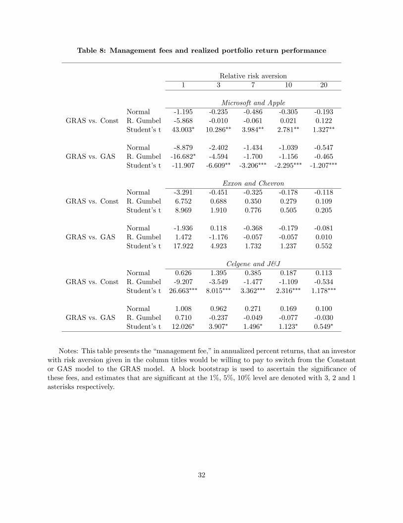
Table 8: Management fees and realized portfolio return performance
Relative risk aversion1 3 7 10 20
Microsoft and AppleNormal -1.195 -0.235 -0.486 -0.305 -0.193
GRAS vs. Const R. Gumbel -5.868 -0.010 -0.061 0.021 0.122Student�s t 43.003� 10.286�� 3.984�� 2.781�� 1.327��
Normal -8.879 -2.402 -1.434 -1.039 -0.547GRAS vs. GAS R. Gumbel -16.682� -4.594 -1.700 -1.156 -0.465
Student�s t -11.907 -6.609�� -3.206��� -2.295��� -1.207���
Exxon and ChevronNormal -3.291 -0.451 -0.325 -0.178 -0.118
GRAS vs. Const R. Gumbel 6.752 0.688 0.350 0.279 0.109Student�s t 8.969 1.910 0.776 0.505 0.205
Normal -1.936 0.118 -0.368 -0.179 -0.081GRAS vs. GAS R. Gumbel 1.472 -1.176 -0.057 -0.057 0.010
Student�s t 17.922 4.923 1.732 1.237 0.552
Celgene and J&JNormal 0.626 1.395 0.385 0.187 0.113
GRAS vs. Const R. Gumbel -9.207 -3.549 -1.477 -1.109 -0.534Student�s t 26.663��� 8.015��� 3.362��� 2.316��� 1.178���
Normal 1.008 0.962 0.271 0.169 0.100GRAS vs. GAS R. Gumbel 0.710 -0.237 -0.049 -0.077 -0.030
Student�s t 12.026� 3.907� 1.496� 1.123� 0.549�
Notes: This table presents the �management fee,�in annualized percent returns, that an investorwith risk aversion given in the column titles would be willing to pay to switch from the Constantor GAS model to the GRAS model. A block bootstrap is used to ascertain the signi�cance ofthese fees, and estimates that are signi�cant at the 1%, 5%, 10% level are denoted with 3, 2 and 1asterisks respectively.
32
15 10 5 0 5 10 1515
10
5
0
5
10
15
Microsoft
App
le
Dai ly returns
15 10 5 0 5 10 1515
10
5
0
5
10
15
Exxon
Che
vron
15 10 5 0 5 10 1515
10
5
0
5
10
15
Celgene
J&J
Figure 1: This �gure shows a scatter plot of daily returns on three pairs of stocks. We use dataover the period January 2000 to December 2010.
33

Jan00 Jan02 Jan04 Jan06 Jan08 Jan10
0.2
0.3
0.4
0.5
0.6
0.7Microsoft and Apple
Jan00 Jan02 Jan04 Jan06 Jan08 Jan10
0.4
0.6
0.8
Exxon and Chevron
Jan00 Jan02 Jan04 Jan06 Jan08 Jan10
0
0.2
0.4
0.6
Celgene and J&J
GRASGAS
Figure 2: This �gure shows the estimated correlation parameter of the Student�s t GRAS model(solid line) against the estimated correlation parameter of the Student�s t GAS model (dotted line)for three di¤erent pairs of stocks.
34

Jan06 Jan07 Jan08 Jan09 Jan10
0.5
0
0.5
1GRAS portfolio weights
MicrosoftApple
Jan06 Jan07 Jan08 Jan09 Jan100.4
0.2
0
0.2
0.4
0.6
0.8 ExxonChevron
Jan06 Jan07 Jan08 Jan09 Jan10
0.2
0
0.2
0.4
0.6CelgeneJ&J
Figure 3: This �gure shows the estimated optimal portfolio weights based on the Student�s t GRASmodel, for an investor with risk aversion of 7, for three pairs of assets.
35