Convex Transversals

Esther M. Arkin∗ Claudia Dieckmann† Christian Knauer‡

Joseph S. B. Mitchell∗ Valentin Polishchuk§ Lena Schlipf† Shang Yang¶

Abstract

We answer the question initially posed by Arik Tamir at the Fourth NYU Computa-tional Geometry Day (March, 1987): “Given a collection of compact sets, can one decide inpolynomial time whether there exists a convex body whose boundary intersects every set inthe collection?”

We prove that when the sets are segments in the plane, deciding existence of the convexstabber is NP-hard. The problem remains NP-hard if the sets are scaled copies of a convexpolygon. We also show that in 3D the stabbing problem is hard when the sets are balls.On the positive side, we give a polynomial-time algorithm to find a convex transversal of amaximum number of pairwise-disjoint segments (or convex polygons) in 2D if the verticesof the transversal are restricted to a given set of points.

We also consider stabbing with vertices of a regular polygon – a problem closely relatedto approximate symmetry detection: Given a set of disks in the plane, is it possible tofind a point per disk so that the points are vertices of a regular polygon? We show thatthe problem can be solved in polynomial time, and give an algorithm for an optimizationversion of the problem.

1 Introduction

Let S be a finite set of line segments in the plane. We say that S is stabbable if there exists aconvex polygon whose boundary C intersects every segment in S; the closed convex chain C isthen called a (convex) transversal or stabber of S.

Research on transversals is an old and rich area. Most of the work, however, has focusedon line transversals, i.e., on determining properties of families of lines that stab sets of var-ious types of geometric objects. Stabbing has attracted interest from various perspectives:purely combinatorial (complexity of the set of transversals, orders induced by stabbers), algo-rithmic (computing the stabbers), and applied (using transversals in curve reconstruction, linesimplification, graphics, motion planning) – see [12] and references therein. In some of theseapplications it is natural to consider convex transversals as generalizations of line transversals.For example, it may be of interest to establish whether the data collected in an experiment isconsistent with the assumption that the measured value is a convex function of the input. Inthis case, instead of fitting a linear function into the noisy measurements (a classical regressionproblem; see, e.g., [1] for an application in wireless sensor networks), one has to fit a convex

∗Department of Applied Mathematics and Statistics, Stony Brook University, USA.{estie,jsbm}@ams.stonybrook.edu†Institute of Computer Science, Freie Universitat Berlin, Germany. {dieck,schlipf}@mi.fu-berlin.de‡Institute of Computer Science, Universitat Bayreuth, Germany. christian.knauer@uni-bayreuth.de§Department of Computer Science, University of Helsinki, Finland. polishch@helsinki.fi¶Mathworks, USA. yangshang1985@gmail.com

1

function, i.e., to solve a non-parametric convex regression problem (see, e.g., [5, 9] for recentwork on convex regression).

The problem of computing a convex transversal for line segments was posed in 1987 [14]. Forthe case of stabbing vertical line segments, an optimal algorithm for the problem was presentedby Goodrich and Snoeyink in [8]. They stated the problem of finding a convex stabber for a setof arbitrary segments in the plane as open. To the best of our knowledge, there has been noprogress on the problem in the roughly 20 years since then.

Note that we address the decision problem – can a given set of objects be stabbed by theboundary of a convex polygon? A different line of work (see [6] for the recent results) considers anoptimization version – find a minimum-perimeter polygon whose boundary or interior intersectsa given set of segments.

Contributions

We prove that finding a convex transversal for a set of segments in the plane is NP-hard; theproblem remains NP-hard for a set of scaled copies of a given convex polygon. We also showthat in 3D, it is NP-hard to decide stabbability of a set of balls.

We then turn to positive results: Section 3 presents a dynamic program (DP) to decide ifa set of pairwise-disjoint segments is stabbable by a stabber whose vertices are a subset of agiven candidate set of points; if the segments are not stabbable, we can output a convex stabberthat intersects the maximum number of segments. The algorithm readily generalizes to the caseof disjoint convex polygons. (In an earlier version of the paper (see, e.g., [3]) we erroneouslyclaimed that there always exists a stabber with edges supported by bitangents between elementsof S. We also claimed that our algorithm extends directly to the case of convex pseudodisks;however, the details of that extension are not straightforward and will be the topic of a futurefollow-on paper.)

We also consider the approximate symmetry detection problem: Given a set of n disks inthe plane and an integer i, is it possible to find one point per disk such that the points form aset invariant under rotations by 2π/i? For general i, the problem is NP-hard [11]; in Section 4we give a polynomial-time algorithm for the case i = n. That is, we answer the question: is itpossible to find one point per disk such that the points are vertices of a regular polygon? Wealso consider an optimization variant of the problem: Given a set of points in the plane, findthe minimum δ∗ such that shifting each point by at most δ∗ brings the points into a symmetricposition.

Closed stabbers vs. Terrains The stabbing problem formulation is isotropic in the sensethat it does not single out any specific direction in the space. In function approximation andstatistics applications (unlike in surface reconstruction), it is often the case that the transversalrepresents the graph of a function. That is, the stabber is a terrain – a surface that intersectsevery vertical line in at most one point. A convex terrain is a part of the boundary of a convexpolygon (polytope in 3D).

Finding a convex terrain stabber is a special case of finding a convex stabber – to see this,just place one point far below the input (Figure 1). Our results, both positive and negative,are as strong as possible with respect to the distinction between convex terrain and convexstabbers: Our DP allows one to find even a convex stabber (and, hence, also to find a convexterrain stabber); our negative results show that it is hard already to find a convex terrain (and,hence, it is also hard to find a closed convex stabber).

2

p

S

Figure 1: S′ is S augmented with a point p. S can be stabbed by a convex terrain if and only if S′ has aconvex stabber. Thus, any algorithm that finds a stabber can also find a terrain. Conversely, if findinga terrain is hard, finding a stabber is also hard.

2 Hardness results

This section gives an answer to the question from [8,14] by showing that the problem is NP-hard.

2.1 Stabbing segments in the plane is NP-hard

Our reduction is from 3SAT. The reduction has the same spirit as the one used to show hardnessof finding the largest-area convex hull of a set of points that are restricted to lie on line segments[13]. As in [13], we “thread” variable and clause gadgets on a convex chain, and connect clausesto their literals with segments. The details of our construction (the gadgets themselves) aredifferent from [13].

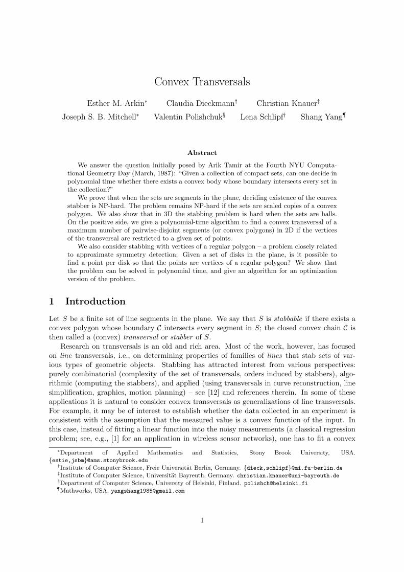
Our reduction is shown in Figures 2 and 3. We use n and m to denote the number of the3SAT variables and clauses, respectively.

Variable gadget For each variable we have a gadget that consists of three points (segmentsof zero length) and one segment. There are two ways to traverse the gadget (shown with dottedand dashed paths) that differ in the order in which the middle point and the segment are visited.The two ways correspond to setting the variable True or False. The important property of thegadget is that it will be possible to place a certain “connecting” segment in either of the twoways: so that it touches only the False subpath but not the True, and vice versa.

“Squashing” We make the variable gadget “thin” by moving all three points close to thesupporting line of the segment, and, in addition, by moving the non-middle points far apart.

Variable chain Variable gadgets are placed along a convex chain, called the variable chain.The chain is almost vertical, bending to the right only slightly. The variable gadgets are“clenched” onto the chain, and the distance between consecutive gadgets is large. Thus, theonly way to traverse the gadgets with a convex terrain is to visit them one by one, in the orderas they appear along the chain, assigning truth values to the variables in turn in each gadget.

Clause gadgets The clause gadgets are similarly arranged, one after one, on another almostvertical convex chain, slightly bending to the left; this clause chain is placed to the right of thevariable chain. Each clause gadget consists of 2 points and a segment; the only way to traverse

3

x1

x2

xn

C1

Cm

F

T

Figure 2: The variable gadget and the 2 ways to traverse it. The variable gadgets are threaded ontoa convex chain; similarly, the clause gadgets are threaded. The chains (dotted) are not parts of theconstruction and are shown only for reference. The clause gadget can be traversed in only one way.

F

T

F

T

F

Txi

xj

xk

C

Figure 3: A clause C = xi ∨ xj ∨ xk: three paths are shown that pick different subsets of the threeconnecting segments. The gadgets and their locations are not to scale: the gadgets are thinner, so thatthe points are very close to the supporting line of the segment – this makes the turn angles of the pathsclose to π; also, consecutive gadgets along each chain are separated so that a convex terrain can makeindependent choices in each of them.

the gadget is to visit the first point, then the segment and then the second point – the onlyflexibility is where to touch the segment.

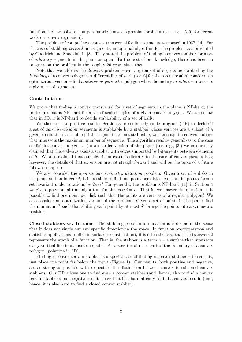
Connectors We now place 3m more segments, connecting a variable gadget to a clause gad-get whenever the variable appears in the clause (Figure 3). The placement of the segments’endpoints within variable gadgets is as follows: if the variable appears unnegated, the segmenttouches the True path through the gadget and does not intersect the False subpath; on thecontrary, if the variable appears negated, the segment touches only the False subpath. In everyclause gadget, segments’ endpoints look the same – see Figure 3; as can be easily checked,a convex terrain can intersect any two of the segments, but not all three. This finishes theconstruction.

The reduction If the 3SAT instance is feasible, the stabber can traverse the variable gadgetsaccording to the satisfying truth assignment. In each of the clauses, at least one of the connectingsegments (the one connecting to the satisfying variable) can be omitted; the other two are pickedup by one of the three paths.

Conversely, if there exists a stabber, it must omit (at least) one connecting segment perclause. Set the variable True or False depending on whether the omitted segment connectsfrom a True or False part of the variable gadget; this satisfies all the clauses. The True/Falsesetting is consistent because any segment omitted by the stabber in the clause gadget must

4

x1

x2

xn

C1

Cm

F

T

a1

a2

V

C

Figure 4: Left: Variable and clause gadgets (not to scale: each variable gadget is fit into the circulararc of length 1/(8n) and each clause gadget is fit into the circular arc of length 1/(8m); also consecutivegadgets are separated so that a convex terrain can make independent choices in each gadget). Right:V and C mark placements for variable and clause gadgets; the points a1, a2 ensure that the connectorsquares can either be intersected at a variable gadget or a clause gadget but nowhere else.

have been stabbed in the variable gadget, and there either only the True-subpath or only theFalse-subpath segments could have been stabbed, but not both.

We thus have our main negative result:

Theorem 2.1. Finding a convex (terrain) transversal for a set of segments in the plane isNP-hard.

In the remainder of this section we modify our proof to show hardness of stabbing scaledcopies of a convex polygon (Section 2.2) and hardness of stabbing balls in 3D (Section 2.3).

2.2 Stabbing squares and scaled copies of a convex polygon

To show hardness of stabbing squares we again reduce from 3SAT. The construction (Figure 4)is very similar to the one for segments.

Variable gadgets The variable gadget consists of three points (squares of zero area) anda square. The gadget is nearly the same as in the construction for segments, but instead ofa segment we use a square (the same holds for the clause gadgets). There are two ways totraverse a gadget; one corresponds to setting the variable True and the other to setting thevariable False.

“Fitting” We fit the variable gadget into a circular arc by putting the two non-middle pointson the arc. The middle point and the lower edge of the square (the edge that is closest to thethree points) lie inside the circular arc, see Figure 4. Each variable gadget is fit into an arc of1/(8n) of a unit circle.

Variable arc The variable gadgets are placed next to each other on an arc of one eighth ofa unit circle. We call this arc the variable arc. The only way to traverse the variable gadgetswith a convex terrain is to visit them one by one, in the order they appear on the arc, assigningtruth values in turn in each gadget.

5

F

F

T

xi

xj

xk

C

T

T

F

Figure 5: Clause C = xi ∨ xj ∨ xk. Three path are marked that pick up different subsets of the threeconnecting squares.

Clause gadgets The clause gadgets are placed in the same way as the variable gadgets, onan arc of one eighth of the unit circle and next to the variable arc. Each clause gadget consistsof two points and a square.

Connectors We place 3m more squares, connecting a variable gadget to a clause gadgetwhenever the variable appears in the clause (Figure 5). One edge of each square is placedexactly in the same way as the connector segment in the construction for line segments. Thismeans that one endpoint of the edge lies within the variable gadget as follows: if the variableappears unnegated, the edge touches the True subpath through the gadget and does not intersectthe False subpath; on the contrary, if the variable appears negated, the edge touches only theFalse subpath. In every clause gadget, the endpoints of these edges look the same.

To ensure that a convex terrain can intersect connecting squares only near the gadgets, weadd two points to the construction (Figure 4, right); a convex terrain that traverses these pointsand all gadgets cannot intersect the unit circle (on which the gadgets are placed) except at thegadgets. Thus, the connectors can be intersected only at endpoints of the edges that are placedin the same way as the connector segments in the construction for line segments. (Note that forthe latter property to hold, it was crucial to fit all variable and clause gadgets on the quarterof a unit circle – this way all connector squares lie inside the unit circle.)

The reduction Assume that the 3SAT formula is feasible. Then the stabber can traversethe variable gadgets according to the satisfying assignment. In each clause gadget one of thethree connecting squares has to be omitted by the stabber; let this be the one connecting tothe satisfying variable.

On the other hand, if there exists a stabber, it must omit at least one connecting square

6

per clause. Set the variables True or False depending on whether the omitted square connectsfrom a True or False path of the variable gadget; this satisfies all the clauses. This setting isconsistent since any square omitted by the stabber in the clause gadget has to be stabbed inthe variable gadget and there either only the True-subpath or the False-subpath squares couldhave been traversed, but not both.

Theorem 2.2. Finding a convex (terrain) transversal for a set of squares in the plane is NP-hard.

Generalization The above proof can be adapted to show that stabbing regular k-gons isNP-hard for any k > 2: just replace the squares with the k-gons, and (to ensure again that theconnectors lie inside the unit circle) place the variable and clause gadgets on an arc of 1/(2k)of a unit circle. That is, fit each variable gadget into an arc of 1/(4kn), and each clause gadgetinto an arc of 1/(4km).

Theorem 2.3. For arbitrary constant k > 2, finding a convex (terrain) transversal for a set ofregular k-gons in the plane is NP-hard.

It is not crucial that the polygons are regular, as only one edge of each polygon is importantfor the construction. Hence, the construction works in the same way if we consider a set ofscaled copied of a given polygon instead of regular polygons.

Theorem 2.4. Finding a convex (terrain) transversal for a set of scaled copies of a given convexpolygon in the plane is NP-hard.

An interesting open question is whether stabbing disks is NP-hard. Our reduction abovedoes not extend to this case – the reason is that we want the connectors to lie inside the unitdisk onto which the variable and clause gadgets are threaded (this is needed to ensure that theconnectors cannot be stabbed outside the unit circle – the only places to stab them are nearthe gadgets).

2.3 Stabbing balls in 3D is NP-hard

We again reduce from 3SAT, employing similar ideas as those for segments in 2D.

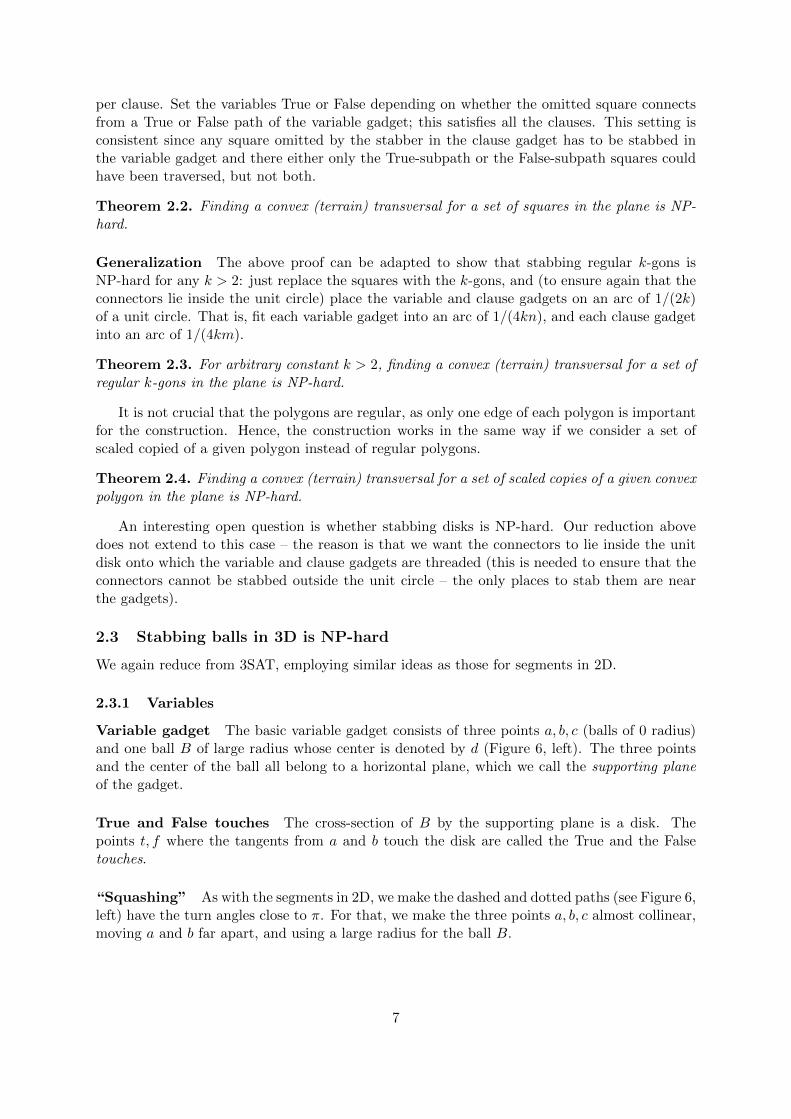
2.3.1 Variables

Variable gadget The basic variable gadget consists of three points a, b, c (balls of 0 radius)and one ball B of large radius whose center is denoted by d (Figure 6, left). The three pointsand the center of the ball all belong to a horizontal plane, which we call the supporting planeof the gadget.

True and False touches The cross-section of B by the supporting plane is a disk. Thepoints t, f where the tangents from a and b touch the disk are called the True and the Falsetouches.

“Squashing” As with the segments in 2D, we make the dashed and dotted paths (see Figure 6,left) have the turn angles close to π. For that, we make the three points a, b, c almost collinear,moving a and b far apart, and using a large radius for the ball B.

7

x1

x2

xn

F

Ta

b

c

d

x

y

z

x

y

z

x1x2

xn

xy z

strip

t

f

B

Figure 6: Left: The (cross-section by the supporting plane of the) variable gadget. The gadget is notto scale; actually, the turn angles of both the dashed and the dotted paths are close to π. Middle: Thevariable gadgets are threaded onto a convex chain; the chain (dotted) is not a part of the constructionand is shown only for reference. Right: The variable grid.

Variable chain Also as with segments in 2D, the variable gadgets are placed along an almost“flat” convex chain (Figure 6, middle). Again, the gadgets are “clenched” onto the chain sothat the three points of every gadget are very close to the chain. All gadgets and the chain arealigned, in that the supporting planes of all gadgets coincide, and the chain also lives in thiscommon horizontal plane. We thus also call the plane the supporting plane of the chain. Theballs are “sticking out” of the chain, i.e., the centers of the balls are placed outside the convexhull of the chain.

As with segments in 2D, consecutive gadgets along the chain are separated by large enoughdistance so that the cross-section of the stabber by the supporting plane must visit the gadgetsone by one, assigning truth values to the variables in turn in each gadget. We call this wholeconstruction—the gadgets threaded on the chain—the variable chain.

Variable grid We place m+ 2 copies of the variable chain, one copy directly above another(Figure 6, right). We number the copies from 0 to m + 1. The first and the last copies are“dummy”; we have them only to enforce consistency of the “choices” that the stabber mustmake in each of the chains (see below). The other copies correspond to the clauses.

We call the m+ 2 gadgets corresponding to variable xi in all m+ 2 chains the i-th variablestrip. This way, our construction so far is a “grid” of n strips × m+ 2 chains (see also Figure 8below).

Consistency In Section 2.3.4 we argue that any convex terrain must make the same “choices”at each of the m copies of the variable in a strip. That is, for all j = 1, . . . ,m, in the cross-section by the supporting plane of the jth chain, the stabber either uses the True touch or usesthe False touch.

2.3.2 Clauses

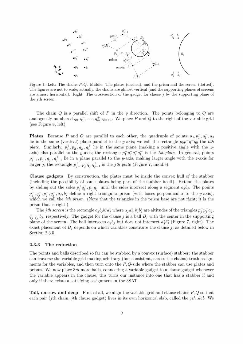
Clause chains Place 2(2m+2) points (0-radius balls) on two identical parallel almost verticalconvex chains P,Q, slightly bending to the left, lying in planes that are perpendicular to they-axis (Figure 7, left). More specifically, the first two points p0, p

−1 of P are the endpoints of

a segment parallel to the z-axis. The next two points, p+1 , p−2 are the endpoints of a segment

making a slightly larger than 0 angle with the z-axis. The next two points, p+2 , p−3 are endpoints

of a segment making even larger angle with the z-axis, and so on: the segments p+j p−j+1 make

larger and larger angles with the z-axis as j = 1, . . . ,m− 1 increases. The last two points of Pare p+m, pm+1. That is, P has 2 points per clause, plus the points p0, pm+1.

8

p0

p−1

p+1

p−2

p+2

p−3

yz q0

q−1

q+1

q−2

q+2

q−3

x

p+j

p−j

q+j

q−j

p+j−1

q+j−1

p−j+1

q−j+1

bj

aj

Bj

a∗j

b∗j

a∗j aj

b∗j bj

Bj

yz

x

plate

screen

prism

Figure 7: Left: The chains P,Q. Middle: The plates (dashed), and the prism and the screen (dotted).The figures are not to scale; actually, the chains are almost vertical (and the supporting planes of screensare almost horizontal). Right: The cross-section of the gadget for clause j by the supporting plane ofthe jth screen.

The chain Q is a parallel shift of P in the y direction. The points belonging to Q areanalogously numbered q0, q

−1 , . . . , q

+m, qm+1. We place P and Q to the right of the variable grid

(see Figure 8, left).

Plates Because P and Q are parallel to each other, the quadruple of points p0, p−1 , q

−1 , q0

lie in the same (vertical) plane parallel to the y-axis; we call the rectangle p0p−1 q−1 q0 the 0th

plate. Similarly, p+1 , p−2 , q

−2 , q

+1 lie in the same plane (making a positive angle with the z-

axis) also parallel to the y-axis; the rectangle p+1 p−2 q−2 q

+1 is the 1st plate. In general, points

p+j−1, p−j , q

−j , q

+j−1 lie in a plane parallel to the y-axis, making larger angle with the z-axis for

larger j; the rectangle p+j−1p−j q−j q

+j−1 is the jth plate (Figure 7, middle).

Clause gadgets By construction, the plates must be inside the convex hull of the stabber(including the possibility of some plates being part of the stabber itself). Extend the platesby sliding out the sides p+j q

+j , p

−j q−j until the sides intersect along a segment ajbj . The points

p+j , q+j , p

−j , q

−j , aj , bj define a right triangular prism (with bases perpendicular to the y-axis),

which we call the jth prism. (Note that the triangles in the prism base are not right; it is theprism that is right.)

The jth screen is the rectangle ajbjb∗ja∗j where aja

∗j , bjb

∗j are altitudes of the triangles p−j p

+j aj ,

q−j q+j bj , respectively. The gadget for the clause j is a ball Bj with the center in the supporting

plane of the screen. The ball intersects ajbj but does not intersect a∗jb∗j (Figure 7, right). The

exact placement of Bj depends on which variables constitute the clause j, as detailed below inSection 2.3.5.

2.3.3 The reduction

The points and balls described so far can be stabbed by a convex (surface) stabber: the stabbercan traverse the variable grid making arbitrary (but consistent, across the chains) truth assign-ments for the variables, and then turn onto the P,Q-side where the stabber can use plates andprisms. We now place 3m more balls, connecting a variable gadget to a clause gadget wheneverthe variable appears in the clause; this turns our instance into one that has a stabber if andonly if there exists a satisfying assignment in the 3SAT.

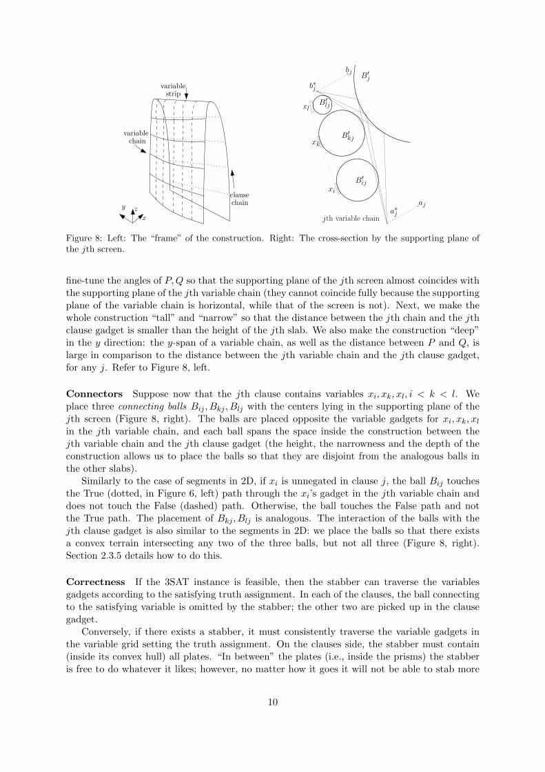
Tall, narrow and deep First of all, we align the variable grid and clause chains P,Q so thateach pair (jth chain, jth clause gadget) lives in its own horizontal slab, called the jth slab. We

9

x

y z

variablechain

clausechain

variablestrip

xi

xl

jth variable chain

xk

a∗j

b∗jB′j

B′lj

B′kj

B′ij

bj

aj

Figure 8: Left: The “frame” of the construction. Right: The cross-section by the supporting plane ofthe jth screen.

fine-tune the angles of P,Q so that the supporting plane of the jth screen almost coincides withthe supporting plane of the jth variable chain (they cannot coincide fully because the supportingplane of the variable chain is horizontal, while that of the screen is not). Next, we make thewhole construction “tall” and “narrow” so that the distance between the jth chain and the jthclause gadget is smaller than the height of the jth slab. We also make the construction “deep”in the y direction: the y-span of a variable chain, as well as the distance between P and Q, islarge in comparison to the distance between the jth variable chain and the jth clause gadget,for any j. Refer to Figure 8, left.

Connectors Suppose now that the jth clause contains variables xi, xk, xl, i < k < l. Weplace three connecting balls Bij , Bkj , Blj with the centers lying in the supporting plane of thejth screen (Figure 8, right). The balls are placed opposite the variable gadgets for xi, xk, xlin the jth variable chain, and each ball spans the space inside the construction between thejth variable chain and the jth clause gadget (the height, the narrowness and the depth of theconstruction allows us to place the balls so that they are disjoint from the analogous balls inthe other slabs).

Similarly to the case of segments in 2D, if xi is unnegated in clause j, the ball Bij touchesthe True (dotted, in Figure 6, left) path through the xi’s gadget in the jth variable chain anddoes not touch the False (dashed) path. Otherwise, the ball touches the False path and notthe True path. The placement of Bkj , Blj is analogous. The interaction of the balls with thejth clause gadget is also similar to the segments in 2D: we place the balls so that there existsa convex terrain intersecting any two of the three balls, but not all three (Figure 8, right).Section 2.3.5 details how to do this.

Correctness If the 3SAT instance is feasible, then the stabber can traverse the variablesgadgets according to the satisfying truth assignment. In each of the clauses, the ball connectingto the satisfying variable is omitted by the stabber; the other two are picked up in the clausegadget.

Conversely, if there exists a stabber, it must consistently traverse the variable gadgets inthe variable grid setting the truth assignment. On the clauses side, the stabber must contain(inside its convex hull) all plates. “In between” the plates (i.e., inside the prisms) the stabberis free to do whatever it likes; however, no matter how it goes it will not be able to stab more

10

than two connecting balls per clause. The unstabbed ball satisfies the clause; the consistencyof the satisfying assignment follows from the fact that a variable cannot be set both to Trueand to False by the same stabber.

Precision We were informal in saying that parts of the construction are “large” enough, “far”enough, etc. Still, the equations and inequalities involving the coordinates of the points in thegadgets have polynomial-size coefficients. E.g., a variable (resp. clause) chain can be part ofthe boundary of the regular O(n)-gon (resp. O(m)-gon). Thus, the construction can be done sothat it has the required properties and the coordinates specifying positions of the parts of thegadgets are polynomial in n and m.

Overall, we have:

Theorem 2.5. Finding a convex (terrain) transversal for a set of balls in 3D is NP-hard.

2.3.4 Consistency of choices in a variable strip

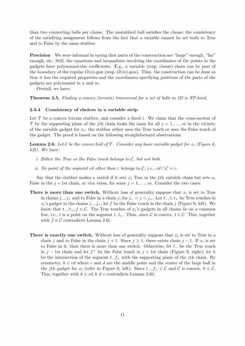
Let T be a convex terrain stabber, and consider a fixed i. We claim that the cross-section ofT by the supporting plane of the jth chain looks the same for all j = 1, . . . ,m in the vicinityof the variable gadget for xi: the stabber either uses the True touch or uses the False touch ofthe gadget. The proof is based on the following straightforward observations:

Lemma 2.6. Let C be the convex hull of T . Consider any basic variable gadget for xi (Figure 6,left). We have:

i. Either the True or the False touch belongs to C, but not both.

ii. No point of the segment cd other than c belongs to C; i.e., cd ∩ C = c.

Say that the stabber makes a switch if it sets xi True in the jth variable chain but sets xiFalse in the j + 1st chain, or vice versa, for some j = 1, . . . ,m. Consider the two cases:

There is more than one switch. Without loss of generality suppose that xi is set to Truein chains j−, j+ and to False in a chain j, for j− < j < j+. Let t−, t, t+ be True touches inxi’s gadget in the chains j−, j+; let f be the False touch in the chain j (Figure 9, left). Weknow that t−, t+, f ∈ C. The True touches of xi’s gadgets in all chains lie on a commonline, i.e., t is a point on the segment t−t+. Thus, since C is convex, t ∈ C. This, togetherwith f ∈ C contradicts Lemma 2.6i.

There is exactly one switch. Without loss of generality suppose that xi is set to True in achain j and to False in the chain j + 1. Since j ≥ 1, there exists chain j − 1. If xi is setto False in it, then there is more than one switch. Otherwise, let t− be the True touchin j − 1st chain and let f+ be the False touch in j + 1st chain (Figure 9, right); let hbe the intersection of the segment t−f+ with the supporting plane of the jth chain. Bysymmetry, h ∈ cd where c and d are the middle point and the center of the large ball inthe jth gadget for xi (refer to Figure 6, left). Since t−, f+ ∈ C and C is convex, h ∈ C.This, together with h ∈ cd, h 6= c contradicts Lemma 2.6ii.

11

F

a

b

c

t

f

T

j−

a

b

c

t+T

a

b

c

t− T

j

j+

z

F

a

b

c

t

f

Tj

j + 1

F f+

j − 1

t−T

h

Figure 9: Left: If f is in the stabber, then t is not; however if t−, t+ are in, then t must be in too. Right:If t−, f+ are in the stabber, then a point h 6= c of the segment cd is in the stabber.

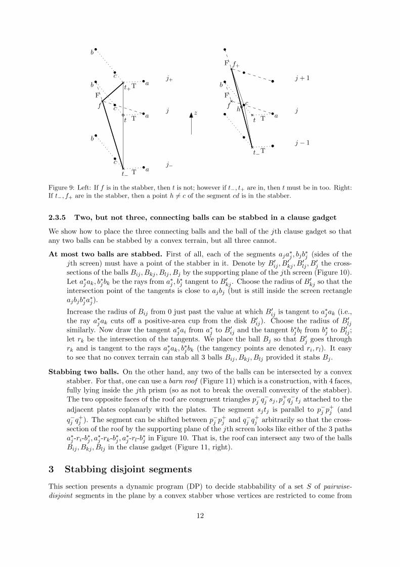
2.3.5 Two, but not three, connecting balls can be stabbed in a clause gadget

We show how to place the three connecting balls and the ball of the jth clause gadget so thatany two balls can be stabbed by a convex terrain, but all three cannot.

At most two balls are stabbed. First of all, each of the segments aja∗j , bjb

∗j (sides of the

jth screen) must have a point of the stabber in it. Denote by B′ij , B′kj , B

′lj , B

′j the cross-

sections of the balls Bij , Bkj , Blj , Bj by the supporting plane of the jth screen (Figure 10).Let a∗jak, b

∗jbk be the rays from a∗j , b

∗j tangent to B′kj . Choose the radius of B′kj so that the

intersection point of the tangents is close to ajbj (but is still inside the screen rectangleajbjb

∗ja∗j ).

Increase the radius of Bij from 0 just past the value at which B′ij is tangent to a∗jak (i.e.,the ray a∗jak cuts off a positive-area cup from the disk B′ij). Choose the radius of B′ljsimilarly. Now draw the tangent a∗jai from a∗j to B′ij and the tangent b∗jbl from b∗j to B′lj ;let rk be the intersection of the tangents. We place the ball Bj so that B′j goes throughrk and is tangent to the rays a∗jak, b

∗jbk (the tangency points are denoted ri, rl). It easy

to see that no convex terrain can stab all 3 balls Bij , Bkj , Blj provided it stabs Bj .

Stabbing two balls. On the other hand, any two of the balls can be intersected by a convexstabber. For that, one can use a barn roof (Figure 11) which is a construction, with 4 faces,fully lying inside the jth prism (so as not to break the overall convexity of the stabber).The two opposite faces of the roof are congruent triangles p−j q

−j sj , p

+j q−j tj attached to the

adjacent plates coplanarly with the plates. The segment sjtj is parallel to p−j p+j (and

q−j q+j ). The segment can be shifted between p−j p

+j and q−j q

+j arbitrarily so that the cross-

section of the roof by the supporting plane of the jth screen looks like either of the 3 pathsa∗j -ri-b

∗j , a∗j -rk-b

∗j , a∗j -rl-b

∗j in Figure 10. That is, the roof can intersect any two of the balls

Bij , Bkj , Blj in the clause gadget (Figure 11, right).

3 Stabbing disjoint segments

This section presents a dynamic program (DP) to decide stabbability of a set S of pairwise-disjoint segments in the plane by a convex stabber whose vertices are restricted to come from

12

xi

xl

jth variable chain

xk

a∗j

b∗j

bk

ak

bl

ai

rk

B′j

B′lj

B′kj

B′ij

rl

ri

bj

aj

Figure 10: The cross-section by the supporting plane of the jth screen.

a given discrete set C ⊂ R2 of candidate points. A subproblem in the DP is specified bya pair of potential stabber edges together with a constant-complexity “bridge” between theedges (the bridge is either a single segment or a segment—visibility-edge—segment chain). Thedisjointness of the segments allows us to determine which segments must be stabbed within thesubproblem. We show that a segment-free triangle can be found that separates a subprobleminto smaller subproblems, which allows the DP to recurse.

Arcs and nodes, chords and bridges A straight-line segment between two points from C(i.e., a potential stabber edge) is called an arc. Two arcs pq, rt are compatible if either they

13

p+j

p−j

q+j

q−j

p+j−1

q+j−1

p−j+1

q−j+1

bj

ajsj

tj

sj

tj

q−j

q+j−1

q−j−1

q+j−2

q−j−2

q+j

q−j+1

q+j+1

p−jp+j−1

p−j−1

p+j−2

p−j−2

p+j

p−j+1

p+j+1

Figure 11: Left: The roof. sjtj is below ajbj . sj (resp. tj) lies in the plane of the plate p+j−1p−j q−j q

+j−1

(resp. p−j+1p+j q

+j q−j+1). Right: View of the clause-side of the stabber from a point at +∞ on the x-axis;

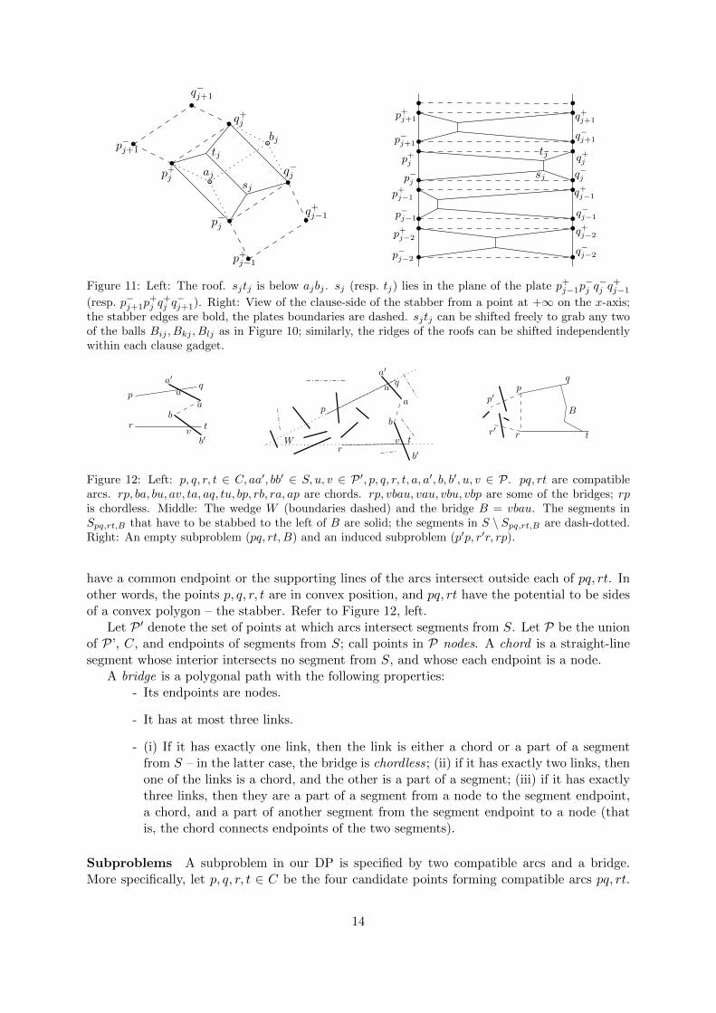
the stabber edges are bold, the plates boundaries are dashed. sjtj can be shifted freely to grab any twoof the balls Bij , Bkj , Blj as in Figure 10; similarly, the ridges of the roofs can be shifted independentlywithin each clause gadget.

u

ba

v

p

r

u

b

a

tW

a′

b′

a′

b′

r t

pq

B

r′

p′pq

r t

q

v

Figure 12: Left: p, q, r, t ∈ C, aa′, bb′ ∈ S, u, v ∈ P ′, p, q, r, t, a, a′, b, b′, u, v ∈ P. pq, rt are compatiblearcs. rp, ba, bu, av, ta, aq, tu, bp, rb, ra, ap are chords. rp, vbau, vau, vbu, vbp are some of the bridges; rpis chordless. Middle: The wedge W (boundaries dashed) and the bridge B = vbau. The segments inSpq,rt,B that have to be stabbed to the left of B are solid; the segments in S \ Spq,rt,B are dash-dotted.Right: An empty subproblem (pq, rt, B) and an induced subproblem (p′p, r′r, rp).

have a common endpoint or the supporting lines of the arcs intersect outside each of pq, rt. Inother words, the points p, q, r, t are in convex position, and pq, rt have the potential to be sidesof a convex polygon – the stabber. Refer to Figure 12, left.

Let P ′ denote the set of points at which arcs intersect segments from S. Let P be the unionof P’, C, and endpoints of segments from S; call points in P nodes. A chord is a straight-linesegment whose interior intersects no segment from S, and whose each endpoint is a node.

A bridge is a polygonal path with the following properties:- Its endpoints are nodes.

- It has at most three links.

- (i) If it has exactly one link, then the link is either a chord or a part of a segmentfrom S – in the latter case, the bridge is chordless; (ii) if it has exactly two links, thenone of the links is a chord, and the other is a part of a segment; (iii) if it has exactlythree links, then they are a part of a segment from a node to the segment endpoint,a chord, and a part of another segment from the segment endpoint to a node (thatis, the chord connects endpoints of the two segments).

Subproblems A subproblem in our DP is specified by two compatible arcs and a bridge.More specifically, let p, q, r, t ∈ C be the four candidate points forming compatible arcs pq, rt.

14

Without loss of generality let rt be below the line pq, and let q, p, r, t be the order in which thenodes appear counterclockwise on the convex hull of the arcs. We define the wedge W to bethe region that is below the line supporting pq and above the line supporting rt. In additionto the two arcs, the subproblem has in the input a bridge B that connects some point of pq tosome point of rt. Refer to Figure 12, middle.

Subproblem’s responsibility The crucial observation that allows us to run the DP is thefollowing: Assuming that the arcs pq, rt are part of the stabber, we know for each segments ∈ S whether it should be stabbed to the left or to the right of the bridge. Indeed, only thosesegments that have non-empty intersection with the wedge W can be stabbed. On the otherhand, no segment can have points on both sides of the bridge – for that it would have to crossthe bridge, and this is impossible: the chord is not crossed by definition, and no segment iscrossed by another segment due to the assumption of pairwise-disjointness of segments in S.

Let Spq,rt,B denote the segments that must be stabbed to the left of the bridge B; i.e., thesegments that intersect W in the part of the wedge that lies to the left of B.

The function Stab(·) Define a Boolean function Stab(pq, rt, B) to be True if the segmentsSpq,rt,B can be stabbed (assuming pq, rt is a part of the stabber), and to be False otherwise; foran incompatible pair of arcs pq, rt define Stab(pq, rt, ·) to be always False. The function showswhether the stabber can be “completed” having pq, rt as its part.

In the remainder of this section we show how to evaluate the function on a subproblem givenits values at other subproblems, i.e., how to solve the DP.

Empty subproblems The subproblem (pq, rt, B) is empty (Figure 12, right) if no segmentfrom S penetrates the region of W that is to the left of the bridge but to the right of rp (thisincludes the possibility that the bridge is the segment rp itself). An empty subproblem is closedif p = r. Closed subproblems are at the lowest level of our DP: clearly, Stab(σ) = True for aclosed subproblem σ.

Let (pq, rt, B) be an empty subproblem. We say that a subproblem (p′p, r′r, rp) is aninduced subproblem of (pq, rt, B) if pp′ is below (the supporting line of) pq, and rr′ is abovert. That is, the angles qpp′ and trr′ are convex, and thus both qpp′ and trr′ can potentiallybe parts of a convex chain – the stabber-to-be. Empty subproblems are easy to reduce toinduced subproblems: Stab(pq, rt, B) = True for an empty subproblem (pq, rt, B) if and only ifStab(p′p, r′r,B) is True for at least one subproblem induced by (pq, rt, B).

General subproblems Let C be the sought stabber that has pq, rt as two of the sides (Fig-ure 13). (Of course, we do not know C, but we will not use its existence in the algorithm, wewill only use C to argue that we can split the subproblem into smaller ones.) Let C’ be the(convex) region bounded by C, and let P be the part of C’ to the left of the bridge B (i.e., P iswhat is chopped off C’ by B). Consider the set P ′ = P \⋃s∈Spq,rt,B s. That is, P ′ is P “pierced”

by the segments Spq,rt,B that are stabbed in the subproblem (pq, rt, B).Because C is a stabber, every segment in Spq,rt,B intersects the boundary of P . This means

that P ′ is a (weakly) simple polygon (i.e., no segment makes a hole in P ′ by being fully containedin the interior of P ′). Each vertex of P ′ belongs to one of the following 6 (overlapping) sets:

P0: p, q, r, t

P1: vertices of the bridge;

P2: nodes that reside on the arcs pq, rt;

15

p

r

q

b

a

t

a′

b′

c

CP ′

B

Figure 13: The (unknown) part of the stabber C is dotted. P ′ is the simple polygon bounded by theunknown part of C, by pq, rt, by the bridge B = tbaq, and by the piercing segments. abc is a separating,i.e., segment-free triangle inside P ′.

p

r

q

b

a

t

a′

b′

c c′x

yz

CP ′

B

Figure 14: abc is a triangle in a triangulation of P ′; move c inside P ′. abz is the sought triangle.

P3: nodes that belong to C except those in P2;

P4: endpoints of segments from Spq,rt,B that are stabbed by pq or rt;

P5: endpoints of segments from Spq,rt,B that are stabbed by C \ pq, rt.

Note that only P3 is not known to us (because we do not know C); all the other sets are knownas soon as the subproblem (pq, rt, B) is specified.

We define the important link ba of the bridge B as follows: if B is chordless, then ba = B;otherwise ba is the chord of B. We assume that a is closer to pq, and b is closer to rt along B.Our algorithm will search for a separating, i.e., segment-free triangle abc within P ′ where c is avertex of P ′ and c /∈ P3 ∪P0. We first argue that such a triangle exists, and next describe whatto do depending on the set, among P1, P2, P4, P5, to which c belongs.

Lemma 3.1. There exists a vertex c of P ′ such that c /∈ P3 ∪P0 and no segment intersects theinterior of abc.

Proof. The link ba is a side of P ′; thus, any triangulation of P ′ has a triangle abc, with c beinga vertex of P ′. If there exists a triangulation such that c /∈ P3 ∪ P0, we are done. Otherwise,let xy be the segment that contains c; i.e., c = xy ∩ C (Figure 14). Move c along xy inside P ′.Either c reaches the endpoint of the segment (in which case we are done because c ∈ P5) or oneof the sides of abc, say, bc hits an endpoint z of a segment from Spq,rt,B; let c′ be the positionof c on xy when this happens. The convex quadrilateral cc′ba has no segments in the interior,and abz is the sought triangle. The case c ∈ P0 is treated similarly.

We emphasize that even though we used C in arguing the existence of the vertex as in theabove lemma, we can find such a vertex without knowing C (e.g., just by trying all vertices inP1, P2, P4, P5).

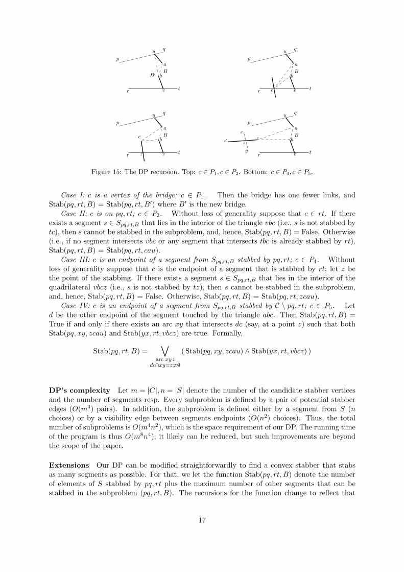
Let B = vbau be the bridge. We now show how our DP recurses into subproblems definedby the sides of the triangle abc (Figure 15):

16

p

r

q

b

a

t

BB′

v

u

p

r

q

b

a

t

B

c v

u

p

r

q

b

a

t

Bc

z v

u

p

r

q

b

a

t

zdc

Bx

yv

u

Figure 15: The DP recursion. Top: c ∈ P1, c ∈ P2. Bottom: c ∈ P4, c ∈ P5.

Case I: c is a vertex of the bridge; c ∈ P1. Then the bridge has one fewer links, andStab(pq, rt, B) = Stab(pq, rt, B′) where B′ is the new bridge.

Case II: c is on pq, rt; c ∈ P2. Without loss of generality suppose that c ∈ rt. If thereexists a segment s ∈ Spq,rt,B that lies in the interior of the triangle vbc (i.e., s is not stabbed bytc), then s cannot be stabbed in the subproblem, and, hence, Stab(pq, rt, B) = False. Otherwise(i.e., if no segment intersects vbc or any segment that intersects tbc is already stabbed by rt),Stab(pq, rt, B) = Stab(pq, rt, cau).

Case III: c is an endpoint of a segment from Spq,rt,B stabbed by pq, rt; c ∈ P4. Withoutloss of generality suppose that c is the endpoint of a segment that is stabbed by rt; let z bethe point of the stabbing. If there exists a segment s ∈ Spq,rt,B that lies in the interior of thequadrilateral vbcz (i.e., s is not stabbed by tz), then s cannot be stabbed in the subproblem,and, hence, Stab(pq, rt, B) = False. Otherwise, Stab(pq, rt, B) = Stab(pq, rt, zcau).

Case IV: c is an endpoint of a segment from Spq,rt,B stabbed by C \ pq, rt; c ∈ P5. Letd be the other endpoint of the segment touched by the triangle abc. Then Stab(pq, rt, B) =True if and only if there exists an arc xy that intersects dc (say, at a point z) such that bothStab(pq, xy, zcau) and Stab(yx, rt, vbcz) are true. Formally,

Stab(pq, rt, B) =∨

arc xy :dc∩xy=z 6=∅

( Stab(pq, xy, zcau) ∧ Stab(yx, rt, vbcz) )

DP’s complexity Let m = |C|, n = |S| denote the number of the candidate stabber verticesand the number of segments resp. Every subproblem is defined by a pair of potential stabberedges (O(m4) pairs). In addition, the subproblem is defined either by a segment from S (nchoices) or by a visibility edge between segments endpoints (O(n2) choices). Thus, the totalnumber of subproblems is O(m4n2), which is the space requirement of our DP. The running timeof the program is thus O(m8n4); it likely can be reduced, but such improvements are beyondthe scope of the paper.

Extensions Our DP can be modified straightforwardly to find a convex stabber that stabsas many segments as possible. For that, we let the function Stab(pq, rt, B) denote the numberof elements of S stabbed by pq, rt plus the maximum number of other segments that can bestabbed in the subproblem (pq, rt, B). The recursions for the function change to reflect that

17

Stab(pr, qt, B) is the sum of the values of the function on the subproblems. Further, our DPextends immediately to solve the convex stabbing problem for disjoint convex polygons.

4 Stabbing with vertices of a regular polygon

In this section we present an algorithm to decide whether a given set of disks can be stabbed bya regular polygon. Specifically, the approximate symmetry detection problem is: Given a setof n disks in the plane and an integer i, is it possible to find one point per disk such that thepoints form a set invariant under rotations by 2π/i? While the problem is NP-hard for generali [11], we solve the case i = n, i.e., we determine whether it is possible to find one point perdisk so that the points are vertices of a regular n-gon.

4.1 The decision problem

Let D = {d1, . . . , dn} be the given disks. For points p, c ∈ R2 and integer k ≤ n let ρkc (p) denotethe image of p after rotation around c by the angle k2π/n. For a pair of disks di, dj ∈ D, letAkij = {(p, c)|c ∈ R2, p ∈ di, ρkc (p) ∈ dj} ⊂ R4 be the set of all pairs (p, c) of points p ∈ di, c ∈ R2

such that p moves to dj after rotating by k2π/n around c; we call Akij the apex region.Fix a disk d1. A regular n-gon with a vertex per disk of D exists if and only if there exist

p ∈ d1 and c ∈ R2 (the center of the n-gon) such that ρjc(p) ∈ dj+1 for j = 1, . . . , n − 1, or

in other words, if and only if the intersection of n − 1 apex regions Aj1j+1 is non-empty (herethe vertices of the regular n-gon stab the disks in the order d1, d2, . . .; of course this order isnot known in advance). This prompts us to go through “all possible” intersections between theapex regions, checking for each of the intersections whether an n-gon exists.

Specifically, consider the (n − 1)2 apex regions Ak1,j , j = 2, . . . , n, k = 1, . . . , n − 1. Call a

point (p, c) ∈ R4 feasible if it belongs to some n− 1 of the regions, with each region being froma different disk with a different angle. Our problem has a feasible solution if and only if thereexists a feasible point in R4.

There are O(n2) apex regions, and each is defined by 2 polynomials of constant degree; thus,the arrangement of the regions has polynomial complexity. The feasibility of a point in R4 doesnot change as the point moves inside the cell of the arrangement; hence, in order to determineexistence of a feasible point, it is enough to check the feasibility of an arbitrary representativepoint r = (p, c) inside every cell. By [4], a representative for each cell can be obtained in O(n2)time.

To check if r = (p, c) is feasible, build the bipartite graph Gr; the n− 1 nodes on one partcorrespond to the disks D \ d1, the n − 1 nodes on the other part correspond to the angles{π/n, 4π/n, 6π/n, . . . , (n − 1)2π/n}. There is an edge between a disk node dj and an anglenode k2π/n if p rotated around c by the angle k2π/n lands in dj (i.e., ρkc (p) ∈ dj). There is aperfect matching in Gr if and only if c is the center of a regular n-gon with vertices in the disksfrom D.

Running time Each apex region consists of 2 algebraic surfaces in R4; thus, the arrangementdefined by all surfaces consists of O(n8) cells. It takes O(n10) time to compute a representativefor each cell [4]. For each representative of a cell we compute the corresponding bipartite graphand check if the graph has a perfect matching. A maximum matching in a bipartite graphwith n nodes and m edges can be computed in O(m

√n) time [10]. Since the graphs Gr and

Gr′ differ in only one edge whenever r and r′ lie in neighboring cells, we can use a dynamicmatching algorithm. We traverse the cells in depth first search order. Each update in the

18

dynamic matching algorithm can be done in O(m) time [2]. Thus, the total running time forour algorithm is O(n10).

The above algorithm can be used for objects other than disks, only the running time willchange depending on the complexity of the apex regions.

4.2 Optimization problem: Symmetry with imprecision

We now consider the following problem: Given a set P = {p1, . . . , pn} of n points, find theminimum δ∗ such that shifting each point by at most δ∗ brings the points in symmetric position(which means they are vertices of a regular n-gon). We give an exact algorithm, a quickconstant-factor approximation, and a PTAS for the problem.

4.2.1 Exact solution

It is immediate that in the optimal solution, some J points of P are shifted by exactly δ∗; weargue that J ≤ 5. Renumber the points in P so that the points shifted by δ∗ are p1, . . . , pJ , andlet q1, . . . , qJ be the shifted points. Suppose we know that qj is the kj-th vertex of the optimaln-gon, where k1, . . . , kJ are some distinct integers between 1 and n. We can then write oneequation for each j = 1, . . . , J :

|Rkj 2πn (pj − c)− (q1 − c)| = δ∗

where c is the center of symmetry of the n-gon and Rkj2π/n is the rotation matrix with rotationangle kj2π/n. Overall, we have J equations in 5 variables (two for each of c and q1, and onefor δ∗) . The system has a solution with an isolated δ∗ when J = 5.

The above observations lead to a (high) polynomial-time algorithm for the problem: Guess5 points of P and 5 numbers k1, . . . , k5. For each guess, solve the above described system of5 equations in 5 unknowns to get (a constant number of) candidate values for δ∗; for eachcandidate run the symmetry detection algorithm from Section 4.1 with radius-δ∗ disks centeredon points of P in the input.

4.2.2 O(1)-approximations

We start with two auxiliary lemmas:

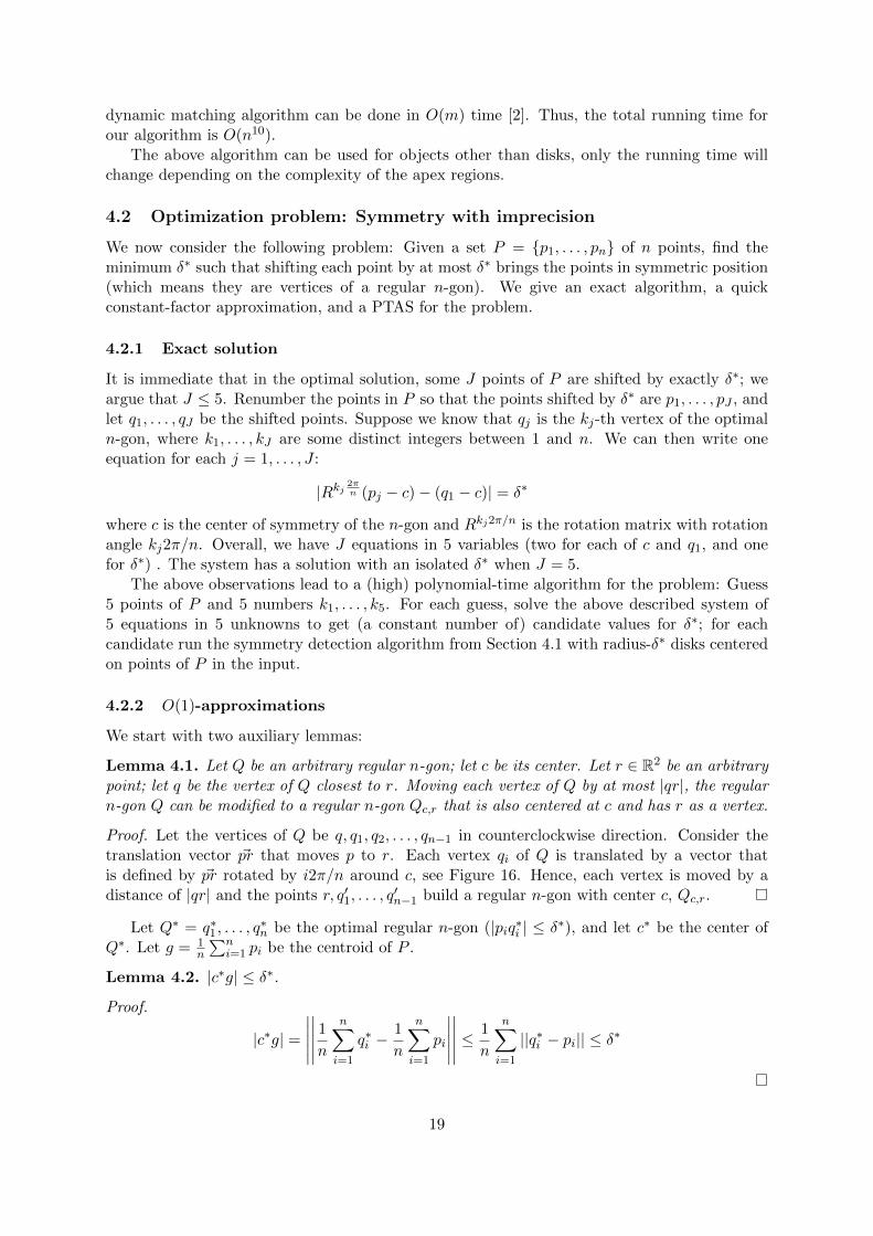
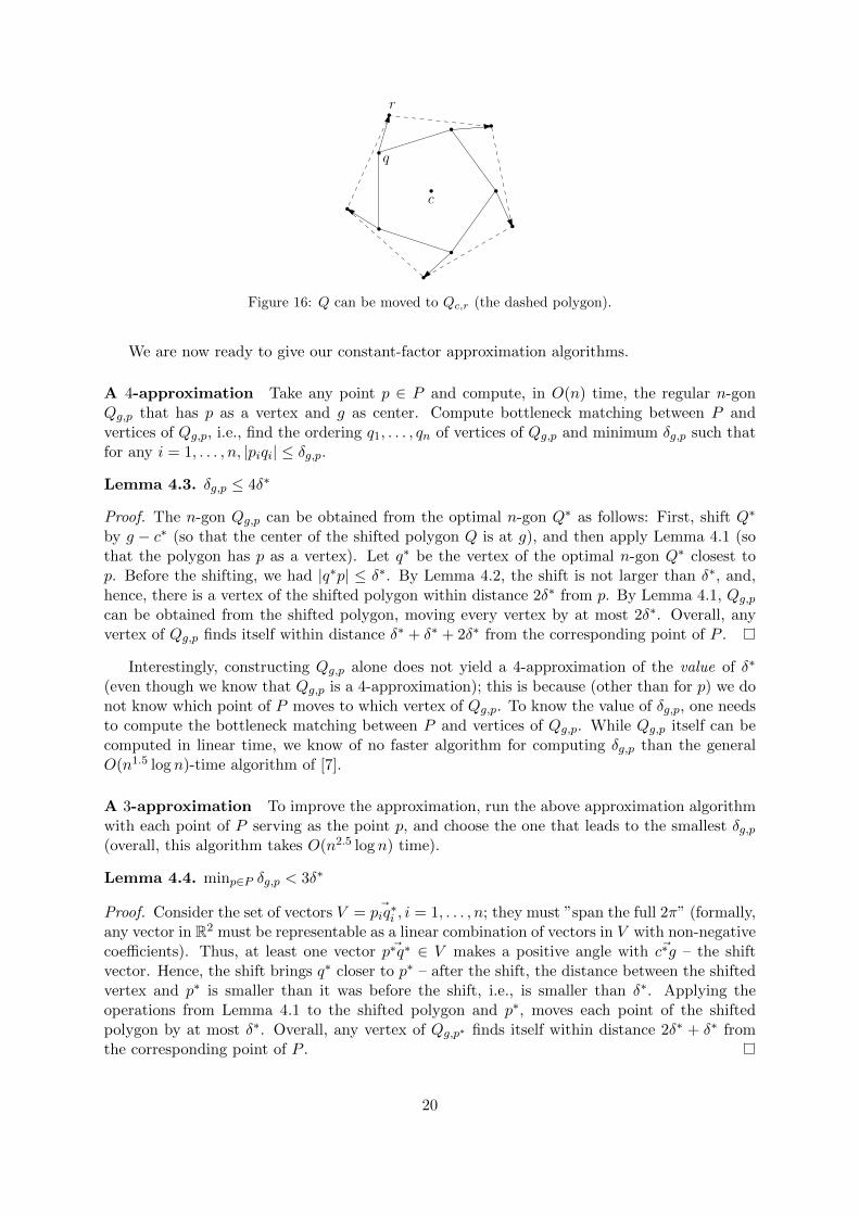
Lemma 4.1. Let Q be an arbitrary regular n-gon; let c be its center. Let r ∈ R2 be an arbitrarypoint; let q be the vertex of Q closest to r. Moving each vertex of Q by at most |qr|, the regularn-gon Q can be modified to a regular n-gon Qc,r that is also centered at c and has r as a vertex.

Proof. Let the vertices of Q be q, q1, q2, . . . , qn−1 in counterclockwise direction. Consider thetranslation vector ~pr that moves p to r. Each vertex qi of Q is translated by a vector thatis defined by ~pr rotated by i2π/n around c, see Figure 16. Hence, each vertex is moved by adistance of |qr| and the points r, q′1, . . . , q

′n−1 build a regular n-gon with center c, Qc,r.

Let Q∗ = q∗1, . . . , q∗n be the optimal regular n-gon (|piq∗i | ≤ δ∗), and let c∗ be the center of

Q∗. Let g = 1n

∑ni=1 pi be the centroid of P .

Lemma 4.2. |c∗g| ≤ δ∗.Proof.

|c∗g| =∣∣∣∣∣∣∣∣∣∣ 1n

n∑i=1

q∗i −1

n

n∑i=1

pi

∣∣∣∣∣∣∣∣∣∣ ≤ 1

n

n∑i=1

||q∗i − pi|| ≤ δ∗

19

q

r

c

Figure 16: Q can be moved to Qc,r (the dashed polygon).

We are now ready to give our constant-factor approximation algorithms.

A 4-approximation Take any point p ∈ P and compute, in O(n) time, the regular n-gonQg,p that has p as a vertex and g as center. Compute bottleneck matching between P andvertices of Qg,p, i.e., find the ordering q1, . . . , qn of vertices of Qg,p and minimum δg,p such thatfor any i = 1, . . . , n, |piqi| ≤ δg,p.

Lemma 4.3. δg,p ≤ 4δ∗

Proof. The n-gon Qg,p can be obtained from the optimal n-gon Q∗ as follows: First, shift Q∗

by g − c∗ (so that the center of the shifted polygon Q is at g), and then apply Lemma 4.1 (sothat the polygon has p as a vertex). Let q∗ be the vertex of the optimal n-gon Q∗ closest top. Before the shifting, we had |q∗p| ≤ δ∗. By Lemma 4.2, the shift is not larger than δ∗, and,hence, there is a vertex of the shifted polygon within distance 2δ∗ from p. By Lemma 4.1, Qg,pcan be obtained from the shifted polygon, moving every vertex by at most 2δ∗. Overall, anyvertex of Qg,p finds itself within distance δ∗ + δ∗ + 2δ∗ from the corresponding point of P .

Interestingly, constructing Qg,p alone does not yield a 4-approximation of the value of δ∗

(even though we know that Qg,p is a 4-approximation); this is because (other than for p) we donot know which point of P moves to which vertex of Qg,p. To know the value of δg,p, one needsto compute the bottleneck matching between P and vertices of Qg,p. While Qg,p itself can becomputed in linear time, we know of no faster algorithm for computing δg,p than the generalO(n1.5 log n)-time algorithm of [7].

A 3-approximation To improve the approximation, run the above approximation algorithmwith each point of P serving as the point p, and choose the one that leads to the smallest δg,p(overall, this algorithm takes O(n2.5 log n) time).

Lemma 4.4. minp∈P δg,p < 3δ∗

Proof. Consider the set of vectors V = ~piq∗i , i = 1, . . . , n; they must ”span the full 2π” (formally,any vector in R2 must be representable as a linear combination of vectors in V with non-negativecoefficients). Thus, at least one vector ~p∗q∗ ∈ V makes a positive angle with ~c∗g – the shiftvector. Hence, the shift brings q∗ closer to p∗ – after the shift, the distance between the shiftedvertex and p∗ is smaller than it was before the shift, i.e., is smaller than δ∗. Applying theoperations from Lemma 4.1 to the shifted polygon and p∗, moves each point of the shiftedpolygon by at most δ∗. Overall, any vertex of Qg,p∗ finds itself within distance 2δ∗ + δ∗ fromthe corresponding point of P .

20

A PTAS Compute a 4-approximation δ of δ∗, and lay out 1ε × 1

ε grids Gg and Gp in theδ-neighborhood of g and the δ-neighborhood of some point p ∈ P , respectively. Then, for eachpair (g′, p′) of grid points from Gg ×Gp, compute the regular polygon Qg′,p′ centered at g′ andhaving a vertex at p′, and find the value δg′,p′ of the bottleneck matching between P and thevertices of Qg′,p′ ; this can be done in overall O( 1

ε4n1.5 log n) time.

Lemma 4.5. ming′,p′ δg′,p′ ≤ (1 +O(ε))δ∗

Proof. Some vertex q∗ of Q∗ is within distance δ from p; thus, q∗ is within distance O(εδ∗) fromsome gridpoint p∗ ∈ Gp. Shift the optimal polygon Q∗ so that its center c∗ moves onto theclosest point g∗ ∈ Gg. The shift moves each vertex of Q∗ by O(εδ∗); in particular, the shiftedq∗ remains O(εδ∗)-close to p∗. Applying Lemma 4.1, we obtain that each vertex of Qg∗,p∗ findsitself within distance δ∗ +O(εδ∗) +O(εδ∗) from the corresponding vertex of P .

5 Conclusion

We resolved a long-standing open question: Can one determine in polynomial time whether aset of objects has a convex transversal? We gave negative answers for segments and scaled copiesof a convex polygon in 2D and for balls in 3D. Our construction showing hardness of stabbingnon-disjoint segments in 2D can be lifted to 3D while removing the intersections between thesegments; hence, stabbing disjoint objects in 3D is also hard.

Note that the segments/balls used in our hardness proofs are of drastically different sizes(in particular, we used zero-length segments and zero-volume balls which might be consideredas somewhat artificial). Our construction for the segments can be easily extended to the casewhere all segments have length between 1 and 1 + ε for any ε > 0; we believe that similarextension is possible for the balls. However, for unit segments/balls our constructions fails. Weleave these as open problems.

On the positive side, we gave a polynomial-time algorithm to determine a convex stabber,if it exists, for a set of disjoint line segments or disjoint convex polygons under the restrictionthat the stabber vertices come from a given set C of candidate points. The most intriguingopen question is whether the restriction can be removed. Another open question is whetherthere are non-trivial lower bounds on the complexity of algorithms for finding transversals.

In general, convex transversals open a whole new research direction. Apart from the algo-rithmic study, it could be of interest to investigate combinatorial properties of convex stabbers,e.g., the number of geometric permutations induced by convex stabbers for different classes ofobjects.

Acknowledgments

We thank Joe Blitzstein (Harvard University) for pointers to work in convex regression, andthe anonymous reviewer for helpful comments. E. Arkin and J. Mitchell are partially supportedby the National Science Foundation (CCF-0729019, CCF-1018388). Work by L. Schlipf wassupported by the Deutsche Forschungsgemeinschaft within the research training group “Methodsfor Discrete Structures”(GRK 1408). V. Polishchuk is supported by the Academy of Finlandgrant 138520.

References

[1] P. K. Agarwal, A. Efrat, C. Gniady, J. S. B. Mitchell, V. Polishchuk, and G. Sabhnani. Dis-tributed localization and clustering using data correlation and the Occam’s razor principle.

21

In 7th International Conference on Distributed Computing in Sensor Systems (DCOSS),pages 1–8. IEEE, 2011.

[2] D. Alberts and M. R. Henzinger. Average case analysis of dynamic graph algorithms. InSODA ’95, pages 312–321, 1995.

[3] E. M. Arkin, J. S. B. Mitchell, V. Polishchuk, and S. Yang. Convex transversals. In FallWorkshop on Computational Geometry, 2010.

[4] S. Basu, R. Pollack, and M.-F. Roy. On computing a set of points meeting every cell definedby a family of polynomials on a variety. J. Complex., 13(1):28–37, 1997.

[5] M. Birke and H. Dette. Estimating a convex function in nonparametric regression. Scan-dinavian Journal of Statistics, 34(2):384–404, 2007.

[6] A. Dumitrescu and M. Jiang. Minimum-perimeter intersecting polygons. Algorithmica,63(3):602–615, 2012.

[7] A. Efrat, A. Itai, and M. J. Katz. Geometry helps in bottleneck matching and relatedproblems. Algorithmica, 31(1):1–28, 2001.

[8] M. T. Goodrich and J. Snoeyink. Stabbing parallel segments with a convex polygon.Comput. Vision Graph. Image Process., 49(2):152–170, 1990.

[9] P. Groeneboom, G. Jongbloed, and J. A. Wellner. Estimation of a convex function: char-acterizations and asymptotic theory. The Annals of Statistics, 29(6):1653–1698, 2001.

[10] J. Hopcroft and R. M. Karp. An n(5/2) algorithm for maximum matchings in bipartitegraphs. SIAM J. Comput., 2(4):225–231, 1973.

[11] S. Iwanowski. Testing approximate symmetry in the plane is NP-hard. Theor. Comput.Sci., 80(2):227–262, 1991.

[12] H. Kaplan, N. Rubin, and M. Sharir. Line transversals of convex polyhedra in R3. SIAMJ. Comput., 39(7):3283–3310, 2010.

[13] M. Loffler and M. J. van Kreveld. Largest and smallest convex hulls for imprecise points.Algorithmica, 56(2):235–269, 2010.

[14] A. Tamir. Problem 4-2 (New York University, Dept. of Statistics and Operations Research),Problems Presented at the Fourth NYU Computational Geometry Day (3/13/87).

22