primal dual algorithms for convex optimization in …eesser/papers/maipcv2011.pdfprimal dual...

Primal Dual Algorithms for ConvexOptimization in Imaging Science

Ernie Esser

UC Irvine

MAIPCV2011 Winter School, Tohoku University

11-25-2011

1

Variational Models (1)

A powerful modeling tool in image processing and computer vision is toconstruct a functional such that its minimizer(s) are good solutions to theproblem of interest.A general form:

minu∈Rm

J(u) such that Au = b

Common difficulties:• Image and video problems are large with many variables• Models often involve nonsmooth objective functions

2

Variational Models (2)

minu∈Rm


Common advantages:

• Separable structure:

J(u) =

n∑

i=1

Ji(ui) u =

u1

...

uN

N ≥ n

with simple functionsJi• Convex: J((1− s)u+ sv) ≤ (1− s)J(u) + sJ(v) for all u, v

s ∈ (0, 1)

Goal: Study and develop practical algorithms for minimizing large,nonsmooth convex functions with separable structure.

3

Convexity

In fact the great watershed in optimization isn’t between linearity andnonlinearity, but convexity and nonconvexity.

- R. T. Rockafellar

Let us first look at some illustrative examples of large, nonlinear, nonsmoothconvex models in image processing which can be effectively solved using theprimal-dual algorithms which will be discussed later:

4

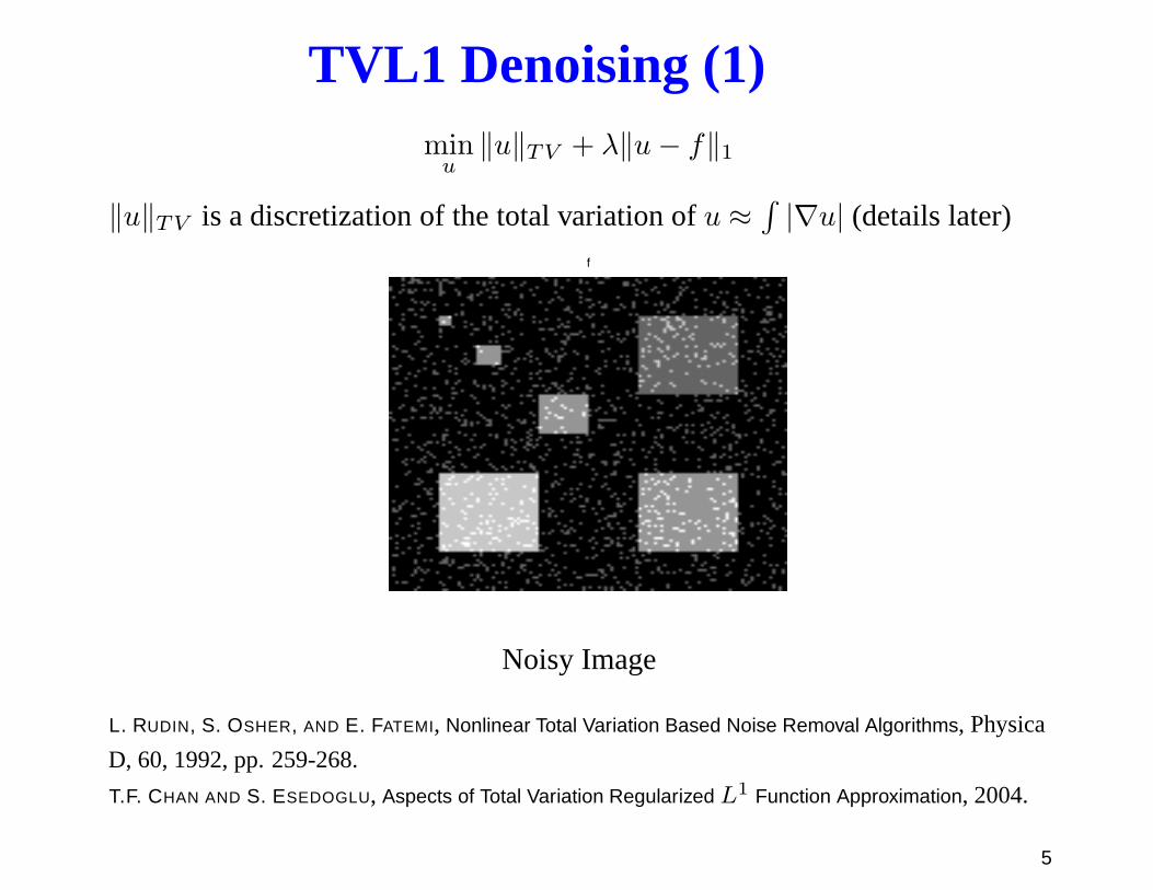
TVL1 Denoising (1)minu

‖u‖TV + λ‖u− f‖1

‖u‖TV is a discretization of the total variation ofu ≈∫

|∇u| (details later)f

Noisy Image

L. RUDIN, S. OSHER, AND E. FATEMI, Nonlinear Total Variation Based Noise Removal Algorithms, Physica

D, 60, 1992, pp. 259-268.

T.F. CHAN AND S. ESEDOGLU, Aspects of Total Variation Regularized L1 Function Approximation, 2004.

5

TVL1 Denoising (2)

u

Recovered Image

6

TVL1 Denoising (3)

f−u

Sparse Error

7

Constrained TVL2 Deblurring

minu

‖u‖TV such that ‖k ∗ u− f‖2 ≤ ǫ

Original, blurry/noisy and image recovered from 300 iterations

E. ESSER, X. ZHANG, AND T. F. CHAN, A General Framework for a Class of First Order Primal-Dual

Algorithms for Convex Optimization in Imaging Science, SIAM J. Imaging Sci. Volume 3, Issue 4,

2010.

8

Sparse/Low Rank Decomposition (1)minu,e

‖u‖∗ + λ‖e‖1 such that f = u+ e

Here,‖u‖∗ denotes the nuclear norm, which is the sum of the singular valuesof u.

original movie

Original Video

E. CANDES, X. LI, Y. MA AND J. WRIGHT, Robust Principal Component Analysis, 2009.

9

Sparse/Low Rank Decomposition (2)

low rank part

Recovered Backgroundu 10

Sparse/Low Rank Decomposition (3)

sparse error

Sparse Errore 11

Multiphase Segmentation (1)Many problems deal with the normalization constraintc ∈ C, where

C = {c = (c1, ..., cW ) : cw ∈ RM ,

W∑

w=1

cw = 1, cw ≥ 0}

Example: Convex relaxation of multiphase segmentation

Goal: Segment a given image,h ∈ RM , intoW regions where the intensities

in thewth region are close to given intensitieszw ∈ R and the lengths of theboundaries between regions are not too long.

minc∈C

W∑

w=1

(

‖cw‖TV +λ

2〈cw, (h− zw)

2〉)

This is a convex approximation of the related nonconvex functional whichadditionally requires the labels,c, to only take on the values zero and one.

E. BAE, J. YUAN, AND X. TAI, Global Minimization for Continuous Multiphase Partitioning Problems Using a

Dual Approach, UCLA CAM Report [09-75], 2009.

C. ZACH, D. GALLUP, J.-M. FRAHM, AND M. NIETHAMMER, Fast global labeling for real-time stereo using

multiple plane sweeps, VMV, 2008. 12

Multiphase Segmentation (2)

λ = .0025 z =[

75 105 142 178 180]

Thresholdc when each‖ck+1w − ckw‖∞ < .01 (150 iterations)

original image segmented image

region 1 region 2 region 3 region 4 region 5

Segmentation of Brain Image Into5 RegionsModifications: We can also addµw parameters to regularize differently thelengths of the boundaries of each region and alternately update the averageszwhen they are not known beforehand.

13

Reductions to Standard Form

All the previous illustrative examples can be rewritten in the form

minu

∑

i

Ji(ui) such that Au = b u =

u1

...

uN

Sometimes this requires introducing additional variablesand constraints.

14

Constrained TVL2 Deblurring Example

minu

‖u‖TV such that ‖k ∗ u− f‖2 ≤ ǫ

LetD be a discrete gradient and‖ · ‖E anl1-like norm such that‖Du‖Ecorrseponds to our discretization of‖u‖TV (details later).

Introducew = Du andz = k ∗ u− f . An equivalent problem is:

minu,w,z

‖w‖E + gB(z) s.t. w −Du = 0 and z − k ∗ u = −f

gB(z) =

{

0 if ‖z‖2 ≤ ǫ

∞ otherwiseis a convex indicator function.

15

Convex Models for Nonconvex Problems

Convex optimization is still important for many nonconvex problems:

• Convex relaxationBasis Pursuit Example:

minAu=b

‖u‖0 → minAu=b

‖u‖1

• Exact convex relaxation• Functional lifting• 2 phase segmentation c ∈ {0, 1} → c ∈ [0, 1]

• Convex subproblems for nonconvex problems• Alternating minimization for problems like blind deconvolution• Global branch and bound methods rely on convex subproblems

M. BURGER AND M. HINTERMLLER, Projected Gradient Flows for BV / Level Set Relaxation, 2005.

T. GOLDSTEIN, X. BRESSON AND S. OSHER, Global Minimization of Markov Random Fields with

Applications to Optical Flow, 2009.

16

Outline for the Rest of the Talk

• Convex analysis background• Connections between primal, dual and saddle point problem

formulations• A practically useful class of primal dual methods that are simple, require

few assumptions and can take advantage of separable structure• Algorithm variants that accelerate the convergence rate and generalize

applicability• Applications and implementation details

17

Some Convex Optimization References

• D. Bertsekas,Constrained Optimization and Lagrange Multiplier Methods,Athena Scientific, 1996.

• D. Bertsekas,Nonlinear Programming, Athena Scientific, Second Edition.1999.

• D. Bertsekas and J. Tsitsiklis,Parallel and Distributed Computation, PrenticeHall, 1989.

• S. BOYD AND L. VANDENBERGHE, Convex Analysis, Cambridge UniversityPress, 2006.

• P.L. COMBETTES, Proximal Splitting Methods in Signal Processing, 2011.• I. EKELAND AND R. TEMAM, Convex Analysis and Variational Problems, SIAM,

Classics in Applied Mathematics, 28, 1999.• R.T. ROCKAFELLAR, Convex Analysis, Princeton University Press,

Princeton, NJ, 1970.• R.T. ROCKAFELLAR AND R. WETS, Variational Analysis, Springer, 1998.• L. VANDENBERGHE, Optimization Methods for Large-Scale Systems, Course

Notes: http://www.ee.ucla.edu/˜vandenbe/ee236c.html

18

Closed Proper ConvexAssume we are working with closed, proper convex functions of the formJ : Rn → (−∞,∞]

Convex: J((1− s)u+ sv) ≤ (1− s)J(u) + sJ(v) for all u, vs ∈ (0, 1)

Proper: J is not identically equal to∞

Closed:The epigraphEpiJ := {(u, z) : u ∈ Rn, z ∈ R, z ≥ J(u)} is closed.

This is equivalent to lower semicontinuity ofJ .

z

u

Note: We could also define convexity ofJ in terms ofEpiJ being a convexset.

dom(J) = {u ∈ Rn : J(u) < ∞} is also the projection ofEpiJ ontoRn

19

Subgradients

Subgradientsof J define non vertical supporting hyperplanes toEpiJ .

Thesubdifferential ∂J(u) is the set of all subgradients ofJ atu.

p ∈ ∂J(u) meansJ(v)− J(u)− 〈p, v − u〉 ≥ 0 for all v

Example:f(x) = |x|

∂f(x) =

−1 x < 0

1 x > 0

[−1, 1] x = 0

Condition for minimizer:0 ∈ ∂J(u) ⇔ J(u) ≤ J(v) ∀v

Note: If J is differentiable, then∂J(u) = ∇J(u)

20

Indicator Function and Normal Cone

LetC be a convex set. Define the indicator function forC by

gC(u) =

{

0 u ∈ C

∞ otherwise

gC is convex and its subdifferential is the normal coneNC(u)

NC(u) = ∂gC(u)

= {p : −〈p, v − u〉 ≥ 0 ∀v ∈ C}= {p : 〈p, u− v〉 ≥ 0 ∀v ∈ C}

21

Convex Conjugate

(This is also called the Legendre-Fenchel Transform)

J∗(p) = supu

〈u, p〉 − J(u)

We will see that this can be thought of as a dual way of representing a convexfunction as a pointwise supremum of affine functions.

(If J is differentiable, thenp = ∇J(u∗), where the supremum is attained atu∗, the point where the hyperplane is tangent toJ .)

Useful Properties:

• J∗ is convex• J∗∗ = J

(still assumingJ is closedproper convex)

• p ∈ ∂J(u) ⇔ u ∈ ∂J∗(p)

22

Convexity of Convex Conjugate

J∗(p) = supu

〈u, p〉 − J(u)

J∗ is convex because it is asup of affine functions, namely

J∗(p) = sup(u,z)∈EpiJ

〈u, p〉 − z

23

J∗∗= J

Consider the set of all(p, q), p ∈ Rn, q ∈ R such that

J(u) ≥ 〈u, p〉 − q ∀u

Equivalently,

q ≥ 〈u, p〉 − J(u) ∀uq ≥ sup

u〈u, p〉 − J(u) = J∗(p) by definition

Sinceq ≥ J∗(p), {(p, q) : J(u) ≥ 〈u, p〉 − q ∀u} = EpiJ∗.

J(u) = sup(p,q)∈Epi J∗

〈u, p〉 − q by convexity ofJ

= supp

〈u, p〉 − J∗(p) = J∗∗(p) by definition

R.T. ROCKAFELLAR, Convex Analysis, Princeton University Press, Princeton, NJ, 1970.

24

"Inverse" of ∂J

p ∈ ∂J(u)

J(v)− J(u)− 〈p, v − u〉 ≥ 0 ∀v by definition

〈u, p〉 − J(u) ≥ supv〈v, p〉 − J(v) = J∗(p)

Fenchel Inequality: 〈u, p〉 ≥ J(u) + J∗(p)

〈u, p〉 − J∗(p) ≥ J∗∗(u)

〈u, p〉 − J∗(p) ≥ supq〈u, q〉 − J∗(q)

J∗(q)− J∗(p)− 〈u, q − p〉 ≥ 0 ∀qu ∈ ∂J∗(p)

25

Example: Convex Conjugate of Norm

SupposeJ(u) = ‖u‖. Then

J∗(p) = supu〈u, p〉 − ‖u‖

=

{

0 if 〈u, p〉 ≤ ‖u‖ ∀u∞ otherwise

=

{

0 if sup‖u‖≤1〈u, p〉 ≤ 1

∞ otherwise

=

{

0 if ‖p‖∗ ≤ 1 by dual norm definition

∞ otherwise

So the Legendre-Fenchel transform of a norm is the indicatorfunction for theunit ball under the dual norm.

26

Support Function

Dual norms are related to support functions.

LetC be a convex set.

Recall indicator functiongC(u) =

{

0 u ∈ C

∞ otherwise

By definition,g∗C(u) = supp∈C〈p, u〉 := support functionσC(u).

From the previous example, ifJ(u) = ‖u‖ andC = {p : ‖p‖∗ ≤ 1}, then

σC(u) = ‖u‖∗∗ = J∗∗(u) = J(u) = ‖u‖

27

General Moreau Decomposition

Let f ∈ Rm, J a closed proper convex function onRn, andA ∈ R

n×m.

f = arg minu∈Rm

J(Au)+1

2α‖u− f‖22+αAT arg min

p∈RnJ∗(p)+

α

2

∥

∥

∥

∥

AT p− f

α

∥

∥

∥

∥

2

2

Proof: Letp∗ be a minimizer ofJ∗(p) + α2 ‖AT p− f

α‖22

Then 0 ∈ ∂J∗(p∗) + αA(AT p∗ − fα)

Let u∗ = f − αAT p∗, which impliesAu∗ ∈ ∂J∗(p∗)

Then p∗ ∈ ∂J(Au∗), which impliesAT p∗ ∈ AT ∂J(Au∗)

Thus 0 ∈ AT ∂J(Au∗) + u∗−fα

, which means

u∗ = argminu J(Au) +12α‖u− f‖2

J. J. MOREAU, Proximite et dualite dans un espace hilbertien, Bull. Soc. Math. France, 93, 1965.

P. COMBETTES, AND W. WAJS, Signal Recovery by Proximal Forward-Backward Splitting, Multiscale

Model. Simul., 2006.

28

Orthogonal Projection

LetC be a convex set. The orthogonal projection ofz ontoC is

ΠC(z) = argminu∈C

1

2‖u− z‖22 = argmin

ugC(u) +

1

2‖u− z‖22

Example: A familiar case of the Moreau decomposition is writing a vector asa sum of projections onto orthogonal subspaces

LetL be a subspace ofRn andgL the indicator function forL. Then

g∗L(p) = supu∈L

〈u, p〉 ={

0 p ∈ L⊥

∞ otherwise= gL⊥(p)

So by the Moreau decomposition, we can write a vectorf ∈ Rn as

f = ΠL(f) + ΠL⊥(f)

29

Soft ThresholdingMinimization of l1-like norms leads to soft thresholding.

Sα(z) = argminu

‖u‖1 +1

2α‖u− z‖2

By the Moreau decomposition and the fact that the dual norm of‖ · ‖1 is‖ · ‖∞,

z = Sα(z) + α arg min‖p‖∞≤1

α

2‖p− z

α‖2

= Sα(z) + αΠ{p:‖p‖∞≤1}(z

α)

= Sα(z) + Π{p:‖p‖∞≤α}(z)

Componentwise,

Sα(z)i =

{

zi − α sign(zi) |zi| > α

0 otherwise30

Subdifferential Calculus

When can we use Fermat’s rule for simplifying sums of convex functionscomposed with linear operators?

Example: Consider∂[G(u) +H(u)] for closed proper convexG,H andG(u) = J(Au)

∂[G(u) +H(u)] ⊃ ∂G(u) + ∂H(u)

∂G(u) ⊃ AT ∂J(Au)

These inclusions are equalities if some technical conditions hold, usuallysatisfied in practice.

31

Relative InteriorLetC be a convex set.z ∈ riC iff for every x ∈ C there existsµ > 1 suchthat(1− µ)x+ µz ∈ C.

z

x

Example: LetD = {(x, y) ∈ R2 : y = 0, x ∈ [0, 1]}

Let gD be the indicator function forD, this segment of thex-axis.

dom gD = D

int(dom gD) is empty

ri dom gD = {(x, y) : y = 0, x ∈ (0, 1)}

32

Chain Rule

If ri domG andri domH have a point in common, then

∂[G(u) +H(u)] = ∂G(u) + ∂H(u)

RecallG(u) = J(Au). If the image ofA contains a point ofri domJ , then

∂G(u) = AT ∂J(Au)

These requirements can be weakened wheneverG, H or J is polyhedral, (ie:when the epigraph is the intersection of finitely many closedhalf spaces), inwhich case we can replaceri dom with dom in the above conditions.

R.T. ROCKAFELLAR, Convex Analysis, Princeton University Press, Princeton, NJ, 1970.

33

Strict/Strong Convexity and Differentiability

Sketch of main properties:

• J is differentiable atu iff J has a unique subgradient atu

ie: J is differentiable iff∂J is single valued• J is differentiable iffJ∗ is strictly convex

• ∇J is Lipschitz continuous with constant1α

iff J∗ is strongly convexwith modulusα

The Lipschitz condition means‖∇J(u1)−∇J(u2)‖2 ≤ 1α‖u1 − u2‖2

The strong convexity condition meansJ∗ − α2 ‖ · ‖2 is convex

34

Infimal Convolution

(J1�J2)(y) = infu

J1(u) + J2(y − u)

Still assumeJ1 andJ2 are closed proper convex functions.

If ri domJ∗1 andri domJ∗

2 have a point in common and eitherJ1 or J2 isdifferentiable, thenJ1�J2 is differentiable.

Use the fact thatJ1�J2 = (J∗

1 + J∗2 )

∗

Then since eitherJ∗1 or J∗

2 is strictly convex, so is the sum, and thusJ1�J2 isdifferentiable.

35

Moreau-Yosida Regularization

Moreau envelope ofJ :

Eα(y) = minu

J(u) +1

2α‖u− y‖2

Let u(y) = argminu J(u) +12α‖u− y‖2.

Properties of Moreau-Yosida regularizedJ :• Eα(y) is differentiable

• ∇Eα(y) =1α(y − u(y))

• ∇Eα(y) is Lipschitz continuous with constant1α

Note that0 ∈ ∂J(u(y)) + 1α(u(y)− y)

So∇Eα(u∗) = 0 ⇔ 0 ∈ ∂J(u∗).

36

Proximal Point Method

Computeu∗ = argminu J(u) by iterating

uk+1 = argminu

J(u) +1

2α‖u− uk‖2

If a solution exists,{uk} converges to a solution.

The proximal point method is related to gradient descent onEα,

uk+1 = uk − δ∇Eα(uk) for δ = α

Note this gradient scheme converges forδ ∈ (0, 2α).

(In practice however,α can depend onk as long aslim infk→∞ > 0.)

37

Outline for Algorithm Comparisons

Transition to primal dual methods for linearly constrainedmodels of the form

minu


• Method of multipliers and Bregman iteration• Bregman operator splitting and linearized method of multipliers• Alternating direction method of multipliers (ADMM) and split Bregman• Split inexact Uzawa and linearized ADMM special cases• Proximal forward backward splitting• Primal dual hybrid gradient (PDHG) and modified variants• Comparisons• Accelerated and generalized variants

38

Primal and Dual ProblemsPrimal Problem: minu J(u) such that Au = b (P0)

Lagrangian: L(u, p) = J(u) + 〈p, b−Au〉

p can be thought of as a Lagrange multiplier or a dual variable

Augmented Lagrangian:Lδ(u, p) = J(u) + 〈p, b− Au〉+ δ2‖Au− b‖2

Dual Functions:

q(p) = infu

L(u, p) = 〈p, b〉 − supu〈AT p, u〉 − J(u) = 〈p, b〉 − J∗(AT p)

qδ(p) = infu

Lδ(u, p)

Dual Problem: maxp q(p) (Q0)

Assuming (P0) has a solution, the maximums ofq andqδ are attained andequal.

39

Saddle Point Characterizations

Strong Duality: Assuming a solutionu∗ to (P0) exists, a solutionp∗ to (Q0)exists andJ(u∗) = q(p∗).

Saddle Point Characterization:u∗ solves (P0) andp∗ solves (Q0) iff(u∗, p∗) is a saddle point ofL

L(u∗, p) ≤ L(u∗, p∗) ≤ L(u, p∗) ∀u, p

Optimality Conditions:

Au∗ = b

AT p∗ ∈ ∂J(u∗) ⇔ u∗ ∈ ∂J∗(AT p∗)

40

Method of Multipliers

uk+1 = argminu

Lδ(u, pk) = J(u) + 〈pk, b−Au〉+ δ

2‖Au− b‖2

pk+1 = pk + δ(b−Auk+1)

Note that(uk+1, pk+1) is a saddle point ofL(u, p)− 12δ‖p− pk‖2 because

pk+1 = argmaxp

L(uk+1, p)− 1

2δ‖p− pk‖2

uk+1 = argminu

L(u, pk+1)− 1

2δ‖pk+1 − pk‖2

For δ > 0, {pk} converges to a solution of (Q0) by analogy to the proximalpoint method.

Any limit point of {uk} solves the primal problem (P0).

41

Dual Interpretation

maxp

L(u, p)− 1

2δ‖p− pk‖2 = Lδ(u, p

k)

Sinceqδ(p) = minu Lδ(u, p),

qδ(pk) = min

umax

pL(u, p)− 1

2δ‖p− pk‖2

= maxp

infu

L(u, p)− 1

2δ‖p− pk‖2

= maxp

q(p)− 1

2δ‖p− pk‖2

The max is attained atpk+1

Sopk+1 = argmaxp q(p)− 12δ‖p− pk‖2.

This is the proximal point method for maximizingq.

42

Gradient Interpretation

The Lagrange multiplier update can also be understood as a gradient ascentstep for maximizingqδ.

Sinceqδ(pk) = maxp q(p)− 12δ‖p− pk‖2 is the Moreau envelope ofq,

∇qδ(pk) =

1

δ(pk+1 − pk) = b−Auk+1

Therefore the multiplier update


can be interpreted as the gradient ascent step

pk+1 = pk + δ∇qδ(pk)

43

Bregman IterationBregman Distance:Dpk

J (u, uk) = J(u)− J(uk)− 〈pk, u− uk〉 wherepk ∈ ∂J(uk).

Bregman iteration for solving (P0):

J(u)

k

D (u,u )kJpk

J(u )

uk+1 = argminu

Dpk

J (u, uk) +δ

2‖Au− b‖2

pk+1 = pk + δAT (b−Auk+1) ∈ ∂J(uk+1)

Equivalentuk+1 update:

uk+1 = argminu

J(u)− 〈pk, u〉+ δ

2‖Au− b‖2

Initialization: p0 = 0, u0 arbitrary

S. OSHER, M. BURGER, D. GOLDFARB, J. XU, An iterated regularization method for total variation based

image restoration, 2005.44

Bregman / Method of MultipliersBregman iteration for (P0)

uk+1 = argminu

J(u)− 〈pk, u〉+ δ

2‖Au− b‖2

pk+1 = pk + δAT (b−Auk+1), p0 = 0

Equivalent to method of multipliers:

uk+1 = argminu

J(u) + 〈λk, b−Au〉+ δ

2‖Au− b‖2

λk+1 = λk + δ(b−Auk+1), λ0 = 0

with pk = ATλk ∀k.

It was from the Bregman interpretation that this was shown tobe very usefulfor l1 minimization problems

W. YIN, S. OSHER, D. GOLDFARB AND J. DARBON, Bregman Iterative Algorithms for l1-Minimization with

Applications to Compressed Sensing, 2007.

45

Decoupling Variables

Given a step of the method of multipliers algorithm of the form

uk+1 = argminu

J(u) + 〈pk, b−Au〉+ δ

2‖Au− b‖2

modify the objective functional by adding

1

2

⟨

u− uk,

(

1

α− δATA

)

(u− uk)

⟩

,

whereα is chosen such that0 < α < 1δ‖ATA‖

.

Modified update is given by

uk+1 = argminu

J(u) + 〈pk, b−Au〉+ 1

2α‖u− uk + αδAT (Auk − b)‖2.

46

Bregman Operator Splitting (BOS)

The strategy of linearizing the quadratic penalty can be interpreted from theBregman perspective or considered as a linearized variant of the method ofmultipliers.

Full BOS algorithm:

uk+1 = argminu

J(u) +1

2α‖u− uk + αδAT (Auk − b− pk

δ)‖2


If α, δ > 0 andαδ < 1‖A‖2 , then limit points of{uk} solve (P0)

Ref: X. ZHANG, M. BURGER, X. BRESSON, AND S. OSHER, Bregmanized Nonlocal Regularization for

Deconvolution and Sparse Reconstruction, UCLA CAM Report [09-03] 2009.

47

General Proximal Point Interpretation

(uk+1, pk+1) as defined by the BOS iteration is a saddle point of

minu

maxp

J(u) + 〈p, b−Au〉 − 1

2δ‖p− pk‖2 + 1

2‖u− uk‖2D

with D = 1α− δATA andα, δ > 0 chosen to ensureD is positive definite.

48

Pros and Cons of BOS

• BOS takes full advantage of separable structure of the problem. IfJ(u) =

∑

i Ji(ui), each minimization step decouples into simpleproximal minimizations of the form

uk+1i = argmin

ui

Ji(u) +1

2α‖ui − stuff‖2

These often have closed form solutions or are easy to solve.• The rate of convergence can be slow, especially ifA is poorly

conditioned.

49

Reformulation for Split Bregman/ADMMIn imaging applications, combining operator splitting with constrainedoptimization techniques was a breakthrough for solving total variationregularized problems.

• FTVd→ Quadratic penalty method with alternating minimization

Y. WANG, J. YANG, W. YIN AND Y. ZHANG, A New Alternating Minimization Algorithm for Total

Variation Image Reconstruction, 2007.

• Split Bregman→ Alternating minimization variant of Bregman iteration

T. GOLDSTEIN AND S. OSHER, The Split Bregman Algorithm for L1 Regularized Problems, 2008.

Split Bregman and related methods often require considering the objective tobe a sum of two convex functions, so we change the primal problem notationto

minz ∈ R

n, u ∈ Rm

Bz +Au = b

F (z) +H(u) such thatBz +Au = b

whereF andH are closed proper convex functions.50

Split Bregman

zk+1 = argminz

F (z)− F (zk)− 〈pkz , z − zk〉+ δ

2‖b− Auk −Bz‖2

uk+1 = argminu

H(u)−H(uk)− 〈pku, u− uk〉+ δ

2‖b−Au− Bzk+1‖2

pk+1z = pkz + δBT (b−Auk+1 − Bzk+1)

pk+1u = pku + δAT (b− Auk+1 −Bzk+1)

p0z = 0 p0u = 0 pku ∈ ∂H(uk) pkz ∈ ∂F (zk)

We will see this converges forδ > 0 by comparing it to the AlternatingDirection Method of Multipliers (ADMM)

51

ADMM

Lδ(z, u, λk) = F (z) +H(u) + 〈λk, b−Au−Bz〉+ δ

2‖b−Au−Bz‖2

zk+1 = argminz

Lδ(z, uk, λk)

uk+1 = argminu

Lδ(zk+1, u, λk)

λk+1 = λk + δ(b− Auk+1 −Bzk+1)

Equivalence to Split Bregman with

pkz = BTλk pku = ATλk λ0 = 0

D. GABAY, AND B. MERCIER, A dual algorithm for the solution of nonlinear variational problems via

finite-element approximations, Comp. Math. Appl., 2 1976, pp. 17-40.

R. GLOWINSKI, AND A. MARROCCO, Sur lapproximation par elements finis dordre un, et la resolution par

penalisation-dualite dune classe de problemes de Dirichlet nonlineaires, Rev. Francaise dAut., 1975.

52

ADMM ConvergenceTheorem 1 (Eckstein, Bertsekas) Consider the primal problem where F andH are closed proper convex functions, F (z) + ‖Bz‖2 is strictly convex andH(u) + ‖Au‖2 is strictly convex. Let λ0 ∈ R

d and u0 ∈ Rm be arbitrary and

let α > 0. Suppose we are also given sequences {µk} and {νk} such thatµk ≥ 0, νk ≥ 0,

∑∞k=0 µk < ∞ and

∑∞k=0 νk < ∞. Suppose that

‖zk+1 − arg minz∈Rn

F (z) + 〈λk,−Bz〉+ δ

2‖b−Auk −Bz‖2‖ ≤ µk

‖uk+1 − arg minu∈Rm

H(u) + 〈λk,−Au〉+ δ

2‖b−Au−Bzk+1‖2‖ ≤ νk

λk+1 = λk + δ(b− Auk+1 −Bzk+1).

If there exists a saddle point of L(z, u, λ), then zk → z∗, uk → u∗ andλk → λ∗, where (z∗, u∗, λ∗) is such a saddle point. On the other hand, if nosuch saddle point exists, then at least one of the sequences {uk} or {λk} mustbe unbounded.

J. ECKSTEIN AND D. BERTSEKAS, On the Douglas-Rachford splitting method and the proximal point

algorithm for maximal monotone operators, Mathematical Programming 55, North-Holland, 1992.53

Dual InterpretationsL(z, u, λ) = F (z) +H(u) + 〈λ, b−Au−Bz〉

q(λ) = infu∈Rm,z∈Rn

L(z, u, λ) = −F ∗(BTλ)−H∗(ATλ) + 〈λ, b〉

Dual Problem: maxλ∈Rd

q(λ)

Strong Duality: F (z∗) +H(u∗) = q(λ∗)

Saddle Point Characterization:(z∗, u∗) solves primal problem, λ∗ solves dual iff

L(z∗, u∗, λ) ≤ L(z∗, u∗, λ∗) ≤ L(z, u, λ∗) ∀ z, u, λ

Optimality Conditions Au∗ +Bz∗ = b

BTλ∗ ∈ ∂F (z∗) z∗ ∈ ∂F ∗(BTλ∗)

ATλ∗ ∈ ∂H(u∗) u∗ ∈ ∂H∗(ATλ∗)54

Douglas Rachford SplittingDefine:Ψ(λ) = B∂F ∗(BTλ)− b φ(λ) = A∂H∗(ATλ)

An Approach for solving dual: Find0 ∈ Ψ(λ) + φ(λ)

Formal Douglas Rachford Splitting:

0 ∈ λk − λk

δ+Ψ(λk) + φ(λk),

0 ∈ λk+1 − λk

δ+Ψ(λk) + φ(λk+1).

ADMM Equivalent Version (Derived using Moreau decomposition)

λk = argminλ

F ∗(BT λ)− 〈λ, b〉+ 1

2δ‖λ− (2λk − yk)‖2

λk+1 = argminλ

H∗(ATλ) +1

2δ‖λ− (yk − λk + λk)‖2

yk+1 = yk + λk − λk

S. SETZER, Split Bregman Algorithm, Douglas-Rachford Splitting and Frame Shrinkage, 2009.

55

Split Inexact Uzawa

We can apply the same linearization techniques to ADMM that we applied tothe method of multipliers when deriving BOS.

zk+1 = argminz

Lδ(z, uk, λk)

uk+1 = argminu

Lδ(zk+1, u, λk)

λk+1 = λk + δ(b− Auk+1 −Bzk+1)

In general, we can add12‖z − zk‖2Qzto thezk+1 objective and/or

12‖u− uk‖2Qu

to theuk+1 objective ifQz andQu are positive definite.

The quadratic terms can be linearized for example by choosingQz = 1

α− δBTB with α, δ > 0 chosen to ensureQz is positive definite.

X. ZHANG, M. BURGER, AND S. OSHER, A Unified Primal-Dual Algorithm Framework Based on Bregman

Iteration, UCLA CAM Report [09-99], 2009.

56

A Simpler Problem to Show Connections

We will see that many popular primal-dual methods are actually quite similarto each other. Consider

minu∈Rm

J(Au) +H(u) (P )

J , H closed proper convex

H : Rm → (−∞,∞]

J : Rn → (−∞,∞]

A ∈ Rn×m

Assume there exists an optimal solutionu∗ to (P )

So we can use Fenchel duality later, also assume there existsu ∈ ri(domH)such thatAu ∈ ri(domJ) (almost always true in practice)

57

Saddle Point Form via Legendre Transform

SinceJ∗∗ = J for arbitrary closed proper convexJ , we can use this to definea saddle point version of(P ).

J(Au) = J∗∗(Au) = supp〈p,Au〉 − J∗(p)

Primal Function FP (u) = J(Au) +H(u)

Saddle Function LPD(u, p) = 〈p,Au〉 − J∗(p) +H(u)

Saddle Point Problem

minu

supp

−J∗(p) + 〈p,Au〉+H(u) (PD)

58

Dual Problem and Strong Duality

The dual problem is

maxp∈Rn

FD(p) (D)

where the dual functionalFD(p) is a concave function defined by

FD(p) = infu∈Rm

LPD(u, p) = infu∈Rm

−J∗(p)+〈p,Au〉+H(u) = −J∗(p)−H∗(−AT p)

• By Fenchel duality there exists an optimal solutionp∗ to (D)• Strong duality holds, meaningFP (u

∗) = FD(p∗)

• u∗ solves (P) andp∗ solves (D) iff(u∗, p∗) is saddle point ofLPD

R. T. ROCKAFELLAR, Convex Analysis, Princeton University Press, Princeton, NJ, 1970.

59

More Saddle Point Formulations

Introduce the constraintw = Au in (P) and form the Lagrangian

LP (u,w, p) = J(w) +H(u) + 〈p,Au− w〉

The corresponding saddle point problem is

maxp∈Rn

infu∈Rm,w∈Rn

LP (u,w, p) (SPP )

Introduce the constrainty = −AT p in (D) and form the Lagrangian

LD(p, y, u) = J∗(p) +H∗(y) + 〈u,−AT p− y〉

Obtain yet another saddle point problem,

maxu∈Rm

infp∈Rn,y∈Rm

LD(p, y, u) (SPD)

60

(P) minu FP (u)

FP (u) = J(Au) + H(u)

(D) maxp FD(p)

FD(p) = −J∗(p) − H∗(−AT p)

(PD) minu supp LPD(u, p)

LPD(u, p) = 〈p, Au〉 − J∗(p) + H(u)

(SPP) maxp infu,w LP (u, w, p)

LP (u, w, p) = J(w) + H(u) + 〈p, Au − w〉

(SPD) maxu infp,y LD(p, y, u)

LD(p, y, u) = J∗(p) + H∗(y) + 〈u,−AT p − y〉

? ?

AMAon

(SPP)

-�PFBS

on(D)

PFBSon(P)

-�AMA

on(SPD)

PPPPPPPPPPq

��)+ 1

2α‖u − uk‖2

2 + 1

2δ‖p − pk‖2

2

��

��

��

��

��

AAAAAAAAAAAU

+ δ

2‖Au − w‖2

2 +α

2‖AT p + y‖2

2

Relaxed AMAon (SPP)

Relaxed AMAon (SPD)

@@@R@

@@I ��

��

ADMMon

(SPP)

-�

DouglasRachford

on(D)

DouglasRachford

on(P)

-�ADMM

on(SPD)

@@ ��

@@@R

��

+ 1

2〈u − uk, ( 1

α− δAT A)(u − uk)〉 + 1

2〈p − pk, ( 1

δ− αAAT )(p − pk)〉

Primal-Dual Proximal Point on(PD)

=PDHG

��

��

@@

@@@R

pk+1 →

2pk+1 − pk

uk →

2uk − uk−1

SplitInexactUzawa

on (SPP)

-� PDHGMp PDHGMu -�

SplitInexactUzawa

on (SPD)

Legend: (P): Primal(D): Dual(PD): Primal-Dual(SPP): Split Primal(SPD): Split Dual

AMA: Alternating Minimization Algorithm (4.2.1)PFBS: Proximal Forward Backward Splitting (4.2.1)ADMM: Alternating Direction Method of Multipliers (4.2.2)PDHG: Primal Dual Hybrid Gradient (4.2)PDHGM: Modified PDHG (4.2.3)Bold: Well Understood Convergence Properties

61

Primal Dual Hybrid Gradient (PDHG)

Interpret PDHG as a primal-dual proximal point method for finding a saddlepoint of

minu∈Rm

supp∈Rn

−J∗(p) + 〈p,Au〉+H(u) (PD)

PDHG iterations:

pk+1 = arg maxp∈Rn

−J∗(p) + 〈p,Auk〉 − 1

2δk‖p− pk‖22

uk+1 = arg minu∈Rm

H(u) + 〈AT pk+1, u〉+ 1

2αk

‖u− uk‖22

M. ZHU, AND T. F. CHAN, An Efficient Primal-Dual Hybrid Gradient Algorithm for Total Variation Image

Restoration, UCLA CAM Report [08-34], May 2008.

B. HE AND X. YUAN, Convergence analysis of primal-dual algorithms for total variation image restoration,

2010.62

Proximal Forward Backward SplittingPFBS alternates a gradient descent step with a proximal step:

pk+1 = arg minp∈Rn

J∗(p) +1

2δk‖p− (pk + δkAu

k+1)‖22,

whereuk+1 = ∇H∗(−AT pk).

Sinceuk+1 = ∇H∗(−AT pk) ⇔ −AT pk ∈ ∂H(uk+1), which is equivalentto


H(u) + 〈AT pk, u〉,

PFBS on (D) can be rewritten as


H(u) + 〈AT pk, u〉


J∗(p) + 〈p,−Auk+1〉+ 1

2δk‖p− pk‖22

Converges if we assume∇(H∗(−AT )) is Lipschitz continuous and theproduct ofδk and its Lipschitz constant is in(0, 2).

P. COMBETTES AND W. WAJS, Signal Recovery by Proximal Forward-Backward Splitting, 2006. 63

AMA on Split Primal

AMA applied to (SPP) alternately minimizes first the LagrangianLP (u,w, p)

with respect tou and then the augmented LagrangianLP + δk2 ‖Au− w‖22

with respect tow before updating the Lagrange multiplierp.



wk+1 = arg minw∈Rn

J(w)− 〈pk, w〉+ δk

2‖Auk+1 − w‖22

pk+1 = pk + δk(Auk+1 − wk+1)

• Can show equivalence to PFBS on (D) by a direct application ofMoreau’s decomposition

P. TSENG, Applications of a Splitting Algorithm to Decomposition in Convex Programming and Variational

Inequalities, SIAM J. Control Optim., Vol. 29, No. 1, 1991, pp. 119-138.

64

Equivalence by Moreau DecompositionAMA applied to (SPP):





2‖Auk+1 − w‖22

pk+1 = pk + δk(Auk+1 − wk+1)

The rewritten PFBS on (D) and AMA on (SPP) have the same first step.

Combining the last two steps of AMA yields

pk+1 = (pk + δkAuk+1)− δk argmin

wJ(w) +

δk

2

∥

∥

∥

∥

w − (pk + δkAuk+1)

δk

∥

∥

∥

∥

2

2

,

which is equivalent to the second step of PFBS by direct application ofMoreau’s decomposition.

pk+1 = argminp

J∗(p) +1

2δk‖p− (pk + δkAu

k+1)‖2265

AMA/PFBS Connection to PDHGPFBS on (D) plus additional proximal penalty is PDHG


H(u) + 〈AT pk, u〉+ 1

2αk

‖u− uk‖22


J∗(p) + 〈p,−Auk+1〉+ 1

2δk‖p− pk‖22

AMA on (SPP) with first step relaxed by same proximal penalty is PDHG


H(u) + 〈AT pk, u〉+ 1

2αk

‖u− uk‖22



2‖Auk+1 − w‖22

pk+1 = pk + δk(Auk+1 − wk+1)

• PFBS on (P) and AMA on (SPD) are connected to PDHG analogously• Can think of PDHG as a relaxed version of AMA

66

AMA Connection to ADMMAMA on (SPP) withδ

2‖Au− wk‖22 added to first step is ADMM applied to(SPP):


H(u) + 〈AT pk, u〉+ δ

2‖Au− wk‖22


J(w)− 〈pk, w〉+ δ

2‖Auk+1 − w‖22

pk+1 = pk + δ(Auk+1 − wk+1)

• ADMM alternately minimizes the augmented LagrangianLP + δ

2‖Au− w‖22 with respect tou andw before updating theLagrange multiplierp

• Equivalent to Split Bregman, a method which combines Bregmaniteration and operator splitting to solve constrained convex optimizationproblems

D. BERTSEKAS AND J. TSITSIKLIS, Parallel and Distributed Computation, 1989.

T. GOLDSTEIN AND S. OSHER, The Split Bregman Algorithm for L1 Regularized Problems, SIIMS, Vol. 2,

No. 2, 2008. 67

Equivalence to Douglas Rachford Splitting

Can apply Moreau decomposition twice along with an appropriate change ofvariables to show ADMM on (SPP) or (SPD) is equivalent to DouglasRachford Splitting on (D) and (P) resp.

Douglas Rachford splitting on (D):

zk+1 = argminq

H∗(−AT q) +1

2δ‖q − (2pk − zk)‖22 + zk − pk

pk+1 = argminp

J∗(p) +1

2δ‖p− zk+1‖22

Note: zk = pk + δwk with pk andwk the same as in ADMM on (SPP)

S. SETZER, Split Bregman Algorithm, Douglas-Rachford Splitting and Frame Shrinkage, LNCS, 2008.

J. ECKSTEIN, AND D. BERTSEKAS, On the Douglas-Rachford splitting method and the proximal point

algorithm for maximal monotone operators, Math. Program. 55, 1992.

P.L. COMBETTES AND J-C. PESQUET, A Douglas-Rachford Splitting Approach to Nonsmooth Convex

Variational Signal Recovery, IEEE, 2007.

68

Split Inexact Uzawa Method

Special case: only linearize theuk+1 step of ADMM applied to (SPP) byadding1

2 〈u− uk, ( 1α− δATA)(u− uk)〉 to the objective function, with

0 < α < 1δ‖A‖2 .

Split Inexact Uzawa applied to (SPP):


H(u) + 〈AT pk, u〉+ 1

2α‖u− uk + δαAT (Auk − wk)‖22


J(w)− 〈pk, w〉+ δ

2‖Auk+1 − w‖22

pk+1 = pk + δ(Auk+1 − wk+1)

By only modifying the first step of ADMM, we obtain an interestingPDHG-like interpretation.

69

Modified PDHG (PDHGMp)

Replacepk in first step of PDHG with2pk − pk−1 to get PDHGMp:


H(u) +⟨

AT(

2pk − pk−1)

, u⟩

+1

2α‖u− uk‖22


J∗(p)− 〈p,Auk+1〉+ 1

2δ‖p− pk‖22

• Can show equivalence to SIU on (SPP) using Moreau’s decomposition

Related Works:

• G. CHEN AND M. TEBOULLE, A Proximal-Based Decomposition Method for Convex Minimization

Problems, Mathematical Programming, Vol. 64, 1994.

• T. POCK, D. CREMERS, H. BISCHOF, AND A. CHAMBOLLE, An Algorithm for Minimizing the

Mumford-Shah Functional, ICCV, 2009.

• A. CHAMBOLLE, V. CASELLES, M. NOVAGA, D. CREMERS AND T. POCK, An introduction to Total

Variation for Image Analysis,

http://hal.archives-ouvertes.fr/docs/00/43/75/81/PDF/preprint.pdf, 2009.

• A. CHAMBOLLE AND T. POCK, A first-order primal-dual algorithm for convex problems with

applications to imaging, 2010.70

Equivalence of PDHGMp and SIU on (SPP)SIU on (SPP): (the only change from PDHG is addition of blue term)


H(u) + 〈AT pk, u〉+ 1

2α‖u− uk+δαAT (Auk − wk)‖22


J(w)− 〈pk, w〉+ δ

2‖Auk+1 − w‖22

pk+1 = pk + δ(Auk+1 − wk+1)

Replaceδ(Auk − wk) in theuk+1 update withpk − pk−1.Combinepk+1 andwk+1 to get

pk+1 = (pk + δAuk+1)− δ argminw

J(w) +δ

2‖w − (pk + δAuk+1)

δ‖2

and apply Moreau’s decomposition.

PDHGMp: (the only change from PDHG is thatpk became2pk − pk−1)


H(u) +⟨

AT(

2pk−pk−1)

, u⟩

+1

2α‖u− uk‖22


J∗(p)− 〈p,Auk+1〉+ 1

2δ‖p− pk‖22 71

Modified PDHG (PDHGMu)

PDHGMu: (the only change from PDHG is thatuk became2uk − uk−1)


J∗(p)−⟨

p,A(

2uk − uk−1)⟩

+1

2δ‖p− pk‖22


H(u) +⟨

AT pk+1, u⟩

+1

2α‖u− uk‖22

PDHGMu is analogously equivalent to the split inexact Uzawa(SIU) methodapplied to (SPD)

72

(P) minu FP (u)

FP (u) = J(Au) + H(u)

(D) maxp FD(p)

FD(p) = −J∗(p) − H∗(−AT p)

(PD) minu supp LPD(u, p)

LPD(u, p) = 〈p, Au〉 − J∗(p) + H(u)

(SPP) maxp infu,w LP (u, w, p)

LP (u, w, p) = J(w) + H(u) + 〈p, Au − w〉

(SPD) maxu infp,y LD(p, y, u)

LD(p, y, u) = J∗(p) + H∗(y) + 〈u,−AT p − y〉

? ?

AMAon

(SPP)

-�PFBS

on(D)

PFBSon(P)

-�AMA

on(SPD)

PPPPPPPPPPq

��)+ 1

2α‖u − uk‖2

2 + 1

2δ‖p − pk‖2

2

��

��

��

��

��

AAAAAAAAAAAU

+ δ

2‖Au − w‖2

2 +α

2‖AT p + y‖2

2

Relaxed AMAon (SPP)

Relaxed AMAon (SPD)

@@@R@

@@I ��

��

ADMMon

(SPP)

-�

DouglasRachford

on(D)

DouglasRachford

on(P)

-�ADMM

on(SPD)

@@ ��

@@@R

��

+ 1

2〈u − uk, ( 1

α− δAT A)(u − uk)〉 + 1

2〈p − pk, ( 1

δ− αAAT )(p − pk)〉

Primal-Dual Proximal Point on(PD)

=PDHG

��

��

@@

@@@R

pk+1 →

2pk+1 − pk

uk →

2uk − uk−1

SplitInexactUzawa

on (SPP)

-� PDHGMp PDHGMu -�

SplitInexactUzawa

on (SPD)

Legend: (P): Primal(D): Dual(PD): Primal-Dual(SPP): Split Primal(SPD): Split Dual

AMA: Alternating Minimization Algorithm (4.2.1)PFBS: Proximal Forward Backward Splitting (4.2.1)ADMM: Alternating Direction Method of Multipliers (4.2.2)PDHG: Primal Dual Hybrid Gradient (4.2)PDHGM: Modified PDHG (4.2.3)Bold: Well Understood Convergence Properties

73

Comparison of Algorithms

Step sizerestrictions(α and δ

parameters)

Additionalsmoothor strongconvexityassumptions

Can decou-ple variablescoupledby linearconstraints

Assumesobjectiveis writtenas sum ofn terms,wheren is

MM/Bregman no no no 1

BOS yes no yes arbitrary

ADMM/DR no no no 2

AMA/PFBS yes yes yes 2

PDHG yes no yes 2

PDHGM/SIU yes no yes 2

74

More About Algorithm Connections

• S. BOYD, N. PARIKH, E. CHU, B. PELEATO AND J. ECKSTEIN, Distributed Optimization and

Statistical Learning via the Alternating Direction Method of Multipliers, 2010.

• P.L. COMBETTES AND J-C. PESQUET, Proximal Splitting Methods in Signal Processing, 2009.

• J. ECKSTEIN, Splitting Methods for Monotone Operators with Applications to Parallel Optimization,

Ph. D. Thesis, MIT, Dept. of Civil Engineering, 1989.

• E. ESSER, Applications of Lagrangian-Based Alternating Direction Methods and Connections to Split

Bregman, UCLA CAM Report [09-31], 2009.

• E. ESSER, X. ZHANG, AND T. F. CHAN, A General Framework for a Class of First Order Primal-Dual

Algorithms for Convex Optimization in Imaging Science, SIAM J. Imaging Sci. Volume 3, Issue

4, pp. 1015-1046, 2010.

• R. GLOWINSKI AND P. LE TALLEC, Augmented Lagrangian and Operator-splitting Methods in

Nonlinear Mechanics, SIAM, 1989.

• C. WU AND X.C TAI, Augmented Lagrangian Method, Dual Methods, and Split Bregman Iteration for

ROF, Vectorial TV, and High Order Models, 2009.

75

Accelerated Variant of PFBS

FISTA algorithm modifies PFBS on (D):

pk+1 = argminp

J∗(p) +1

δk‖p− (pk + δkA∇H∗(−AT pk))‖2

by replacingpk with pk + tk−1tk+1

(pk − pk−1),

wheretk+1 =1+

√1+4t2

k

2 . (initialize att1 = 1)

Complexity of FISTA isO( 1k2 ):

J(Auk) +H(uk)− J(Au∗)−H(u∗) ≤ C

k2

C is independent ofk, but does depend on the Lipschitz constant and step size.

A. BECK, AND M. TEBOULLE, Fast Gradient-Based Algorithms for Constrained Total Variation Image

Denoising and Deblurring Problems, 2009.

76

Accelerated Variant of PDHGM


J∗(p)−⟨

p,Awk⟩

+1

2δk‖p− pk‖22


H(u) +⟨

AT pk+1, u⟩

+1

2αk

‖u− uk‖22

Instead ofwk = 2uk − uk−1, letwk = uk + θk(uk − uk−1)

Well chosenθk accelerates convergence rate:O( 1N) in general case,O( 1

N2 ) ifJ∗ orH is strongly convex, and linear if both are strongly convex

In particular, in theH strongly convex case, let

θk =1√

1 + 2γαk

(∇H∗ is1

γLipschitz)

αk+1 = θkαk

δk+1 =δk

θk

wk+1 = uk+1 + θk(uk+1 − uk)

A. CHAMBOLLE AND T. POCK, A first-order primal-dual algorithm for convex problems with applications to

imaging, 2010.77

Other Algorithm ImprovementsWith a suitable correction step, new alternating directionmethods based onthe augmented Lagrangian no longer require the objective functional to besplit into two parts.

Being able to apply more than two alternating steps is advantageous whenlinear constraints couple many variables.

B. HE, Z. PENG AND X. WANG, Proximal alternating direction-based contraction methods for separable

linearly constrained convex optimization, 2010.

B. HE, M. TAO AND X. YUAN, A splitting method for separate convex programming with linking linear

constraints, 2010.

Smart application of Newton-based methods to primal-dual optimalityconditions can achieve superlinear convergence.

R. CHAN, Y. DONG AND M. HINTERMULLER, An Efficient Two-Phase L1-TV Method for Restoring Blurred

Images with Impulse Noise, 2010.

T. F. CHAN, G. H. GOLUB, AND P. MULET, A nonlinear primal dual method for total variation based image

restoration, 1999.78

Outline for Implementation Details

• Operator splitting• Convex constraints• TV discretization• Easy to handle functions• Examples

• PFBS for TVL2 denoising (ROF)• ADMM and BOS for TVL1 minimization• ADMM for sparse/low rank decomposition• PDHGM for constrained deblurring• PDHGM for multiphase segmentation• ADMM for nonnegative matrix factorization

79

Operator Splitting for PDHGM

Applying PDHGMp tominu∑N

i=1 Ji(Aiu) +H(u) yields:

uk+1 = argminu

H(u) +1

2α

∥

∥

∥

∥

∥

u−(

uk − α

N∑

i=1

ATi (2p

ki − pk−1

i )

)∥

∥

∥

∥

∥

2

2

pk+1i = argmin

pi

J∗i (pi) +

1

2δ

∥

∥pi −(

pki + δAiuk+1)∥

∥

2

2i = 1, ..., N

whereJ(Au) =∑N

i=1 Ji(Aiu).

Lettingp =

p1...

pN

, the decoupling follows fromJ∗(p) =∑N

i=1 J∗i (pi)

• Thepi subproblems are decoupled

• Need0 < α < 1δ‖A‖2 for stability withA =

A1

...

AN

• Preconditioning is possible 80

Convex Constraints

We want the algorithms to have simple, explicit solutions totheirminimization subproblems.

A convex constraintu ∈ T can be handled by adding the convex indicatorfunction

gT (u) =

{

0 if u ∈ T

∞ otherwise.

This leads to a simple update when the orthogonal projection

ΠT (z) = argminu

gT (u) + ‖u− z‖2

is easy to compute. For example,

T = {z : ‖z − f‖2 ≤ ǫ} ⇒ ΠT (z) = f +z − f

max(

‖z−f‖ǫ

, 1)

81

TV Discretization (1)Temporarily thinking ofu as aMr ×Mc matrix, discretize‖u‖TV usingforward differences and assuming Neumann BC by

‖u‖TV =

Mr∑

r=1

Mc∑

c=1

√

(D+c ur,c)2 + (D+

r ur,c)2

VectorizeMr ×Mc matrixu by stacking columns

Define a discrete gradient matrixD and a norm‖ · ‖E such that‖Du‖E = ‖u‖TV .

Define a directed grid-shaped graph withm = MrMc nodes corresponding tomatrix elements(r, c).

3× 3 example:

For each edgeη with endpoint indices(i, j), i < j, define:

Dη,k =

−1 for k = i,

1 for k = j,

0 for k 6= i, j.

Eη,k =

{

1 if Dη,k = −1,

0 otherwise. 82

TV Discretization (2)Can useE to define norm‖ · ‖E onRe by

‖w‖E =

∥

∥

∥

∥

√

ET (w2)

∥

∥

∥

∥

1

=m∑

i=1

(

√

ET (w2)

)

i

=m∑

i=1

‖wi‖2

wherewi is the vector of edge values for directed edges coming out of nodei.

‖p‖E∗ =

∥

∥

∥

∥

√

ET (p2)

∥

∥

∥

∥

∞

= maxi

(

√

ET (p2)

)

i

= maxi

‖wi‖2

Again,pi is the vector of edge values for directed edges coming out of nodei.

For TV regularization,J(Au) = ‖Du‖E = ‖u‖TV

83

Some Easy Functions to Deal WithThe methods discussed are most efficient when the decoupled minimizationsubproblems can be easily computed. A few examples (there are many more)of "nice" functions and their Legendre transforms include

J(z) =1

2α‖z‖22 J∗(p) =

α

2‖p‖22

J(z) = ‖z‖2 J∗(p) = g{p:‖p‖2≤1}

J(z) = ‖z‖1 J∗(p) = g{p:‖p‖∞≤1}

J(z) = ‖z‖E where‖Du‖E = ‖u‖TV J∗(p) = g{p:‖p‖E∗≤1}

J(z) = ‖z‖∞ J∗(p) = g{p:‖p‖1≤1}

J(z) = max(z) J∗(p) = g{p:p≥0 and‖p‖1=1}

J(z) = infw

F (w) +H(z − w) J∗(p) = F ∗(p) +H∗(p)

Note: All indicator functionsg are for convex sets that are easy to projectonto.

Although there’s no simple formula for projecting a vector onto thel1 unit ball(or its positive face) inRn, this can be computed withO(n logn) complexity.

84

PreconditioningWhenA is poorly conditioned, the rate of convergence can be poor.Preconditioning is sometimes a practical necessity.

Example for BOS: Recall that the standard BOS iteration computes(uk+1, pk+1) as a saddle point of

minu

maxp

J(u) + 〈p, b−Au〉 − 1

2δ‖p− pk‖2 + 1

2‖u− uk‖2D

with D = 1α− δATA andα, δ > 0 chosen to ensureD is positive definite.

We can precondition by working in a different metric defined by a positivedefinite matrixM , computing instead

minu

maxp

J(u) + 〈p,M(b− Au)〉 − 1

2δ‖p− pk‖2M +

1

2‖u− uk‖2DM

now withDM = 1α− δATMA.

We can also precondition using a change of variablesu = Sv, but must becareful not to overly complicate subproblems by the choice of M or S. 85

PFBS for TVL2 denoising

TVL2 denoising (ROF model):minu ‖u‖TV + λ2 ‖u− f‖22

LetA = D, J(Au) = ‖Du‖E andH(u) = λ2 ‖u− f‖22 to write the model in

the form ofminu J(Au) +H(u).The dual form of PFBS yields the following iterations:

uk+1 = argminu

H(u) + 〈DT pk, u〉

pk+1 = arg min‖p‖E∗≤1

〈p,−Duk+1〉+ 1

2δk‖p− pk‖2

These can be explicitly computed:

uk+1 = f − 1

λDT pk

pk+1 = ΠX(pk + δkDuk+1)

where to simplify notation,X = {p : ‖p‖E∗ ≤ 1}.

86

Gradient Projection Interpretation

From the optimality condition foruk+1 = argminu H(u) + 〈DT pk, u〉

−DT pk ∈ ∂H(uk+1) ⇔ uk+1 = ∇H∗(−DT pk)

Thereforepk+1 = ΠX

(

pk − δk∇(H∗(−DT pk)))

ΠX(p) = argminq∈X

‖q − p‖22 =p

Emax(

√

ET (p2), 1) (componentwise)

ΠX(p)i =pi

max(‖pi‖2, 1)wherepi is the vector of edge values for directed edges out of nodei.

87

Original, Noisy and Denoised Images

Use256× 256 cameraman image.

Add white Gaussian noise having standard deviation20.

Let λ = .053.

88

ADMM for TVL1

minu

‖u‖TV + β‖Ku− f‖1

Rewrite asminu

‖Du‖E + β‖Ku− f‖1

Let z =

[

w

v

]

=

[

Du

Ku− f

]

, B = −I A =

[

D

K

]

, b =

[

0

f

]

to put in form minz,u F (z) +H(u) s.t. Bz + Au = b

whereF (z) = ‖w‖E + β‖v‖1 andH(u) = 0.

Introduce dual variableλ =

[

p

q

]

.

Assumeker(D)⋂

ker(K) = {0}.

89

Augmented Lagrangian and ADMM Iterations

Lδ(z, u, λ) =‖w‖E + β‖v‖1 + 〈p,Du− w〉+ 〈q,Ku− f − v〉+δ

2‖w −Du‖2 + δ

2‖v −Ku+ f‖2

The ADMM iterations are given by

wk+1 = argminw

‖w‖E +δ

2‖w −Duk − pk

δ‖2

vk+1 = argminv

β‖v‖1 +δ

2‖v −Kuk + f − qk

δ‖2

uk+1 = argminu

δ

2‖Du− wk+1 +

pk

δ‖2 + δ

2‖Ku− vk+1 − f +

qk

δ‖2

pk+1 = pk + δ(Duk+1 − wk+1)

qk+1 = qk + δ(Kuk+1 − f − vk+1),

wherep0 = q0 = 0, u0 is arbitrary andδ > 0.

90

Explicit Iterations

The explicit formulas forwk+1, vk+1 anduk+1 are given by

wk+1 = S 1δ(Duk +

pk

δ)

vk+1 = S βδ(Kuk − f +

qk

δ)

uk+1 = (DTD +KTK)−1

(

DTwk+1 − DT pk

δ+KT (vk+1 + f)− KT qk

δ

)

= (DTD +KTK)−1(

DTwk+1 +KT (vk+1 + f))

.

where

Sc(f) = f − ΠcX(f) and Sc(f) = f −Π{q:‖q‖∞≤c}(f)

are both soft thresholding formulas in vector and scalar cases, respectively.

91

TVL1 Results (K = I case)

f u

TV-l1 Minimization of512× 512 Synthetic Image

Image Size Iterations Time

64× 64 40 1s

128× 128 51 5s

256× 256 136 78s

512× 512 359 836sIterations until‖uk − uk−1‖∞ ≤ .5, ‖Duk − wk‖∞ ≤ .5 and‖vk − uk + f‖∞ ≤ .5

β = .6, .3, .15 and.075, δ = .02, .01, .005 and.0025

92

BOS for TVL1

minw,v,u

‖w‖E + β‖v‖1 such that

[

I 0 −D

0 I −K

]

w

v

u

=

[

0

−f

]

wk+1 = argminw

‖w‖E +1

2α‖w − wk + αδ(wk −Duk − pk

δ)‖2

vk+1 = argminv

β‖v‖1 +1

2α‖v − vk + αδ(vk −Kuk + f − qk

δ)‖2

uk+1 = argminu

1

2α‖u− uk + αδ(−DTwk +DTDuk −KT vk +KTKuk

−KT f +DT pk

δ+

KT qk

δ)‖2

pk+1 = pk + δ(wk+1 −Duk+1)

qk+1 = qk + δ(vk+1 −Kuk+1 + f)

93

ADMM for Sparse/Low Rank Decomposition

min ‖u‖∗ + λ‖e‖1 such that f = u+ e

Lδ(u, e, p) = ‖u‖∗ + λ‖e‖1 + 〈p, u+ e− f〉+ δ

2‖u+ ek − f +

pk

δ‖2

uk+1 = argminu

‖u‖∗ +δ

2‖u+ ek − f +

pk

δ‖2

ek+1 = argmine

λ‖e‖1 +δ

2‖e+ uk+1 − f +

pk

δ‖2

pk+1 = pk + δ(uk+1 + ek+1 − f)

94

Explicit Iterations

uk+1 = f − ek − pk

δ−Π‖·‖2≤

1δ(f − ek − pk

δ)

ek+1 = f − uk+1 − pk

δ− Π‖·‖∞≤λ

δ(f − uk+1 − pk

δ)

pk+1 = pk + δ(uk+1 + ek+1 − f)

In this context,‖ · ‖2 denotes the spectral norm, which is the largest singularvalue.

Theuk+1 update can be computed by using the singular value decomposition

to soft threshold the singular values off − ek − pk

δ.

95

Constrained TV Deblurring Example

min‖Ku−f‖2≤ǫ

‖u‖TV

can be rewritten asminu

‖Du‖E + gT (Ku),

wheregT is the indicator function forT = {z : ‖z − f‖2 ≤ ǫ}

In order to treat bothD andK explicitly, let

H(u) = 0 and J(Au) = J1(Du) + J2(Ku),

whereA =

[

D

K

]

.

Write the dual variable asp =

[

p1

p2

]

and apply PDHGMp.

96

PDHGMp for Constrained TV Deblurring

uk+1 = argminu

H(u) +⟨

AT(

2pk − pk−1)

, u⟩

+1

2α‖u− uk‖22

pk+1 = argminp

J∗(p)− 〈p,Auk+1〉+ 1

2δ‖p− pk‖22

uk+1 = uk − α(

DT (2pk1 − pk−11 ) +KT (2pk2 − pk−1

2 ))

pk+11 = ΠX

(

pk1 + δDuk+1)

pk+12 = pk2 + δKuk+1 − δΠT

(

pk2δ

+Kuk+1

)

,

whereΠX andΠT are defined as before.

Both projections are simple to compute:• ΠX is analogous to orthogonal projection onto anl∞ ball• ΠT is orthogonal projection onto thel2 ǫ-ball centered atf

97

Deblurring Parameters

minu

‖u‖TV such that ‖Ku− f‖2 ≤ ǫ

K is a convolution operator corresponding to a normalized Gaussian blur witha standard deviation of3 in a17× 17 window.

Lettingh denote the clean image, the given dataf is f = Kh+ η, whereη iszero mean Gaussian noise with standard deviation 1.

Let ǫ = 256, and choose algorithm parametersα = .33 andδ = .33.

Original, blurry/noisy and image recovered from 300 iterations

98

Multiphase Segmentation Example

Recall the convex approximation we considered for multiphase segmentation.

Goal: Segment a given image,h ∈ RM , intoW regions where the intensities

in thewth region are close to given intensitieszw ∈ R and the lengths of theboundaries between regions are not too long.

minc

gC(c) +W∑

w=1

(

‖cw‖TV +λ

2〈cw, (h− zw)

2〉)

C = {c = (c1, ..., cW ) : cw ∈ RM ,

W∑

w=1

cw = 1, cw ≥ 0}

This is a convex approximation of the related nonconvex functional whichadditionally requires the labels,c, to only take on the values zero and one.

99

Application of PDHGMp

Let H(c) = gC(c) +λ

2〈c,

W∑

w=1

X Tw (h− zw)

2〉,

J(Ac) =

W∑

w=1

Jw(DXwc),

whereA =

DX1

...

DXW

, Xwc = cw and

Jw(DXwc) = ‖DXwc‖E = ‖Dcw‖E = ‖cw‖TV .

PDHGMp iterations:

ck+1 = ΠC

(

ck − α

W∑

w=1

X Tw (DT (2pkw − pk−1

w ) +λ

2(h− zw)

2)

)

pk+1w = ΠX

(

pkw + δDXwck+1)

for w = 1, ...,W.

100

Segmentation Numerical Result

λ = .0025 z =[

75 105 142 178 180]

α = δ =.995√40

Thresholdc when each‖ck+1w − ckw‖∞ < .01 (150 iterations)

original image segmented image

region 1 region 2 region 3 region 4 region 5

Segmentation of Brain Image Into5 Regions 101

ADMM for Special Case of NMF

Nonnegative matrix factorization (NMF): Given nonnegativeX ∈ Rm×d

Find nonnegative matricesA ∈ Rm×n andS ∈ R

n×d such thatX ≈ AS

• NMF is a very ill-posed problem

Additional assumptions:• Assume columns of dictionaryA come from dataX• Possibly additional assumptions aboutS (ie: sparsity)

Geometric interpretation: Find a small number of columns ofX that span acone containing most of the data

102

Our General Strategy

Let I index the columns ofX that cannot be written as nonnegative linearcombinations of the other columns. Any columnXj in X can be written as

Xj =∑

i∈I

XiTi,j for Ti,j ≥ 0

Our Strategy: Find a nonnegative matrixT such thatXT = X and as manyrows ofT as possible are zero.

S

X XT

AXT = X with the index setI appearing first

103

ADMM for Solving Convex Model

Apply ADMM to solve

minT≥0

ζ∑

i

maxj

(Ti,j) + 〈σ, T 〉+ β

2‖(XT −X)‖2F

by finding a saddle point of

Lδ(T, Z, P ) = g≥0(T ) + ζ∑

i

maxj

(Ti,j) + 〈σ, T 〉

+β

2‖(XZ −X)‖2F + 〈P,Z − T 〉+ δ

2‖Z − T‖2F ,

whereg≥0 is an indicator function for theT ≥ 0 constraint andδ > 0.

E. ESSER, M. MOLLER, S. OSHER, G. SAPIRO, J. XIN, A convex model for non-negative matrix

factorization and dimensionality reduction on physical space, UCLA CAM Report [11-06], 2011.

104

Application of ADMM

Initialize T 0 andP 0 and then iterate

Zk+1 = argminZ

〈P k, Z〉+ β

2‖(XZ −X)‖2F +

δ

2‖Z − T k‖2F

T k+1 = argminT

g≥0(T ) + ζ∑

i

‖Ti‖∞ + 〈σ, T 〉 − 〈P k, T 〉+ δ

2‖T − Zk+1‖2F

P k+1 = P k + δ(Zk+1 − T k+1)

• This converges for anyδ > 0 if a saddle point exists.• Each minimization step is straightforward to compute.

105

Solving for T Update

Note that theT update can be computed one row at a time.

Let J(Ti) = g≥0(Ti) + ζmaxj(Ti,j).

J∗(Q) = supTi

〈Q, Ti〉 − g≥0(Ti)− ζmaxj

(Ti,j)

= supTi

(maxj

(Ti,j))(‖max(Q, 0)‖1 − ζ)

=

{

0 if ‖max(Q, 0)‖1 ≤ ζ

∞ otherwise

LetCζ denote the convex setCζ = {Q ∈ Rds : ‖max(Q, 0)‖1 ≤ ζ}

1

1

1

C

106

The Update Formulas

Using the Moreau decomposition, we can write theT update in terms of anorthogonal projection onto the convex setC.

Zk+1j = (βXTX + δI)−1(βXTXj + δT k

j − P kj )

T k+1 = Zk+1 +P k

δ− σ

δ−ΠC ζ

δ

(Zk+1 +P k

δ− σ

δ)

P k+1 = P k + δ(Zk+1 − T k+1)

Note: The projection for each row of theT update can be computed withcomplexityO(d log d)

107

RGB Visualization (w/o and with sparsity)

108

Abundance Matrix Comparison

10 20 30 40 50 60 70 80 90

10

20

30

40

50

60

70

80

90

10 20 30 40 50 60 70 80 90

10

20

30

40

50

60

70

80

90

109

Application to Urban Hyperspectral image

110

Conclusions

• The primal dual methods discussed here are practical for many of thelarge scale, non-differentiable convex minimization problems that arisein image processing, computer vision and elsewhere.• They have simple iterations• They converge under minimal assumptions• They can take advantage of separable structure

• The large amount of recent work in the imaging science literature aboutthese and related methods demonstrates their usefulness inthis area.

• Recent and ongoing work is• Generalizing applicability• Improving convergence rates• Even successfully applying to some nonconvex problems

111

primal dual algorithms for convex optimization in …eesser/papers/maipcv2011.pdfprimal dual...

Documents