convergence rates for adaptive approximation of ordinary

Numerische Mathematik manuscript No.(will be inserted by the editor)

Convergence Rates for AdaptiveApproximation of Ordinary DifferentialEquations

Kyoung-Sook Moon1, Anders Szepessy12, Raul Tempone1,Georgios E. Zouraris3

1 Institutionen for Numerisk Analys och Datalogi, Kungl Tekniska Hogskolan,S–100 44 Stockholm; e-mail: [email protected], [email protected]

2 Matematiska Institutionen, Kungl Tekniska Hogskolan, S–100 44 Stockholm;e-mail: [email protected]

3 Department of Mathematics, University of the Aegean, GR–832 00 Karlovassi,Samos, Greece, and IACM, FO.R.T.H, GR–711 10 Heraklion, Greece; e-mail:[email protected]

Received: date / Revised version: date

Summary This paper constructs an adaptive algorithm for ordi-nary differential equations and analyzes its asymptotic behavior asthe error tolerance parameter tends to zero. An adaptive algorithm,based on the error indicators and successive subdivision of time steps,is proven to stop with the optimal number, N , of steps up to a prob-lem independent factor defined in the algorithm. A version of thealgorithm with decreasing tolerance also stops with the total num-ber of steps, including all refinement levels, bounded by O(N). Thealternative version with constant tolerance stops with O(N log N)total steps. The global error is bounded by the tolerance parameterasymptotically as the tolerance tends to zero. For a p-th order accu-rate method the optimal number of adaptive steps is proportional tothe p-th root of the L

1p+1 quasi-norm of the error density, while the

number of uniform steps, with the same error, is proportional to thep-th root of the larger L1-norm of the error density.

Mathematics Subject Classification (1991): 65Y20, 65L50, 65L70

Key words adaptive method, computational complexity, mesh re-finement, convergence rates, ordinary differential equations, step sizecontrol.

2 K.-S. Moon, A. Szepessy, R. Tempone and G.E. Zouraris

1 Introduction to Adaptive ODE Methods

This paper constructs an adaptive method, for approximation of or-dinary differential equations, and analyzes its asymptotic behavior asthe error tolerance parameter tends to zero. The algorithm is basedon error indicators for the global discretization error of the form

global error =∑

time steps

local error · weight + higher order error. (1.1)

Consider a solution X : [0, T ] → Rd of a differential equation, with

flux a : [0, T ] × Rd → R

d,

dX

dt(t) = a(t,X(t)), 0 < t ≤ T,

X(0) = X0,(1.2)

and an approximation X of (1.2) by any numerical method, satisfyingthe same initial condition

X(0) = X(0) = X0 (1.3)

with time steps0 = t0 < · · · < tN = T.

This work uses error estimates of the form (1.1) for the globalerror

g(X(T )) − g(X(T )), (1.4)

derived in [28], with a given general function g : Rd → R, to con-

struct adaptive time stepping methods. The function g is thereforeincluded in the data of the problem, which the user specifies as inoptimal control problems; i.e. the user provides the information toapproximate the value of the objective function g. One example is tofind the value of one component of the solution at the final time, e.g.g(x) = x1.

The adaptive algorithm in this work can be viewed as a solutionto the optimal control problem to minimize the number of time steps,with the error asymptotically bounded by the tolerance, for generalnumerical schemes of ordinary differential equations. The proposedadaptive algorithm yields an approximate solution to the optimalstrategy ∣∣local error · weight

∣∣ = constant. (1.5)

The advantage with this approximation of functionals, g, of the so-lution and the optimal control approach to adaptive methods is thatthe weights can be computed with additional work which is of the

Convergence rates for adaptive approximation of ODE 3

same order as that of solving for X. Alternative adaptive methodsbased on global error control of Lp-norms of the error require eithermore expensive computations of the weights, as compared to the workto compute X, for d � 1, or some a priori estimates of the weights,see [20,13,14,23]. In particular the work [20,13,14,23] focuses on themore important and much harder goal of guaranteed global error con-trol, which is possible for certain differential equations allowing gooda priori error estimates; this higher goal, not considered here, wouldclearly also justify more computational work. On the other hand, ouralgorithm treats roundoff errors, which often are neglected even instudies on guaranteed global error control.

Subsequent work extends the adaptive algorithms here to optimalcontrol problems, see [32]. Our optimal control approach to adaptivityis inspired by the work [5–7] and [21] on finite element approxima-tions. The work [15] studies discontinuous Galerkin approximation ofoptimal control problems with adaptive methods based on the alter-native global error control in norms and arbitrary functionals.

There are numerous adaptive algorithms for ordinary and partialdifferential equations, e.g., [1], [3], [5–7], [12], [13], [18], [21], [27], [29],but the theoretical understanding of convergence rates of adaptivealgorithms is not as well developed; there are however recent impor-tant contributions. DeVore studies in [10] the efficiency of adaptiveapproximation of functions, including wavelet expansions, based onsmoothness conditions in Besov spaces. Inspired by this approxima-tion result, Cohen, Dahmen and DeVore prove in [8] that a wavelet-based adaptive N -term approximation algorithm produces a solutionwith asymptotically optimal error O(N−s) in the energy norm for lin-ear coercive elliptic problems. Our work connects DeVore’s smooth-ness conditions to error densities for adaptive approximation of gen-eral ordinary differential equations. Adaptivity is also understood inthe special case of integration, e.g., [17] shows that local error indi-cators give rigorous error bounds in an average probabilistic sense.

What is the right measure of convergence rates for adaptive al-gorithms? For a constant step size Δt, approximations with errorO(Δtp) require computational work with O(1/Δt) operations. Theaccuracy ε ≡ O(Δtp) is hence asymptotically determined by the num-ber of steps N = O(1/Δt) = O(ε−1/p). This simple asymptotic com-plexity estimate, O(ε−1/p), is one of the most basic and well usednumerical analysis measures of the performance of approximations.Analogously, for adaptive methods, it seems natural to study the ap-proximation error and the associated work, proportional to the num-ber of steps, as the tolerance parameter tends to zero. For a p-th order


accurate method, the number of uniform steps to reach a given ap-proximation error turns out to be proportional to the p-th root of theL1-norm of the error density, defined by (local error ·weight)/Δtp+1,while the smallest number of adaptive steps is proportional to thep-th root of the smaller L

1p+1 quasi-norm of the error density. These

norms are therefore good measures of the convergence rates and defineour optimal number of steps: Theorems 2.1, 2.4 and 2.5 in Section 2prove that an adaptive algorithm stops with the optimal number ofsteps, N , up to a problem independent factor and the global erroris asymptotically bounded by the tolerance times a problem inde-pendent factor, as the tolerance parameter tends to zero. The totalnumber of time steps, including all refinement levels, can be boundedby the number of steps on the finest level times a problem indepen-dent factor, provided the tolerance in each refinement level decreasesby a constant factor to guarantee that the number of steps increasesat least by a given factor, see Theorem 2.7. Varying tolerance has thedrawback that the final stopping tolerance is not a priori known; onthe other hand, with constant tolerance, the total number of stepsincluding all levels is bounded by the larger O(N log N). The reports[33,25] and [26] introduce adaptive algorithms for weak approxima-tion of stochastic differential equations and partial differential equa-tions, respectively, in the spirit of Section 2. The extensions of The-orems 2.1, 2.4 and 2.5 to stochastic and partial differential equationsare straight-forward except for the convergence of the error density: toprove convergence of the error density for approximation of ordinarydifferential equations is simple, while the corresponding convergenceresult for stochastic and partial differential equations are subtle andrequire special techniques and new ideas, see [25] and [26].

The authors are not aware of any results on convergence rates andasymptotic work related to Theorem 2.1, 2.4, 2.5 and 2.7 for otheralgorithms to solve ordinary differential equations. One reason forthis is that most adaptive algorithms are based on making a com-bination of the absolute and the relative local errors approximatelyconstant, ignoring the weights, cf. [18], [34]. Although these algo-rithms in practice perform very well, a proof of the optimality of themesh is lost; since the tolerance parameter measures only the localerror, there is by (1.1) no explicit relation between this tolerance pa-rameter and the global error. Many such algorithms also lack proofsof convergence of the approximations. One exception is the work [22,31], which in particular proves the convergence of ODE23 of MATLABversion 4.2 solving ordinary differential equations. Adaptivity basedon the local errors, without the weights, has the clear advantage to


avoid the additional storage and work needed to compute the weightat many time levels. This additional storage is clearly a drawback. Onthe other hand many computer programs for the numerical solutionof ordinary differential equations store the solution at all time levelsfor other reasons, e.g. for post processing. The use of dual functions isstandard in optimal control theory and also well known for adaptivemesh control for ordinary and partial differential equations, see [2],[5], [7], [14], [20], [21], [36].

The literature on information based complexity, cf. [4], [30], [35],[37], discuss the efficiency of adaptive versus non-adaptive methods.A central result by Bakhvalov and Smolyak proves that, using a fixednumber of functional evaluations, there is for each adaptive method anon-adaptive method which has as small maximal error as the adap-tive method for approximation of linear functionals, S : F → R, suchas, e.g., Sf =

∫ 10 f(t)dt, with functions f in a convex symmetric sub-

set F of a normed linear function space. A symmetric set is a set whichcontains −f , if f is in the set. A precise statement of the theorem isin Remark 2.10. Starting from Bakhvalov and Smolyak’s result, theinsightful review [30] includes discussion about when adaptive meth-ods for integration and solution of ordinary and partial differentialequations are useful. Our study differs from Bakhvalov and Smolyak’swork in two important regards: Section 2 and 3 prove that an adap-tive algorithm applied to a fixed differential equation (1.2) (and afixed discretization method), uses a number of time steps which isasymptotically close to the optimal number to approximate with agiven error tolerance, for the error (1.4), as the number of steps tendsto infinity. In contrast, Bakhvalov and Smolyak analyze discretizationmethods based on the maximal error in a convex function set, with afixed number of steps. The performance of the algorithm in Section 2and 3 is not characterized by convex function sets; on the contrary,applied to integration, i.e., a(t, x) = a(t) in (1.2), the estimate of thenumber of steps to approximate with error TOL in Section 2, using ap-th order accurate method, shows that adaptive integration is muchmore efficient than uniform steps, asymptotically as TOL → 0, if

‖a(p)‖L

1p+1 (0,T )

<< ‖a(p)‖L1(0,T ),

where a(p) ≡ dpa/dtp is the error density (non adaptive methods withnon uniform steps would require some additional a priori informationto improve over uniform steps). In particular, the functions which canbe adaptively integrated, with given asymptotic behavior of the error


and number of steps, are characterized by the non convex set{a ∈ Cp([0, T ]) : ‖a(p)‖

L1

p+1 (0,T )≤ c}

(1.6)

for a constant c. Our goal is to solve a problem to a certain accu-racy with minimal asymptotic work by using appropriate adaptivetime steps. We do not address the related problem to adaptively de-termine the order of the method and to determine implicit/explicitalternatives. The closely related problem of efficient adaptive and nonadaptive approximation of functions, measured in Lq norms, has beencharacterized by DeVore [10] using Besov spaces, see Remark 2.11.

In conclusion, the main results are:

– a measure of convergence rates for adaptive approximation of or-dinary differential equations;

– a general adaptive algorithm, where this work on ordinary differ-ential equations is the basis for the extensions to stochastic andpartial differential equations in [25,26]; and

– a rigorous and simple analysis of convergence rates of an adap-tive algorithm, where several related algorithms were successivelyimproved to finally have both good numerical and theoretical re-sults, with assumptions that are reasonable also in practice andnot only for very small error tolerances.

The outline of the paper is: Section 2 describes and analyzes anadaptive algorithm; Section 3 presents numerical experiments basedon the adaptive algorithm.

2 An Adaptive Algorithm

This section describes general properties of an adaptive algorithm.First we recall an expansion (1.1) of the global approximation error,derived in [28], and based on the local error and a variational princi-ple. Then an adaptive algorithm is presented for problem (1.2). Thealgorithm chooses the number of time steps adaptively, by succes-sively dividing time steps, to bound an approximation of the globalerror. The main result is that each refinement level in the algorithmdecreases the maximal error indicator with at least a given factoruntil the algorithm stops with the optimal number of steps, up to amultiplicative constant factor which is independent of the problem(1.2). The true global error is then bounded by the tolerance times asimilar problem independent factor, asymptotically as the tolerancetends to zero.


2.1 An Error Expansion

The adaptive algorithm we construct in this paper uses the errorexpansion (2.8) derived in [28], with computable leading order termbased on approximate local errors and weights defined as follows.

Consider a p-th order accurate one step approximation X , of X,written in the form

X(tn) = A(X(tn−1),Δtn), (2.1)

with time levels tn and initial condition (1.3). The weights can thenbe approximated by

Ψ i(tn−1) =d∑

j=1

∂xiAj(X(tn−1),Δtn)Ψ j(tn),

Ψ i(T ) = ∂xig(X(T )),

(2.2)

which yields a p-th order accurate approximation

maxn

|X(tn) − X(tn)| + maxn

|Ψ(tn) − Ψ(tn)| = O((max Δt)p), (2.3)

where Δtn = tn − tn−1 and maxΔt ≡ maxn Δtn.Let the local error e be defined by

e(tn) ≡ X(tn) − X(tn), (2.4)

where the local exact solution X satisfies, for each time step (tn−1, tn],

dX

dt(t) = a(t, X(t)), tn−1 < t ≤ tn,

X(tn−1) = X(tn−1).(2.5)

We approximate the local error e = X−X by replacing the unknownexact local solution X by an approximation X of higher accuracythan X , i.e., with smaller time steps or a higher order method in ahigher precision. For smooth solutions X, the existence of the limits

limΔt→0

(Δtn)−(p+1)(X(tn) − X(tn)

),

limΔt→0

(Δtn)−(q+1)(X(tn) − X(tn)

),

(2.6)

determines by Richardson extrapolation a constant γ, for q ≥ p cf.[9], such that

e(tn) = X(tn) − X(tn) = γ(X(tn) − X(tn)

)+ O(Δtp+2

n ). (2.7)


For instance there holds: γ = 2p/(2p − 1) for X computed with thehalf mesh size and q = p; and γ = 1 for X computed with a higherorder method q > p, see [18].

The global approximation error for the differential equation (1.2)then has the expansion

g(X(T )) − g(X(T )) =N∑

n=1

((e(tn), Ψ (tn)) + O(Δtp+2

n ))

(2.8)

=N∑

n=1

ρnΔtp+1n ,

where

ρn ≡ (e(tn), Ψ (tn)) + O(Δtp+2n )

Δtp+1n

and e(tn) ≡ γ(X(tn) − X(tn)

)is the approximation of the local

error in (2.7).

2.2 Adaptive Step Size Control

Let us now motivate the optimal choice of steps∣∣local error · weight∣∣ = constant,

for approximation methods which have no essential constraint onthe step sizes, such as one step methods (2.1). For the time steps0 = t0 < · · · < tN = T , let the piecewise constant mesh function Δtbe defined by

Δt(τ) ≡ Δti ≡ ti − ti−1 for τ ∈ (ti−1, ti] and i = 1, . . . , N.

Then the number of time steps that corresponds to a mesh Δt, forthe interval [0, T ], can be defined by

N(Δt) ≡∫ T

0

1Δt(τ)

dτ. (2.9)

Consider, for τ ∈ (ti−1, ti] and i = 1, . . . , N , the piecewise constantfunction ρ, which measures the density of the global error from (2.8)

ρ(τ) ≡ ρi ≡ (e(ti), Ψ (ti))

Δtp+1i

+ O(Δti) (2.10)


and its approximate counterpart ρ, obtained from (2.8) with

ρ(τ) ≡ ρi ≡ sign(e(ti), Ψ (ti)

)max

(| (e(ti), Ψ (ti)

) |Δtp+1

i

, δ

)(2.11)

where

δ ≡ TOLγ , 0 < γ <1

p + 1, (2.12)

and sign(x) = 1 for x ≥ 0 and −1 for x < 0. The constant δ > 0 ismotivated by the requirements that maxΔt → 0 as TOL → 0 andthat the bounds for the error density in (2.22) hold, see Lemma 2.2.

It seems hard to use the sign of the error indicator for constructingthe mesh, since with only two steps the error can be zero just bychance: let

∫ 10 f(s)ds = 0 be the integral of a continuous function

where also f(0) = f(1) = 0. This integral can be computed by theEuler method without error for a very particular choice of just the twotime steps (0, s), (s, 1), with an interior point s satisfying f(s) = 0,but any other choice of time steps gives in general very large errors.On the other hand, the cancellation of the error does not seem tobe important in many cases, e.g. the Lorenz problem shows that theerror only grows with a factor of two by using |ρ| instead of ρ, seeRemark 3.4. We choose to minimize the number of steps N in (2.9)under the more stringent constraint

N∑i=1

|ρi|Δtp+1i =

∫ T

0|ρ(τ)|Δtp(τ)dτ = TOL. (2.13)

This yields, with a standard application of a Lagrange multiplier, theoptimal time steps Δt∗ satisfying

|ρi|Δtp+1i = constant (2.14)

and

Δt∗ ≡ TOL1p

|ρ| 1p+1

(∫ T

0|ρ(τ)| 1

p+1 dτ

)− 1p

. (2.15)

This optimal choice gives TOL = |ET|, where

ET ≡N∑

i=1

ρiΔtp+1i , (2.16)


only for problems with positive density functions ρ, since otherwise(2.16) and (2.13) may give TOL � |ET|. To use the sign of the densityin an optimal way is not considered in this work.

The goal of the adaptive algorithm described below is to constructa partition Δt of [0, T ] such that

|ρi|Δtp+1i ≈ TOL

N, ∀ i = 1, . . . , N, (2.17)

which is an approximation of the optimal (2.14). To achieve (2.17) lets1 ≈ 1 be a given constant, start with an initial partition Δt[1] andthen specify iteratively a new partition Δt[k + 1], from Δt[k], usingthe following division strategy: for i = 1, 2, . . . , N [k], let

ri[k] ≡ |ρi[k]|(Δti[k])p+1, (2.18)

and

if ri[k] > s1TOLN [k]

then

divide Δti[k] into M uniform substepselselet the new step be the same as the old

endif

(2.19)

where M is a given integer greater than 1. With this division strategy,it is natural to use the stopping criterion:

if(

max1≤i≤N [k]

ri[k] ≤ S1TOLN [k]

)then stop. (2.20)

Here S1 is a given constant, with S1 > s1 ≈ 1, determined moreprecisely as follows: we want the maximal error indicator to decayquickly to the stopping level S1TOL/N , but when almost all ri satisfyri ≤ s1

TOLN , the reduction of the error may be slow. Theorem 2.1

shows that slow reduction is avoided if S1 satisfies (2.23). Refinementsby subdivision related to (2.19) is standard in adaptive algorithmsfor partial differential equations, cf. [6], but the stopping (2.20) isnot. We have tested several alternative stopping rules, such as thewell known |ET| ≤ TOL. It turns out that the stopping condition(2.20) yields more accurate error estimates both theoretically andcomputationally.

The remainder of this section analyzes in three theorems the adap-tive algorithm based on (2.17) with respect to stopping, accuracy


and efficiency. In order to analyze the decay of the maximal er-ror indicator, it is useful to understand the variation of the den-sity ρ at different refinement levels. In particular we will consider atime step (ti−1, ti][k] and its parent on a previous refinement level,parent(i, k), with the corresponding error density ρ(ti)[parent(i, k)].Since by (2.29), TOL → 0+ implies that maxΔt → 0, there is a limit,ρ, of ρ using Ψ → Ψ by (2.3) and e/Δtp+1 − e/Δtp+1 → 0 by (2.6,2.7) as max Δt → 0, thus

|ρ| → |ρ|, as maxΔt → 0. (2.21)

A consequence of (2.21) as TOL → 0+, and (2.10, 2.11) is that forall time steps (ti−1, ti][k] and all refinement levels k there exists aconstant c = c(ti), close to 1 for sufficiently refined meshes, such thatthe error density satisfies

c ≤∣∣∣∣ ρ(ti)[parent(i, k)]

ρ(ti)[k]

∣∣∣∣ ≤ c−1,

c ≤∣∣∣∣ ρ(ti)[k − 1]

ρ(ti)[k]

∣∣∣∣ ≤ c−1,

(2.22)

provided maxn,k Δtn[k] is sufficiently small. Section 3 verifies the con-dition (2.22) computationally for some examples; in particular theLorenz problem in Figure 3.3 shows that c−1 for the maximal errorindicator is close to 1, while maxi c(ti)−1 can be very large. Note thatthe condition (2.22) also implies a related constraint on the optimalmesh, see Remark 2.3.

Theorem 2.1 (Stopping) Suppose the adaptive algorithm uses thestrategy (2.18)-(2.20). Assume that c satisfies (2.22) for the timesteps corresponding to the maximal error indicator on each refine-ment level, and that

S1 ≥ M

cs1, 1 >

c−1

Mp+1. (2.23)

Then each refinement level either decreases the maximal error indi-cator with the factor

max1≤i≤N [k+1]

ri[k + 1] ≤ c−1

Mp+1max

1≤i≤N [k]ri[k], (2.24)

or stops the algorithm.


Proof. There is a t∗ ∈ [0, T ] giving the maximal error indicator value

r(t∗)[k + 1] = max1≤i≤N [k+1]

ri[k + 1]

on refinement level k+1. The corresponding indicator r(t∗)[k], on theprevious level, satisfies precisely one of the following three statements

r(t∗)[k] ≤ s1TOLN [k]

, (2.25)

s1TOLN [k]

< r(t∗)[k] ≤ Mp+1 s1TOLN [k]

, (2.26)

r(t∗)[k] > Mp+1 s1TOLN [k]

. (2.27)

If (2.25) holds the time step containing t∗ is not divided on level k+1and by (2.22)

r(t∗)[k + 1] ≤ c−1s1TOLN [k]

. (2.28)

Condition (2.23) and the bound N [k + 1] ≤ MN [k] imply S1TOLN [k+1] ≥

c−1s1TOLN [k] , which together with (2.28) show that the algorithm stops

at level k + 1 if (2.25) holds.Similarly, if (2.26) holds, the time step containing t∗ is divided on

level k + 1, so that r(t∗)[k + 1] ≤ c−1s1TOLN [k] again and consequently

the algorithm stops at level k + 1.Finally if (2.27) holds, the time step containing t∗ is divided and

by (2.22)

r(t∗)[k + 1] ≤ c−1

Mp+1r(t∗)[k] ≤ c−1

Mp+1max

1≤i≤N [k]ri[k],

which proves the theorem. �

Let us verify that the choice (2.12) of δ implies that maxΔt → 0and that c is close to 1 in (2.22) for sufficiently refined meshes.

Lemma 2.2 Suppose (2.8), (2.10-2.12), and (2.21) hold, then

limTOL→0+

maxt

Δt(t)[J ] = 0, (2.29)

for the final mesh J , and∣∣∣∣ |ρ(ti)[parent(i, k)]||ρ(ti)[k]| − 1

∣∣∣∣ = O(

TOL1−(p+1)γ

p

),∣∣∣∣ |ρ(ti)[k − 1]|

|ρ(ti)[k]| − 1∣∣∣∣ = O

(TOL

1−(p+1)γp

).


Proof. When the algorithm stops the error indicators satisfy thebound

|ρi|Δtp+1i ≤ S1TOL

N, for all i. (2.30)

Consequently we have by (2.12)

δ maxΔtp+1 ≤ S1TOLN

,

which proves (2.29):

maxΔtp ≤ S1TOLδ(N maxΔt)

≤ S1TOL1−γ

T.

The definition (2.11) implies |ρ| = max(|ρ|+O(max Δt), δ), whereρ is the limit of ρ obtained in (2.21). Therefore, we have∣∣∣∣ |ρ(ti)[k − 1]|

|ρ(ti)[k]| − 1∣∣∣∣ ≤ O(maxΔt[k])

δ= O(TOL

1−γp

−γ).

The same estimate for |ρ(ti)[parent(i,k)]||ρ(ti)[k]| finishes the proof. �

Remark 2.3 The error density condition (2.22) also implies con-straints on the optimal mesh; for instance, M = 2 and the assumption12(ρi[k] + ρi+1[k]) = ρ(ti)[k − 1] shows that

2c − 1 ≤∣∣∣∣ ρi+1[k]

ρi[k]

∣∣∣∣ ≤ 2c−1 − 1. (2.31)

�

2.3 Accuracy of the Adaptive Algorithm

The adaptive algorithm guarantees that the estimate of the globalerror is bounded by a given error tolerance, TOL. An importantquestion is whether or not the true global error is bounded by TOLasymptotically. Using the upper bound (2.20) of the error indicatorsand the convergence of ρ and ρ in (2.8, 2.10, 2.11, 2.21), the globalerror has the estimate

Theorem 2.4 (Accuracy) Suppose that the assumptions of Lemma2.2 hold. Then the adaptive algorithm (2.18)-(2.20) satisfies

lim supTOL→0+

(TOL−1

∣∣g(X(T )) − g(X(T ))∣∣ ) ≤ S1. (2.32)


Proof. When the adaptive algorithm stops, (2.8), (2.10) and (2.20)imply

TOL−1|g(X(T )) − g(X(T ))| ≤ TOL−1N∑

i=1

Δtpi

∫ ti

ti−1

|ρ(τ)|dτ

≤ TOL−1

(S1

TOLN

) pp+1

N∑i=1

∫ ti

ti−1

|ρ(τ)||ρ(τ)| p

p+1

dτ.

(2.33)

Rewrite the inequality (2.20) as

|ρ| 1p+1 ≤

(S1

TOLN

) 1p+1 1

Δti,

integrate both sides and use the definition (2.9) to obtain

N− p

p+1 ≤ (S1TOL)1

p+11∫ T

0 |ρ(τ)| 1p+1 dτ

.

Apply this to the right hand side of (2.33) to get

TOL−1|g(X(T )) − g(X(T ))| ≤ S1

∫ T0 |ρ(τ)|/|ρ(τ)| p

p+1 dτ∫ T0 |ρ(τ)| 1

p+1 dτ. (2.34)

Since by Lemma 2.2 we have max Δt → 0 and consequently ρ and ρconverge to ρ as TOL → 0+, the fraction in (2.34) converges to 1 bythe Lebesgue dominated convergence theorem, which proves (2.32).�

2.4 Efficiency of the Adaptive Algorithm

An important issue for the adaptive method is its efficiency: we wantto determine a partition with as few time steps as possible providingthe desired accuracy. The definition (2.9) and the optimality condi-tion (2.15) shows that the number of optimal adaptive steps, N opt,satisfies

N opt =∫ T

0

1Δt∗(τ)

dτ =1

TOL1p

(∫ T

0|ρ[k](τ)| 1

p+1 dτ

) p+1p

,

i.e.,

N opt =1

TOL1p

‖ρ‖1p

L1

p+1. (2.35)


Here p > 0 is the order of accuracy of the approximate solution and‖ · ‖

L1

p+1is the quasi-norm defined by

‖f‖L

1p+1

≡(∫ T

0|f(x)| 1

p+1 dx)p+1

.

On the other hand, for the uniform steps Δt = constant, thenumber of steps, N uni, to achieve

∑Ni=1 |ρi|Δtp+1

i = TOL becomes

N uni =∫ T

0

1Δt(τ)

dτ =T

TOL1p

(∫ T

0|ρ[k](τ)|dτ

) 1p

,

i.e.,

N uni =T

TOL1p

‖ρ‖1p

L1 . (2.36)

Hence, the number of uniform steps is measured in the L1-norm andthe optimal number of steps is measured in the L

1p+1 quasi-norm.

Jensen’s inequality implies ‖f‖L

1p+1

≤ T p‖f‖L1 , therefore an adap-tive method may use fewer time steps than the uniform step sizemethod, see Remarks 2.10 and 2.11, (1.6) and Example 3.2.

The following theorem uses a lower bound of the error indicators,obtained from the stopping condition (2.20) and the ratio of the errordensity (2.22), to show that the algorithm (2.18)-(2.20) generates amesh which is optimal, up to a multiplicative constant.

Theorem 2.5 (Efficiency) Assume that c = c(t) satisfies (2.22) forall time steps at the final refinement level, that all initial time stepshave been divided when the algorithm stops, and that the assumptionsof Lemma 2.2 hold. Then there exists a constant C > 0, boundedby (Mp+1

s1)

1p , such that the final number of adaptive steps N , of the

algorithm (2.18)-(2.20), satisfies

TOL1p N ≤ C ‖ ρ

c‖

1p

L1

p+1≤ C

(max

0≤t≤Tc(t)−

1p

)‖ρ‖

1p

L1

p+1, (2.37)

and ‖ρ‖L

1p+1

→ ‖ρ‖L

1p+1

, asymptotically as TOL → 0+.

The Lorenz problem in Section 3 gives an example where the average‖ ρ

c‖L1

p+1/‖ρ‖

L1

p+1≈ 1 while max c−1 ≈ 105. Therefore the first bound

in (2.37) yields a good estimate N/N opt ≈ 1, but the second inequalityyields the less accurate estimate N/N opt � 10, see Section 3. In fact,the main guideline for our construction of adaptive algorithms hasbeen to find an algorithm for which convergence rates can be derivedbased on assumptions that are also satisfied in practice.


Proof. When the adaptive algorithm stops, on level k, the error in-dicators satisfy the upper bound

ri[k] = (|ρ(ti)|Δtp+1i )[k] ≤ S1TOL

N [k].

By assumption, each time step (ti−1, ti][k] has a parent on a previouslevel, parent(i, k) (not necessary the previous level k − 1), which wasdivided. Therefore the indicators of the parent time steps satisfy thelower bound

|ρ(ti)[parent(i, k)]|Mp+1Δt(ti)p+1[k]

= (|ρ(ti)|Δt(ti)p+1)[parent(i, k)]

>s1TOL

N [parent(i, k)]

≥ s1TOLN [k]

.

The estimate on the number of steps now follows by relating the errorindicators to the lower bounds of their parents:

Δt(ti)p+1[k] >s1TOLN [k]

1Mp+1

1|ρ(ti)[parent(i, k)]|

≥ s1TOLN [k]Mp+1

c

|ρ(ti)[k]| .

This and (2.9) imply

N [k] =∫ T

0

dt

Δt(t)[k]<

(N [k])1

p+1 M

(s1TOL)1

p+1

∫ T

0

∣∣∣ ρc

∣∣∣ 1p+1

dt

which together with Holder’s inequality proves the theorem

N [k] ≤(

Mp+1

s1

) 1p ( 1

TOL

) 1p ‖ ρ

c‖

1p

L1

p+1

≤(

Mp+1

s1

) 1p ( 1

TOL

) 1p (‖c−1‖L∞‖ρ‖

L1

p+1)

1p .

�


2.5 Implementation of the Adaptive Algorithm

This subsection presents a detailed implementation, called MSTZ, ofthe adaptive algorithm (2.18)-(2.20). The division strategy (2.19) isapplied iteratively until the approximate solution is sufficiently re-solved, in other words, until the approximate error density ρ and thetime steps satisfy the stopping criteria (2.20):

Initialization. The user chooses1. an initial error tolerance, TOL,2. a number, N [1], of initial uniform steps Δt[1] for [0, T ],3. an integer number, M , of uniform subdivisions of each refined

time step, and4. a number, s1, in (2.19) and a rough estimate of c in (2.22) to

compute S1 using (2.23).Set the iteration number k to 0.

Step I. Increment the iteration number k by 1. For n = 1, . . . , N [k],compute the approximation X(tn) of (1.2) using a p-th order ac-curate numerical method (2.1), and to obtain the local error, com-pute the approximate local exact solution X(tn) of (2.5) using ahigher accuracy than for X(tn). Compute the approximation ofthe local error e(tn) by (2.7) and the approximate weight Ψ(tn),for n = N [k], . . . , 1, using the p-th order accurate method (2.2).

Step II. If (a local roundoff error condition, (2.25) or (2.26) in [28],holds) then terminate the program due to too large roundofferror

elseif(

max1≤i≤N [k]

ri[k] ≤ S1TOLN [k]

)then stop the program

elsedo for all time steps i = 1, . . . , N [k]

if(ri[k] > s1

TOLN [k]

)then

Δt(t)[k + 1] =Δti[k]

M, ti−1[k] < t ≤ ti[k],

elseΔt(t)[k + 1] = Δti[k], ti−1[k] < t ≤ ti[k],

endif

enddogo to Step I.

endif


2.6 Decreasing Tolerance

This subsection studies an adaptive algorithm allowing the toleranceto decrease slightly as the mesh is refined. The decreasing toleranceis motivated by efficiency –the efficiency of the algorithm dependson the total work including all refinement levels. If the number ofelements in each refinement iteration increases only very slowly, thetotal work becomes proportional to the product of the number ofsteps in the finest mesh times the number of refinement levels. Thecondition (2.15) shows that the number of refined levels, J , satisfies

min Δt = M−JT/N [1] = O(TOL1/p). (2.38)

A relation min Δt = O(TOLα), α > 0, still holds for many singulardensities, as in Example 3.2. Therefore, J = O(1

p log(TOL−1)) �log N , so that the total number of steps for the algorithm (2.18-2.20)would be essentially bounded by

N log N. (2.39)

A more efficient refinement algorithm is obtained by successively de-creasing the tolerance, TOL[k + 1] < TOL[k], in each refinement sothat

N [k]N [k + 1]

≤ c < 1 (2.40)

always holds. The condition (2.40) would imply that the total numberof steps satisfy

J∑k=1

N [k] ≤ N [J ]1 − c

. (2.41)

Therefore, a slightly decreasing tolerance may be more efficient thana constant tolerance, which yields the total work (2.39). Includingthe assumption

c′ ≤ TOL[k + 1]TOL[k]

≤ 1 (2.42)

and replacing c by c′c in (2.23) directly generalizes Theorems 2.1, 2.4and 2.5 to slightly varying tolerance, where TOL in (2.32) and (2.37)then denotes the final stopping tolerance. However, an unattractiveconsequence of varying tolerance is that the stopping tolerance be-comes a priori uncertain, see Remark 2.6 and Theorem 2.7.


Remark 2.6 A decreasing tolerance is useful if there are few stepswith their error indicators, ri, in the set (s1TOL/N,∞). To include adecreasing tolerance, modify the algorithm by adding the command“Set V = 0” in the end of Step I and replace the statement “ go toStep I” after enddo in the end of Step II by:

if (N [k]/N [k + 1] > c &V = 0), thenTOL ≡ TOL[k](1 − c−1−1

M−1 ), V = 1 and go to Step II,else

go to Step I.endif

Include in the initialization also a choice of the factor c to increasethe number of steps in (2.40).

Assume that the set (c′s1TOL/N, s1TOL/N ] contains a fractionc′′N of the steps, where M−p < c′ < 1; for instance, if the errorindicators, ri, are uniformly distributed in [0, s1TOL/N ], with a neg-ligible part outside of this set, there holds c′′ = 1 − c′, which yieldsc = 1

1+c′′(M−1) = 11+(1−c′)(M−1) and motivates c′ = 1 − c−1−1

M−1 in thealgorithm. A refinement approximately maps the set

(c′s1TOL/N, s1TOL/N ]

to(c′s1TOL/(NMp+1), s1TOL/(NMp+1)].

Then the next refinement continues with essentially a similar distri-bution of the error indicators, provided c′ is not too small. When thealgorithm stops, the final tolerance satisfies

TOL[0] ≥ TOL[J ] ≥ TOL[0](c′)J = TOL1+O( | log c′|p

),

which for c′ close to 1 is only a slight change. �

Let us now show that the total number of steps can be bounded bya constant times the number of steps in the finest mesh, in the caseof decreasing tolerance. The proof uses that the tolerance decreasessufficiently, which simplifies the analysis. A more refined study, withless demanding assumptions on the tolerance, following the idea inRemark 2.6 would need deeper understanding of the distribution ofthe error indicators ri. In contrast to the basic Theorems 2.1, 2.4and 2.5, the following result has the drawback that it uses a uniformbound in (2.22) which yields a condition, on c′, that in practice can betoo restrictive although it seems reasonable for very small tolerances.The proof is also more complicated and less natural than the previousproofs.


Theorem 2.7 The total number of steps satisfies the bound

J∑k=1

N [k] = O(N [J ]),

for a variant of MSTZ where all levels have decreasing tolerance

TOL[k + 1] = TOL[k]c′

satisfying 0 < c′ < c, provided all initial steps are divided, S1 ≥s1M/(cc′) and (2.22) holds uniformly for all time steps.

Proof. Let s2 ≡ s1c/(c′Mp+1) and N0[k] ≡ {i : s2TOL[k]/N [k] ≤ri[k] ≤ s1TOL[k]/N [k]}. We shall first show that minn,k(rnN/TOL)[k] ≥s2. Assume first that minn rn[k] > s1TOL/N [k], then all time stepsare divided on level k + 1 and by (2.22)

r(tn)[k + 1] = (|ρn|Δtp+1n )[k + 1]

≥ c|ρ(tn)[k]|Δt(tn)p+1[k]Mp+1

=c

Mp+1r(tn)[k]

>cs1TOL[k]Mp+1N [k]

therefore

minn

rn[k + 1] >cs1TOL[k + 1]c′Mp+1N [k + 1]

=s2TOL[k + 1]

N [k + 1].

Then if n ∈ N0[k] the time step Δtn is not divided on level k + 1 sothat

rn[k + 1] ≥ c rn[k]≥ c s2 TOL[k]/N [k]

≥ c

c′s2 TOL[k + 1]/N [k + 1]

> s2 TOL[k + 1]/N [k + 1].

Therefore we conclude, by induction, that the error indicators satisfy

minn,k

(rnN

TOL

)[k] ≥ s2.


The next step is show that at most m consecutive levels can havethe slow increase N [k]/N [k + 1] > c. This will imply that the totalnumber of steps is bounded by a constant times the final number ofsteps. Assume the contrary that

N [k]N [k + 1]

> c, k = K, . . . ,K + m, (2.43)

where m and c satisfy

(c′)m

c<

s2

s1, (2.44)

1 < c−1 < M1/(m+1), (2.45)

and let N0[k] ≡ #N0[k] and N+ ≡ N −N0. The condition (2.43) and

N [k + 1] = N0[k] + MN+[k]

show that the number of divided steps, N+[k], satisfies

N+[k] <c−1 − 1M − 1

N [k]. (2.46)

The tolerance decreases, so that after m levels the dividing barrier is

s1TOL[K + m]/N [K + m] < (c′)ms1TOL[K]/N [K].

All elements in N0[K] must have been divided after m levels, since ifthey have not all been divided some error indicators are larger thancs2TOL[K]/N [K] and condition (2.44) gives the contradiction

s1TOL[K + m]N [K + m]

< (c′)ms1TOL[K]N [K]

< cs2TOL[K]N [K]

.

Dividing of all steps in N0[K] shows that N0[K] must be smaller thanthe sum of divided steps

N0[K] ≤m∑

j=1

N+[K + j] (2.47)

which also leads to a contradiction, since by (2.46)

N0[K] = N [K] − N+[K] >M − c−1

M − 1N [K]


and by combining (2.46) and (2.43)

N+[K + j] <c−1 − 1M − 1

N [K + j]

<c−1 − 1M − 1

c−1N [K + j − 1]

<c−1 − 1M − 1

c−jN [K],

so that by the assumption (2.45)

N0 −m∑

j=1

N+[K + j] >M − c−m−1

M − 1N [K] > 0,

which contradicts (2.47). Hence, the number of consecutive levels,where N [k]/N [k + 1] > c, must be smaller than m + 1 and therefore

J∑k=1

N [k] ≤ mN [J ]1 − c

= O(N [J ]).

�

2.7 Remarks

We end this section with four remarks on adaptive dividing and merg-ing of steps, individual Δt for each component of the solution, thestatement of Bakhvalov and Smolyak’s theorem discussed on the in-troduction, and Besov spaces for adaptive integration.

Remark 2.8 The work [25] generalizes the present algorithm basedonly on dividing to also include merging of steps. These two adap-tive algorithms perform similarly and analogous theoretical resultsare proved. A theoretical advantage without merging is that stop-ping requires (2.22) only at the maximal error indicator on each leveland that fewer parameters are used. The dividing-merging adaptivealgorithm takes the form: for i = 1, 2, . . . , N [k] let

ri[k] ≡ |ρi[k]|(Δti[k])p+1


and

if(

ri[k] > s1TOLN

)then

divide Δti[k] into M uniform substeps,

elseif max (ri[k], ri+1[k]) < s2TOLN

, then

merge Δti[k] and Δti+1[k] into one stepand increase i by 1,

else let the new step be the same as the old.endif

With this the dividing and merging strategy it is natural to use thefollowing stopping criteria:

if(

ri[k] ≤ S1TOLN

, ∀ i = 1, . . . , N)

and(max (ri[k], ri+1[k]) ≥ S2

TOLN

, ∀ i = 1, . . . , N − 1)

then stop.

Here 0 < S2 < s2 < s1 < S1 are given constant determined moreprecisely in [25]. �

Remark 2.9 Here the time steps are chosen to be the same for allcomponents of the solution. Logg [23] uses the more efficient and flex-ible choice of independent steps for each component of the solution.The error estimate (2.8) would also be applicable to such multi adap-tive time steps Δtn,i by replacing Δtp+1

n ρn with∑

n

∑i Δtp+1

n,i ρn,i,where ρn,i ≡ ei(tn)Ψ i(tn)/Δtp+1

n,i . �

Remark 2.10 The discussion on the non convex sets (1.6) in theintroduction is inspired by the work [30], which includes an elegantproof of Bakhvalov and Smolyak’s result following [4]: assume thatF is a convex symmetric subset of a normed linear function spaceand that S : F → R is a linear functional with an approximationSN (f) = φ(L1(f), ..., LN (f)), based on N linear functionals Lk : F →R, which may depend on f ∈ F , and a linear or nonlinear mappingφ : R

N → R. Let the worst case error for SN be defined by

Δmax(SN ) ≡ supf∈F

|S(f) − SN (f)|,


and assume that SN uses the linear functionals {L0k}N

k=1 for f ≡ 0 ∈F . Then there exists a = (a1, . . . , aN ) ∈ R

N and a linear non-adaptivemethod

S∗N (f) ≡

N∑k=1

akL0k(f),

such thatΔmax(S∗

N ) ≤ Δmax(SN ).

As an illustrative example consider the computation of integralsS(f) =

∫ 10 f(t)dt with the approximation SN (f) based on N point

values Lk(f) = f(tk) at mesh points tk, k = 1, . . . , N. The methodis adaptive if tk depends on f and non adaptive otherwise. �

Remark 2.11 Let us consider integration of a function by the firstorder accurate Euler method. Then the integration error is the sameas the L1 approximation error by piecewise constant functions. De-Vore points out in [10] that this L1 approximation error of a functionf , with N non-adaptive steps, is O(N−α) provided f belongs to theBesov space Bα∞(L1[0, T ]), α ≤ 1. With N adaptive steps the error isO(N−α′

) provided f belongs to the Besov space Bα′∞(Lγ [0, T ]), α′ ≤

1, for some γ > (α′ + 1)−1. For α′ → 1−, this explains that adap-tive integration is better when ‖f ′‖

L12 (0,1)

<< ‖f ′‖L1(0,1), cf. (2.35),

(2.36). �

3 Numerical Experiments

This section presents numerical experiments with the adaptive algo-rithm MSTZ in Section 2, using the MATLAB version 5.3 software pack-age, cf. [19]. To study its performance, we choose the Lorenz problemand a problem with a singularity and we compare the results to theadaptive algorithm ODE45 in MATLAB and to a constant step size al-gorithm, denoted Uniform. In particular, we study the quality of theerror estimate, by comparing the ratio between the exact error andthe approximate error in (2.16), defined by

Γ ≡ |ET||g(X(T )) − g(X(T ))| . (3.1)


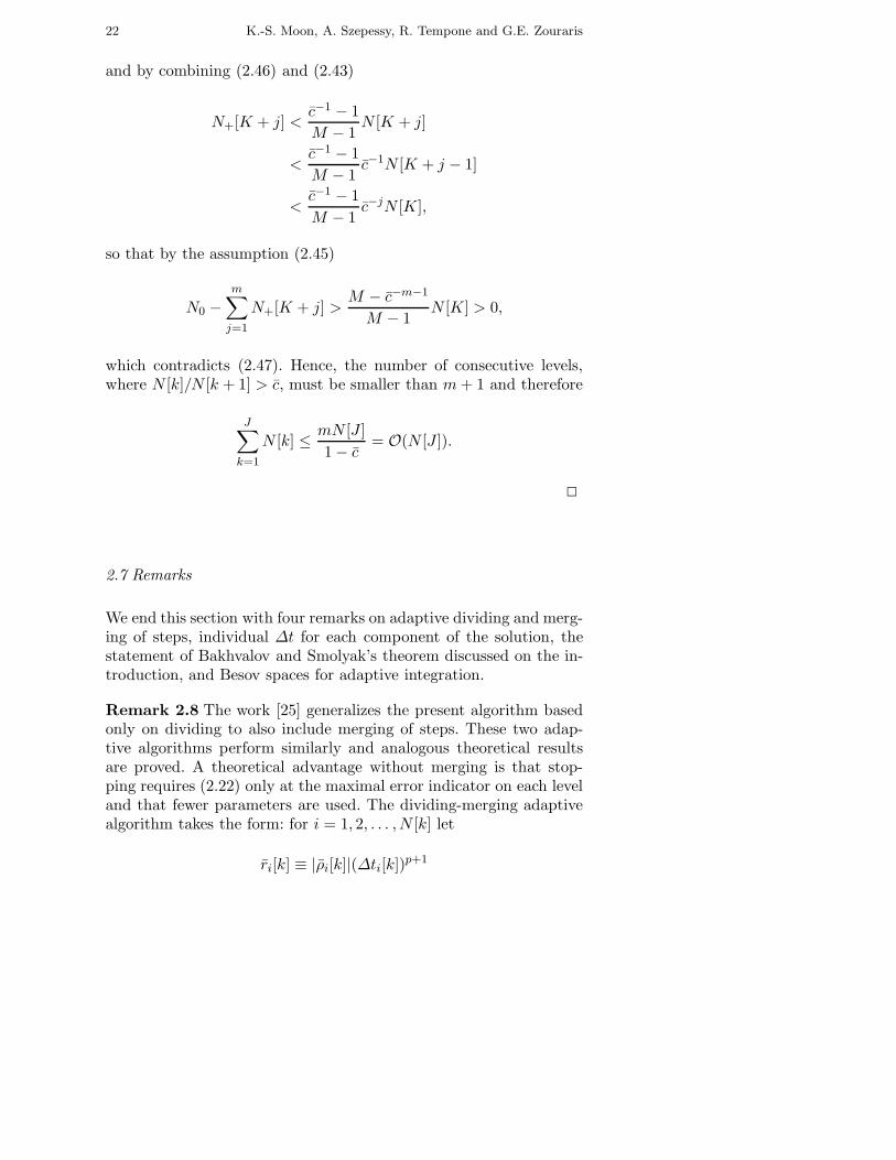
fig1.eps

Fig. 3.1. Example 3.1: Approximate X1-component from MSTZ with TOL =10−1.

We also compare the final number of time steps, Nf ≡ N [J ], and thetotal number of time steps, defined by

N tot ≡J∑

k=1

N [k], (3.2)

where J is the total number of refinement levels of MSTZ. Similarly,the total number of steps, N tot, for Uniform is the total sum of thenumbers of steps increasing a factor of 2 on each level, from the sameinitial number of step N [1], until Error ≤ TOL. Finally, the N tot forODE45 is the total sum of the numbers of steps with TOL decreasinga factor of 10, from the same TOL as MSTZ, until Error ≤ TOL.

We initialize MSTZ by setting s1 = 2 in (2.19), S1 = 2Ms1 by(2.23), and M = 2.

Example 3.1 Consider the well-known Lorenz system, which is thethree dimensional system of ordinary differential equations,

a1(t, x) = −σx1 + σx2,

a2(t, x) = rx1 − x2 − x1x3, 0 ≤ t ≤ T, x ∈ R3,

a3(t, x) = x1x2 − bx3

(3.3)

where σ , r and b are given positive constants.

The Lorenz system was introduced to show the limitation of largetime prediction for a simplified model of weather forecast, see [24]and Figure 3.1. In our experiments, the coefficient values are σ = 10,b = 8/3 and r = 28 and the initial value is X(0) = (1, 0, 0), cf. [7]and [16]. The computed function is g(x) = x1, i.e., we study the


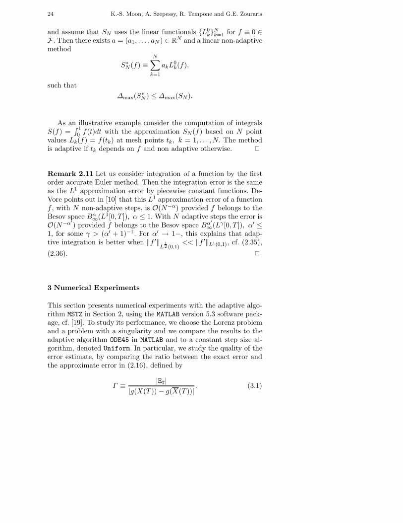
fig2.eps

fig3.eps

Fig. 3.2. Example 3.1: Comparison of the mesh functions of MSTZ and ODE45.The minimum value of Δt of MSTZ is 0.0016 which is 22 times larger than theminimum of ODE45.

global error |X1(T ) − X1(T )| at the final time T = 30. A referencecomputation with a Fortran implementation of MSTZ in quadrupleprecision gives the approximate value X1(30) � −3.892637 ≡ g1, withTOL = 10−7.

ODE45 is based on an explicit Runge-Kutta (5,4) formula, theDormand-Prince pair, see [11]. In order to compare with ODE45, theprogram MSTZ also uses the same 5-th order explicit Runge-Kuttamethod to compute X(tn+1), Ψ(tn) and X(tn+1). The approximatelocal “exact” solution X is computed with the half mesh size, i.e.,γ = 25/(25 − 1) in (2.7). The program Uniform uses a constant stepsize, Δt = constant, based on the same 5-th order explicit Runge-Kutta method. Table 1 and Figure 3.2 show that the algorithm MSTZ


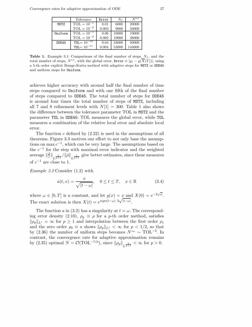
Tolerance Error Nf N tot

MSTZ TOL = 10−1 0.01 6000 20000TOL = 10−2 0.003 9000 34000

Uniform TOL = 10−1 0.06 10000 19000TOL = 10−2 0.002 19000 38000

ODE45 TOL= 10−10 0.04 34000 92000TOL= 10−11 0.004 53000 144000

Table 1. Example 3.1: Comparisons of the final number of steps, Nf , and thetotal number of steps, N tot, with the global error, Error ≡ |g1 − g(X(T ))|, usinga 5-th order explicit Runge-Kutta method with adaptive steps for MSTZ or ODE45

and uniform steps for Uniform.

achieves higher accuracy with around half the final number of timesteps compared to Uniform and with one fifth of the final numberof steps compared to ODE45. The total number of steps for ODE45is around four times the total number of steps of MSTZ, includingall 7 and 8 refinement levels with N [1] = 300. Table 1 also showsthe difference between the tolerance parameter TOL in MSTZ and theparameter TOL in ODE45: TOL measures the global error, while TOLmeasures a combination of the relative local error and absolute localerror.

The function c defined by (2.22) is used in the assumptions of alltheorems. Figure 3.3 motives our effort to not only base the assump-tions on max c−1, which can be very large. The assumptions based onthe c−1 for the step with maximal error indicator and the weightedaverage ‖ ρ

c‖L1

p+1/‖ρ‖

L1

p+1give better estimates, since these measures

of c−1 are close to 1.

Example 3.2 Consider (1.2) with

a(t, x) =x√|t − ω| , 0 ≤ t ≤ T, x ∈ R (3.4)

where ω ∈ [0, T ] is a constant, and let g(x) = x and X(0) = e−2√

ω.The exact solution is then X(t) = esign(t−ω) 2

√|t−ω|.

The function a in (3.2) has a singularity at t = ω. The correspond-ing error density (2.10), ρp ≡ ρ for a p-th order method, satisfies‖ρp‖L1 = ∞ for p ≥ 1 and interpolation between the first order ρ1

and the zero order ρ0 ≡ a shows ‖ρp‖L1 < ∞ for p < 1/2, so thatby (2.36) the number of uniform steps becomes N uni ∼ TOL−2. Incontrast, the convergence rate for adaptive approximation remainsby (2.35) optimal N = O(TOL−1/p), since ‖ρp‖

L1

p+1< ∞ for p > 0.


fig4.eps

Fig. 3.3. Example 3.1: Comparison between max c−1, the c−1 for the step withmaximal error indicator and the weighted average ‖ ρ

c‖

L1

p+1/‖ρ‖

L1

p+1. We see

that the last two are close to 1, while max c−1 is very large, which motivates theassumptions in the theorems.

fig5.eps

fig6.eps

Fig. 3.4. Example 3.2: Approximate solution (up) and mesh function (down)of MSTZ using a 5-th order explicit Runge-Kutta method with TOL = 10−4 andω = 5/3.


fig7.eps

Fig. 3.5. Example 3.2: The ratio of the approximate and exact error, Γ , convergesto 1 as TOL → 0+ with the stopping condition (2.20), while Γ does not convergeto 1 with the alternative stopping condition |ET| ≤ TOL. In general the condition|ET| ≤ TOL stops the program earlier and for some examples the error ratio Γ isnot as accurate as with the condition (2.20).

Consider the case ω = 5/3 with T = 4, N [1] = 25 and TOL =10−1, 10−4. Table 2 and Figure 3.4 show that MSTZ and ODE45 aremuch more efficient than Uniform, as expected.

Tolerance Error Nf N tot

MSTZ TOL = 10−1 0.02 50 820TOL = 10−4 2.6 × 10−5 130 3880

Uniform TOL = 10−1 0.06 130000 2600000.015 2100000 4200000

ODE45 TOL= 10−5 0.02 210 480TOL= 10−8 4.8 × 10−6 710 1800

Table 2. Example 3.2: Comparisons of the final number of steps, Nf , and thetotal number of steps, N tot, with the global error, Error ≡ |X(T )−X(T )|, usinga 5-th order explicit Runge-Kutta method with adaptive steps for MSTZ or ODE45

and uniform steps for Uniform. Adaptive approximation is more efficient for thissingularity.

Figure 3.5 compares stopping by (2.20) and the alternative |ET| ≤TOL. In general, the condition |ET| ≤ TOL stops the program earlierthan with the stopping condition (2.20) and sometimes this yields aless accurate error estimate as in Figure 3.5.


fig8.eps

Fig. 3.6. Example 3.1: The error indicators and the first component of theweights and the local errors from MSTZ with TOL = 10−1. The other two compo-nents have a similar behavior. Note that the local errors and the weights oscillate,but their product does not give a significant error cancellation, see Table 3.

Remark 3.3 If a time node, say tm+1, hits the singularity at t = ω,the approximation X(tm+1) becomes an infinite number. A rem-edy for this is to change the time steps, i.e tm := tm + α andtm+1 := tm+1 + β where α and β are sufficiently small numbers,e.g. Δtm/M , and then recompute X(tm) and X(tm+1). Using thistechnique, we solve Example 3.2 for w = 1 and T = 4 and we get|g(X(T )) − g(X(T ))| = 1.3065 × 10−4 with 113 final time steps and2567 total time steps using a 5-th order explicit Runge-Kutta methodand TOL = 10−3, N [1] = 40. �

Lorenz (Example 3.1) Singularity (Example 3.2)

Tolerance 10−1 10−2 10−1 10−4

Γ 0.991 0.997 1.325 2.31

Γ 1.707 1.220 1.325 2.66

Table 3. Example 3.1 and 3.2: Comparisons of the ratio, Γ and Γ , between theexact error and the approximate error using error density, ρ and |ρ| respectively,for MSTZ.

Remark 3.4 The algorithm MSTZ does not use the sign of the er-ror density. Therefore the computational error, ET ≡ ∑N

i=1 ρiΔtp+1i

in (2.16) could be much smaller than TOL ≥ (1/S1)∑N

i=1 |ρi|Δtp+1i ,


when it stops. Table 3 compares the quantities Γ in (3.1) and Γ ≡|∑N

i=1 |ρi|Δtp+1i |/|g(X(T )) − g(X(T ))| for the Examples 3.1 and 3.2.

Figure 3.6 shows the error indicators and the first component of theweights and the local errors in Example 3.1. We observe that thecancellation of the error in

∑Ni=1 ρiΔtp+1

i only yields a factor of tworeduction compared to

∑Ni=1 |ρi|Δtp+1

i . Therefore the time steps de-termined by the error bound

∑Ni=1 |ρi|Δtp+1

i , ignoring the sign andthe cancellation of the error, are also almost optimal taking cancel-lation into account, for these two examples. The cancellation of theerror is very important for Ito stochastic differential equations. In[33] we use properties of Brownian motion to derive an error densitywhich takes cancellation into account. �

Acknowledgements This work has been supported by the EU–TMR project HCL# ERBFMRXCT960033, the EU–TMR grant # ERBFMRX-CT98-0234 (Viscos-ity Solutions and their Applications), the Swedish Science Foundation, UdelaRand UdeM in Uruguay, the Swedish Network for Applied Mathematics, the Par-allel and Scientific Computing Institute (PSCI) and the Swedish National Boardfor Industrial and Technical Development (NUTEK).

References

1. M. Ainsworth and J. T. Oden, A posteriori error estimation in finite elementanalysis, Comput. Methods Appl. Mech. Engrg., 142 (1997), 1-88.

2. I. Babuska, A. Miller and M. Vogelius, Adaptive methods and error estima-tion for elliptic problems of structural mechanics, in Adaptive computationalmethods for partial differential equations ( SIAM, Philadelphia, Pa., 1983)57-73.

3. I. Babuska, and M. Vogelius, Feedback and adaptive finite element solutionof one-dimensional boundary value problems, Numer. Math. 44 (1984), no.1, 75-102.

4. N.S. Bakhvalov, On the optimality of linear methods for operator approxima-tion in convex classes of functions, USSR Comput. Math. and Math. Phys.,11 (1971), 244-249.

5. R. Becker and R. Rannacher, A feed-back approach to error control in finiteelement methods: basic analysis and examples, East-West J. Numer. Math.,4 (1996), no. 4, 237-264.

6. R. Becker and R. Rannacher, An optimal control approach to a posteriorierror estimation in finite element methods Acta Numerica, (2001), 1-102.

7. K. Bottcher and R. Rannacher, Adaptive error control in solving ordinarydifferential equations by the discontinuous Galerkin method, preprint, (1996).

8. A. Cohen, W. Dahmen and R. DeVore, Adaptive wavelet methods for ellipticoperator equations: convergence rates, Math. Comp., 70 (2001), no. 233,25-75.

9. G. Dahlquist and A. Bjork, Numerical Methods, (Prentice-Hall, 1974).


10. R. A. DeVore, Nonlinear approximation, Acta Numerica, (1998), 51-150.

11. J.R. Dormand and P.J. Prince, A family of embedded Runge-Kutta formulae,J. Comput. Appl. Math., 6 (1980), no. 1, 19–26.

12. W. Dorfler, A convergent adaptive algorithm for Poisson’s equation, SIAMJ. Numer. Anal. 33 (1996), no. 3, 1106-1124.

13. K. Eriksson, D. Estep, P. Hansbo and C. Johnson, Introduction to adaptivemethods for differential equations, Acta Numerica, (1995), 105-158.

14. D. Estep, A posteriori error bounds and global error control for approxima-tion of ordinary differential equations, SIAM J. Numer. Anal., 32 (1995),1-48.

15. D. Estep, D. Hodges and M. Warner, Computational error estimates andadaptive error control for a finite element solution of launch vehicle trajectroryproblems, SIAM J. SCI. COMPUT., 21 (2000), 1609-1631.

16. D. Estep and C. Johnson, The pointwise computability of the Lorenz system,Math. Models Methods Appl. Sci., 8 (1998), 1277-1305.

17. F. Gao, Probabilistic analysis of numerical integration algorithms, J. Com-plexity 7 (1991), no. 1, 58-69.

18. E. Harrier, S.P. Norsett and G. Wanner, Solving Ordinary Differential Equa-tions I, (Springer-Verlag, 1993).

19. D.J. Higham and N.J. Higham , Matlab Guide, (Society for Industrial andApplied Mathematics, 2000).

20. C. Johnson, Error estimates and adaptive time-step control for a class ofone-step methods for stiff ordinary differential equations, SIAM J. Numer.Anal., 25 (1988), 908-926.

21. C. Johnson and A. Szepessy, Adaptive finite element methods for conserva-tion laws based on a posteriori error estimates, Comm. Pure Appl. Math.,48 (1995), 199-234.

22. H. Lamba and A. M. Stuart, Convergence results for the MATLAB ODE23routine, BIT, 38 (1998), No. 4, 751-780.

23. A. Logg, Multi-adaptive Galerkin methods for ODEs, (Licentiate thesis, ISSN0347-2809, Chalmers University of Technology, 2001),

http://www.md.chalmers.se/Centres/Phi/preprints/index.html.24. E. N. Lorenz, Deterministic non-periodic flows, J. Atmos. Sci., 20 (1963),

130–141.25. K.-S. Moon, Convergence rates of adaptive algorithms for deterministic and

stochastic differential equations, (Licentiate thesis, ISBN 91-7283-196-0, RoyalInstitute of Technology, 2001), http://www.nada.kth.se/∼moon/paper.html.

26. K.-S. Moon, E. von Schwerin, A. Szepessy and R. Tempone, Convergence ratesfor adaptive finite element approximation of partial differential equations,work in progress.

27. K.-S. Moon, A. Szepessy, R. Tempone and G.E. Zouraris, Hyperbolic differen-tial equations and adaptive numerics, in Theory and numerics of differentialequations (Eds. J.F. Blowey, J.P. Coleman and A.W. Craig, Durham 2000,Springer Verlag, 2001).

28. K.-S. Moon, A. Szepessy, R. Tempone and G.E. Zouraris, A variational prin-ciple for adaptive approximation of ordinary differential equations, Numer.Math. (in press).

29. P. Morin, R. Nochetto and K.G. Siebert, Data oscillation and convergence ofadaptive FEM, SIAM J. Numer. Anal., 38 (2000), 466-488.

30. E. Novak, On the power of adaption, J. Complexity, 12 (1996), 199-237.


31. A.M. Stuart, Probabilistic and detereministic convergence proofs for softwarefor initial value problems, Numerical Algorithms, 14 (1997), 227-260.

32. A. Szepessy and R. Tempone, Optimal control with multigrid andadaptivity, Fifth World Congress on Computational Mechanics,http://wccm.tuwien.ac.at.

33. A. Szepessy, R. Tempone and G. E. Zouraris, Adaptive weak approximationof stochastic differential equations, Comm. Pure Appl. Math., 54 (2001),1169-1214.

34. G. Soderlind, Automatic control and adaptive time-stepping ANODE01 Pro-ceedings, Numerical Algorithms.

35. J.F. Traub and A.G. Werschulz, Complexity and Information, CambridgeUniversity Press, Cambridge, 1998.

36. T. Utumi, R. Takaki and T. Kawai, Optimal time step control for the nu-merical solution of ordinary differential equations, SIAM J. Numer. Anal.,33 (1996), 1644-1653.

37. A. G. Werschulz, The Computational Complexity of Differential and IntegralEquations, An Information-Based Approach, Oxford Mathematical Mono-graphs. Oxford Science Publications. The Clarendon Press, Oxford UniversityPress, New York, 1991.

convergence rates for adaptive approximation of ordinary

Documents