1 rates of convergence of performance gradient estimates using function approximation and bias in...
Post on 22-Dec-2015
220 views
TRANSCRIPT
1
Rates of Convergence of Performance Gradient Estimates Using Function
Approximation and Bias in Reinforcement Learning
Greg Grudic University of Colorado at Boulder
andLyle Ungar
University of [email protected]
2
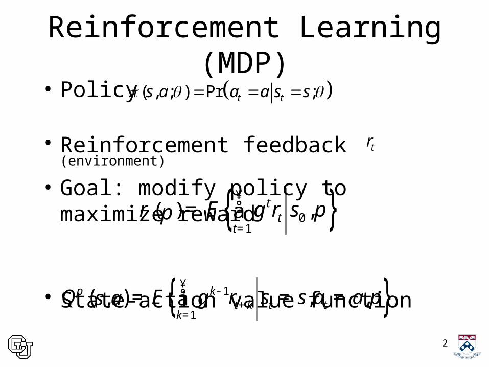
Reinforcement Learning (MDP)• Policy
• Reinforcement feedback (environment) • Goal: modify policy to maximize reward
• State-action value function
( , ; ) Pr ;t ts a a a s s
tr
( ) { }01
,tt
tE r sr g pp
¥
== å
( ) { }1
1, ,, k
t k t tk
Q E r s s a as ap g p¥
-+
== = =å

3
• Policy parameterized by –
• Searching space implies searching policy space
• Performance function implicitly depends on –
Policy Gradient Formulation
( , ; )s a
4
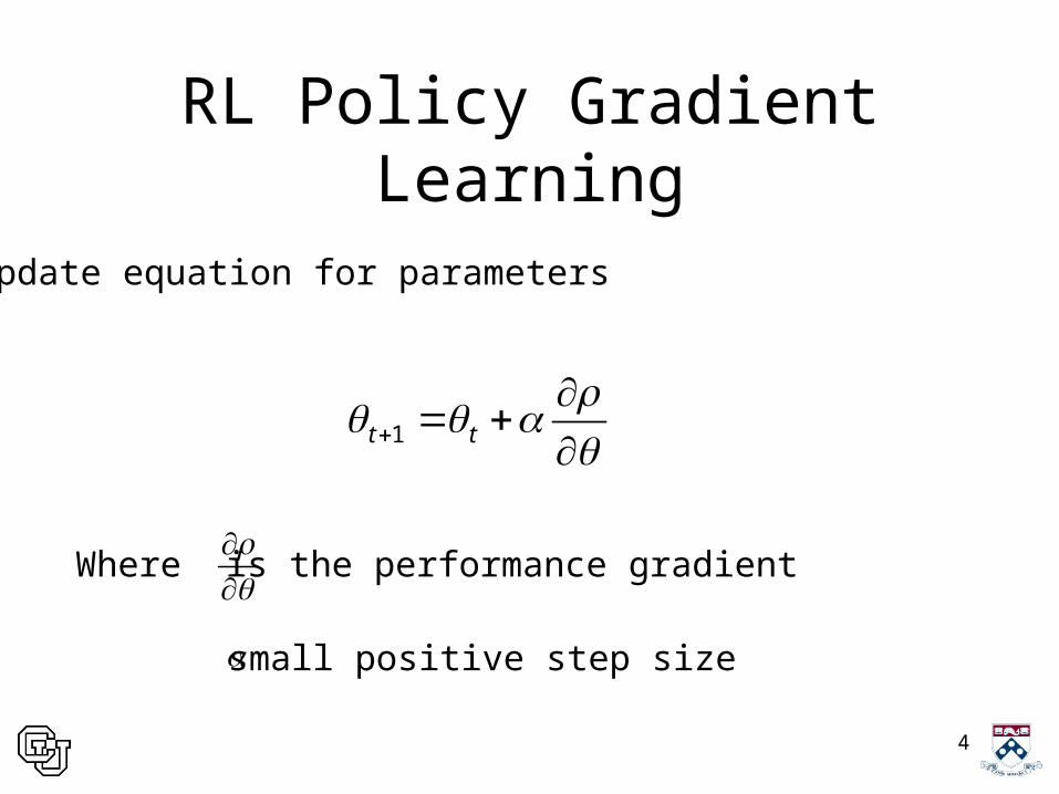
RL Policy Gradient Learning
1t t
Where is the performance gradient
Update equation for parameters
small positive step size
5
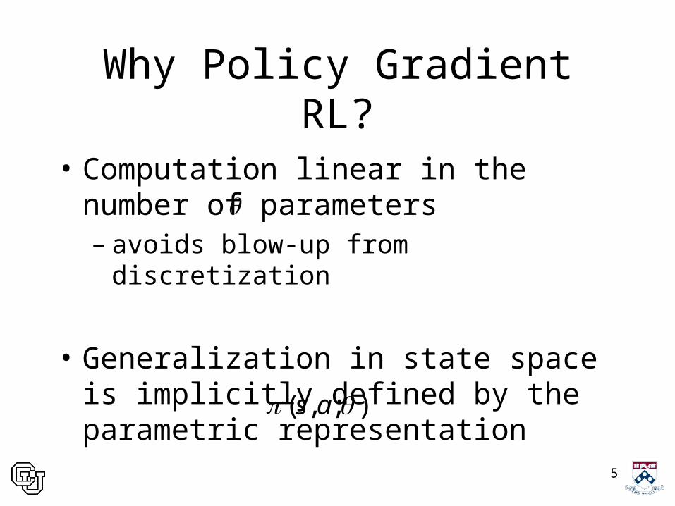
• Computation linear in the number of parameters – avoids blow-up from discretization
• Generalization in state space is implicitly defined by the parametric representation
Why Policy Gradient RL?
( , ; )s a
6
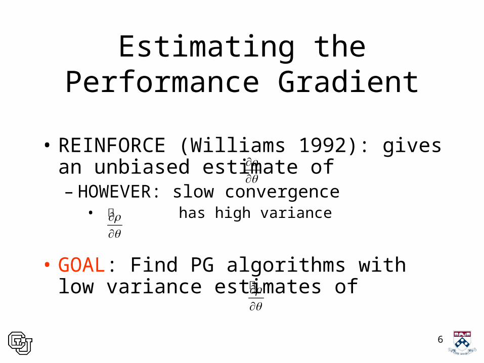
Estimating the Performance Gradient
• REINFORCE (Williams 1992): gives an unbiased estimate of– HOWEVER: slow convergence
• has high variance
• GOAL: Find PG algorithms with low variance estimates of
7
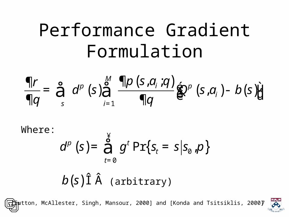
Performance Gradient Formulation
( )( )
( ) ( )1
, ;,
Mi
is i
s ad s Q s a b sp pp qr
q q=
¶¶ é ù= -ê úë û¶ ¶å å
( ) { }00
Pr ,tt
t
d s s s sp g p¥
=
= =å
( )b s Î Â
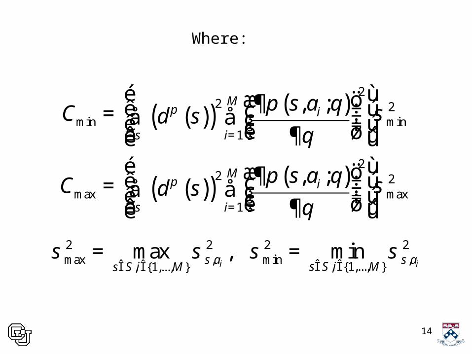
Where:
(arbitrary)
[Sutton, McAllester, Singh, Mansour, 2000] and [Konda and Tsitsiklis, 2000]
8
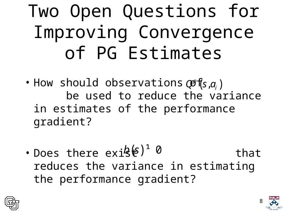
Two Open Questions for Improving Convergence of PG
Estimates
• How should observations of be used to reduce the variance in estimates of the performance gradient?
• Does there exist that reduces the variance in estimating the performance gradient?
( ), iQ s ap
( ) 0b s ¹
9
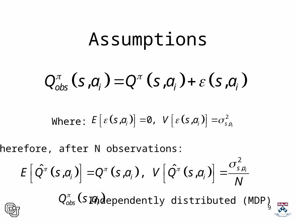
Assumptions
, , ,obs i i iQ s a Q s a s a
2,, 0, ,ii i s aE s a V s a
2,ˆ ˆ, , , , is a
i i iE Q s a Q s a V Q s aN
Where:
Therefore, after N observations:
,obs iQ s aIndependently distributed (MDP)
10
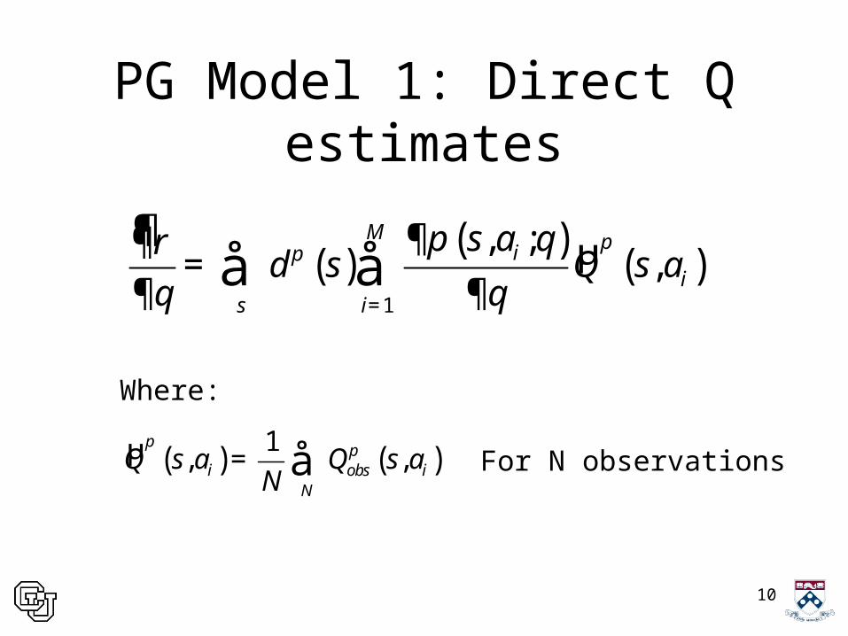
PG Model 1: Direct Q estimates
¶( )
( )µ ( )1
, ;,
Mi
is i
s ad s Q s a
pp p qrq q=
¶¶=
¶ ¶å å
µ ( ) ( )1, ,i obs i
N
Q s a Q s aN
p p= å For N observations
Where:
11
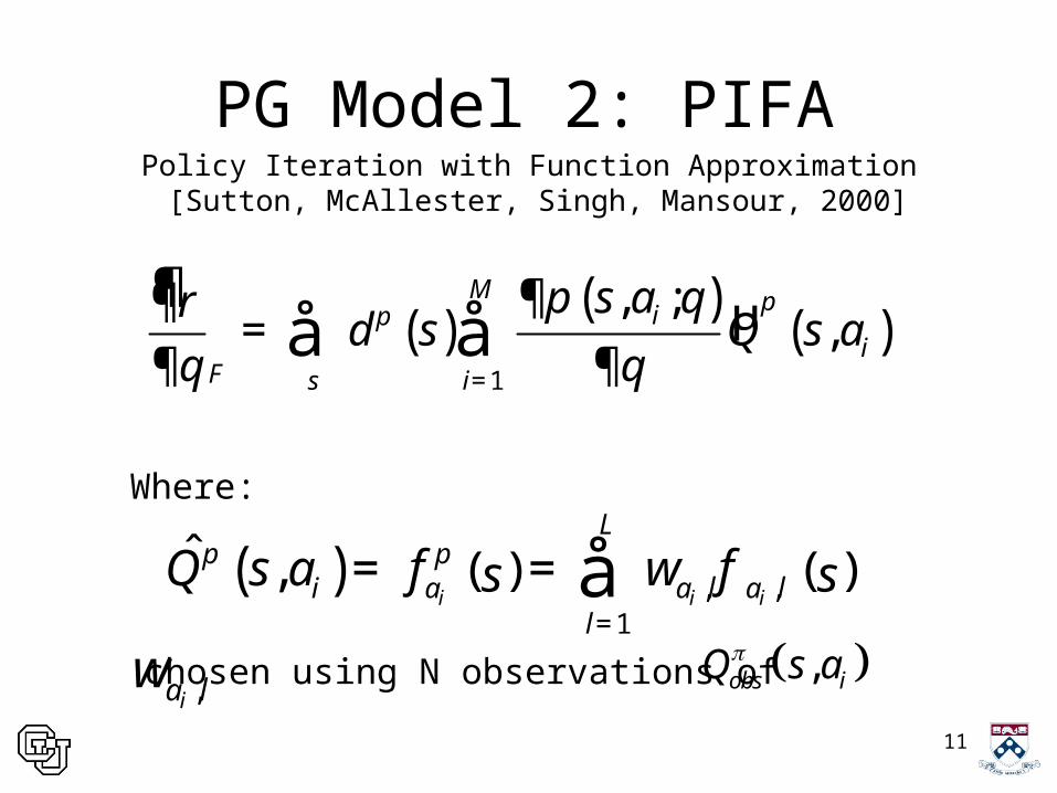
PG Model 2: PIFA
¶( )
( )µ ( )1
, ;,
Mi
iF s i
s ad s Q s a
pp p qrq q=
¶¶=
¶ ¶å å
chosen using N observations of
Policy Iteration with Function Approximation [Sutton, McAllester, Singh, Mansour, 2000]
( ) ( ) ( ), ,1
ˆ ,i i i
L
i a a l a ll
Q s a f ws sp p f
=
= =å,ia l
w ,obs iQ s a
Where:
12
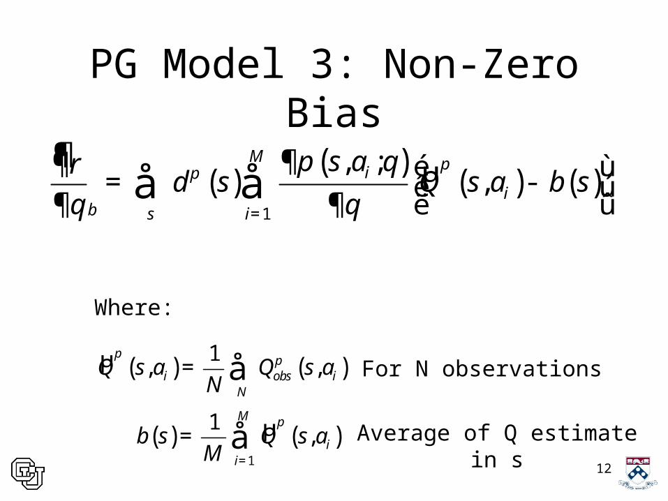
PG Model 3: Non-Zero Bias
¶( )
( ) µ ( ) ( )1
, ;,
Mi
ib s i
s ad s Q s a b s
pp p qrq q=
¶¶ é ù= -ê ú¶ ¶ ë ûå å
µ ( ) ( )1, ,i obs i
N
Q s a Q s aN
p p= å For N observations
Where:
( ) µ ( )1
1,
M
ii
b s Q s aM
p
=
= å Average of Q estimatein s
13
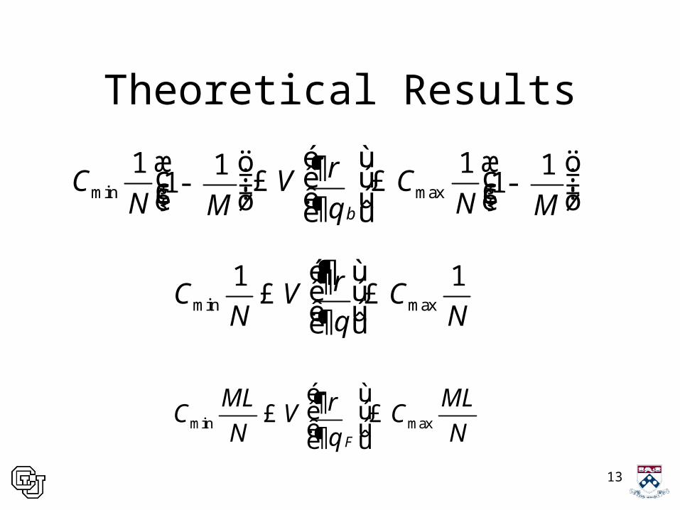
Theoretical Results
·min max
F
ML MLC V C
N Nrq
é ù¶ê ú£ £ê ú¶ë û
¶min max
1 1C V C
N Nrq
é ù¶ê ú£ £ê ú¶ë û
·min max
1 11 11 1
b
C V CN NM M
rq
é ùæ ö æ ö¶÷ ÷ç çê ú£ £- -÷ ÷ç ç÷ ÷ç çê úè ø è ø¶ë û
14
2 2 2 2max , min ,
, {1,..., }, {1,..., }max , min
i is a s as S i Ms S i M
s s s sÎ ÎÎ Î
= =
( )( ) ( )
( )( ) ( )
22 2
min min1
22 2
max max1
, ;
, ;
Mi
s i
Mi
s i
s aC d s
s aC d s
p
p
p q sq
p q sq
=
=
é ùæ ö¶ê ú÷ç= ÷å å çê ú÷÷ççè øê ú¶ë ûé ùæ ö¶ê ú÷ç= ÷å å çê ú÷÷ççè øê ú¶ë û
Where:
15
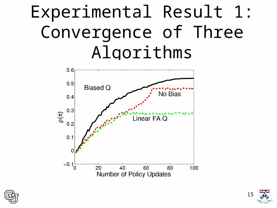
Experimental Result 1: Convergence of Three Algorithms
16
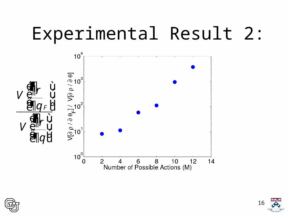
Experimental Result 2:
¶F
V
V
rq
rq
é ù¶ê úê ú¶ë ûé ù¶ê úê ú¶ë û

17
Experimental Result 3:
b
V
V
rqrq
é ù¶ê úê ú¶ë ûé ù¶ê úê ú¶ë û
18
Conclusion
• Implementation of PG algorithms significantly affects convergence
• Linear basis function representations of Q can substantially degrade convergence
• Appropriately chosen bias terms can improve convergence