convergence analysis and a dc approximation method … · 2019-11-07 · 1 convergence analysis and...

CONVERGENCE ANALYSIS AND A DC APPROXIMATION1

METHOD FOR DATA-DRIVEN MATHEMATICAL PROGRAMS2

WITH DISTRIBUTIONALLY ROBUST CHANCE CONSTRAINTS∗3

HAILIN SUN† , DALI ZHANG‡ , AND YANNAN CHEN§4

Abstract. In this paper, we consider the convergence analysis of data-driven mathematical5programs with distributionally robust chance constraints (MPDRCC) under weaker conditions with-6out continuity assumption of distributionally robust probability functions. Moreover, combining7with the data-driven approximation, we propose a DC approximation method to MPDRCC without8some special tractable structures. We also give the convergence analysis of the DC approximation9method without continuity assumption of distributionally robust probability functions, and apply a10recent DC algorithm to solve them. The numerical tests verify the theoretical results and show the11effectiveness of the data-driven approximated DC approximation method.12

Key words. Distributionally robust optimization, chance constraints, data-driven, convergence13analysis, DC approximation14

AMS subject classifications. 90C1515

1. Introduction. In this paper, we consider the mathematical programs with16

distributionally robust chance constraints (MPDRCC)17

(1)minx∈X

f(x)

s.t. infP∈P

P (g(x, ξ) ≤ 0) ≥ 1− α,18

and its data-driven formulation19

(2)minx∈X

f(x)

s.t. infP∈PN

P (g(x, ξ) ≤ 0) ≥ 1− α,20

where X is a closed subset of IRn, ξ : Ω → Ξ ⊂ IRk is a random vector defined on21

measurable space (Ω, F ) with support set Ξ, f : IRn → IR is Lipschitz continuous22

function w.r.t. x, g : IRn × IRk → IR is Lipschitz continuous function w.r.t. x for all23

ξ ∈ Ξ, P(Ξ) denotes the set of all probability measures defined on Ξ, P ⊂ P(Ξ) is24

the ambiguity set which indicates ambiguity of the true probability distribution of ξ25

and PN ⊂P(Ξ) is a set of probability measures which approximates P in some sense26

(to be specified later) as N →∞. In the case when the ambiguity set P is singleton,27

the problem reduces to mathematical programs with chance constraints (MPCC)28

(3)minx∈X

f(x)

s.t. P (g(x, ξ) ≤ 0) ≥ 1− α29

∗Submitted to the editors DATE.Funding: This work was funded by National Natural Science Foundation of China #11871276,

#11571056, #11571178 and #11771405. The authors certify that the general content of themanuscript, in whole or in part, is not submitted, accepted, or published elsewhere, including con-ference proceedings. The authors also certify that the general content of the manuscript, in whole orin part, will not be submitted, accepted, or published elsewhere, including conference proceedings,while it is under consideration or in production.†Corresponding author. Jiangsu Key Laboratory for NSLSCS, School of Mathematical Sciences,

Nanjing Normal University, Nanjing, 210023, China ([email protected]).‡Antai College of Economic and Management(SUGLI), Shanghai Jiao Tong University, 200030,

Shanghai, China, ([email protected]).§School of Mathematical Sciences, South China Normal University, Guangzhou, 510631, China,

([email protected])

1

This manuscript is for review purposes only.

mailto:[email protected]



2 HAILIN SUN, DALI ZHANG, YANNAN CHEN

and EP [1g(x,ξ)≤0(g(x, ξ))] = P (g(x, ξ) ≤ 0) where

1g<0(g) =

1 g < 00 g ≥ 0

is the index function.30

The MPCC has wide applications in engineering design, supply chain manage-31

ment, production planing, and water management, see [34]. MPCC was first dis-32

cussed by Charnes, Cooper, and Symonds [3], and then by Miller and Wagner [23]33

and Prekopa [27]. In recent years, there are many significant progress of MPCC34

from both a theoretical viewpoint and an algorithmic perspective. The convexity of35

chance constraints has been investigated by Henrion and Strugarek [14] and van Ack-36

ooij [38]. Under multivariate Gaussian distribution of random vector, van Ackooij37

and Henrion [39] propose an efficient method to compute the gradient and value of38

probability functions and then MPCC can be solved by existing solvers. Many ap-39

proximation methods also proposed for solving MPCC such as sample approximation40

[22], constrained bundle method and other methods with regularization [6], inner-41

outer approximation[9], convex approximation [24], difference of two convex function42

(DC) approximation [15, 17, 32], sample average approximation (SAA) [25]. For more43

discussion on MPCC, we refer readers to [28, 34] and references therein.44

In the case when the decision makers do not have full knowledge of the underlying45

probability distribution but still can obtain some partial information and use them to46

construct an ambiguity set of probability distributions which contains or approximates47

the true probability distribution, they may consider solving the MPDRCC. MPDRCC48

are important problems in distributionally robust optimization, a number of papers49

have appeared on this topic. In the case when the ambiguity set is characterized by its50

mean and variance and g(·, ·) has some special structures, Calafiore and El Ghaoui [2],51

Zymler, Kuhn, and Rustem [45] and Yang and Xu [43] prove that the MPDRCC can be52

tractable. Hanasusanto et al. [12] and Hanasusanto et al. [13] investigate tractability53

of a rich class of ambiguity sets defined through moment conditions and structural54

information for MPDRCC. In [42], Xie and Ahmed generalize the results in [2, 43, 45]55

and identified several sufficient conditions for convex reformulation of MPDRCC when56

ambiguity set is specified by moment constraints. Erdogan and Iyengar [7] construct57

an ambiguity set based on the Prohorov-metric and approximate MPDRCC by a set58

of sample-based robust optimization constraints. Jiang and Guan [18] and Hu and59

Hong [16] derive tractable reformulations for the family of φ-diverge probability metric60

(e.g., Kullback-Leibler (KL) divergence, Hellinger distance, etc.). Xie [40], Xie and61

Ahmed [41] and Chen et al. [5] investigate convex reformulation of MPDRCC with62

Wasserstein distance. However, in general cases, the MPDRCC are still intractable63

and difficult to solve.64

Our motivation starts from the convergence analysis of data-driven MPDRCC65

recently proposed by Guo et al. [11]. They consider the convergence analysis between66

(1) and (2) when PN converges to P under a key assumption:67

(4) infP∈P

P (g(x, ξ) ≤ 0) is continuous w.r.t. x.68

The continuity of the (distributional robust) probability functions is well documented69

in the literature of stochastic programming, see [11, 25, 37]. One sufficiently condition70

of (4) is71

(5) Pg(x, ξ) = 0 = 0 for all x ∈ X, ∀P ∈ P.72


CONVERGENCE ANALYSIS AND A DC APPROXIMATION METHOD FOR MPDRCC 3

Guo et al. [11] consider a weaker condition73

(6) PH(x)/int(H(x)) = 0 for all x ∈ X and P ∈ P,74

to guarantee (4), where H(x) := ξ : g(x, ξ) ≤ 0. However, for a large class of75

ambiguity sets, (5) and (6) can not be satisfied. Moreover, from the motivated example76

in Section 2.1 (Example 2.1), it seems that when (4) is not satisfied, the convergence77

may still holds. This motivates us to investigate the convergence analysis of MPDRCC78

under weaker conditions without (4).79

We also interesting in how to solve the data-driven MPDRCC. Different from80

tractable reformulation base on the special structure of MPDRCC in the literatures,81

we consider a DC approximation of MPDRCC which is inspired by the DC approxi-82

mation proposed in Hong et al. [15] for MPCC. In [15], Hong et al. use condition83

(7) Pg(x, ξ) = 0 = 0 for all x ∈ X84

to guarantee the continuous assumption (4) and proof the convergence of DC approx-85

imation. Hu et al. [17] relax the condition (7) by using smoothing method. But they86

still require87

(8) x : Pg(x, ξ) > 0 ≤ α = clx : Pg(x, ξ) > 0 < α.88

By slightly changing their approach, we propose a different DC approximation which89

does not require condition (7) or (8), and apply the approach to MPDRCC. The90

contributions of the paper are as follows:91

(i) We study the data-driven MPDRCC and corresponding convergence analysis.92

This part can be considered as an extention of resent work by Guo et al. [11]93

but under weaker conditions without the continuity assumption (4).94

(ii) Moreover, for solving MPDRCC without tractable structures, we propose95

a DC approximation method for MPDRCC. The DC approximation method96

can be considered as an extension of DC approximation of MPCC in [15]. The97

convergence analysis has been investigated under weaker conditions without98

continuity assumption of probability functions. We also study the conver-99

gence analysis of data-driven DC approximated MPDRCC.100

(iii) With three kinds of ambiguity sets, we reformulate the data-driven DC ap-101

proximated MPDRCC as optimization problems with DC constraints and102

apply the penalty and augmented Lagrangian methods proposed by Lu et.103

al. [21] to solve them. The numerical tests show that the correctness of our104

theoretical results and effectiveness of the DC approximation.105

The paper is constructed as follows. Some preliminarise knowledge and a mo-106

tivation example are given in Section 2. In Section 3, we study the data-driven107

MPDRCC and the corresponding convergence analysis without continuity condition108

(4). In Section 4, we propose a DC approximation of MPDRCC and investigate the109

convergence analysis. In Section 5, we reformulate the DC approximated MPDRCC110

as optimization problems with DC constraints under three kinds of ambiguity sets.111

The the penalty and augmented Lagrangian methods proposed by Lu et al. [21] has112

been applied to solve the optimization problems with DC constraints. Elementary113

numerical tests and applications are given in Section 6 to show the correctness of the114

theorems and the effectiveness of the DC approximation.115

Throughout the paper, we use the following notation. IRn+ denotes the cone of116

vectors with non-negative components in IRn. P(Ξ) denotes the set of all probability117

measures over Ξ. For a set C ⊂ Z, we use by convention “int C” and “cl C” to denote118

its interior and closure respectively.119



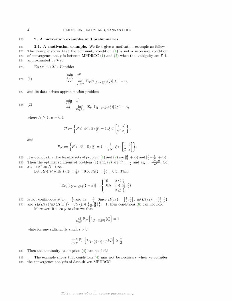
2. A motivation examples and preliminaries .120

2.1. A motivation example. We first give a motivation example as follows.121

The example shows that the continuity condition (4) is not a necessary condition122

of convergence analysis between MPDRCC (1) and (2) when the ambiguity set P is123

approximated by PN .124

Example 2.1. Consider125

(1)minx∈X

x2

s.t. infP∈P

EP [1ξ−x≤0(ξ)] ≥ 1− α,126

and its data-driven approximation problem127

(2)minx∈X

x2

s.t. infP∈PN

EP [1ξ−x≤0(ξ)] ≥ 1− α,128

where N ≥ 1, α = 0.5,

P :=

P ∈P : EP [ξ] = 1, ξ ∈

[1

2,

3

2

],

and

PN :=

P ∈P : EP [ξ] = 1− 1

2N, ξ ∈

[1

2,

3

2

].

It is obvious that the feasible sets of problem (1) and (2) are [ 32 ,+∞) and [ 3

2−1N ,+∞).129

Then the optimal solutions of problem (1) and (2) are x∗ = 32 and xN = 3N−2

2N . So130

xN → x∗ as N →∞.131

Let P0 ∈ P with P0(ξ = 12 ) = 0.5, P0(ξ = 3

2 ) = 0.5. Then

EP0[1ξ−x≤0(ξ − x)] =

0 x ≤ 12

0.5 x ∈ ( 12 ,

32 )

1 x ≥ 32

is not continuous at x1 = 12 and x2 = 3

2 . Since H(x1) =[

12 ,

32

], intH(x1) =

(12 ,

32

)132

and P0H(x)/int(H(x)) = P0

ξ ∈

12 ,

32

= 1, then conditions (6) can not hold.133

Moreover, it is easy to observe that

infP∈P

EP[1ξ− 3

2≤0(ξ)]

= 1

while for any sufficiently small ε > 0,

infP∈P

EP[1ξ−( 3

2−ε)≤0(ξ)]≤ 1

2.

Then the continuity assumption (4) can not hold.134

The example shows that conditions (4) may not be necessary when we consider135

the convergence analysis of data-driven MPDRCC.136



2.2. Graphical convergence and metrics of probability measures. Let137

N = 1, 2 . . . be the set of natural numbers, N#∞ = all subsequences of N and138

N∞ = all indexes ≥ some k. For sequence N , we use (xk, εk) −→N

(x, 0) to denote139

εk ↓ 0 and xk → x when k ∈ N .140

Definition 1. [31, Definition 5.32] For the mappings zε : X → IRn+1, the graph-141

ical outer limit, denoted by g- lim supε zε : X ⇒ IRn+1, is the mapping having as its142

graph the set lim supε gphzε:143

g- lim supε zε(x) = z | ∃N ∈ N#

∞, (xk, εk)−→N

(x, 0), zεk(xk)−→Nz.144

The graphical inner limit, denoted by g- lim infε zε, is the mapping having as its graph

the set lim infε gphzε:

g- lim infε zε(x) = z | ∃N ∈ N∞, (xk, εk)−→

N(x, 0), zεk(xk)−→

Nz.

If the outer and inner limits coincide, the graphical limit g- limε zε exists; thus, Z0 =145

g- limε zε if and only if g- lim supε z

ε ⊆ Z0 ⊆ g- lim infε zε and one writes zε

g−→ Z0;146

the mappings zε are said to converge graphically to Z0.147

Metrics of probability measures: We need appropriate metrics for the set148

in order to characterize convergence of PN → P. In this section, we will introduce149

ζ-metrics and pseudometric, see [1, 10].150

Definition 2. A (semi-) ζ-metric is defined by151

(3) dlG (P,Q) := supg∈G|EP [g(ξ)]− EQ[g(ξ)]| ,152

where P,Q ∈P(Ξ) and G is a set of real-valued bounded measurable functions on Ξ.153

The ζ-metrics cover a wide range of metrics in probability theory including the to-154

tal variation metric, Kantorovich/ Wasserstein metric, bounded Lipschitz metric and155

some other metrics; see [10], [29] or [44] and references therein. Specifically, if156

G :=

g : Ξ→ R| g is B measurable, sup

ξ∈Ξ|g(ξ)| ≤ 1

,157

then dlG reduces to the total variation metric, denoted by dlTV . If g is restricted158

further to be Lipschitz continuous with modulus bounded by 1, that is,159

G = g : g is Lipschitz continuous and Lipschtiz modulus L1(g) ≤ 1 ,160

then we arrive at Kantorovich/ Wasserstein metric, denoted by dlK .161

Under the ζ-metric dlG , we can define the distance from a distribution Q to a162

set of distributions C as dlG (Q, C) := infP∈C dlG (Q,P ), deviation from one set C ∈163

P(Ξ) to another C′ ∈ P(Ξ) as D(C′, C; dlG ) := supQ∈C′ dlG (Q, C) and the Hausdorff164

distance between two subset C and C′ in the space of probability measures P(Ξ) as165

H(C′, C; dlG ) := max D(C′, C; dlG ), D(C, C′; dlG ) .166

In the case when the set of function G is not large enough such that

supg∈G

∣∣EP [g]− EQ[g]∣∣ = 0

does not necessarily imply P = Q, the type of “metric” is not a ζ-metric, and named167

by pseudometric. This type of pseudometric is widely used for stability analysis in168

stochastic programming; see an excellent review by Romisch [30].169

We also introduce two definitions from [1]:170



Definition 3. Let A be a set of probability measures on (Ξ,B). A is said to be171

tight if for any ε > 0, there exists a compact set Ξε ⊂ Ξ such that infP∈A P (Ξε) > 1−ε.172

In the case when A is a singleton, it reduces to the tightness of a single probability173

measure. A is said to be closed (under the weak topology) if for any sequence PN ⊂174

A with PN → P weakly, we have P ∈ A.175

Definition 4. Let PN ⊂ P be a sequence of probability measures. PN is176

said to converge to P ∈P weakly if limN→∞∫

Ξh(ξ)PN (dξ) =

∫Ξh(ξ)P (dξ) for each177

bounded and continuous function h : Ξ → IR. Let A ⊂ A be a set of probability178

measures. A is said to be weakly compact (under the weak topology) if every sequence179

AN ⊂ A contains a subsequence AN ′ and A ∈ A such that AN ′ → A.180

3. Convergence analysis in data-driven problem. In this section, we con-181

sider the equivalent formulation of problem (1):182

(1)minx∈X

f(x)

s.t. supP∈P

EP [1g(x,ξ)>0(ξ)] ≤ α,183

and its data-driven form:184

(2)minx∈X

f(x)

s.t. supP∈PN

EP [1g(x,ξ)>0(ξ)] ≤ α.185

In what follows, we consider the convergence of the optimal solution sets of (2).186

To ease the exposition, for each fixed x ∈ X, let187

(3) v(x) := supP∈P

EP[1(g(x,ξ)>0)

], vN (x) := sup

P∈PNEP[1(g(x,ξ)>0)

],188

F∗, ϑ∗, S∗ and FN , ϑN , SN be the feasible solution set, the optimal value and the189

optimal solution set of problem (1) and (2) respectively. Let P ⊂ P denote a set of190

distributions such that191

(4) P,PN ⊂ P192

for N sufficiently large. The existence of P is trivial as we can take the union of P193

and PN , for N = 1, 2, 3, · · · .194

Assumption 3.1. Let P,PN be nonempty and defined as in (1) and (2) respec-195

tively. Then196

(a) there exists a weakly compact set (see Definition 4) P ⊂ P such that (4)197

holds;198

(b) H(PN ,P; dlL1)→ 0 almost surely as N →∞, where H(·, ·; dlL1) is defined as199

in Section 2.2 with G1 := l(·) = 1g(x,ξ)>0(ξ) : x ∈ X.200

In [11, Theorem 3.2], Guo et. al. investigate the convergence analysis between201

vN and v under Assumption 3.1 and the assumption can hold in several cases, e.g.,202

H(PN ,P; dlTV )→ 0, see [35].203

Proposition 3.1. [11, Theorem 3.2] Suppose Assumption 3.1 (b) holds, then204

vN (·) converges uniformly to v(·) over X as N tends to infinity, that is,205

(5) limN→∞

supx∈X|vN (x)− v(x)| = 0.206

207



To avoid assuming continuity of v(·), we proof the lower semi-continuity of v(·).208

Lemma 3.1. Suppose Assumption 3.1 (a) holds and g(x, ξ) is continuous w.r.t. x209

for all ξ ∈ Ξ, then the function v(·) defined in (3) is lower semi-continuous.210

Proof. Note that g(·, ξ) is continuous for all ξ ∈ Ξ, it is easy to observe that211

1g(x,ξ)>0(g(x, ξ)) is lower semi-continuous w.r.t. x for all ξ ∈ Ξ.212

Let xk be any sequence that converges to x. Then213

lim infk→∞

v(xk)− v(x) = lim infk→∞

(v(xk)− v(x))214

= lim infk→∞

(supP∈P

EP [1g(xk,ξ)>0(g(xk, ξ))]− supP∈P

EP [1g(x,ξ)>0(g(x, ξ))]

).(6)215

Note that for any P0 ∈ P,

supP∈P

EP [1g(xk,ξ)>0(g(xk, ξ))]− supP∈P

EP [1g(x,ξ)>0(g(x, ξ))]

≥ EP0[1g(xk,ξ)>0(g(xk, ξ))]− sup

P∈PEP [1g(x,ξ)>0(g(x, ξ))].

Moreover, for any ε > 0, there exists Pε ∈ P such that

supP∈P

EP [1g(x,ξ)>0(g(x, ξ))] ≤ EPε [1g(x,ξ)>0(g(x, ξ))] + ε.

Then216

(7)supP∈P

EP [1g(xk,ξ)>0(gxk, ξ))]− supP∈P

EP [1g(x,ξ)>0(g(x, ξ))]

≥ EPε [1g(xk,ξ)>0(g(xk, ξ))]− EPε [1g(x,ξ)>0(g(x, ξ))]− ε.217

Combine (6) and (7) and by Fatou’s Lemma and the lower semi-continuous of218

1g(x,ξ)≥0(g(x, ξ)) w.r.t. x for all ξ ∈ Ξ, we have219

lim infk→∞

v(xk)− v(x) ≥ lim infk→∞

EPε[1g(xk,ξ)>0(g(xk, ξ))− 1g(x,ξ)>0(g(x, ξ))

]− ε220

≥ EPε[lim infk→∞

(1g(xk,ξ)>0(g(xk, ξ))− 1g(x,ξ)>0(g(x, ξ))

)]− ε ≥ −ε221

Moreover, by the arbitrariness of ε, lim infk→∞ v(xk) − v(x) ≥ 0 for any sequence222

xk → x as k →∞, and then v(·) is lower semi-continuous w.r.t. x.223

Now we are ready to prove the convergence of data-driven MPDRCC, the main224

result in the section.225

Theorem 3.1. Assume that X is a compact set, S∗ and SN are nonempty for226

sufficiently large N > 0. Suppose (a) g(x, ξ) is continuous w.r.t. x for all ξ ∈ Ξ, (b)227

clFs ∩ S 6= ∅, where Fs := x ∈ X : v(x) < α, (c) Assumption 3.1 holds. Then we228

have (i) limN→∞

ϑN = ϑ∗; (ii) limN→∞

D(SN ,S∗) = 0.229

Proof. Let xN be any sequence of optimal solutions of problem (2) and x∗230

be any accumulation point. Then without loss of generality, there exists a subse-231

quence Nk such that xNk is the subsequence of the solutions of problem (2) and232

limk→∞ xNk = x∗. By the continuity of the objective function f , we only need to233

prove x∗ ∈ S∗.234



We prove the feasibility of x∗ for problem (1) firstly. Note that xNk ∈ SNk ,235

vNk(xNk) ≤ α. Moreover, vN (·) converges to v(·) uniformly, then for any δ1 > 0,236

there exists k0 > 0 such that237

(8) supx∈X|vNk(x)− v(x)| ≤ δ1238

for all k ≥ k0. Then for any δ1 > 0, there exists k0 > 0 such that v(xNk) ≤ α + δ1239

for all k ≥ k0. Furthermore, by Lemma 3.1, v(·) is lower semi-continuous, then for all240

k ≥ k0, v(x∗) ≤ lim infk→∞ v(xNk) ≤ α + δ1. By the arbitrariness of δ1, v(x∗) ≤ α,241

which implies x∗ ∈ F .242

Then we consider Fδ := x ∈ X : v(x) ≤ α− δ with δ > 0 and problem243

ϑδ := minx∈Xf(x) s.t. x ∈ Fδ.(9)244

Let xδ be any sequence of optimal solutions of problem (9). By condition (b), we245

have limδ↓0 Fδ = clFs, then any accumulation point of the sequence x ∈ S. By (8),246

for any δ > 0, there exists sufficiently large kδ such that Fδ ⊆ FNkδ and Nkδ is a247

subsequence of Nk. Then we have xNkδ → x∗ and f(xNkδ ) ≤ f(xδ), which implies248

f(x∗) ≤ f(x) = ϑ∗. Combining this inequation with x∗ ∈ F , we have x∗ ∈ S∗.249

Condition (b) in Theorem 3.1 requires problem (1) to have a non-isolated optimal250

solution. It is fulfilled if the feasible set F is convex or connected and discussed in [11,251

Theorem 3.4]. Moreover, the following example shows when condition (b) in Theorem252

3.1 fails, the convergence can not hold.253

Example 3.1. Consider254

(10)minx∈X

x2

s.t. supP∈P

EP [1ξ−x>0(ξ)] ≤ α,255

and its approximation problem256

(11)minx∈X

x2

s.t. supP∈PN

EP [1ξ−x>0(ξ)] ≤ α,257

where

P =

P ∈P(Ξ) :

Probξ = −1 = 0.25, Probξ = 0 = 0.25,Probξ = 1 = 0.25, Probξ = 2 = 0.25

and

PN =

P ∈P(Ξ) :

Probξ = −1 = 0.25− 1N , Probξ = 0 = 0.25,

Probξ = 1 = 0.25 + 1N , Probξ = 2 = 0.25

,

N ≥ 4, α = 0.5 and Ξ := −1, 0, 1, 2. It is obvious that the feasible sets of problem258

(10) and (11) are [0,+∞) and [1,+∞). Then the optimal solutions of problem (10)259

and (11) are x∗ = 0 and xN = 1 respectively. So xN 9 x∗ as N →∞.260

4. DC approximation methods of MPDRCC. In the literatures, there are261

several tractable reformulation of MPDRCC when the problems satisfy some special262

structures. But in general cases, the MPDRCC are intractable. In this section, we263

consider a DC approximation method for general MPDRCC.264



4.1. DC Approximation Methods. We consider the DC approximation of265

index function as follows:266

Definition 4.1. The DC approximation function of index function 1·>0(·), de-267

note by ΨDC(·, ε), is defined as268

(1) ΨDC(·, ε) :=1

ε((·)+ − (· − ε)+) ,269

where ε > 0.270

Lemma 4.1. The DC approximation function ΨDC(·, ε) of index function 1·>0(·)271

is globally Lipschitz continuous and increaseing w.r.t. · for any ε > 0 such that,272

(1). ΨDC(·, ε) pointwise converges to 1·>0(·);273

(2). ΨDC(·, ε) g−→ Ψ0(·) (see Definition 1), where Ψ0(g) :=

1 g > 0[0, 1] g = 00 g < 0;

274

(3). ΨDC(g, ε) ≥ 0 and ΨDC(g, ε) = 0 if g = 0, and ΨDC(g, ε) = 1 if g ≥ ε.275

Proof. (1) and (3) are easy to observe, we only need to prove (2). For any g 6= 0,when ε is sufficiently small, both ΨDC(g, ε) and Ψ0(g) are single valued continuousfunction w.r.t. g and

lim sup(g′,ε)→(g,0)

ΨDC(g′, ε) = Ψ0(g) = lim inf(g′,ε)→(g,0)

ΨDC(g′, ε).

When g = 0, by [31, Proposition 5.33],

lim sup(g′,ε)→(g,0)

ΨDC(g′, ε) = Ψ0(g) = [0, 1] = lim inf(g′,ε)→(g,0)

ΨDC(g′, ε).

Then (2) holds.276

By using the DC approximation function ΨDC(·, ε), the DC approximated MP-277

DRCC can be written as:278

(2)minx∈X

f(x)

s.t. supP∈P

EP [ΨDC(g(x, ξ), ε)] ≤ α.279

Proposition 4.1. Consider constraint functions in the MPDRCC (1) and its280

DC approximation problem (2). For all x0 ∈ X and any sequence (x′, ε) → (x0, 0),281

the following inequality holds:282

(3) lim inf(x′,ε)→(x0,0)

supP∈P

EP [ΨDC(g(x′, ξ), ε)] ≥ supP∈P

EP [1g(x0,ξ)>0(ξ)].283

Proof. By Lemma 4.1, we have Ψ(g(x, ξ), ε)g−→ Ψ0(g(x, ξ)). Then by Aumann’s

(set-valued) expectation, we have g-limε E[Ψ(g(x, ξ), ε)] ⊂ E[Ψ0(g(x, ξ))]. We alsohave 1g(x,ξ)>0(ξ) ⊂ Ψ0(g(x, ξ)) and ϕ ≥ 1g(x,ξ)>0(ξ) for any ϕ ∈ Ψ0(g(x, ξ)).Then, for any sequence (x′, ε) → (x0, 0) and ξ ∈ Ξ,

lim inf(x′,ε)→(x0,0)

ΨDC(g(x′, ξ), ε) ≥ 1g(x0,ξ)>0(ξ).

By Fatou’s lemma, for all distribution P ∈ P,


EP [ΨDC(g(x′, ξ), ε)] ≥ EP [1g(x0,ξ)>0(ξ)].



ThensupP∈P



EP [1g(x0,ξ)>0(ξ)].

Moreover, for any P ∈ P,


supP∈P

EP [ΨDC(g(x′, ξ), ε)] ≥ lim inf(x′,ε)→(x0,0)

EP [ΨDC(g(x′, ξ), ε)],

and then


supP∈P



EP [ΨDC(g(x′, ξ), ε)],

which implies (3).284

Let F := x : supP∈P

EP [1g(x,ξ)>0(ξ)] ≤ α,Fε := x : supP∈P

EP [ΨDC(g(x, ξ), ε)] ≤285

α, S and Sε be the solution sets of problem (1) and (2) respectively.286

Proposition 4.2. Consider Fε and F , we have287

(4) lim supε↓0

Fε ⊆ F ⊆ lim infε↓0

Fε.288

Proof. First, we prove the left part of (4) lim supε↓0 Fε ⊆ F . For any x0 ∈lim supε↓0 Fε, there exists a sequence (x′, ε)→ (x0, 0) such that


supP∈P

EP [ΨDC(g(x′, ξ), ε)] ≤ α.

By Proposition 4.1, it is obvious that the above inequality implies

infP∈P

EP [1g(x0,ξ)<0(ξ)] ≤ α.

Then we have the left part of (4).289

Moreover, by Lemma 4.1 (2) and (3), for any point x ∈ F and any ε > 0,

infP∈P

EP [ΨDC(g(x, ξ), ε)] ≤ infP∈P

EP [1g(x,ξ)<0(ξ)] ≤ α,

which implies x ∈ Fε and F ⊆ Fε for all ε > 0. Then we have F ⊆ lim infε→0 Fε, the290

right part of (4).291

Theorem 4.1. Let xε be any sequence of optimal solutions of problem (2) and292

x∗ be the cluster point of the sequence. Then x∗ is the optimal solution of problem293

(1). Moreover, lim supε→0 Sε ⊆ S.294

Proof. By Proposition 4.2, x∗ ∈ F . Assume for a contradiction that x∗ is not theoptimal solution of problem (1), then there exists x ∈ F such that

f(x) < f(x∗) and supP∈P

EP [1g(x,ξ)>0(ξ)] ≤ α.

By Lemma 4.1 (2) and (3), for any ε > 0,

EP [ΨDC(g(x, ξ), ε)] ≤ EP [1g(x,ξ)>0(ξ)],

which implies

infP∈P

EP [ΨDC(g(x, ξ), ε)] ≤ infP∈P

EP [1g(x,ξ)<0(ξ)] ≤ α,



x ∈ Fε and f(x) ≥ f(xε). Note that by the continuity of f , f(xε) → f(x∗) as ε ↓ 0,then we have

f(x)− f(x∗) = limε→0

((f(x)− f(xε)) + (f(xε)− f(x∗))) ≥ 0,

a contradiction.295

Remark 5. In [15], the DC approximation function is296

(5) Ψ(·, ε) :=1

ε((·+ ε)+ − (·)+) ,297

which is different from ΨDC . From Fig 1- Fig 2, it is easy to find the difference between298

the two DC approximation functions. The advantage of (1) is it is a conservative299

approximation of the corresponding probability function. But it can not satisfy (1)300

and (3) in Lemma 4.1 and, when (1) is replaced by (5), the convergence results in301

Theorem 4.1 may not hold for problem (2) without continuity condition (4).

Fig. 1. DC approximation function in [15] Fig. 2. DC approximation function (1)

302

4.2. Convergence analysis in data-driven approximation problem of (2).303

In this section, we consider the case when the real ambiguity set P is unknown, but304

we can construct an approximate set PN from empirical data. Then we can construct305

data-driven approximation problem of (2) as follows:306

(6)minx∈X

f(x)

s.t. supP∈PN

EP [ΨDC(g(x, ξ), ε)] ≤ α,307

where PN ⊂ P is a set of probability measures which approximate P in some senseas N →∞. To ease the exposition, for each fixed x ∈ X, let

vεN (x) := supP∈PN

EP [ΨDC(g(x, ξ), ε)],

andΦεN (x) := P ∈ clPN : vεN (x) = EP [ΨDC(g(x, ξ), ε)],

denote the optimal value of the inner maximization problem and the correspondingset of optimal solutions respectively, where “cl” denotes the closure of a set and theclosure is defined in the sense of weak topology, see Definition 3. Likewise, we denote

vε(x) := supP∈P

EP [ΨDC(g(x, ξ), ε)], Φε(x) := P ∈ clP : vε(x) = EP [ΨDC(g(x, ξ), ε)].

Consequently, we can write (2) and (6) respectively as

ϑε := minx∈Xf(x) s.t. vε(x) ≤ α



and

ϑεN := minx∈Xf(x) s.t. vεN (x) ≤ α ,

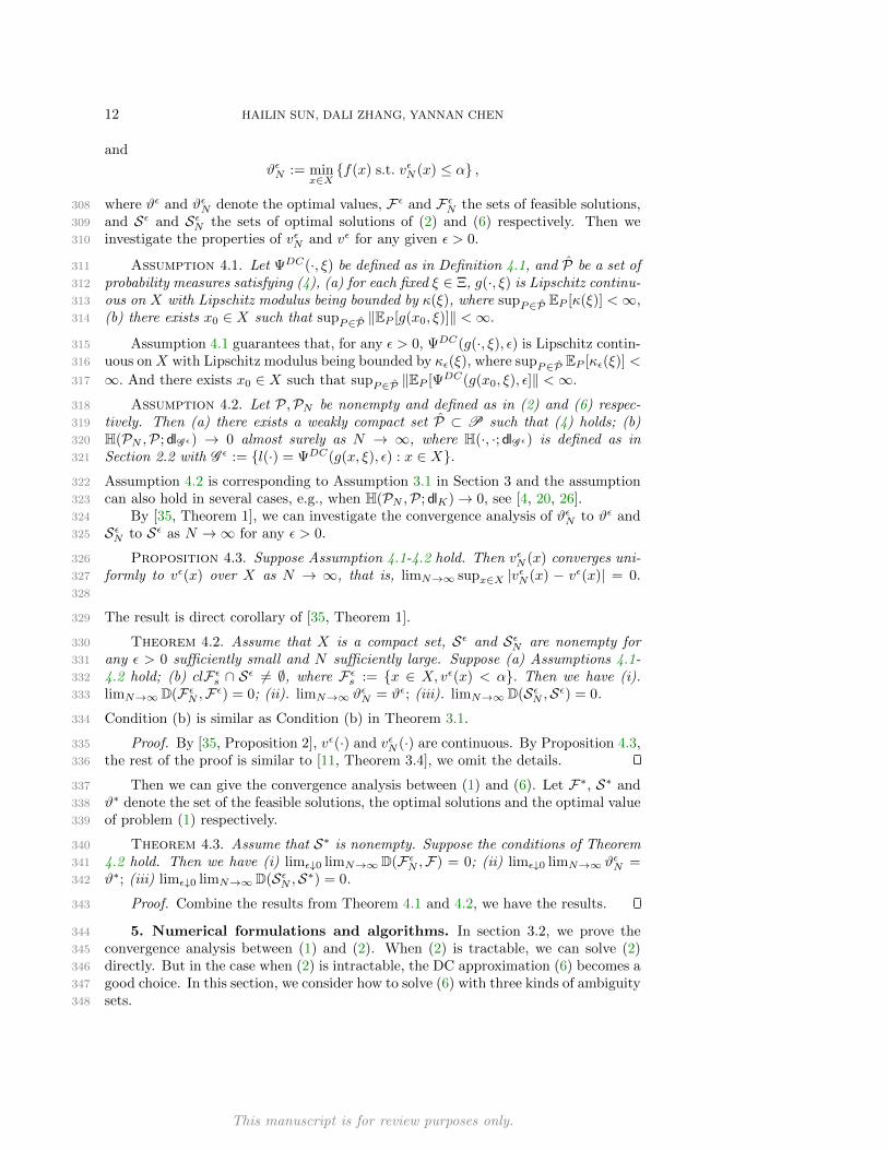
where ϑε and ϑεN denote the optimal values, Fε and FεN the sets of feasible solutions,308

and Sε and SεN the sets of optimal solutions of (2) and (6) respectively. Then we309

investigate the properties of vεN and vε for any given ε > 0.310

Assumption 4.1. Let ΨDC(·, ξ) be defined as in Definition 4.1, and P be a set of311

probability measures satisfying (4), (a) for each fixed ξ ∈ Ξ, g(·, ξ) is Lipschitz continu-312

ous on X with Lipschitz modulus being bounded by κ(ξ), where supP∈P EP [κ(ξ)] <∞,313

(b) there exists x0 ∈ X such that supP∈P ‖EP [g(x0, ξ)]‖ <∞.314

Assumption 4.1 guarantees that, for any ε > 0, ΨDC(g(·, ξ), ε) is Lipschitz contin-315

uous on X with Lipschitz modulus being bounded by κε(ξ), where supP∈P EP [κε(ξ)] <316

∞. And there exists x0 ∈ X such that supP∈P ‖EP [ΨDC(g(x0, ξ), ε]‖ <∞.317

Assumption 4.2. Let P,PN be nonempty and defined as in (2) and (6) respec-318

tively. Then (a) there exists a weakly compact set P ⊂ P such that (4) holds; (b)319

H(PN ,P; dlG ε) → 0 almost surely as N → ∞, where H(·, ·; dlG ε) is defined as in320

Section 2.2 with G ε := l(·) = ΨDC(g(x, ξ), ε) : x ∈ X.321

Assumption 4.2 is corresponding to Assumption 3.1 in Section 3 and the assumption322

can also hold in several cases, e.g., when H(PN ,P; dlK)→ 0, see [4, 20, 26].323

By [35, Theorem 1], we can investigate the convergence analysis of ϑεN to ϑε and324

SεN to Sε as N →∞ for any ε > 0.325

Proposition 4.3. Suppose Assumption 4.1-4.2 hold. Then vεN (x) converges uni-326

formly to vε(x) over X as N → ∞, that is, limN→∞ supx∈X |vεN (x) − vε(x)| = 0.327

328

The result is direct corollary of [35, Theorem 1].329

Theorem 4.2. Assume that X is a compact set, Sε and SεN are nonempty for330

any ε > 0 sufficiently small and N sufficiently large. Suppose (a) Assumptions 4.1-331

4.2 hold; (b) clFεs ∩ Sε 6= ∅, where Fεs := x ∈ X, vε(x) < α. Then we have (i).332

limN→∞ D(FεN ,Fε) = 0; (ii). limN→∞ ϑεN = ϑε; (iii). limN→∞D(SεN ,Sε) = 0.333

Condition (b) is similar as Condition (b) in Theorem 3.1.334

Proof. By [35, Proposition 2], vε(·) and vεN (·) are continuous. By Proposition 4.3,335

the rest of the proof is similar to [11, Theorem 3.4], we omit the details.336

Then we can give the convergence analysis between (1) and (6). Let F∗, S∗ and337

ϑ∗ denote the set of the feasible solutions, the optimal solutions and the optimal value338

of problem (1) respectively.339

Theorem 4.3. Assume that S∗ is nonempty. Suppose the conditions of Theorem340

4.2 hold. Then we have (i) limε↓0 limN→∞D(FεN ,F) = 0; (ii) limε↓0 limN→∞ ϑεN =341

ϑ∗; (iii) limε↓0 limN→∞D(SεN ,S∗) = 0.342

Proof. Combine the results from Theorem 4.1 and 4.2, we have the results.343

5. Numerical formulations and algorithms. In section 3.2, we prove the344

convergence analysis between (1) and (2). When (2) is tractable, we can solve (2)345

directly. But in the case when (2) is intractable, the DC approximation (6) becomes a346

good choice. In this section, we consider how to solve (6) with three kinds of ambiguity347

sets.348



5.1. MPDRCC with matrix moment constraints. Consider the MPDRCC349

(1) with matrix moment constraints350

(1) P :=

P ∈P(Ξ) :

EP [Φi(ξ)] = µi, for i = 1, · · · , pEP [Φi(ξ)] µi, for i = p+ 1, · · · , q,

,351

Ξ ⊂ IRk is compact, Φi can be vector valued and/or symmetric matrix valued functions352

and µi can be vectors and/or symmetric matrices. Then the DC approximation of353

the problem is problem (2) with ambiguity set P, and its data-driven approxiamtion354

problem is355

(2)

minx∈X

f(x)

s.t. supP∈PN

EP [ΨDC(g(x, ξ), ε)] ≤ α,356

where

PN :=

P ∈P(ΞN ) :

EP [Φi(ξ)] = µNi , for i = 1, · · · , pEP [Φi(ξ)] µNi , for i = p+ 1, · · · , q

,

ΞN := ξ1, · · · , ξN is a discrete subset of Ξ and

βN := maxξ∈Ξ

min1≤i≤N

‖ξ − ξi‖

such that βN → 0 as N → ∞. Note that by convergence analysis between CP andPN in [4], Assumption 4.2 holds. Assume the Slater type condition (STC for short)

(1, 0) ∈ int(EP [1],EP [Φ(ξ)]) + 0p+1 × K : P ∈M+,

holds, where K := Snp+1×np+1

+ × · · · × Snq×nq+ ; see [33, condition (3.12)] for generalmoment problems. Then the constraints of problem (2) can be reformulated as itsdual form:

min(λ0,Λ)∈Λ

supP∈P(ΞN )

EP

[ΨDC(g(x, ξ), ε)− λ0 −

q∑i=1

〈Λi,Φi(ξ)〉

]+ λ0 +

q∑i=1

〈µNi ,Λi〉 ≤ α

where Λ := (λ0,Λ) : λ0 ∈ IR, Λi ∈ Sni , i = 1, · · · , p, and Λi 0, for i = p +357

1, · · · , q. Consequently, problem (2) can be reformulated as358

(3)

min(x,λ0,Λ)∈X×Λ

f(x)

s.t. λ0 +

q∑i=1

〈µNi ,Λi〉 ≤ α,

ΨDC(g(x, ξ), ε)− λ0 −q∑i=1

〈Φi(ξ),Λi〉 ≤ 0, ∀ξ ∈ ΞN .

359

Note that if g(x, ξ) is a convex function, then

ΨDC(g(x, ξ), ε) =1

ε((g(x, ξ))+ − (g(x, ξ)− ε)+) = ΨDC

1 (g(x, ξ), ε)−ΨDC2 (g(x, ξ), ε)

is a DC function, where

ΨDC1 (g(x, ξ), ε) :=

1

ε(g(x, ξ))+ and ΨDC

2 (g(x, ξ), ε) :=1

ε(g(x, ξ)− ε)+

are convex functions. Moreover, (3) is a DC constrained minimization problem and360

can be solved by the penalty and augmented Lagrangian method proposed in [21], see361

Section 5.4 for details.362



5.2. MPDRCC with ball constraints based on wasserstein distance. In363

this subsection, we consider how to approximate MPDRCC (1) with ball constraints364

based on wasserstein distance: Bδ(P0) := P ∈P(Ξ) : D(P0, P ; dlK) ≤ δ.365

By the DC approximation method proposed in Section 4, the MPDRCC (1) with366

ball constraints based on wasserstein distance can be approximated by367

(4)

minx∈X

f(x)

s.t. supP∈Bδ(P0)

EP [ΨDC(g(x, ξ), ε)] ≤ α.368

Note that since P0 is the center distribution of the random variable and might be369

continuous distribution or unknown distribution, problem (4) is still not easy to solve.370

In the rest of this subsection, we consider a data-driven approximation to problem (4).371

We use an emprical distribution PN = 1N

∑Ni=1 δξi for ξi ∈ ΞN and |ΞN | = N372

(constructed by historical data, Monte Carlo method, Quasi Monte Carlo method,373

etc.) to approximate P0, and for any ε > 0 and ε > 0, we can find N0 such that for374

all N ≥ N0, ProbdlK(P0, PN ) ≤ ε ≥ 1− ε and ProbβN ≤ ε ≥ 1− ε (βN is defined375

in Section 5.1. Then the DC approximated data-driven MPDRCC is:376

(5)

minx∈X

f(x)

s.t. supP∈Bδ(PN )

EP [ΨDC(g(x, ξ), ε)] ≤ α,377

where Bδ(PN ) := P ∈ P(ΞN ) : dlK(PN , P ) ≤ δ and ΞN is the support set of378

PN . Note since that H(Bδ(P ),Bδ(PN ); dlK) → 0 as dlK(P, PN ) → 0 and βN → 0,379

Assumption 4.2 holds, see [4].380

By [8, Theorem 1], problem (5) equivalent to381

(6)

minx∈X,λ≥0

f(x)

s.t. λδ − 1

N

N∑i=1

(λd(ξi, ξi)−ΨDC(g(x, ξi), ε)) ≤ α, ∀ζ ∈ ΠNi=1ΞiN ,

382

where ΞiN = ΞN and ζ = (ξ1, · · · , ξN ).383

Note that (6) is also a DC constrained minimization problem and can be solved384

by the penalty and augmented Lagrangian method proposed in [21] (see Section 5.4).385

5.3. MPDRCC with ambiguity set constructed through KL-divergence.386

We also consider the MPDRCC (1) with ambiguity set constructed through KL-387

divergence. KL-divergence is introduced by Kullback and Leibler [19]. Let p0 and p388

denote the density functions of true probability measure P0 and its perturbation P389

respectively. Then KL-divergence can be used to measure the deviation of p from p0390

as DKL(P‖P0) =∫

Ξp(ξ) log

(p(ξ)p0(ξ)

)dξ, and the ambiguity set can be constructed as391

(7) PηKL(P0) := P ∈P : DKL(P‖P0) ≤ η.392

When P0 is a discrete distribution, we understand p0(ξ) is the probability mass func-393

tion and the integral as the summation.394

By [16, 18], let α := supt>0e−η(t+1)α−1

t , MPDRCC (1) with the ambiguity set (7)395

can be written as396

(8)minx∈X

f(x)

s.t. EP0[1g(x,ξ)>0(ξ)] ≤ α.

397



By the DC approximation method proposed in Section 4, the chance constraint of398

MPDRCC (8) can be approximated by EP0[ΨDC(g(x, ξ), ε)] ≤ α, and we can use399

sample average approximation (SAA) method to approximate the DC approximated400

(8) as follows:401

(9)minx∈X

f(x)

s.t. 1N

∑Ni=1 ΨDC(g(x, ξi), ε) ≤ α,

402

where ξiNi=1 are i.i.d. samples of ξ. Problem (9) is still a DC constrained problem403

and can be solved by the penalty and augmented Lagrangian method proposed by404

[21] (see Section 5.4). Note also that the convergence analysis of SAA problem (9)405

has been investigated in [36].406

5.4. Algorithm for DC constrained DC minimization. In [21], Lu et al.407

propose a penalty and augmented Lagrangian method for solving DC constrained DC408

minimization. We will apply their method to solve our problems. For the complement409

of the paper, we write their algorithm as follows.410

Consider DC constrained DC minimization411

(10)min φ0(x)− ψ0(x)s.t. φi(x)− ψi(x) ≤ 0, ∀i = 1, · · · , l,

x ∈ X,412

where X ⊆ IRn is a closed convex set, ψi(x) = maxj∈Ji ψi,j(x), Ji = 1, 2, · · · , Ji413

for i = 0, 1, · · · , l, φi, ψi,j are continuously differentiable and convex functions.414

Given ρ ≥ 1, define the penalty function:

Fρ(x) = φ0(x)− ψ0(x) + ρ

l∑i=1

[φi(x)− ψi(x)]+.

Moreover, given x ∈ X and ε ≥ 0, we define

J (x, ε) = (j0, j1, . . . , jl) | ji ∈ Ji, ψi,ji(x) ≥ ψi(x)− ε,∀i = 0, 1, . . . , l.

By choosing J = (j0, j1, · · · , jl) ∈ J (x, ε), we define

Qρ(x; x, J) = φ0(x)−ψ0,j0(x)−∇ψ0,j0(x)>(x−x)+ρ

l∑i=1

[φi(x)− ψi,ji(x)−∇ψi,ji(x)>(x− x)

]+.

Clearly, Qρ(x; x, J) is a convex function. The penalty method for solving (10) is415

presented in Algorithm 1.416

Remark 6. In practice, since Fρk(x) ≤ Qρk(x; x, J) for all x ∈ X and Qρk(x; x, J)417

is a convex function, we only need to solve minx∈X Qρk(x; x, J) for properly choosing418

x ∈ X and J ∈ J (xk, ε). See [21] for more details.419

6. Numerical Experiments. In this section, we show three numerical exam-420

ples. The first and second examples are used to verify the convergence results in421

Section 3 and 4. The third example is used to test effectiveness of numerical formu-422

lations and algorithm in Section 5. In the numerical tests, we only focus on the case423

when ambiguity sets are constructed by moment information.424



Algorithm 1 A penalty method for solving DC minimization (10).

1: Choose ε > 0, ρ0 ≥ 1, σ > 1, and a positive sequence ηk → 0 as k → ∞. Setk ← 0.

2: while not converged do3: Find an approximate solution xk of the penalty subproblem

minx∈X

Fρk(x)

such that xk ∈ X and Fρk(xk) ≤ Qρk(x;xk, J) + ηk,∀x ∈ X,∀J ∈ J (xk, ε).4: Set ρk+1 ← σρk and k ← k + 1.5: end while

Example 6.1 (Academic example 1). To verify Theorem 3.1, we design this ex-periment. Let ϑ and S be the optimal value and the optimal solution set of the program(1) respectively with ambiguity set

P = P ∈P(IR) : EP [ξ] = µ,EP [ξξT ] = Σ + µµT .

We consider a constraint function g(x, ξ) = y0(x) + y(x)>ξ. Moreover, let ϑN andSN be the optimal value and the optimal solution set of the data-driven approximationproblem (2) with

PN = P ∈P(IR) : EP [ξ] = µN ,EP [ξξT ] = ΣN + µNµTN.

According to [45], since g(x, ξ) = y0(x) + y(x)>ξ is linear in ξ, program (1) and (2)425

could be represented as tractable SDP formulas426

min f(x)

s.t. M 0, β +1

α〈Ω,M〉 ≤ 0,

M −[

0 12y(x)

12y(x)> y0(x)− β

] 0,

x ∈ X, β ∈ R, M ∈ Sn+1,

and

min f(x)

s.t. M 0, β +1

α〈ΩN ,M〉 ≤ 0,

M −[

0 12y(x)

12y(x)> y0(x)− β

] 0,

x ∈ X, β ∈ R, M ∈ Sn+1,

427

where Ω =

[Σ + µµ> µµ> 1

], and ΩN =

[ΣN + µNµ

>N µN

µ>N 1

], µ, µN ∈ Rn and428

Σ,ΣN ∈ Sn.429

Consider a portfolio optimization problem over n products. The portfolio x ∈ Rn+satisfies

∑i xi = 1. Our objective is the expectation of the difference of the total input

and the real outcome ξ>x: f(x) = 1− µ>x, where ξ ∼ N (µ,Σ) is the rate of return.Let g(x, ξ) = η − x>ξ. Then the chance constraint is

infP∈PN

P [η − x>ξ ≤ 0] ≥ 1− α.



In our experiment, we set n = 10, α = 0.05, η = 0.1, µ = (0.6, 0.7, . . . , 1.5)>, and430

Σ =

0.4 −0.01 0 0.01 0 −0.01 0.01 0.01 0 −0.01−0.01 0.4 −0.01 −0.01 0 0.01 −0.01 −0.01 0.01 −0.01

0 −0.01 0.4 −0.01 0.01 0 0 0.01 0 00.01 −0.01 −0.01 0.4 0.01 −0.01 0.01 −0.01 0 0.01

0 0 0.01 0.01 0.4 −0.01 0.01 0.01 0.01 0.01−0.01 0.01 0 −0.01 −0.01 0.4 0.01 0 −0.01 −0.01

0.01 −0.01 0 0.01 0.01 0.01 0.4 −0.01 0.01 00.01 −0.01 0.01 −0.01 0.01 0 −0.01 0.4 0.01 0

0 0.01 0 0 0.01 −0.01 0.01 0.01 0.4 −0.01−0.01 −0.01 0 0.01 0.01 −0.01 0 0 −0.01 0.4

.431

By experiments, the optimal value is ϑ∗ = −0.3243, which is illustrated as a green432

line in Figure 3. Associated optimal solution is marked by five-pointed stars in the433

right column of Figure 4.434

Fig. 3. Optimal value v.s. the sample size. Fig. 4. Optimal solution v.s. the sample size.

Whereafter, we sample random variables ξ enjoying distribution N (µ,Σ) with435

sample size N = 20, 50, 100, 200, 500, 1000, 2000, 5000, 10000, respectively. For each436

N , we perform 30 tests. In each test, by estimating mean µN and covariance ΣN437

from associated sample, we compute estimated optimal value ϑN and estimated optimal438

solution xN . By this means, for a fix sample size N , there are thirty optimal values,439

whose median is illustrated as a red short line in Figure 3. The top and button440

edges of the blue box are respectively the 25th and 75th percentiles of these estimated441

optimal values corresponding to a fixed N , and the whiskers extend to the most extreme442

estimated optimal values. Clearly, as the sample size N increases, we see that the blue443

box shrinks and converges to the green line. Hence, we claim that the optimal value444

ϑN of data driven problems tends to ϑ∗ as N →∞.445

For each N , we also count the mean of estimated optimal solutions and illustrated446

components of the mean as squares in Figure 4. For each component, we also draw447

a line connecting estimated solutions to the true one. By Figure 4, we see these448

lines tend to the horizontal direction smoothly as N increases. Therefore, the optimal449

solution set SN of the data driven problems converges to the true solution set S∗ as450

the sample size N tends to infinity.451

Example 6.2 (Academic example 2). Our second example is used to verify theconvergence analysis proposed in Section 4.2. We consider problem (1) with ambiguityset

P = P ∈P(Ξ) : EP [ξ] = µ,EP [ξξT ] = Σ + µµT .



By using the DC approximate scheme (1) with data-driven approximation, we con-struct data driven approximated DC approximation problem (6) with approximationparameter ε and the set of uncertain distributions characterized by statistics fromhistorical samples:

PN = P ∈P(ΞN ) : EP [ξ] = µ,EP [ξξT ] = Σ + µµT ,

where ΞN is a discrete approximation of Ξ with |ΞN | = N such that ΞN1⊂ ΞN2

⊂ Ξ452

for any 0 ≤ N1 ≤ N2 and βN → 0 as N →∞. By [4, Theorem 3.1], H(P,PN ; dlG ε)→453

0 as N →∞.454

In this example, we consider a portfolio x ∈ [0, 1] and a risk-free investment455

(1−x). Parameters are set as µ = 1.1, Σ = 0.05, Ξ = [−50, 50], κ = 2, y0(x) = 13 , and456

α = 0.1, y(x) = −x, i.e., g(x, ξ) = 13 − x

>ξ. We divide the support set Ξ = [−50, 50]457

into (N − 1) equal parts and hence have N end points of all small intervals. We solve458

problem (6) in this example by Algorithm 1 with different N and ε. Let ϑεN denote the459

optimal value of (6) in this example with corresponding ε and N , the numerical results460

are shown as in Table 1. For a given N and ε, the first number in the associated cell461

is the optimal value ϑεN of (6) in this example, and the vector in the second line of462

the cell is the optimal solution (xεN , 1− xεN ).463

Table 1Optimal values and optimal solutions

Solving (6) in this example ε = 0.01 ε = 0.001 ε = 0.0001

N = 201 −1.0250 −1.0250 −1.0250

(0.5000, 0.5000)> (0.5000, 0.5000)> (0.5000, 0.5000)>

N = 501 −1.0250 −1.0250 −1.0247

(0.5000, 0.5000)> (0.5000, 0.5000)> (0.5555, 0.4445)>

N = 1001 −1.0250 −1.0247 −1.0222

(0.5000, 0.5000)> (0.5543, 0.4457)> (0.6665, 0.3335)>

N = 2001 −1.0250 −1.0239 −1.0192

(0.5013, 0.4987)> (0.6045, 0.3955)> (0.7405, 0.2595)>

SDP upper bound: ϑ = −1.0173 (x, 1 − x)> = (0.7767, 0.2233)>

Let ϑΞ be the optimal value of (1) in this example. Note that since

ΨDC(g(x, ξ), ε1) ≤ ΨDC(g(x, ξ), ε2) ≤ 1g(x,ξ)>0(g(x, ξ))

for any x ∈ X, ε1 ≥ ε2 > 0 and ΞN1⊂ ΞN2

⊂ Ξ for any 0 ≤ N1 ≤ N2, then thefeasible set of problem (6) in this example shrinks with ε ↓ 0 and N → ∞, and wehave ϑε1N1

≤ ϑε2N2≤ ϑΞ. Moreover, let ϑ denote the optimal value of problem (1) with

ambiguity set

P = P ∈P(IR) : EP [ξ] = µ,EP [ξξT ] = Σ + µµT .

Note that in this case, P ⊂ P and problem (1) can be solved by the SDP reformulation464

in [45] effectively. Then we have ϑ ≥ ϑΞ ≥ ϑε2N2≥ ϑε1N1

. The optimal value ϑ and the465

associated optimal solution are addressed in the last line of Table 1 as the “SDP upper466

bound”. However, when ε sufficiently large and N sufficiently large, we can see from467

the table that ‖(ϑ−ϑεN )‖ decreases and becomes very small, note that ϑΞ is between ϑ468

and ϑεN , which shows the convergence result. Note also that when ε is not sufficiently469

large and N is not sufficiently large, the feasible set of problem (6) in this example470



may be too large such that (0.5, 0.5)T is included in it, then the constraint is inactive471

and the optimal solution and optimal value are located on (0.5, 0.5)T and −1.025, see472

Table 1 for details.473

Example 6.3. In the numerical tests, we consider a portfolio optimization prob-474

lem based on the data set (historical return rates) of the stocks in the NASDAQ-100475

index (between January 2013 and January 2017). There are 100 stocks with 1000476

historical return rates, i.e., n = 100 and the sample size N = 1000.477

The portfolio optimization problem is constructed over a set of stocks 1, 2, . . . ,478

n(≤ 100) where we index the stocks in the subset of NASDAQ-100 index by i =479

1, 2, . . . , n. The loss function to the investor is the gap between the anticipated return480

η0 = 1 and the real outcome r>(ξ)x where x is the normalized portfolio (i.e., x :=481

(x1, · · · , xn), xi ≥ 0 for i = 1, 2, . . . , n, and x1 + · · · + xn = 1) into the stocks.482

Hence we have that the objective function in (6) being f(x) = 1 − 1N

∑Nj=1 r(ξ

j)>x.483

Whereafter, we define g(x, ξ) by a nonlinear form g(x, ξ) := exp(µ(η1 − r(ξ)>x)

)−1,484

where g(x, ξ) is a nonlinear function of x. In the tests, we set µ = 0.1 and η1 = 0.9.485

Let ΞN := ξ1, · · · , ξN and rNi (ξj) be the return rates of stock i at historicaltrading day j for i = 1, . . . , n and j = 1, . . . , N . The uncertain distribution set isdefined as

PN =

P ∈P(ΞN ) :

EP [ri(ξ)] = µi,EP[(ri(ξ)− µi)2

]≤ γΣi,

∀i = 1, . . . , n

,

where γ = 1.1, µi = 11000

∑1000j=1 r

Ni (ξj) and Σi = 1

1000

∑1000j=1

(rNi (ξj)− µi

)2.486

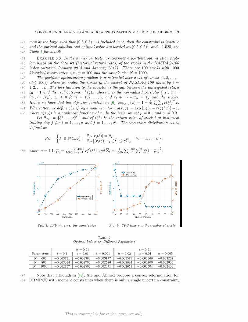
Fig. 5. CPU time v.s. the sample size Fig. 6. CPU time v.s. the number of stocks

Table 2Optimal Values vs. Different Parameters

α = 0.01 ε = 0.01Parameters ε = 0.1 ε = 0.01 ε = 0.001 α = 0.02 α = 0.01 α = 0.005

N = 600 −0.003731 −0.003368 −0.003177 −0.003579 −0.003368 −0.003262N = 800 −0.003034 −0.002700 −0.002526 −0.002894 −0.002700 −0.002603N = 1000 −0.002757 −0.002504 −0.002371 −0.002651 −0.002504 −0.002430

Note that although in [42], Xie and Ahmed propose a convex reformulation for487

DRMPCC with moment constraints when there is only a single uncertain constraint,488



they require the random function −g(x, ξ) is concave w.r.t. x and convex w.r.t. ξ, so489

their convex reformulation can not cover Example 6.3.490

We implement the DC approximation method and Algorithm 1 to solve the prob-491

lem. We perform the comparative analysis by varying parameter α, sample size N492

and the number of stocks. First we fix the number of stocks being 20, α = 0.02 and493

ε = 0.01, and increase the sample size N from 100 to 1000 and record the optimal494

value and the CPU time used for solving the problem. The result is given in Figure495

5. Note that with the increasing of N , the ambiguity set is enlarging, which leads to496

the increasing of the optimal values.497

Second we fix the sample size being N = 200, α = 0.02 and ε = 0.01 and increase498

the number of stocks from 10 to 100 and record the optimal value and the CPU time499

used for solving the problem. The result is given in Figure 6. Note that with the500

increasing of number of stocks, the investigator has more choices, and this leads to501

the decreasing of the optimal values.502

In the third set of test, we vary the parameters α from 0.02 to 0.005 and the DC503

approximate parameters in function ΨDC(•, ξ) from 0.1 to 0.001 to verify the optimal504

values solved from (6) in this example. All other parameters are fixed as previous505

experiments. Resulting optimal values are reported in Table 2. We can see from506

Table 2 that with ε ↓ 0 and α ↓ 0, the optimal values increase, which is consistent507

with the fact that the feasible set of (6) in this example shrinks with ε ↓ 0 and α ↓ 0.508

7. Conclusion. This paper investigates the convergence of optimal value and509

the optimal solutions of data-driven approximation of MPDRCC without assuming510

the continuity of distributional robust probability functions. One important issue511

to be handled is the lower semi-continuity of the distributionally robust probability512

functions, which is used to replace the continuity condition of distributionally robust513

probability functions.514

Moreover, for the case when the MPDRCC is intractable, we propose a data-515

driven approximated DC approximation method for MPDRCC with the corresponding516

convergence analysis. The approximated problem can be solved by recent advances517

of DC algorithms effectively. One main advantage of the DC approximation method518

is the consistency of the feasible sets when the DC parameter ε ↓ 0, which allows us519

to avoid the continuity condition of distributionally robust probability functions. The520

preliminary numerical tests verify the convergence analysis and show the effectiveness521

of the proposed approximation methods.522

REFERENCES523

[1] K. B. Athreya and S. N. Lahiri, Measure theory and probability theory, Springer Science &524Business Media, New York, 2006.525

[2] G. Calafiore and L. E. Ghaoui, Distributionally robust chance-constrained linear programs526with applications, Journal of Optimization Theory and Application, 130 (2006), pp. 1–22.527

[3] A. Charnes, W. Cooper, and G. H. Symonds, Cost horizons and certainty equivalents: an528approach to stochastic programming of heating oil, Management Science, 4 (1958), pp. 235–529263.530

[4] Y. Chen, H. Sun, and H. Xu, Decomposition methods for solving two-stage distributionally531robust optimization, Optimization-online, (2019).532

[5] Z. Chen, D. Kuhn, and W. Wiesemann, Data-driven chance constrained programs over wasser-533stein balls, 2018, https://arxiv.org/abs/1809.00210.534

[6] D. Dentcheva and G. Martinez, Regularization methods for optimization problems with prob-535abilistic constraints, Mathematical Programming, 138 (2013), pp. 223–251.536

[7] E. Erdogan and G. Iyengar, Ambiguous chance constrained problems and robust optimization,537Mathematical Programming, 107 (2006), pp. 37–61.538


https://arxiv.org/abs/1809.00210


[8] R. Gao and A. J. Kleywegt, Distributionally robust stochastic optimization with wasserstein539distance, 2016, https://arxiv.org/abs/1604.02199.540

[9] A. Geletu, A. Hoffmann, M. Kloppel, and P. Li, An inner-outer approximation approach to541chance constrained optimization, SIAM Journal on Optimization, 27 (2017), pp. 1834–1857.542

[10] A. L. Gibbs and F. E. Su, On choosing and bounding probability metrics, International statis-543tical review, 70 (2002), pp. 419–435.544

[11] S. Guo, H. Xu, and L. Zhang, Stability analysis for mathematical programs with distribution-545ally robust chance constraint, SIAM Journal on Optimization, 27 (2017), pp. 784–816.546

[12] G. A. Hanasusanto, V. Roitch, D. Kuhn, and W. Wiesemann, A distributionally robust per-547spective on uncertainty quanlification and chance constrained programming, Mathematical548Programming, 151 (2015), pp. 427–439.549

[13] G. A. Hanasusanto, V. Roitch, D. Kuhn, and W. Wiesemann, Ambiguous joint chance con-550straints under mean and dispersion information, Operations Research, 65 (2017), pp. 751–551767.552

[14] R. Henrion and C. Strugarek, Convexity of chance constraints with dependent random vari-553ables: The use of copulae, in Stochastic Optimization Methods in Finance and Energy:554New Financial Products and Energy Market Strategies, M. Bertocchi, G. Consigli, and M.555A. H. Dempster, eds., Springer, Now York, 2011.556

[15] L. J. Hong, Y. Yang, and L. Zhang, Sequential convex approximations to joint chance con-557strained programs: a monte carlo approach, Operations Research, 59 (2011), pp. 617–630.558

[16] Z. Hu and L. J. Hong, Kullback-leibler divergence constrained distributionally robust optimiza-559tion, 2013, http://www.optimization-online.org/DB FILE/2012/11/3677.pdf.560

[17] Z. Hu, L. J. Hong, and L. Zhang, A smooth monte carlo approach to joint chance-constrained561programs, IIE Transactions, 45 (2013), pp. 716–735.562

[18] R. Jiang and Y. Guan, Data-driven chance constrained stochastic program, Mathematical563Programming, 158 (2016), pp. 291–327.564

[19] S. Kullback and R. Leibler, On information and sufficiency, Annals of Mathematical Statis-565tics, 22 (1951), pp. 79–86.566

[20] Y. Liu, A. Pichler, and H. Xu, Discrete approximation and quantification in distributionally567robust optimization, Mathematics of Operations Research, 44 (2018), pp. 19–37.568

[21] Z. Lu, Z. Sun, and Z. Zhou, Penalty and augmented lagrangian methods for a class of struc-569tured nonsmooth dc constrained dc program, Manuscript, (2019).570

[22] J. Luedtke and S. Ahmed, A sample approximation approach for optimization with probabilis-571tic constraints, SIAM Journal on Optimization, 19 (2008), pp. 674–699.572

[23] L. B. Miller and H. Wagner, Chance-constrained programming with joint constraints, Oper-573ations Research, 13 (1965), pp. 930–945.574

[24] A. Nemirovski and A. Shapiro, Convex approximations of chance constrained programs, SIAM575Journal on Optimization, 17 (2006), pp. 969–996.576

[25] B. K. Pagnoncelli, S. Ahmed, and A. Shapiro, Sample average approximation method for577chance constrained programming: Theory and applications, Journal of Optimization Theory578and Applications, 142 (2009), pp. 399–416.579

[26] A. Pichler and H. Xu, Quantitative stability analysis for minimax distributionally robust580risk optimization, Mathematical Programming, (2018), https://link.springer.com/article/58110.1007/s10107-018-1347-4.582

[27] A. Prekopa, On probabilistic constrained programming. In: Proceedings of the Princeton Sym-583posium on Mathematical Programming, Princeton University Press, Princeton, 1970.584

[28] A. Prekopa, Probabilistic programming, in Stochastic Programming, A. Ruszczynski and A.585Shapiro, eds., Elsevier, Amsterdam, 2003.586

[29] S. T. Rachev, Probability Metrics and the Stability of Stochastic Models, John Wiley and Sons,587West Sussex, England, 1991.588

[30] W. Romisch, Stability of stochastic programming problems, in Stochastic Programming, A.589Ruszczynski and A. Shapiro, eds., Elsevier, Amsterdam, 2003.590

[31] R. Rockafellar and R. J.-B. Wets, Variational Analysis, Springer-Verlag, New York, 3th ed.,5912009.592

[32] F. Shan, X. T. Xiao, and L. W. Zhang, Convergence analysis on a smoothing approach to593joint chance constrained programs, Optimization, 65 (2016), pp. 2171–2193.594

[33] A. Shapiro, On duality theory of conic linear problems, in Semi-Infinite Programming: Recent595Advances, M. A. Goberna and M. A. Lopez, eds., Springer, New York, 2001.596

[34] A. Shapiro, D. Dentcheva, and A. Ruszczynski, Lectures on Stochastic Programming: Mod-597eling and Theory, SIAM, Philadelphia, 2009.598

[35] H. Sun and H. Xu, Convergence analysis for distributionally robust optimization and equilib-599rium problems, Mathematics of Operations Research, 41 (2016), pp. 377–401.600


https://arxiv.org/abs/1604.02199

http://www.optimization-online.org/DB_FILE/2012/11/3677.pdf

https://link.springer.com/article/10.1007/s10107-018-1347-4




[36] H. Sun, H. Xu, and Y. Wang, Asymptotic analysis of sample average approximation601forstochastic optimization problems with joint chance constraints via conditional value at602risk and difference of convex functions, Journal of Optimization Theory and Applications,603161 (2014), pp. 257–284.604

[37] W. van Ackooij, Chance Constrained Programming: With Applications in Energy Manage-605ment, , Ph.D. thesis,, Ecole Centrale, Paris, 2013.606

[38] W. van Ackooij, Eventual convexity of chance constrained feasible sets, Optimization, 64607(2015), pp. 1263–1284.608

[39] W. van Ackooij and R. Henrion, Gradient formulae for nonlinear probabilistic constraints609with gaussian and gaussian-like distributions, SIAM Journal on Optimization, 24 (2014),610pp. 1864–1889.611

[40] W. Xie, On distributionally robust chance constrained programs with wasserstein distance,612Optimization-online, (2018), https://arxiv.org/pdf/1806.07418.pdf.613

[41] W. Xie and S. Ahmed, Bicriteria approximation of chance constrained covering prob-614lems, Optimization-online, (2018), http://www.optimization-online.org/DB FILE/2018/61501/6411.pdf.616

[42] W. Xie and S. Ahmed, On deterministic reformulations of distributionally robust joint chance617constrained optimization problems, Mathematical Programminng, 28 (2018), pp. 1151–1182.618

[43] W. Yang and H. Xu, Distributionally robust chance constraints for non-linear uncertainties,619Mathematical Programminng, 155 (2016), pp. 231–265.620

[44] V. M. Zolotarev, Probability metrics, Teoriya Veroyatnostei i ee Primeneniya, 28 (1983),621pp. 264–287.622

[45] S. Zymler, D. Kuhn, and B. Rustem, Distributionally robust joint chance constraints with623second-order moment information, Mathematical Programming, 137 (2013), pp. 167–198.624


https://arxiv.org/pdf/1806.07418.pdf




convergence analysis and a dc approximation method … · 2019-11-07 · 1 convergence analysis and...

Documents