Categories in ControlJohn Baez and Jason Eberle

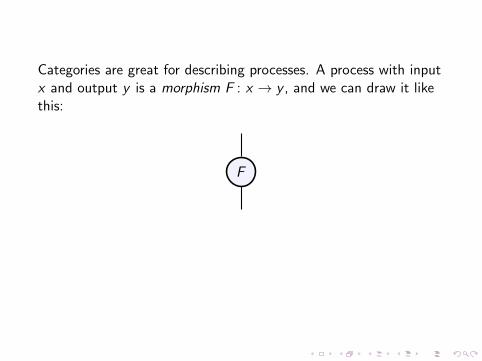
Categories are great for describing processes. A process with inputx and output y is a morphism F : x → y , and we can draw it likethis:

F

We can do one process after another if the output of the firstequals the input of the second:

F

G

Here we are composing morphisms F : x → y and G : y → z to geta morphism GF : x → z .

In a monoidal category, we can also do processes ‘in parallel’:

F G

Here we are ‘tensoring’ F : x → y and G : x ′ → y ′ to get amorphism F ⊗ G : x ⊗ x ′ → y ⊗ y ′.

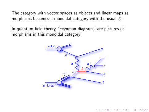
The category with vector spaces as objects and linear maps asmorphisms becomes a monoidal category with the usual ⊗.

In quantum field theory, ‘Feynman diagrams’ are pictures ofmorphisms in this monoidal category:

But why should quantum field theorists have all the fun? This isthe century of biology, and ecology.

Now is our chance to understand the biosphere, and stopdestroying it! We should be using category theory — andeverything else — to do these things.

Biologists use diagrams to describe the complex processes they findin life. They use at least three different diagram languages, asformalized in Systems Biology Graphical Notation.

We should try to understand these diagrams using all the tools ofmodern mathematics!

But let’s start with something easier: engineering. Engineers use‘signal-flow graphs’ to describe processes where signals flowthrough a system and interact:

Think of a signal as a smooth real-valued function of time:

f : R→ R

We can multiply a signal by a constant and get a new signal:

f

c

cf

We can integrate a signal:

f

∫∫f

Here is what happens when you push on a mass m with atime-dependent force F :

q

∫ v

∫ a

1m

F

Integration introduces an ambiguity: the constant of integration.But electrical engineers often use Laplace transforms to writesignals as linear combinations of exponentials

f (t) = e−st for some s > 0

Then they define

(∫f )(t) =

e−st

s

This lets us think of integration as a special case of scalarmultiplication! We extend our field of scalars from R to R(s), thefield of rational real functions in one variable s.

Let us be general and work with an arbitrary field k . For us, asignal-flow graph with m input edges and n output edges will standfor a linear map

F : km → kn

In other words: signal-flow graphs are pictures of morphisms inFinVectk , the category of finite-dimensional vector spaces over k ...where we make this into a monoidal category using ⊕, not ⊗.

We build these pictures from a few simple pieces.

First, we have scalar multiplication:

This is a notation for the linear map

k → kf 7→ cf

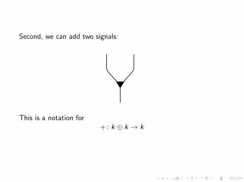
Second, we can add two signals:

This is a notation for+: k ⊕ k → k

Third, we can ‘duplicate’ a signal:

This is a notation for the diagonal map

∆: k → k ⊕ kf 7→ (f , f )

Fourth, we can ‘delete’ a signal:

This is a notation for the linear map

k → {0}f 7→ 0

Fifth, we have the zero signal:

This is a notation for the linear map

{0} → k0 7→ 0

Furthermore, (FinVectk , ⊕) is a symmetric monoidal category.This means we have a ‘braiding’: a way to switch two signals:

f

g f

g

This is a notation for the linear map

k ⊕ k → k ⊕ k(f , g) 7→ (g , f )

In a symmetric monoidal category, the braiding must obey a fewaxioms. I won’t list them here, since they are easy to find.

From these ‘generators’:

c

together with the braiding, we can build complicated signal flowdiagrams. In fact, we can describe any linear map F : km → km

this way!

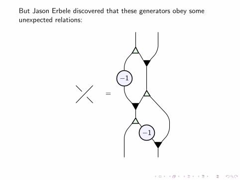
But Jason Erbele discovered that these generators obey someunexpected relations:

=

−1

−1

Luckily, they all follow from some comprehensible relations!

Theorem (Jason Eberle)

FinVectk is equivalent to the symmetric monoidal categorygenerated by the object k and these morphisms:

c

where c ∈ k , with the following relations.

Addition and zero make k into a commutative monoid:

==

=

Duplication and deletion make k into a cocommutative comonoid:

==

=

The monoid and comonoid operations are compatible, as in abialgebra:

=

= =

=

The ring structure of k can be recovered from the generators:

bc =b

cb + c = b c

1 =0 =

Scalar multiplication is linear (compatible with addition and zero):

c c=

c

c =

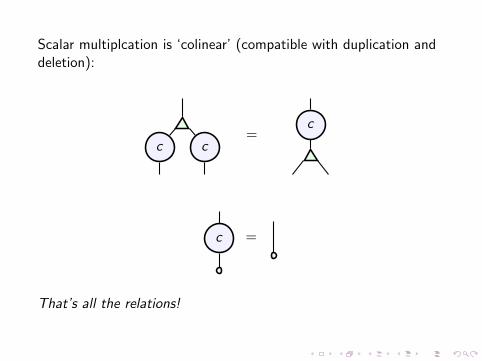
Scalar multiplcation is ‘colinear’ (compatible with duplication anddeletion):

c c=

c

c =

That’s all the relations!

However, control theory also needs more general signal-flowgraphs, which have ‘feedback loops’:

This is the most important concept in control theory: letting theoutput of a system affect its input.

To allow feedback loops we need morphisms more general thanlinear maps. We need linear relations!

A linear relation F : U V from a vector space U to a vectorspace V is a linear subspace F ⊆ U ⊕ V .

We can compose linear relations F : U V and G : V W andget a linear relation G ◦ F : U W :

G ◦ F = {(u,w) : ∃v ∈ V (u, v) ∈ F and (v ,w) ∈ G}.

A linear map φ : U → V gives a linear relation F : U V , namelythe graph of that map:

F = {(u, φ(u)) : u ∈ U}

Composing linear maps becomes a special case of composing linearrelations.

There is a symmetric monoidal category FinRelk with finite-dimensional vector spaces over the field k as objects and linearrelations as morphisms. This has FinVectk as a subcategory.

Fully general signal-flow diagrams are pictures of morphisms inFinRelk , typically with k = R(s).

Jason Erbele showed that besides the previous generators ofFinVectk , we only need two more morphisms to generate all themorphisms in FinRelk : the ‘cup’ and ‘cap’.

f = g

f g

f = g

f g

These linear relations say that when a signal goes around a bend ina wire, the signal coming out equals the signal going in!

More formally, the cup is the linear relation

∪ : k ⊕ k {0}

that is, a subspace∪ ⊆ k ⊕ k ⊕ {0}

given by:∪ = {(f , f , 0) : f ∈ k}

Similarly, the cap∩ : {0} k ⊕ k

is the subspace∩ ⊆ {0} ⊕ k ⊕ k

given by:∩ = {(0, f , f ) : f ∈ k}

Theorem (Jason Eberle)

FinRelk is equivalent to the symmetric monoidal categorygenerated by the object k and these morphisms:

c

where c ∈ k , and an explicit list of relations.

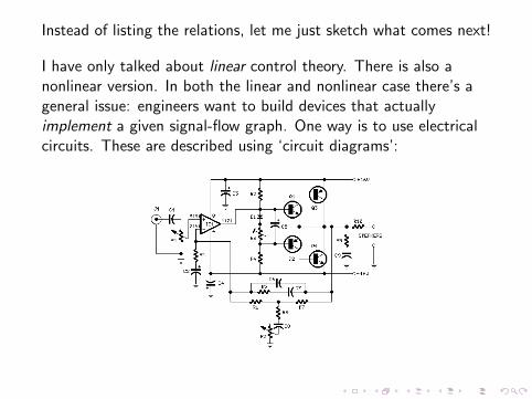
Instead of listing the relations, let me just sketch what comes next!

I have only talked about linear control theory. There is also anonlinear version. In both the linear and nonlinear case there’s ageneral issue: engineers want to build devices that actuallyimplement a given signal-flow graph. One way is to use electricalcircuits. These are described using ‘circuit diagrams’:

At least in the linear case, there is a category Circ whosemorphisms are circuit diagrams. Thanks to work in progress byBrendan Fong, we know there is a functor from this category toFinRelk :

Z: Circ → FinRelk

This functor says, for any linear circuit, how the voltages andcurrents on the input wires are related to those on the ouput wires.

However, we do not get arbitrary linear relations this way. Thespace of voltages and current on n wires,

kn ⊕ kn

is naturally a symplectic vector space. And the kind of linearrelation

F : km ⊕ km kn ⊕ kn

we get from a linear circuit is naturally a Lagrangian relation. Thatis,

F ⊆ (km ⊕ km)⊕ (kn ⊕ kn)

is a Lagrangian subspace: a maximal subspace on which thesymplectic 2-form vanishes! These are important in classicalmechanics.

So, we can see the beginnings of an interesting relation between:

control theory

electrical engineering

category theory

symplectic geometry

This should become even more interesting when we study nonlinearsystems. And as we move from the networks important inhuman-engineered systems to those important in biology andecology, the mathematics should become even more rich!

For more, see what the Azimuth Project is doing on networktheory:

www.azimuthproject.org